numerical modeling of crack formation in powder compaction
TRANSCRIPT

NUMERICAL MODELING OF
CRACK FORMATION
IN POWDER COMPACTION PROCESSES
Joaquın A. Hernandez Ortega
Xavier Oliver Olivella
Juan Carlos Cante Teran


Abstract
Powder metallurgy (P/M) is an important technique of manufacturing metal partsfrom metal in powdered form. Traditionally, P/M processes and products havebeen designed and developed on the basis of practical rules and trial-and-errorexperience. However, this trend is progressively changing. In recent years, thegrowing efficiencies of computers, together with the recognition of numerical sim-ulation techniques, and more specifically, the finite element method , as powerfulalternatives to these costly trial-and-error procedures, have fueled the interest ofthe P/M industry in this modeling technology. Research efforts have been devotedmainly to the analysis of the pressing stage and, as a result, considerable progresshas been made in the field of density predictions. However, the numerical simula-tion of the ejection stage, and in particular, the study of the formation of crackscaused by elastic expansion and/or interaction with the tool set during this phase,has received less attention, notwithstanding its extreme relevance in the quality ofthe final product.
The primary objective of this work is precisely to fill this gap by developing aconstitutive model that attempts to describe the mechanical behavior of the powderduring both pressing and ejection phases, with special emphasis on the representa-tion of the cracking phenomenon. The constitutive relationships are derived withinthe general framework of rate-independent, isotropic, finite strain elastoplasticity.The yield function is defined in stress space by three surfaces intersecting non-smoothly, namely, an elliptical cap and two classical Von Mises and Drucker-Prageryield surfaces. The distinct irreversible processes occurring at the microscopic levelare macroscopically described in terms of two internal variables: an internal hard-ening variable, associated with accumulated compressive (plastic) strains, and aninternal softening variable, linked with accumulated (plastic) shear strains. Theinnovative part of our modeling approach is connected mainly with the character-ization of the latter phenomenological aspect: strain softening. Incorporation of asoftening law permits the representation of macroscopic cracks as high gradientsof inelastic strains (strain localization). Motivated by both numerical and physicalreasons, a parabolic plastic potential function is introduced to describe the plasticflow on the linear Drucker-Prager failure surface. A thermodynamically consistentcalibration procedure is employed to relate material parameters involved in thesoftening law to fracture energy values obtained experimentally on Distaloy AEspecimens.
The discussion of the algorithmic implementation of the model is confined ex-
clusively to the time integration of the constitutive equations. Motivated by com-putational robustness considerations, a non-conventional integration scheme thatcombines advantageous features of both implicit and explicit method is employed.The basic ideas and assumptions underlying this method are presented, and thestress update and the closed-form expression of the algorithmic tangent modulistemming from this method are derived. This integration scheme involves, in turn,the solution at each time increment of the system of equations stemming from aclassical, implicit backward-Euler difference scheme. An iterative procedure basedon the decoupling of the evolution equations for the plastic strains and the internalvariables is proposed for solving these return-mapping equations. It is proved thatthis apparently novel method converges unconditionally to the solution regardlessof the value of the material properties.
To validate the proposed model, a comparison between experimental resultsof diametral compression tests and finite element predictions is carried out. Thevalidation is completed with the study of the formation of cracks due to elastic ex-pansion during ejection of an overdensified thin cylindrical part. Both simulationsdemonstrate the ability of the model to detect evidence of macroscopic cracks, clar-ify and provide reasons for the formation of such cracks, and evaluate qualitativelythe influence of variations in the input variables on their propagation. Besides, inorder to explore the possibilities of the numerical model as a tool for assisting in thedesign and analysis of P/M uniaxial die compaction (including ejection) processes,a detailed case study of the compaction of an axially symmetric multilevel part inan advanced CNC press machine is performed. Special importance is given in thisstudy to the accurate modeling of the geometry of the tool set and the externalactions acting on it (punch platen motions). Finally, the potential areas for futureresearch are identified.


ii

Table of Contents
1 Introduction 11.1 Motivation . . . . . . . . . . . . . . . . . . . . . . . . . . . . . . . . 11.2 Objective and scope . . . . . . . . . . . . . . . . . . . . . . . . . . . 21.3 Modeling viewpoint . . . . . . . . . . . . . . . . . . . . . . . . . . . . 3
1.3.1 Powder sub-system . . . . . . . . . . . . . . . . . . . . . . . . 31.3.2 Tooling sub-system . . . . . . . . . . . . . . . . . . . . . . . . 71.3.3 Interaction powder-tooling . . . . . . . . . . . . . . . . . . . . 9
1.4 Outline . . . . . . . . . . . . . . . . . . . . . . . . . . . . . . . . . . 9
2 Continuum modeling of the powder behavior 112.1 Phenomenological aspects within a one dimensional setting . . . . . 12
2.1.1 Densification phenomenon . . . . . . . . . . . . . . . . . . . . 122.1.2 Cracking phenomena and their modelling . . . . . . . . . . . 13
2.2 Kinematics of plastic large deformations . . . . . . . . . . . . . . . . 192.2.1 Multiplicative decomposition . . . . . . . . . . . . . . . . . . 21
2.3 Thermodynamic consistency . . . . . . . . . . . . . . . . . . . . . . . 232.3.1 Physical interpretation of changes in the value of the internal
energy . . . . . . . . . . . . . . . . . . . . . . . . . . . . . . . 242.3.2 Decomposition of the free energy function . . . . . . . . . . . 26
2.4 Elastic response . . . . . . . . . . . . . . . . . . . . . . . . . . . . . . 272.5 Plastic response . . . . . . . . . . . . . . . . . . . . . . . . . . . . . . 28
2.5.1 Internal variables . . . . . . . . . . . . . . . . . . . . . . . . . 292.5.2 Yield function . . . . . . . . . . . . . . . . . . . . . . . . . . 322.5.3 Flow rule . . . . . . . . . . . . . . . . . . . . . . . . . . . . . 342.5.4 Hardening laws . . . . . . . . . . . . . . . . . . . . . . . . . . 402.5.5 Softening laws . . . . . . . . . . . . . . . . . . . . . . . . . . 50
3 Integration of the constitutive equation 633.1 Preliminaries . . . . . . . . . . . . . . . . . . . . . . . . . . . . . . . 63
3.1.1 Implicit Backward-Euler and IMPLEX integrationschemes . . . . . . . . . . . . . . . . . . . . . . . . . . . . . . 66
3.2 Implicit integration scheme . . . . . . . . . . . . . . . . . . . . . . . 683.2.1 Modification of the evolution equations . . . . . . . . . . . . 723.2.2 Return mapping algorithm using a fractional-step based method. 78
iii

iv Table of Contents
3.3 IMPLEX integration scheme . . . . . . . . . . . . . . . . . . . . . . . 973.3.1 Algorithmic elastoplastic tangent moduli . . . . . . . . . . . . 101
4 Numerical assessment 1094.1 Introduction . . . . . . . . . . . . . . . . . . . . . . . . . . . . . . . . 109
4.1.1 Overview of the modeling setting . . . . . . . . . . . . . . . . 1104.2 Diametral compression test . . . . . . . . . . . . . . . . . . . . . . . 113
4.2.1 Results . . . . . . . . . . . . . . . . . . . . . . . . . . . . . . 1154.2.2 Discussion and concussions . . . . . . . . . . . . . . . . . . . 122
4.3 Pressing and ejection of a thin cylindrical part . . . . . . . . . . . . 1254.3.1 Results and discussion . . . . . . . . . . . . . . . . . . . . . . 1264.3.2 Conclusions . . . . . . . . . . . . . . . . . . . . . . . . . . . . 142
5 Modeling guidelines for industrial applications: compaction of amultilevel part 1455.1 Modeling of the compacting tool set . . . . . . . . . . . . . . . . . . 1475.2 External actions . . . . . . . . . . . . . . . . . . . . . . . . . . . . . 148
5.2.1 Theoretical and true prescribed conditions . . . . . . . . . . . 1525.3 Simulation of the pressing stage . . . . . . . . . . . . . . . . . . . . . 154
5.3.1 Estimation of the starting conditions . . . . . . . . . . . . . . 1545.3.2 Assessment of the effect of an innacurate description of tool-
ing motions . . . . . . . . . . . . . . . . . . . . . . . . . . . . 1585.3.3 Optimization of the pressing sequence . . . . . . . . . . . . . 165
5.4 Ejection . . . . . . . . . . . . . . . . . . . . . . . . . . . . . . . . . . 1735.4.1 Revised design . . . . . . . . . . . . . . . . . . . . . . . . . . 186
5.5 Conclusions . . . . . . . . . . . . . . . . . . . . . . . . . . . . . . . . 189
6 Concluding remarks 1936.1 On the general features of the proposed constitutive model . . . . . 193
6.1.1 The fracture modeling . . . . . . . . . . . . . . . . . . . . . . 1946.1.2 The thermodynamic framework . . . . . . . . . . . . . . . . . 194
6.2 On the integration of the constitutive equation . . . . . . . . . . . . 1956.3 On the robustness of the solution algorithm . . . . . . . . . . . . . . 1966.4 On the simulation technology . . . . . . . . . . . . . . . . . . . . . . 196
A Mathematical aspects of the continuum formulation 197A.1 Large strain kinematics . . . . . . . . . . . . . . . . . . . . . . . . . 197
A.1.1 Structure of the free energy function . . . . . . . . . . . . . . 203A.1.2 Lie derivative of some spatial tensors . . . . . . . . . . . . . . 207
A.2 Governing equation in generalized stresses . . . . . . . . . . . . . . . 212A.3 Continuum elastoplastic tangent moduli . . . . . . . . . . . . . . . . 216A.4 Derivation of the IMPLEX algorithmic elastoplastic tangent moduli 217

Table of Contents v
B Analytical study of the compaction of a cylindrical specimen 221B.1 Pressing stage . . . . . . . . . . . . . . . . . . . . . . . . . . . . . . . 221B.2 Assessment of the smallness of elastic strains . . . . . . . . . . . . . 225B.3 Release of axial pressure . . . . . . . . . . . . . . . . . . . . . . . . . 227
C Thermodynamic aspects 233C.1 Fulfilment of the Clausius-Duhem inequality . . . . . . . . . . . . . . 233
References 238

vi Table of Contents

List of Figures
2.1 Two step compaction procedure. (a) Pressure distribution (b) Den-sity distribution f(c) Compressibility curve . . . . . . . . . . . . . . . 13
2.2 Tensile test. Pre-peak distribution of: (a) strain (b) displacement. . 15
2.3 Stress-strain response. . . . . . . . . . . . . . . . . . . . . . . . . . . 16
2.4 Tensile test. Post-peak distribution of: (a) strain (b) displacement. . 16
2.5 Force-displacement response. . . . . . . . . . . . . . . . . . . . . . . 18
2.6 Fracture modes. In the opening mode or mode I the loads inducingfracture are perpendicular to the plane of the crack, as in the tensiletest we are describing. Modes II and III are shearing modes, withloads acting on the crack plane. . . . . . . . . . . . . . . . . . . . . . 19
2.7 Yield surfaces for two different states. (a) Drucker-Prager + ellipticalcap, for moderate level of compaction (b) Drucker-Prager + ellipticalcap + Von Mises, for high level of compaction (close to full density) 33
2.8 Direction of the plastic flow. (a) Associated flow (ellipse) + linearplastic potential function (b) Singularity at the vertex. . . . . . . . . 36
2.9 Parabolic plastic potential surface, for γ close to zero. . . . . . . . . 39
2.10 Hydrostatic yield stress in compression scy1h versus internal hardeningvariable ξh. Stress data represented in Cauchy (true) stress space.Experimental data from isostatic compression tests carried out byPavier [83] on Distaloy AE powder specimens. . . . . . . . . . . . . . 42
2.11 Radial to axial stress ratio versus internal hardening variable ξh.Experimental data obtained from simulated closed die compactionsconducted by Sinka et al. [94] on Distaloy AE powder specimens. . 43
2.12 Values of the elliptical cap yield surface eccentricity (s2h), obtainedby substituting the fitting equation (2.5.55) for ktr in Eq.(2.5.54),versus the internal hardening variable ξh. . . . . . . . . . . . . . . . 44
2.13 Cohesion, in Cauchy (true) stress space, against internal hardeningvariables ξh. Experimental data obtained by experiments carried outby Coube [25] on Distaloy AE powder specimens. . . . . . . . . . . . 45
vii

viii List of Figures
2.14 (a) Parameter of internal friction αh versus internal hardening vari-able ξh. Experimental data obtained by experiments carried out byCoube [25] on Distaloy AE powder specimens. (b) Representationof the stress path corresponding to a uniaxial compression test. Theparameter of internal friction αh cannot exceed the slope of suchstress path. . . . . . . . . . . . . . . . . . . . . . . . . . . . . . . . . 46
2.15 Experimental data from consolidated and over-consolidated com-pression tests (Pavier [83]) on Distaloy AE powder specimens. Iso-density contours employing (a) Drucker-Prager + Elliptical cap, (b)Drucker-Prager + Elliptical cap + Von-Mises . . . . . . . . . . . . . 47
2.16 (a) Definition of qcyint as the deviatoric stress measure at the inter-section of the Drucker-Prager and the elliptical cap (∂Ed,eτ . (b) VonMises parameter cvh vs internal hardening variable ξh. The curveAC corresponds to qcyint = qcyint(ξ
h), whereas BD is the quadratic fitto the data points obtained from the isodensity contours shown in2.15.b. . . . . . . . . . . . . . . . . . . . . . . . . . . . . . . . . . . 48
2.17 Young’s Modulus Ee vs internal hardening variable ξh. Experimen-tal data obtained by tests conducted by Pavier [83] on Distaloy AEpowder specimens. . . . . . . . . . . . . . . . . . . . . . . . . . . . . 49
2.18 (a) Tensile region in the p-q plane. Path OT represents the (elastic)stress trajectory in a uniaxial tensile test (b) Decrease of cohesiondue to the accumulation of plastic shear strain . . . . . . . . . . . . 52
2.19 Softening counterpart of the cohesion variable cs vs internal softeningvariable ξs. The continuum softening modulus H is the tangentialslope of this curve. The softening parameter H0 is the tangentialslope for ξs = ξs0. . . . . . . . . . . . . . . . . . . . . . . . . . . . . 54
2.20 Diametral compresison test. (a) The powder cylindrical specimenis subjected to two diametrically opposite forces. A crack developsalong the loaded diameter. (b) The specimen is split into two halvesalong the loaded diameter. . . . . . . . . . . . . . . . . . . . . . . . . 57
2.21 (a) Typical force versus displacement graph for a diametral com-pression test. (b) Area of the specimen employed to compute thefracture energy. . . . . . . . . . . . . . . . . . . . . . . . . . . . . . . 57
2.22 Fracture Energy vs ξh. Fracture Energy is defined herein per unitcurrent surface. Experimental values provided by Jonsen [50] (Dis-taloy AE powder specimens). . . . . . . . . . . . . . . . . . . . . . . 58
2.23 Intrinsic softening parameter H0 vs internal hardening variable ξh. . 61
3.1 Geometrical interpretation of the effect of coupling between elasticand plastic response. . . . . . . . . . . . . . . . . . . . . . . . . . . . 72
3.2 Function |1− es1/κe | vs η for a typical Distaloy AE powder. . . . . . 753.3 Different scenarios for the evolution of the internal hardening vari-
able. Only in situation labelled as A, the internal hardening evolves,i.e. ξhn+1 > ξhn. . . . . . . . . . . . . . . . . . . . . . . . . . . . . . . . 77
3.4 FSM scheme when only the elliptical yield surface is active. (a) Nodensification occurs . (b) Densification takes place. . . . . . . . . . 82

List of Figures ix
3.5 (a) Case in which the Drucker-Prager and elliptical yield surfacesare active in the first iteration of the FSM scheme. (b) Radicandof expression (3.2.66) versus the internal hardening variable. Thisgraph has been obtained using the calibrated curves for the DistaloyAE presented in the previous chapter. The positiveness of thesevalues ensures that the intersection ∂Ed,eτ exists for all ξh. . . . . . . 85
3.6 (a) Case in which the Drucker-Prager and elliptical yield surfacesare active in the second iteration. (b) Case in which only the ellipti-cal yield surface is active after performing the predictor step of thesecond iteration. . . . . . . . . . . . . . . . . . . . . . . . . . . . . . 87
3.7 Linearly convergent FSM sequence. . . . . . . . . . . . . . . . . . . . 933.8 Quadratically convergent FSM sequence. . . . . . . . . . . . . . . . . 95
4.1 Diametral compression test . . . . . . . . . . . . . . . . . . . . . . . 1144.2 Mesh layout . . . . . . . . . . . . . . . . . . . . . . . . . . . . . . . . 1164.3 Applied load versus deflection. Results for several number of time
steps. . . . . . . . . . . . . . . . . . . . . . . . . . . . . . . . . . . . 1164.4 Applied load against deflection. Result for several meshes, charac-
terized by the size h of their elements. . . . . . . . . . . . . . . . . . 1174.5 Applied load against deflection. Comparison between results com-
puted using a standard displacement-based formulation and a mixeddisplacement-pressure formulation. . . . . . . . . . . . . . . . . . . . 118
4.6 Applied load versus deflection. Comparison of computed results us-ing different elastic properties with experimental data collected byJonsen et al. [49]. The post-peak descending branch B-C is shownin magnified form. . . . . . . . . . . . . . . . . . . . . . . . . . . . . 118
4.7 (a) Images recorded experimentally by Jonsen et al [50]: initiationof the crack, point of maximum load, and end of the loading pro-cess. (b) Contour plots of computed cohesion corresponding to suchstages. (c) Contour plot of computed cohesion at the end of theloading process, showing the spatial grid used in the computation. . 120
4.8 Horizontal displacement contour lines. The graph shows the hori-zontal displacement measured along the horizontal diameter AAA´. 121
4.9 Dimensions of punches and initial die cavity. . . . . . . . . . . . . . . 1254.10 Initial mesh layout. . . . . . . . . . . . . . . . . . . . . . . . . . . . . 1264.11 Average axial pressure during pressing versus time. Results for sev-
eral number of time steps (uniformly spaced). The final portion ofthe curves is shown in magnified form. . . . . . . . . . . . . . . . . . 127
4.12 Average axial pressure during pressing versus time. Results for sev-eral number of time steps (constant and variable time steps). Thefinal portion of the curves is shown in magnified form. . . . . . . . . 128
4.13 (a) Number of iterations (global scheme) against time step numberand (b) length of the time interval versus time step number. Bothresults correspond to the case N = 50 (variable) steps shown in figure4.12 . . . . . . . . . . . . . . . . . . . . . . . . . . . . . . . . . . . . 129

x List of Figures
4.14 Average axial and radial pressure versus time (during pressing andaxial load release stages). Comparison between results computedby using two different contact algorithms, namely, a contact penaltystrategy, for two different penalty parameters Kp (which are propor-tional to Young’s modulus Ee of the compacting powder), and anaugmented lagrangian technique. . . . . . . . . . . . . . . . . . . . . 130
4.15 Axial stress, at a node located on the top surface of the compact,versus time (pressing and axial load release stages). Comparisonof the performance of penalty and augmented lagrangian contacttechniques. . . . . . . . . . . . . . . . . . . . . . . . . . . . . . . . . 131
4.16 (a) Contour plots of computed cohesion during emergence of thecompact from the die. The central and rightmost plots are displayedin magnified form in (b) and (c), respectively. (d) Qualitative de-scription of cracks observed in thin parts reported in the databaseof common cracks collected by Zenger et al. [112] . . . . . . . . . . . 134
4.17 (a) Eccentricity of the the resultant of lateral stresses causes bendingof the part. (b) Deflected shape showing the finite element mesh inthe simulated part (displacements scaled up 10 times). . . . . . . . . 135
4.18 Dieless case (a) Overly refined mesh (b) Contour plot of cohesionwith displacements scaled up 10 times. . . . . . . . . . . . . . . . . . 136
4.19 Stress trajectory in the mean-deviatoric stress plane of a point lo-cated on the top face of the part. (a) Pressing (path AB), release ofaxial load (path BCD) and ejection (up to the onset of bending, pathDE). (b) Enlarged view of the first quadrant. Path EF representselastic loading due to tensile bending stresses. Path FG indicatesdecrease of cohesion (green strength) due to strain softening. . . . . 137
4.20 Stress trajectory in the mean-deviatoric stress plane. Pressing andaxial pressure release for three different densities. . . . . . . . . . . . 138
4.21 Ejection with a hold down pressure of 13% of the compaction pres-sure. Contour plots of computed cohesion at the end of the process. 140
4.22 (a) Average axial and radial pressure during compaction for ejectionschemes with different hold down pressures. (b) Stress trajectoriesin the mean-deviatoric stress plane corresponding to these ejectionschedules. . . . . . . . . . . . . . . . . . . . . . . . . . . . . . . . . . 141
4.23 Axial versus radial displacement of a peripherical upper corner pointP. Path bc corresponds to the trajectory traced by P as the emergedportion of the compact expands elastically. . . . . . . . . . . . . . . 142
5.1 Geometry of the part (dimensions in mm). The axisymmetric geom-etry is revolved 270 for ease of visualization. . . . . . . . . . . . . 146
5.2 (a) Cross sectional view of the compacting press. (b) Geometricmodel of the tooling items included in the simulation. . . . . . . . . 148
5.3 Tooling dimensions (mm). (a) Upper punch (b) Die (c) Lower outerpunch-II (d) Lower outer punch-I (e) Lower middle punch (f) Lowerinner punch (g) Core rod. . . . . . . . . . . . . . . . . . . . . . . . . 149
5.4 Typical tooling motions. (a) Pressing sequence (b) Ejection sequence.150

List of Figures xi
5.5 Theoretical and true motion of the lower inner punch platen at theend of the ejection stage. . . . . . . . . . . . . . . . . . . . . . . . . 154
5.6 Pressing sequence, indicating motion of the upper punch and thelower middle punch. The angle ϕ0 denotes the point in the cycle atwhich the upper punch enters the die cavity. The pressing strokeends at ϕ = 180, which corresponds to the bottom dead center. . . 155
5.7 Flowchart indicating the computational cycle used for estimating theinitial die cavity dimensions. . . . . . . . . . . . . . . . . . . . . . . . 158
5.8 Initial mesh layout. . . . . . . . . . . . . . . . . . . . . . . . . . . . . 1595.9 Distance between working ends of upper punch and lower punches
as a function of the angular position during the pressing cycle. The-oretical tooling motion case. . . . . . . . . . . . . . . . . . . . . . . . 160
5.10 Contour plot of density computed at the end of the pressing stage.Theoretical tooling motion case. . . . . . . . . . . . . . . . . . . . . 161
5.11 Position of the upper punch ram. Theoretically calculated value(dashed line) and value monitored and recorded by the CNC dataacquisition system (solid line). . . . . . . . . . . . . . . . . . . . . . . 162
5.12 Force on the lower inner punch computed using pure prescribed dis-placement condition on the lower middle punch. The horizontaldashed line indicates the threshold below which the hydraulic devicecontrolling the LMP platen operates correctly. . . . . . . . . . . . . 162
5.13 Distance between working ends of upper punch and the lower punchesas a function of the angular position during the pressing cycle.“True”tooling motion case. . . . . . . . . . . . . . . . . . . . . . . . . . . . 164
5.14 Contour plot of density computed at the end of the pressing stage.“True” tooling motion case. . . . . . . . . . . . . . . . . . . . . . . . 164
5.15 Division of the part in columns. (a) Initial columns (b) Final columns.166
5.16 Objective function edens as a function of motion scale factors. Thelower outer punch (I) is held stationary in all cases, i.e., flop′ = 0,whereas the motion scale factors of the other lower punchers arevaried from 0 to 0.6. . . . . . . . . . . . . . . . . . . . . . . . . . . . 169
5.17 Distance between working end of upper punch and lower punches as afunction of the angular position during the pressing stage. Optimizedtooling motion case. . . . . . . . . . . . . . . . . . . . . . . . . . . . 171
5.18 Contour plot of computed density at the end of compression. Opti-mized tooling motion case. . . . . . . . . . . . . . . . . . . . . . . . . 172
5.19 Evolution of averaged density in each volume. (a) Non-optimizedtooling motion (b) Optimized tooling motion. . . . . . . . . . . . . . 173
5.20 Evolution of computed force on punches. . . . . . . . . . . . . . . . . 1745.21 Typical tooling motion profile for the ejection stage. . . . . . . . . . 1745.22 Cross-sectional view showing two cracks detected in the green com-
pact. Microscopic image of: (a) Zone 1 (b) Zone 2 . . . . . . . . . . 1755.23 Contour plot of cohesion at the end of pressure release stage. Total
axial unloading case. . . . . . . . . . . . . . . . . . . . . . . . . . . . 176

xii List of Figures
5.24 Total axial unloading case. (a) Displacement of the working ends oflower and upper punches, together with the displacement of the topface of the upper punch, as a function of the angular position. (b)Sequence of contour plots of cohesion. . . . . . . . . . . . . . . . . . 177
5.25 Stress trajectory in the mean-deviatoric plane at a point located inthe area affected by the de-cohesion pattern labelled as “Crack A”in figure 5.23. . . . . . . . . . . . . . . . . . . . . . . . . . . . . . . 178
5.26 Balanced deflection of lower punches case (hold-down force). Dis-placement of the working ends of lower punches, as well as the dis-placement of the top face of the upper punch, as a function of theangular position. . . . . . . . . . . . . . . . . . . . . . . . . . . . . . 179
5.27 Contour plot of cohesion at the end of pressure release stage. Bal-anced deflection of lower punches case. . . . . . . . . . . . . . . . . 180
5.28 Prescribed punch displacements as a function of the angular position,together with a sequence of contour plots of computed cohesion.Case in which the LMP and the core rod are held stationary. . . . . 181
5.29 (a) Contour plot of computed cohesion at φ = 203 for the case inwhich the LMP and the core rod are held stationary. (b) Schematicrepresentation of the effect of elastic strain release. . . . . . . . . . 182
5.30 Prescribed punch displacements as a function of the angular posi-tion, together with a sequence of contour plots of computed cohesion.Case in which the LMP and the core rod are withdrawn simultane-ously with the die. . . . . . . . . . . . . . . . . . . . . . . . . . . . . 183
5.31 (a) Contour plot of computed cohesion at φ = 230. Case in whichthe LMP and the core rod are withdrawn simultaneously with thedie. for the kinematics shown in figure 5.28, for φ = 230. (b) Thesame contour plot showing the mesh used in the computations. . . . 183
5.32 Prescribed punch displacements as a function of the angular position,together with a sequence of contour plots of computed cohesion.Case in which the LOP-II moves independently from the die. . . . . 184
5.33 (a) Contour plot of computed cohesion at ϕ = 226. Case in whichthe LOP-II moves independently from the die. (b) (c) Enlarged viewsof the zone at which the crack is formed (d) Schematic representationof the force generated on the protruding rim due to radial expansion. 185
5.34 Revised geometry (dimensions in mm). . . . . . . . . . . . . . . . . . 1865.35 Total axial unloading case (modified part). (a) Displacement of the
working ends of lower and upper punches, together with the dis-placement of the top face of the upper punch, as a function of theangular position. (b) Sequence of contour plots of cohesion. . . . . . 187
5.36 Contour plot of cohesion at the end of pressure release stage. Totalaxial unloading case (modified part) . . . . . . . . . . . . . . . . . . 188
5.37 Balanced deflection of lower punches case (modified part). (a) Dis-placement of the working ends of lower and upper punches, togetherwith the displacement of the top face of the upper punch, as a func-tion of the angular position. . . . . . . . . . . . . . . . . . . . . . . . 189
List of Figures xiii
5.38 Contour plot of cohesion at the end of pressure release stage. Bal-anced deflection of lower punches case (modified part). . . . . . . . 189
5.39 Prescribed punch displacements as a function of the angular posi-tion, together with a sequence of contour plots of computed cohesion(modified part). . . . . . . . . . . . . . . . . . . . . . . . . . . . . . . 190
B.2 Compaction of a cylindrical specimen. (a) End of pressing stage. (b)Total removal of the upper punch. . . . . . . . . . . . . . . . . . . . 227
B.3 Stiffness of the die in the radial direction. . . . . . . . . . . . . . . . 228B.4 (a) Radial pressure as a function of the radial expansion of the com-
pact. The (constant) slope Ktool depends on the elastic propertiesof the powder and on the elastic properties and geometry of the die.(b) Radial pressure as a function of the decrease in axial pressure. . 229
B.5 (a) Ratio decrease in radial pressure to decrease in axial pressureduring axial load release (Mul) as a function of the Young’s modulusof the green compact. (b) Representation on the p− q plane (mean-deviatoric stresses) of the path traced by the stress during axial loadrelease. . . . . . . . . . . . . . . . . . . . . . . . . . . . . . . . . . . 230
B.6 Radial stress upon total removal of applied axial force versus finaldensity for Distaloy AE powder. Analytical prediction for a dieradial stiffness Ktool = 470600MPa. . . . . . . . . . . . . . . . . . . 230
C.1 Yield condition in the p− q plane for the multisurface model (solidline) and for an idealized symmetrical model (dashed line). . . . . . 235
C.2 (a) Eccentricity of the ellipse for idealized models B and C. (B)Yield condition for models B and C . . . . . . . . . . . . . . . . . . 236

xiv List of Figures

List of Tables
5.1 Motion scale factors . . . . . . . . . . . . . . . . . . . . . . . . . . . 1605.2 Iterative procedure for calculating the initial die cavity dimensions.
Theoretical tooling motion case. . . . . . . . . . . . . . . . . . . . . 1605.3 Comparison between computed densities using theoretical tooling
motion (ρnum) and experimentally measured values(ρexp) . . . . . . 1615.4 Iterative procedure for calculating the initial die cavity dimensions.
“True” tooling motion case. . . . . . . . . . . . . . . . . . . . . . . 1635.5 Fill heights (mm) corresponding to each thickness level. Theoretical
and “true” tooling motion cases. . . . . . . . . . . . . . . . . . . . . 1635.6 Comparison between computed densities using “true” tooling motion
(ρnum) and experimentally measured values(ρexp) . . . . . . . . . . . 1655.7 Set of motion scale factors that minimizes the objective function
associated to the elementary column model. . . . . . . . . . . . . . . 1705.8 Iterative procedure for calculating the initial die cavity dimensions.
Optimized tooling motion case. . . . . . . . . . . . . . . . . . . . . . 1715.9 Averaged densities ((g/cm3)) obtained by the elementary column
estimations and by the finite element calculations. . . . . . . . . . . 1715.10 Motion scale factors used for pressing the modified part. . . . . . . . 186
xv

xvi List of Tables

Chapter 1
Introduction
1.1 Motivation
It is a widely known fact that technical progress develops faster than the corre-sponding science. For example, the wheel was invented thousands of years ago, yetit was not until relatively recent times that we possess the mathematical knowl-edge to understand its intricacies and predict its behavior. Likewise, magnificentcathedrals were designed and raised in the Middle Ages without the support of anypredictive engineering theory, but rather based on observations of performance ofearlier constructions.
The powder metallurgy industry is perharps one of the technology-based indus-tries in which this paradox is more pronounced. Not even a single step of the P/Mprocesses has been susceptible to theoretical prediction in the past [100]. Trial-and-error processes and accumulated practical experience have been traditionally theprincipal source of useful information for designing the tool set and the fabricationroute. The bewildering complexity of the material behavior, that, during the press-ing stage, evolves from a free-flowing powered state to an extremely brittle solidform, not to mention the difficulty in accurately controlling the performance of thecompacting press - especially before the advent of advanced CNC press machines -have helped to create the impression that the manufacturing by P/M techniques offree-defect green parts with both the required dimensions and mechanical propertiesis an art mastered only by a few experienced, skilled practitioners.
The last two decades have witnessed a gradual reduction of this lag betweenpractice and theory in the P/M industry. The general availability of fast com-puters with large memories, together with the recognition of numerical simulationmethods, and more specifically, finite element-based technologies, as indispensabledesign tools in other engineering fields, has stimulated the development of phe-nomenological models that attempt to replicate the behavior of the powder duringthe compaction process. Although considerable progress has been achieved, espe-cially in the prediction of density, the existing modeling tools have not matured toa point where numerical simulations can completely replace trial-and-error proce-dures. There is still a long way to go before this desirable goal is reached. Aside
1

2 1. Introduction
from computational cost barriers, which, due to the ever increasing storage ca-pacity and speed of computers, will be gradually surmounted as time progresses,one of the main deficiencies that limit extensive take-up of simulation by industry[13] is the inability of the existing simulation softwares to predict the formationof cracks during the compaction process. The route to identify cracks in com-putational simulations made with conventional finite element-based models is byscrutinizing density distributions, so as to find “suspiciously” intense gradientsthat may indicate the presence of shear cracks. However, a substantial part ofthe cracks detected in green compacts is generated during the pressure release andejection stages. Density distributions remain practically unchanged during theseprocess steps and, therefore, examination of density fields can hardly reveal thesepost-pressing defects.
Crack prevention is one of the major concerns of P/M manufacturers, speciallyfor ferrous structural parts. When, upon visual or microscopic inspection of thegreen compact, a crack is detected, it often takes painstaking efforts to clarifythe root cause of the crack so that corrective measures can be taken. If the partis conventional, the P/M designer has the benefit of an inventory of previouslymanufactured, similar parts to consult for relevant information. However, if thepart is unconventionally complex, the design cannot be thoroughly guided by pastexperience, and the only solution is to undertake costly -they may involve thechangeover of the entire tool set or elements thereof- and time-consuming trial-and-error procedures. Accordingly, to come into line with the demands of the P/Mindustry [13], the simulation tool should have the ability of not only predicting finaldensity distributions, but also anticipating with a certain degree of accuracy theintegrity (presence of cracks) of the part after ejection. This would undoubtedlycontribute to consolidate a philosophy of design more rational and not exclusivelygrounded on practical rules and experience.
The above considerations, together with the ever appealing, exciting and re-warding challenge of delving into relatively unexplored topics, constitute solid,compelling reasons to pursue this line of research .
1.2 Objective and scope
The central goal of this work is to construct, validate and implement in a finiteelement program a constitutive model that attempts to describe the mechanical be-havior of metallic powders in cold die compaction processes, including both pressingand ejection stages, with special emphasis on the representation of crack formation.Constitutive equations for the powder are derived within the general framework ofrate-independent, isotropic, finite strain elastoplasticity. Although, in principle,these equations can be applied to any powder composition, the calibration pre-sented here is carried out on the basis of a ferrous alloy. On the other hand,the discussion of the mathematical structure underlying the algorithmic solution isconfined exclusively to the time integration of the constitutive equations (stress up-date and algorithmic tangent moduli). General details of the global finite elementimplementation, such as the spatial discretization of the momentum equation, are

1.3 Modeling viewpoint 3
omitted.However, the research is not limited to the development and validation of the
constitutive model for the powder. In the last part of the work, we adopt a moretechnical perspective, and explore some relevant aspects of the performance of CNCpress machines. The aim in regarding the problem from this broader perspective is,on the one hand, to convey the relevance of accurately characterizing the tool set andthe external loads acting on it - the boundary conditions of the governing differentialequations -, since ignorance or unawareness of basic details in this respect may causeerrors far overshadowing those introduced by deficiencies in the constitutive modelor in the corresponding algorithmic solution procedure, and, on the other hand, toevaluate the possibilities of the proposed finite element-based model as a potentialtool for assisting in the design and analysis of PM uniaxial die compaction processes(including also the ejection phase and the formation of cracks during this processstep).
1.3 Modeling viewpoint
The first step towards the modeling of any process is to settle the target systemwhose behavior is represented. This system, if complicated, may be aggregated intoseveral sub-systems, each one of them having its own sub-model. The accuracy inthe characterization of each sub-system depends on the scope of the model, givingmore emphasis to those phenomena we are interested in. In our case, the maingoal is to analyze the formation of cracks during the manufacturing of P/M parts.Experimental results show that cracks can be formed at any point during the P/Mprocess, but are primarily formed during the pre-sintering stages [112]. The pre-sintering stages refer to the pressure release, ejection and post-handling of thegreen specimen. Those operations are often the weakest link in the manufacturingprocess. Even if the compaction route has been optimal, an improper movement orlayout of the tooling may lead to a mechanical deterioration, or eventually, fracturein the specimen. Therefore, our target system must include at least two sub-systems:the powder (raw material) and the tooling . The global model must be capable ofdescribing the behavior of both sub-systems and their interaction with the optimal(from an industrial point of view) degree of detail. Other components involved inthe process are excluded or substituted by some external actions. For instance,punches move driven by the action of mechanical or hydraulic devices, but forpractical reasons the action of these devices is reduced to a uniform displacementof the boundary punches or a distributed pressure over them.
1.3.1 Powder sub-system
The behavior of the powder sub-system could be explained typically by two differentapproaches: the micro-mechanical and the macro-mechanical approaches. The firstapproach attempts to study the physics of each individual grain. Such a frameworkencompasses the local behavior between the particles, such as contact, sliding,crushing and segregation. In the second approach, the macro-mechanical, one

4 1. Introduction
considers the powder system as a continuum medium occupying a certain regionof physic space. In this approach, we agree to ignore the discrete composition ofthe powder. The continuum concept of matter allows to ascribe field quantitiesassociated with the internal structure such as density and stress to each and everypoint of the region of space which the body occupies [65].
Continuum approach versus micro-mechanical approach
It may be tempting to use the micro-mechanical point of view for describingthe crack phenomena since fracture could be interpreted directly as a break in theinterparticle bonds between powder grains. This idea, although elegant, at this timesuffers from the limitation that the particle-level response is difficult to measureand characterize [30]. Furthermore, the discrete nature of the powder gives riseto difficulties in applying such models because a representative part of a realisticproblem will comprise many millions of particles. Micromechanical models, underthe assumption of powder particle sphericity, have been developed only for the earlystages of compaction. Models for the later stages of compaction, when the porosityis closed and the material approaches full density, are less well developed withinthis approach [22]. In the pre-sintering stages e.g., ejection, in which cracks arelikely to occur, the behavior resembles that of a consolidated solid, for which themacro-mechanical or continuum approach is well-established. For this and otherpractical and computational reasons, we adopt the macro-modeling, also termedphenomenological, approach for the powder sub-system. The other sub-system instudy, the tooling, will be also analyzed from the continuum point of view.
As mentioned above, the continuum or phenomenological approach enables usto define certain field quantities, such as density, stress and velocity, that describethe behavior of our system Establishing mathematical relationships between theserelevant variables is the next step in the definition of the model. We have to dis-tinguish between the fundamental equations or balance principles, based upon uni-versal laws of physics such as the conservation of mass and the principles of energyand momentum, that hold for any continuum body, and the so-called constitutiveequations, specific for each material. Such is the importance of these constitutiverelationships that the modeling process is often reduced to the establishment ofthese equations, therefore referred to as constitutive models.
1.3.1.1 Basic aspects of the constitutive model for the powder
The bulk of this work is devoted to the development of constitutive equations forthe powder sub-system. We will make no attempt to define a constitutive law thatcovers a wide range of loading situations. Such an effort would lead to unnecessarilycomplex relationships containing a large number of state variables and materialparameters difficult to validate experimentally. Rather, we restrict ourselves tothe case of cold compaction, which takes place in a temperature range, generallyat ambient temperature, within which deformation mechanisms like dislocation ordiffusional creep can be neglected (purely mechanical problem) [100]. We considerthat the loose powder is confined in a cavity defined by a set of rigid punches,
1.3 Modeling viewpoint 5
core rods and dies. It is common to assume homogeneous fill density distributions,except for the case of multilevel parts, in which this assumption does not seemto reflect reality, and it is convenient to define different packing densities for eachthickness level [52]. This partial homogeneity supposes a reduction of the spectrumof cracks detectable by the proposed model. Description of cracks due to impuritiesor air entrapment will fall beyond the scope of our phenomenological approach.Furthermore, although it is known that small anisotropy develops locally at highdensities, it is assumed here that the compacted powder remains globally isotropicduring the whole process [20]. The material rate-independence hypothesis is alsoapplicable provided that punch velocity is not too high.
A common representative feature of the compaction behavior of different kindsof powder is that large irrecoverable deformations take place during pressing, re-gardless of the different types of densification mechanisms that may operate. Inparticular, compaction of metal powders results mainly from plastic deformationof the particles [95]. We shall thus adopt an elasto-plastic model, defined by amultisurface yield function which evolves as the material deforms plastically. In anisothermal problem, the (stress) response at any point is uniquely determined bythe deformation history, or equivalently, by the current values of the deformation(external variable) and a finite set of internal (or hidden) variables, which are ther-modynamic state variables that are supposed to describe aspects of the internalstructure of the powder[46]. In our case, the evolution of the internal variablesmust capture at least two phenomenological aspects:
I. Increase of strength under increasing compressive loads (strain hardening).From a micro-structure point of view, when a pressure is applied to the loosepowder confined in the die cavity the fraction of large voids or packing de-fects is reduced by restacking events. As the particle contacts become flat-tened by elastic and plastic deformation, the frictional forces are increasedby cold welding and interlocking of rough particle surfaces, resulting in ahigher macroscopic strength [100]. We shall follow the conventional con-tinuum models that use density as the internal variable to account for thishardening phenomenon.
II. Limited strength when subjected to tensile or shear stress state. Interparticlewelding or bonding are weak compared with the sintered fully dense material.Tensile forces, lateral shear forces or a combination of these two types maypull apart powder particles that have been locked together during compaction.In our constitutive model, this debonding process will be reflected by thediminishing of a cohesion-like macroscopic variable.
The description of the first phenomenological aspect (hardening behavior undercompressive stress states) has been privileged in the literature, due to its relevancewithin the consolidation process [2, 37, 22, 52]. Earlier studies in this field at-tempted typically to establish empirically pressure-density relationships for severalpowders. The main ingredient in the constitutive model reflecting this aspect isa cap yield surface (typically elliptic) which bounds the elastic behavior domain

6 1. Introduction
and expands in the stress space according to a specific hardening rule. Previousworks of Oliver, Cante, Weyler et al. [109, 16, 81] constitute the base of our modelconcerning this aspect.
Modeling of the cracking phenomenon: strain localization
Less attention has been devoted to the second phenomenological feature, closelyrelated to the onset and formation of cracks. The use of a failure surface, thatrepresents the limit stress states beyond which fracture of the powder compactmay occur [21], to capture the nonsymmetry in the compressive-tensile behavior iswell established. A growth in the macroscopic cohesion ruling the failure surfaceis expected when yielding occurs on the cap surface [31]. But there is still lack ofagreement of how this surface evolves in stress space when yielding occurs on it.
In some models [55, 16, 109] the failure envelope remains fixed and the me-chanical strength during plastic straining on this surface does not change (nullsoftening). But one may introduce in the model a deterioration of the mechanicalproperties via a strain softening law [59, 26]. It is well known that in materialsexhibiting such a behavior, concentration of strains in narrow bands, the so-calledstrain localization, may arise. The strain-localization phenomenon has frequentlybeen envisaged as a way to model displacement discontinuities [75] and therefore,it could be also interpreted as the presence of a macroscopic crack in the affectedband. This continuum approach of crack formation is known as the smeared crackapproach. The nucleation of each individual crack is translated into a deteriorationof the mechanical strength in the affected area, thus “smearing out” the cracks overthe localization band [11].
There are other methodologies for tackling the modeling of fracture process.Fracture mechanics uses discrete approaches wherein jumps in the displacementfield across a discontinuity interface are introduced along with propagation andcrack growth direction criteria [66]. Bridging the gap between discrete techniquesand the smeared crack approach -in which the intense strain gradient in the lo-calization band is translated into a weak discontinuity in the displacement field-,the Continuum Strong Discontinuity Approach (CSDA) appears as a strategy inwhich, on the basis of continuum constitutive models (stress vs. strain), the multi-scale character of the underlying problem is taken into account by decomposing thedisplacement field, in the localization band, into a continuous and a discontinuouspart [75, 76, 91].
However, the aim of modern non-linear Fracture Mechanics and the hybridtechnologies developed under its influence is to give a detailed insight of the crackformation phenomena. A physical discontinuity (an initial crack or a flaw) is typ-ically assumed to exist from the onset and the attention is focused in how thepresence of such defects affects the mechanical properties of the component undercharacteristic loading conditions. Questions such as what is the largest sized crackthat a structure or mechanism can contain for failure to be avoided or how longbefore a crack which was safe becomes unsafe have to be answered [72]. Our objec-tive is slightly different. It is not relevant for our purpose to analyze under which

1.3 Modeling viewpoint 7
conditions a defective component will fail during its performance in service. Ourattention is focused only on intermediate manufacturing operations (compactionand die ejection). If any sign of cracking is detected at the end of these operations,the product will be rejected for the following sintering stage, regardless of how thedefect was formed. Our phenomenological description, thus, must capture any evi-dence of macroscopic cracking but without the necessity of giving an accurate anddetailed description of the growth conditions. A reasonable similarity between thecrack (diffuse) pattern predicted by the model and that observed experimentallywould suffice to consider the prediction as reliable.
Taking into consideration all these factors, the smeared crack model turns out tobe the more appealing approach due mainly to its conceptual simplicity. We haveto bear in mind that our description attempts to give a unified framework for boththe compaction and the failure phenomena, which may overlap during the pressingstage if the consolidation route is not optimal. In the smeared crack model, bothconstitutive laws (compaction and failure) have the same structure and its unifiedmanipulation does not imply any significant difficulty.
One of the weakest aspects of the smeared crack approach is that the width ofthe localization zone is not well defined and the energy dissipation within this zonecan not be uniquely determined [58]. This problem may be circumvent to someextent by the introduction, in the constitutive equation, of a characteristic lengthdepending on the spatial discretization, so as to ensure conservation of the energydissipated by the material upon mesh-size refinements [74].
References in the literature to the use of continuum constitutive softening lawsto capture strain localization in powder metallurgy processes are relatively scarce.Coube and Riedel [26] consider the possibility of softening by making the cohesivestrength and cohesion slope of a Drucker-Prager yield criterion state dependentvariables. Lewis and Khoei [59] study the prediction of localization phenomenonat the final stage of compaction by applying an isochoric (Von Mises) yield crite-rion. However, none of these works deals with the characteristic length conceptabove mentioned. Furthermore, in Coube and Riedel the evolution equations ofthe variables governing the failure surface are derived without acknowledging thethermodynamic requirement of positive dissipation, and in Lewis and Khoei the as-sumption of a Von Mises yield criterion introduces a symmetry in the compressive-tensile behavior which is unrealistic for the characterization of a green compact.It is worth mentioning the experimental work carried out by Jonsen [48] whichprovides fracture energy values measured in diametral compression tests. Thesefracture energy values (which are strongly density dependent) will be used in ourmodel to calibrate the softening law.
1.3.2 Tooling sub-system
The other major feature of our global system is the tooling. In the pressure-assisted forming operations, one usually distinguishes between axial (die) pressingand isostatic pressing. In axial pressing, which is by far the most widely usedmethod and is considered as the conventional technique, the powder is compactedin rigid dies by axially loaded punches. In isostatic pressing, pressure is applied

8 1. Introduction
from all directions against the powder that is contained in a flexible die [39]. Inthis work, we will focus our attention on the former process, the axial pressing (oraxial die compaction) technique. In the axial pressing technique, the term tooling(or tool set) refers to the set of upper and lower punches, die and core rods used forforming the powder into the required shape. The die normally controls the outerperipheral shape and size of the compacting part. Core rods are extensions of thedie that controls the inner peripheral shape and size of the part. Upper and lowerpunches carry the full load of the compressive force required to compact the PMpart.
Rigid versus elastic characterization of the tooling
The tooling set is frequently referred as “rigid tooling”, emphasizing that toolsundergo negligible dimensional changes in comparison with the powder confinedin the cavity. This large difference between the deformability of the tools and thepowder material, aided by simplicity reasons, has motivated classically a rigid bodycharacterization of the tooling sub-system. The rigidity of the tools implies thatthe top and bottom faces of the punches undergo the same displacement. Thisassumption constitutes a source of discrepancies when fitting experimental datafor a given pressing kinematics, since punch strokes do not correspond exactlywith displacements of punch faces in contact with the powder. But it is in thesubsequent pressure release and ejection stages when the deformation of the toolequipment becomes crucial and cannot be ignored. The die experiences some lateralexpansion during compaction, and a certain amount of potential (elastic) energy isstored in the die. When the desired position is reached, the pressing punches arewithdrawn and the pressure applied by the mechanical or hydraulic press tends tozero. However, due to the elastic recovery of the die, the compact is held back in thecavity die, and friction with die walls obliges to exert an external upward force forstripping the trapped part from the cavity. Considerable tensile and/or shear stressstates, and consequently fracture, may take place in some critical points of the partif the stripping movement is not designed properly (tooling misalignment, uneventooling deflection, non-simultaneous tool ejection timing, etc.). Thus, taking intoaccount the deformation of the tooling is vital for capturing the onset and formationof cracks during the pressure release and ejection processes. A purely rigid diecannot possess deformation energy and, hence, cannot do work on the compactafter the punch removal. As a result, the radial pressure acting upon the die wallwould tend to zero as the punches are removed and the compact could be strippedfrom the cavity without any effort, which is physically unrealistic.
Tool design and production is a highly specialized field in itself. Exploringphenomena such as wear on die walls, fatigue, buckling in long thin-walled punches,etc. goes beyond the scope of this work. We will assume that the tooling sub-systemis composed of continuum elastic bodies. The action of the mechanical or hydraulicpress will be replaced by a boundary displacement or a distributed pressure overthe punch faces in contact with clamp rings. Stationary punches will be modeled byimposing zero displacement on the punch faces contiguous to supports. The longerpunches deform more elastically than the shorter ones when subjected to a load.

1.4 Outline 9
Hence, considering the actual dimension of the punches is also crucial, since unevenpunch deflections is a common cause of cracks in the pressure releasing stage.
1.3.3 Interaction powder-tooling
Our systemic modeling setting ends up with the definition of the interaction be-tween the components (powder and tooling) of our global system. Magnetic, electricor thermal effects are omitted in our approach and, thus, only a purely mechanicalinteraction is considered. The choice of phenomenological continuum approachesfor both the powder and the tooling places a limit in the precision to resolve themechanical behavior in the contact interface. The rough microscopic character ofsurfaces in contact will be ignored, and they will be treated as smooth surfaces.Contact condition in the normal direction will be imposed by enforcing the purelynon-penetration geometrical constraint, leaving aside thus any attempt of mod-eling normal contact via a constitutive relation stemming from micromechanicalanalyzes.
Relative tangential movement on the contact interface demands more insight,since density distributions on compacts are seriously affected by the frictional forcesdeveloped at the die wall.Of equal importance is the friction between the greencompact and the die wall during the ejection of the compact from the die, whichmay generate a pull off force and high tensile stress on the compact [112].
In our approach, the underlying dissipative events occurring on the contact in-terface are characterized macroscopically by a classical dry friction model, whichcomprises a set of evolution equations derived in analogy with elasto-plastic consti-tutive laws (splitting the tangential relative displacement into a stick-elastic partand a slip-plastic part [110]).
1.4 Outline
The remainder of this text is organized in five chapters. Chapter 2 is entirelydevoted to the derivation of the constitutive equations that describe the powderbehavior. The introductory section 2.1 is provided to aid the reader unfamiliar withcontinuum fracture mechanics to grasp the notion of strain localization, crucial tounderstand how an inherently discontinuous phenomena as cracking can be repre-sented by a continuum approach. Section 2.2 gives a brief account of large strainkinematics. The formal thermodynamic framework for the construction of the con-stitutive equations is established in section 2.3. The remaining sections of chapter2 discuss the details of the elastic and plastic responses, including the stress-elasticstrain relationship, yield criteria, flow rule and the hardening and softening laws.
In order not to interrupt the continuity of chapter 2, the consistency of theproposed constitutive model with the second law of thermodynamics is discussedin appendix C. For similar reasons, lengthy mathematical derivations have beenrelegated to appendix A.1. A remark concerning notation is in order here. Whereasin chapter 2 (and also in chapter 3) , direct notation is predominantly used, in ap-pendix A.1, both direct and indicial notation are employed. The convention index

10 1. Introduction
adopted in this appendix follows Marsden and Hughes [63], in which the natureof the tensorial quantity (covariant-contravariant) changes depending of the place-ment of the suffix (superindex or subindex). Considering that our developments areembedded in the setting of a cartesian representation, to some readers, such a re-fined, admittedly convoluted notational scheme might seem utterly pretentious andunnecessary. However, rather than pretentiousness or extravagant claims to gener-ality, we adopt this notation because, in our opinion, it enables us to go throughsome subtle steps of large strain plasticity theory that very often are inadvertentlyoverlooked when using simpler notational schemes.
Appendix B is also connected with the contents of chapter 2. It contains ananalytical study of the frictionless compaction of a cylindrical specimen. This ap-pendix will allow the reader not steeped in the intricacies of large strain plasticityto gain some insight into this theory and acquire familiarity with terms like defor-mation gradient, rate of deformation tensor or plastic flow rule, which certainly arenot of common usage in the daily engineering practice.
Chapter 3 deals with the time integration of the constitutive laws. In section3.1, the basic ideas underlying the implicit-explicit (IMPLEX) integration schemeand the arguments in support of such non-conventional method are provided. Sec-tion 3.2 discusses the solution of the return-mapping equations, and in section 3.3the stress update and algorithmic tangent moduli expressions stemming from theIMPLEX scheme are presented. The derivation of the algorithmic tangent mod-uli takes tedious algebra and hence is addressed in appendix A.4. Those readersnot actively involved or interested in the numerical implementation of the modelcan perfectly skip chapter 3. However, they are advised to, at least, skim thechapter and read the brief overviews given at the outset of each section, so thatthey can capture, without the finer detail, the essence of the proposed integrationprocedures.
Chapter 4 is concerned with the assessment of the formulation and numericalimplementation of the model. First, an abridged overview of some aspects of theglobal numerical implementation are provided in the introductory section. The tworemaining sections present the example used for the validation, namely, a Brazilianor diametral compression test and the pressing and ejection of a thin cylindricalpart.
Chapter 5 contains a detailed case study of the compaction of an axially sym-metric multilevel adapter in an advanced CNC press machine. Sections 5.1 and 5.2concentrate on the modeling of the tool set and the external loads acting. Section5.3 deals with the simulation of the pressing stage; the effect of innacuracies inthe input data in terms of final density distribution receives special attention. Thequestion of optimization of the pressing sequence is addressed in section 5.3.3, andthe analysis of the ejection process is discussed throughly in section 5.4.
Finally, Chapter 6 provides some concluding remarks and identifies areas forfuture research.

Chapter 2
Continuum modeling of thepowder behavior
In the previous introductory chapter, the breaking up of the global system into itsparts and the more relevant observable occurrences were described. We detailedthere briefly the phenomenological aspects of the powder sub-system relevant to ourgoal, namely, the work hardening tendency of confined powder at high pressures,and the initiation and growth of cracks in localized zones due to inappropriatecompaction schemes or improper tooling deflection. In this chapter, we first present(section 2.1) a brief overview of the analysis of these phenomena, with emphasisplaced on the characterization of failure. To this end, we consider two simple tests:the double compaction of a cylindrical part, for describing the hardening behavior,and the tensile test, for analyzing the fracture phenomenon. Both tests allow a onedimensional representation of the above-mentioned phenomenological features andprovide a fairly comprehensive introduction without requiring further insight intothe mathematical background.
In the remainder of the chapter, attention is restricted to the development ofa formal framework for describing mathematically the abovementioned physicalevents observed in the powder sub-system. Although the origins of these physicalchanges are to be sought in microstructural aspects, our analysis is based on thecontinuum approach and consequently we ascribe these physical changes to therelative motion of continuous distributed portions of material (continuum particles).Section 2.2 is devoted thus to carry out a purely kinematic analysis by providingadequate means of measuring the status of deformation at a given particle withoutconcern of the exterior factors provoking such deformation. Since thermal effectsare ignored, it is evident, therefore, that physical properties associated to a particleof the medium are solely determined by the history of deformation at this point.To judge whether a particular deformation process induces permanent changes inthe physical structure of the medium or not, the history of deformation path for amaterial point at a fixed instant is related to the stress state via the constitutiveequation or constitutive law. Roughly, if the stress in a given point of the medium
11

12 2. Continuum modeling of the powder behavior
is beyond a critical value, mechanical properties vary permanently in a fashiondictated by the constitutive equation. From section 2.3 onwards, we concentrateon deriving the proposed constitutive model for the powder.
In order to preserve the phenomenological character of our discussion, math-ematical derivations and concepts which are not crucial for the understanding ofthe underlying physics, yet may be relevant for a deeper and detailed analysis, arerelegated to Appendix A.
2.1 Phenomenological aspects within a one dimen-sional setting
2.1.1 Densification phenomenon
In the double compaction of a cylindrical part (figure 2.1), the powder is compactedby applying simultaneously an equal amount of pressure and movement by boththe upper and lower punches. The compaction pressure Pu is defined as the forceexerted by the punches, divided by the cross section of the compact perpendicularto the pressure direction. An overall mathematical characterization of the harden-ing phenomenon is provided by the so-called compressibility curve (average densityagainst compaction pressure). It describes the extent to which a mass of powdercan be densified by the application of pressure. Physical mechanisms of deforma-tion indicate an increasing resistance of the compact against further densification,and this is translated in the compressibility curve into a steadily decreasing slopeapproaching asymptotically a final density (see figure 2.1c), referred as full density,which is below the theoretical density of the sintered material.
Die surface roughness reduces the extent of bulk particle movement and a lowerdensity is attained in regions furthest away from the pressing punches. These gra-dients in the axial direction can be estimated easily by means of a one dimensionalanalysis, which is commonly used for calibrating some useful parameters, such asthe friction coefficient [83]. All variables are considered constant over the cylindri-cal cross section. The radial pressure exerted on the die wall by the compact isrelated to the axial stress in each cylindrical section through a constant ktr, some-times referred as pressure transmission coefficient [31, 28], which takes always avalue less than one. Frictional forces developed at the die wall are accounted via atypical Coulomb law. A force balance on the infinitesimal slice of height dz shownin figure 2.1 yields
πR2(−p(z + dz) + p(z)) + (2πRdz)τfr = 0, (2.1.1)
where p is the axial pressure, R is the radius of the cylindrical part, z is the axialcoordinate and τfr is the tangential stress due to the interaction with the die wall.Taking a uniform friction coefficient µ throughout the contact surface, we arrive atthe boundary value problem
dp
dz=
2πktrR
p(z), z ∈ [−L2,L
2], p(|L/2|) = Pu, (2.1.2)

2.1 Phenomenological aspects within a one dimensional setting 13
z
Pressure Density
p r
pmin pmax rmin rmax
rfull
Pu
Pu
a
h
a
dz
p
p(z+dz)
tfrtfr
p(z)
bbbbbbbbbbbbbbbbbbbbbbbbbbbbbbbbbbbbbbbbbbbbbbbbbbbbbbbbbbbbbb
bbbbbbbbbbbbbbbbbbbbbbbbbbbbbbbbbbbbbbbbbbbbbbbbbbbbbbbbbbbbbb
bbbbbbbbbbbbbbbbbbbbbbbbbbbbbbbbbbbbbbbbbbbbbbbbbbbbbbbbbbbbbb
bbbbbbbbbbbbbbbbbbbbbbbbbbbbbbbbbbbbbbbbbbbbbbbbbbbbbbbbbbbbbb
bbbbbbbbbbbbbbbbbbbbbbbbbbbbbbbbbbbbbbbbbbbbbbbbbbbbbbbbbbbbbb
bbbbbbbbbbbbbbbbbbbbbbbbbbbbbbbbbbbbbbbbbbbbbbbbbbbbbbbbbbbbbb
dddddddddddddddddddddddddddddddddddddddddddddddddddddddddddddd
dddddddddddddddddddddddddddddddddddddddddddddddddddddddddddddd
dddddddddddddddddddddddddddddddddddddddddddddddddddddddddddddd
dddddddddddddddddddddddddddddddddddddddddddddddddddddddddddddd
dddddddddddddddddddddddddddddddddddddddddddddddddddddddddddddd
dddddddddddddddddddddddddddddddddddddddddddddddddddddddddddddd
aaaaaaaaaaaaaaaaaaaaaaaaaaaaaaaaaaaaaaaaaaaaaaaaaaaaaaaaaaaaaa
aaaaaaaaaaaaaaaaaaaaaaaaaaaaaaaaaaaaaaaaaaaaaaaaaaaaaaaaaaaaaa
aaaaaaaaaaaaaaaaaaaaaaaaaaaaaaaaaaaaaaaaaaaaaaaaaaaaaaaaaaaaaa
aaaaaaaaaaaaaaaaaaaaaaaaaaaaaaaaaaaaaaaaaaaaaaaaaaaaaaaaaaaaaa
aaaaaaaaaaaaaaaaaaaaaaaaaaaaaaaaaaaaaaaaaaaaaaaaaaaaaaaaaaaaaa
aaaaaaaaaaaaaaaaaaaaaaaaaaaaaaaaaaaaaaaaaaaaaaaaaaaaaaaaaaaaaa
cccccccccccccccccccccccccccccccccccccccccccccccccccccccccccccc
cccccccccccccccccccccccccccccccccccccccccccccccccccccccccccccc
cccccccccccccccccccccccccccccccccccccccccccccccccccccccccccccc
cccccccccccccccccccccccccccccccccccccccccccccccccccccccccccccc
cccccccccccccccccccccccccccccccccccccccccccccccccccccccccccccc
cccccccccccccccccccccccccccccccccccccccccccccccccccccccccccccc
(a) (b)
(c)r
rapp
Figure 2.1 Two step compaction procedure. (a) Pressure distribution (b) Density dis-tribution f(c) Compressibility curve
whose solution is the symmetric exponential function, shown in figure 2.1a,
p(z) = Pue− 2µktr
R (L/2−|z|). (2.1.3)
Thus, axial pressure on the powder mass decreases with increasing distance to theface of the pressing punches, attaining its minimum at z = 0. Density distributionpresents a similar profile, as illustrated in figure 2.1b. The extent of these gradientsis promoted by the length to diameter ratio h/2R and by friction between die andpowder, which assesses the importance of reducing both factors in the commonpractice of green compact manufacturing.
2.1.2 Cracking phenomena and their modelling
Prior to proceeding with the analysis, it is worthwhile to point out some notionsabout the terminology used for describing the phenomenon we are interested in.In the context of the manufacturing of green compacts, we consider a source offailure any defect that either motivates the rejection of the compact, or remain in

14 2. Continuum modeling of the powder behavior
the part after sintering and affects the final properties and performance. Hence,the situation of failure is relative to a particular material and its technical aspects.For instance, for structural P/M materials, a high level of porosity is consideredas a defect due to its undesirable effects on mechanical properties, whereas forself-lubricant parts, porosity is crucial for meeting their oil retaining requirements.Defects in green compacts span a wide range of imperfections. They may be veryvisible to the naked eye or very fine and extremely difficult to detect. Cracksare the most common defects. The classical conception of crack entails the onsetand propagation of microdefects along a discontinuity line, which is not necessarilystraight or smoothly oriented [3]. Other representative defects, whose definitions donot fit completely into the above-mentioned conception of crack, are the crumblingof the edges and corners of the compact and the appearance of surface bulges,due to inadequate removal of air during the compaction [43]. On the other hand,fracture implies the breaking of the compact into two or more parts and it isinduced mainly by cracking. With some abuse of terminology, we occasionally mayuse indiscriminately throughout the text the terms cracking, fracture and failureto refer to the appearance of any evidence of mechanical damage.
In order to describe mathematically the cracking phenomenon, we have first tounderstand the connection between the interplay of dissipative actions that takeplace at the grain scale in the affected area and the macroscopic behavior of thematerial. Cracking implies a breakage of the mechanical bonds between powderparticles [112], and this loss of particle cohesion becomes manifest at the macrolevelin gradual local degradation of the effective green strength. Since we are using acontinuum-based description, it is required a constitutive model with softening, i.e.,a decrease in strength with additional deformation.
2.1.2.1 Strain localization
A controversial issue of the continuum approach we have invoked for describingour system is its inability, without any further enhancements, of handling spatialdiscontinuities, which are intrinsic to the cracking phenomena. This limitationmay seem to render the chosen approach questionable on fundamental grounds.However, the underlying mathematical aspects of stress-strain plastic softeningrelationships permit to model the discontinuity surface associated to a crack as ahigh gradient of inelastic strains concentrated along a band of finite thickness (strainlocalization). As is customary in the related literature [10], a one dimensionalanalysis of a tensile test will provide the guidance to understand this feature.
Let us consider for this purpose that the green compact obtained in the doubleaction compaction described previously is ejected from the die and placed betweentwo supports, using adhesive, and subjected to a gradually increasing axial dis-placement δ on its top surface. All properties are assumed to be constant throughthe cross section.
As a direct consequence of die frictional forces during pressing, the level of inter-granular cohesion is not uniform throughout the specimen, attaining its minimumat the middle plane, as it indicates the density distribution shown in figure 2.1b.For the sake of clarity, let us assume that the material within a central band Ωa

2.1 Phenomenological aspects within a one dimensional setting 15
d
d
Wa
F
Wb
Wb
la
z z
e ud/L
(a) (b)
L
Figure 2.2 Tensile test. Pre-peak distribution of: (a) strain (b) displacement.
of width la possesses a tensile strength lower than in the surrounding material Ωb,i.e., σya > σyb . Prior to reaching σya in the central band Ωa, a Hooke’s law is obeyedand stress, σ, or load F , is proportional to strain ε, or displacement δ. Assuminga uniform Young’s modulus E, we find
For δ ≤ σayEL
=⇒
ε(z) =
δ
L, ∀z ∈ [0, L],
σ(z) = Eε =Eδ
L, ∀z ∈ [0, L].
(2.1.4)
Therefore, the specimen exhibits a uniform strain field up to the yield strength σya(figure 2.2). Immediately after the yield strength σya is reached, softening starts inΩa, i.e. a gradual degradation of mechanical strength accompanying an increase instrain, as it indicates the descending branch BC of the stress-strain curve shownin figure 2.3, and plastic yielding is confined to that domain.
At a given instant t after onset of yielding, the stress in domain Ωa has decreasedfrom σya to σa(t). Obvious equilibrium considerations require uniformity of stress inthe entire domain σa(t) = σb(t). Inasmuch as the material outside the band has agreater yield strength σyb > σb(t), under increasing external prescribed displacementδ > 0, its mechanical properties remain unaltered and it simply unloads in an elasticmanner along path AB (figure 2.3). Thus, at any time after the onset of yieldingthere exist, for the same stress level, two different strain levels along the specimen(εa 6= εb) (figure 2.4). This tendency towards plastic yielding in localized regionsaccompanied by elastic unloading in the surrounding material is a distinctive featureof strain softening constitutive models, and it is referred to as strain localization.The mathematical explanation of this bifurcation of the strain field is to be sought

16 2. Continuum modeling of the powder behavior
A
B
C
D
Figure 2.3 Stress-strain response.
in the local change of character of the governing set of differential equations, whichcease to be elliptic for the static case [70]. In the one-dimensional setting, loss ofellipticity occurs when the tangent modulus ET becomes negative.
d
a
F
Wb
Wb
la
z z
e u
(a) (b)
L
Figure 2.4 Tensile test. Post-peak distribution of: (a) strain (b) displacement.
The post-peak rate of change of the strain εa in Ωa as a function of σa is given

2.1 Phenomenological aspects within a one dimensional setting 17
by
σa = E (εa − εpa) = E
(εa − σa
H
)=⇒ εa =
EH
E +Hσa = ET σa. (2.1.5)
For deriving the equation above, we have used some basic considerations em-bodied in the classical theory of plasticity [42, 51, 53], namely, the additive decom-position of the strain ε into elastic εe and plastic part εp, and the evolution of stressduring plastic loading in terms of the plastic strain rate εp. Material brittleness ischaracterized by the so called isotropic softening modulus H ≤ 0, and ET is theslope of the descending branch of the stress-strain curve shown in figure 2.3. Notethat the range of values within which softening modulus may lie is restricted bythe requirement that ET is negative, hence |H| < E.
Likewise, rate of change of the strain εb in the undamaged material is obtainedstraightforwardly as
σb = Eεb =⇒ εb =σbE. (2.1.6)
By substituting equations 2.1.5 and 2.1.6 in the equilibrium condition σa = σb, oneobtains the relationship between strain rates in both domains
εa =E +H
Hεb. (2.1.7)
Expression 2.1.7 shows that whereas in Ωa strain increases (εa > 0), there is astrain release in Ωb (εb < 0). Using the compatibility requirement εala+εb(L−la) =δ and equations 2.1.7, 2.1.6 and 2.1.5 we obtain, upon rearrangement, the force-displacement rate response after yielding
F =EA
L
(1 +
E
H
laL
) δ. (2.1.8)
From equation 2.1.8, we can deduce that different values of la yield different post-peak paths. The smaller the value of la, the steeper the slope of the path. Forla → 0 the softening branch BC of the force-displacement curve (figure 2.5) ap-proaches the initial elastic branch AB, which is not acceptable from the physicalpoint of view. This fact highlights the relevance of the role played by the size of thelocalization zone in the material response. Although physical interpretations maybe suggested (e.g., average distance between inhomogeneities or micro-pores in thegreen compact), they are meaningless in the context of the standard continuumsmeared-crack approach we have adopted, in which la is determined by the min-imum element size of the spatial discretization used in the subsequent numericalresolution.
The absence of a physically grounded intrinsic width la, thus, spans a spaceof infinite continuum solutions. When choosing a particular spatial discretization,one of this solution is obtained. This strong mesh dependence can be partiallyalleviated by reinterpreting the role of the continuum softening modulus H in the

18 2. Continuum modeling of the powder behavior
F
d
la
0
Figure 2.5 Force-displacement response.
formulation of the constitutive model. Consider next the energy consumed duringthe interval [0, t∞], where t∞ denotes the time when the load carrying-capacity ofthe bar is totally exhausted:
Wext =∫ t∞
0
∫
Ω
σε dΩ dt =∫ t∞
0
∫
Ωa
σε dΩ +
= 0︷ ︸︸ ︷∫ t∞
0
∫
Ωb
σε dΩ
=∫ t∞
0
σε (A la) dt =∫ t∞
0
σ (εe + εp) la dt
=∫ t∞
0
σεp (A la) dt =∫ t∞
0
σσ
H(A la) dt =
[12σ2
H(A la)
]0
σy
=12σ2y
|H| (A la).
(2.1.9)
Energy dissipation is, thus, exclusively due to plastic flow in the localizationband, since the surrounding material remains in the elastic state throughout theprocess. If we divide the amount of energy dissipated Wext by the cross sectionalarea A, we obtain the energy necessary to achieve fully exhaustion of the load-carrying capacity of a bar of unit area. This concept of energy is tantamount to theso-called fracture energy Gf , defined, in the context of classical fracture mechanics,as the mechanical energy required for the formation of a unit of fracture surface.The fracture energy can be calibrated experimentally for each fracture mode(figure2.6), and thus it can be interpreted as material property. Enforcing that the energydissipated along the localization band equals the fracture energy, we have
Gf =Wext
A=
12σ2y
|H| la . (2.1.10)
Equation 2.1.10 suggests that, for avoiding dependency to mesh refinement, soft-ening modulus H has to be also a function of the mesh size and not a uniformly

2.2 Kinematics of plastic large deformations 19
distributed local variable, as it was presumed. Then, rephrasing equation 2.1.10,we obtain
|H| =(
12σ2y
Gf
)la = |H|la, (2.1.11)
where the material property |H| is denominated the intrinsic softening modulus.A reliable choice of the numerical localization bandwidth la for more complicatedspatial discretizations is dictated not only by the size of the mesh elements, butalso by the orientation of the crack within the mesh [74].
A further sophisticated alternative within the continuum framework which avoidsthis drawback is the Strong Discontinuity Approach [91], in which the negligiblecharacter of the intrinsic length scale justifies the mathematical simplification ofassuming zero band thickness. The Strong Discontinuity Approach allows the rep-resentation of displacement jumps across the localization band, which are precludedin our description since standard finite elements can only exhibit finite jumps ofstrain across the element boundaries (figure 2.4).
Mode I Mode II Mode III
Figure 2.6 Fracture modes. In the opening mode or mode I the loads inducing fractureare perpendicular to the plane of the crack, as in the tensile test we are describing. ModesII and III are shearing modes, with loads acting on the crack plane.
2.2 Kinematics of plastic large deformations
Consider the powder sub-system as a deformable body B consisting of continuouslydistributed material occupying, at a reference time t0, a region Ω0 of Rn (n = 2, 3).Deformation is measured from this reference configuration, which does not coincidenecessarily with the loose powder state. We assume that the deformation at timet relative to the reference configuration is given by the one-to-one C2 mappingϕ : Ω0 → Ωt ⊂ Rn. The position vector, with respect to a fixed origin o, of particleX ∈ B in the so-called current configuration Ωt is given by
x = ϕ (X, t) , (2.2.1)

20 2. Continuum modeling of the powder behavior
or in component formxa = ϕa(X, t) , (2.2.2)
where x = xaea, being ea, (a = 1 . . . n) an orthogonal basis vector. An alter-native Cartesian basis EA (A = 1 . . . n) is used for describing the position ofmaterial1 points X = XAEA.
The deformation gradient of mapping (2.2.1), defined as
F (X, t) =∂ϕ (X, t)∂X
or F aA(X, t) =∂ϕa(X, t)∂XA
, (2.2.3)
plays a crucial role in characterizing the local deformation at X. However, thedeformation gradient itself is not a suitable means of measuring straining. Thephysical interpretation of the polar decomposition of F (see Eq.(A.1.6) in AppendixA), suggests that the local rigid rotation must be purged from any measure of strain,since a rigid rotation maintains the distance between particles and hence does notalter physical properties of the body. A wide range of possible strain tensors, withthe common characteristic of being independent of the rotational part of F, canbe established in both the reference configuration Ω0 and the current configurationΩt. We shall employ as material strain measure the Green-Lagrange strain tensor,defined in the reference configuration Ω0 as
E(X) =12
(C(X)− 1) , (2.2.4)
where C = FT ·F is the right Cauchy-Green tensor, and 1 is the second orderidentity tensor2 in Ω0. In analogous manner, the strained state is characterized inthe current configuration Ωt by the so-called Almansi strain tensor
e(x) =12
(1− b-1(x)
), (2.2.5)
where b-1 is called the Finger deformation tensor b-1 = F-T ·F-1. A useful rela-tionship between the spatial and material strain tensors is given by
e = ϕ∗(E) = F-T ·E·F-1, (2.2.6)
where the operator ϕ∗(•) is referred to as the push-forward transformation inducedby ϕ (see Eq.(A.1.12) in Appendix A).
Inasmuch as plastic deformations are governed by rate form constitutive equa-tions, it is pertinent to summarize some expressions for the rates of deformationtensor. The spatial velocity gradient l is given by
l(x) = F·F-1, (2.2.7)
being F the derivative of F with respect to time holding X fixed. Its symmetricpart:
1Upper case indices refer to the reference configuration Ω0 and lower case indices are relatedto the current configuration. See Appendix A for more details.
2More precisely, 1 can be interpreted, for this equation, as the metric tensor in Ω0 (seeEq.(A.1.9) in Appendix A).

2.2 Kinematics of plastic large deformations 21
d =12(l + lT), (2.2.8)
is called the rate of deformation tensor, and it turns out to be the Lie derivative(see Eq.(A.1.20) in Appendix A) of the spatial strain tensor e, i.e. d = Lve.
2.2.1 Multiplicative decomposition
So far, we have presented some tensorial fields expressions for characterizing thedeformation of our powder continuum sub-system at any time, regardless of theextent and nature of this deformation. A further step in the kinematic descriptionis to analyze separately the elastic and plastic contributions to the deformationstate. As is customary in the literature of compaction modeling [15, 81, 7, 90],we introduce the standard local multiplicative decomposition of the deformationgradient into plastic and elastic parts:
F = Fe ·Fp, (2.2.9)
where Fp accounts for a pure plastic local deformation from Ω0 to a fictitious3
stress-free intermediate configuration Ωt and Fe represents a pure elastic loadingfrom the intermediate state Ωt to the current configuration Ωt. Observe that theelastic counterpart of the deformation gradient, Fe, is defined in the intermediateconfiguration Ωt, whereas Fp maps objects in the reference configuration Ω0 to Ωt.An elastic strain measure in Ωt can be established, by analogy with Eq.(2.2.6), as
ee =12(1− b-1
e ), (2.2.10)
where b-1e is the elastic Finger deformation tensor, b-1
e = F-T
e · F-1
e . The samesimilarity can be exploited for deriving an expression of a plastic strain tensor inΩt:
ep =12(1− b
-1
p ), (2.2.11)
with b-1
p = F-T
p ·F-1
p . Furthermore, it can be proved (see A.1.30 in Appendix A)that
e− ee = F-T
e ·ep ·F-1
e , (2.2.12)
i.e., the difference between the spatial strain e and the elastic spatial strain ee isequal to the tensor resulting of transforming, via F
-1
e , the plastic tensor ep definedin Ωt to the spatial configuration Ωt. This means that a physical meaning of purespatial strain tensor cannot be attached to the difference e− ee, since both elasticand plastic effects are involved in its definition.
3Note that, despite its seemingly resemblance with the state reached upon pressure release in aordinary compaction process, the intermediate configuration Ωt may be physically unachievable,since residual stress are unavoidable.

22 2. Continuum modeling of the powder behavior
2.2.1.1 Extent of plastic and elastic deformations
Kinematic relationships deduced hitherto are valid regardless of the extent of plasticand elastic deformation experienced by the body during its motion. However, inorder to keep the subsequent derivations as simple as possible, it is worth inquiringwhether some approximations might be introduced in the particular case of coldaxial compaction of a standard metallic powder. For example, for pure cooperPM parts, the ratio of the volume of loose powder in a die to that of the finalcompact made from it at the end of the pressing stage ranges between 2.6 and 2.8[96]. This means that, if we choose the reference configuration Ω0 of the continuumbody as the region occupied by the powder in its loose state, and the deformedconfiguration Ωt as the region occupied by the green compact before punch removal,then an infinitesimal volume elemental placed in Ω0 shrinks to a factor 2.7 in Ωt,as it emanates from the conservation of mass local equation det(F) ∼ 1/2.7. Inaddition to this large strains, large local rotations may also be involved, especiallyin multilevel parts in which material flow around corners is pronounced. A deeperinsight into the nature (elastic or plastic) of these considerable straining shows thatthe behavior of the powder is basically plastic. Compacted parts undergo slightexpansions (spring-back) in both pressing and radial direction upon pressure release[100]. The magnitude of these dimensional changes are three to four orders smallerthan the characteristic dimension of the compact [106], which suggests that a vastportion of the deformation experienced by the powder during pressing is basicallyunrecoverable, i.e. plastic4. A common assumption in modeling the pressing stage[16, 81, 109] is thus to consider that elastic strains are small compared to unityduring the pressing stage.
On the other hand, during the subsequent ejection from the die, apart fromthe above mentioned partial5 recovery of the (small) elastic strains developed inthe pressing stage, the green compact may undergo deformation states entailingsoftening plastic behavior in localized zones of the body (see Section 2.1.2). Sinceunsintered parts are considered to be quasi-brittle, the extent of plastic strainsdeveloped in this zones are also assumed to be small. Furthermore, the motion ofthe compact through the die cavity during ejection involves no solid rigid rotations,since punches push only in the (vertical) pressing direction6. These kinematicsassumptions (small elastic and plastic strains accompanied of negligible rotations)indicates that, if we take as reference configuration the deformed state at the endof compaction, an approximated description of the deformation of the powder sub-system during the pressure release and ejection stages may be carried out employingan infinitesimal plastic strain theory.
In summary, the kinematic description based on the multiplicative decomposi-tion (A.1.21) admits two approximations. During the pressing stage, large plastic
4An alternative method of demonstrating the extent and importance of plastic deformationduring compaction is to measure the increases in the microhardness of individual particles aftervarying amounts of compaction [43].
5Residual stresses upon pressure release may be presented in non-homogeneous plastic defor-mation states [48].
6This assumption holds only for conventional axial pressing processes. Splitting die system orisostatic pressing would require revision of this hypothesis.

2.3 Thermodynamic consistency 23
deformations are presented accompanied by small elastic strains, whereas duringpressure release and ejection, the magnitude of both plastic and elastic strains arerelatively small. Since the former approximation constitutes a broader frameworkencompassing both cases, attention is restricted henceforth to detail the strain mea-sures derived from this particular approach of finite plastic deformations and smallelastic strains.
The methodology for obtaining the strain measure in this case parallels that fol-lowed in the classical infinitesimal theory. The difference between the intermediateconfiguration Ωt and the current configuration Ωt becomes insignificant. Tensorialfields defined in Ωt can be transformed directly into spatial tensorial fields. Inparticular, ep ≈ ep, which implies, in accordance with Eq.(2.2.12), the additivedecomposition of the spatial strain tensor7:
e(x) = ee(x) + ep(x). (2.2.13)
Another valuable consequence of the assumption of infinitesimal elastic strains isthat ee can be regarded as a linearized strain tensor:
ee(x) =12(Je(x) + JTe (x)), (2.2.14)
wherein Fe = 1 + Je.The same reasoning (see Appendix A) applies for the rate of deformation tensor,
which inherits the additive structure shown above:
d = de + dp. (2.2.15)
Furthermore, it can be easily verified that the plastic and elastic parts of the rate ofdeformation tensor are the Lie derivatives of the plastic and elastic Almansi straintensors, i.e.
dp = Lvep and de = Lvee , (2.2.16)
respectively.
2.3 Thermodynamic consistency
After establishing adequate tensors for characterizing the deformation at the neigh-borhood of each material particle X, attention is now turned to describe mathe-matically the effects of such deformation processes on the physical attributes of thepowder sub-system. The preliminary step in this mathematical description is toselect the appropriate set of independent scalar and tensorial fields whose valuesat a given time allow to determine uniquely the Cauchy stress field and other statefunctions. Since thermal effects are ignored, all these variables can be expressedin terms of the deformation history through adequate functional relationships. Weset as the basic state variable the deformation itself, expressed by the current value
7In Appendix A (Eq.(A.1.34)), this simplification is carried out in a more rigorous manner.

24 2. Continuum modeling of the powder behavior
(at time t) of the deformation gradient F. The elastic part of the deformationgradient, Fe, is regarded as another tensorial state variable, linked to the recover-able deformation of the powder sub-system. The remaining fields are the so-calledinternal or hidden variables [61], denoted collectively by ξ. Since the evolutionof these variables are related with irreversible mechanisms, it seems reasonable toclassify ξ according to the nature of the internal physical changes associated witheach mechanism. Specifically, we categorize the set of internal variables into in-ternal hardening variables, ξh, and internal softening variables, ξs, a classificationthat discloses the phenomenological aspects discussed in section 2.1. Without lossof generality, we assume that the as yet unspecified internal variables are all scalarvariables. Hence, the α-th hardening mechanism, for instance, is characterizedby the scalar field ξhα = ξhα(x, t). Furthermore, it follows from the inherent irre-versibility of the hardening and softening phenomena that ξhα ≥ 0, α = 1, 2 . . . nih,and ξsβ ≥ 0, β = 1, 2 . . . nis, i.e., the internal variables have the non-decreasingproperty. Later, it will be discussed further the physical meaning of each internalvariable and their evolution equations in terms of plastic deformation paths.
The Cauchy stress field, denoted by σ(x, t), and other state functions, are re-lated to the state variables F, Fe, ξ
h, ξs through a set of constitutive equations.We shall attempt to derive the mathematical form of these constitutive relationshipswithin a rational thermodynamic framework, although it might prove expedient ashift towards pragmatism in some aspects of the derivation. We postulate the ex-istence of a Helmholtz free energy function ψ, defined per unit reference volume.In the absence of thermal variations, ψ coincides with the internal energy per unitreference volume, and it includes the elastic strain energy and all other forms ofenergy that do not contribute to kinetic energy. We adopt here the hypothesis,favored by Mandel and others (see Ref. [61]), in which the free energy depends onthe current value of the deformation gradient F solely through its elastic part, Fe.In the small elastic strain regime and assuming isotropic elastic response, we maylegitimately write8:
ψ = ψ(ee, ξh, ξs). (2.3.1)
2.3.1 Physical interpretation of changes in the value of theinternal energy
To appreciate the effect of a change in the state variables in the value of the internalenergy, we take the time derivative of Eq.(2.3.1):
ψ =
ψd︷ ︸︸ ︷∂ψ
∂ee: de +
ψh︷ ︸︸ ︷∂ψ
∂ξhαξhα +
ψs︷ ︸︸ ︷∂ψ
∂ξsβξsβ , (2.3.2)
where de is the elastic part of the rate of deformation tensor9.
8See section (A.1.1) in Appendix A for further details.9See Proposition (A.1.1) in Appendix A.

2.3 Thermodynamic consistency 25
2.3.1.1 Changes due to elastic deformation
The first term of the right-hand side of Eq.(2.3.2), ψd, represents the rate of changein internal energy due to elastic deformation of the body. During pressing, typicallyψd > 0, which means that a portion of the energy supplied to the powder sub-systemis stored in the form of recoverable deformation. As it is suggested by the success inpredicting density distributions by using rigid-plastic constitutive models, in whichelastic effects are neglected [104], the elastic behavior of the powder particles playsa relatively minor role in the macroscopic response of the compact during thepressing operation. In the subsequent unloading, however, the way in which thiselastic energy is released (ψd < 0) is of central importance for the final mechanicalproperties of the compact, since it controls the degree of spring-back [64].
2.3.1.2 Changes associated with strain hardening
The term ψh is the rate at which mechanical energy, per unit reference volume, isstored in the powder sub-system due to interlocking of rough grains, plastic defor-mation and cold welding of particles, and other microscopic events macroscopicallycorrelated with a strain-hardening tendency. These events are likely to occur onlyunder compressive load states. Hence, during pressing it is expected ψh > 0 ,whereas in the following pressure release and ejection ψh = 0.
2.3.1.3 Changes associated with (inelastic) release of energy
The last term accounts for the release of energy (ψs ≤ 0) associated with thebreakage of bonds between particles under tensile/shear straining. It was discussedin section (2.1.2) that material softening implicates localization of inelastic strains.Hence, the release of energy tends to occur in concentrated regions, in contrastto the overall manifestation of ψd and ψh. The body may experience this typeof microstructural alterations during both pressing and post-pressing operations,although they are more frequent in the latter.
Early stages of compaction
The physical interpretation of ψs in the early stages of the pressing operationrequires further consideration. At this point of the compaction route, densificationtakes place principally by rearrangement of the powder particles [36], and thereforethe body does not possess a significant cohesive strength. In the event of pressingof multilevel parts, corner regions, characterized by pronounced material flow, areprone to shear conditions with low levels of hydrostatic pressure, which eventuallywould activate the softening mechanisms. Nevertheless, the lack of adhesion of pow-der particles renders the role of softening, interpreted as deterioration of strength,dubious in this particular situation, because there are no measurable strength tobe degraded. We shall make the assumption, thus, that the strain-softening mecha-nism is not active until certain level of densification, characterized by certain valueof the hardening variables ξh*, has been reached, or expressed mathematically:

26 2. Continuum modeling of the powder behavior
ξh < ξh* ⇒ ψs(X, t) = 0, ∀ X ∈ Ω0. (2.3.3)
An additional argument in support of this assumption is the lack of experimentaldata for fracture energy (a material parameter which is intimately tied to therate of energy release ψs) in the range of low densities. Indeed, in order to ensureadequate green strength for further handling, tests conducted to determine fractureenergy can be only performed on specimens compacted to densities greater thana certain value, say 5 g/cm3 for iron based powder [48]. Therefore, motivatedby the dubious role of the softening mechanism for lower densities, and in theabsence of experimental data for fracture energy, assumption (2.3.3), which in turnis equivalently to consider perfect plasticity under tensile/shear stress conditions,appears reasonable.
2.3.2 Decomposition of the free energy function
In Section 2.2.1, we introduced the additive decomposition of the spatial straintensor into elastic and plastic parts. It is natural to inquiry at this point whethera similar decomposition might hold for the free energy. Large strain plasticityliterature abounds with references to the hypothesis of additive decomposition ofthe free energy into (uncoupled) elastic and plastic parts [61, 92, 93], and it hasbeen also advocated by some authors in the specific field of powder compactionmodeling [81, 109, 7, 62]. This assumption implicates that the elastic responseis not influenced by the structural changes experienced by the powder during thepressing stage or, in other words, the elastic parameters do not depend on the levelof densification. Experimental evidence, however, confirms the opposite trend. Asin the case of porous and granular material, the elastic properties of the powderare observed to be strongly dependent on volumetric strain [89, 84, 86]. Thus, theenergy stored in the powder sub-system is described in more realistic terms usingthe following additive decomposition:
ψ(ee, ξh, ξs) = ψ0 + ψe(ee, ξ
h) + ψp(ξh, ξs). (2.3.4)
The independent term of the right-hand side of Eq.(2.3.4), ψ0, can be inter-preted as the inelastic energy stored (in form of cold welding, interparticle locking,etc.) in the undeformed body. If the reference configuration Ω0 coincides with theloose powder state, then we assume ψ0 = 0, for all points X ∈ Ω0
10. The elasticcounterpart, ψe, depends on both the elastic strain tensor and the hardening vari-ables, for the reasons outlined above, whereas the value of the plastic free energyψp is determined by the current value of the set of hardening and softening internalvariables.
The stress power measured per unit reference volume is given by Pi = τ : d andthe local dissipation (assuming isothermal processes) D is the difference betweenthe stress power and the rate of change in internal energy, D = τ : d−ψ, where τ is
10ψ0 is included in the definition of ψ only for avoiding negative values of ψ, which may arisedue to the release of energy associated with softening ψs < 0. However, it only plays a conceptualrole and its value is irrelevant for the subsequent numerical integration.
2.4 Elastic response 27
the spatial Kirchhoff stress. Using the additive splitting of the rate of deformationtensor and factoring common terms, the dissipation function reads
D = (τ − ∂ψe
∂ee) : de + τ : dp − ∂ψe
∂ξhαξhα −
∂ψp
∂ξhαξhα −
∂ψp
∂ξsβξsβ . (2.3.5)
The second law of thermodynamics, i.e. D ≥ 0, must be satisfied in all conceivablemotions, hence the coefficient of de must vanish (Coleman-Noll procedure) [61],which implies that the Kirchhoff stress tensor is the derivative of the free energywith respect to the elastic strain tensor.
τ =∂ψe
∂ee. (2.3.6)
The dissipation inequality then becomes
D = τ : dp − (∂ψe
∂ξhα+∂ψp
∂ξhα)ξhα −
∂ψp
∂ξsβξsβ . (2.3.7)
The most crucial aspects of the model remains to be addressed. On the onehand, an expression for ψe is needed to completely determined the elastic response.We deal with this topic in the following section. On the other hand, evolutionequations for the set of internal variables, ξh and ξs, and for dp have to be derived,as well as constitutive relationships (consistent with inequality (2.3.7)) betweeninternal variables ξh and ξs and their conjugate variables (in the sense of dissipationper unit reference volume). This task entails considerable complexity and willconfine our attention in the remainder of the chapter.
2.4 Elastic response
Motivated by the smallness of the elastic strains, the structure of the elastic freeenergy function is borrowed from that of classical infinitesimal theory:
ψe(ee, ξh) =
12(3κetr2 ee + 2µe dev ee : dev ee), (2.4.1)
where tr ee denotes the trace of the spatial elastic tensor ee, tr ee = δab(ee)ab, anddev ee = ee− 1
3 tr ee1 is the deviator of ee. The bulk modulus κe and shear modulusµe are expressible in terms of the Young’s modulus Ee and the Poisson’s ratio νe,which are not constant but dependent on the hardening internal variables:
κe =Ee(ξh)
3(1− 2νe(ξh))and µe =
Ee(ξh)2(1 + νe(ξh))
, (2.4.2)
a fact that reflects the aforementioned coupling between the elastic response and thehardening mechanism. Observe that ψe depends on ee only through the tensorialinvariants tr ee and ‖dev ee‖2 = dev ee : dev ee, which implicates an isotropic elasticresponse. The adoption of the isotropic assumption is a somewhat controversialissue. Ultrasound velocity measurements, collected by Coube et al. [26], show that

28 2. Continuum modeling of the powder behavior
anisotropy develops at high densities, resulting in die pressed parts which are stifferin the transverse direction than in the pressing direction. However, presumablybecause the predominance of plastic deformation masks the effects of elastic events,a precise knowledge of how to characterize this induced elastic anisotropy is stilllacking, and recourse to the isotropy hypothesis is very common in continuummodeling of powder compaction [81, 7, 15, 12]. The price of this simplistic approachis that, say Ee employed in Eq.(2.4.2) is calibrated in the pressing direction, thenthe degree of radial spring-back may result underestimated.
An important implication of using the elastic free energy function 2.4.1 is that,at a constant ξh, the relation between stresses and elastic strains is linear. This issueis also marked by controversy. Experiments conducted by Mosbah et al.[69] haverevealed that a non-linear elasticity law is more adequate for describing the behaviorduring unloading and ejection phases. In the work of Pavier [83], this conclusion isalso corroborated. However, it is claimed there that, as a first approximation, thedependence of the elastic secant modulus on the stress state can be disregarded.
For later purposes, it is convenient to express 2.4.1 as the contraction of tensorialquantities:
ψe(ee, ξh) =
12ee : ce(ξh) : ee, (2.4.3)
where ce denotes the fourth-order elasticity tensor in the current configuration,defined as
ce = κe1⊗ 1 + 2µe(Isym − 131⊗ 1), (2.4.4)
wherein 1 = δabea ⊗ eb denotes the second-order identity tensor and Isym =12(δacδbd + δadδbc) ea ⊗ eb ⊗ ec ⊗ ed is the fourth-order symmetric tensor. Ac-
cording to Eq.(2.3.6), the spatial Kirchhoff stress tensor at time t is then givenby
τ (x, t) =∂ψ
∂ee= ce : ee. (2.4.5)
It is important to note that the validity of (2.4.1) and (2.4.5) is restricted tothe case of a stress-free reference configuration. The derivation of a more generalexpression can be found in section A.1.1 of Appendix A.
A complete description of the elastic response necessitates that explicit depen-dence of Young’s modulus Ee and Poisson’s ratio νe on the hardening variables isdetermined. As we have not yet specified the set of internal hardening variables,this task will be properly accomplished in section 2.5.4.
2.5 Plastic response
As stated earlier, the unequivocal definition of the physical attributes at X ∈ Ω0
and at time t ∈ [t0, tf ], after experiencing a deformation process given by x =ϕ (X, t), involves the knowledge of the current values of the set of independentstate variables F, Fe, ξ
h, ξs. The deformation gradient F (the primary or driving

2.5 Plastic response 29
variable) at any t ∈ [t0, t] can be directly obtained by differentiation of the mappingϕ. If no plastic deformation occurs, then F = Fe. In this case, the powdersub-system maintains its initial physical attributes and the Kirchhoff stress tensordepends only of the point value of F.
On the contrary, if dissipative processes take place, physical attributes are al-tered, and to obtain the correct final state of the body, the deformation path mustbe traced from the reference configuration. It is precisely here where the usefulnessof the internal variables is brought to light. They can be regarded as mathematicalobjects introduced for avoiding an explicit dependence of the stress state and otherproperties on the history of deformation. Thus, additional equations are needed torelate the current values of the internal variables ξ with the plastic deformation tra-jectory. Based on the mathematical statement that any curve is fully described byits differential equation (with adequate initial conditions), these relationships aregiven in rate form. Another set of differential equations is provided by the flow rule,which define the plastic rate of deformation tensor dp as a function of the stressand other state variables. An essential element in the definition of these evolutionequations is the yield function, which, in conjunction with the loading/unloadingconditions, governs the onset and continuance of plastic deformation.
In summary, obtaining the local plastic response in the domain of interest [t0, tf ]entails the resolution of a system of (first-order) ordinary differential equationssupplemented by suitable initial conditions, with the time t as the independentvariable, the components of Fe (or Fp) and ξ as dependent variables11, and afunction of time of the deformation gradient F(t) as the source term. The highlynon-linear character of this ODE renders impossible to get a closed-form solution.Therefore, the aim of this section is to formulate the corresponding differentialequations in a form amenable to a subsequent numerical implementation.
2.5.1 Internal variables
For consistency with the rest of state variables, it is reasonable to give a dimen-sionless character to ξ, hence they are termed strain-like internal variables12. Ajudicious selection of ξ involves a compromise between accuracy of the descriptionand complexity of the resulting system of governing equations, and it is furtherinfluenced by the availability of experimental data supporting the choice.
2.5.1.1 Hardening variables
Concerning the set of internal hardening variables ξh, a review of the vast literatureon the subject shows that the proposal of using a single scalar internal variable, for
11In practice, the dependent variables are neither Fp nor Fe (they do not even appear in thenumerical formulation, as we shall see in the next chapter), but any related strain measure, as ee
or ep. The reasoning behind this is that the isotropy assumption renders irrelevant the role of theplastic spin wp = 1
2(lp − lTp ) [92].
12Note that with this particular choice of dimensions for ξ, their conjugated forces in the sense
of rate of plastic free energy (see Eq.(2.3.7)): Ξ =∂ψp
∂ξ, can be interpreted as stress-like internal
variables.

30 2. Continuum modeling of the powder behavior
capturing the inelastic behavior under compressive load states, prevails over morecomplex theories. It has been found that this pragmatic approach yields realisticdescriptions for the majority of loading conditions that occur in practical pressingschedules. The definition of such variable in terms of the plastic deformation path,however, is marked by much controversy. The most common assumption is formu-lated in terms of the compressive volumetric plastic strain accumulated during thedeformation [21, 104, 33, 16]. The overridden argument in support of this particu-lar assumption comes from the fact that the internal variable defined in this waycan be practically identified with the density itself, thereby being very easy to mon-itor and measure experimentally. A plausible objection, however, is that when thecompact approaches the theoretical density, its properties, in some aspects, parallelthose of the dense metal, in which plastic flow is activated mainly by distorsionaldeformation, rather than volumetric deformation. Hence, it is felt that the inter-nal variable should depend also on the deviatoric part of the accumulated plasticstrain. This alternative hypothesis is theoretically substained and experimentallyconfirmed in the work of Cocks et al. [22]. More specifically, they show that anadequate description of the compaction process is better provided by an internalvariable intimately connected with the work done during the compaction, therebyincluding both deviatoric and volumetric plastic strains.
Pursuing this line of discussion, however, is not the prevailing goal of our work,therefore we simply adopt the former classical hypothesis of a single internal hard-ening variable (nih = 1) associated with the accumulated volumetric plastic strain.Suppose that the material is subjected to a monotonically increasing compressiveload, such that trdp(t) < 0, for all t ∈ [t0, tf ] . The internal hardening variable,henceforth denoted by ξh, at time t ∈ [t0, tf ] is defined as
ξh(t) = ξh0 e−∫ t
t0
trdp dt, (2.5.1)
where ξh0 = ξh(t0). The equivalent rate form expression is achieved by derivingwith respect to time:
ξh = −ξhtrdp. (2.5.2)
Definitions (2.5.1) and (2.5.2) are valid only in this particular case of a compressivestress state always at yield. Later on, once the rule governing the plastic flow isaddressed, a general rate form definition of ξh will be provided.
Resemblance between ξh and the relative density becomes readily apparent byexpressing the equation for conservation of mass:
ρ(X, t) =ρ0(X)J(X, t)
, (2.5.3)
where ρ and ρ0 stands for the current and initial density, respectively and J = detFis the Jacobian determinant, in rate form. Using the chain rule, derivation withrespect to time of the above equation leads to
∂ρ
∂t= ρ0
∂J−1
∂t= −ρ 1
J
∂J
∂FF. (2.5.4)

2.5 Plastic response 31
Introducing the expression∂J
∂F= JF-T (2.5.5)
in Eq.(2.5.3) and using the definition (2.2.7) of the velocity gradient, it yields
∂ρ
∂t= −ρtrd. (2.5.6)
To get a dimensionless expression, the above equation is divided by the theoreticaldensity, denoted by ρth. Thus,
η = −ηtrd, (2.5.7)
being η = ρ/ρth the relative density. Finally, substitution of the decomposition(2.2.15) of the rate of deformation tensor in Eq.(2.5.7) and the assumption of neg-ligible elastic strains leads to
η = −ηtr (dp + de) ≈ −ηtr (dp). (2.5.8)
Comparison of the rate form equations Eq.(2.5.8) and Eq.(2.5.2) substantiates thesimilarity between ξh and η in loading histories with a steady accumulation ofcompressive plastic strains.
2.5.1.2 Softening variables
The specification and discussion of the role played by the other group of internalstate variables ξs deserve particular attention, since it is one of the novelties ofthe proposed approach. Indeed, the majority of the continuum modeling effortsin the powder manufacturing field has been devoted to characterize the hardeningbehavior, leaving unaddressed the other phenomenological facet, softening, at leastwithin a formal thermodynamic framework with internal variables.
Similarly to the hardening variables ξh, the definition of the softening statevariables ξs is cast in terms of the plastic strain trajectory, particularly as a functionof combined dilatational/shear accumulated plastic strains:
ξs = ξs(dev dp, trdp), with trdp > 0. (2.5.9)
However, there is a striking difference between hardening and softening behaviorin regards to the experimental recording of such plastic strain trajectories. Strainhardening involves normally an overall manifestation, which means that in a stan-dard compaction test, for example, every point X ∈ Ω0 of the powder is at yieldduring the pressing stage. This fact, in conjunction with negligible die wall friction,ensures a fairly uniform strain pattern during the experiment. Hence, the internalvariable ξh (which may be thought of as the relative density) is obtained at eachtime by simply recording average density values.
By contrast, experimental tests involving softening, i.e. fracture tests, are char-acterized by localized yielding, as briefly discussed in section 2.1.2. Consequently,after bifurcation of the response, the plastic strain field cannot be represented by a

32 2. Continuum modeling of the powder behavior
single (tensorial) value and average values are meaningless. To monitor the inelas-tic strain in the localization band, it would be necessary to mount a displacementtransducer across this band, which is not possible in practice.
Therefore, in the absence of this experimental measurements, the selection anddefinition of a particular group of softening internal variables ξs must be based onphysically plausible assumptions, many of them borrowed from constitutive modelsof cohesive-frictional materials. In addition, this task is further facilitated by in-troducing the concept of yield function, formulated herein in the spatial Kirchhoffstress space. The evolution of ξs can be interpreted in stress space as changes insize, location and shape of the locus of critical points defined by the yield function.It is difficult to picture such geometric transformations without a particular yieldlocus in mind. Hence, the definition of ξs is deferred until later, and attention isfocused in the following in the characterization of the proposed yield function.
2.5.2 Yield function
The condition defining the yield locus in the Kirchhoff stress space is expressed as
φ(τ , ξh, ξs) = 0, (2.5.10)
explicitly indicating the dependence on both ξh and ξs. However, for the reasonsoutlined above, only the functional form
φ|ξs=0 = φh(τ , ξh) (2.5.11)
(supposing that ξs(t0) = 0), is actually supported by experimental tests. Thisparametric family of surfaces is taken as the point of departure for defining theform of the yield locus in a general case ξs > 0. In particular, we assume thatthe yield locus determined by φ(τ , ξh, ξs) = 0, with ξs > 0, can be obtained as acombination of affine transformations on the yield locus φh(τ , ξh) = 0, or portionsthereof, the number of independent transformations being limited by the number ofinternal softening variables nis. For instance, should the yield surface be an ellipsefor ξs = 0 then it will keep this elliptical shape for ξs > 0, but with a variation ofits size (contraction) and location in stress space.
By invoking the isotropy assumption13, the yield function can be written asa function of the invariants of τ . The formulation in terms of the first invari-ant (I1) of the stress tensor and the second invariant (J2) of its deviatoric part,extensively used in powder compaction modeling, is adopted herein. Particu-larly, to simplify the algebra, the yield condition is expressed as a function ofthe mean stress p = 1
3I1 = 13 tr τ , and the norm of the deviatoric part of τ , i.e.
q =√
2J2 =√dev τ : dev τ . The influence of a third invariant is ignored and,
consequently, the parametric family of yield loci φ(τ , ξh, ξs) = 0 can be fully char-acterized in the p-q Kirchhoff space.
13Experimental and theoretical studies have revealed that small anisotropy is induced at highdensities in close die compaction processes [97]. However, we are not concerned in this work withsuch effects on the plastic response.

2.5 Plastic response 33
The proposed yield surface is determined by three surfaces which intersect non-smoothly. In Fig. 2.7 , the relative position of these three surfaces is depicted fortwo different states. For moderate levels of densification (Fig. 2.7.a), the elasticdomain is bounded by a Drucker-Prager envelope and a elliptical cap (centeredat the origin). This two-surface yield criterion captures some of the essential fea-tures of the powder behavior, such as the pressure-sensitive character of the plasticresponse, and the large contrast between compressive and tensile strength. Theequation of the ellipse is given by
φe = q2 + s22p2 − s21s22 = 0, (2.5.12)
where s1 is the major axis and s2 the eccentricity (see figure 2.7.a). Both quantitiesare regarded as state functions, hence s1 = s1(ξh, ξs) and s2 = s2(ξh, ξs). TheDrucker-Prager surface is a straight line in the p-q plane:
φd = q + αp− c = 0, (2.5.13)
where c = c(ξh, ξs), customarily referred to as cohesion14, stands for the intersec-tion with the q-axis , and α = α(ξh, ξs), termed the parameter of internal friction,is the slope (figure 2.7.a). For higher levels of densification, a third surface comes
Von Mises line
s1
s s1 2
ctan
-1a
cv
q
p
q
p
(a) (b)
Figure 2.7 Yield surfaces for two different states. (a) Drucker-Prager + elliptical cap,for moderate level of compaction (b) Drucker-Prager + elliptical cap + Von Mises, forhigh level of compaction (close to full density)
into play, as depicted in Fig. 2.7.b. The horizontal line in the (p,q) plane representsa classical pressure-independent Von Mises criterion, whose expression is given by
φv = q − cv = 0. (2.5.14)14The state varialbe c is so named because it is reminiscent of the cohesion defined in a Mohr-
coulomb model rather than because its physical meaning. It can be regarded as the shear strengthunder zero hydrostatic stress.

34 2. Continuum modeling of the powder behavior
This additional surface is introduced to account for the fact that the deviatoricstress measure q cannot exceed the yield strength of the fully dense material (seeCoube [26]). In other cap models, this restriction is accommodated by recourse toellipsoidal shaped yield functions which tend to a Von-Mises line when the compactapproaches full density [108, 109]. The constitutive parameter cv (see figure 2.7.b)and the yield strength of the fully dense material, denoted by σy, are related by
cv =
√23Jσy. (2.5.15)
As the Drucker-Prager and ellipse parameters, cv is regarded as a state function,cv = cv(ξh, ξs).
The elastic domain in the stress space is defined formally as
Eτ =τ | φα(τ , ξh, ξs) ≤ 0, for all α ∈ e, d, v . (2.5.16)
Since our developments are embedded in the contex of rate-independent plastic-ity, the stress state must remain on the boundary of Eτ , denoted by ∂Eτ , duringplastic deformation intervals, the so-called consistency condition. The nature ofthe phenomenological events associated with such plastic deformation is differentdepending on the location of the stress state on ∂Eτ . The following division of Eτ
is, hence, of considerable assistance in enhancing the understanding of these events.For the case depicted in Fig. 2.7.a, for instance, we have
∂Eτ = ∂Eeτ ∪ ∂Edτ ∪ ∂Ed,eτ , with ∂Edτ ∩ ∂Eeτ = ∅, (2.5.17)
where ∂Eeτ corresponds to the elliptical cap, ∂Edτ stands for the Drucker-Pragerenvelope and ∂Ed,eτ is the intersection of both surfaces. Yielding at ∂Eeτ implicateshardening behavior, whilst ∂Edτ is linked to the softening response, hence the de-nomination of failure surface. The nature of the behavior at the singular point∂Ed,eτ is somewhat less transparent and deserves some scrutiny.
2.5.3 Flow rule
To carry out the analysis further, it is necessary to provide evolution equationsfor the plastic strains. As is customary in the framework of incremental plasticitytheory, the plastic rate of deformation tensor dp is presumed to be aligned to thegradient of a certain plastic potential function. More precisely, each surface of theelastic boundary is associated to a particular plastic potential function. Thus, ifthe stress state is located on the yield surface α ∈ e, d, v, i.e. τ ∈ ∂Eατ , the plasticrate of deformation tensor is obtained by
dp = λαmα = λα∂Qα
∂τfor τ ∈ ∂Eατ , (2.5.18)
where mα stands for the plastic flow vector, λα is a positive scalar factor, referredto as consistency parameter or plastic multiplier and Qα is the plastic potentialfunction associated to ∂Eατ . The flow rule (2.5.18), so named because it resembles
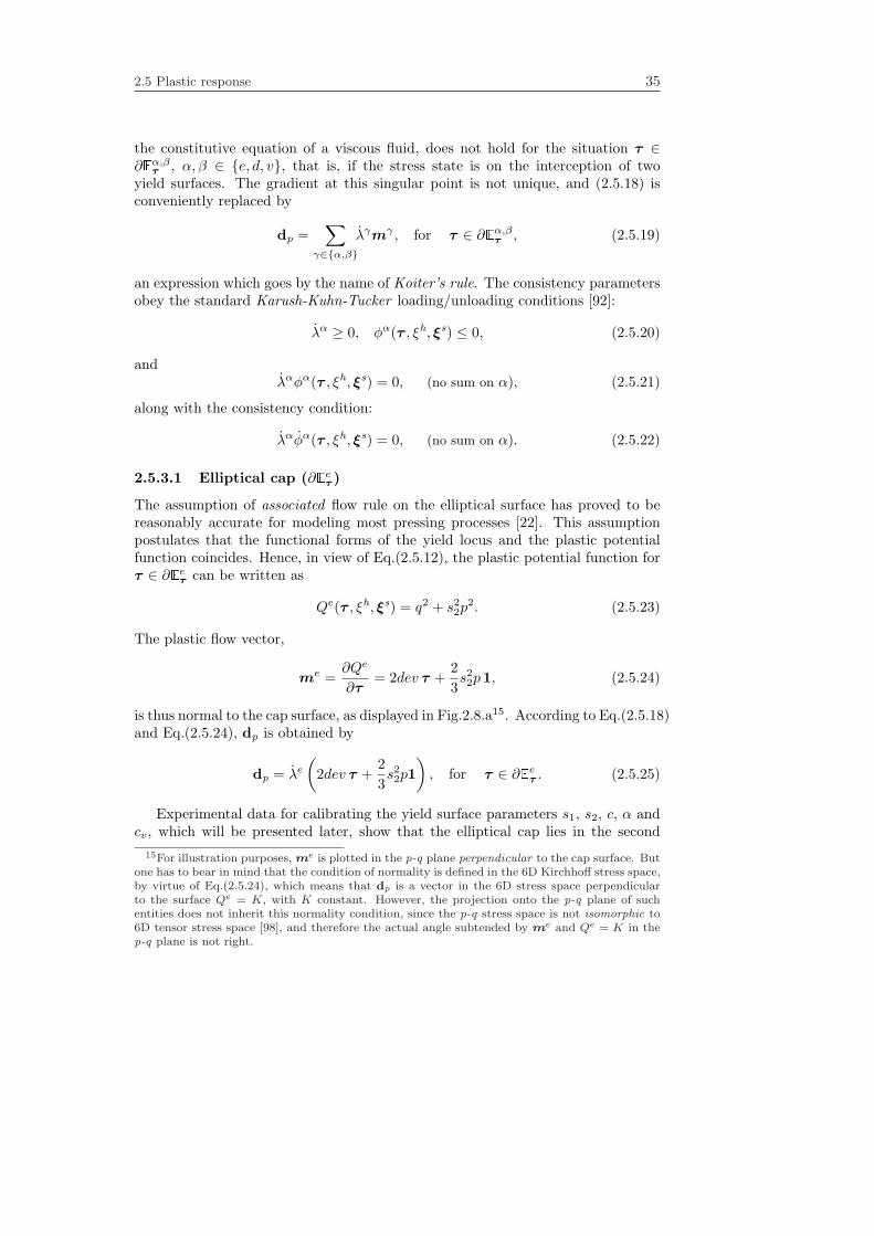
2.5 Plastic response 35
the constitutive equation of a viscous fluid, does not hold for the situation τ ∈∂Eα,βτ , α, β ∈ e, d, v, that is, if the stress state is on the interception of twoyield surfaces. The gradient at this singular point is not unique, and (2.5.18) isconveniently replaced by
dp =∑
γ∈α,βλγmγ , for τ ∈ ∂Eα,βτ , (2.5.19)
an expression which goes by the name of Koiter’s rule. The consistency parametersobey the standard Karush-Kuhn-Tucker loading/unloading conditions [92]:
λα ≥ 0, φα(τ , ξh, ξs) ≤ 0, (2.5.20)
andλαφα(τ , ξh, ξs) = 0, (no sum on α), (2.5.21)
along with the consistency condition:
λαφα(τ , ξh, ξs) = 0, (no sum on α). (2.5.22)
2.5.3.1 Elliptical cap (∂Eeτ )
The assumption of associated flow rule on the elliptical surface has proved to bereasonably accurate for modeling most pressing processes [22]. This assumptionpostulates that the functional forms of the yield locus and the plastic potentialfunction coincides. Hence, in view of Eq.(2.5.12), the plastic potential function forτ ∈ ∂Eeτ can be written as
Qe(τ , ξh, ξs) = q2 + s22p2. (2.5.23)
The plastic flow vector,
me =∂Qe
∂τ= 2dev τ +
23s22p1, (2.5.24)
is thus normal to the cap surface, as displayed in Fig.2.8.a15. According to Eq.(2.5.18)and Eq.(2.5.24), dp is obtained by
dp = λe(
2dev τ +23s22p1
), for τ ∈ ∂Eeτ . (2.5.25)
Experimental data for calibrating the yield surface parameters s1, s2, c, α andcv, which will be presented later, show that the elliptical cap lies in the second
15For illustration purposes, me is plotted in the p-q plane perpendicular to the cap surface. Butone has to bear in mind that the condition of normality is defined in the 6D Kirchhoff stress space,by virtue of Eq.(2.5.24), which means that dp is a vector in the 6D stress space perpendicularto the surface Qe = K, with K constant. However, the projection onto the p-q plane of suchentities does not inherit this normality condition, since the p-q stress space is not isomorphic to6D tensor stress space [98], and therefore the actual angle subtended by me and Qe = K in thep-q plane is not right.

36 2. Continuum modeling of the powder behavior
q
p
(a)
q
p
(b)
ttrial
A
ttrial
B
tA
ˆd
Q K= ˆd
Q K=
Figure 2.8 Direction of the plastic flow. (a) Associated flow (ellipse) + linear plasticpotential function (b) Singularity at the vertex.
quadrant of the p-q plane (p < 0) for the whole range, supported by experiments,of such parameters. Stated otherwise,
τ ∈ ∂Eeτ ⇒ p < 0. (2.5.26)
A useful result can be extracted from this condition. Taking the trace of both sidesof Eq.(2.5.25), it yields
trdp = λe2s22p for τ ∈ ∂Eeτ . (2.5.27)
Hence, by virtue of condition (2.5.26) and the positiveness of λe, expression (2.5.27)reveals that plastic strain increments are compressive (trdp < 0) whenever yieldingoccurs in the stress range determined by the elliptic surface. Furthermore, it followsfrom the above condition and from Eq.(2.5.2) that the general expression for theevolution of the hardening variable ξh takes the form
ξh = −ξhλe2s22p. (2.5.28)
Thus, stress states on ∂Eeτ are unequivocally correlated with hardening behavior,being precluded the occurrence of a different phenomenological trend.
2.5.3.2 Drucker-Prager yield surface (∂Edτ )
Whereas the hypothesis of associated flow rule is generally accepted, and almosttacitly invoked, in the case of the elliptical cap ∂Eeτ , the direction of dp when thestress point lies on the Drucker-Prager envelope ∂Edτ is plagued by much contro-versy. Some authors simply extend the validity of the associative assumption andconsider that dp is normal to the failure line [20, 90, 33]. However, this hypothesisis clearly at odds with reality (it over-predicts the dilatational response), as expe-rimental studies carried out by Pavier [83] and Sinka [94] evidence. These studies

2.5 Plastic response 37
reveal that the direction of dp is only adequately described by the normality con-dition in the cap portion ∂Eeτ . As the stress state approaches the interceptionwith the Drucker-Prager envelope, the plastic strain increment becomes steeper.Eventually, at the interception point ∂Ee,dτ , dp turns vertical and the nature ofthe plastic flow ceases to be compressive. Furthermore, according to Pavier [83],dp maintains this vertical orientation in the Drucker-Prager stress range, or, inother words, the material flows at constant volume when yielding occurs on theDrucker-Prager surface ∂Edτ , being precluded the occurrence of dilatation. Moti-vated by these observations, some authors have favored the assumption of isochoric(trdp = 0) plastic flow on the failure surface [17, 109].
Apart from the above mentioned studies, the characterization of the plasticflow in the failure region does not feature in the literature on powder compactionmodeling, whereby recourse is to be made to models developed for other granularmaterial, such as soils, to further guide our analysis in this respect. Frictionaleffects in a granular material are manifested by volumetric dilatancy, especially inthe low confinement regime [105]. Therefore, it is plausible to expect also a similarbehavior, in some extent, in the powder. To accommodate this dilatancy in theflow rule, when using the Drucker-Prager yield criterion (2.5.13), the most commonplastic potential function employed is formulated as
Qd = q + βp, (2.5.29)
and the corresponding flow vector is given by
md =∂Qd
∂τ=
dev τ
‖dev τ‖ +13β1. (2.5.30)
Note that the equation Qd = K, with K constant, also defines a straight line, asthe yield criterion (2.5.13), in the p-q plane. The material parameter β, the slopeof such line, is often called dilatancy factor [60], and it represents the ratio of thevolumetric and shear (deviatoric) part of the plastic rate of deformation, i.e.
β =trdp
‖dev dp‖ . (2.5.31)
With a vanishing dilatancy factor (β = 0), the isochoric plastic flow is recovered,and associated plasticity results if β = α.
Nevertheless, it has been long known that, when a backward Euler integra-tion scheme is applied to solve the resulting differential equations, the use of theplastic potential function (2.5.29) gives rise to numerical difficulties. A completeunderstanding of the reasons behind such difficulties requires some notions of thestructure of the integration scheme. Skipping for now the derivation details, whichwill be addressed in Chapter 3, we can roughly say that the stress update algorithmresulting from this time-integration procedure is based on, first, the computationof a certain elastic predictor or trial stress, by assuming elastic behavior through-out a given step. If such trial stress lies outside the elastic domain, that is, if itviolates the algorithmic counterpart of Eq.(2.5.20), then the updated stress is ob-tained by projecting the trial state back to the yield surface (return map). The

38 2. Continuum modeling of the powder behavior
return direction depends basically on the direction of the plastic flow vector md,but they do not necessarily coincide. For illustration purposes, however, supposethat the return direction is aligned with md, and furthermore, that the yield sur-face is fixed. In Fig. 2.8.b, the orientation of md, which is constant, is sketched fora value of the dilatancy factor β < α. The return map would bring a trial stresssuch as τ trA , lying on the left hand side of the Drucker-Prager apex (intersectionof ∂Edτ with the abscissa), back to a point τA ∈ ∂Edτ . Difficulties are encountered,however, when the trial state lies in the shaded region on the right hand side ofthe apex (Fig. 2.8(b)). Clearly, the return direction that would project the trialstress τ trB back to the yield surface (to the apex) is not derived from the potentialfunction (2.5.29). This singularity might seriously affect the rate of convergenceof the iterative scheme which accompanies the incremental analysis, and hence therobustness and reliability of the numerical predictions.
Parabolic plastic potential functionIt can be readily concluded from the foregoing explanation that the root cause
of these difficulties is the non-smoothness of the plastic potential surface definedby (2.5.29) at the apex. The solutions proposed to alleviate this shortcoming arebasically of two types. On one hand, one may introduce an additional cap to “roundoff” the linear potential function at that point [32]. On the other hand, one mayresort to a different potential function meeting the requirement of smoothness atthe apex [105, 56]. Here the latter approach is adopted. The proposed parabolicplastic potential function, expressed as
Qd(τ , ξh, ξs) = q2 + β(ξh, ξs) p, (2.5.32)
with β > 0, is adequate to this end, since the corresponding flow vector:
md =∂Qd
∂τ= 2 dev τ +
13β1, (2.5.33)
is horizontal, in the p-q plane, at the apex (q = 0), and, consequently, the normalsto the potential surface cover all possible return directions.
The equation Qd = K, with K constant, defines a parabola in the p-q plane,hence the name of parabolic potential. The use of parabolic plastic potential func-tions can be traced back to the work of Willam et al.[34], and it is frequently utilizedfor the characterization of failure mechanisms for cohesive frictional materials [38].However, there is a fundamental difference between these constitutive models andthe one presented here. Willam’s model is a parabolic extension of both the yieldcriterion and the potential function, i.e., both the yield and the potential functionsare parabolic-shaped. The essence of our approach, by contrast, is to introduce aparabolic potential function, but maintaining the classical (linear) Drucker-Prageryield criterion (see Fig. 2.9). In this way, the singularity at the vertex is circum-vented and, at the same time, the simplicity and the computational convenienceof using a linear yield criterion is retained. It should be remarked that claimswith regard to the necessity of “rounding off” the Drucker Prager yield surface atthe apex for avoiding the singularity are unfounded, and might be ascribed to anover-exposure to associated plasticity.

2.5 Plastic response 39
q
pParabolic potential surface
Linear yield surface
dQ K=
Figure 2.9 Parabolic plastic potential surface, for γ close to zero.
Thermodynamic consistency
With such an approach, which appears to be a truly novel element of the presentdevelopment, one is faced with the unexplored task of determining a functional formfor the state function β = β(ξh, ξs). In order to avoid thermodynamically unrea-sonable results, the functional form of β must be consistent with the dissipationinequality (2.3.7), which, for the case in which only the Drucker-Prager yield surfaceis active (ξh = 0), reduces to
D = τ : dp − ψs = τ : dp − ∂ψp
∂ξsξs ≥ 0. (2.5.34)
As outlined in section (2.3), the term ψs is associated with a release of energy,i.e. ψs ≤ 0. Hence, the worst conceivable circumstances for the satisfaction ofinequality (2.5.34) correspond to the case ψs = 0. A sufficient condition for ensuringthe positiveness of D is therefore
τ : dp ≥ 0. (2.5.35)
According to Eq.(2.5.18) and Eq.(2.5.33), the plastic rate of deformation tensortakes the form
dp = λd(2 dev τ +13β1), for τ ∈ ∂Edτ . (2.5.36)
with λd ≥ 0. Substitution of (2.5.36) in (2.5.35) leads to:
τ : dp = λd(
2dev τ : τ +13β1 : τ
)= λd
(2q2 + βp
) ≥ 0. (2.5.37)

40 2. Continuum modeling of the powder behavior
The bracketed term of Eq.(2.5.37) is expressible as a polynomial in q by enforcingthe yield condition (2.5.13):
τ : dp = λd(
2q2 − β
αq +
β
αc
). (2.5.38)
It is straightforward to show that the above inequality is fullfiled for all q ≥ 0provided that (
β
α
)2
− 8cβ
α≤ 0 ⇒ β ≤ 8cα. (2.5.39)
It follows from the above condition, hence, that a logical choice for the functionalform of β is
β = γ cα, with 0 ≤ γ ≤ 8. (2.5.40)
The material parameter γ controls the plastic dilatancy, and it is considered con-stant over the whole stress range. In order to reproduce the behavior described byPavier [83], γ is set to values close to zero, so that the the plastic flow is practicallyisochoric in the whole range of stresses, except in a small neighborhood at the apex,wherein the flow vector rotates until becoming purely dilatational for q = 0 (seeFig. 2.9).
2.5.3.3 Von Mises surface (∂Edτ )
The Von Mises yield surface represents a theoretical threshold in stress space be-yond which inelastic volumetric deformation ceases and only deviatoric flow canoccur. In this aspect, the behavior of the powder at this stress range parallels thatof the fully dense material. The direction of plastic flow is obtained, thus, from thefollowing potential function:
Qv(τ ) = q2. (2.5.41)
The plastic flow vector is, hence, purely deviatoric:
mv =∂Qv
∂τ= 2dev τ . (2.5.42)
Note that the definition (2.5.2) of internal hardening variable indicates thathardening is precluded when yielding takes place at ∂Evτ :
ξh = −ξhtrdp = 0. (2.5.43)
2.5.4 Hardening laws
Using the standard chain rule for the partial derivatives of a function of severalvariables, we can write
s1 =
s1h︷ ︸︸ ︷∂s1∂ξh
ξh +
s1s︷ ︸︸ ︷∂s1∂ξs
ξs = s1h + s1s . (2.5.44)

2.5 Plastic response 41
The same holds for the other state variables:
s2 =∂s2∂ξh
ξh +∂s2∂ξs
ξs = s2h + s2s , (2.5.45)
c =∂c
∂ξhξh +
∂c
∂ξsξs = ch + cs , (2.5.46)
α =∂α
∂ξhξh +
∂α
∂ξsξs = αh + αs , (2.5.47)
cv =∂cv∂ξh
ξh +∂cv∂ξs
ξs = cvh + cvs (2.5.48)
Here the subscripts h and s denote hardening and softening respectively. Thisdecomposition is particularly appealing since it permits a separate description ofboth phenomena. Relationships between the hardening counterparts of each statevariable, i.e. ch, and the internal hardening variable are called hardening laws, ch =c(ξh)ξs=cte. Conversely, softening laws are relations of the type cs = c(ξs)ξh=cte, i.e.relating the softening counterpart of the state variables and the internal softeningvariables. Attention is restricted in this section to describe the former group ofrelationships, the hardening laws. Dependence of the elastic parameters on ξh isalso addressed herein.
2.5.4.1 Elliptical surface parameters (s1h, s2h)
Major axis (s1h)In Section B.1 of Appendix B, some useful expressions are drawn from an ap-
proximated (ignoring elastic effects) analysis of triaxial loading on a cylindricalspecimen. According to these expressions, the functional form of s1h(ξh) can beobtained by monitoring the pressure required for achieving different levels of den-sity16 when a specimen is compacted isostatically, or, in other words, it correspondsto the hydrostatic yield stress in compression. For iron-based powders, the expres-sion of s1h is found to be given by [83]:
s1h = Jscy1h =ρ0
ρAs1
(ln
(1− ηapp1− ξh
)) 1Ns1
. (2.5.49)
The parameters As1 and Ns1 are empirically adjusted for each alloy composition.The relative apparent density ηapp is defined as
ηapp =ρappρth
, (2.5.50)
where ρapp and ρth are, respectively, the apparent and theoretical density of thepowder. Note that scy1h denotes the mayor axis of the elliptical yield surface in the
16In conformance with definition (2.5.1) of hardening internal variable, density herein refers tothe overall density of the specimen measured after being extracted from the mold.

42 2. Continuum modeling of the powder behavior
Cauchy stress space. The Jacobian determinant J is introduced to put in correspon-dence experimental (true) stress data with Kirchhoff stress values. For purposesof simplification in the subsequent numerical integration, it proves advantageousto invoke again the assumption of negligible elastic strains and approximate, inexpression (2.5.49), the Jacobian determinant as
J =ρ0
ρ=ρ0/ρthρ/ρth
≈ η0ξh, (2.5.51)
whereη0 =
ρ0
ρth. (2.5.52)
Approximation (2.5.51) permits to cast s1h solely in terms of the internal hardeningvariable ξh:
s1h(ξh) =η0ξhAs1
(ln
(1− ηapp1− ξh
)) 1Ns1
. (2.5.53)
0.4 0.5 0.6 0.7 0.8 0.9 10.30
100
200
300
400
500
600
hx
Hydr.
yie
ld s
tress (
Mpa)
1cy h
s
Internal hardening variable
happ
Curve fit
Experiment (Pavier)
Figure 2.10 Hydrostatic yield stress in compression scy1h versus internal hardening vari-
able ξh. Stress data represented in Cauchy (true) stress space. Experimental data fromisostatic compression tests carried out by Pavier [83] on Distaloy AE powder specimens.
In figure 2.10, values of scy1h, obtained in hydrostatic compression tests carried outby Pavier [83], are plotted versus ξh for an iron base powder (Distaloy AE) withparameters ρ0 = 3.04g/cm3 and ρth = 7.33g/cm3. Fitting Eq.(2.5.49) to theseexperimental data we have As1 = 95.4439MPa and Ns1 = 0.6506. The curve fitbears close similarity to a typical compressibility curve (see figure 2.1.c), strictly itsinverse, with a steadily increasing slope, in such a way that the hydrostatic yieldstrength asymptotes to infinity when ξh approaches unity.
Eccentricity (s2h)
The state variable s2h is related to the radial to axial stress ratio ktr, also known

2.5 Plastic response 43
as pressure transmission coefficient, through the following expression:
s2h(ξh) =
√3(1− ktr(ξh))1 + 2ktr(ξh)
, (2.5.54)
as deduced in Appendix B.1. In figure 2.11, radial to axial stress ratio measures,collected by Sinka [94] on a Distaloy AE powder specimen, are displayed for severalrelative (inelastic) densities. Two regions can be distinguished in this plot. Experi-mental data points from approximately ξh = 0.65 show a clear increasing tendency,whereas data for low relative densities (0.55 − 0.65) are widely scattered. Thesediscrepancies at low densities are attributable to the lack of accuracy in monitoringstress values at this density range on powder materials. Furthermore, experimentalinformation is available only for ξh > 0.55, hence the behavior for densities closeto ηapp is also uncertain.
0.4 0.5 0.6 0.7 0.8 0.9 10.1
0.2
0.3
0.4
0.5
0.6
0.7
0.8
0.9
hxInternal hardening variable
Radia
l to
axia
l str
ess r
atio
,tr
k
trkhapp
h
0trk
Curve fit
Experiment (Sinka)
Figure 2.11 Radial to axial stress ratio versus internal hardening variable ξh. Expe-rimental data obtained from simulated closed die compactions conducted by Sinka et al.[94] on Distaloy AE powder specimens.
In view of this lack of experimental evidence, it proves advantageous to employpredictions of micromechanical models for the early stages of compaction. Thosepredictions assert that the initial radial to axial stress ratio is ktr0 = 1/3 [22].Note that this assertion is at odds with other descriptions found in the literature.Cante et al.[17] claimed that the eccentricity of the elliptical cap approaches zero,or equivalently ktr → 1, at values close to the apparent density. However, thisassumption implies that the bulk powder cannot sustain any shear stress or, equiv-alently, it ascribes a fluid-like behavior to the cohesionless powder, which is nottotally realistic.
The following empirical equation is proposed here for the radial to axial stressratio (see figure 2.11):

44 2. Continuum modeling of the powder behavior
ktr(ξh) =ktr0, if ξh ≤ ηktr
,(ξh − ηktr )(Aktrξ
h +Bktr ) + ktr0, if ξh > ηktr .(2.5.55)
Note that the proposed functional form for ktr acknowledges the abovementionedfacet of powder characterization by fixing ktr in a constant value ktr0 = 1/3 fordensities below ηktr
. Calibration of the parameters for this particular Distaloy AEalloy gives Aktr = 1.074, Bktr = 0.242 and ηktr = 0.635. In figure 2.12, the curves2h = s2h(ξh) obtaining by introducing Eq.(2.5.55) in Eq.(2.5.54) is shown.
hx
0.4 0.5 0.6 0.7 0.8 0.9 1
0.5
0.6
0.7
0.8
0.9
1
1.1
Internal hardening variable
Elli
pse
ecce
ntr
icity,
2h
s
Figure 2.12 Values of the elliptical cap yield surface eccentricity (s2h), obtained by sub-stituting the fitting equation (2.5.55) for ktr in Eq.(2.5.54), versus the internal hardeningvariable ξh.
2.5.4.2 Drucker-Prager yield surface parameters (ch, αh)
The location of the Drucker-Prager failure line in the p−q plane for several densitiesis obtained by performing, at least, two sets of fracture tests, namely a uniaxialcompression test and and a Brazilian disc or diametral compression test. Thefailure line is then plotted by connecting fracture stress points corresponding tothe same density.
Cohesion (ch)
Coube [25] followed the above procedure to collect values of cohesion, shown infigure 2.13, and values of the parameter of internal friction αh, displayed in figure2.14.a, as a function of ξh for a Distaloy AE powder. The curve fit for the cohesionis given by the equation17
ch(ξh) =
√23η0ξhccyh =
√23η0ξhAche
Bchξh
. (2.5.56)
17Notice that the factorp
2/3 accounts for the fact that the deviatoric stress q = ‖dev τ‖ isnot a Von Mises effective stress measure.

2.5 Plastic response 45
hx
0.4 0.5 0.6 0.7 0.8 0.9 1
Internal hardening variable
0
10
20
30
40
50
60
cy
hc
, C
ohesio
n (
)M
Pa
Experiment (Coube)
Curve fit
Figure 2.13 Cohesion, in Cauchy (true) stress space, against internal hardening vari-
ables ξh. Experimental data obtained by experiments carried out by Coube [25] on Dis-taloy AE powder specimens.
Calibration of this equation for the data shown in figure 2.13 yieldsAch = 0.001MPaand Bch = 11.2368.
Inspection of the cohesion ch, which can be regarded as the shear strength underzero hydrostatic stress, and the hydrostatic yield stress in compression s1h attainedat a given value of the relative density, say ξh = 0.9, indicates that the greencompact is notably weaker in tension/shear than in compression, up to a factors1h/ch ≈ 24.
Internal friction parameter (αh)Two curve fits for the parameter of internal friction αh(ξh) are shown in figure
2.14.a. From a regression analysis standpoint, the best fit is obviously the linear one.From a physical point of view, however, the values of αh predicted by this linear fitin the range of low densities (ξh < 0.65) are meaningless. The reasoning underlyingthese unsatisfactory predictions is that, in order to ensure a finite value for the yieldstress in uniaxial compression, the parameter of internal friction cannot exceed theslope (in absolute value) of the stress path in the p − q plane corresponding to auniaxial compression test (see figure 2.14.b) [60]. It can be easily deduced that theslope of the uniaxial compression stress path is −√6, hence we have the condition
αh <√
6. (2.5.57)
For ξh = 0.6, we can see in figure 2.14.a that the linear fit estimates αh ≈√2/3 · 3.05 = 2.49, which is greater than
√6 ≈ 2.45.
Thus, the appropriate fit is a constant one, also shown in figure 2.14.a:
αh = αh0, (2.5.58)
with αh0 =√
2/3 · 2.81 = 2.29.

46 2. Continuum modeling of the powder behavior
0.6 0.65 0.7 0.75 0.8 0.85 0.95 10.9
2.7
2.8
2.9
3
3.1
2.6
hx
Experiment [Coube]
Curve fit (linear)
Curve fit (constant)
Pa
ram
. o
f in
t. f
rictio
n,
3 2h
a
6atan( )h
aatan( )
(a)
Internal hardening variablep
q
(b)
Figure 2.14 (a) Parameter of internal friction αh versus internal hardening variable
ξh. Experimental data obtained by experiments carried out by Coube [25] on DistaloyAE powder specimens. (b) Representation of the stress path corresponding to a uniaxialcompression test. The parameter of internal friction αh cannot exceed the slope of suchstress path.
As in the case of s2h, empirical observations concerning the evolution of αh
for the range of low densities are not available, since an unavoidable requirementfor undertaking fracture tests is that the specimen must posses some degree ofconsolidation, so as to be ejected from the die cavity without rupture. It seemsmore suitable in this regard to undertake flowability tests and other experimentsin which the behavior of the powder in its cohesionless state can be characterized.Exploring such subject goes beyond the scope of this work. Hence, the assumptionof a constant parameter of internal friction over the whole range of density will beadopted.
2.5.4.3 Von Mises yield surface parameter (cvh)
Experimental isodensity yield stress points in p−q space are presented in figure 2.15.The tests for obtaining such information were conducted by Pavier[83] by subject-ing cylindrical powder (Distaloy AE) specimens to different triaxial loading paths(consolidated and over-consolidated compression tests). In figure 2.15.a, isodensitycontours are constructed by using an elliptical cap together with a Drucker-Pragerfailure line. On the other hand, in figure 2.15.b, isodensity contours are modifiedby introducing an additional horizontal straight line (Von Mises surface).
It is readily seen here that the best fit to the stress data points is providedby the isodensity contours plotted in figure 2.15.b, in which the Von Mises yieldsurface is considered. The failure line and the hardening cap on their own (seefigure 2.15.a) overpredict the yield stress of the material in the vicinity of the their

2.5 Plastic response 47
intersection, to such an extent that the physically unattainable threshold σy (theyield strength of the full dense material) is clearly exceeded at a relative densityη = 0.982 .
100
200
300
400
0-100-200-300-400-500-600-600-700
Cauchy Hydrostatic Stress, MPa
Ca
uch
y E
ffe
ctive
Str
ess,M
Pa
0.941h=
0.955h=
0.969h=
0.982h=
ys
100
200
300
400
0-100-200-300-400-500-600-600-700
Cauchy Hydrostatic Stress, MPa
Ca
uch
y E
ffe
ctive
Str
ess,M
Pa
0.941h=
0.955h=
0.969h=
0.982h=
0.9410.955
0.9690.982
0.9820.969
0.9550.941
ys
Figure 2.15 Experimental data from consolidated and over-consolidated compressiontests (Pavier [83]) on Distaloy AE powder specimens. Isodensity contours employing (a)Drucker-Prager + Elliptical cap, (b) Drucker-Prager + Elliptical cap + Von-Mises
The comparison displayed in figure 2.15 conveys the relevance of the role playedby the Von-Mises yield surface in the later stages of compaction. To proceed withthe calibration of the hardening counterpart of the Von Mises parameter, cvh, weidentify, as usual, relative density and hardening internal variable (ξh ≈ η), on thebasis that the slight difference between them (due to volumetric elastic strain) isof the same order as the measurement error. In figure 2.16.b, the values of cvhresulting from the fit shown in figure 2.15.b are plotted versus ξh . The curveABC represents the path traced by the deviatoric stress measure qcyint (see figure2.15.a) at the intersection of the Drucker-Prager and the elliptical cap (∂Ed,eτ ). Thecurve BD is the quadratic fit to the data points obtained from figure 2.15.b. Inorder to put the evolution of cvh in a mathematically suitable form, we assumethat the curve cvh = cvh(ξh) is composed of the branches AB and BD. Fromthe apparent density up to ηv0, the Von Mises surface is reduced to a point, the

48 2. Continuum modeling of the powder behavior
intersection ∂Ed,eτ . In practice, this means that the Von Mises yield surface is notconsidered for computational purposes for ξh < ηv0. It is only for densities aboveηv0 when it actually comes into play. The following empirical correlation reflectsthese considerations:
100
150
200
250
350
400
300
450
500
0.8 0.84 0.88 0.92 0.96 1
ys
cy
vhc
int
cyq
0vh
hx
A
Data from isodensity contourn fit
Curve fit,cy
vhc
Intersection ellipse-DP, int
cyq
Cauchy Hydrostatic Stress
Cauchy E
ffective S
tress
Ca
uch
y E
ffe
ctive
Str
ess (
)M
Pa
B
C
D
Figure 2.16 (a) Definition of qcyint as the deviatoric stress measure at the intersection of
the Drucker-Prager and the elliptical cap (∂Ed,eτ . (b) Von Mises parameter cvh vs internalhardening variable ξh. The curve AC corresponds to qcyint = qcyint(ξ
h), whereas BD is thequadratic fit to the data points obtained from the isodensity contours shown in 2.15.b.
cvh(ξh) =
qint =√
23η0ξhqcyint, if ξh ≤ ηv0,√
23η0ξhσy(1−Acvh(ξ
h −Bcvh)(1− ξh)), if ξh > ηv0.
(2.5.59)
The fitted parameters for the Distaloy AE powder are Acvh = 58.160, Bcvh =0.8252, σy = 370MPa and ηv0 = 0.92.
The relative merits of employing an additional surface, to enhance the calibra-tion of experimental stress data point, instead of, say, a unique yield function, willbecome manifest later. Indeed, inspection of Eqs. (2.5.18), (2.5.36) and (2.5.42)reveals that the plastic flow vector on ∂Edτ , ∂Eeτ and ∂Evτ , respectively, is linearin τ , a feature that will offer a remarkable aspect of simplicity in the subsequentnumerical integration.
2.5.4.4 Elastic parameters (Ee,νe)
As mentioned in section (2.4), the neglect of anisotropy effects renders the elas-tic response governed only by two parameters, the Young’s modulus Ee and thePoisson’s ratio νe. Experimental measures of the Poisson’s ratio show a high vari-ability with density, but without a clear trend [83]. This high variability is due tothe difficulty in measuring accurately stresses in the radial direction. Hence, the

2.5 Plastic response 49
hypothesis of constant Poisson’s ratio, of a value equal to that of the fully densematerial (νe = 0.29), is regarded as a reliable approximation.
Experimental data of Young’s Modulus as a function of density, provided byPavier [83], are shown in figure 2.17. The following exponential fit is proposed
Ee(ξh) =η0ξhE0e
BE(ξh−η0), (2.5.60)
with E0 = 1360.92 MPa and BE = 8.82 for a Distaloy AE18.
hxInternal hardening variable
0.55 0.60 0.65 0.7 0.75 0.8 10.85 0.9 0.950
50
100
150
200
250
(Cauchy)
Young
’s M
odulu
s (
Gpa)
Experiment [Pavier]
Curve fit
Figure 2.17 Young’s Modulus Ee vs internal hardening variable ξh. Experimental dataobtained by tests conducted by Pavier [83] on Distaloy AE powder specimens.
In using the above expression, we should bear in mind that this experimentalcorrelation was obtained in triaxial tests by subjecting a cylindrical specimen tocycles of axial loading and unloading at different levels of (constant) radial pressure.Although it was observed that the relation between increments of axial stress andaxial strain depends on the level of radial pressure, Pavier [83] suggested that, asa first approximation, this dependence may be disregarded.
On the other hand, by measuring the velocity of sound in the pressing directionon previously compacted Distaloy AE cylindrical specimens, Coube [25] concludedthat an estimation for the elastic modulus in a stress-free situation is given by thefollowing linear equation
Ee(ξh) =η0ξh
(YE1 + YE2ξh), (2.5.61)
where YE1 = −16383.47MPa and YE2 = 39073.95MPa.In view of the experimental procedures from which Eqs. 2.5.60 and 2.5.61
are drawn, it seems more reasonable to employ Pavier’s empirical law 2.5.60 in de-scribing the elastic behavior in situations of confinement, whereas, in circumstancescloser to unstressed configurations, Coube’s relation (Eq.(2.5.61)) seems more ade-quate. A comparison of the values obtained by evaluating 2.5.60 and 2.5.61 at, say
18Note that the elastic free energy function (2.4.1) was defined per unit reference volume, hencethe necessity of the (approximated) Jacobian factor η0/ξh.

50 2. Continuum modeling of the powder behavior
ξh = 0.9, reveals that the Young’s Modulus predicted by the former is up to fivetimes larger than the one predicted by the latter. Obviously, these two notoriouslydifferent estimations can be reconciled by using a unique non-linear elastic law, asthe one presented in Mosbah [69], in which the elastic secant modulus Ee (the de-nomination “Young’s modulus” would be a misnomer in this case) depends furtheron the stress state. Such generality, however, would complicate substantially thesubsequent numerical integration.
2.5.5 Softening laws
The softening constitutive laws are relationships between the softening counterpartof the state variables defining the size, shape and location of the yield condition,and the as yet unspecified set of internal softening variables ξs. Each affine trans-formation of the surfaces defining the yield condition in stress space is associatedwith a particular physical meaning. On this basis, we shall discern which variablesshould come into play for achieving a sufficient degree of realism, and, on the otherhand, which can be disregarded. Note that the number of relationships that can beconsidered is constrained by the availability of experimental data to support suchrelations.
2.5.5.1 Elliptical surface parameters (s1s, s2s)
It will be assumed that the compressive strength of the material remains unalteredin the course of failure events, i.e.:
s1s = 0 → s1(ξh, ξs) = s1(ξh) = s1h(ξh), (2.5.62)
s2s = 0 → s2(ξh, ξs) = s2(ξh) = s2h(ξh). (2.5.63)
Hence, the shape and size of the elliptical cap are completely determined by theinternal hardening variable ξh. At first sight, this hypothesis may appear toostringent from a physical standpoint. However, from a practical point of view, forreplicating the behavior of interest insofar as determination of cracks is concerned, itsuffices to account for the decay of mechanical strength in the tensile/shear regime,since the compact is more prone to failure in the pressure release and ejection stages,when these conditions prevail. Furthermore, the benefits arising in the subsequentnumerical integration of the constitutive equation, due to the simplicity affordedby this assumption, outweighs any slight lack of accuracy that might result.
2.5.5.2 Von-Mises yield surface parameter (cvs)
The Von Mises yield surface only plays an active role under circumstances of highdegree of confinement. Upon pressure release, the stress state at every point ofthe compact moves away from the cap and the Von Mises yield surfaces to thetensile/shear region. It seems reasonable, therefore, to disregard also the influence,as far as failure analysis is concerned, of the Von Mises yield surface. This impliesto extend the hypothesis made above for the state variables s1 and s2, and assumethat
2.5 Plastic response 51
cvs = 0 → cv(ξh, ξs) = cv(ξh) = cvh(ξh). (2.5.64)
i.e. the Von Mises parameter cv is insensitive to changes of the softening internalvariable ξs.
We must note emphatically that a general constitutive softening law cvs =cvs(ξs) can be accommodated in the formulation without any conceptual differ-ence. The guidelines would be the same as the ones that we shall describe in theensuing discussion (Drucker-Prager yield surface parameters). The only substantialchange would arise in the numerical integration, since the integration of any con-stitutive law involving softening poses a great mathematical challenge, as it will bediscussed in Chapter 3. Besides, any constitutive relation must be substainted bythe corresponding experimental tests, and empiric observations, concerning frac-ture energy measurements, in tests in which the stress path involves yielding onthe Von Mises surface are not available at present.
2.5.5.3 Drucker-Prager yield surface parameters (cs, αs)
We focus now on the details concerning the evolution of the Drucker-Prager failureenvelope in stress space when softening takes place. This surface bounds the tensileand shear, for low degree of confinement, regions, hence a decrease of mechanicalstrength is reflected by a motion towards the origin of the Drucker-Prager yieldsurface in the p-q plane. We shall assume that the uniaxial tensile strength, whichis related to the Drucker-Prager parameters through the expression
σt =
√32
√6c√
6 + α, (2.5.65)
(see figure 2.18) decays at the same rate as the cohesion c. It follows from Eq.(2.5.65),and considering relation (2.5.58), that this assumption is tantamount to assert theconstancy of α. Therefore, the parameter of internal friction α is independent ofboth ξh and ξs and α can be regarded as a material constant , i.e.
αs = 0 → α = αh0. (2.5.66)
Therefore, in view of Eqs. (2.5.62), (2.5.63), (2.5.64) and (2.5.66), the task ofestablishing the set of softening laws is reduced to find the relationship cs = cs(ξs).To take developments a step forward, we have first to specify the set of internalsoftening variables. As it was pointed out in Eq.(2.5.9), the assumption of strainsoftening is adopted, which means that the amount of softening depends only onthe length of the trajectory in the plastic strain space but not on the strain pathitself [53], i.e.:
ξs1 =∫ t
t0
‖dev dp‖ dt, for τ ∈ ∂Edτ ∪ ∂Ed,eτ ∪ ∂Ed,pτ , (2.5.67)
ξs2 =∫ t
t0
trdp dt, for τ ∈ ∂Edτ ∪ ∂Ed,eτ ∪ ∂Ed,pτ , (2.5.68)

52 2. Continuum modeling of the powder behavior
6
6
c
+a
c
p
q
p
q
(a) (b)
( )atan a
( )0 ,0h
c c= x
0s
x =
0c =O
T
0sx >s
x®¥
Figure 2.18 (a) Tensile region in the p-q plane. Path OT represents the (elastic) stresstrajectory in a uniaxial tensile test (b) Decrease of cohesion due to the accumulation ofplastic shear strain
or in rate form:
ξs1 = ‖dev dp‖, for τ ∈ ∂Edτ ∪ ∂Ed,eτ ∪ ∂Ed,pτ , (2.5.69)
ξs2 = trdp, for τ ∈ ∂Edτ ∪ ∂Ed,eτ ∪ ∂Ed,pτ . (2.5.70)
Note that in Eqs. (2.5.67) to (2.5.70), it is explicitly remarked that ξs1 and ξs2only evolve during intervals of plastic loading in which the stress state remains onthe Drucker-Prager failure line. Therefore, the rate form definitions (2.5.69) and(2.5.70) can be rephrased in terms of the plastic flow vector on ∂Edτ :
ξs1 = ‖dev dp‖ = 2λdq, (2.5.71)
ξs2 = trdp = λdγαc. (2.5.72)
In Eq.(2.5.46), it was assumed the additive decomposition of the cohesion rate,c = ch + cs. The usefulness of this decomposition will become apparent in thenumerical integration. A close inspection of the definitions of ξh, ξs1 and ξs2 revealsthat the simultaneous occurrence of both hardening and softening is only possiblewhen the stress state lies on the intersection ∂Ed,eτ of the elliptical cap and Drucker-Prager line, where precisely more numerical difficulties are encountered19. However,
19In the subsequent numerical integration, the coupling between hardening and softening when
the stress state is located at the intersection point ∂Ed,eτ will be eliminated by modifying theevolution equation for ξs1, that will take the form ξs1 = (1 − H(λe))(2λdq), where H(•) denotesthe Heaviside function. Hence, it will be assumed that the occurrence of softening is precluded
at ∂Ed,eτ .

2.5 Plastic response 53
for the sake of clarity, we preclude this possibility from our current analysis andpresume that yielding takes place only at ∂Edτ . Therefore, we can legitimately write
c = cs, → c(t) = c0 +∫ t
tis
csdt. (2.5.73)
where tis denotes the time at which yielding at ∂Edτ is initiated and c0 is thecohesion at this time:
c0 = c(ξh(tis), ξs10, ξs20). (2.5.74)
Observe that the initial cohesion c0 depends on the degree of hardening, character-ized by ξh(tis), achieved in previous compacting processes. If ξsβ(tis) = 0, β = 1, 2,the initial cohesion c0 coincides with the cohesion20 that one would obtain fromthe curve of virgin material ch(ξh).
We are now faced with the task of setting a correlation between cs and ξs.Motivated by the exponential structure of the majority of empirical hardening lawsseen in the previous section, the following softening law is adopted
cs(ξs1, ξs2) = c0(e
1c0
(H01(ξs1−ξs10)+H02(ξ
s2−ξs20)) − 1). (2.5.75)
Recall that we only have at our disposal experimental fracture energy values, mea-sured in a single test, for calibrating the parameters H01 and H02, hereafter re-ferred to as softening parameters. Thus, we are confronted with the dilemma ofwhether to neglect the influence of one of the internal variables or to calibrate oneof these parameters, say H01, and consider the other one as a dependent variableH02 = H02(H01). The dilemma can be resolved if we take into account the relativeinfluence of both internal variables in the material response. Dividing Eq.(2.5.72)by Eq.(2.5.71), we get
ξs2
ξs1= γ
αc
2q. (2.5.76)
It was set forth in section (2.5.3) that, in order to reproduce the behaviorobserved experimentally , the dilatancy parameter γ is set to values close to zero.This fact, according to Eq.(2.5.76), brings into prominence the effect of shear plasticstrain in the material response, i.e.:
ξs1 À ξs2. (2.5.77)
Therefore, it will be assumed that ξs2 = 0, and the set of internal softening variablesis reduced to the single scalar variable ξs = ξs1.
However, one has to be aware of the limitations imposed by hypothesis (2.5.77).Its validity hinges on assuming that q is greater, or of the same order, as c. Thiscondition, although seldom, may fail in some circumstances. For instance, in anhypothetical hydrostatic tensile test, in which the stress state is such that q = 0,variable ξs1 would not evolve, and hence no failure would be predicted unless thedegrading effect of dilatational deformations (ξs2) is acknowledged.
20In practice, (see Eq.(3.2.89) in chapter 3), we simply make c0 = ch.
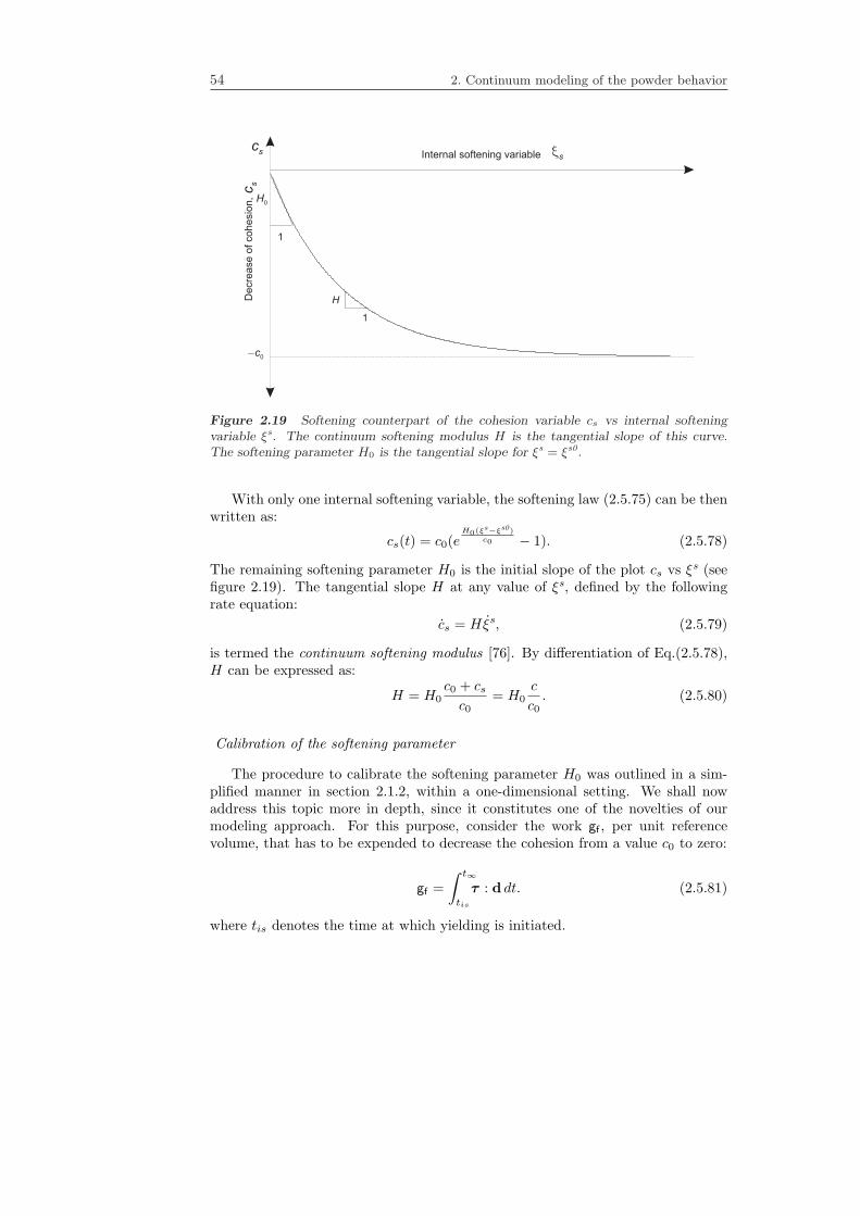
54 2. Continuum modeling of the powder behavior
Internal softening variable sxs
c
0c-
H
1
0H
Decre
ase o
f cohesio
n,
sc
1
Figure 2.19 Softening counterpart of the cohesion variable cs vs internal softeningvariable ξs. The continuum softening modulus H is the tangential slope of this curve.The softening parameter H0 is the tangential slope for ξs = ξs0.
With only one internal softening variable, the softening law (2.5.75) can be thenwritten as:
cs(t) = c0(eH0(ξs−ξs0)
c0 − 1). (2.5.78)
The remaining softening parameter H0 is the initial slope of the plot cs vs ξs (seefigure 2.19). The tangential slope H at any value of ξs, defined by the followingrate equation:
cs = Hξs, (2.5.79)
is termed the continuum softening modulus [76]. By differentiation of Eq.(2.5.78),H can be expressed as:
H = H0c0 + csc0
= H0c
c0. (2.5.80)
Calibration of the softening parameter
The procedure to calibrate the softening parameter H0 was outlined in a sim-plified manner in section 2.1.2, within a one-dimensional setting. We shall nowaddress this topic more in depth, since it constitutes one of the novelties of ourmodeling approach. For this purpose, consider the work gf , per unit referencevolume, that has to be expended to decrease the cohesion from a value c0 to zero:
gf =∫ t∞
tis
τ : d dt. (2.5.81)
where tis denotes the time at which yielding is initiated.

2.5 Plastic response 55
Using the additive decomposition of the rate of deformation tensor (Eq.(2.2.15)),we get
gf =∫ t∞
tis
τ : de dt+∫ t∞
tis
τ : dp dt. (2.5.82)
In virtue of Eq.(2.3.6), the first integral of the right hand side of the above equationtakes the form: ∫ t∞
tis
τ : de dt =∫ t∞
tis
∂ψe
∂ee: de dt. (2.5.83)
where ψe is the elastic free energy function, defined in Eq.(2.4.1). As proved inProposition A.1.1 of Appendix A, the rate of change of ψe is given by
ψe =∂ψe
∂ee: de +
∂ψe
∂ξhξh. (2.5.84)
Employing Eq.(2.5.84) in Eq.(2.5.83), we get∫ t∞
tis
τ : de dt =∫ t∞
tis
(ψe − ∂ψe
∂ξhξh) dt. (2.5.85)
We now suppose that, during intervals of plastic loading, the stress state remainson ∂Edτ . This implies that the cap yield surface is not active, λe = 0, and accordingto the rate equation (2.5.28), the internal hardening variable ξh does not evolve, i.eξh = 0. This observation permits to simplify Eq.(2.5.85) and omit the hardeningterm, resulting:
∫ t∞
tis
τ : de dt =∫ t∞
tis
ψe dt = ψe(ee(t∞))− ψe(ee(tis)). (2.5.86)
Assuming that the initial elastic strains are zero, we have
ψe(ee(tis)) = ψe(0) =12ee : ce : ee = 0. (2.5.87)
The term ψe(ee(t∞)) vanishes if we presume that the stresses are fully released attime t∞, i.e.:
ψe(ee(t∞)) =12ee(t∞) : ce : ee(t∞) =
12ee(t∞) :
0︷ ︸︸ ︷τ (t∞) = 0. (2.5.88)
Then, Eq.(2.5.82) reduces to the integral over the interval [tis, t∞] of the rateof plastic work (per unit reference volume):
gf =∫ t∞
tis
τ : dp dt. (2.5.89)
Using the flow rule (2.5.36), the above equation is rephrased as:
gf =∫ t∞
tis
λd(2q2 + γαcp) dt. (2.5.90)

56 2. Continuum modeling of the powder behavior
Employing Eqs. (2.5.71), (2.5.79) and (2.5.80), the plastic multiplier λd can beexpressed in terms of the cohesion variable and the norm of deviatoric stress:
λd =ξs
2q=
c02H0cq
c. (2.5.91)
Substitution of Eq.(2.5.91) in Eq.(2.5.90) yields
gf =∫ t∞
tis
c02H0cq
(2q2 + γαcp)c dt
=c0
2H0
∫ 0
c0
2q2 + γαcp
cqdc.
(2.5.92)
To proceed with the integration of (2.5.92), we need an additional ingredient:the path followed by the stress state during the process. This ingredient, in con-junction with the yield condition, permits the expression of the integrand of (2.5.92)as a function of the cohesion21.
We turn now our attention to describe the diametral compression test thatwill allow us to calibrate parameter H0. These tests were carried out by Jonsen[50] on Distaloy AE powder cylindrical specimens, previously compacted at variousdensities, by applying two diametrically opposite forces (see figure 2.20.a). Theseforces induce at the center of the disc a tensile stress state which eventually leadsto the initiation of a crack that propagates rapidly along the loaded diameter. Thesolid curve of the force vs displacement graph displayed in figure 2.21.a correspondsto the force monitored during the test until the specimen fractures. The area underthis curve encompasses not only the irretrievable energy consumed in the formationof the diametral crack, but also the recoverable elastic energy. In order to purge thisrecoverable contribution from the balance of energy, an additional test is needed.The specimen is split into two halves (see figure 2.20.b) and its response is evaluatedunder the same experimental conditions as in the previous test. The result of thisadditional experiment is the dashed curve also shown in figure 2.21.a. Finally, theenergy W required to produce such a crack is grossly estimated as the shaded areaenclosed by the solid and dashed lines.
As discussed in section 2.1.2, the fracture energy, denoted by Gf , is a measure ofthe energy required for the formation of a unit of fracture surface. Thus, fractureenergy values are obtained by simply dividingW by the area Af of material affectedby the crack (see figure 2.21.b). Experimental results for each relative density areshown in figure 2.22. An exponential equation seems to provide a good fit to thesedata:
G(dct)f (ξh) =
η0ξhAGf
eBGfξh , (2.5.93)
with AGf= 0.1487 J/m2 and BGf
= 9.5102. 22.
21Observe that this path dependence is an inherent property of materials with different behaviorin tension and compression. A classical pressure-independent Von Mises plasticity model, forinstance, would not exhibit this path dependence, as it may be deduced from Eq.(2.5.92) by

2.5 Plastic response 57
F
Crack
(a) (b)
Figure 2.20 Diametral compresison test. (a) The powder cylindrical specimen is sub-jected to two diametrically opposite forces. A crack develops along the loaded diameter.(b) The specimen is split into two halves along the loaded diameter.
displacement
Forc
e
W
Unsplit disc
Split disc
(b)
fA
(a)
Figure 2.21 (a) Typical force versus displacement graph for a diametral compressiontest. (b) Area of the specimen employed to compute the fracture energy.
setting α = γ = 0: gf =c0
2H0
R 0c0
2q2
cqdc =
−c20H0
.
22It is important to remark that fracture energy values plotted in figure 2.22 are measures per
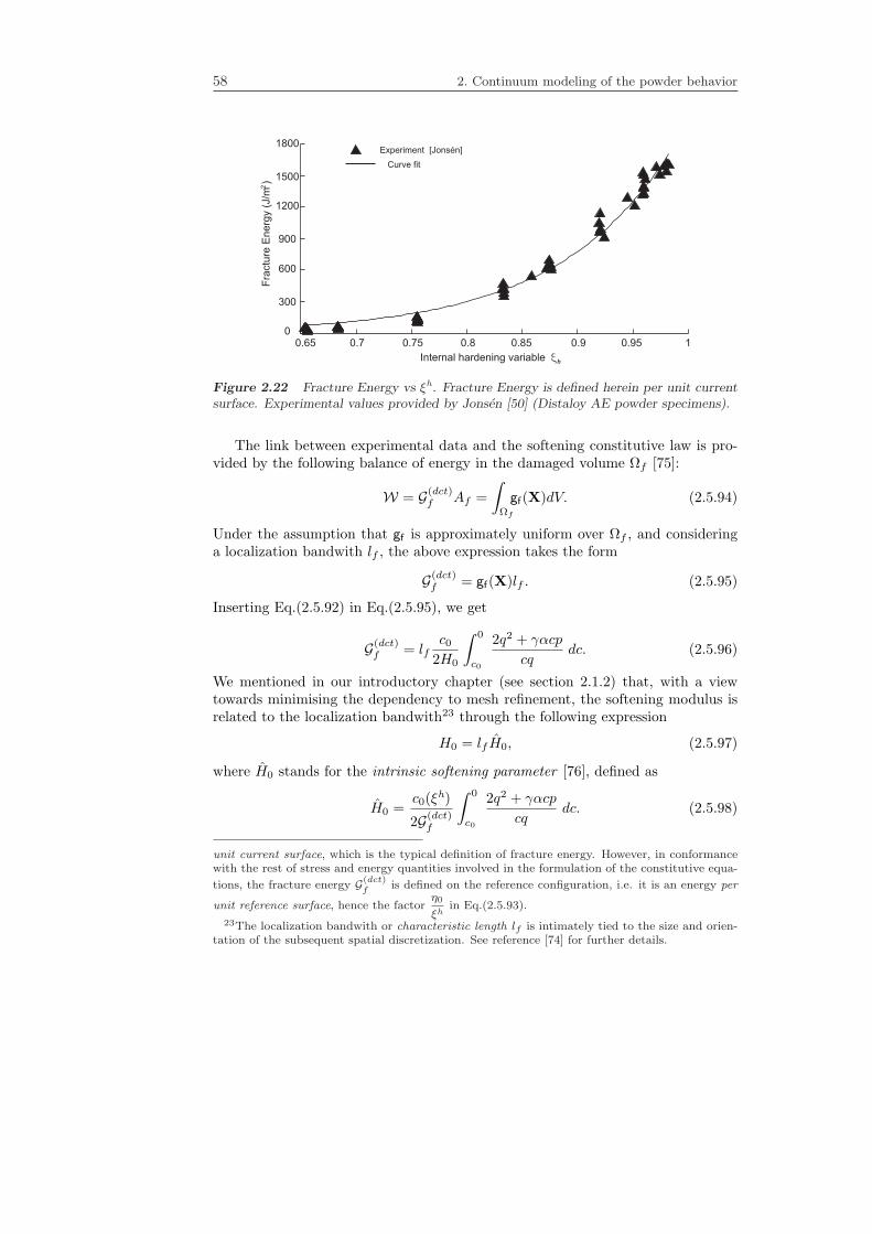
58 2. Continuum modeling of the powder behavior
hxInternal hardening variable
0.65 0.7 0.75 0.8 10.85 0.9 0.950
300
600
900
1200
1500
1800Experiment [Jonsén]
Curve fit
Fra
ctu
re E
nerg
y (
J/m
)2
Figure 2.22 Fracture Energy vs ξh. Fracture Energy is defined herein per unit currentsurface. Experimental values provided by Jonsen [50] (Distaloy AE powder specimens).
The link between experimental data and the softening constitutive law is pro-vided by the following balance of energy in the damaged volume Ωf [75]:
W = G(dct)f Af =
∫
Ωf
gf(X)dV. (2.5.94)
Under the assumption that gf is approximately uniform over Ωf , and consideringa localization bandwith lf , the above expression takes the form
G(dct)f = gf(X)lf . (2.5.95)
Inserting Eq.(2.5.92) in Eq.(2.5.95), we get
G(dct)f = lf
c02H0
∫ 0
c0
2q2 + γαcp
cqdc. (2.5.96)
We mentioned in our introductory chapter (see section 2.1.2) that, with a viewtowards minimising the dependency to mesh refinement, the softening modulus isrelated to the localization bandwith23 through the following expression
H0 = lf H0, (2.5.97)
where H0 stands for the intrinsic softening parameter [76], defined as
H0 =c0(ξh)
2G(dct)f
∫ 0
c0
2q2 + γαcp
cqdc. (2.5.98)
unit current surface, which is the typical definition of fracture energy. However, in conformancewith the rest of stress and energy quantities involved in the formulation of the constitutive equa-
tions, the fracture energy G(dct)f is defined on the reference configuration, i.e. it is an energy per
unit reference surface, hence the factorη0
ξhin Eq.(2.5.93).
23The localization bandwith or characteristic length lf is intimately tied to the size and orien-tation of the subsequent spatial discretization. See reference [74] for further details.

2.5 Plastic response 59
The superindex “dct” attached to the symbol Gf indicates that this quantitycorresponds to the fracture energy measured in a diametral compression test. Theintrinsic softening H0, on the other hand, is not accompanied by any superindex.This notational convention has been deliberately introduced to highlight one ofour basic assumptions in this regard. Indeed, whereas fracture energy is clearlya quantity sensitive to the loading history followed during the experimental test,we shall consider that the intrinsic softening parameter does not depend on theloading history. In other words, we regard the intrinsic softening parameter H0
as a state function, i.e., a quantity that can be uniquely determined at any timeby the point values of the state variables. In this case, according to Eq.(2.5.98)and Eq.(2.5.93), the softening parameter only depends on the internal hardeningvariable, that is H0 = H0(ξh). The intrinsic softening modulus is then defined byanalogy with Eq.(2.5.80) as:
H = H0c0 + csc0
, (2.5.99)
is also a state function, but it further depends on the internal softening variable,H = H(ξh, ξs). Note that neither the softening modulus H nor the softeningparameter H0 can be viewed as state functions.
To complete the calibration, it would be now pertinent to evaluate analyticallythe integral appearing in Eq.(2.5.98). To this end, one needs the analytical expres-sion of the stress path traced during the de-cohesion process at points within thecracking band. For the case of a diametral compression test, the derivation of suchexpressions is far from being obvious, as it may surmised from the stress analysis(in the elastic range) carried out by Timoshenko [102].
To overcome this difficulty, it proves advantageous to exploit the fact that thediametral compression test is but an indirect test to measure the tensile strengthof brittle or quasi-brittle materials (hence the alternative denomination of indirecttension test [107]), on which direct uniaxial tensile test are difficult to perform.The experimental configuration of the diametral compression test is such that thedeveloping of the crack at the loaded diameter takes place under Mode I or openingmode conditions, which, in turn, are the same conditions encountered in a standarduniaxial tensile test. On this basis, a plausible assumption is to consider that thefracture energy measured in a uniaxial tensile test is approximately equal to thatcorresponding to the diametral compression test, i.e.:
G(dct)f ≈ G(tt)
f , (2.5.100)
the superindex “tt” signifying tensile test. Under such assumption, the analyti-cal evaluation of the integral in Eq.(2.5.98) becomes feasible, as we show in thefollowing.
In a uniaxial tensile test, the ratio q/p at points belonging to the cracking bandis approximately linear:
q ≈ m p, (2.5.101)
since necking is not very pronounced in quasi-brittle materials [41] and thus theuniaxial stress state prevails after bifurcation of the response. For a tensile test,

60 2. Continuum modeling of the powder behavior
m =√
6, as it is deduced from figure 2.18.a. Enforcing the yield condition inEq.(2.5.101), we get an expression of q as a function of the cohesion c:
q =m
m + αc = mc. (2.5.102)
Inserting the above equation into Eq.(2.5.98) and integrating, an expression for theintrinsic softening modulus H0 is finally achieved:
H0 = − c20
2G(dct)f
2m2 − γm + γ
m. (2.5.103)
Inspection of the empirical laws (2.5.93) and (2.5.56) shows that both are expo-nential functions of the internal hardening variable. It follows from Eq.(2.5.103),thus, that the dependence of the intrinsic softening parameter on ξh exhibits alsoan exponential format:
|H0(ξh)| = η0ξhAHe
BHξh
, (2.5.104)
where
AH =2(m2 − γm + γ)
3m
A2ch
AGf
, (2.5.105)
BH = 2Bch −BGf. (2.5.106)
In figure 2.23, relation (2.5.104) between the intrinsic softening parameter |H0|and ξh is plotted. The graph shows that H0 is close to zero for the range oflow densities. This observation confirms the hypothesis made in section 2.3, andrepresented by Eq.(2.3.3) , asserting that the softening mechanism is not activefor low densities. Another interesting conclusion can be drawn from the valuesdisplayed in figure 2.23. The magnitude of |H0| for ξh ≈ 0.95 is approximately 1.0MN/mm3. Considering a typical width crack of, say, 0.1 mm, the resulting valueof the softening parameter would be |H0| = 0.1 · 1.0MN/mm2 = 0.1 · 106MPa.On the other hand, the Young’s Modulus corresponding to the same density range(see figure 2.17) is approximatelyEe ≈ 150GPa = 0.15 · 106MPa. This gives aratio Ee/H0 ≈ 1.5, i.e., both moduli are of the same order of magnitude, which,in turn, implies that the order of magnitude of elastic and plastic strains are thesame in deformation processes entailing only softening. This assertion is one of thebasic assumptions made in section 2.2.1.
A noteworthy feature of the present approach is the hypothesis presented aboveby which the intrinsic softening parameter H0 is regarded as a state variable. Thelack of experimental data concerning fracture energy in other fracture tests pre-cludes the possibility of strictly corroborating this hypothesis. Nevertheless, itwould be instructive to briefly examine and put on a quantitative basis the conse-quences of such proviso. For this purpose, consider a compression test characterized

2.5 Plastic response 61
hxInternal hardening variable
0.4 0.5 0.6 0.80.7 0.9 1
0
5
7.5
12.5
10
15
x 105
2.5
Intr
insic
Softenin
g M
odulu
s (
N/m
m )
3
Figure 2.23 Intrinsic softening parameter H0 vs internal hardening variable ξh.
by a stress path during plastic loading given by q = −√6p (see figure 2.14.b) 24. Fora typical value γ = 0.01 of the dilatational coefficient and a parameter of internalfriction α = 2.29, we get
H0 = −15.8c20
2G(ct)f
. (2.5.107)
where G(ct)f stands for the fracture energy associated to a uniaxial compression test.
The same operations for a uniaxial tensile test yields
H0 = −0.52c20
2G(tt)f
. (2.5.108)
In view of Eq.(2.5.107) and Eq.(2.5.108), the fracture energy measured in a uniaxialcompression test would be 15.8/0.52 ≈ 30 times greater that the linked to the oneobtained in a uniaxial tensile test. For other granular media, such as concrete, thisratio gives approximately 100 [82].
24The ratio q/p is not linear in a compression test after bifurcation, since important shearstresses develop at the localization band [61] (fracture occurs under shear mode or mode II con-ditions (see figure 2.6)) and, consequently, the hypothesis of uniaxial stress state is no longervalid. However, the approximation adopted here q/p = −√6 (the same path traced during elasticloading) serves as a first approximation for estimating the fracture energy associated to this test.

62 2. Continuum modeling of the powder behavior

Chapter 3
Integration of theconstitutive equation
3.1 Preliminaries
The preceding chapter was devoted to describe mathematically the effects that agiven deformation history has on the physical attributes of the powder at a pointX ∈ Ω0 . The result was the formulation of a system of constitutive laws andevolution equations subjected to a set of unilateral constraints. For clarity, wesummarize again these relations:
I. Deformation and strain history up to current time t ∈ [t0, tf ] (given):
t 7→ Ft(X) = F(X, t), where t ∈ [t0, t], (3.1.1)
e =12
(1− F-T ·F-1
). (3.1.2)
II. Elastic strain-stress relationship
τ =
τ0︷ ︸︸ ︷F · S0 · FT + ce : (e− ep), where S0 = S(t0), (3.1.3)
ce = κe1⊗ 1 + 2µe(I − 131⊗ 1), (3.1.4)
with κe = κe(ξh) and µe = µe(ξh) given in Eqs. (2.4.2) and (2.5.60).
III. Elastic domain in Kirchhoff stress space
Eτ =τ | φβ(τ , ξh, ξs) ≤ 0, for all β ∈ e, d, v , where (3.1.5)
φe = φ1 = q2 + s22(ξh)p2 − s21(ξh)s22(ξh), (3.1.6)
63

64 3. Integration of the constitutive equation
φd = φ2 = q + αp− c(ξh, ξs), (3.1.7)
φv = φ3 = q − cv(ξh), (3.1.8)
with p = 13 tr τ and q =
√dev τ : dev τ .
IV. Flow rule
Lvep = dp =3∑
β=1
λβmβ , where (3.1.9)
me = m1 = 2dev τ +23s22(ξ
h)p1, (3.1.10)
md = m2 = 2 dev τ +13γ c(ξh, ξs)α1, (3.1.11)
mv = m3 = 2 dev τ . (3.1.12)
V. Evolution of internal variables
ξh = −ξhλe2s22(ξh)p, (3.1.13)
ξs = 2λdq, (3.1.14)
with initial values ξh(t0) = η0 and ξs(t0) = 0.
VI. Softening and hardening laws (in rate form)
s1 =∂s1h∂ξh
ξh, (3.1.15)
s2 =∂s2h∂ξh
ξh, (3.1.16)
c =∂ch∂ξh
ξh +Hξs, (3.1.17)
cv =∂cvh∂ξh
, (3.1.18)
where s1h = s1h(ξh), s2h = s2h(ξh), ch = ch(ξh), H = H(ξs) and cvh =cvh(ξh) are given in Eqs. (2.5.53), (2.5.54), (2.5.56), (2.5.80) and Eq.(2.5.59),respectively.
VII. Karush-Kuhn-Tucker loading/unloading conditions and consistency condition
λβ ≥ 0, φβ(τ , ξh, ξs) ≤ 0, (3.1.19)
λβφβ(τ , ξh, ξs) = 0, (no sum on β), (3.1.20)
λβφβ(τ , ξh, ξs) = 0, (no sum on β). (3.1.21)

3.1 Preliminaries 65
The underlying ODE structure of the governing equations listed above becomesapparent by expressing all the variables involved in the problem in terms of aset of generalized stresses, defined as Σ = (S, r), where S is the second Piola-Kirchhoff stress tensor and r stands for the stress-like vector of internal variablewith components:
r =[s1c
], (3.1.22)
which, in turn, is related with the vector of strain-like internal variables [ξh, ξs]T
through the generalized plastic moduli D, defined as
D =
∂s1h∂ξh
0
∂ch∂ξh
H
. (3.1.23)
By performing pull-back transformations on the constitutive equations, and aftersome straightforward, albeit lengthy, manipulation, one gets the following general-ized representation of the system of ordinary differential equations governing thelocal response of the powder at X ∈ Ω0
1:
Σ = A(Σ, E) +3∑
β=1
λβΞβ(Σ). (3.1.24)
This system is supplemented with the initial conditions Σ(t0) = (S0, r(ξ0)). Thecomponents of the generalized stress tensor Σ and the plastic multipliers λβ , (β =1, 2, 3) are the dependent variables, whereas the rate of change of the Green-Lagrange strain tensor E is the source term. The evolution of Σ is further re-stricted by the loading/unloading and consistency conditions, which in terms of Σare written as
λβ ≥ 0, φβ(Σ) ≤ 0, (3.1.25)
λβφβ(Σ) = 0, (no sum on β), (3.1.26)
λβφβ(Σ) = 0, (no sum on β). (3.1.27)
The problem of integrating numerically the initial-value ODE equation repre-sented by Eq.(3.1.24), in conjunction with conditions (3.1.25), (3.1.26) and (3.1.27),constitutes the central problem of computational plasticity [92]. The remainder ofthis chapter is focused on solving this problem and addressing the mathematicalquestions that arises in its treatment.
1The derivation of the expressions for A = A(Σ, E) and Ξβ = Ξβ(Σ) is not quoted herein.The interested reader is urged to consult Appendix A.2 for the details of such derivation.
66 3. Integration of the constitutive equation
3.1.1 Implicit Backward-Euler and IMPLEX integrationschemes
As customarily, the continuous time domain [t0, tf ] of interest is discretized innon-overlapping intervals, [t0, tf ] =
⋃Nn=1[tn, tn+1]. Then, the exact derivative in
Eq.(3.1.24) is approximated by an algebraic finite difference. Finally, substitutionof this approximation into the ODE equation leads to an algebraic finite differenceequation [45]. One of the most employed methods in computational plasticity ariseswhen the derivative at time tn+1 is approximated as
(Σ
)n+1≈ Σn+1 −Σn
∆tn+1. (3.1.28)
The resulting finite difference scheme is known as the implicit Backward Eulerdifference scheme. The associated non-linear difference equation takes the form
Σn+1 −Σn = ∆tn+1A(Σn+1, En+1) +∑
β∈Jact
∆λβn+1 Ξβ(Σn+1), (3.1.29)
where ∆tn+1 = tn+1 − tn and ∆λβn+1 = ∆tn+1λβ stand for the length of the
time interval and the β-th discrete plastic multiplier, respectively. The discretecounterpart of the Karush-Kuhn-Tucker conditions (3.1.25), (3.1.26) and (3.1.27)read
∆λβn+1 ≥ 0, φβ(Σn+1) ≤ 0, (3.1.30)
∆λβn+1φβ(Σn+1) = 0, (no sum on β). (3.1.31)
The reason behind the popularity of such method is, on one hand, that itprovides a suitable framework for the enforcement of the algebraic Karush-Kuhn-Tucker constraints, leading to the classical return mapping algorithm [92]. On theother hand, the implicit Backward Euler scheme turns out to be, in general, uncon-ditionally stable [93]. Section 3.2 is devoted to discuss the salient features of suchintegration scheme when applied to our specific problem. One of the issue that willreceive particular consideration is that of the uniqueness of solution. As a matterof fact, the task of ensuring the existence and uniqueness of solution will requireto modify the evolution equations (3.1.13) and (3.1.14), although these modifica-tions will be accommodated without significantly compromising the adequacy ofthe empirical correlations established in the previous chapter.
The source term in the ODE (3.1.24) is the rate of change of the Green-Lagrangestrain tensor E. This fact is consistent with the strain-driven character of the con-stitutive model, whereby all variables can be expressed in terms of the deformationhistory through adequate functional relationships. Therefore, the deformation his-tory is presumed known when solving the ODE (A.2.13). From the algorithmicpoint of view, this statement means that the strain rate is prescribed in the inter-val [tn, tn+1] when solving the associated difference equation (3.1.29).
In practice, however, the function F = F(t), t ∈ [t0, tF ] is not available as such.Our aim is to obtain the mechanical response of the powder sub-system under

3.1 Preliminaries 67
external loads (punch actions). To this end the weak form of the momentum equa-tion is discretized via a Galerkin finite element projection2. Then, the numericalsolution of the discrete system of equations, whose basic unknowns are the nodaldisplacements, is obtained by performing an incremental analysis accompanied byiterations so as to ensure convergence to equilibrium states. The strain increment∆E = En+1−En is calculated from the current displacement field, which is updatedat the beginning of each iteration, and the previously converged configuration (attn) through adequate kinematic relationships.
If a standard Newton-Raphson procedure is employed for this iterative pro-cess, as is the case here, the spectral properties of the so-called algorithmic tangentmoduli are a crucial issue for preserving the quadratic rate of asymptotic conver-gence that characterizes Newtown’s method. It is widely known that if the posi-tive definiteness of the the algorithmic tangent moduli cannot be guaranteed, theperformance of the Newton-Raphson method may be seriously impaired, affectingeventually the ability of the considered algorithm to provide results at affordablecomputational costs. The algorithmic tangent moduli stemming from the implicitintegration of an elasto-plastic model equipped with softening, as in our case, is atypical example in which the proviso of positive definiteness is not satisfied, a factintimately tied with the character of unstable material model associated to thistype of approach [6].
The need to circumvent this barrier to computability has prompted investi-gations of alternative means of integrating the constitutive model. The solutionadopted herein is the one pioneered by Oliver et al. [79, 80], originally conceivedfor addressing the problem of robustness and stability arising in the numericalsimulation of material failure within the framework of the Strong DiscontinuityApproach. The algorithmic details concerning this integration scheme are given insection 3.3.
Oliver et al. coined the term IMPLEX (IMPLicit-EXplicit) to suggest thatthe proposed methodology shares some of the features of both implicit and ex-plicit integration schemes. The essence of the method is to solve explicitly forsome variables, in the sense that the values at the beginning of the increment arepresumed known, and implicitly for other group of variables. In this aspect, theIMPLEX methodology parallels that followed in the so-called semi-implicit integra-tion scheme, developed by Moran et al. [68, 5]3. However, the primary motivationbehind the semi-implicit strategy is to reduce the equation solving effort associatedto the solution of the fully implicit scheme, whereas the IMPLEX method is basi-cally intended to enhance the spectral properties of the algorithmic tangent moduli.Indeed, the remarkable stability exhibited by IMPLEX solutions [80] is attributedto the fact that the above mentioned group of explicit variables are extrapolatedvalues of the same quantities computed at previous time steps by accomplishing afully implicit integration. The distinguishing feature of the IMPLEX methodologyis, hence, that it does entail the solution at each time increment of the non-linear
2So far, attention has been confined to the local response at a point X ∈ Ω0, which, in fact,corresponds to a quadrature point of a typical finite element
3This integration procedure is characterized for being implicit in the incremental plastic strain,but explicit in the plastic flow direction and the hardening moduli

68 3. Integration of the constitutive equation
system of equations stemming from the implicit backward-Euler difference scheme.Furthermore, with an appropriate choice of the explicit variables, the algorith-
mic tangent tensor adopts a very simplified format, to such an extent that if theterms due to non-linear kinematics are discarded, the resulting tangent tensor isstep-constant. This means that if one disregards other sources of non-linearitiesrather than the material one, the structural tangent stiffness matrix would be con-stant and the convergence to equilibrium states could be achieved, theoretically,in only one iteration per time step, as it is shown in the original work of Oliveret al.[79]. A further implication of this statement is that, if during a computerrun the convergence of the global Newton-Raphson iteration scheme is hinderedby any reason, one should seek the causes that inhibit convergence in geometricsingularities or in the roughness of the response associated to the contact with thepunches (boundary conditions) rather than in material non-linearities.
Although the IMPLEX integration, as the fully implicit scheme, is first-orderaccurate [80], the global error associated to the IMPLEX scheme is comparativelylarger for the same time step size. Hence, the IMPLEX method demands moretime steps than the implicit procedure for obtaining the same accuracy in theresults. Nevertheless, the consequences of this drawback are not too drastic, since,in practical loading situations, the step size is to be considerably reduced by theneed to accurately resolve the abrupt nature of the contact response between thepowder and the tooling.
Another characteristic of this integration scheme is that the yield condition isnot enforced at time tn+1, i.e, the updated stresses emanating from the IMPLEXintegration violates the consistency condition. Note that this is a feature inherentto the explicit character of the proposed method. It should be remarked, however,that in contrast to standard explicit forward Euler procedures [27], the accumu-lated error remains bounded as the solution progresses[80]. Indeed, if one considersa process involving yielding in which the application of the external actions arereasonably smooth, the explicit values, obtained as extrapolations of implicitly in-tegrated quantities at previous steps, would not differ substantially from thosefurnished by a fully implicit scheme at time tn+1, and thus the stress state wouldremain very close to the boundary of the elastic domain. By contrast, in thosecircumstances in which the response is far from being smooth, as in the abrupttransition from compressive yielding to elastic conditions that accompanies the up-per punch pressure release, the yield condition may be substantially violated. Inorder to overcome this adverse effect, Oliver et al.[80] have proposed an adaptivetime step algorithm that keeps the error in these cases into appropriate bounds.
3.2 Implicit integration scheme
We consider a time discretization of the interval [t0, tf ] =⋃Nn=1[tn, tn+1], and let
ξhn, ξsn,En,Ep,n be the initial data at tn. We regard also the deformation gradientFn+1 at tn+1 as given. Our aim is to find the state variables at the end of theinterval [tn, tn+1] by applying a implicit backward Euler difference scheme to theconstitutive evolution equations summarized at the beginning of this chapter.

3.2 Implicit integration scheme 69
We begin by the elastic constitutive relationship (3.1.3). Since this relation isnot expressed in rate form, we can simply write its discrete counterpart as:
τn+1 = Fn+1 · S0 · FTn+1 + ce,n+1 : (en+1 − ep,n+1). (3.2.1)
Observe that the notation ce,n+1 indicates that ce,n+1 = ce(ξhn+1). In order tosatisfy the requirement of objectivity, the flow rule represented by Eq.(3.1.9) istransformed back to the reference configuration Ω0 and then approximated as:
Ep,n+1 = Ep,n +3∑
β=1
∆λβn+1ϕ∗(mβn+1
), (3.2.2)
where ∆λβn+1 denotes the discrete plastic multiplier ∆λβn+1 = ∆tn+1 λβ , with
∆tn+1 = tn+1 − tn. The symbol ϕ∗(•) stands for the pull back operator4 ϕ∗(•) =F-Tn+1 · (•) ·F-1
n+1. We revert again to the spatial description by obtaining the pushforward, defined as ϕ∗(•) = F-T
n+1 · (•) · F-1n+1, of Eq.(3.2.2):
ϕ∗(Ep,n+1) = ϕ∗(Ep,n) +∑
β∈Jact
∆λβn+1ϕ∗(ϕ∗
(mβn+1
))⇒
ep,n+1 = ep,n +∑
β∈Jact
∆λβn+1mβn+1. (3.2.3)
Remark 3.2.1. The breve symbol in ep,n is attached to indicate that ep,n is a strainmeasure computed at time tn but transformed to the current configuration Ωn+1
via a push forward operation:
ep,n = ϕ∗(Ep,n) = F-Tn+1 ·Ep,n · F-1
n+1. (3.2.4)
The above can be rephrased also, after simple algebra, in terms of the incrementaldeformation gradient ∆Fn+1 = Fn+1 · F-1
n ,
ep,n = F-Tn+1 ·Ep,n · F-1
n+1 = ∆F-Tn+1 · ep,n ·∆F-1
n+1, (3.2.5)
or symbolically,ep,n = ϕ∆
∗ (ep,n) , (3.2.6)
ϕ∆∗ (•) being the push-forward operation relating the incremental motion from con-
figuration Ωn to Ωn+1. This notation will be used henceforth to denote any tensorialquantity computed at tn but pushed forwardly to the current configuration Ωn+1.In this way, for instance, τn = ϕ∗(Sn) = ϕ∆
∗ (τn). This notational convention willpermit us to easily draw analogies with infinitesimal classical plasticity formula-tions, by simply setting ep,n ≈ ep,n, or τn ≈ τn = σn.
4Push-forward and pull-back transformations depend on the covariant or contra-variant na-ture of their arguments. Strain measures are considered herein covariant tensors, whereas stressquantities are contravariants. For further details, see Appendix A, Eqs. (A.1.12) and (A.1.13)

70 3. Integration of the constitutive equation
The same approximation of the time derivative is carried out on the evolutionequations (3.1.13) and (3.1.14), leading to the following difference equations:
ξhn+1 = ξhn − 2ξhn+1∆λen+1s2,n+1
2 pn+1, (3.2.7)
ξsn+1 = ξsn + 2∆λdn+1qn+1, (3.2.8)
where pn+1 = 1/3tr τn+1 and qn+1 = ‖dev τn+1‖. The parameters governing thesize and shape of the elliptical cap surface and the location of Von Mises yieldsurface can be obtained through functional evaluations, i.e. s1,n+1 = s1(ξhn+1),s2,n+1 = s2(ξhn+1) and cv,n+1 = cv(ξhn+1). On the other hand, the expression forthe cohesion state variable can be drawn from the rate equation (3.1.17) as:
cn+1 = cn +∂ch∂ξh
∣∣∣∣n+1
(ξhn+1 − ξhn) +Hn+1(ξsn+1 − ξsn). (3.2.9)
Finally, the discrete counterpart of the Karush-Kuhn-Tucker loading/unloadingconditions are given by
∆λβn+1 ≥ 0, φβn+1 ≤ 0, (β = 1, 2, 3) (3.2.10)
∆λβn+1φβn+1 = 0, (β = 1, 2, 3) (no sum on β). (3.2.11)
whereφen+1 = φ1
n+1 = q2n+1 + s2,n+12 p2
n+1 − s1,n+12 s2,n+1
2, (3.2.12)
φdn+1 = φ2n+1 = qn+1 + αpn+1 − cn+1, (3.2.13)
φvn+1 = φ3n+1 = qn+1 − cv,n+1. (3.2.14)
A widely used procedure, which can be justified as a product formula based onan elastic-plastic operator split [92], to cast the loading-unloading conditions in aformat readily amenable to computational implementation is to introduce the trialelastic state. This trial state arises from assuming elastic behavior throughout thetime step [tn, tn+1]:
etrp,n+1 = ep,n, (3.2.15)
ξh,trn+1 = ξhn, (3.2.16)
ξs,trn+1 = ξsn. (3.2.17)
τ trn+1 = Fn+1 · S0 · FTn+1 + ce,n : (en+1 − ep,n). (3.2.18)
If the convexity of the elastic domain holds5, it can be shown [92] that if
φβ,trn+1 = φβ(τ trn+1, ξh,trn+1, ξ
s,trn+1) < 0, ∀β = 1, 2, 3, (3.2.19)
5By examination of figure 2.7 (section 2.5.2), and by straightforward geometric considerations,we can immediately conclude that the elastic domains displayed are convex in stress space. For atypical Distaloy AE, whose empirical correlations were detailed in section 2.5, this conclusion canbe extended for the whole range of possible configurations of the three yield surfaces. For othermaterials, the fulfillment of the convexity condition must be inspected cautiously.

3.2 Implicit integration scheme 71
then the trial elastic state is inside the elastic domain and, therefore, the deforma-tion is entirely elastic. In this case, the updated state corresponds to the aboveshown trial elastic state. By contrast, if one or more yield conditions are violated,i.e.
φβ,trn+1 > 0, for any β = 1, 2, 3, (3.2.20)
then the tentative assumption of elastic response is rejected, and the updated stateis obtained by “returning” the trial state to the yield surface, in order to meet thecorresponding consistency condition.
The computation of elastic predictor step does not entail any difficulty, sinceit involves only functional evaluations. The complexity lies thus in the plasticcorrector step, which constitutes the thrust of the return mapping algorithm. Acrucial issue in return mapping algorithms with multisurface yield conditions is thedetermination of the set of active constrains [92], defined as
Jactn+1 =β ∈ 1, 2, 3 | ∆λβn+1 > 0
. (3.2.21)
One salient feature of this set of active constrains is that Jactn+1 ⊆ Jact,trn+1 , whereJact,trn+1 is given by
Jact,trn+1 =β ∈ 1, 2, 3 | φβ,trn+1 > 0
. (3.2.22)
This assertion means that if only one yield condition φα,trn+1 is violated, then ∆λαn+1 >
0, but if several yield conditions are active, then the condition φα,trn+1 > 0 does notguarantee that ∆λαn+1 > 0 [92].
Inserting the discrete flow rule (3.2.2) in Eq.(3.2.1), we get
τn+1 =Fn+1 · S0 · FTn+1 + ce,n+1 : (en+1 − ep,n)
−3∑
β=1
∆λβn+1 ce,n+1 : mβn+1.
(3.2.23)
Using the preceding relation and the definition (3.2.18) of trial stress, an easymanipulation produces the result
τn+1 = τ trn+1 + ∆ce,n+1 : (en+1 − ep,n)−3∑
β=1
∆λβn+1 ce,n+1 : mβn+1. (3.2.24)
The fourth-order tensor ∆ce,n+1 in the above expression, defined as
∆ce,n+1 = ce(ξhn+1)− ce(ξhn) = (κen+1 − κen)1⊗ 1 + 2 (µen+1 − µen)Idev. (3.2.25)
does not appear in classical plasticity formulation. This term reveals the couplingbetween elastic and plastic responses, i.e. the fact that the elastic moduli Ee
increases as hardening progresses.
Remark 3.2.2. Expression (3.2.24) possesses a compelling geometric interpretation,illustrated in figure 3.1. The projection of the trial elastic stress τ trn+1 in the p-q

72 3. Integration of the constitutive equation
q
p
1n
tr
+τ
D
( )1n+Dc
1n+e
n
pe(
: -
1n
el
+D
em
1n+c :
1
1
ns
+-
1n+τ
1n
el
+D
em
1n+c :
1
ns-
Figure 3.1 Geometrical interpretation of the effect of coupling between elastic andplastic response.
plane lies outside the elastic domain. Since only the elliptical yield surface is active,then ∆λen+1 > 0 and ∆λdn+1 = ∆λvn+1 = 0. The unusual feature here is thatthe return direction is not determined by the vector ce,n+1 : me
n+1. Rather, thelocation of the trial stress is changed to τ trn+1 +∆ce,n+1 : (en+1− ep,n) before beingprojected back to the yield surface using the direction ce,n+1 : me
n+1. Anotherremarkable feature is that, as the Poisson’s ratio is regarded as a constant, thedirection determined by ∆ce,n+1 : (en+1 − ep,n) is aligned with ce,n+1 : (en+1 −ep,n).
Therefore, the effect of the coupling between plastic and elastic response isthe alteration of the projection direction. In Appendix A.2, remark A.2.1, it is
concluded that the altered plastic flow vector4me, defined from the following ex-
pression
∆λen+1 ce,n+1 :
4me = ∆λe
n+1 ce,n+1 : men+1 −∆ce,n+1 : (en+1 − ep,n), (3.2.26)
differs from the associated flow vector men+1 by terms that are one order of mag-
nitude larger than the elastic strains.
For convenience, we summarize in BOX 3.2 the resulting nonlinear coupledsystem for the unknown state variables at tn+1.
3.2.1 Modification of the evolution equations
Our attention is concentrated now on the system of non-linear equations listedin BOX 3.2. The presence of the unilateral constrain, represented by the loading-unloading conditions, renders the task of solving this system of equations a challeng-ing task. A widely employed strategy [92] for tackling such problem is to interpret
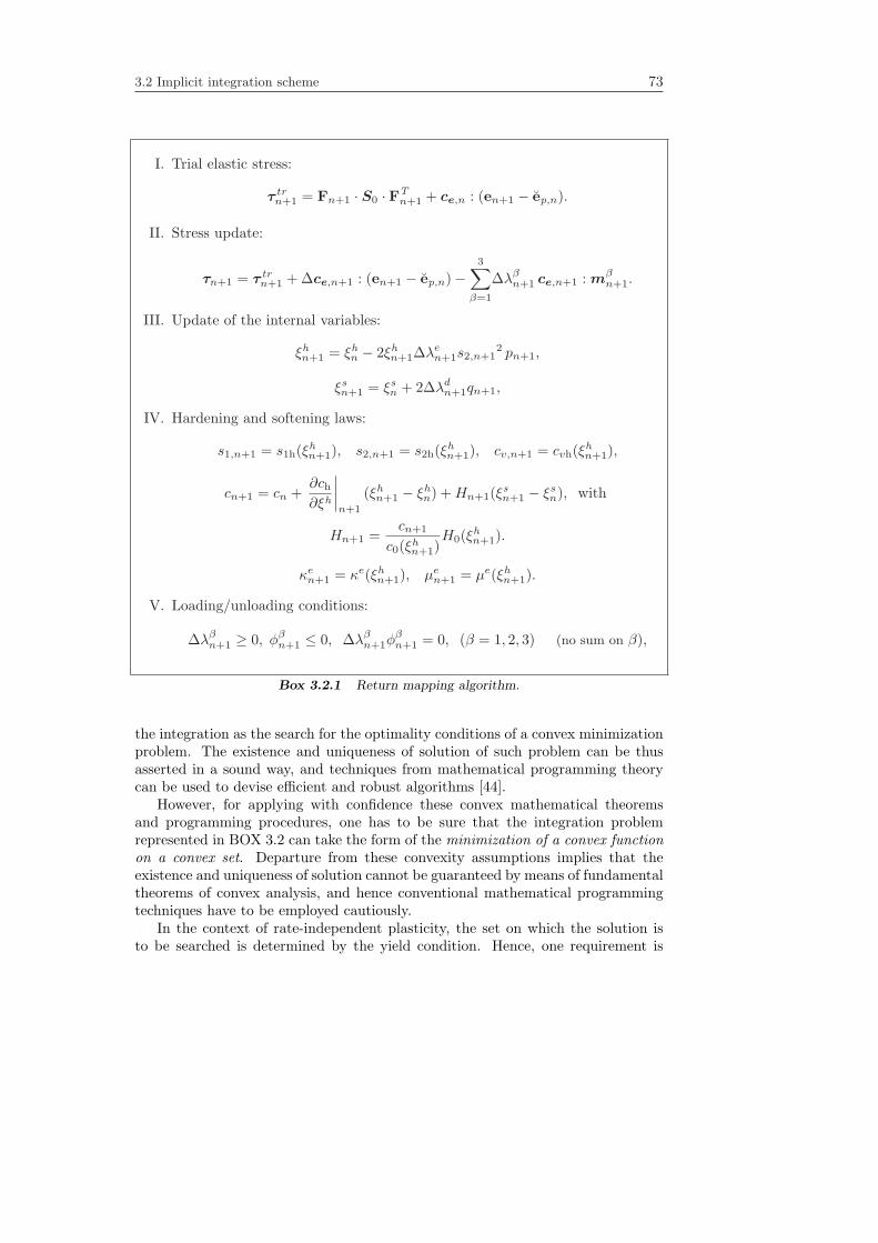
3.2 Implicit integration scheme 73
I. Trial elastic stress:
τ trn+1 = Fn+1 · S0 · FTn+1 + ce,n : (en+1 − ep,n).
II. Stress update:
τn+1 = τ trn+1 + ∆ce,n+1 : (en+1 − ep,n)−3∑
β=1
∆λβn+1 ce,n+1 : mβn+1.
III. Update of the internal variables:
ξhn+1 = ξhn − 2ξhn+1∆λen+1s2,n+1
2 pn+1,
ξsn+1 = ξsn + 2∆λdn+1qn+1,
IV. Hardening and softening laws:
s1,n+1 = s1h(ξhn+1), s2,n+1 = s2h(ξhn+1), cv,n+1 = cvh(ξhn+1),
cn+1 = cn +∂ch∂ξh
∣∣∣∣n+1
(ξhn+1 − ξhn) +Hn+1(ξsn+1 − ξsn), with
Hn+1 =cn+1
c0(ξhn+1)H0(ξhn+1).
κen+1 = κe(ξhn+1), µen+1 = µe(ξhn+1).
V. Loading/unloading conditions:
∆λβn+1 ≥ 0, φβn+1 ≤ 0, ∆λβn+1φβn+1 = 0, (β = 1, 2, 3) (no sum on β),
Box 3.2.1 Return mapping algorithm.
the integration as the search for the optimality conditions of a convex minimizationproblem. The existence and uniqueness of solution of such problem can be thusasserted in a sound way, and techniques from mathematical programming theorycan be used to devise efficient and robust algorithms [44].
However, for applying with confidence these convex mathematical theoremsand programming procedures, one has to be sure that the integration problemrepresented in BOX 3.2 can take the form of the minimization of a convex functionon a convex set. Departure from these convexity assumptions implies that theexistence and uniqueness of solution cannot be guaranteed by means of fundamentaltheorems of convex analysis, and hence conventional mathematical programmingtechniques have to be employed cautiously.
In the context of rate-independent plasticity, the set on which the solution isto be searched is determined by the yield condition. Hence, one requirement is

74 3. Integration of the constitutive equation
the convexity of the elastic domain in the space of generalized stresses. The otherstandard prerequisite is that the diagonal compliance operator
G =[ce−1 00 D−1
], (3.2.27)
is to be positive definite, so as to ensure that it defines a metric, i.e. Σ : G : Σ ≥ 0for all Σ. Clearly, this is not the case, since the generalized hardening moduli D(see Eq.(3.1.23)) lacks positiveness when the softening mechanism is active (H < 0).Hence, we see that, again, the presence of softening affects adversely the algorithmictreatment of our model by means of standard procedures.
In view of these circumstances, we are compelled to find other means to bothensure the existence and uniqueness of solution and devise an algorithm to effi-ciently find this solution. As it may be surmised, this is not an obvious task, due tothe tightly coupled character of the governing equations. The two main sources ofdifficulties are the coupling between elastic and hardening behavior, symboliced bythe term ∆ce,n+1 : (en+1 − ep,n) in Eq.(3.2.24), and the coupling between harden-ing and softening, which takes place when the return mapping algorithm places theupdated stresses on the intersection between the Drucker-Prager and the ellipticalyield surfaces. The following two items explained how to alleviate these difficultiesby modifying the evolution equation for the internal variables without eliminatingimportant details of the response.
3.2.1.1 Internal hardening variable
One of the basic assumptions of the proposed model is that the magnitude of theelastic strains is negligible in comparison with the irrecoverable deformations. Aconsequence of such proviso (see section 2.5.1) is that, in the course of monotonicincreasing compressive loading history, the internal variable ξh can be practicallyidentified with the relative density η. In appendix B.2, the validity of this hypothesisis assessed by undertaking an analysis of the monotonic hydrostatic compression ofa cylindrical specimen. The conclusion drawn from this analysis is that the ratiobetween the relative density and internal hardening variable is bounded by
η
ξh≤ e
s1κe . (3.2.28)
Hence, the validity of this assumption hinges on the ratio between the hydrostaticyield stress in compression s1 and the elastic bulk modulus κe. The relation |1 −es1/κ
e | versus η is plotted in figure 3.2 using the empirical correlations derived forthe Distaloy AE powder (see section 2.5.4, Eqs. (2.5.53) and (2.5.60)). It is clearfrom that figure that the difference between relative density and internal hardeningvariable is negligible (∼ 10−3) for almost the whole range of densities. Thereforethe experimentally calibrated values of κe and s1 for a typical Distaloy AE supportthe hypothesis that ξh ≈ η in monotonic increasing compressive loading history.
The only objection that can be raised against this hypothesis is when the relativedensity approaches unity. According to arguments set out in section 2.5.4, the

3.2 Implicit integration scheme 75
hydrostatic yield strength in compression asymptotes to infinity in this event, andsince κe remains bounded, the hypothesis of ξh ≈ η would no longer hold. However,note that in this case neither the kinematics assumptions regarding the additivedecomposition of d and e are valid, and, thus, the usefulness of the numericalprediction as a whole might be questionable. .
0.4 0.5 0.6 0.7 0.8 0.9 1
Relative density -
x 10-3
h
0
1
2
3
4
1-e
1e
s/k
||
Figure 3.2 Function |1− es1/κe | vs η for a typical Distaloy AE powder.
The following proposition demonstrates that the hypothesis of small elasticstrains can be exploit further to derive an approximation of the discrete evolutionequation (3.2.7) for the internal hardening variable.
Proposition 3.2.1. Under the assumption of small elastic deformations, an ap-proximation for the update of the internal hardening variable is given by
ξhn+1 = ξhnHJ (∆λen+1(ηn+1 − ηn), ηnηn+1
)ηn+1
ηn, (3.2.29)
where HJ(•) is the function defined by:
HJ(x, y) =
1, x > 0,y, x ≤ 0, (3.2.30)
and ηn+1 =η0
detFn+1and ηn =
η0detFn
denote the relative densities at time tn+1
and tn, respectively.
Proof.The proof follows easily from the conservation of mass equation and the as-
sumption of negligible elastic strains.¤
The foregoing result admits also an interpretation in the p-q plane. The follow-ing proposition is useful in this regard.

76 3. Integration of the constitutive equation
Proposition 3.2.2. The trial stress defined in Eq.(3.2.18) can be alternativelyexpressed as:
τ trn+1 =¦τn + ∆tn+1 ce,n : dn+1, (3.2.31)
where¦τn is defined through the following formula:
¦τn = τn − (ce,n − ce,n) : (en+1 − ep,n), (3.2.32)
where τn = ϕ∆∗ (τn) and ce,n = ϕ∆
∗ (ce,n).
Proof. First, the constitutive equation at time tn is transformed to configurationΩn+1 via the incremental push forward operator ϕ∆
∗ (•)6, i.e.:
ϕ∆∗ (τn) = ϕ∗(S0) + ϕ∆
∗ (ce,n) : ϕ∆∗ (en+1 − en) . (3.2.33)
This result is subtracted from Eq.(3.2.18), and upon rearrangement, we get
τ trn+1 = ϕ∆∗ (τn)− (ϕ∆
∗ (ce,n)− ce,n) : ϕ∆∗ (en − ep,n) + ce,n : (en+1 − ϕ∆
∗ (en))
= τn − (ce,n − ce,n) : (en+1 − ep,n) + ce,n : (en+1 − ϕ∆∗ (en)).
(3.2.34)
Using the properties of the push forward operator, the last term on the right-handside of the above equation can be written as:
ce,n : (en+1 − ϕ∆∗ (en)) = ce,n : ϕ∗(En+1 −En) . (3.2.35)
Finally, the discrete version of the rate of deformation tensor, which is given by
dn+1 = ϕ∗(E
)≈ 1
∆tn+1ϕ∗(En+1 −En) , (3.2.36)
is substituted into Eq.(3.2.34), yielding the desired result. ¤This alternative format for the trial elastic stress is particularly appealing be-
cause it can be related to the modified evolution equation (3.2.29). Indeed, obtain-ing the volumetric part of Eq.(3.2.31):
ptrn+1 = pn + ∆tn+1 κen trdn+1. (3.2.37)
Using the spatial version of the conservation of mass equation, the above equationcan be expressed as
ptrn+1 = pn + κen logηnηn+1
. (3.2.38)
In virtue of the preceding equation, it turns out that a compressive deformation(ηn+1 > ηn) is characterized by a component of τ trn+1 −
¦τn along the p-axis of the
vector negative, i.e.ptrn+1 ≥ pn ⇒ ηn ≥ ηn+1. (3.2.39)
6The push forward of the double the contraction between a fourth-order tensor and second-order tensor is equal to the double contraction of the push forward of both tensors, i.e. ϕ∗(ce : e) =ϕ∗(ce) : ϕ∗(e).

3.2 Implicit integration scheme 77
It proves expedient to use this result for interpreting graphically the evolutionequation (3.2.29). In figure 3.3, several plausible trial stress states are plotted(labelled from A to F). Only in the situation7 A the internal hardening variableevolves, since the elliptical yield surface is clearly active (∆λen+1 > 0), and thedeformation is compressive ptrn+1 < pn. In the situation encountered in B, notethat ∆λen+1 > 0, but ptrn+1 > pn, hence ξhn+1 = ξhn. The other scenarios, C, Dand E, represent also states in which the internal variable remains in its convergedvalue ξhn.
q
p 1
n
s-
1n
tr
+
τ
1n
tr
+
τ
1n
tr
+
τ
1n
tr
+
τ
1n
tr
+
τ
n
τ
n
τn
τ
n
τ
n
τ
A
B
C
E
D
1p pn n
tr
+- 0<
Figure 3.3 Different scenarios for the evolution of the internal hardening variable. Only
in situation labelled as A, the internal hardening evolves, i.e. ξhn+1 > ξh
n.
3.2.1.2 Internal softening variable
The experimental correlations set forth in sections 2.5.4 and 2.5.5 were obtainedby monitoring the evolution of the corresponding yield stress, say the cohesion c,as one of the internal variables increases, say ξh, and whilst the other (ξs) is heldfixed. Thus, the hardening response is calibrated assuming that no degradationof mechanical strength -softening- occurs during the experiment, and vice versa,softening mechanism is calibrated presuming that ξh does not evolve.
The hardening behavior is linked to yielding on the elliptical cap surface throughthe plastic multiplier λe, and strain softening is associated to yielding on theDrucker-Prager surface through λd. In accordance to Koiter’s rule, when the up-dated stress lies on the intersection ∂Ed,eτ between both yield surfaces, the consis-tency parameters λd and λe are nonzero and, therefore, the hardening and softening
7For illustration purposes,¦τn in situation A have been considered consistent with the yield
condition, i.e φe(¦τn, ξhn) = 0. However, observe that this condition is not necessarily satisfied,
since¦τn 6= τn (only in small strains
¦τn = τn holds).

78 3. Integration of the constitutive equation
mechanism act concurrently. From the physical standpoint, this implies that hard-ening and softening counteract each other, that is, the strain hardening producedby densification is partially counterbalanced by the softening mechanism. Whichof these effects dominates the response eventually cannot be known a priori.
From an algorithmic point of view, this simultaneous occurrence of both hard-ening and softening may cause problems of convergence during the iterations of thereturn mapping algorithm. It is the author’s experience that under such circum-stances the iterates move on and off the active constraints and cause the algorithmto zigzag, placing in each iteration the solution on a different location withoutconverging to any value.
Besides, in a fully implicit integration scheme, inconsistencies during the localintegration of the constitutive equations at any point of the body generally manifestthemselves in other stages of the computational cycle, affecting, for instance, theconvergence of the global iterations. By contrast, in our algorithmic treatment, theinternal forces at tn+1 are computed using stresses stemming from the IMPLEXintegration scheme, and the updated values arising from the implicit integrationare used only, via extrapolation, in subsequent time steps. Consequently, theconvergence of the global iteration scheme may mask the lack of convergence of thelocal iterative procedure associated to the implicit integration, giving a false senseof security by suggesting that everything is correct, while in fact the computedresults may be utterly misleading.
These computational drawbacks motivate the following simplification of thediscrete evolution equation (3.2.8) for the internal softening variable:
ξsn+1 = ξsn +(1−H(∆λen+1)
)(1−H(∆λvn+1)
)2∆λdn+1qn+1. (3.2.40)
where H(•) stands for the Heaviside function. This modification implies that theoccurrence of strain softening is precluded when the updated stress lies on either∂Ed,eτ or ∂Ed,vτ , i.e., the interception points of the Drucker-Prager surface withthe cap surface and with the Von-Mises surface, respectively. It is emphasizedagain that, according to the arguments given in the beginning paragraph, thereare no empirical laws accounting for the simultaneous occurrence of hardening andsoftening an, thus, this modification does not actually compromise the correctnessof the hardening and softening laws derived in sections 2.5.4 and 2.5.5.
3.2.2 Return mapping algorithm using a fractional-step basedmethod.
In this section, the procedure to solve the return-mapping equations is described.The distinguishing feature of this procedure is the iterative process adopted to “re-turn” the trial stress to the yield surface, which is not a standard Newton-Raphsonscheme or variants thereof. The algorithmic procedure is summarized in BOX 3.2.2.
The proposed methodology can be viewed as a natural extension of the two-stepalgorithm derived from the elastic-plastic operator split, in the sense that it consistsin the repetitive application of a predictor-corrector procedure. In each iteration, thepredictor state arises from freezing the internal variables and solving the resulting

3.2 Implicit integration scheme 79
1. Compute trial elastic stress
τ trn+1 = Fn+1 · S0 · FTn+1 + ce,n : (en+1 − ep,n), (3.2.41)
Jact,trn+1 =β ∈ e, d, v | φβ,trn+1 > 0
. (3.2.42)
IF Jact,trn+1 = ∅ THENSet (•)n+1 = (•)trn+1 EXIT
ELSEk =1, Jact,(1) = Jact,trn+1 , ξ(0) = [ξhn, ξsn],
ENDIF
2. Predictor step of the FSM return mapping algorithm. Obtain τ (k) and∆λβ,(k), β ∈ Jact,(k) solving∗
τ (k) = τ trn+1 + ∆c(k−1)e : (en+1 − ep,n)−
∑
β∈Jact,(k)
∆λβ,(k) c(k−1)e : mβ,(k),
(3.2.43)
φβ(τ (k), ξ(k−1)) = 0, ∀β ∈ Jact,(k), (3.2.44)
wherec(k−1)
e = ce(ξ(k−1)), mβ,(k) = mβ(τ (k), ξ(k−1)). (3.2.45)
(∗If Jact,(k) contains more than two indices, this system has to be solved for each pair of
indices).
IF ∆λβ,(k) < 0, for any β ∈ Jact,(k)
Reset Jact,(k) =β ∈ e, v, d | ∆λβ,(k) > 0
.
Goto to step 2.ENDIF
3. Corrector step . Update of the internal variables.
ξh,(k) = ξhnHJ(∆λe,(k)(ηn+1 − ηn), ηnηn+1
)ηn+1
ηn, (3.2.46)
ξs,(k) = ξsn+(1−H(∆λe,(k))
)(1−H(∆λv,(k))
)2 ∆λd(τ (k), ξ(k)) q(k). (3.2.47)
4. Check convergenceIF |φβ(τ (k), ξ(k))| < TOL1, ∀ β ∈ Jact,(k) AND ‖ξ(k) − ξ(k−1)‖ < TOL2
Set (•)n+1 = (•)k EXITELSE
Set k ← k + 1. Goto step 2.ENDIF
Box 3.2.2 Basic steps of FMS return mapping algorithm.

80 3. Integration of the constitutive equation
return-mapping problem (Eqs. (3.2.43) and (3.2.44) in BOX 3.2.2). The correctorstep consists in updating the internal variables (Eqs. (3.2.46) and (3.2.47)) usingthe stress state computed in the predictor stage . The cycle is repeated until aconvergence criterion is met. Note that this procedure can be also regarded asa fractional step method [111], extensively applied in fluid mechanics [8], since itis based on the decoupling of the evolution equations for the the plastic strainsand the internal variables. For this reason, we shall henceforth use the shorthanddenotation FSM method for designating the proposed procedure.
In accordance with the proposal put forward by Simo[92], the set of activeconstraints Jact is updated during the iterative process, specifically at the end ofthe predictor stage (see BOX 3.2.2). If it turns out that any of the presumedactive constrains is negative, then the predictor-corrector scheme is halted andthe first step is performed again with the new set of active constrains, obtainedfrom dropping the corresponding indices from Jact,(k). One of the most attractivefeature of the FSM method lies precisely on the simplicity in the determinationof this set. Such simplicity can be attributed mainly to the particular functionalforms of both the yield condition and the plastic flow vector. Indeed, note thatthe yield condition is constructed by a quadratic function (the elliptical cap yieldsurface ∂Eeτ ) and two affine functions (the Drucker-Prager yield surface ∂Edτ andthe Von Mises yield surface ∂Eeτ ). Then, it follows that the intersection betweenthose curves (∂Ee,dτ , ∂Ee,vτ , ∂Ed,vτ ) can be obtained straightforwardly in closed form.Moreover, inspection of (3.1.10), (3.1.11) and (3.1.12) reveals that the plastic flowvector on each surface can be viewed as an affine transformation of the Kirchhoffstress tensor, namely
mβ = 2 dev τ + (uβ p+ vβ)1, (3.2.48)
where the coefficients uβ and vβ for each surface are given by
ue =23s22, ud = uv = 0, (3.2.49)
ve = vv = 0, vd =13γ cα. (3.2.50)
To explain why the proposed formats of both the yield condition and the plasticflow vectors allow considerable simplification on the update of the set Jact,(k), letus consider, for instance, that Jact,(k) = d, v, i.e. the Drucker-Prager and theVon Mises yield surfaces are active at iteration k. The enforcement of the plasticconsistency conditions φd,(k) = 0 and φv,(k) = 0 places the value of the stress8 τ (k)
at the interception point ∂Ed,vτ , which, as pointed out above, can be computed inclosed form. Equation (3.2.43) (see BOX 3.2.2) for the particular case in whichJact,(k) = d, v takes the form:
τ (k) = τ trn+1 −∑
β∈d,v∆λβ,(k) c(k−1)
e : mβ,(k). (3.2.51)
8For notational simplicity, we omit the index n+ 1 to those variables that are updated duringthe iterative process, i.e. τ (k) = τn+1,(k)

3.2 Implicit integration scheme 81
Projection of the above equation onto the p-q plane yields the following scalarequations
ptrn+1 − p(k) =∑
β∈d,v∆λβ,(k)
(3κe,(k−1)(uβ,(k−1) p(k) + vβ,(k−1))
), (3.2.52)
qtrn+1 − q(k) =∑
β∈d,v∆λβ,(k)(4µe,(k−1) q(k)). (3.2.53)
The only unknowns in the above equations are the plastic multipliers ∆λd,(k) and∆λv,(k). Thus, Eqs. (3.2.52) and (3.2.53) constitute a linear system of two equa-tions with two unknowns, that can also be easily solved in closed form. To disclosewhether the two constraints are active, one has to check if both ∆λd,(k) and ∆λv,(k)
are positive. If not, the index associated to the negative plastic multiplier is dis-carded from the set of active constraints, and the iteration is restarted.
The question of uniqueness of solution of the predictor stage is easily resolved,in view of the convexity of the elastic domain in stress space. Furthermore, we shallsee later that this solution can be also obtained in closed form, regardless onto whichyield surface the trial stress is projected. This reduction of the equation solvingeffort is another motivation for favoring the FSM method over other conventionalprocedures.
However, the issue of existence of uniqueness of solution of the global algorithmdeserves more consideration, since it is not apparent which conditions guaranteesuch desirable feature. To make matters as concrete as possible, we shall ascertainthese conditions separately for each representative set of active constraints.
CASE I : Elliptical yield surface
Consider a trial stress state such that Jact,trn+1 = e. The predictor stage at thefirst iteration (k = 1) involves the solution of the following system of equations:
p(k) =p(k−1)up
1 + 2κe,(k−1) ∆λe,(k)s(k−1)2
2 , (3.2.54)
q(k) =q(k−1)up
1 + 4µe,(k−1) ∆λe,(k), (3.2.55)
φe,(k) = q(k)2
+ s(k−1)2
2p(k)2 − (s(k−1)
1 s(k−1)2 )2 = 0, (3.2.56)
where, for this first iteration, p(k−1)up = p
(0)up = ptrn+1 and q
(k−1)up = q
(0)up = qtrn+1, and
(•)(k−1) = (•)n. Thus, the only unknown quantities in the above are p(k), q(k) and∆λe,(k). Once the values of p(k) y q(k) have been obtained, the stress tensor can becalculated as
τ (k) = p(k) 1 +q(k)
qtrn+1
dev τ trn+1. (3.2.57)
Notice that the flow on the elliptical yield surface is associative. Thus, accordingto the geometric interpretation suggested by Simo [92], solving the above system

82 3. Integration of the constitutive equation
1n
tr
+
τ
1n
tr
+
τ
nτ
nτ
n
1
n+1
1-s -s=
n
1
n+1
1-s-s
1n+
τ1n+
τ
(1)
upτ
(a)
pp
(b)
q q
Figure 3.4 FSM scheme when only the elliptical yield surface is active. (a) No densifi-cation occurs . (b) Densification takes place.
amounts to find the closest point projection of the trial stress onto the elliptical yieldsurface in the metric defined by c
(k−1)e . This case has been studied extensively and
powerful general methods have been established for their solution. Furthermore,this elliptical model falls within the class of general quadratic models of classicalplasticity9. The existence and uniqueness of the solution are guaranteed in thiscase by virtue of the convexity of the yield condition. Furthermore, this uniquesolution can be computed by solving a quartic equation [92]. In particular, aftersome algebra, Eqs. (3.2.54), (3.2.55) and (3.2.56) can be reduced to the followingquartic polynomial in q(k):
a4 q4 + a3 q
3 + a2 q2 + a1 q + a0 = 0, (3.2.58)
where the coefficients ai, i = 1 . . . 4 are given by
a4 = b22, a3 = 2 b1 s22 qup b2, a2 = s22
((qup s2 b1)2 + pup
2 − s21b22)), (3.2.59)
a1 = −2 s22(s1 s2)2 b1 qupb2, a0 = −(s1 s32 b1 qup)
2, (3.2.60)
andb2 = (1− b1 s22), b1 =
κe
2µe. (3.2.61)
The unique positive root of Eq.(3.2.58) in the interval [0, s1 s2] can be determinedin closed form by a modified version of a classical solution procedure for quarticequations[92].
The update of ξh, see Eq.(3.2.46), the so-called corrector stage, is solely governedby the change of relative density (which is prescribed during the iterations) and
9Note that during the predictor stage of the FSM method, the internal variables do not evolve,hence we can say that this step represents a problem of perfect plasticity.

3.2 Implicit integration scheme 83
the nonzero character of ∆λe,(k). Hence, the value of τ (k) is not actually neededfor computing ξh,(k). To improve the performance of the algorithm (see BOX3.2.2), it proves convenient thus to check before undertaking the predictor stageif ηn+1 > ηn. Such being the case, the predictor step for k = 1 can be skippedand one can directly update the internal variable as ξh,(1) = ξhn ηn+1/ηn. Then,the predictor step is accomplished by solving equations Eqs. (3.2.45),(3.2.46) and(3.2.47), with p(k−1)
up and q(k−1)up defined in this case as
p(k−1)up = ptrn+1 + ∆κe,(k−1) tr (en+1 − ep,n), (3.2.62)
q(k−1)up = ‖dev τ trn+1 + 2 ∆µe,(k−1) dev (en+1 − ep,n)‖. (3.2.63)
Once obtained (p(k), q(k)), the stress is updated as
τ (k) = p(k) 1 +q(k)
q(k−1)up
(dev τ trn+1 + 2∆µe,(k−1) dev (en+1 − ep,n)
). (3.2.64)
In summary, when only the elliptical yield surface is active, convergence ofthe iterative predictor-corrector scheme is actually achieved only in one effectiveiteration. If no densification occurs (ηn+1 ≤ ηn), then ξhn+1 = ξhn and the updatedstress is computed projecting the trial stress τ trn+1 onto the elliptical surface, which,in turn, involves the solution of a quartic equation. If densification takes place(ηn+1 > ηn), the internal hardening variable is updated and the stress τn+1 isobtained as the projection of a modified trial state onto the elliptical yield surfacedefined by ξhn+1. This procedure is outlined in BOX (3.2.2) and illustrated in figure3.4.
CASE II : Elliptical and Drucker-Prager/Von Mises yield surface
Consider now a situation in which Jact,(1) = e, d (see figure 3.5.a). Thismeans that the trial state lies within the cone defined by the vectors c
(0)e : me,(1)
and c(0)e : md,(1) emanating from τ (1). The stress state τ (1) is simply obtained as
the intersection point between the Drucker-Prager line and the elliptical cap. Theexpression for this intersection point is given by:
pe,d =2 c α− 2 s2
√(α2 + s22)s
21 − c2
2 (α2 + s22), (3.2.66)
qe,d = c− αpe,d. (3.2.67)
Remark 3.2.3. A crucial observation concerning the existence of solution is thatthe expression under the radical in Eq.(3.2.66) must be positive. In figure 3.5.b,this term is plotted against the internal hardening variable for the Distaloy AEcalibrated in the previous chapter. From this plot it can be concluded that thiscondition is satisfied for the considered material, a fact that could be expected10 as
10Care is to be exercised to ensure that this proviso is satisfied in the range of low densities,since curve fitting may lead to inconsistencies in this respect.
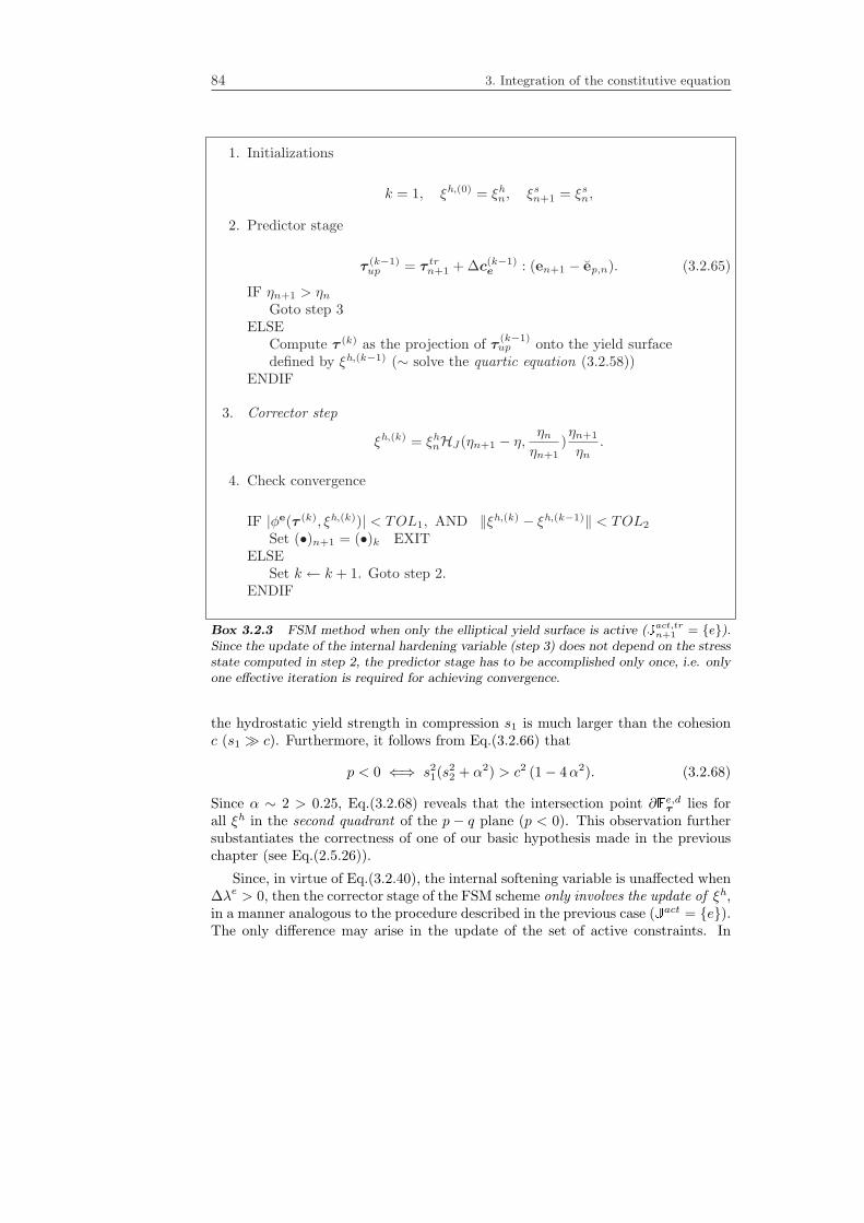
84 3. Integration of the constitutive equation
1. Initializations
k = 1, ξh,(0) = ξhn, ξsn+1 = ξsn,
2. Predictor stage
τ (k−1)up = τ trn+1 + ∆c(k−1)
e : (en+1 − ep,n). (3.2.65)
IF ηn+1 > ηnGoto step 3
ELSECompute τ (k) as the projection of τ
(k−1)up onto the yield surface
defined by ξh,(k−1) (∼ solve the quartic equation (3.2.58))ENDIF
3. Corrector step
ξh,(k) = ξhnHJ(ηn+1 − η, ηnηn+1
)ηn+1
ηn.
4. Check convergence
IF |φe(τ (k), ξh,(k))| < TOL1, AND ‖ξh,(k) − ξh,(k−1)‖ < TOL2
Set (•)n+1 = (•)k EXITELSE
Set k ← k + 1. Goto step 2.ENDIF
Box 3.2.3 FSM method when only the elliptical yield surface is active (Jact,trn+1 = e).Since the update of the internal hardening variable (step 3) does not depend on the stressstate computed in step 2, the predictor stage has to be accomplished only once, i.e. onlyone effective iteration is required for achieving convergence.
the hydrostatic yield strength in compression s1 is much larger than the cohesionc (s1 À c). Furthermore, it follows from Eq.(3.2.66) that
p < 0 ⇐⇒ s21(s22 + α2) > c2 (1− 4α2). (3.2.68)
Since α ∼ 2 > 0.25, Eq.(3.2.68) reveals that the intersection point ∂Ee,dτ lies forall ξh in the second quadrant of the p − q plane (p < 0). This observation furthersubstantiates the correctness of one of our basic hypothesis made in the previouschapter (see Eq.(2.5.26)).
Since, in virtue of Eq.(3.2.40), the internal softening variable is unaffected when∆λe > 0, then the corrector stage of the FSM scheme only involves the update of ξh,in a manner analogous to the procedure described in the previous case (Jact = e).The only difference may arise in the update of the set of active constraints. In
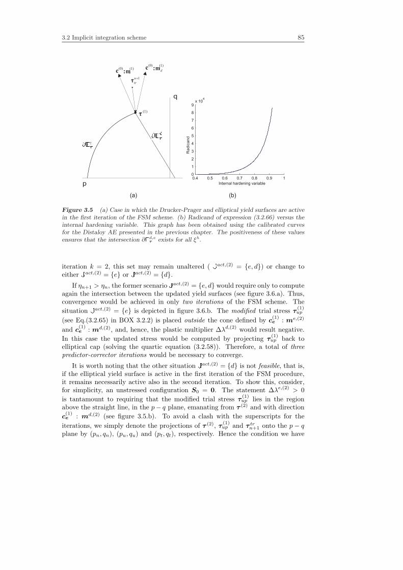
3.2 Implicit integration scheme 85
q
p0.4 0.5 0.6 0.7 0.8 0.9 10
1
2
3
4
5
6
7
8
9x 10
4
1n
tr
+
τ
em(0)
c :(1)
dm
(0)c :
(1)
(1)τ
Internal hardening variableR
ad
ica
nd
(a) (b)
Figure 3.5 (a) Case in which the Drucker-Prager and elliptical yield surfaces are activein the first iteration of the FSM scheme. (b) Radicand of expression (3.2.66) versus theinternal hardening variable. This graph has been obtained using the calibrated curvesfor the Distaloy AE presented in the previous chapter. The positiveness of these valuesensures that the intersection ∂Ed,eτ exists for all ξh.
iteration k = 2, this set may remain unaltered ( Jact,(2) = e, d) or change toeither Jact,(2) = e or Jact,(2) = d.
If ηn+1 > ηn, the former scenario Jact,(2) = e, d would require only to computeagain the intersection between the updated yield surfaces (see figure 3.6.a). Thus,convergence would be achieved in only two iterations of the FSM scheme. Thesituation Jact,(2) = e is depicted in figure 3.6.b. The modified trial stress τ
(1)up
(see Eq.(3.2.65) in BOX 3.2.2) is placed outside the cone defined by c(1)e : me,(2)
and c(1)e : md,(2), and, hence, the plastic multiplier ∆λd,(2) would result negative.
In this case the updated stress would be computed by projecting τ(1)up back to
elliptical cap (solving the quartic equation (3.2.58)). Therefore, a total of threepredictor-corrector iterations would be necessary to converge.
It is worth noting that the other situation Jact,(2) = d is not feasible, that is,if the elliptical yield surface is active in the first iteration of the FSM procedure,it remains necessarily active also in the second iteration. To show this, consider,for simplicity, an unstressed configuration S0 = 0. The statement ∆λe,(2) > 0is tantamount to requiring that the modified trial stress τ
(1)up lies in the region
above the straight line, in the p− q plane, emanating from τ (2) and with directionc(1)e : md,(2) (see figure 3.5.b). To avoid a clash with the superscripts for the
iterations, we simply denote the projections of τ (2), τ(1)up and τ trn+1 onto the p − q
plane by (pn, qn), (pu, qu) and (pt, qt), respectively. Hence the condition we have

86 3. Integration of the constitutive equation
to ascertain can be write as
qu ≥ qn + a (pn − pu), (3.2.69)
wherein a denotes the slope of the line a = κeγcα/(2µequ) > 0. From expressions(3.2.62) and (3.2.63), it follows that
pt = κentr en+1 − ep,n, pu = κen+1tr en+1 − ep,n, (3.2.70)
qt = 2µen‖deven+1 − ep,n‖, qu = µen+1‖dev en+1 − ep,n‖, (3.2.71)
and, thus,
qt =EenEen+1
qu = b qu, pt =EenEen+1
pu = b pu, (3.2.72)
for the Poisson’s ratio is constant and so the quotient κen/κen+1 is directly Een/E
en+1 =
b > 0. By substituting Eq.(3.2.72) into inequality (3.2.69), and upon rearrange-ment, we are led to
(qt −
(qn + a (pt − pn)
))+ b (qt + a pt) ≥ 0. (3.2.73)
Since ∆λe,(1) > 0, the following inequality holds
qt −(qn + a (pt − pn)
) ≥ 0, (3.2.74)
and hence the first term on the right-hand side of (3.2.73) is always non-negative.To prove that the other term is also non-negative, consider the limit case in whichqt = qn + a (pn − pt). In this instance, inequality (3.2.73) takes the form
b (qn − a pn) ≥ 0. (3.2.75)
For the above inequality to hold for all a, b > 0, it is sufficient that pn < 0, i.e., theintersection ∂Ed,eτ must lie in the second-quadrant of the p−q plane. This conditionis always satisfied, as stated in Eq.(3.2.68).
In conclusion, the solution of the return-mapping algorithm when the Drucker-Prager yield surface and the elliptical yield surface are involved is unique, and canbe obtained only in two or three iterations of the FSM predictor-corrector scheme.This conclusion can be also extended to cover the case in which the elliptical and theVon Mises yield surfaces may be active, by simply noting that the yield conditionrepresented by the Von-Mises surface is a degenerate case (α = γ = 0) of theDrucker-Prager yield condition.
CASE III : Drucker-Prager and Von Mises yield surface
Consider a stress state such that Jact,(1) = d, v. Computing the updatedstress state in this case is trivial, since it does not require any further labor otherthan determining the intersection between both the Drucker-Prager surface andthe Von-Mises surface:
qd,v = cv(ξhn), (3.2.76)

3.2 Implicit integration scheme 87
q
p
1n
tr
+
τ
(1)
upτ
e dm m
(1) (1)c c: :
(a)
(1)
τ
(2)
τn+1
τ =
n
1n+1
1-s-s
(2) (2)
dm(0)
c :(1)
em(0)
c :(1)
q1n
tr
+
τ
(1)
upτ
e dm m
(1) (1)c c: :
(1)
τ
(2)
τn+1
τ = (3)
τn+1
τ =
(2) (2)
dm(0)
c :(1)
em(0)
c :(1)
q
p
e
d
mm
(1)
(1)cc
::
(b)
(1)
τ
n
1n+1
1-s-s
(2)
(2)
1n
tr
+
τ
(1)
upτ
e
d
mm
(1)
(1)cc
::
(1)
τ
(2)
τ
(2)
(2)
Figure 3.6 (a) Case in which the Drucker-Prager and elliptical yield surfaces are activein the second iteration. (b) Case in which only the elliptical yield surface is active afterperforming the predictor step of the second iteration.
pd,v = (c(ξhn)− qd,v)/α, (3.2.77)
where (pd,v, qd,v) denotes the intersection between both surfaces. Recall that thisaspect of simplicity stems from the modification of the evolution equation for theinternal softening variable proposed in subsection 3.2.1.2.
CASE IV : Drucker-Prager yield surface
The remaining situation is that in which only the Drucker-Prager yield surfaceis active, that is, Jact,trn+1 = Jact,(k) = d, for all k = 1, 2 . . . The evolution equationsEq.(3.2.46) and Eq.(3.2.47) suggest that the internal hardening variable remains inits converged value, ξhn+1 = ξhn, whereas the softening variable evolves according to:
ξsn+1 = ξsn + 2 ∆λdn+1 qn+1. (3.2.78)
The above equation clearly shows that the update of ξs depends on the currentstress through its deviatoric part qn+1. Therefore, the return mapping algorithmcannot be handled exactly in a finite number of iterations, in contrast to the situa-tions encountered in cases I, II and III. Our concern here is to check if the sequencedefined by the predictor-corrector FSM scheme is convergent to an unique solu-tion, and to analyze the conditions under which such convergence, if any, can beguaranteed.
The equations for the predictor stage are obtained by projecting Eq.(3.2.43)(see BOX 3.2.2) onto the p− q plane:
p(k) = ptrn+1 −∆λd,(k) κen γ αc(k−1), (3.2.79)

88 3. Integration of the constitutive equation
q(k) =qtrn+1
1 + 4µen ∆λd,(k), (3.2.80)
φd,(k) = q(k) + αp(k) − c(k−1) = 0. (3.2.81)
After some algebra, the above system of equations can be reduced to the followingquadratic polynomial in q(k):
Γ(q(k)) = q(k)2
+(αptrn+1 + c(k−1)(χ− 1)
)q(k) − χ c(k−1)qtrn+1 = 0, (3.2.82)
whereχ = α2γ
κe
4µe. (3.2.83)
As ∆λd,(k) ≥ 0, it follows from Eq.(3.2.80) that q(k) ∈ [0, qtrn+1]. EvaluatingEq.(3.2.82) at q(k) = 0 yields
Γ(0) = −χ c(k−1)qtrn+1, (3.2.84)
All the variables appearing in the above are positive, hence Γ(0) ≤ 0 for all c(k−1) ≥0. Similarly, at q(k) = qtrn+1 we have
Γ(qtrn+1) = qtrn+1 (qtrn+1+αptrn+1−c(k−1)) ≥ qtrn+1 (
φd,trn+1︷ ︸︸ ︷
qtrn+1 + αptrn+1 − cn) > 0, (3.2.85)
since c(k−1) ≤ cn and φd,trn+1 > 0. Therefore, from the intermediate value theorem wededuce that the quadratic equation Eq.(3.2.82) have only one root in the interval[0, qtrn+1], and, consequently, the solution τ (k) to the system of equations of thepredictor step is unique.
The update of the internal softening variable that characterize the correctorstep can be directly inferred from Eq.(3.2.78):
ξs,(k) = ξsn + 2 ∆λd(ξs,(k), τ (k)) q(k). (3.2.86)
It is important to observe that ∆λd(ξs,(k), τ (k)) 6= ∆λd,(k), that is, the plasticmultiplier ∆λd,(k) arising from the solution of the predictor step is not used forupdating the internal variable. The only information from the predictor step em-ployed to correct the internal variables is the stress state τ (k). With this in mind,∆λd(ξs,(k), τ (k)) is obtained from Eq.(3.2.80) and then substituted in Eq.(3.2.78),leading to
ξs,(k) = ξsn +qtrn+1 − q(k)
2µen. (3.2.87)
The predictor equation (3.2.82) depends on ξs,(k−1) through the cohesion c(k−1).It is expedient, thus, to invoke the constitutive law (3.2.9) and recast Eq.(3.2.87)also in terms of c(k):
c(k) = cn +H(k)(ξs,(k) − ξsn) = cn +H(k)
2µen(qtrn+1 − q(k)). (3.2.88)
3.2 Implicit integration scheme 89
Recall (see Eq.(2.5.80) in section 2.5.5) that the expression for the exponentialsoftening modulus H(k) is given by:
H(k) = H0(ξhn)c(k)
c0(ξhn)= Hn
0
c(k)
cnh. (3.2.89)
Finally, Eq.(3.2.89) is inserted into Eq.(3.2.88). Upon rearrangement, one obtainsthe following expression for the update of cohesion:
Θcr = c(k) =cn
1− Hn0
cnh(qtrn+1 − q(k))
=cn
1 +|Hn
0 |cnh
(qtrn+1 − q(k)), (3.2.90)
with Hn0 defined as a dimensionless softening parameter:
Hn0 =
Hn0
2µen. (3.2.91)
3.2.2.1 Convergence analysis
Equation (3.2.82), corresponding to the predictor stage, can be conveniently rephrasedas:
Θpd = c(k−1) =q(k)(q(k) + αptrn+1)
12χ(qtrn+1 − q(k)) + q(k)
. (3.2.92)
Note that, according to the above equation,
Θpd = c(k−1) ≥ 0 ⇔ q ≥ qmin = max(0,−αptrn+1). (3.2.93)
Hence the solution qn+1 necessarily lies in the interval [qmin, qtrn+1]. Likewise, sinceqn+1 ∈ [qmin, qtrn+1], it follows immediately from Eq.(3.2.90) that c(k) ∈ [cmin, cn],where
cmin =cn
1 +|Hn
0 |cnh
(qtrn+1 − qmin). (3.2.94)
Inspection of Eq.(3.2.90) and Eq.(3.2.92) indicates that the problem can beposed in the alternative form of finding the limit of the sequence q(k) defined bythe recursion formula:
Θpd(q(k+1)) = Θcr(q(k)), (3.2.95)
that is,
q(k+1)(q(k+1) + αptrn+1)12χ(qtrn+1 − q(k+1)) + q(k+1)
=cn
1 +|Hn
0 |cnh
(qtrn+1 − q(k)), (3.2.96)
with q(0) = qtrn+1.

90 3. Integration of the constitutive equation
Sufficient conditions for convergence
Our concern now is to analyze the properties of this sequence. The next resultestablishes sufficient conditions for convergence11.
Proposition 3.2.3. Let q(k) be the sequence defined by the recursion formula
Θpd(q(k+1)) = Θcr(q(k)), q(0) = qtrn+1.
Assume that:
I) Θpd(q) and Θcr(q) are continuously differentiable in [qmin, qtrn+1].
II) Θpd(q) and Θcr(q) are monotonically increasing functions, i.e Θpd(q) ≥ 0 andΘcr(q) ≥ 0, ∀q ∈ [qmin, qtrn+1].
III) Θpd(qtrn+1) ≥ Θcr(qtrn+1) and Θpd(qmin) ≤ Θcr(qmin).
IV) There exists an unique solution q∗ in the interval [qmin, qtrn+1] to the equationΘpd = Θcr.
Then, the sequence q(k) converges to q∗.
Proof. The proof is carried out by showing that q(k) is a bounded monotonic(decreasing) sequence. In virtue of assumption I, we can expand Θpd(q(k+1)) andΘpd(q(k+1)) in Taylor series about q(k):
Θpd(q(k+1)) = Θpd(q(k)) + Θpd(ηp)(q(k+1) − q(k)), ηp ∈ [q(k+1), q(k)], (3.2.97)
Θcr(q(k+1)) = Θcr(q(k)) + Θcr(ηc)(q(k+1) − q(k)), ηc ∈ [q(k+1), q(k)]. (3.2.98)
Employing the recursion formula, we may write the above equations as
Θcr(q(k))−Θpd(q(k)) = Θpd(ηp)(q(k+1) − q(k)), ηp ∈ [q(k+1), q(k)], (3.2.99)
Θcr(q(k+1))−Θpd(q(k+1)) = Θcr(ηc)(q(k+1) − q(k)), ηc ∈ [q(k+1), q(k)]. (3.2.100)
The monotonic character of q(k), i.e. q(k+1) ≤ q(k) for all k = 0, 1, 2 . . . is provedby induction on k. The result holds trivially for k = 0, q(1) ≤ q(0), as can bededuced from assumptions II and III and by evaluating Eq.(3.2.99):
Θcr(q(0))−Θpd(q(0)) = Θpd(ηp)(q(1) − q(0))⇒Θcr(qtrn+1)−Θpd(qtrn+1) ≤ 0, Θpd(ηp) ≥ 0 ⇒ q(1) ≤ q(0).
(3.2.101)
Therefore, assume now that the result is also true for some k = i, that is, q(i) ≤q(i−1). Combining Eq.(3.2.99) and Eq.(3.2.100) we get
q(i+1) − q(i) =Θcr(ηc)Θpd(ηp)
(q(i) − q(i−1)). (3.2.102)
11These conditions only applies when softening is involved.

3.2 Implicit integration scheme 91
Since both Θcr and Θpd are nonnegative for all q ∈ [qmin, qtrn+1] (assumption II), itfollows immediately that q(i+1) − q(i) ≤ 0.
To complete the proof, we shall show that q(k) ∈ [qmin, qtrn+1] for all k, i.e.the sequence is bounded, and hence convergent. To this end, we shall argue bycontradiction. Suppose that there exists k > 0 such that q(k) ∈ [qmin, q∗]. FromEq.(3.2.99), the following property can be deduced:
Θcr(q(k)) ≤ Θpd(q(k)), (3.2.103)
for all k. Since from assumption III Θpd(qmin) −Θcr(qmin) ≤ 0, we know by theintermediate value problem that Θpd − Θcr has a zero in [qmin, q(k)], a fact thatcontradicts assumption IV , hence q(k) ∈ [qmin, qtrn+1] for all k. Furthermore, sincethe sequence is decreasing, it follows immediately that q∗ is its limit, as asserted.
¤
We are now confronted with the task of ascertaining whether the particularfunctional forms of Θcr and Θpd (see Eqs. (3.2.92) and (3.2.90), respectively) satisfythe sufficient conditions listed in the foregoing result. In regards to the condition ofcontinuity and differentiability, notice that both Θpd and Θcr are rational functionsof q:
Θpd =Npd(q)Dpd(q)
, Θcr =NcrDcr(q)
. (3.2.104)
Since Dcr(q) 6= 0 for all q ∈ [qmin, qtrn+1], Θcr(q) is continuously differentiable onthe interval [qmin, qtrn+1]. For qtrn+1 = 0, the predictor function Θpd has a singularityat q = 0, i.e. Dpd(0) = 0. However, as it may inferred from Eqs. (3.2.82) and(3.2.88), in this case the solution to the return mapping algorithm is trivial, sincethe internal variable does not evolve and the trial stress is simply “returned” tothe Drucker-Prager apex, i.e.:
qtrn+1 = 0 =⇒ qn+1 = 0, cn+1 = cn, pn+1 =cnα. (3.2.105)
Thus, in order to ensure also the continuity and differentiability of Θpd, the partic-ular case qtrn+1 = 0 will be excluded from the analysis.
Condition II states that Θcr(q) ≥ 0 and Θpd(q) ≥ 0. The verification for Θcr
is straightforward:
Θcr(q) =cn |Hn
0 |
cnh(1 +|Hn
0 |cnh
(qtrn+1 − q(k)))2
≥ 0, ∀q. (3.2.106)
To study the sign of the derivative of Θpd, we can write
Θpd(q) =q
12χ(qtrn+1 − q) + q
(q + αptrn+1) = F (q) (q + αptrn+1), (3.2.107)

92 3. Integration of the constitutive equation
where F (q) ∈ [0, 1] for q ∈ [qmin, qtrn+1]. Using the product rule, we get
Θpd(q) = F (
>0︷ ︸︸ ︷q + αptrn+1) + F. (3.2.108)
Since χ ≥ 0, the derivative of F :
F =12
χ qtrn+1(12χ(qtrn+1 − q) + q
)2, (3.2.109)
is also positive for all q. Hence, it follows from Eq.(3.2.108) that Θpd(q) ≥ 0 for allq ∈ [qmin, qtrn+1].
The condition III at the extremes of the interval is also satisfied:
Θpd(qtrn+1)−Θcr(qtrn+1) = qtrn+1 + αptrn+1 − cn = φd,trn+1 > 0 (3.2.110)
Θpd(qmin)−Θcr(qmin) = 0− cn
1 +|Hn
0 |cnh
(qtrn+1 − qmin)≤ 0. (3.2.111)
Finally, we prove in the following that the function Θ(q) = Θpd(q) − Θcr(q)has an unique zero in the interval [qmin, qtrn+1] (condition IV ). In turn, this resultprovides the assurance that there exists12 an unique solution to the return mappingalgorithm when Jact,trn+1 = d.
Proposition 3.2.4. The function defined as Θ(q) = Θpd(q) − Θcr(q), with Θpd
and Θpd given in Eq.(3.2.90) and Eq.(3.2.92), respectively, has an unique zero inthe interval [qmin, qtrn+1].
Proof. Multiplying Θ = 0 by the denominators of Θpd and Θcr (which are non-vanishing ∀ q ∈ [qmin, qtrn+1]), a cubic polynomial R(q) =
∑3i=0 ri q
i = 0 is obtained.After elementary manipulations, the coefficients (ri, i = 0 . . . 3) are found to begiven by:
r3 = −|Hn0 |cnh
, r2 = (1 +|Hn
0 |cnh
(qtrn+1 − αptrn+1)), (3.2.112)
r0 = −12cnq
trn+1χ, r1 = r2 − cn(1− 1
2χ). (3.2.113)
12In proposition 3.2.4 it is shown that the norm of the updated deviatoric stress tensor canbe obtained by finding the root of a cubic equation in [qmin, q
trn+1]. Hence, the return mapping
problem when Jact,trn+1 = d can be viewed also as a root finding problem. This root may beobtained by other numerical means, such as the closed-form expressions based on Cardano’smethod [87], or variants thereof, and not necessarily by the proposed method. Nonetheless,for completeness, the convergence properties of the sequence defined by the FSM algorithm isdiscussed herein.

3.2 Implicit integration scheme 93
Evaluation of the polynomial R at the extremes of the interval yields
R(qmin) = −cn (
>0︷ ︸︸ ︷12χ(qtrn+1 − qmin) + qmin) ≤ 0, (3.2.114)
R(qtrn+1) = qtrn+1(qtrn+1 + αptrn+1)− cn = qtrn+1 φ
d,trn+1 ≥ 0. (3.2.115)
Thus, since R(qmin) and R(qtrn+1) have opposite signs, we know by the intermediatevalue theorem that there exist n roots of R in [qmin, qtrn+1], with n = 1 or n = 3.The signs of r0 and r3 indicate that R(0) < 0 and R(−∞) > 0. Therefore, followingthe same logic as above, R = 0 have m negative roots, with m = 1 or m = 3. Ifwe suppose that n = 3, then the total number of zeros would be n + m = 4 orn + m = 6, which cannot be true, since the polynomial is cubic. Hence, R hasonly one root in [qmin, qtrn+1], and, consequently, Θ possesses an unique zero in[qmin, qtrn+1], as asserted. ¤
(0)
(3)
(4)
(0)
(1)
(2)
q
(1)q
(2)q
c
c
c
1qtr
n+
Norm of deviatoric stress (q)Norm of deviatoric stress (q)
cC
ohesio
n (
)
0pd
Q =Predictor s. ( )
0cr
Q =Corrector s. ( )
1cn+
1qn+minq
minc
1
, cn n
dtr
+f +
cn
(3)c(4)c
Figure 3.7 Linearly convergent FSM sequence.
Therefore, we conclude that the functional forms of Θcr and Θpd, given inEq.(3.2.90) and Eq.(3.2.92), respectively, fulfill the sufficient conditions for thesequence defined by the recursion formula (3.2.95) to converge. As a corollary,we can say that the FSM algorithm for the case Jact,trn+1 = d converges to thesolution of the return mapping algorithm regardless of the location of the trial stress(ptrn+1, q
trn+1) and the value of the material parameters χ, α and Hn
0 . It is worthnoting that no restriction is placed on the amount of allowable softening, symbolizedby Hn
0 , which is one of the drawbacks that plague elastic-plastic models equippedwith softening [92].

94 3. Integration of the constitutive equation
Rate of convergence
To assess the computational efficiency of the FSM algorithm, it is of paramountinterest to study its rate of convergence. The following result address this question.
Proposition 3.2.5. Let q(k) be the convergent sequence defined by the recursionformula Θpd(q(k+1)) = Θcr(q(k)). Let q∗ denote the limit of this sequence andconsider an interval [q∗, β] ⊂ [q∗, qtrn+1] such that
Θpd(η)Θcr(η)
< 1, (3.2.116)
for all η ∈ [q∗, β]. Let N be a positive integer such that q(N) ≤ β. Then, the error,denoted as e = q−q∗, decreases for all k ≥ N , being the rate of this decrease linear.
Proof. Expressing Θpd(q(k+1)) and Θcr(q(k)) in Taylor series about q∗ andtruncating after the first order term yields:
Θpd(q(k+1)) = Θpd(q∗) + Θpd(ηp)(
e(k+1)
︷ ︸︸ ︷q(k+1) − q(q∗)), ηp ∈ [q∗, q(k+1)], (3.2.117)
and
Θcr(q(k)) = Θcr(q∗) + Θcr(ηc)(
e(k)
︷ ︸︸ ︷q(k+1) − q(k)), ηc ∈ [q∗, q(k)], (3.2.118)
respectively. Subtracting Eq.(3.2.118) from Eq.(3.2.117) gives:
Θpd(q(k+1))−Θcr(q(k)) =(Θpd(q∗)−Θcr(q∗)
)
+ Θpd(ηp) e(k+1) − Θcr(ηc) e(k).(3.2.119)
Since Θpd(q∗) = Θcr(q∗) and Θpd(q(k+1)) = Θcr(q(k)) , after solving for e(k+1) weget
e(k+1) =Θcr(ηc)Θpd(ηp)
e(k). (3.2.120)
For k > N , q(k), q(k−1) ∈ [q∗, β]. Then, the error decreases by a factor Θcr(ηp)/Θpd(ηc),ηp ∈ [q∗, q(k+1)], ηc ∈ [q∗, q(k)]. Eq.(3.2.120) further shows that e(k+1) depends lin-early on e(k). ¤
Thus, the above proposition shows that the rate of convergence is linear in aneighborhood of the solution in which Θcr > Θpd. It is straightforward to prove,by contradiction, that this condition of greater slope of the predictor curve in some[q∗, β], β ∈ [0, qtrn+1 − q∗] always holds. Suppose that Θcr(q∗) < Θpd(q∗). Thecontinuity assumption implies that for some ε > 0 Θpd(q∗+ ε) < Θcr(q∗+ ε), whichis a contradiction, since Θpd(q) ≥ Θcr(q) for all q ∈ [q∗, qtrn+1].

3.2 Implicit integration scheme 95
The so-called asymptotic convergence factor [87] Θcr/Θpd can be estimatedgrossly using the mean value theorem:
Θcr
Θpd=
Θcr(qtrn+1)−Θcr(qmin)Θpd(qtrn+1)−Θpd(qmin)
=|Hn
0 |/cnh(qtrn+1 − qmin)1 + |Hn
0 |/cnh(qtrn+1 − qmin)1
φd,trn+1
cn+ 1
.(3.2.121)
This estimation reveals that the asymptotic convergence factor is inversely propor-tional to the yield equation evaluated at the trial stress φd,trn+1. Hence the FSMalgorithm converges more rapidly with trial stresses located far from the yield sur-face (φd,trn+1 À cn), since in this case Θcr/Θpd approaches zero.
(0)
(1)q
(2)q
(3)q
(4)q
c
(1)c
(2)c
1qtr
n+
Norm of deviatoric stress (q)Norm of deviatoric stress (q)
cC
ohesio
n (
)
0pd
Q =Predictor s. ( )
0cr
Q =Corrector s. ( )
1cn+
1qn+minq
minc
1
, cn n
dtr
+f +
cn
(3)c(4)c
Figure 3.8 Quadratically convergent FSM sequence.
The conclusion that can be drawn from the preceding discussion is that the FSMalgorithm offers a remarkable aspect of robustness, inasmuch as it converges to thesolution regardless of the values of the material properties, and furthermore, itsconvergence is even faster when the trial stress is placed far from the yield surface.Nevertheless, it is natural to inquire at this point whether other schemes, viewedalso in the light of the predictor-corrector methodology, might exhibit higher ratesof convergence. To assist in the answering of this question, it proves helpful to,first, illustrate graphically the performance of the standard FSM method. In figure3.7 the predictor and corrector equations Θpd = 0 and Θcr = 0 are represented inthe c− q plane. The predictor step consists in finding the intersection between thehorizontal lines (c constant) and the predictor curve Θpd = 0. The corrector step,

96 3. Integration of the constitutive equation
on the other hand, involves solving the intersection of the corrector graph Θcr = 0and the vertical lines (q constant).
The plot in figure 3.8 clearly identifies the strategy to follow in arriving at aFSM algorithm with a higher rate of convergence. The predictor stage would remainunaltered (projection onto the yield surface with c constant), whereas the correctorstep would be modified and accomplished by finding the intersection between thecurve Θcr = 0 and the straight line tangent to Θpd = 0 at q(k−1). The correspondingsequence is defined by the recursion formulae:
Θpd(q(2k−1)) = Θcr(q(2k−2)), (3.2.122)
Θcr(q(2k)) = Θpd(q(2k−1)) + Θpd(q(2k−1))(q(2k) − q(2k−1)), (3.2.123)
with k = 1, 2 . . . and q(0). The analysis of the convergence of this sequence isundertaken in a similar manner to that presented in proposition 3.2.5.13 We simplyquote the final result (for k →∞):
e(2k−1) =Θcr(q∗)Θpd(q∗)
e(2k−2), (3.2.124)
e(2k) =12
Θcr(q∗)Θpd(q∗)− Θcr(q∗)
e2(2k−1). (3.2.125)
Combining Eqs. (3.2.124) and (3.2.125), we get
e(2k) =12
Θcr(q∗)Θpd(q∗)− Θcr(q∗)
(Θcr(q∗)Θpd(q∗)
)2
e2(2k−2). (3.2.126)
The above equation reveals that the rate of convergence of this modified FSMalgorithm is quadratic. However, in return for its enhanced convergence, a necessarycondition for the sequence defined by Eqs. (3.2.124) and (3.2.125) to be monotonicdecreasing is that Θpd > 0 in a neighborhood of the solution, i.e., the predictorfunction must be convex. To check if this condition is satisfied, Eq.(3.2.108) isdifferentiated with respect to q, yielding
Θpd = 2F + F (q + αptrn+1). (3.2.127)
After some manipulation, F can be expressed as
F =−2 (1− 1/2χ)
q(1− 1/2χ) + 1/2χqtrn+1
F . (3.2.128)
Substitution of the above into Eq.(3.2.127) leads to
Θpd = 2F(1− − (1− 1/2χ)
q(1− 1/2χ) + 1/2χqtrn+1
(q + αptrn+1)). (3.2.129)
13The only difference lies in that, in Eq.(3.2.123), Θpd(q(2k−1)) is expanded in a Taylor series
around q∗ up to the second order term.

3.3 IMPLEX integration scheme 97
So the predictor function is convex whenever the following inequality is satisfied:
1 >(1− 1/2χ)
q(1− 1/2χ) + 1/2χqtrn+1
(q + αptrn+1), (3.2.130)
which, upon rearranging, gives
12χ(qtrn+1 + αptrn+1)− αptrn+1 > 0. (3.2.131)
It follows from the preceding equation that the convexity condition cannot be guar-anteed for any admissible values of the trial stress and the material parameter χ.Only for ptrn+1 < 0 the above inequality holds regardless of the value of χ.
In conclusion, we have seen that, by simply modifying the equation for theupdate of cohesion in the corrector step, it is plausible to devise a quadraticallyconvergent method preserving the predictor-corrector character. This modification,in turn, involves the linearization of the predictor function, and as a consequence,the convexity of this function appears as an additional requirement for convergence.However, inequality (3.2.131) clearly shows that this condition cannot be ensuredfor all conceivable trial stress states. Therefore, in the interest of robustness, thisappealing quadratically convergent FSM scheme is abandoned in favor of the ori-ginal linearly converging one.
3.3 IMPLEX integration scheme
The arguments in support of the implicit-explicit (IMPLEX) integration schemewere already put forward in subsection 3.1.1. Here we simply choose those variablesto be treated explicitly and derive the stress update and the algorithmic tangentmodulus arising from this choice. The reader is referred to the work of Oliver etal. [79, 80] for further details on the structure of this integration scheme.
By definition, the internal variables are monotonically increasing functions oftime, i.e. ξ ≥ 0. For this reason, they are logical candidates to be treated explicitly,since its evolution can be predicted more accurately than other variables exhibit-ing non-monotonic behavior. The following analysis pursues, thus, to develop anexpression for explicitly updating the set of internal variable at tn+1 using valuesobtained in previous time steps by an implicit integration procedure.
To this end, consider first the Taylor expansion of the exact solution, denotedby an overbar on the symbol for the internal hardening, to the governing differentialequation at tn−1 around tn:
ξn−1 = ξn +∂ξ
∂t
∣∣∣∣ξn
(tn−1 − tn) +O(∆2tn), (3.3.1)
or alternatively,
ξn = ξn−1 +∂ξ
∂t
∣∣∣∣ξn
∆tn +O(∆2tn), (3.3.2)

98 3. Integration of the constitutive equation
where∂ξ
∂t
∣∣∣∣ξn
= ξ(ξn, τn). (3.3.3)
Next, the Taylor expansion is carried out again around tn, but evaluated at tn+1,yielding
ξn+1 = ξn +∂ξ
∂t
∣∣∣∣ξn
∆tn+1 +O(∆2tn+1). (3.3.4)
If the remainder term O(∆2tn+1) is truncated in the above equation, then the re-sulting expression would correspond to a standard explicit finite difference equation.The application of the above explicit difference equation for marching the solutionforward from one time level to the next time level presents the inconvenience that,since the yield condition is not enforced at tn+1, the error would accumulate andthe yield condition may be substantially violated, leading to updated stress pro-hibitively far from the yield surface. In order to avoid that this drift from theyield surface grows unboundedly, Oliver et al.[79, 80] propose to approximate thederivative in Eq.(3.3.4) using the derivative appearing in expression Eq.(3.3.2).Therefore, truncating the term O(∆2tn) in Eq.(3.3.2), one gets
ξn = ξn−1 +∂ξ
∂t
∣∣∣∣ξn
∆tn, O(∆2tn). (3.3.5)
The above constitutes an implicit finite difference equation, in the sense thatthe internal variable at tn, ξhn, is obtained by an expression that uses a derivativeevaluated also at tn. Hence ξn−1 and ξn can be regarded as the values of the internalvariables obtained at times tn−1 and tn, respectively, by solving the return mappingalgorithm outlined in the previous section. From Eq.(3.3.5), we can deduce that
∂ξ
∂t
∣∣∣∣ξn
=ξn − ξn−1
∆tn, O(∆tn). (3.3.6)
Finally, inserting the above approximation into Eq.(3.3.4), and truncating the re-mainder term, yields
ξn+1 = ξn + (ξn − ξn−1)∆tn+1
∆tn, O(∆tn+1∆tn). (3.3.7)
This expression represents the update of the internal variables at tn+1 in terms ofimplicit values computed at tn and tn−1. The distinction between approximatedquantities stemming from the IMPLEX integration and from the pure implicitintegration schemes is made by attaching a tilde symbol over the IMPLEX variables.
Note that the IMPLEX algorithm is a multistep method, since two points (tnand tn−1) are used to advance the solution in time to point tn+1. The orderof the extrapolation represented by Eq.(3.3.7) can be increased by simply using ahigher-order approximation for the derivative at tn. However, accuracy assessmentscarried out by Oliver et al. [80] show that the benefits arising from this practiceare quite subtle and do not outweight the concomitant increase of computationalstorage requirements.

3.3 IMPLEX integration scheme 99
The set of state variables defining the size and shape of the yield surfaces canbe obtained at time tn+1 from the corresponding hardening/softening laws, usingthe vector of internal variables derived in Eq.(3.3.7) as argument, that is:
s1,n+1 = s1h(ξhn+1), s2,n+1 = s2h(ξhn+1), cv,n+1 = cvh(ξhn+1), (3.3.8)
cn+1 = cn +∂ch∂ξh
∣∣∣∣n+1
(ξhn+1 − ξhn) + Hn+1(ξsn+1 − ξsn), (3.3.9)
where
Hn+1 =cn+1
c0(ξhn+1)H0(ξhn+1). (3.3.10)
In regards to the plastic multipliers, the update suggested by Oliver et al. isalso adopted:
∆λβ
n+1 = ∆λβn∆tn+1
∆tn, β = e, d, v, (3.3.11)
i.e., the IMPLEX discrete plastic multiplier ∆λβ
n+1 at tn+1 is directly computedby multiplying the corresponding implicit discrete plastic multiplier at tn by thequotient ∆tn+1/∆tn. It should be mentioned, however, that the derivation ofthis update does not display the same mathematical rigor as the one presentedin Eq.(3.3.7) for the internal variables. This can be explained as follows. TheIMPLEX scheme was originally conceived for integrating numerically elastic-plasticconstitutive models with associated flow rules and a single internal variable [79].Under such conditions, and by properly defining the flow rule, the rate of changeof the internal variable can be identified with the continuum plastic multiplier,i.e., ξ = λ. In this instance, one can legitimately obtain the update as ∆λn+1 =∆λn∆tn+1/∆tn, since ∆λ = ∆ξ. In our case, by contrast, we have three plasticmultipliers and two independent internal variables whose evolution equations alsoinvolve stress measures, and thus, such identity cannot be established, hence thead-hoc character of the proposed update (3.3.11).
Notice that the extrapolation of the plastic multipliers does not entails allocatingadditional storage for implicit values at tn−1. Expression (3.3.11) also reveals thatthe elastic or inelastic nature of the response predicted by the IMPLEX integrationscheme at tn+1 is dictated by the response computed implicitly at tn. This maygive rise to numerical overshoots and oscillations in the transition from elastic toplastic conditions and vice versa. Schemes for adaptively controlling the length ofthe time step, also covered by the work of Oliver et al.[80], prove advantageous indiminishing the deleterious effects on the quality of the computed response of suchshortcomings.
Our developments in this section have been focused thus far on those variables(ξ and ∆λβ) whose updates can be handled explicitly. Attention is confined now tocompute the Kirchhoff stress tensor at tn+1. Since the concept of extrapolation isnot applied for such computation (stresses are treated implicitly), the methodologyfor deriving this update equation parallels that followed for devising Eq.(3.2.24) in

100 3. Integration of the constitutive equation
the implicit case. Thus, we can directly write
τn+1 = τ trn+1 + ∆ce,n+1 : (en+1 − ep,n)−3∑
β=1
∆λβ
n+1 ce,n+1 : mβn+1, (3.3.12)
where we have simply replaced the implicit quantities in Eq.(3.2.24) by IMPLEXquantities (with tilde). The fourth-order tensors ∆ce,n+1 and ce,n+1 are evaluatedas
∆ce,n+1 = ce(ξhn+1)− ce(ξhn), ce,n+1 = ce(ξhn+1), (3.3.13)
whereas the plastic flow vector is given by
mβn+1 = mβ(ξhn+1, τn+1). (3.3.14)
In general, obtaining τn+1 from Eq.(3.3.12) requires solving a non-linear tensorequation. However, as alluded to earlier (see Eq.(3.2.48)), in our case, the plasticflow vector on each surface is an affine transformation of the Kirchhoff stress tensor,i.e.,
mβn+1 = Aβ
n+1 : τn+1 + B,n+1 (3.3.15)
where the fourth-order and second-order tensors Aβn+1 and Bβ
n+1 are defined as
Aβn+1 = 2 Idev +
13uβn+1 1⊗ 1, (3.3.16)
Bβn+1 = vβn+1 1, (3.3.17)
respectively, with the yield surface dependent parameters uβn+1 and vβn+1, β =e, d, v, given by (see Eqs. (3.2.49) and (3.2.50)):
uen+1 =23(s2,n+1)2, udn+1 = uvn+1 = 0, (3.3.18)
ven+1 = vvn+1 = 0, vdn+1 =13γ cn+1 α. (3.3.19)
Substituting Eq.(3.3.15) into Eq.(3.3.12) and solving for τn+1 yields
τn+1 = R−1n+1 :
(τ trn+1 + ∆ce,n+1 : (en+1 − ep,n)−
ce,n+1 :3∑
β=1
∆λβ
n+1 Bβn+1
),
(3.3.20)
where
Rn+1 = I + ce,n+1 :3∑
β=1
∆λβ
n+1Aβn+1. (3.3.21)
Equation Eq.(3.3.20) constitutes a closed-form formula for the Kirchhoff stressupdate at tn+1. This update admits the following deviatoric-hydrostatic decompo-sition:
τn+1 = dev τn+1 + pn+1 1, (3.3.22)

3.3 IMPLEX integration scheme 101
where
dev τn+1 =dev τ trn+1 + 2∆µen+1 dev (en+1 − ep,n)
1 + 4 µen+1
∑3β=1 ∆λ
β
n+1
(3.3.23)
pn+1 =ptrn+1 + ∆κen+1 tr (en+1 − ep,n) + 3 κen+1
∑3β=1 ∆λ
β
n+1vβn+1
1− κen+1
∑3β=1 ∆λ
β
n+1uβn+1
. (3.3.24)
3.3.1 Algorithmic elastoplastic tangent moduli
Our emphasis so far has been entirely local, i.e., attention has been confined todetermine the local stress state at time tn+1, given a prescribed deformation stateand a set of initial data. However, the ultimate goal in the numerical simulation ofthe powder sub-system is to solve an initial boundary problem for the displacementfield. The numerical solution of this problem relies on the spatial discretization,via a Galerkin finite element projection, of the weak form of the momentum equa-tion. Due to the non-linear character of the problem, a time-discretization of thisvariational form is also necessary, and the response is finally obtained by solving asequence of linearized problems.
The theory underlying the spatial and time discretization, as well as the lin-earization of the resulting weak formulation are not addressed in this work. Thereader is referred to the vast literature on the subject [5, 113, 88] for further details.Here we limit ourselves to provide an expression for the algorithmic tangent moduli,which is a key step in the above mentioned linearization of the weak formulation.
The algorithmic tangent moduli is obtained merely by applying the directionalderivative relative to a strain increment to the update formulas of the integrationalgorithm [92]. In connection with this, we recall that the stress values furnishedby the IMPLEX integration scheme determine the internal forces appearing in theweak formulation of the problem. Hence we shall focus on the algorithmic tangentoperator consistent with this integration scheme.
In using the algorithmic tangent moduli on the computation of the response,one is tacitly assuming that the linearization is carried out after the stress-updatealgorithm is introduced [5]. Therefore, consider the term corresponding to theinternal forces of the total lagrangian weak form statement at time tn+1:
Gintϕn+1(Sn+1,η0) =
∫
Ω0
Fn+1 · Sn+1 ·Grad η0 dΩ. (3.3.25)
We shall not dwell on formal considerations concerning the above expression, suffi-cient be it to say that Grad η0 symbolizes the material gradient operator, definedin cartesian coordinates as
(Grad η0)aA =∂η0 a
∂XA. (3.3.26)
acting on the material test function η0, which, in turn, belongs to a proper space offunctions. The Second Piola-Kirchhoff stress tensor Sn+1 is the material counter-part of the spatial Kirchhoff stress tensor obtained by the IMPLEX stress-update

102 3. Integration of the constitutive equation
formula (3.3.20). Linearization about the current configuration Ωn+1 involves ob-taining the directional derivative of Eq.(3.3.25) in the direction of an incrementaldisplacement ∆U , that is,
D∆U Gintϕn+1(Sn+1,η0) =
∫
Ω0
D∆U Fn+1 · Sn+1 ·Grad η0 dΩ+∫
Ω0
Fn+1 ·D∆U Sn+1 ·Grad η0 dΩ.(3.3.27)
We restrict our attention to the second term on the right-hand side of the aboveequation, which after the finite element projection, gives rise to the so-called ma-terial stiffness matrix. From the definition of directional derivative, and by usingthe chain rule, we get
D∆U Sn+1 =d
dε
∣∣∣∣ε=0
(Sn+1(ϕn+1 + ε∆U)
)
= Cep,n+1 :d
dε
∣∣∣∣ε=0
(En+1(ϕn+1 + ε∆U)
),
(3.3.28)
where the components of the material algorithmic tangent moduli Cep,n+1 are givenby
(Cep,n+1)ABCD =(Sn+1)AB
(En+1)CD. (3.3.29)
Thus, Cep,n+1 can be derived by finding the operator satisfying
∂Sn+1
∂tn+1= Cep,n+1 :
∂En+1
∂tn+1. (3.3.30)
However, since the stress-update formula (3.3.20) is cast in terms of spatial quanti-ties, it is convenient to obtain first the spatial algorithmic tangent moduli cep,n+1,and then transforming this tensor into the reference configuration via a pull-backoperation.
The spatial algorithmic tangent moduli cep,n+1 is defined by the spatial coun-terpart of Eq.(3.3.30):
Lvτn+1 = cep,n+1 : Lven+1 = cep,n+1 : dn+1, (3.3.31)
wherein the Lie derivative Lv(•) is used to preserve objectivity. An expressionfor cep,n+1 is obtained by applying the Lie operator to the stress-update formulaEq.(3.3.20). The simplicity, in comparison to an standard implicit integrationscheme, afforded by the use of the IMPLEX stress-update scheme is manifestedby the fact that the derivative of the plastic multipliers and the internal variablesvanishes, in virtue of the extrapolated character of these variables, that is, ∆λ
β
n+1
and ξn+1 do not depend on the deformation state at tn+1. However, even withthis simplification, it takes tedious algebra to derive a closed-form expression for

3.3 IMPLEX integration scheme 103
cep,n+1. This derivation is hence relegated to Appendix (A.4), and we simplyrecord here the final expression, which takes the following form:
cep,n+1 = R−1n+1 :
(ae,n+1(ee,n+1) + ce,n+1 :
(I −
3∑
β=1
∆λβ
n+1zβn+1(τn+1)
).
(3.3.32)
The isotropic fourth order tensor Rn+1 was introduced when deriving the closedform expression for the stress-update (see Eq.(3.3.21)). On the other hand, thetensor ae,n+1(ee,n+1) is given by the following formula
ae,n+1(ee,n+1) = −2((κen+1−
23µen+1
)(1⊗ee,n+1+tr ee,n+1I
)+2 µen+1 Is(ee,n+1)
),
(3.3.33)where ee,n+1 is the elastic strain tensor computed as
ee,n+1 = en+1 −(ep,n +
3∑
β=1
∆λβ
n+1mβn+1
). (3.3.34)
and the operator Is(•) has the following component form:
(Is(•))abef =12((•)afδbe + (•)bfδae). (3.3.35)
The expression for zβn+1(τn+1) is given by
zβn+1(τn+1) = aτ,n+1(uβn+1, τn+1) + 2 vβn+1I, (3.3.36)
where the yield surface dependent parameters uβn+1 and vβn+1 were defined in Eqs.(3.3.18) and (3.3.19), respectively. The structure of tensor aτ,n+1 is rather similarto that of ae,n+1:
aτ,n+1(uβn+1, τn+1) = 2
(13(uβn+1−2
)(1⊗ τn+1 +tr τn+1I
)+4 Is(τn+1)
). (3.3.37)
Remark 3.3.1. The fourth order tensors ae,n+1(ee,n+1) and zβn+1(τn+1) arise fromapplying the Lie derivative to the metric tensor, which is involved in the definitionof both the elasticity tensor and the plastic flow vectors. Thus, if these terms arediscarded from Eq.(3.3.32), one obtains the algorithmic tangent operator for theIMPLEX integration scheme corresponding to a small strain formulation, since inthis kinematical approach the distinction between reference and current configura-tions are negligible for the purposes of computing stress and strain. The resultingexpression reads
cep,n+1|‖e‖¿1 = R−1n+1 : ce,n+1. (3.3.38)
Expanding this equation using Eq.(3.3.21) gives
cep,n+1|‖e‖¿1 = κimxn+1 1⊗ 1 + 2 µimxn+1 Idev, (3.3.39)

104 3. Integration of the constitutive equation
where
κimxn+1 =κen+1
1 + 3 κen+1
∑3β=1 ∆λ
β
n+1uβn+1
=κen+1
1 + 2 κen+1∆λe
n+1(s2,n+1)2
(3.3.40)
µimxn+1 =µen+1
1 + 4 µen+1
∑3β=1 ∆λ
β
n+1
(3.3.41)
Inspection of Eq.(3.3.39) indicates that, in the small strain setting, the algorithmictangent operator emanating from the IMPLEX integration scheme is an isotropictensor of rank 4, characterized by two parameters, which, in analogy to the no-tation for the elastic bulk and shear modulus, are denoted by κimxn+1 and µimxn+1.
Furthermore, since ∆λβ
n+1 ≥ 0, it follows from Eqs. (3.3.40) and Eq.(3.3.41) that
κimxn+1 ≤ κen+1, (3.3.42)
µimxn+1 ≤ µen+1, (3.3.43)
where the inequality or equality holds accordingly as the material is deformingplastically or elastically, respectively.
As alluded to in section 3.1.1, the development of the implicit-explicit integra-tion scheme was prompted by the need to enhance the spectral properties of thealgorithmic elastoplastic moduli, whose positive definiteness cannot be guaranteedwhen using an standard implicit integration scheme, mainly due to the presenceof strain softening. Since, according to Eqs. (3.3.40) and Eq.(3.3.41), κimxn+1 > 0and µimxn+1 > 0, it follows then that the algorithmic elastoplastic moduli shown inEq.(3.3.39) is positive-definite. Another remarkable property of this small strainalgorithmic operator is that it does not depend on the deformation state at tn+1,hence it turns out to be step-constant.
One can conclude from the foregoing remark that the positive-definiteness of thealgorithmic elastoplastic moduli is guaranteed in those situations in which a smallstrain kinematics is sufficient to yield a realistic description of the deformationstate. As pointed out in section 2.2.1, the ejection stage, which, in turn, is the partof the compaction cycle in which the compacted powder is more liable to developcracks, falls within this type of situations, since the magnitude of plastic and elasticstrains are relatively small, and, besides, the motion of the compact through thedie cavity during ejection involves no solid rigid rotations. Therefore, we can assertthat, in contrast to the situation that one would encounter if a standard implicitintegration scheme is employed, the numerical performace of the algorithm is notimpaired14by the presence of strain softening, at least in the computation of theresponse corresponding to the ejection stage.
14This is, of course, insofar as material non-linearities are concerned. The numerical per-formance may be seriously affected by the characteristics of the contact problem, specially thestick-slip behavior when Coulomb friction models are used.

3.3 IMPLEX integration scheme 105
To further improve the confidence in the numerical performace of this integra-tion scheme, the spectral properties of the (large strains) algorithmic elastoplastictensor shown in Eq.(3.3.32) should be also examined. As it may be surmised, arigorous analysis concerning the positive-definite character of cep,n+1 in a generalsituation, i.e., for any ee,n+1 and τn+1 entails substantial difficulties. An easierroute is to determine the order of magnitude of the tensors ae,n+1 and zβn+1, andsee if their influence in the value of cep,n+1 is significant.
Consider first a situation in which the response predicted by the integrationscheme is entirely elastic. In this case, the spatial elastoplastic tensor adopts theform:
cep,n+1|∆λβ=0 = ce,n+1 + ae,n+1(ee,n+1). (3.3.44)
According to expression (3.3.33), the order of magnitude of ae,n+1 is ‖ae,n+1‖ ∼Een+1 ‖ee,n+1‖, whereas ‖ce,n+1‖ ∼ Een+1. Hence,
ce,n+1
ae,n+1∼ ‖ee,n+1‖. (3.3.45)
By hypothesis, the extent of elastic strains is significantly less than unity (‖ee,n+1‖ ∼10−3, in accordance with data plotted in figure 3.2). We see thus that the contri-bution of ae in the computation of cep,n+1 is not significant15.
On the other hand, in the course of plastic deformation, the term involvingzβn+1, that is,
3∑
β=1
∆λβ
n+1zβn+1(τn+1), (3.3.46)
comes also into play. In this case, however, the task of disclosing whether theinfluence of this contribution is relatively important or not is by no means trivial,due mainly to the variability of the plastic multipliers ∆λ
β
n+1. We proceed firstby estimating the order of magnitude of zβn+1(τn+1). According to Eq.(3.3.36), wehave
‖zβn+1‖ ∼ max(‖aτ,n+1‖, ‖vβn+1‖). (3.3.47)
Using Eq.(3.3.37), we get
‖aτ,n+1(τn+1)‖ ∼ ‖uβn+1‖‖τn+1‖ ∼ ‖‖τn+1‖‖, (3.3.48)
since ‖uvn+1‖ = ‖udn+1‖ = 0 and s2 ∼ 1 (see figure 2.12), and, hence, ‖uen+1‖ ∼(s2,n+1)2 ∼ 1. Besides, taking into account Eq.(3.3.19):
vβn+1 ∼
0, if ∆λd
n+1 = 0,
α γ cn+1, if ∆λd
n+1 > 0.(3.3.49)
15Incidentally, if one discards the term ae from the definition of cep,n+1, then a hypoelasticconstitutive equation would be recovered, Lvτ = ce : Lvee

106 3. Integration of the constitutive equation
According to the empirical correlations set forth in the previous chapter, α ∼ 2,and γ is chosen close to zero, say γ ∼ 10−2, hence
vβn+1 ∼
0, if ∆λd
n+1 = 0,
10−2 cn+1, if ∆λd
n+1 > 0.(3.3.50)
Using estimations (3.3.48) and (3.3.50) in (3.3.47), we finally obtain
‖zβn+1‖ ∼‖τn+1‖, if ∆λ
d
n+1 = 0,
max(‖τn+1‖, 10−2 cn+1), if ∆λd
n+1 > 0.(3.3.51)
We concentrate our attention now in an estimation for the the plastic multipliers.The following expression for ∆λ
β
n+1 can be deduced from Eq.(3.3.11):
∆λβ
n+1 = ∆λβn∆tn+1
∆tn=
∆tn+1
∆tnqtrn − qn4µen qn
, β = e, d, v. (3.3.52)
The above expression becomes indeterminate when qn → 0, that is, when theupdated stress state at a given tn is either at the intersection of the elliptical yieldsurface cap with the p−axis, or at the Drucker-Prager yield surface apex. Weaddress first the case in which this singularity does not occur. Assuming that thetime discretization is sufficiently regular and fine so as to ensure that ∆tn ∼ ∆tn+1
and ‖τn‖ ∼ ‖τn+1‖, we obtain
∆λβ
n+1 ∼‖τ trn+1 − τn+1‖‖τn+1‖Een+1
, β = e, d, v. (3.3.53)
Therefore, from (3.3.53) and (3.3.51), it follows that, in a situation in which theupdated stress does not lie in the vicinity of neither the Drucker-Prager yield surfaceapex nor the intersection of the cap surface with the p−axis, the order of magnitudeof the term shown in Eq.(3.3.46) can be estimated as
‖3∑
β=1
∆λβ
n+1zβn+1‖ ∼
‖τ trn+1 − τn+1‖Een+1
, if ∆λd
n+1 = 0,
max(‖τ trn+1 − τn+1‖
Een+1
,10−2 cn+1
Een+1
), if ∆λd
n+1 > 0.
(3.3.54)The above estimation indicates that, using a time discretization so that ‖τ trn+1 −τn+1‖ ¿ Een+1 suffices to ensure that the term represented by (3.3.46) is negligiblein comparison with unity, and thus, it can be disregarded when analyzing thespectral properties of the algorithmic elastoplastic tensor ce,n+1. Roughly speaking,the time discretization of the interval of interest should avoid that the trial stresslies “too far” from the yield surface 16. It would be enough to guarantee that the
16As a matter of fact, this restriction of the size of the time steps arises also from accuracyrequirements of the return mapping algorithm.

3.3 IMPLEX integration scheme 107
distance between the trial stress and the yield surfaces remains of the same order(or lesser) than the magnitude of the stresses, that is, ‖τ trn+1 − τn+1‖ ∼ ‖τn+1‖,since in this case
‖3∑
β=1
∆λβ
n+1zβn+1‖ ∼
‖τ trn+1 − τn+1‖Een+1
∼ ‖τn+1‖Een+1
∼ ‖ee,n+1‖, (3.3.55)
i.e., it would result of the same order as the elastic strains.The indeterminacy arising in Eq.(3.3.52) when the stress state is at the intersec-
tion between the cap yield surface and the p−axis (pn = −s1,n) can be resolved byusing the volumetric counterpart of Eq.(3.3.52), which in the case of the ellipticalcap surface can be deduced from Eq.(3.2.54), and reads:
∆λe
n+1 =∆tn+1
∆tnptrn − pn
pn 2κen(s2,n)2=
∆tn+1
∆tnptrn − s1,n
s1,n 2κen(s2,n)2. (3.3.56)
Note that, according to the experimental correlations outlined in the previous chap-ter, s1 > 0 17 and s2 > 0. Thus, the value of the plastic multiplier ∆λ
e
n+1 remainsbounded and, following the same logic that led to (3.3.53), it can be concluded thatthe validity of the estimation (3.3.55) also holds in this particular case.
We deal now with the situation in which the stress state is placed at the apexof the Drucker-Prager yield surface. In this case, the plastic multiplier can bealternatively obtained from Eq.(3.2.79):
∆λd
n+1 =∆tn+1
∆tnptrn − pnκen αγcn
. (3.3.57)
The above expression indicates that ∆λd
n+1 grows unboundedly as the deterioration
of cohesion progresses, that is, ∆λd
n+1 → ∞ as cn → 0. On the other hand, thefact that cn → 0 implies that cn+1 → 0. Hence, in this limit case, it follows from(3.3.51) that
‖zdn+1‖∣∣c→0∼ ‖τn+1‖ → 0. (3.3.58)
Consequently, the order of magnitude of the term represented by Eq.(3.3.46) cannotbe determined a priori, since ∆λ
d
n+1‖zdn+1‖∣∣∣c→0∼ 0 ·∞, that is, an indeterminacy
arises. If it turns out that ∆λd
n+1‖zdn+1‖ ∼ 1 (or greater), the resulting algorithmicelastoplastic moduli lose its positive-definite character, as it may deduced fromEq.(3.3.32), and, eventually, this may lead to a deterioration of the numericalperformance of the algorithm.
The solution adopted herein to overcome this potential source of difficulties isto set a lower limit, greater than zero, for the cohesion. In this way, the plasticmultiplier remains bounded and the indeterminacy in (3.3.57) is eliminated. This
17As a consequence of the curve fitting process, values of s1 close to zero may appear at lowdensities. However, it is highly recommended, in the interest of numerical robustness, to modifythe curve fit in this cases and set a lower limit for the hydrostatic yield strength s1, say s1 >10−4MPa.

108 3. Integration of the constitutive equation
solution has proved useful in circumventing the aforementioned potential problems.However, the physical implications of such ad-hoc solution has not been properlyevaluated, and this aspect of the analysis of the spectral properties of cep,n+1 shouldbe subject of debate in future developments on this topic.
In conclusion, the unconditional positive definiteness exhibited by the smallstrain algorithmic elastoplastic tensor, see Eq.(3.3.39), is inherited by the largestrain algorithmic elastoplastic tensor ce,n+1, provided that the size of the timesteps is small enough to keep the trial stress close to the yield surface. Furthermore,a lower limit for the cohesion has to be set in order to avoid potential singularitieswhen the deformation process entails updated stresses at the apex of the Drucker-Prager yield surface.
Chapter 4
Numerical assessment
4.1 Introduction
The objective of this chapter is to assess the formulation and numerical implemen-tation of the model presented in the preceding chapters. To this end, we considertwo representative examples, namely, a Brazilian or diametral compression test andthe pressing and ejection of a thin cylindrical part.
Quantitative and qualitative assessment
A quantitative assessment of the mechanism of crack formation requires to mon-itor the crack during its development and to evaluate the effects of the developingcrack in some measure of forces. During die compaction processes, the powderspecimen is encapsulated in the die cavity and, consequently, any attempt to ob-serve “in situ” how the crack is formed is, to date, unfeasible [99]. Therefore, thequantitative assessment of this facet of the model must be carried out by recourseto common fracture tests, in which previously compacted parts are subjected tocontrolled loads. In particular, the Brazilian or diametral compression test is em-ployed here. Numerical results will be compared with the experimental responseon Distaloy AE powder specimens reported in the work of Jonsen et al [50], whichincludes, among other experimental data, a pictorial description of the develop-ment of the crack at different stages of the test. The simulation of the diametralcompression serves also to analyze the implications of using either a displacement-based finite element formulation or a mixed formulation with displacements andpressures as basic variables.
The simulation of the pressing and ejection of a thin cylindrical part seeks tohighlight the utility of the numerical model in reinforcing the physical understand-ing of how well-known crack typologies are developed. The experimental data tovalidate this test have been obtained from the extensive crack database collected byZenger et al. [112]. As opposed to the diametral compression test, this simulationprovides only a qualitative assessment of the model, as far as prediction of cracksis concerned.
109

110 4. Numerical assessment
Before launching into details of the numerical validation, it is convenient toprovide an abridged overview of some aspects of the numerical implementationwhich, albeit not addressed in depth in this work, are crucial for acquiring a propergrasp of the ensuing computed results.
4.1.1 Overview of the modeling setting
Characterization of the tooling sub-system
The tooling sub-system is regarded as a set of isotropic continuum bodies thatinteract with each other and with the powder sub-system. It is assumed thatduring operation the tools undergo small deformations in comparison with theirdimensions, and that plastic flow and other inelastic events do not take place.Consequently, a small strain elastic constitutive model is sufficient to yield a realis-tic description of the behavior of the tooling sub-system, with the material of eachtool characterized by its corresponding Young’s modulus and Poisson’s ratio.
Finite element formulation
The standard displacement-based discretization is employed in all the simula-tions shown here. Nevertheless, with a view towards assessing the adequacy ofthis standard formulation, an alternative finite element approximation based on amixed variational formulation, with displacements and pressure as basic variables,has also been tested in the simulation of the diametral compression test. For de-tails on the implementation procedure of the standard formulation, the reader isreferred to the classical finite element literature [5, 113, 24, 27]. The methodologyfor implementing the mixed formulation, including the corresponding stabilization,parallels that followed in Cervera et Agelet [1, 18] for J2-flow theory plasticitymodel1, with continuous linear interpolation for both displacements and pressurefields.
The formulation has been specialized to address plane strain and axisymmetricproblems2. Although the derivation of a general three-dimensional formulation isconceptually straightforward, the associated increase in computational cost com-pelled us to disregard three-dimensional simulations in this work.
A word concerning axisymmetric conditions is in order here. Considering thesimulation of the uniaxial compaction process as an axisymmetric problem requiresaxial symmetry in both geometry and loading. The vast majority of manufacturedparts are not, in strict sense, solids of revolution, since the presence of features such
1Galerkin mixed elements with continuous linear interpolation for both fields are subject topressure instability[6]. In the small strain case, the structure of the stabilization method adoptedby Cervera et Agelet [1, 18], which, incidentally, is based on the sub-grid scale concept [23],is readily tailored to the weak form containing our multi-surface constitutive model. However,extension to large strains is fraught with serious difficulties that undermine considerably therobustness of the global algorithm. This fact has to be kept in mind when debating the meritsand drawbacks of using standard or mixed formulations.
2No practical applications of powder compaction occurs under plane stress conditions. Whenneeded, the plane stress constraint can be imposed (exactly in the elastic range and approximatelyin the plastic one) by an appropriate conversion of the elastic constants[5].

4.1 Introduction 111
as through and blind holes disrupts the axial symmetry. Nevertheless, in most casesthese features do not alter significantly neither density nor stress fields, and one cananalyze the process studying a characteristic cross section in which the influence ofsuch geometric alterations is negligible. Another implication of regarding the prob-lem as axisymmetric is that the development of a crack is assumed to exhibit alsoaxial symmetry. Experience shows us that this fact is at odds with reality, sincethe propagation of cracks is inherently a three-dimensional phenomenon. Indeed,if, after cutting a compacted part into pieces, one detects a crack-like defect on aparticular cross-section, it is hardly expected to observe the same defect on everycross sections. In this regard, however, it should be remarked again that the accu-rate representation of the actual propagation of the crack is not the primary goalin this work, but merely to detect its initiation. Therefore, the hypothesis of axialsymmetry seems a reasonable simplification for an initial exploratory analysis.
Remeshing strategy. Element technology
A Lagrangian viewpoint is adopted for describing the motion of the mesh.Rather than adaptive remeshing [54] or similar techniques, the procedure followedhere to avoid the detrimental effect of progressive mesh distortion is based on theso-called Particle Finite Element Method (PFEM). The distinguishing feature ofthis method, which was originally conceived for solving incompressible flows withfree-surfaces [47] and later on extended to solid mechanics problems [77], is that,roughly speaking, the set of nodes (material points) defining the finite element meshis the same throughout the deformation; only the connectivity matrix is modified.As a consequence, the mapping of history dependent variables from the “old mesh”to the “new mesh” is trivial for the case of nodal properties, such as the velocity.For the case of variables defined at the quadrature points, such as the stress andthe density fields, a standart least-square smoothing is used to obtain nodal val-ues and eventually transfer the information to the new mesh. In order to avoidspurious numerical diffusion, it proves advantageous in this respect to accomplishthe smoothing process incrementally, in the sense that the smoothing operator isapplied to the incremental change in the corresponding field rather than to thetotal values [77]. Another salient feature of the PFEM strategy is its ability torecognize free boundary surfaces. This a key issue in the simulation of the powderfill and powder transfer operations, in which the powder can easily flow. However,we shall not delve into such details since the study of these manufacturing stagesis not contemplated in this work.
The PFEM imposes a limitation concerning element technology. Indeed, anessential requirement in using such method is that the finite elements are to be three-nodes triangular elements (linear). The acclaimed inaccuracies that may emerge inthe response when using linear triangular elements are discussed in section 4.2.2.
The formulation of the the weak form has been carried out using an updatedLagrangian strategy, in which the reference configuration is taken as the placementof the body at the previous converged step[77].
During the simulation of the pressure release and ejection stages, the finite ele-ments are not severely distorted, since, as discussed in section 2.2, the magnitudeof both elastic and plastic strain is not significant (small strain regime). In the in-
112 4. Numerical assessment
terest of computational efficiency, it is convenient to split the problem and considerseparately the simulation of the pressing stage and the post-pressing stages, since itseems devoid of meaning to apply any mesh update procedure in the computationof these post-pressing stages. This can be automatically accomplished with the aidof some restart utility that takes the set of historic variables recorded at the end ofthe computation of the pressing phase as the initial conditions for simulating thesubsequent ejection stage.
Regularization of the softening law
In section 2.5.5, see Eq.(2.5.97), the localization bandwidth lf appeared asa link between the continuum softening modulus H0 and the intrinsic softeningmodulus H0. In order to alleviate the detrimental effect of mesh sensitivity, i.e., lackof convergence under mesh refinements, which is inherent to constitutive modelsequipped with softening, it was pointed out that the localization bandwidth at eachquadrature point should depend on the size and orientation of the correspondingelement. Here we simply set lf =
√Ae, where Ae is the area of the corresponding
triangular element, that is, the localization bandwidth depends only on the elementsize. More elaborate theories [74] have been put forward to also acknowledge theorientation of the crack within the element. However, such sophistication is onlywarranted when the concern is to reproduce the exact details of crack propagation,which is not our case.
Time discretization
The choice of an adequate partition of the time interval of interest is, in general,a matter of experience. An uniform discretization is not advisable from a computa-tional efficiency point of view, being preferable to devise some heuristic or adaptiveschemes. During the pressing stage, the major restriction on the size of the timestep arises from accuracy considerations of the IMPLEX integration scheme. Asalluded to in section 3.3, one can use the adaptive time stepping scheme proposedby Oliver et al.[79] to keep the error adequately bounded. Alternatively, a heuristicthat proves effective is to select the length of the time increment according to thecompressibility curve of the material (pressure vs density), so that the size of thetime step is reduced as the slope of the compressibility curve becomes more pro-nounced. On the other hand, elastic conditions prevail presumably throughtout thepost-pressing stages. Hence, the choice of the size of the time step in this case isdictated mainly by considerations of the powder-tooling contact response. Specialcare is to be exercised at those points in the fabrication cycle in which the nature ofthe input data is abrupt, as in the transition from pressure release to the strippingof the compact from the die.
Contact algorithm
Concerning the computation of the interaction powder-tooling, contact condi-tions in the normal direction are imposed as a pure geometrical constraint. Two dif-ferent strategies are used to treat numerically such constraint, namely, the penaltymethod and the augmented Lagrangian strategy. The implication of consideringone or other method are examined in section 4.3. In order to account for the fact

4.2 Diametral compression test 113
that the powder becomes stiffer as densification progresses, a density dependentpenalty parameter is employed when using the penalty strategy. On the otherhand, the constitutive behavior in the tangent direction is characterized by thecorresponding friction coefficient, which may be distinct for each member of thetooling set. This friction coefficient depends upon density and sliding velocity atthe interface. The contact detection algorithm is based on the construction of aninterface mesh by which the interacting portions of two contacting bodies are rea-dily identified. Penetration of one body into another is, in turn, characterized by acertain strain measure defined at each element of this interface mesh (see Ref. [77]for more details).
4.2 Diametral compression test
A brief description of this test was outlined in section 2.5.5. As pointed there,the experimental data for checking the validity of the computed results have beenobtained from the work of Jonsen et al. [50, 49]. This experimental work includesa detailed pictorial description of the crack development [50], as well as relevantquantities concerning the characterization of fracture, such as tensile strength andfracture energy, for several densities (ranging from 4.90 g/cm3 to 7.35 g/cm3). Thenumerical simulations presented here correspond to an specimen of final averagedensity ρ = 7.21 g/cm3. Load data corresponding to this density level are given in[49].
Note that the diametral compression test was also employed in section 2.5.5 forcalibrating the softening law. At first glance, it appears that, in using this testfor also assessing the model, we are violating a well-known precept of numericalmodeling according to which the experimental results used for calibrating a modelshould not be also employed for its validation. However, the observance of this ruleis only strictly necessary when the distribution of stress and stain is practicallyuniform and therefore the connection between overall strain and stress measures isdirect, as in the characterization of the hardening response. Indeed, in this case onehas to simply record average density values (strain measure) and pressure values(stress measure) during a closed die compaction test and, then, the exact form ofthe constitutive relationship is obtained by fitting these data. By contrast, thederivation of the softening law is not direct, due to the localization of strains asso-ciated with strain softening. The only available experimental data is the fractureenergy, and, consequently, a host of assumptions is implied in relating the decreaseof cohesion in the zone affected by the cracking process (stress measure) and theaccumulated inelastic shear deformation (strain measure). Thus, the use of thesame test for validating the model can be viewed as a legitimate means of assessingthe correctness of such assumptions.
A schematic description of the experimental setup is shown in figure 4.1. Forceis applied over two diametrically opposite arcs of angular width 2αB = 14. The fix-ture tools are modeled as elastic bodies, with Young’s modulus Etool = 2.1 105MPaand Poisson’s coefficient γ = 0.3. The specimen is compacted by single-action press-ing of an iron based Distaloy AE powder. The apparent density of the powder is
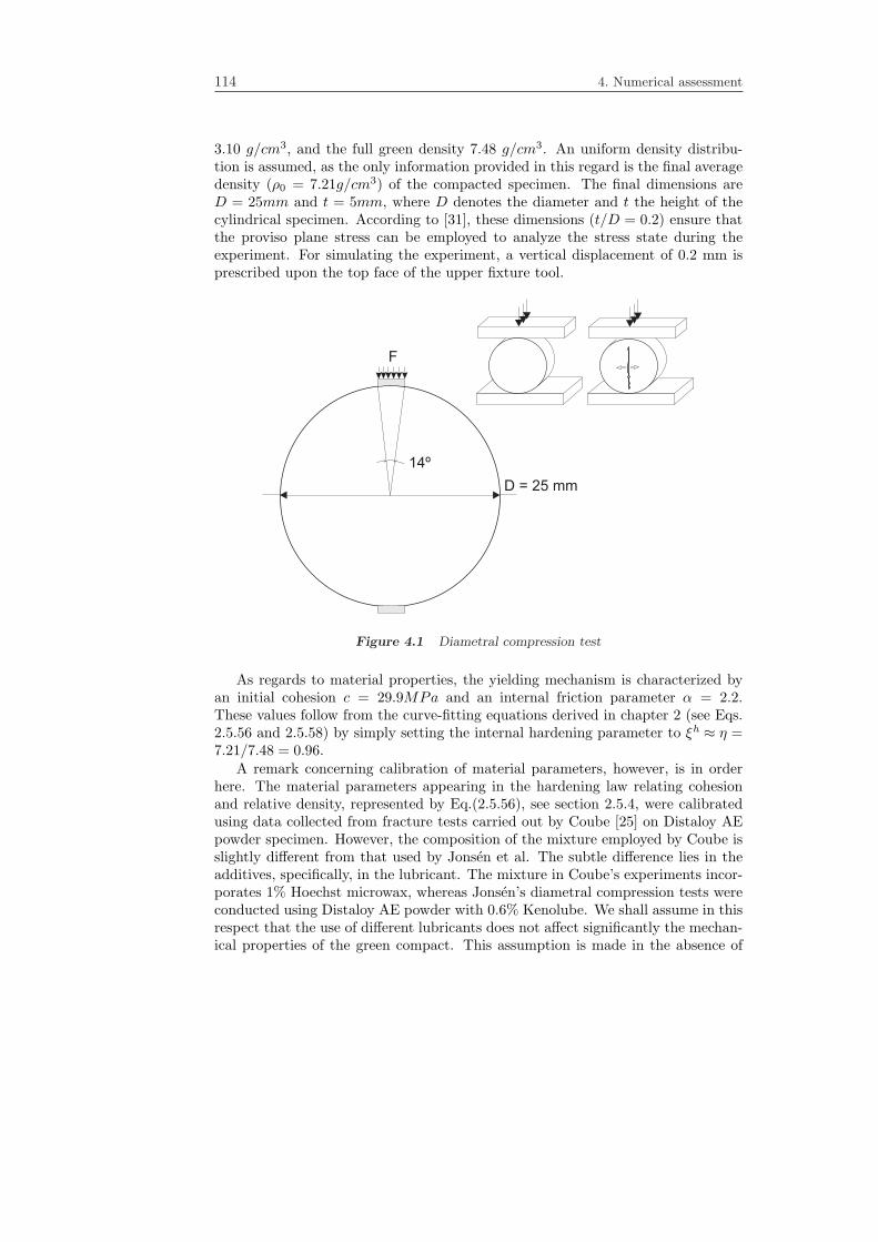
114 4. Numerical assessment
3.10 g/cm3, and the full green density 7.48 g/cm3. An uniform density distribu-tion is assumed, as the only information provided in this regard is the final averagedensity (ρ0 = 7.21g/cm3) of the compacted specimen. The final dimensions areD = 25mm and t = 5mm, where D denotes the diameter and t the height of thecylindrical specimen. According to [31], these dimensions (t/D = 0.2) ensure thatthe proviso plane stress can be employed to analyze the stress state during theexperiment. For simulating the experiment, a vertical displacement of 0.2 mm isprescribed upon the top face of the upper fixture tool.
F
D = 25 mm
14º
Figure 4.1 Diametral compression test
As regards to material properties, the yielding mechanism is characterized byan initial cohesion c = 29.9MPa and an internal friction parameter α = 2.2.These values follow from the curve-fitting equations derived in chapter 2 (see Eqs.2.5.56 and 2.5.58) by simply setting the internal hardening parameter to ξh ≈ η =7.21/7.48 = 0.96.
A remark concerning calibration of material parameters, however, is in orderhere. The material parameters appearing in the hardening law relating cohesionand relative density, represented by Eq.(2.5.56), see section 2.5.4, were calibratedusing data collected from fracture tests carried out by Coube [25] on Distaloy AEpowder specimen. However, the composition of the mixture employed by Coube isslightly different from that used by Jonsen et al. The subtle difference lies in theadditives, specifically, in the lubricant. The mixture in Coube’s experiments incor-porates 1% Hoechst microwax, whereas Jonsen’s diametral compression tests wereconducted using Distaloy AE powder with 0.6% Kenolube. We shall assume in thisrespect that the use of different lubricants does not affect significantly the mechan-ical properties of the green compact. This assumption is made in the absence of

4.2 Diametral compression test 115
experimental data concerning cohesion of Distaloy AE with 0.6% Kenolube. Nev-ertheless, we must note carefully that presuming that the cohesion (green strength)of a green compact part is not influenced by the type of lubricant and the additionlevel is quite objectionable, as it is shown in the work of Degnan et al. [29], and,therefore, this hypothesis should be adequately contrasted in future developments.
As mentioned in previous chapters, the characterization of the elastic responseis a somewhat controversial issue. Two empirical relations were presented in section2.5.4 for the Young’s modulus as a function of relative density (internal hardeningvariable) (see Eqs. 2.5.60 and 2.5.61). Evaluation of the former, the one advocatedby Pavier [83], at ξh = 0.96 yields Ee = 168444.0MPa, whereas the linear relationproposed by Coube [25], on the basis of measurements of the velocity of sound onan unstressed specimen Eq.(2.5.61), gives Ee = 21127.0MPa. The consequencesof using one or the other relation will be properly assessed later. Other relevantmaterial parameters are the Poisson’s coefficient (νe = 0.29) and the intrinsicsoftening modulus, which can be obtained from the graph shown in figure 2.23,giving H0 = 9.0 · 105MPa/mm. The dilatancy factor γ is set to 0.01.
4.2.1 Results
4.2.1.1 Numerical aspects
Prior to compare the experimental results with the calculated response, it is expe-dient to carry out a preliminary convergence analysis, under refinement of the dis-cretized time and spatial domains, and to investigate the implications of employingeither standard displacement-based or mixed displacement-pressure formulations.The experimental data that will serve as the basis for the quantitative assessmentof the problem is the graph of applied load F versus deflection v in the verticaldirection. Thus, it seems appropriate to perform these analysis by examining F −vplots. The vertical deflection v corresponds to the displacement prescribed uponthe nodes located at the top face of the fixture tool, whereas the applied load F isobtained as the sum of the forces at these nodes.
Using the mesh layout displayed in figure 4.2, in which the higher mesh densityin the vertical central band is dictated by foresight of the fact that the dominantcrack will be located along the loaded diameter, and setting Ee = 21127.0MPa,a study varying the number of time steps3 is undertaken. Figure 4.3 shows theresult of such study. The plot of applied load versus deflection takes essentiallythe same form in all the studied cases, the only substantial difference being thepost-peak behavior. The branch OA corresponds to linear elasticity. After pointA, a slight decrease in slope occurs. This subtle change of stiffness indicates crackinitiation at the center of the disc. The development of the central dominant crackprogresses until the maximum force is reached (point B in case N = 800). Themagnitude of the maximum force estimated using N = 50 steps differs from that
3In order to facilitate the comparison, equally space intervals have been used. However, weshould note that considerable gain in computational efficiency can be achieved by means of anadaptive time stepping scheme, as the one proposed by Oliver et al. [79]. For instance, due tothe implicit contribution of the IMPLEX integration algorithm, the elastic response OA could beobtained in a single step.

116 4. Numerical assessment
Figure 4.2 Mesh layout
0 0.02 0.04 0.06 0.08 0.1 0.12 0.14 0.16 0.18 0.20
1
2
3
4
5
displacement (mm)
Applie
d forc
e (k
N)
n =800
n =400
n =200n =100
n = 50
A
B
C
D
Figure 4.3 Applied load versus deflection. Results for several number of time steps.
calculated with N = 800 by only 4.3 %. Following the attainment of the peak-load, the central fiber suddenly ceases to contribute to the rigidity in the verticaldirection, and the computed force drops rapidly (point C). The abruptness of thisdecay is accentuated as the time step size is reduced. The post-peak ascendingbranch (CD) corresponds, approximately, to the response of a specimen spli intotwo halves. As it is apparent that further increase in the number of step willnot significantly improve the accuracy, the prediction using N=800 steps will beconsidered as reliable, and therefore, this discretization of the time domain will be

4.2 Diametral compression test 117
employed throughout the subsequent simulations. It has to be mentioned that, incomputing the five cases presented, only one equilibrium iteration at each time stepwas required to achieve convergence.
Displacement (mm)
0 0.02 0.04 0.06 0.08 0.1 0.12 0.14 0.16 0.18 0.20
1
2
3
4
5
6
Ap
plie
d lo
ad
(kN
)
h=0.8 mm
h=0.4 mm h=0.6 mm
h=1 mmh=2 mm
Figure 4.4 Applied load against deflection. Result for several meshes, characterized bythe size h of their elements.
Our concern now is to examine the sensitivity of the numerical results to sub-sequent mesh refinement. Five different meshes characterized by the size of theirelements h are used4. Computed results are shown in figure 4.4. As far as themagnitude of the peak value of the load is concerned, the sequence of graphs dis-played in figure 4.4 exhibits clear convergence with refinement of the mesh. Thepeak value predicted by using the mesh labelled as h = 0.4mm is only a 0.6 %lower than the one obtained with the coarser mesh h = 0.6mm. On the otherhand, the magnitude of the “residual force” - the force calculated at the onset ofthe post-peak ascending branch - ranges between 2.85 kN and 2.91 kN, althoughwithout a clear monotonic convergence tendency. In view of these circumstances, itseems that going to finer discretizations will not improve significantly the accuracy.Hence, the mesh labelled as h = 0.4mm, which corresponds to the one displayedpreviously in figure 4.2, will be taken as the finite element mesh for the simulationsshown in the sequel.
The force versus displacement curves obtained by using two different finite ele-ment procedures, namely, a standard displacement-based formulation and a mixeddisplacement-pressure approximation, are depicted in figure 4.5. Inspection of thisdiagram indicates that the use of one or another formulation is inconsequential, asthe two curves are practically indistinguishable.
4The mesh layouts used in this study are patterned after the non-uniform mesh depicted infigure 4.2. The typical size h corresponds hence to the size of the elements in the central regionthat will eventually contain the dominant crack. Care is to be exercised in selecting the mesh sizein the region where the load is applied to the specimen, since excessively coarse meshes may notrepresent adequately the stress concentration, leading to a mechanism of failure different fromthat of cracking along the loaded diameter.

118 4. Numerical assessment
Displacement (mm)
App
lied lo
ad
(kN
)
Standard formulation
Mixed formulation
0 0.02 0.04 0.06 0.08 0.1 0.12 0.14 0.16 0.18 0.20
1
2
3
4
5
Figure 4.5 Applied load against deflection. Comparison between results computedusing a standard displacement-based formulation and a mixed displacement-pressure for-mulation.
Displacement (mm)
Applie
d load (
kN
)
0 0.04 0.08 0.12
A
M
NP
QS
B
B
C
C
D
0.16 0.20
1
2
3
4
5
6
Numerical result (
Numerical result ( Mpa)Experimental (Jonsén et al.)
= 21127.0 MPa)e
E
= 168444.0e
E
2.00.156 0.158 0.160
2.5
3.0
3.5
4.0
4.5
5.0
Figure 4.6 Applied load versus deflection. Comparison of computed results using dif-ferent elastic properties with experimental data collected by Jonsen et al. [49]. Thepost-peak descending branch B-C is shown in magnified form.
4.2.1.2 Computed versus experimental results
Quantitative results
We are now in the position to compare the computed response (using N =800 steps , typical mesh size h = 0.4mm and standard displacement-based for-mulation) with the experimental results. The plots of the computed force ver-sus vertical deflection for two distinct Young’s modulus Ee = 168444.0MPa andEe = 21127.0MPa, in conjunction with the corresponding experimental curve, pro-

4.2 Diametral compression test 119
vided by Jonsen et al. [49], are depicted in figure 4.6. This diagram clearly showsthat the Young’s modulus estimation Ee = 168444.0MPa, obtained from triaxialmeasurements [83], is utterly inadequate for characterizing the elastic response ofthe green compact under the conditions of this diametral compression test, beingmore appropriate the estimation Ee = 21127.0MPa, derived from ultrasound tests[25]. Nonetheless, even in this case, significant differences with experimental dataare observed. Indeed, the slope of the numerical F − v graph remains constantuntil point A. By contrast, the plot of the experimental force versus deflectiontraces initially a non-linear path OM. Then, it becomes linear up to the point N,at which, according to Jonsen et al. [49], the elastic nature of the graph ceasesdue to the initiation of the central crack. The progressive decrease in slope ob-served experimentally (path NP) during crack growth is more pronounced that thedecrease in slope predicted by the model (path AB), which is practically unnotice-able. As a consequence, the computed peak load (point B) exceeds notably (20 %)the maximum force measured experimentally (point P). Discrepancies in the post-peak behavior are also noteworthy. In the experiment, a relatively gradual decay ofload is recorded (path PQ), whereas this decay occurs precipitously (path BC) inthe simulated response, resulting a residual force underestimated by approximately30 %. The enlarged view of path BC, shown in the upper-right part of figure 4.6,reveals that the transition from B to C, albeit quite abrupt, is not instantaneous,that is, several time steps are required in its computation5.
Qualitative results
Figure 4.7.a contains images recorded experimentally by Jonsen et al [50] duringthe loading process. The leftmost picture corresponds to the initiation of the crackat the center of the disc (point N in the F − v curve shown in figure 4.6). Thecentral image shows the state of the crack at the point of maximum load (pointP in figure 4.6). Finally, the rightmost picture displays the aspect of the crackat the end of the loading process (point S in figure 4.6). Aside from the central“dominant” crack, secondary cracks are distinguishable around the contact zones.
Cracks impair strength. Thus, a natural way of representing such defects isby plotting contours of cohesion (green strength), in which crack locations areidentified as those areas affected by a local decrease of cohesion. The correspondingsequence (initiation of the central crack, maximum load and end of the test) ofcomputed contour plots of cohesion is shown in figure 4.7.b. In the leftmost plot,the local decay of cohesion observed in the center of the disc indicates the initiationof the crack. In the central contour plot (maximum load), we can see that this loss ofcohesion propagates to the periphery of the disc along the loaded diameter. Close tothe center of the disc, this propagation occurs along a single path. Near the loadingsurface, however, the de-cohesion path seems to bifurcate into two branches. Suchbifurcation (or “crack branching”) is not detected in the experiment. Inspection ofthe rightmost plot (end of the test), indicates that, eventually, loss of cohesion hasbeen more intense along one of these branches. The resulting “dominant” path,
5An instantaneous drop would correspond to a perfectly brittle response. A force versus dis-placement graph that exhibits such feature warns of trouble with potential snap-back behavior [27].

120 4. Numerical assessment
(a)
(b)
( c )
29.5
Cohesion (Mpa)
3.69
7.37
0
11.06
14.75
18.44
25.82
22.12
Figure 4.7 (a) Images recorded experimentally by Jonsen et al [50]: initiation of thecrack, point of maximum load, and end of the loading process. (b) Contour plots ofcomputed cohesion corresponding to such stages. (c) Contour plot of computed cohesionat the end of the loading process, showing the spatial grid used in the computation.
which spans approximately 80% of the length of the diameter, displays a distinctly

4.2 Diametral compression test 121
crack-like appearance, and bears close similarity with the crack observed in thecorresponding photograph. Note that other regions with relatively low cohesion,located mainly around the contact zones, are discernable in the final contour plot.The aspect of these patterns of low cohesion are in remarkable agreement with theabovementioned secondary cracks detected experimentally.
mm
Horizonta
l dis
pla
cem
ent (m
m)
Horiz disp. (mm)
0.06
-0.06
0.047
0.03
0.02
-0.02
-0.03
-0.047
0.001
-0.001
0 5 10 15 20 25-0.062
-0.037
-0.012
0.013
0.038
0.06
M
M
M’
M’
A A’
Figure 4.8 Horizontal displacement contour lines. The graph shows the horizontal
displacement measured along the horizontal diameter AAA´.
In figure 4.7.c, the final cohesion contour is plotted in conjunction with the fi-nite element mesh used for the computation. This plot allows us to distinguish theband of elements along which loss of strength is localized. A result that also assistsin visualizing this localization phenomenon is the plot of horizontal displacementcontour lines, displayed in figure 4.8. Close spacing of lines relates to steep slopesand wide spacing to gentle inclines. Hence, the intense concentration of lines pre-sented along the loaded diameter is indicative of an abrupt change in the horizontaldisplacement, as it is shown in the accompanying graph of figure 4.8.

122 4. Numerical assessment
4.2.2 Discussion and concussions
The numerical results shown in figure 4.3 serve as a convincing proof that the solu-tion provided by the IMPLEX integration algorithm converges as the length of thetime step is reduced. In addition, we pointed out that only one iteration per step,for the five cases presented, was required to achieve convergence to equilibriumstates, a fact that highlights the robustness of the IMPLEX integration scheme.Not least among its merits is the ability to compute the post-peak response (curveBCD in figure 4.3). A pure implicit integration scheme, without further enhance-ments such as cumbersome continuation methods [71, 27], would probably fail insimulating the post-peak behavior, since the tangent stiffness matrix derived fromthis integration scheme ceases to be positive definite at this point.
The sequence of force versus displacement diagrams presented in figure 4.4 indi-cates that the energy6 dissipated during the loading process apparently convergesas the mesh is refined. As mentioned in section 2.1.2.1, lack of convergence upon re-finement of the finite mesh is one of the flaws that plagues the numerical treatmentof models exhibiting strain-softening behavior. Hence, the proposed regularizationof the softening law proves useful, at least in this example, in alleviating this prob-lem. We should note that this assessment only furnishes information regardingthe dependency of the results on the size of the elements. A complete assessmentshould also acknowledge the directional dependence on mesh topology [4]. Thesmeared crack model presented in this work is very elementary in this respect anddoes not contain any enhancement to deal with such issue . The predictions madeby our model will be thus inevitably affected by this mesh-induced directional bias.However, knowing with detail the exact orientation of the potentially developingcracks is not the goal of our analysis, thus such modeling deficiency is relativelyinconsequential.
It is widely known that, in many applications such as metal plasticity, the useof linear triangular elements in conjunction with displacement-based finite elementformulation, suffers a detrimental overstiff phenomenon known as “volumetric lock-ing” [9]. With a view towards assessing the efficiency, in our context, of the standardformulation in comparison with alternative formulations not theoretically prone tovolumetric locking, a mixed finite element approximation with displacements andpressure as basic variables has been tested. Results presented in figure 4.5 wereaimed at comparing the calculated force versus displacement response under thesetwo approaches. According to this diagram, no appreciable differences are foundin using mixed or standard formulation. This “unexpected” similarity may be ex-plained as follows. The developing of the crack (see figure 4.7) along the loadeddiameter takes place under mode I or opening mode conditions, which, inciden-tally, are the same conditions that characterizes fracture in a pure tensile test. Thisimplies that the the stress state at a representative plastically deforming elementtraces a path which lies approximately within the first quadrant of the p-q plane
6Recall (see figure 2.21) that the energy dissipated can be estimated in terms of the areaenclosed by the force displacement graphs of unsplitted and splitted tests.

4.2 Diametral compression test 123
(tensile regime). As illustrated in figure 2.9 (chapter 2), in this stress regime, theplastic flow involves a dilatational component, due to the use of a parabolic plasticpotential function, and this volumetric component, in turn, becomes dominant asthe stress state approaches the vertex of the Drucker-Prager failure line. Hence, thematerial represented by our plasticity model in this range of stresses is not plasti-cally incompressible. The absence of this kinematical constraint may thus explainwhy both formulations yield identical responses7.
According to the preceding discussion, thus, the simulation of cracks whichdevelops under mode I is not affected by volumetric locking, even when usingstandard displacement based formulation. Experimental observations indicate that,during the manufacturing process, the vast majority of cracks usually grows underthis opening mode [99]. Consequently, in view of these facts, and considering,in regards to the mixed approach, the increase of computational effort and thepreviously mentioned questionable reliability of the stabilization procedure, it seemsreasonable to favor the standard displacement based formulation over the mixedapproach. Certainly, volumetric locking may emerge in other situations. At highdensities, for instance, the material flows at constant volume when yielding onthe von Mises yield surface, i.e., it becomes plastically incompressible. However,as mentioned in chapter 2, the validity of the constitutive relationships might bequestionable as a whole, since the basic hypothesis of small elastic strain is violated.Hence, further sophistication is not warranted.
As regards the results shown in figure 4.6, the large difference observed be-tween the responses obtained by using different elastic parameters conveys therelevance of choosing an adequate estimation for the Young’s Modulus. In thiscase, the computed F −v graph corresponding to the the Young’s modulus estima-tion Ee = 21127.0MPa, derived from ultrasound tests conducted by Coube [25],is in closer agreement with the experimental data. This fact is in conformity withthe argument set out in section 2.5.4 when dealing with the calibration of the elas-tic parameters, according to which, Coube’s empirical relationship (Eq.(2.5.61)) ismore appropriate in circumstances of low degree of confinement. However, even inthis case, significant discrepancies between predicted and experimental curves aredetected.
The different elastic behavior exhibited by the computed response and the expe-rimental data, linear and non-linear8, respectively, highlights, again, concern withthe characterization of the elastic response, which should receive more careful con-sideration in future improvements of the model. On the other hand, the differenttrends observed in the inelastic branches up to the peak load -the computed re-sponse has a steeper slope (see figure 4.6, paths AB)- may be attributable to several
7Another apparently plausible explanation is that, in plane stress problems, the thickness ofthe element can change to accommodate incompressible materials, and hence volumetric lockingwill not occur[5]. However, as alluded to earlier, this reasoning is not valid, as the plane stressproviso is imposed here in an approximated manner, which follows from a plane strain formulationby an appropriate conversion of elastic constants.
8The non-linear behavior at the beginning of the curve may be alternatively attributed toinitial seating and settling errors during experiments, and not necessarily to non-linear materialbehavior.

124 4. Numerical assessment
factors. A plausible explanation is that the stress conditions along the localizationband may be not adequately represented by the approximated plane stress formu-lation. This hypothesis should be corroborated in future developments by under-taking a three-dimensional analysis. The model overpredicts the maximum forcein approximately 20 %, and the displacement at which this peak value is reachedin 11 %., amounts which are within a reasonable range of accuracy, consideringthe significant uncertainty (10-15%) attached to the experimental determination oftensile properties in green compacts9.
The post-peak portion of the curve corresponds to the unstable growth of thecentral dominant crack. The computed force experiments a drastic decrease, as op-posed to the relatively mild decay observed experimentally. The computed residualforce is underestimated in approximately 30%. As a result, the energy dissipatedduring the process is overestimated. The main contributor to this discrepancy10
may be found in the elementary character of our crack modeling approach. Indeed,as mentioned earlier, our model does not permit a precise tracking of the developingcracks. As a consequence, the propagating localization band could tend to followcertain preferred directions dictated by the mesh, and, eventually it may travelalong bifurcated paths, giving rise to spurious “crack branching”, as the one ob-served in the contour plot of cohesion displayed in figure 4.7.b (central picture). Animmediate implication of such spurious branching is that the extent of the regionaffected by loss of cohesion increases, resulting in a overestimation of the dissipatedenergy.
We reiterate that the quality of the obtained results must be judged in the lightof the aim and purpose of our investigation. The model has undoubtedly proved tobe efficient in detecting the formation of the experimentally observed macroscopiccrack. In addition, as seen in figure 4.7, the de-cohesion pattern predicted bythe model is in remarkable agreement with the experimental images of the crackdevelopment. Admittedly, the results can be improved. However, as it may beinferred from the preceding discussion, if one wishes to bring the computed solutioninto closer agreement with experimental evidence, aside from possible refinementsof the hypothesis involved in the calibration of the fracture energy, it would benecessary to abandon the elementary smeared crack approach in favor of moresophisticated, and complex, continuum-based methods [75].
9The material parameter that has more influence in the location of the peak load is the cohesionvariable (c). Note that the experimental values for cohesion shown in chapter 2 are derived data[14], in the sense that they are obtained from raw data (tensile and compression strength, forinstance) through an interpretation process full of assumptions. Thus, in addition to the errorinvolved in obtaining the raw data, one has to acknowledge the uncertainty associated to suchassumptions.
10The post-peak portion of the curve is also highly sensitive to test conditions [61]. Hence,the relevant features of the experimental environment (total stiffness of the testing frame, forinstance) should be also acknowledged if the response is to be accurately predicted.

4.3 Pressing and ejection of a thin cylindrical part 125
4.3 Pressing and ejection of a thin cylindrical part
A cylindrical part made of an iron based Distaloy AE powder, with apparent densityρapp = ρ0 = 3.04 g/cm3 and theoretical density ρth = 7.33 g/cm3 is pressed untilreaching a final density ρ = 7.18g/cm3. The punches and the die are consideredelastic materials characterized by a Young’s modulus Etool = 210000MPa and aPoisson’s ratio νtool = 0.3. Their dimensions are displayed in figure 4.9.
Die
Upperpunch
R = 25 mm
h = 140 mm
Lowerpunch
1
up
h
= 2
38
mm
lph
= 1
5.1
2 m
m0
R = 85 mm2
Powder
Figure 4.9 Dimensions of punches and initial die cavity.
The motion of the upper and lower punches is controlled by prescribing verticaldisplacements on its top and bottom surfaces, respectively. During pressing, theupper punch moves downward with constant velocity 10mm/s while the lowerpunch and the die remain stationary. Release of axial pressure takes place at a rate20mm/s by gradually lifting the upper punch. During ejection from the die, thelower punch pushes the compact upward at a constant rate 40mm/s.
This example focuses on the formation of cracks due exclusively to elastic ex-pansion of the compact upon exiting the die. Contribution of friction effects to theoccurrence of cracks will be therefore ignored by setting the friction coefficient toa low constant value 11 µ = 0.01. Furthermore, these circumstances of negligiblefriction will allow us to draw approximated analytical expressions for estimatingthe stress state during axial unloading. In order not to disrupt the continuity ofthe presentation, these derivations are relegated to appendix B.3.
Material parameters are obtained from the calibration presented in chapter 2.
11Assuming an ideally frictionless process is not advisable since, upon total removal of the upperpunch, ill-conditioning may arise due to the absence of restrictions on the vertical direction.

126 4. Numerical assessment
We recall that two alternative empirical relationships for the Young’s modulus as afunction of relative density were quoted. Here we shall adopt the one advocated byPavier [83], see Eq.(2.5.60), since it yields substantially larger values that Coube’sestimation [26] (see Eq.(2.5.60)) and, therefore, the effects of elastic expansion areaccentuated.
Figure 4.10 Initial mesh layout.
The initial finite element mesh is shown in figure 4.10. The average size of theelements of the powder body is le = 1mm, whereas the size of the elements atthe boundaries of punches and die in contact with the powder is, approximately,0.5mm. In general, a practice that proves advantageous in ensuring a successfulperformance of the contact-detection algorithm is to select the element size at theboundaries of the tooling bodies equal or smaller than the element size used atthe boundary of the powder body. Tooling elements can be graded from small-sizeat the boundaries in contact with the powder to become coarser with increasingdistance from these surfaces.
4.3.1 Results and discussion
4.3.1.1 Study of convergence with refinement of time discretization
In the example of the Brazilian test, see section 4.2.1.1, the issue of convergenceunder refinement of the time discretization was examined in a problem involvingsoftening behavior. The goal now is to explore this issue in situations in whichhardening behavior dominates the response, i.e., during pressing of the powderwithin the die.

4.3 Pressing and ejection of a thin cylindrical part 127
Axia
l p
ressu
re (
Mp
a) n = 10
n = 50
n = 100
n = 200
AA
Time (s)
0 0.1 0.2 0.3 0.4 0.5 0.6 0.7 0.8 0.9 10
100
200
300
400
500
600
700
0.92 0.94 0.96 0.98 1400
450
500
550
600
650B
B
Figure 4.11 Average axial pressure during pressing versus time. Results for severalnumber of time steps (uniformly spaced). The final portion of the curves is shown inmagnified form.
Figure 4.11 shows axial pressure versus time graphs computed using differentnumber of (constant) time steps. The sequence of graphs is clearly convergent.The simulation with N = 200 steps can be taken as the “correct” solution, as it isapparent that going to smaller time step sizes will not improve significantly the ac-curacy of the predictions. Inspection of the initial portion of the curves, however,reveals an anomalous behavior. At the very first increment, the solution calcu-lated for the four cases presented “overshoots”. The magnitude of the deviationdecreases as the time step is reduced, being practically imperceptible for N = 200steps. This overshooting is not connected with any type of instability, since thecomputed response returns to the presumably correct course at the second step.For instance, for N = 50 steps, the axial stress computed at the first incrementis largely overestimated (40 MPa, in contrast to the 0.1 MPa predicted with N =200 steps). Despite this initial substantial error, the drift from the correct curvein subsequent increments remains bounded, being the magnitude of the maximumpressure (compaction pressure) only 3.5 % below the pressure computed with N =200 steps.
The origin of this non-physical overshooting behavior is to be sought in the nu-merical integration of the constitutive equation, more precisely, in the intricacies ofthe IMPLEX integration scheme. As explained in section 3.1.1, the essence of thisintegration procedure is to obtain the stresses and other state variables at a giventime step in terms of variables computed at the previous time step by accomplish-ing an implicit integration. At the very first increment, obviously, no informationis available to carry out the extrapolation. The integration algorithm resolves this

128 4. Numerical assessment
n = 200 equally-sized time steps
n = 50 variable-sized time stepn = 50 equally-sized time steps
Axia
l p
ressu
re (
Mp
a)
Time (s)
0 0.1 0.2 0.3 0.4 0.5 0.6 0.7 0.8 0.9 10
100
200
300
400
500
600
700
B
0.92 0.94 0.96 0.98 1400
A
450
500
550
600
650
A B
Figure 4.12 Average axial pressure during pressing versus time. Results for severalnumber of time steps (constant and variable time steps). The final portion of the curvesis shown in magnified form.
inconsistency by further assuming that the plastic multipliers are initially zero.Such assumption, in turn, amounts to presume that the body behaves elasticallyat the first step. This explains why, for the four cases, axial stresses at the firstincrement lie along a straight line (see figure 4.11).
It follows then that the natural way to counteract this overshooting problemis to reduce the time step size12. However, dimishing uniformly the step size overthe whole time domain is not an efficient practice. It is preferable a “smart”distribution of the time step lenght that permits the reduction of the integrationerror at reduced computational cost. To reinforce this view, in figure 4.12, theresponse obtained using 50 and 200 equally-sized spaced time intervals is comparedwith the solution computed with 50 variable-sized time steps. The size distributionfor the non-uniform discretization is shown in figure 4.13.b. The relatively smallsize of the two first intervals is dictated by the need to overcome the overshootingproblem. The size of the subsequent time steps is directly connected with thecompressibility of the material. As the slope of the pressure versus density curvebecomes more pronounced, the length of the time step is progressively reduced, sothat the incremental changes in stress remains approximately constant. Inspectionof figure 4.12 indicates that a similar level of accuracy is obtained by using either
12Alternative ad-hoc procedures can be put forward to alleviate this problem. For instance, aplausible option is to obtain the response at the initial step by performing a classical pure implicitintegration. This procedure is quite effective provided the exact implicit algorithmic tangentmoduli is available. Such not being the case, convergence failure may occur and, therefore, thesolution may be “worse than the disease”.

4.3 Pressing and ejection of a thin cylindrical part 129
0 10 20 30 40 500
0.02
0.04
0.06
0.08
0.1
0.12
0.14
0.16
0.18
Time stepTime step
(a)Le
ngth
of t
he ti
me
inte
rval
(s)
Itera
tions
per
tim
e st
ep
0 10 20 30 40 500
1
2
3
4
(b)
Figure 4.13 (a) Number of iterations (global scheme) against time step number and(b) length of the time interval versus time step number. Both results correspond to thecase N = 50 (variable) steps shown in figure 4.12
200 steps uniformly spaced or 50 steps with sizes non-uniformly distributed. Theuse of this “smart” step size distribution has reduced thus the computational effortby a factor 200/50 = 4. Finally, figure 4.13.b. displays the number of globalequilibrium iterations required to achieve convergence at each increment for thecase N = 50 variable time steps. The number of iterations ranges between 2 and 4,resulting in a total number of computational cycles (number of increments timesnumber of iterations) of 113.
4.3.1.2 Assessment of the contact algorithm
Figure 4.14 displays the average axial and radial pressure versus time on the com-pact during pressing and axial unloading computed with two different contact al-gorithms, namely, the contact penalty method and the augmented Lagrangian tech-nique13. The penalty factor, denoted here as Kp, is made proportional to theYoung’s modulus14 of the material, that is, Kp = aEe. Two values of the propor-tionality factor a has been tested.
The initial shallow portion of the curves is not shown, since the three solutionsare practically identical. The ascending and descending branches correspond to
13The augmented Lagrangian method is applied together with a double loop Uszawa type al-gorithm.The inner loop refers to the iterations for solving the weak form whilst the lagrangemultiplier is held constant. The outer loop serves for updating the lagrange multiplier [110].
14As mentioned at the outset of this chapter, the contact detection algorithm used here is basedon the construction of an powder-tooling interface mesh[77]. This, in turn, allows us to define thepenalty parameter locally at each element of the interface mesh. Here it is made proportional tothe Young’s modulus of the powder elements adjoining the nodes that define the correspondinginterface element.

130 4. Numerical assessment
0.750.7 0.8 0.85 0.9 0.95 1 1.050
100
200
300
400
500
600
700
Radial
Axial
Time (s)
Pre
ssure
(Mpa)
Augmented lagrangian
pPenalty, K = 10 Ee-2
pPenalty, K = 10 Ee-1
PressingAxial loadrelease
rs
zs
zs
rs
zsmax
rsmax
rsres
Figure 4.14 Average axial and radial pressure versus time (during pressing and axialload release stages). Comparison between results computed by using two different con-tact algorithms, namely, a contact penalty strategy, for two different penalty parametersKp (which are proportional to Young’s modulus Ee of the compacting powder), and anaugmented lagrangian technique.
pressing and axial unloading, respectively. The penalty method with the largerparameter (a = 10−1) and the augmented lagrangian technique are undistinguish-able up to t = 0.92 s for both axial and radial pressures. Thereafter, the penaltysolution with larger parameter (a = 10−1) oscillates about the smooth solution ob-tained with the augmented lagrangian method. The oscillations are more intense inthe axial response. The response calculated with the low penalty factor (a = 10−2)exhibits a progressive drift from the other two solutions. The magnitude of thisdeviation at the end of pressing is approximately 10 % for both axial and radialpressures, whereas the radial pressure upon total axial unloading, denoted by σresr ,is underestimated by almost 12 %.
The solution obtained by using the augmented Lagrangian strategy can be con-sidered as the more accurate, and therefore reliable, solution, since the constraint ofimpenetrability is more rigorously enforced that in the penalty case, at the expense

4.3 Pressing and ejection of a thin cylindrical part 131
Time (s)
0.85 0.9 0.95 1 1.05
0
100
200
300
400
500
600
700
Augmented lagrangian
pPenalty, K = 10 Ee-2
pPenalty, K = 10 Ee-1
zs
Axia
l str
ess, -
(Mpa)
zs
Figure 4.15 Axial stress, at a node located on the top surface of the compact, versustime (pressing and axial load release stages). Comparison of the performance of penaltyand augmented lagrangian contact techniques.
of a substantial increase of computational cost 15. The gradual deviation of thepenalty solution with the low parameter (a = 10−2) is due precisely to a poor en-forcement of the non-penetration constraint. On the other hand, the non-physicaloscillatory behavior exhibited by the penalty response with the large parametera = 10−1 can be plausibly attributed to an ill-conditioning of the problem dueto an excessive large penalty factor. The magnitude of such oscillations becomesmore evident by plotting, instead of average pressure, the axial stress at a nodebelonging to the upper boundary surface (see figure 4.15).
If the scope of the analysis were to merely examine average density and stressesafter compaction in relatively large domains, the effect of these oscillations wouldbe not too deleterious. Indeed, during the analysis of the pressing stage, this oscil-latory behavior manifests itself in uneven density and stress distributions along theboundary of the powder body. Due to the stable character of hardening behavior,these uneven patterns tend to dissapear as we move far from the boundary, andas a consequence, final average quantities are not seriously affected. By contrast,the consequences of inaccurately resolving the contact response are more dramaticwhen the main concern is the analysis of cracks. The reason behind this is thesensitiveness, of both physical and computational nature, exhibited by the greencompact during the post-pressing operations. If the oscillations of the computed
15For the outer loop, the number of iterations is between 4 and 20, on average 8, dependingon the difficulty in determining the correct status (active or inactive) of the interface elements.This implies that the computational cost rises more than 8 times in comparison with the moresimplistic contact penalty approach.

132 4. Numerical assessment
forces are sufficiently severe, the stress state at a boundary element may resultseriously perturbed, with the consequent drop of mechanical strength (cohesion).Due to the unstable nature of softening materials, this perturbation may propageinwards, leading to the formation of “spurious” numerical cracks, which can bequite misleading and eventually lead to incorrect design decisions.
In view of the importance of obtaining an oscillation-free contact response, theaugmented Lagrangean contact strategy appears to be more appropriate. Thesolution with the small penalty parameter a = 10−2 is also ostensibly smoothand regular, and, in addition, the maximum deviation in predicting final forcesis approximately 12%, which, although certainly not a negligible error, can beconsidered within acceptable engineering accuracy. However, we should keep inmind that the choice of this particular penalty factor is based on heuristics ratherthan in any physical argument. Although it gives an oscillation-free response inthis example, it is uncertain whether it will behave satisfactorily in other cases.Therefore, in the interest of robustness and reliability of the computed solution,it is preferable to adopt the more expensive augmented Lagrangian strategy forcomputing, at least, the contact response during the phases of axial pressure releaseand ejection from the die.
Analytical estimation of the lateral pressure upon axial unloading
The residual radial pressure, denoted as σresr , is the pressure exerted by thedie upon total release of the applied axial load (see figure 4.14). This pressureand the roughness of the die wall will determine the magnitude of the frictionalforces that will have to be overcome for ejecting the part. According to the radialpressure versus time graph shown in figure 4.14, the residual lateral pressure, forthe augmented Lagrangean case , yields |σresr | ≈ 320MPa. Considering that themaximum radial pressure is |(|σmaxr ) ≈ 517MPa, this implies a reduction in lateralpressure of 38% upon axial unloading.
In appendix B.3, the stress state during axial load release is studied analyticallyby presuming elastic conditions and a homogeneous deformation state. Accordingto Eq.(B.3.9) in this appendix, such drop in lateral pressure can be expressed as afunction of the compaction pressure |σmaxz |:
|∆σr| = Mul|σmaxz |, (4.3.1)
where Mul is a parameter that includes the effects of the die geometry and theelasticity of the powder and the die:
Mul =νe
(1− νe) +Ee
Ktool
. (4.3.2)
The Young’s Modulus of the powder Ee can be obtained by evaluating expres-sion Eq.(2.5.60) (section 2.5.4) at ξh ≈ η = 7.18/7.33 = 0.98, yielding Ee =196068MPa. The constant Ktool represents the stiffness of the die in the ra-dial direction (see figure B.3 in appendix B.3). For the given geometry Ktool =470600MPa. Substituting these quantities in Eq.(4.3.2), we have Mul = 0.28.

4.3 Pressing and ejection of a thin cylindrical part 133
Thus, taking into account that |σmaxz | ≈ 685MPa, the drop in lateral pressureestimated analytically gives 37%, only 1% less than the decrease calculated withthe finite element solution.
4.3.1.3 Assessment of the crack prediction methodology
We consider first the case corresponding to an ejection with total removal of theupper punch followed by an upward movement of the lower punch. Figure 4.16.acontains a sequence of three contour plots of cohesion during this ejection process.In the leftmost plot, the compact is still confined within the die cavity. It followsfrom the uniformity exhibited by the cohesion distribution that the green strengthhas not been altered and remains at the same value attained at the end of thepressing stage. In the central plot, almost one half of the compact has alreadyemerged from the die. To make more distinguishable changes in cohesion, thisplot is displayed in magnified form in figure 4.16.b with a narrower grayscale. Ade-cohesion pattern, in the form of darker “spots”, is observed along the emergedportion of lateral surface. This mechanical damage is apparently superficial, sinceonly the outer layer of elements is appreciably affected by loss of cohesion.
The rightmost plot of figure 4.16.a is the cohesion contour map at a point where85% of the upper portion of the part is clear of the die. An enlarged view of suchplot is displayed in 4.16.c. In addition to the above mentioned lateral de-cohesionpattern, which has progressed along the perimeter, decrease in cohesion is detectedat the upper half portion of the part. The degradation is more intense along theupper layer of elements. Near the axis, the resulting decay is estimated in 95% of thevalue of cohesion attained at the end of the pressing stage. As we move downward,the intensity of the degradation diminishes gradually and becomes more diffuse.
Figure 4.16.d shows schematic descriptions of two type of crack patterns ob-served experimentally in Class I parts16. These sample crack layouts have beenobtained from the almost exhaustive crack database elaborated by Zenger et al[112], and are accompanied by a code that facilitates the identification of plau-sible causes of the formation of these cracks. The agreement with experimentalevidences, therefore, becomes qualitatively apparent by comparing the computedcontour plots with these schematic descriptions. The mechanical deterioration ob-served on the lateral surface appears due to the absence of a smooth taper to allowsome degree of radial relaxation. The other typology of failure, the one detected onthe top surface, is almost ubiquitous in the ejection of Class I parts, and is causedby bending stresses. As illustrated in figure 4.17.a, radial pressure acts only onthe portion of the outer surface still restrained by the die. The line of action ofthe resultant radial force passes through a point P located at a distance e belowthe center of gravity C. A bending moment is therefore induced because of theeccentricity of the resultant force, and consequently, tensile stresses are set up at
16A commonly used classification system groups the P/M manufactured parts according to theircomplexity, features, number of levels and the tooling system used to make the part. “Class I”parts, the simplest ones, are one level thin (height less than 6.35 mm) parts, pressed in only onedirection and with little density variation. Thus, the compacted cylinder shown in this examplefalls into this category[112].

134 4. Numerical assessment
(d)
Cracks on upper surface due to
unbalanced ejection force (code:120) .Cracks on the vertical surface due to
an improper die bevel (code 113).
cohesion (Mpa)
(a)
cohesion (Mpa)
(b)
( )c
Figure 4.16 (a) Contour plots of computed cohesion during emergence of the compactfrom the die. The central and rightmost plots are displayed in magnified form in (b) and(c), respectively. (d) Qualitative description of cracks observed in thin parts reported inthe database of common cracks collected by Zenger et al. [112]

4.3 Pressing and ejection of a thin cylindrical part 135
rs
rs
C
P
(a)
(b)
e
Figure 4.17 (a) Eccentricity of the the resultant of lateral stresses causes bending ofthe part. (b) Deflected shape showing the finite element mesh in the simulated part(displacements scaled up 10 times).
the upper horizontal fibers. The magnitude of these flexural stresses varies directlyas the bending moment and inversely as the moment of inertia with respect thecircumferential direction. This fact explains why thin parts are prone to this typeof failure. The bending deformation mode becomes more evident by scaling up thedisplacements (see figure 4.17.b).
The non-homogeneity of the computed cohesion distribution indicates that themechanisms of strain softening have been certainly activated. Elements of the lat-eral and upper surface at which the cohesion is markedly lower may be looselyinterpreted as locations of macroscopic cracks. However, the de-cohesion patternsshown above do not exhibit, admittedly, a distinctly crack-like appearance, if com-pared, for example, with the results depicted in figure 4.7, section 4.2, when dis-cussing the simulation of the Brazilian test. Several hypothesis can be put forwardto explain this apparently “poor” representation. Foremost of them is that thefinite mesh employed in the calculations (see figure 4.17.b) may be too coarse foradequately capturing localization of plastic strains. In support of this hypothesis,we should point out that the defects on the lateral surface have been describedexperimentally as “very shallow” surface cracks (lamination cracks) [112].
In order to further inquire about this conjecture, an analysis with a finer meshhas been carried out. The alternative mesh is shown in figure 4.18.a. The typicalelement size has been set to approximately 0.15 mm, which results in almost 10000elements only for the body powder, in contrast with the 1000 elements of the meshdisplayed in figure 4.17.b. The aim is not to examine the compaction process in itsentirety, but merely to evaluate the ability of the model in replicating the flexuralcracks appearing on the horizontal top surface. For simplicity, thus, the effect of
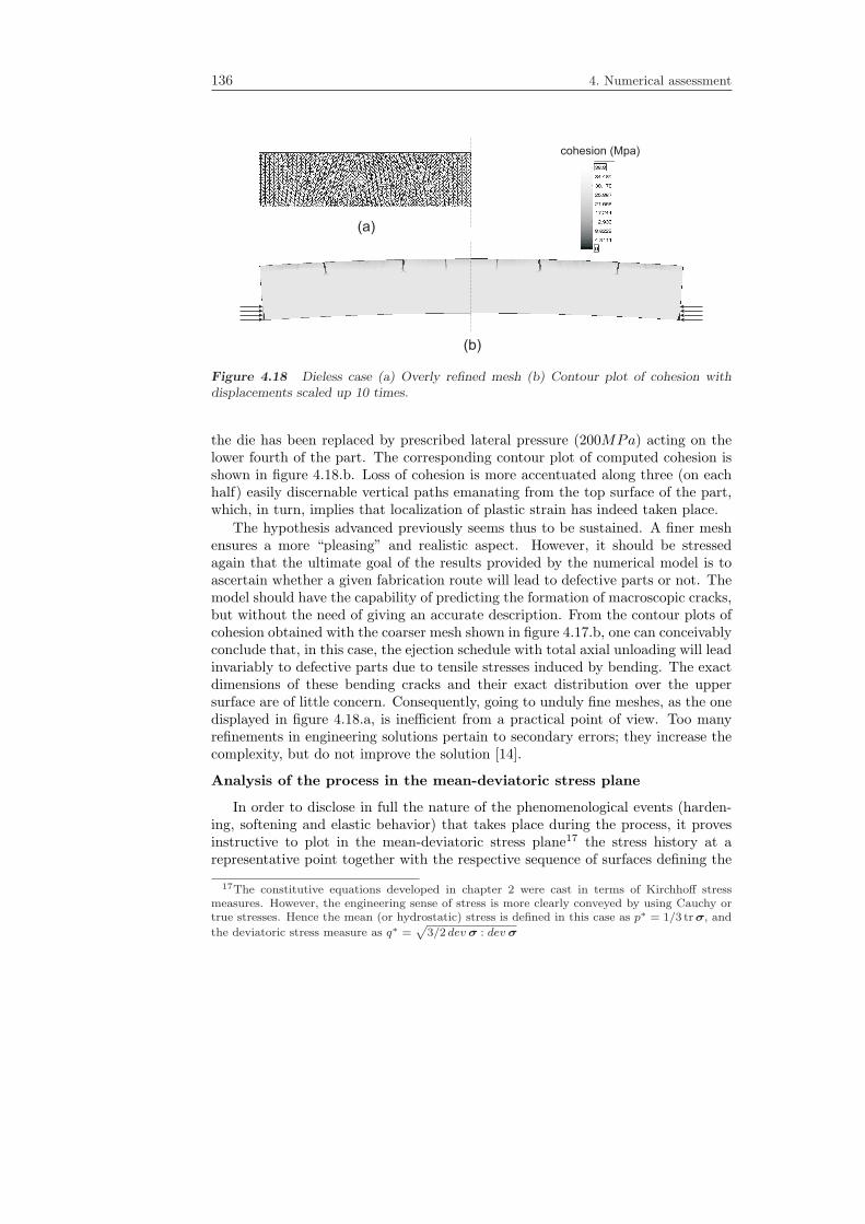
136 4. Numerical assessment
(a)
cohesion (Mpa)
(b)
Figure 4.18 Dieless case (a) Overly refined mesh (b) Contour plot of cohesion withdisplacements scaled up 10 times.
the die has been replaced by prescribed lateral pressure (200MPa) acting on thelower fourth of the part. The corresponding contour plot of computed cohesion isshown in figure 4.18.b. Loss of cohesion is more accentuated along three (on eachhalf) easily discernable vertical paths emanating from the top surface of the part,which, in turn, implies that localization of plastic strain has indeed taken place.
The hypothesis advanced previously seems thus to be sustained. A finer meshensures a more “pleasing” and realistic aspect. However, it should be stressedagain that the ultimate goal of the results provided by the numerical model is toascertain whether a given fabrication route will lead to defective parts or not. Themodel should have the capability of predicting the formation of macroscopic cracks,but without the need of giving an accurate description. From the contour plots ofcohesion obtained with the coarser mesh shown in figure 4.17.b, one can conceivablyconclude that, in this case, the ejection schedule with total axial unloading will leadinvariably to defective parts due to tensile stresses induced by bending. The exactdimensions of these bending cracks and their exact distribution over the uppersurface are of little concern. Consequently, going to unduly fine meshes, as the onedisplayed in figure 4.18.a, is inefficient from a practical point of view. Too manyrefinements in engineering solutions pertain to secondary errors; they increase thecomplexity, but do not improve the solution [14].
Analysis of the process in the mean-deviatoric stress plane
In order to disclose in full the nature of the phenomenological events (harden-ing, softening and elastic behavior) that takes place during the process, it provesinstructive to plot in the mean-deviatoric stress plane17 the stress history at arepresentative point together with the respective sequence of surfaces defining the
17The constitutive equations developed in chapter 2 were cast in terms of Kirchhoff stressmeasures. However, the engineering sense of stress is more clearly conveyed by using Cauchy ortrue stresses. Hence the mean (or hydrostatic) stress is defined in this case as p∗ = 1/3 tr σ, and
the deviatoric stress measure as q∗ =p
3/2 devσ : devσ

4.3 Pressing and ejection of a thin cylindrical part 137
p*, Cauchy mean stress, MPa
q*,
C
au
ch
y d
evia
toric s
tre
ss,
MP
a
E
F
G0 2 4 6 8 10 12 140
5
10
15
20
25
30
35
40
Decrease of cohesion
p*, Cauchy mean stress, MPa
q*,
C
auch
y d
evia
toric s
tre
ss,
MP
a
-700 -600 -500 -400 -300 -200 -100 0
0
50
100
150
200
250
300
350Von Mises yield surface
Elliptical yield surface
Drucker Prager failuresurface
A
E
B
C
D
(a)
(b)
Pressing
Pre
ssur
ere
leas
e
Pre
ssure
rele
ase
( )r z
s = s
z
r
s
<
s
z
r
s>
s
Eje
ction
zs
rs
( 0, )res
z r rs = s =s
Drucker Prager failuresurface
Figure 4.19 Stress trajectory in the mean-deviatoric stress plane of a point located onthe top face of the part. (a) Pressing (path AB), release of axial load (path BCD) andejection (up to the onset of bending, path DE). (b) Enlarged view of the first quadrant.Path EF represents elastic loading due to tensile bending stresses. Path FG indicatesdecrease of cohesion (green strength) due to strain softening.
yield condition.Figure 4.19.a represents the stress evolution at a node located close to the upper
face of the part. During the pressing stage, the stress state traces the path AB.The monotonically increasing character of this loading history ensures that the

138 4. Numerical assessment
powder is always at yielding during this phase. The strength of the material thusraises progressively. This hardening behavior is indicated by the expanding yieldsurfaces (dashed lines). The yield surfaces drawn with a solid line represents theyield condition at the end of the pressing stage. Within the region enclosed bythese yield surfaces, the behavior of the material is presumed to be elastic.
During axial unloading, the stress state follows a piecewise approximated lin-ear path BCD. The yield condition is not affected during this phase, since theentire trajectory lies within the elastic region and, thus, mechanical properties arenot altered. By definition, the deviatoric stress measure q∗ must remain positive.Thereby, the descending tendency of the stress trajectory breaks down at point C,at which the trajectory is “reflected”. The slopes (in absolute value) of the descend-ing and ascending branches are consequently identical. An analytical estimationfor this slope is developed in appendix B.3, Eq.(B.3.10). Point C corresponds to ahydrostatic stress state and it marks18 the transition to stress states in which theradial pressure is dominant (σr > σz). At point D, the axial pressure exerted bythe upper punch is totally released.
p*, Cauchy mean stress, MPa
-700 -600 -500 -400 -300 -200 -100 00
50
100
150
200
250
300
350
q*,
C
au
ch
y d
evia
toric s
tre
ss,
MP
a
r = 7.18 g/cm3
r = 7.00 g/cm3
r = 6.78 g/cm 3Pressing
Axial pressure release
D2
B1
B
C
D
C1
D1
B2
C2
r = 7.18 g/cm
r = 7.00 g/cmr = 6.78 g/cm
Figure 4.20 Stress trajectory in the mean-deviatoric stress plane. Pressing and axialpressure release for three different densities.
The removal of the upper punch is followed by the upward movement of thelower punch for ejecting the part out of the die. As the part moves toward thedie exit, the radial stress at the analyzed material point diminishes gradually. Thiselastic unloading process is represented by the descending path DE in figure 4.19.a.When the analyzed point starts emerging from the die, the magnitude of the stress
18Due to the deliberately low value of the friction coefficient, shear stresses are negligible andradial stresses are approximately constant along the radial direction. Hence radial and hoopstresses are identical, and the deviatoric stress measure can be expressed simply as q∗ = |σz−σr|.Hence, q∗ = 0 implies σz = σr. See appendix B.3 for further details.

4.3 Pressing and ejection of a thin cylindrical part 139
at this node practically vanishes, and the stress state remains thus close to theorigin (point E). Ejection progresses and, when half of the part is out of the die,the eccentricity of the lateral force begins to produce the aforementioned bendingdeformation (see figure 4.17.b). As a consequence, the upper portion of the partis stretched, hence put into tension. This bending deformation causes the stressstate to move within the elastic tensile region (first quadrant of the mean-deviatoricstress plane), which is shown in magnified form in figure 4.19.b, until eventuallyreaching the Drucker-Prager failure line at point F . Yielding on this failure surfaceinduces a decrease of cohesion (softening) of approximately 85%, from 35 MPa to5 MPa, and consequently, the Drucker-Prager failure line shifts toward the origin.This is illustrated graphically by the sequence of parallel dashed lines. During thiscontinued yielding, the stress stress traces the path FG.
Observe that, upon total axial unloading, the stress state lies practically on theVon Mises yield surface (point D in figure 4.19.a). We pointed out in section 2.5.5that this yield surface can be also conceivably viewed as a failure envelope associatedwith compressive and triaxial failure mechanisms. Therefore, the closeness of pointD to this threshold gives clear indication that a final density of 7.18 g/cm3 (98 %of the theoretical density) is unduly high and some type of failure, such as radialcrushing, may be thereby imminent. This fact would have escaped notice by merelyexamining the computed distribution of the Von Mises yield strength cv, since, asmentioned in section 2.5.5, the magnitude of this variable results unaffected whenyielding takes place on the Von Mises yield surface19.
In order to further clarify the influence of the final density on the stress stateupon axial pressure release, two additional analysis with lower compaction densitieshave been run. The results are given in figure 4.20. From this diagram, onecan immediately conclude that moderate target densities imply more favorablecircumstances, since points D1 and D2 are relatively far from the critical Von Misesthreshold20. Incidentally, observe that the slopes of the axial unloading paths arepractically identical for the three cases. This observation is in conformity with theinsensitiveness, analytically inferred in appendix B.3 (see figure B.5), of the valueof the slope to changes in the magnitude of the Young’s modulus.
4.3.1.4 Hold down ejection
The key factor to prevent cracking caused by bending of the part is to maintain acertain level of axial load during ejection [112]. The upper punch must accompanythe lower punch in its upward motion, “sandwiching” the part until it is completelyout of the die cavity and thus avoiding the tendency to bend. The modeling of thehold down pressure is accomplished here by simply controlling the displacement ofthe top surface of the upper punch, which is gradually lifted until reduction of theaxial load to the desired level. Due to the negligible character of friction forces,this procedure ensures the constancy of the upper punch pressure during ejection,
19The unavailability of adequate experimental data in this stress regime compelled us to disre-gard the incorporation of softening for this state variable
20For density ρ = 6.78g/cm3, the Von Mises yield surface “reduces” to a point: the intersectionof the other two yield surfaces (see figure 2.16 in section 2.5.4).

140 4. Numerical assessment
cohesion (Mpa)
Figure 4.21 Ejection with a hold down pressure of 13% of the compaction pressure.Contour plots of computed cohesion at the end of the process.
as it can be checked in the axial pressure versus time graph shown in figure 4.22.a(path be).
Figure 4.21 shows the contour plot of cohesion at the end of the ejection phasefor a case with a hold down pressure of 13% of the compaction pressure. Evidencesof mechanical degradation are detected only along the lateral surface. It is cleartherefore, that, as expected, the hold down ejection method has proven useful ineliminating the de-cohesion pattern on the upper portion of the part.
This procedure admits a compelling interpretation in the mean-deviatoric stressplane. In figure 4.22.b, the stress evolution during axial unloading and ejection atthe same material point analyzed previously (see figure 4.19), is drawn for severalhold down pressures. The ejection branches HJ and BG correspond to total ax-ial unloading and 13 % hold down pressure, respectively. In essence, the effect ofkeeping a certain level of axial load is reflected in the mean-deviatoric stress spaceas a translation of the unloading branch HJ , which shifts towards the compres-sion side to BG, so that the final stress state moves far from the tensile region(first quadrant), thus avoiding the formation of tensile cracks. Needless to say, thelarger the hold down pressure, the further the final stress will be from the tensileregion (points E and F ) and, consequently, the likelihood of tensile-type failurewill decrease. However, large hold down pressures may promote other mechanismof failure, such as crushing, and, furthermore, due to the concomitant increase ofradial pressure, the deterioration of the lateral surface will be invariably aggravated.
4.3.1.5 Die exit geometry: Estimation of a proper taper angle
The graph shown in figure 4.23 represents the trajectory, in the r − z plane, ofthe peripherical upper corner node P. Radial displacements are measured withrespect to the undeformed configuration, whereas changes in vertical position arereferred to the top face of the die. The part gradually expands as it moves toward

4.3 Pressing and ejection of a thin cylindrical part 141
Time (s)
Pre
ssu
re ,
(Mp
a)
-s
0 0.2 0.4 0.6 0.8 1 1.2 1.4 1.60
100
200
300
400
500
600
700 a
a’
b e
e’
b’
c
c’
d
d’
f
g
f’g’
Axial
Radial
Hold down press.13%
Hold down press. 35%
Hold down press. 45%
(a)
p*, Cauchy mean stress, MPa
-700 -600 -500 -400 -300 -200 -100 0
q*,
C
au
ch
y d
evia
toric s
tre
ss,
MP
a
0
50
100
150
200
250
300
350
Elliptical yield surface
Von Mises yield surfaceDrucker Prager failure
surface
A
D
E
C
B
F
G
(b)
Pre
ssure
rele
ase
13%
H.D
.
35%
H.D
.
45%
H.D
.
H
J
0%
H.D
.
Figure 4.22 (a) Average axial and radial pressure during compaction for ejectionschemes with different hold down pressures. (b) Stress trajectories in the mean-deviatoricstress plane corresponding to these ejection schedules.
the die exit. The extent of this radial expansion becomes more pronounced afteremergence from the die (point b). The path bc is approximately straight, a factthat suggests the elastic nature of radial relaxation. The linear approximation tothis path subtends an angle of 0.47 with the vertical axis. Expansion ceases when

142 4. Numerical assessment
the node P is located approximately 3 mm above the top face of the die.
0 0.005 0.01 0.015 0.02 0.025 0.03 0.035 0.04 0.045-6
-5
-4
-3
-2
-1
0
1
2
3
4
a
b
c
Radial expansion (mm)
Dis
tance to
the t
op fa
ce
of th
e d
ie (
mm
)Computed results
Linear approximation (relaxation)
T0.47ºq =
P
Figure 4.23 Axial versus radial displacement of a peripherical upper corner point P.Path bc corresponds to the trajectory traced by P as the emerged portion of the compactexpands elastically.
As mentioned earlier, the loss of computed cohesion observed along the verticalsurface of the cylinder (see figure 4.16.b) can be interpreted as the formation ofsuperficial cracks (lamination) due to the stress concentration derived from theshaft corner at the die exit. To minimize this deleterious effect, the die exit has tobe provided with a slight taper, so as to control radial expansion. The usefulnessof the information presented in figure 4.23 is therefore evident. The taper can bepatterned after the computer displacement profile contained in this figure (pathbc). Accoding to this profile, the tapered die exit would have to be at least 3 mmheight and with a lead-in angle of 0.47 .
4.3.2 Conclusions
The simulation of the pressing and ejection of a cylindrical part seeks to highlightthe utility of the proposed model in reinforcing the physical understanding of howwell-known crack typologies, namely, bending and lateral lamination cracks, aredeveloped. In addition, this simple example typifies perfectly the process of com-paction, since it touches upon all the relevant issues: pressing, axial unloading,ejection, radial spring-back, development of cracks, etc. Therefore, the distinctphenomenological facets of powder behavior can be grasped easily by analyzing thestress state throughout the process. This task is further facilitated by the approx-imated analytical closed-form solutions derived in B. In-depth study of one simple

4.3 Pressing and ejection of a thin cylindrical part 143
case is always of great assistance in anticipating and interpreting results for morecomplex examples.
The de-cohesion patterns observed in the contour plots shown in figure 4.16.ademonstrates the ability of the model to detect evidence of macroscopic defects.The format in which the results are displayed is certainly advantageous from apractical point of view, as it dispenses with the need for either jointly interpretingseveral stress contours, or scrutinizing density distributions to find “suspiciously”intense gradients.
As pointed out at the outset of this chapter, a rigorous quantitative validationof the model, as far as formation of crack is concerned, is somewhat elusive. Theassessment of the calculated results in this example is thus largely qualitative. Forinstance, comparison of the contour plots of computed cohesion shown in 4.17.b and4.21 reveals that maintaining a certain level of axial pressure during ejection assistsin avoiding flexural cracks. This numerical prediction concurs with well-knownexperimental and industrial findings. Therefore, the numerical model proves usefulin qualitatively evaluating the influence, in the formation of cracks, of variationsin the input data (material parameters, tooling kinematics, etc.).
The qualitative nature of the numerical predictions restricts somewhat the spec-trum of practical questions that can be conceivably answered by our approach. Itis important to be aware of such limitations and guard against unrealistically highexpectations. We mentioned that the graph of the trajectory of an upper peripher-ical point during ejection, shown in figure 4.23, suggests somewhat the dimensionsof the taper at the die exit. However, it cannot be expected that the informa-tion contained in such graph provides the exact taper lead-in angle that ensures alamination-free part. To account for the uncertainty associated the calibration ofthe material parameters and the unavoidable modeling errors, one has to performseveral runs with different input data so as to assess the effect of such variations andto obtain a more reliable impresion of the “true” answer. Computer simulationsare there to support engineering judgement, not to supplant it.
The study of convergence with time discretization has shown that, in computingthe pressing stage, the use of variable time steps is essential for avoiding needlesslysmall increments and, therefore, exploiting to the maximum the computationaladvantages offered by the IMPLEX integration scheme. Adequate time step dis-tributions can be obtained by using either adaptive time stepping schemes, of thetype described in Ref. [79], or from elaborated heuristics taking into account theinherent non-linearity of the material. By contrast, in computing the post-pressingoperations, the use of variable time steps only improves marginally the computa-tional efficiency, since in this case the non-linearity of the problem is due largely tothe roughness of the contact response rather than to material behavior.
Although the theoretical aspects of the contact problem have not been a topic ofdiscussion in this work, the relevance of the interaction between the compacted partand the tooling in the formation of post-pressing cracks has rendered necessary abrief assessment of the accuracy of two alternative contact algorithms, namely, thepenalty method and the augmented Lagrangian strategy. The conclusion reachedfrom this evaluation is that the augmented lagrangian strategy is more appropriatefor simulating the post-pressing operations. The reason for the rejection of the less

144 4. Numerical assessment
computational costly penalty method is the oscillatory pattern exhibited by thecomputed boundary stresses, which may affect seriously the quality of the results.The main drawback of the augmented Lagrangian strategy is the dramatic increaseof computational cost - up to 8 times- in comparison with the penalty approach.Work in progress is precisely aimed at reducing the computational cost associatedto the modeling of the contact response [78, 40].
Even with this more accurate contact algorithm, an inappropriate time or spa-tial discretization, or any other modeling error may provoke the appearance of “spu-rious” numerical cracks, mainly at the boundary surfaces. The natural inclinationupon casual inspection of contour plots is to accept as “true” these de-cohesionpatterns, especially when they appear in appealing and pleasing crack-like shapes.The risk of misinterpretation is therefore high. For this reason, it is strongly re-commended to check whether the observed loss of cohesion is physically plausibleor, by contrast, it is caused by numerical inaccuracies. This can be convenientlyaccomplished by tracking, in the mean-deviatoric stress plane, the stress historyat a representative point of the affected area. If no anomalous oscillations are de-tected, then the result, in principle, can be trusted. When the stress state is plottedsequentially together with the corresponding yield surfaces, this procedure has theadded benefit of providing a great deal of insight into the phenomenological behav-ior of the material since, depending on the location of the stress state in relationwith the yield surfaces, one can ascertain at each step whether the powder at theanalyzed point is deforming elastically or elastoplastically with either softening orhardening trends.

Chapter 5
Modeling guidelines forindustrial applications:compaction of a multilevelpart
The aim of this chapter is to evaluate the capabilities of the numerical model de-veloped in previous chapters as a tool for assisting in the design and analysis ofPM uniaxial die compaction processes, including both pressing and ejection stages.For this purpose, a detailed case study of the compaction of an axially symmet-ric multilevel adapter in an advanced CNC press machine is performed, focusingexclusively on the truly engineering aspect, thus leaving aside mathematical andnumerical formalities. Such carefully analyzed case will also serve to provide somemodeling guidelines, sketch frequent difficulties, as the unavailability of some inputdata, and reveal relevant technical details that, although probably trivial for pow-der metallurgy technologists, may escape notice by researchers, especially if theypossess a deficient background knowledge of advanced CNC press machines.
The geometry and dimensions of the part are displayed in figure 5.1. A salientattribute is its relatively low height. The finished lengths of the thinner and thickerlevels of the part are 2.7 mm and 5.32 mm, respectively. This means that a smallerror of, say, 0.2 mm, which is in the order of the value of the maximum finalelastic deflection of the longest punch, in describing the position of one of the tool-ing members may induce an unacceptable discrepancy in the predicted density ofabout 0.4 g/cm3, and it needs no further arguments that the success in predictingnumerically the formation of cracks during the ejection phase relies considerablyon the quality of the density and stress distribution computed in simulating thepressing stage. Furthermore, an accurate prediction of tooling deflection is essen-tial for capturing the formation of cracks in the post-pressing operations. Thesecircumstances explain the prominence given to the accurate characterization of the
145

146 5. Modeling guidelines for industrial applications: compaction of a multilevel part
23.34
24.16
28.14
36.8
39.78
44.759
0.9
2
R1
R0.2
R1
Æ
Æ
Æ
Æ
Æ
Æ
0.15
Z
Z
0.15
5.3
22
±0
.09
2.7
±0
.1
4.2
±0
.07
0.2
x 4
5º
Figure 5.1 Geometry of the part (dimensions in mm). The axisymmetric geometry isrevolved 270 for ease of visualization.
tool set and the external loads acting on it in the first part of this chapter (sections5.1 and 5.2). An aspect that receives careful consideration is the description ofpossible deviations from “nominal” or design values of tooling motions. The effect,in terms of final density distribution, of including such deviations is convenientlyassessed in section 5.3.2.
In dealing with the pressing of complex multilevel parts, it is natural to raisethe question of how to approach the ideal tooling motion that leads to uniformdensity throughtout the compact. This question is also addressed in this chapter(section 5.3.3), but only in an exploratory sense, with a view towards stimulatingthe pursue of this line of enquiry in the future, rather than establishing a procedureof widespread applicability.
It should be anticipated that the part was not finally manufactured according tothe geometry shown in 5.1, which corresponds to the initial customer’s specification.Unsurmountable difficulties were encountered in ejecting the part safely from the

5.1 Modeling of the compacting tool set 147
die, and this circumstance dictated a slight modification -inconsequential to theperformance of the finished component- in the original geometry. This modificationturned out to be effective and the part was successfully manufactured according tothe revised design. The goal in section 5.4 is, by means of numerical simulations ofseveral ejection sequences, to explain the reasons behind the difficulties in ejectingthe original part and understand the connection between such difficulties and thesuggested geometry modification.
5.1 Modeling of the compacting tool set
The forces transmitted to the compacting powder during the pressing operation, aswell as the release of such forces during the ejection stage, should be representedas accurate as possible in order to obtain reliable results. Ideally, the entire pressmachine should be modeled, including punches, core rod, die, press fittings, punchplatens and even the mechanical and hydraulic drives. However, the geometricaland physical characterization of all these press members would require a dauntinglabor and a dramatic increase in computational effort. In this work, thus, we shallconsider only those elements directly involved in forming the part, namely, theupper punch and lower punches, the die and the core rod, the so-called tool set [67],which, incidentally, constitutes the tooling sub-system, according to the systemicconception presented in the introductory chapter.
Punch platens, punch holders and punch adapters are excluded from our modelon the basis of their larger rigidity, in comparison with punches, and therefore thenegligible character of their elastic deflections. An assumption intimately connectedwith this simplification is that the vertical displacement prescribed at punch faces incontact with clamp rings is taken directly as the corresponding platen motion. As itwill emerge later, some deviations may be occasionally detected from this assumedbehavior. In this event, the deviation can be incorporated as a perturbation of theexternally applied load.
In figure 5.2.a, we show the schematic of the multi-platen press machine em-ployed in manufacturing the part. The accompanying drawing, figure 5.2.b, rep-resents the tooling assembly included in the modeling. The tool set comprises anupper punch (UP), four lower punches (LIP, LMP, LOP-I and LOP-II), a die anda core rod. Observe that the lower outer punch labelled as LOP-II is mounted onthe die table. Such an arrangement can be considered as a stepped die or “shelf”die configuration [35].
The dimensions of the core rod, die and punches are shown in figure 5.3. Acrucial issue in modeling the tool set is to account for the actual length and thedifferent diameters sections of punches, so as to predict with the maximum level ofaccuracy elastic deflections. Features such as blend fillets to reduce stress concen-trations at change of section are washed out, as the main concern is the study ofthe powder behavior. Factors related to the tool set that are also ignored in ourmodeling are, among others, the magnitude of the clearances between moving tools,the wear resistance of tools and busting and buckling phenomena. Such range ofdetails is important in its own right and should be studied separately.

148 5. Modeling guidelines for industrial applications: compaction of a multilevel part
(b)(a)
CORE ROD (CR)
UPPER PUNCH
LOWERINNERPUNCH(LIP)
LOWERMIDDLEPUNCH(LMP)
LOWEROUTERPUNCH(LOP-I)
LOWEROUTERPUNCH(LOP-II)DIE
DIE CAVITYDIE TABLE
LIPCLAMP
LIP ADAPTER
Figure 5.2 (a) Cross sectional view of the compacting press. (b) Geometric model ofthe tooling items included in the simulation.
5.2 External actions
The effect of mechanical and hydraulic drives is replaced by prescribed conditionson the portion of punch surface in contact with the clamp rings that fasten me-chanically the punches to their corresponding adapters (see figure 5.2). Theseactions represent mathematically the boundary conditions of the governing differ-ential equations, and can be specified as displacement or traction conditions de-pending on the circumstances and the type of press used for compacting the part.
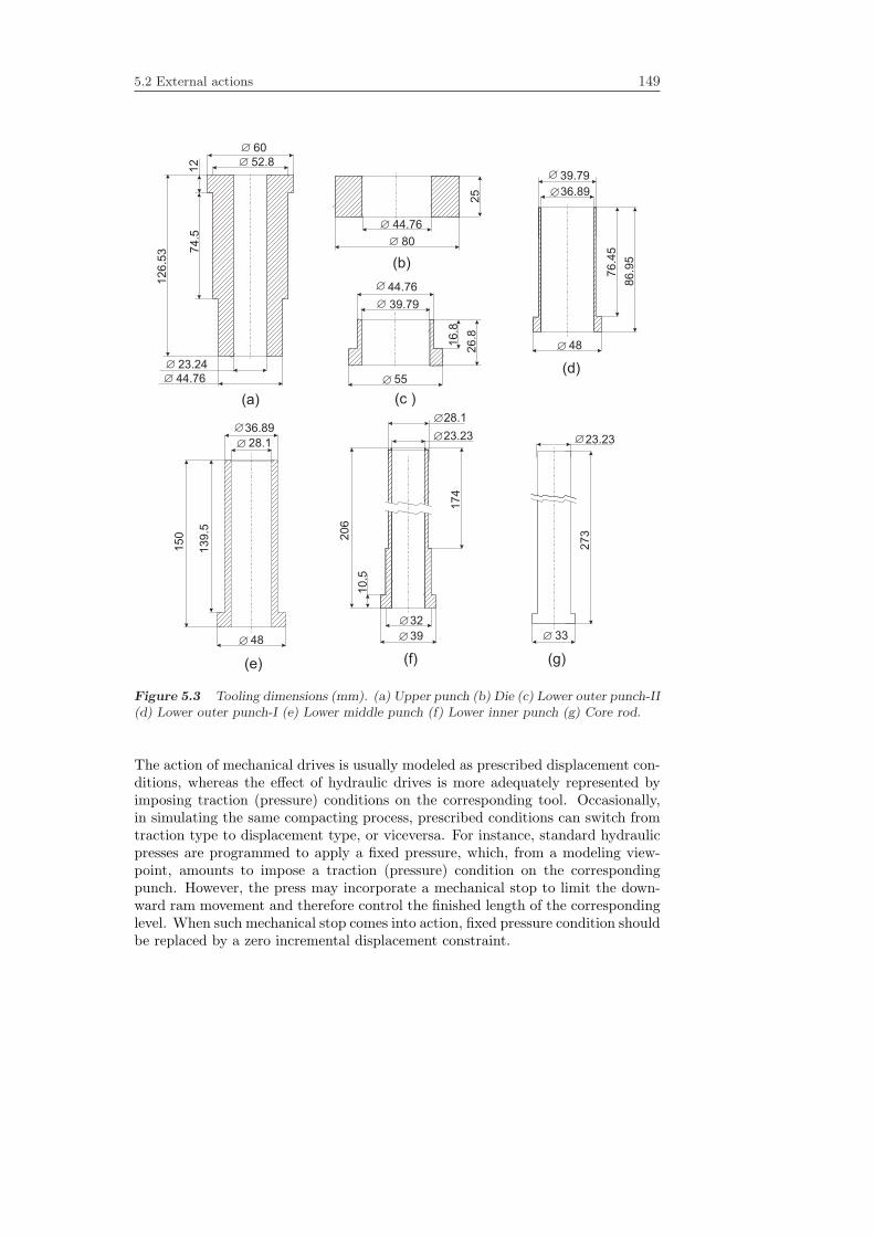
5.2 External actions 149
12
74.5
126.5
360Æ
52.8Æ
23.24Æ
44.76Æ
44.76
44.76
Æ
80
39.79
55
Æ
Æ
25
26.8
Æ
Æ
16.8
76.4
5
86.9
5
48Æ
39.79
36.89Æ
Æ
36.89Æ
48Æ
139.5
150
28.1Æ
39Æ
10.5
206
28.1
23.23Æ
Æ
Æ32
174
273
23.23Æ
Æ 33
(a)
(b)
(c )
(d)
(e) (f) (g)
Figure 5.3 Tooling dimensions (mm). (a) Upper punch (b) Die (c) Lower outer punch-II(d) Lower outer punch-I (e) Lower middle punch (f) Lower inner punch (g) Core rod.
The action of mechanical drives is usually modeled as prescribed displacement con-ditions, whereas the effect of hydraulic drives is more adequately represented byimposing traction (pressure) conditions on the corresponding tool. Occasionally,in simulating the same compacting process, prescribed conditions can switch fromtraction type to displacement type, or viceversa. For instance, standard hydraulicpresses are programmed to apply a fixed pressure, which, from a modeling view-point, amounts to impose a traction (pressure) condition on the correspondingpunch. However, the press may incorporate a mechanical stop to limit the down-ward ram movement and therefore control the finished length of the correspondinglevel. When such mechanical stop comes into action, fixed pressure condition shouldbe replaced by a zero incremental displacement constraint.
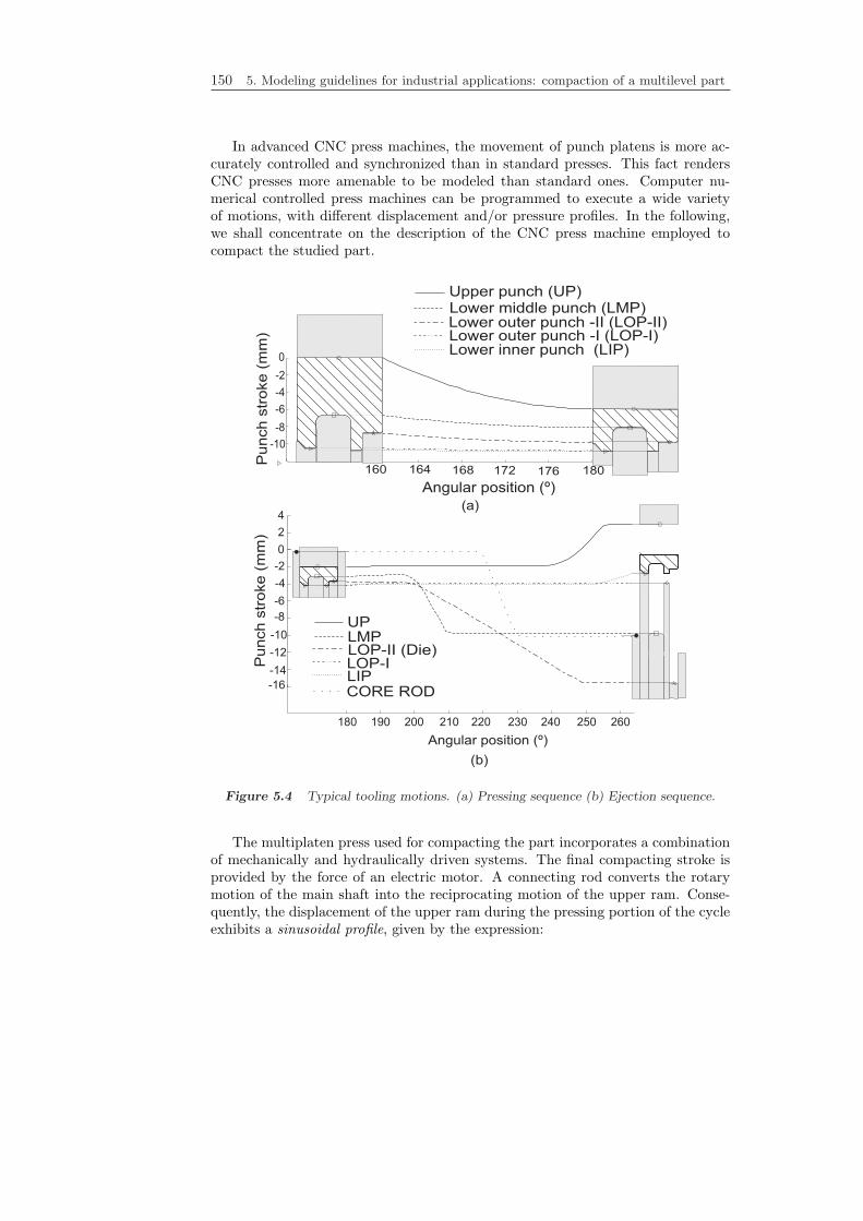
150 5. Modeling guidelines for industrial applications: compaction of a multilevel part
In advanced CNC press machines, the movement of punch platens is more ac-curately controlled and synchronized than in standard presses. This fact rendersCNC presses more amenable to be modeled than standard ones. Computer nu-merical controlled press machines can be programmed to execute a wide varietyof motions, with different displacement and/or pressure profiles. In the following,we shall concentrate on the description of the CNC press machine employed tocompact the studied part.
-10
-8
-6
-4
-2
0
Pu
nch
str
oke
(m
m)
160 164 168 172 176 180
Angular position (º)
Upper punch (UP)Lower middle punch (LMP)Lower outer punch -II (LOP-II)Lower outer punch -I (LOP-I)Lower inner punch (LIP)
180 190 200 210 220 230 240 250 260
0
-2
-4
-8
-10
-12
-14
-6
-16
2
4
Angular position (º)
Pu
nch
str
oke
(m
m)
UPLMPLOP-II (Die)LOP-ILIPCORE ROD
(a)
(b)
Figure 5.4 Typical tooling motions. (a) Pressing sequence (b) Ejection sequence.
The multiplaten press used for compacting the part incorporates a combinationof mechanically and hydraulically driven systems. The final compacting stroke isprovided by the force of an electric motor. A connecting rod converts the rotarymotion of the main shaft into the reciprocating motion of the upper ram. Conse-quently, the displacement of the upper ram during the pressing portion of the cycleexhibits a sinusoidal profile, given by the expression:

5.2 External actions 151
uup =
1−
√1−
(lclrsinϕ0
)2 lr + (1 + cosϕ0)lc, (5.2.1)
where lc and lr stand for the lengths of the crank and the connecting rod, respec-tively, and uup is the pressing stroke, i.e., the distance travelled by the upper ramfrom the onset of pressing (ϕ0) - the position at which the bottom surface of theupper punch enters the die and comes into contact with the powder- to the extremelowest position of the cycle, the so-called bottom dead center, located at ϕ = 180.The rotary motion occurs at constant angular velocity, hence the motion can belegitimately parameterized in terms of the angular position ϕ, as displayed in figure5.4.
During the pressing stage, all elements of the tooling system move downward.The lower punches labelled in figure 5.2.b as LIP, LMP and LOP-I are mounted onseparate platens, whereas the lower outer punch identified as LOP-II is attachedto the die platen. The core rod support is also a movable member, and they all areoperated by hydraulic cylinders placed on the stationary member of the press.
One of the major advantages of using advanced CNC press machines is theflexibility in reproducing any physically realizable motion. The hydraulic drivescontrolling the motion of the lower rams are, in fact, closed-loop motion controlsystems. In our case, the velocity of the lower rams during pressing is kept propor-tional to the velocity of the upper ram, hence their motions also exhibit a sinusoidalprofile, as can be readily appreciated in figure 5.4.a. The angular position and ve-locity of the rotating shaft is monitored at any time during the cycle by a rotaryencoder. This information is sent to a motion controller, which causes the hydraulicdevices to speed up or slow down to correct the velocity of the punch motion so asto keep the proportionality. The following equation expresses such condition:
vp = fp · vup, (5.2.2)
vup is the linear velocity of the upper ram and vp is the downward velocity of anyof the lower rams. Furthermore, the condition of vanishing velocity at the bottomdead center, vup(ϕ = 180) = 0, enables us to write directly
up = fp · uup, (5.2.3)
i.e., given an upper ram pressing stroke uup, the desired stroke for the lower punchescan be adjusted by changing the constant fp. The proportionality parameters fp,henceforth referred to as motion scale factors, must be less than one in order toensure that pressing takes place, and they constitute one of the basic operating pa-rameters of the CNC press machine, that is, parameters that can be easily modifiedby the CNC operator by interacting with the CNC display screen.
In figure 5.4.b, we show the withdrawal type tooling kinematics used in re-moving the analyzed part from the die cavity. It can be readily seen that tooldisplacements are linear functions of the angular position, except in the blend re-gions between paths with different slopes. Observe also that the movement of the

152 5. Modeling guidelines for industrial applications: compaction of a multilevel part
upper punch is not governed by the sinusoidal relation (5.2.1). This is because theupper punch is not connected directly to the rotary main shaft. A hydraulicallycontrolled mechanism, inserted between the upper punch and the upper ram, al-lows independent movements so that, for instance, the upper punch can still applya certain downward load on the compact after reaching the bottom dead center,the so-called counter pressure or top-punch hold-down pressure. In summary, indesigning and modeling the ejection operation, one specifies the prescribed motionof each movable tool as a piecewise linear function. In the case in which the up-per punch is to maintain a certain level of axial pressure, by contrast, one shouldimpose fixed pressure conditions rather than prescribed displacement.
5.2.1 Theoretical and true prescribed conditions
The tooling displacement diagrams described in the preceding discussion and illus-trated in figure 5.4 are the motions that, theoretically, the mechanical and hydraulicdrives impart to the corresponding rams or platens. Quite frequently, in modelingthe compaction process, the displacements prescribed at punch faces in contactwith clamp rings are taken directly as such theoretical platen motions, a tendencyalso observed in the design of PM parts. Furthermore, these displacement curvesare very often simplified to facilitate their handling, eliminating some apparentlyirrelevant details. The resulting data are commonly termed as “theoretical” or“nominal” displacement profiles.
However, departures from this assumed behavior invariably exist. The exact dis-placements of the supported portions of punches, core rod and die seldom coincidewith the theoretical displacement profiles. In analyzing an already manufacturedpart, the “true” motion curves might be at the disposal of the analyst, providedthat the CNC press has displacemet transducers located sufficiently close to thepunch clamps, and in addition, the CNC data acquisition system was set up tostore digitally displacement data so as to enable subsequent handling and analysis.In such circumstances, one should employ the recorded data directly as input datafor the numerical simulation, especially if the scope of the analysis is to simplyreproduce the conditions under which the part was produced.
In other situations, however, as when attacking the design problem or whentesting numerically alternative pressing schedules, true displacement curves arenot available. In such cases, the analyst is faced with the task of having to an-tipate or predict potential deviations from nominal tooling motions. Of invaluablehelp for this purpose is to examine and rationalize the discrepancies between “the-oretical” and “true” motions detected either in compacting parts requiring similarcompaction tonnage - in the case of design analysis - or in producing the same partbut under different pressing and ejection schedules. Not every deviation observedbetween “true” and “theoretical” curves is susceptible to theoretical predictions.We shall distinguish therefore between predictable deviations and unpredictable de-viations.
• Predictable deviations: This group includes those deviations that can be es-timated with a certain degree of accuracy. The analyst should have some

5.2 External actions 153
grasp of the press machine performance in order to ascertain the origin ofsuch discrepancies. An comprehensive listing of all realizable predictable de-viations is not possible, since they depend largely on the nature of the CNCpress machine employed in manufacturing the part. We summarize the mostrelevant predictable deviations encountered in our analysis.
(a) Deviations due to a poor characterization of the tooling subsystem.The fact that only punches, core rod and die are included in the model intro-duces an unavoidable error. Excluded press members, such as punch holders,punch adapters and platens also deflect under high pressures. However, themajor contribution to this modeling error can be attributed to the existenceof adjustable mechanisms inserted between a punch and its correspondingplaten. In the analyzed press machine, for instance, the force exerted by thehydraulic drives on the lower rams is transmitted to the lower punches througha practically rigid assembly of mechanically fastened elements . Hence, littledeviation is expected. By contrast, the hydraulically controlled mechanisminserted between the upper punch and the upper ram, alluded to earlier, con-tributes considerably to the discrepancy between theoretical and true upperpunch motion because of the inevitably looseness (play) of the parts involvedin such mechanism. To calibrate such error in full load operation, one has tofirst measure the deviation in idle conditions, i.e., by compressing an emptydie, and then consider that, approximately, the error increases linearly withincreasing compacting pressure.
(b) Deviations due to overloading of lower rams. In CNC presses in whichthe stroke of lower punches is displacement-controlled during pressing, onecannot ignore the limited capacity of the hydraulic devices that governs theirmotions to sustain any applied force. If the programmed press kinematicsinduces a unduly high density, and consequently a high force, the servosystemcontroller may be pushed out of its regular operating conditions and the lowerram will simply descends maintaining the level of pressure approximatelyconstant, and thus not obeying the scheduled motion. Such deviation canbe included in the simulation by simply shifting the condition of prescribeddisplacement to prescribed traction on the affected lower punch when thecorresponding force threshold is exceed. Later on, the impact of overlookingsuch limited capacity will be assessed in terms of density distribution.
(c) Deviations due to interpolation of punch motions. As can be checkedin figure 5.5, the actual position of the corresponding platens is slightly al-tered in the blended portions of the displacement diagrams. These devia-tions may be of the order of magnitude of the elastic deflection of the longerpunches, hence their effect should be included when studying the ejection pro-cess. Furthermore, tooling displacement diagrams exhibiting sharp cornersare physically unacceptable, since they imply instantaneous change of veloc-ity and therefore infinite accelerations. In practice, velocity is ramped up ordown gradually so as to avoid these unrealistic accelerations (see figure 5.5).These details are normally ignored in designing - and also very frequentlyin modeling - the compaction process, mainly due to obvious simplicity rea-

154 5. Modeling guidelines for industrial applications: compaction of a multilevel part
248 250 252 254 256 258 260
-0.4
-0.2
0
0.2
Angular position (º)
LP
I P
late
n m
otion (
mm
)
True
Theoretical
Figure 5.5 Theoretical and true motion of the lower inner punch platen at the end ofthe ejection stage.
sons. However, from the numerical standpoint, one cannot underestimate thebenefits arising from using the actual smooth displacement profiles insteadof the sharp ones. In general, computability is affected adversely by roughinput data [6]. This is evident in the case of dynamic analysis. More subtle,although equally important, is its implications in the numerical integration ofthe constitutive equation. As pointed in section 3.3, the degree of accuracyof the IMPLEX integration scheme hinges to some extent on the input datasmoothness. All the numerical simulations shown in the sequel employ inter-polated punch trajectories, with peaks rounded using cubic (spline) blends.
• Unpredictable deviations. This group embodies those deviations that displaya distinctly random pattern and, thus, cannot be predicted on the basis of adeterministic analysis. The impact of the individual and combined effect ofsuch deviations can be only evaluated by statistical analysis.
It should be remarked that the borderline between predictable and unpre-dictable deviations depends largely on the beholder and the degree of knowledgeon the press machine. As experience accumulates, initially presumed unpredictablediscrepancies can be converted into predictable ones. Conversely, presumably fore-seeable deviations turning into uncontrolled perturbations may indicate misfunctionof any of the press machine elements or poor maintenace conditions.
5.3 Simulation of the pressing stage
5.3.1 Estimation of the starting conditions
In modeling the pressing stage of an already manufactured part, one should haveat one’s disposal not only an accurate description of the tooling motion, but alsoreliable data concerning the starting conditions of the process. Such starting con-ditions include the fill position of the lower punches, for calculating the fill heightcorresponding to each thickness level, and the powder fill density distribution. In

5.3 Simulation of the pressing stage 155
realistic circumstances, however, the direct determination of such starting con-ditions may be plagued by some difficulties. The CNC data acquisition systemusually monitors only absolute position of punch platens. Knowing with sufficientaccuracy, say ±0.1mm, the position of the bottom face of lower punches wouldrequire thus careful measurements of the length of the assembly of press membersconnecting lower rams and punches. This may be somewhat difficult to achieveif, for instance, the die set has been removed and disassembled for repairing whentackling the computer analysis.
In view of such circumstances, we shall outline in the ensuing discussion theprocedure followed here to confront the unavailability of reliable information con-cerning the aforementioned starting conditions. Incidentally, observe that the un-availability of such data creates an scenario very similar to that encountered in theanalysis of a trial design, in which one has to guess appropriate initial die cav-ity dimensions consistent with the finished lengths of each of the levels within thecompacted part. Thus, the procedure described in the sequel is merely an inverseanalysis, typically used in PM designing. The peculiarity that renders, in our case,this inverse analysis worthy of special consideration arises from the combination oftwo facts: tool motions are non-linear functions of the angular position (time), andpunch elastic deflections have to be included in the calculation of the die cavitydimensions.
Lup
hlmp0
Llmp
Lup
hlmp
LupD-
Llmp LlmpD-
uup
ulmp
180ºjº
Lower middlepunch (LMP)
Upper punch(UP)
Angular position
Figure 5.6 Pressing sequence, indicating motion of the upper punch and the lowermiddle punch. The angle ϕ0 denotes the point in the cycle at which the upper punchenters the die cavity. The pressing stroke ends at ϕ = 180, which corresponds to thebottom dead center.
The fundamental relation between the prescribed displacement on a given punchand the height of the level formed by this punch is illustrated in figure 5.6 for the

156 5. Modeling guidelines for industrial applications: compaction of a multilevel part
particular case of the lower middle punch (LMP). This relation can be expressedanalytically as
h0lpm − hlpm = uup(ϕ0)− ulpm(ϕ0)− (∆Lup + ∆Llpm). (5.3.1)
The meaning1 of each term of the above equation is also clarified in figure 5.6. Thequantity hlpm is the length, measured at the end of the pressing stage (ϕ = 180),of the level formed by the lower middle punch . This length is approximately thelength measured upon ejection from the die, except for a small correction due tospring-back. The depth of fill or fill height corresponding to the thickness levelformed by the LMP is denoted by h0
lpm, and it is defined as the distance from theworking end of the upper punch to the working end of the lower middle punchwhen pressing commences2 (ϕ = ϕ0). The displacements prescribed at the topand bottom surfaces of upper and lower middle punch are symbolized by uup andulpm, respectively. As already discussed, the shape of the displacement profiles are,theoretically, sinusoidal (see Eqs. 5.2.1 and 5.2.3), although they may be eventuallyaffected by some deviations. Finally, the terms ∆Lup and ∆Llpm stand for the totalelastic deflections in the axial direction experienced by the upper punch and thelower middle punch, respectively.
Similar equations to Eq.(5.3.1) can be derived for the other three thicknesslevels:
h0lpi − hlpi = uup(ϕ0)− ulpi(ϕ0)− (∆Lup + ∆Llpi). (5.3.2)
h0lpo′ − hlpo′ = uup(ϕ0)− ulpo′(ϕ0)− (∆Lup + ∆Llpo′). (5.3.3)
h0lpo′′ − hlpo′′ = uup(ϕ0)− ulpo′′(ϕ0)− (∆Lup + ∆Llpo′′). (5.3.4)
Expressions 5.3.1 to 5.3.4 form a system of four equations - one equation foreach lower punch, with ten unknowns: the fill heights corresponding to each level(4 unknowns), the elastic deflections of punches (5 unknowns), and the angularposition at which the upper punch comes into contact with the powder (1 unknown),denoted as ϕ0. The elastic deflections ∆L• can be estimated either on the basis ofavailable data for similar parts, or by means of the uniaxial approximation:
∆L• =σz(ρf )Etool
nr∑
k=1
R21 −R2
i
R2k −R2
i
L•. (5.3.5)
The above equation follows from assuming that an uniaxial stress state prevailsthroughtout the tubular punch. The constant Etool is the Young’s Modulus char-acterizing the tooling material whereas Ri stands for the inner radius of the cor-responding tubular punch and Rk (k = 1, 2, . . .) denotes the outer radii of eachcross section of the punch, sorted by increasing magnitude. The magnitude of thepressure σz(ρf ) acting on the punch face can be estimated from the compressibilitycurve3 as the axial pressure corresponding to the final density ρf of the compact.
1The prefix “lpm” identifies the lower punch that forms the corresponding level of thickness2We further assume that the time at which the lower punches are established in their filling
positions and the time at which the upper punch comes into contact with the powder coincide.3The analytical expression for this curve can be derived by combining material curves s1 and
s2, see Eq.(B.3.11) in appendix B.

5.3 Simulation of the pressing stage 157
Substituting these estimations for the elastic deflection of punches in equations5.3.1 to 5.3.4 leads to a system of four equations with five unknowns, namely the4 fill heights and the initial angular position. The closure for this system, as maybe surmised, is provided by the conservation of mass equation:
ρ0V0(h0lpi, h
0lpm, h
0lpo′ , h
0lpo′′) = ρfVf (hlpi, hlpm, hlpo′ , hlpo′′). (5.3.6)
wherein ρ0 and ρf are the initial and final density, respectively, V0 stands forthe volume occupied by the powder at the onset of pressing and Vf denotes thevolume of the finished part. Note that, in writting Eq.(5.3.6), the hypothesis of uni-form powder fill density4 distribution has been tacitly invoked. This hypothesis isadopted in the absence of further information in this respect. If more accurate dataconcerning this distribution were available, the left-hand side member of Eq.(5.3.6)would have to be replaced by the corresponding integral expression.
To obtain the solution of the resulting system of equations, the values of theunknown quantities h0
• have to expressed as a function of h• and u•(ϕ0). Uponsubstitution of h0
• in Eq.(5.3.6), the system is reduced to a single equation in theunknown ϕ0. Due to its non-linear character, this equation is not amenable toanalytical solution and, consequently, recourse to approximate algorithms, as thebisection method, is to be made. Once the angular position ϕ0 has been obtained,the dimensions of the initial cavity h0
• can be retrieved from equations 5.3.1 to5.3.4.
With these estimated starting conditions at our disposal, we have all the basicingredients to construct the geometric model, impose boundary conditions and,finally, undertake the finite element analysis of the pressing stage. Nevertheless,it is by no means guaranteed that the final lengths computed in this preliminaryFEM analysis will correspond to the desired design values h•. The closeness of thecomputed values to h• relies on the quality of the deflection estimations. A poorestimation of ∆L• will invariably lead to incorrect final dimensions. In our case,the relatively small thickness of the part (2.7 mm in its thinner lever) aggravatesthe situation, since such inaccuracies in estimating ∆L• will translate in innacuratedensity predictions.
A strategy that proves efficient in successively improving the quality of theseestimations is to use the punch deflections computed in the FEM analysis as theestimations for a subsequent reverse analysis. This iterative strategy is schemati-cally described in the flowchart displayed in figure 5.7. Iterations are halted whenthe difference between computed finished lengths and design values h• are withinprescribed tolerances. In our case, such tolerances are taken as the dimensional tol-erances contained in the customer’s specification (see figure 5.1). A more in-depthappreciation of this procedure will be gained through the analysis presented in thefollowing.
4The initial density ρ0 is taken in this cases as the apparent density of the powder.

158 5. Modeling guidelines for industrial applications: compaction of a multilevel part
LpD(ini)
(p=UP, LIP ... )
LpD(ini)
LpD(0)
=
k=1
jº
Obtain(k)
hp
0,(k)
(bisection method)
ANALYSISPRESSINGSTAGE (FEM)
Calculate: hp
(k)
LpD(k)
hp
(k)hp- < TOLp
k >k+1
as a function of LpD(k-1)
CHECK RESULTS(density distribution ...)
Initial estimatefor punchdeflections
YES
NO
Figure 5.7 Flowchart indicating the computational cycle used for estimating the initialdie cavity dimensions.
5.3.2 Assessment of the effect of an innacurate descriptionof tooling motions
In this section, the computed results of final density distributions produced byusing theoretical displacement curves as prescribed conditions on tools, on the onehand, and prescribed conditions closer to true tooling motions, on the other hand,will be examined and compared so as to assess the impact of overlooking some ofthe deviations summarized in section 5.2.1.
The powder employed in making the part is a Distaloy AE iron based powderwith apparent density ρapp = 3.25 g/cm3. Material parameters can be obtainedthus from the empirical adjustment presented in chapter 2. Fill density, whichis assumed uniform throughtout the die cavity, is taken as the apparent density.Friction between the powder mass and the faces of the tools-die walls and corerod is modeled via a friction Coulomb law, with coefficient µ = 0.12. The elasticbehavior of the tooling is characterized by a Young’s Modulus Etool = 210GPaand a Poisson’s ratio νtool = 0.3.
The axial symmetry of the part is exploited and the study is concentrated on acharacteristic radial section so that the FEM analysis can be accomplished in two

5.3 Simulation of the pressing stage 159
Figure 5.8 Initial mesh layout.
dimensions. The initial finite element mesh is shown in figure5 5.8. The average sizeof the elements of the powder body is le = 0.25mm, whereas the size of the elementsat the boundaries of punches and die in contact with the powder is, approximately,0.15mm, although features on the bottom faces of the part, as over the lower outerpunch-II, demands smaller elements (≈ 0.05mm) at these locations. Observe thattooling elements are graded from small-size at the boundaries in contact with thepowder to coarser with increasing distance from these surfaces. A glance at figure5.8 also allows us to appreciate the startling contrast between the volume occupiedby the powder die cavity and the volume occupied by the tooling set.
Results using theoretical punch displacements
The theoretical or nominal displacement profile for the upper punch recipro-cating motion can be obtained from Eq.(5.2.1). The values of the lengths of thecrankshaft and the connecting rod appearing in such equation are lc = 90mm andlr = 580mm, respectively. On the other hand, the theoretical motions of lowerpunches, core rod and die are fully determined by the motion scale factors shownin table 5.1. The motion scale factor of the lower outer punch LOP − II and thedie are identical, as they are mounted in the same platen. On the other hand, itfollows from the motion scale factors of LIP and LOP-I that those punches are heldpractically stationary during the pressing stage.
The information tabulated in Table 5.2 serves to illustrate the previously men-
5The working end of the upper punch is not flush with the top surface of the die when theupper punch comes into contact with the powder, as one may expect (see figure 5.8). Nevertheless,this modification, which has been motivated by simplicity reasons in preprocessing the geometry,has no influence in the computed results.

160 5. Modeling guidelines for industrial applications: compaction of a multilevel part
UP LIP LMP LOP-I LOP-II/DIE CORE RODf 1 0.043 0.234 0.019 0.26 0.233
Table 5.1 Motion scale factors
UP LIP LMP LOP-I LOP-IITOLERANCE in h - 0.09 0.10 0.09 0.07
k = 0 ∆L(Uniaxial est.) 0.307 0.352 0.245 0.130 0.036k = 1 ϕ0 = 160.2 ∆L(k) 0.175 0.298 0.123 0.153 0.0241
h(k) − h - -0.162 -0.080 -0.080 -0.068k = 2 ϕ0 = 160.9 ∆L(k) 0.195 0.197 0.167 0.0928 0.0204
h(k) − h - -0.070 0.055 -0.049 0.003
Table 5.2 Iterative procedure for calculating the initial die cavity dimensions. Theo-retical tooling motion case.
tioned procedure for the calculation of the initial die cavity dimensions. The start-ing values of the elastic deflections ∆L are obtained from the uniaxial estimation(5.3.5). The iterative sequence is halted when the discrepancis between the com-puted finished length h(k) and the design value h (see figure 5.1) is within prescribedtolerances. In the first iteration, the convergence tolerance for the lower inner punchis not met, due to a too high initial estimation of its deflection. An additional com-puter run was hence required to achieve consistent starting conditions.
161.5 163.5 165.5 167.5 169.5 171.5 173.5 175.5 177.5 179.52.5
3.5
4.5
5.5
6.5
7.5
8.5
9.5
10.5
Angular position (º)
Dis
tance (
mm
)
hlmp0
hlip0
hlop-i0
hlop-ii0
hlmp
hlip
hlop-i
hlop-ii
LIPLMPLOP-ILOP-II
hlmp
hlop-i
hlop-ii
hlip
Figure 5.9 Distance between working ends of upper punch and lower punches as afunction of the angular position during the pressing cycle. Theoretical tooling motioncase.
In figure 5.9, we show the evolution of the lengths of each thickness level as afunction of the angular position. As expected, these curves mimic the sinusoidal

5.3 Simulation of the pressing stage 161
pattern of the reciprocating motion of the upper ram. The contour plot of thedensity computed - by the finite element method - at the end of the pressingstage is displayed in figure 5.10. The level formed by the lower middle punchexhibits the highest density, whereas the region with the lowest density is locatedabove the lower inner punch. To enable direct comparison with experimentallymeasure densities, the part is divided into five volumes. The averaged density overthose volumes is shown also in figure 5.10. Experimental and computed results arepresented in table 5.3. It is apparent that numerical results barely resemble theexperimental density measures. Discrepancies between numerical and experimentaldata are especially unacceptable in region labelled as five, just over the lower innerpunch.
Density (g/cm )3
6.886.78
7.186.88
6.58
1234
5
6.806.96
7.047.04
6.99 Experimental
FEM
Figure 5.10 Contour plot of density computed at the end of the pressing stage. Theo-retical tooling motion case.
Zone 1 2 3 4 5 Overallρnum (g/cm3) 6.88 6.78 7.18 6.88 6.58 6.91ρexp (g/cm3) 6.80 6.96 7.04 7.04 6.99 6.94
ρnum − ρexp (g/cm3) 0.08 -0.18 0.14 -0.16 -0.41 -0.03
Table 5.3 Comparison between computed densities using theoretical tooling motion(ρnum) and experimentally measured values(ρexp) .
.
Results using “true” punch displacements
We carry out now the simulation of the pressing stage using prescribed condi-tion on tools closer to the tool motions monitored by the CNC computer duringthe compression. The discrepancies between the theoretically predicted and truemotions of LIP, LOP-I, die and core rod are insignificant and the prescribed dis-placements are therefore the same as in the previous case. By contrast, substantialerrors are detected in the description of the upper punch and lower middle punchmotions. Figure 5.11 shows the theoretical and “true” positions of the top face of

162 5. Modeling guidelines for industrial applications: compaction of a multilevel part
155 160 165 170 175 180-37
-34.5
-32
-29.5
-27
-25
Angular position (º)
Upper
punch p
ositio
n (
mm
)
2 mm»uDTheoretically calculatedposition
True position
Figure 5.11 Position of the upper punch ram. Theoretically calculated value (dashedline) and value monitored and recorded by the CNC data acquisition system (solid line).
the upper punch during the pressing portion of the cycle. The position recordedby the CNC data acquisition system exhibits a gradual deviation from the theo-retically calculated reciprocating motion of the main shaft. At the bottom deadcenter, the amplitude of this deviation can be estimated at approximately 2 mm.This deviation is ascribed to the looseness of the parts comprising the hydraulicallyoperated mechanism, alluded to in section 5.2.1, that controls the force exerted bythe upper punch during ejection, and which is located between the upper punchand the upper ram.
Angular position (º)
160 165 170 175 1800
6
12
18
24
30
36
42
48
54
Forc
e o
n L
MP
(Tons)
LMP maximum allowable load
Force computed using pureprescribed displacement conditions on LMP
Figure 5.12 Force on the lower inner punch computed using pure prescribed displace-ment condition on the lower middle punch. The horizontal dashed line indicates thethreshold below which the hydraulic device controlling the LMP platen operates correctly.
In discussing the classification of what we have termed “predictable deviations”

5.3 Simulation of the pressing stage 163
(see section 5.2.1), we pointed out that the hydraulic drives operating the lowerrams execute the scheduled motion only if the resulting force on each punch is belowa certain threshold. In the case of the lower middle punch, the correspondinghydraulic servosystem operates under regular conditions below 25 Tons. Figure5.12 shows the FEM computed evolution of the force exerted by the compactingpowder on the lower middle punch using theoretical tooling kinematics, in whichthe stroke of the lower punches is assumed to be displacement-controlled duringthe entire pressing stage. The information displayed in figure 5.12, however, makesapparent the inadequacy of such assumption. The computed force at the end ofthe end of pressing operation exceeds the maximum allowable force by a factor ofalmost two. This unduly high force on the LMP is intimately connected with theoverdensification observed in the region over the lower middle punch (see figure5.10). According to the suggestion given in section 5.10, the prescribed conditionon the lower middle punch must be modified to accommodate this limited capacityof the hydraulic device. For forces below 25 Tons, displacements given by theexpression ulmp = flmp · uup will be imposed on the bottom surface of the punch.When the force rises slightly above 25 Tons, the displacement condition will bereplaced by a pressure-type condition so as to ensure that the lower middle punchmoves downward maintaining the force in 25 Tons.
UP LIP LMP LOP-I LOP-IITOLERANCE in h - 0.09 0.10 0.09 0.07
k = 0 ∆L(Previous simul.) 0.175 0.298 0.123 0.153 0.0241k = 1 ϕ0 = 156.7 ∆L(k) 0.182 0.325 0.136 0.196 0.016
h(k) − h - -0.0043 -0.057 0.0125 -0.034
Table 5.4 Iterative procedure for calculating the initial die cavity dimensions. “True”tooling motion case.
LIP LMP LOP-I LOP-IIh0• comp. using nominal displacement 10.22 6.70 10.52 8.63h0• comp. using true displacement 10.87 6.47 11.23 8.20
Difference (%) 5.97 -3.54 6.37 -5.35
Table 5.5 Fill heights (mm) corresponding to each thickness level. Theoretical and“true” tooling motion cases.
The simulation of the pressing stage is carried out again with these new bound-ary conditions on both upper punch and lower middle punch, First, we determinethe starting conditions by means of the strategy illustrated in the flowchart con-tained in figure 5.7. The information concerning such procedure is set forth intable 5.4. In the first iteration, the differences between calculated lengths of eachthickness levels and the design values are between the prescribed tolerances, hence,in this case, guesswork is limited to a single computer run6. In table 5.5, we sum-
6The initial estimation of punch deflections employed in this case has been obtained from the

164 5. Modeling guidelines for industrial applications: compaction of a multilevel part
hlmp0
hlip0
hlop-i0
hlop-ii0
hlmp
hlop-ii
LIPLMPLOP-ILOP-II
155 157.5 160 162.5 165 167.5 170 172.5 175 177.5 1802
3.5
5
6.5
8
9.5
11
Angular position (º)
Dis
tance (
mm
)
hlip hlop-i»
hlmp
hlop-i
hlop-ii
hlip
Figure 5.13 Distance between working ends of upper punch and the lower punches asa function of the angular position during the pressing cycle.“True” tooling motion case.
marize the fill heights corresponding to each thickness level calculated on the basisof theoretical and “true” prescribed conditions. According to such data, includingthe aforementioned deviations in the UP and LMP motions implies changes onthe die cavity dimensions of, on the average, 5%. The variation during pressingof the lengths of the levels formed by each lower punch is depicted in figure 5.13.The effect of the alluded to earlier deficient transmission of motion between theconnecting rod and the upper punch is apparent, as the curves do not display thecharacteristic sinusoidal shape observed in the prescribed displacement case.
6.786.92
7.106.94
6.91
1234
5
6.806.96
7.047.04
6.99Experimental
FEM
Figure 5.14 Contour plot of density computed at the end of the pressing stage. “True”tooling motion case.
first iteration in computing the starting conditions of the theoretical motion case (see table 5.2).

5.3 Simulation of the pressing stage 165
Density contours at the end of compression are shown in 5.14, accompaniedby computed averaged density within the analyzed subdomains. These averagedvalues are compared with experimental measures in both figure 5.14 and table5.6. Clearly, numerically predicted densities obtained with the model using “true”tooling motions correspond more closely with empirically measured densities thanin the theoretical tooling motion case (see figure 5.10). Furthermore, the agreementcan be deemed satisfactory, as differences are within 0.1 g/cm3. This comparisonyields convincing proof of the importance of having an accurate description ofthe pressing motion at one’s disposal if one wishes to bring computed results intoquantitative agreement with experimental data, especially if the analyzed part isrelatively thin.
Zone 1 2 3 4 5 Overallρnum (g/cm3) 6.78 6.92 7.10 6.94 6.91 6.93ρexp (g/cm3) 6.80 6.96 7.04 7.04 6.99 6.94
ρnum − ρexp (g/cm3) -0.02 -0.04 0.06 -0.10 -0.08 -0.01
Table 5.6 Comparison between computed densities using “true” tooling motion (ρnum)and experimentally measured values(ρexp) .
5.3.3 Optimization of the pressing sequence
Inspection of the contour plot contained in figure 5.14 reveals that the densityfield obtained with the tooling motion analyzed in the previous section exhibits aconsiderable degree of non-uniformity. For instance, the averaged density in thepowder column formed by the lower outer punch LOP-II is 0.24 g/cm3 below theaveraged density in the column formed by the lower middle punch. In view ofthis considerable lack of uniformity, it is natural to inquire whether other toolingmotions might have led to more uniform density fields, and how these sequencesof motion can be obtained. This raises the issue of optimization of the pressingsequence, i.e., how to approach the “ideal” tooling motion that leads to an uniformdensity field throughout the compact.
In essence, the strategy followed here to obtain the optimum pressing sequenceis the determination of the tooling motion that ensures a near constant compressionratio7 in each thickness level of the part. This method is, certainly, but the commonmanner in which the dimensions of the fill cavity are calculated in the design stage[100]. However, rather than address the question in this conventional manner8,we couch our discussion in the broader context of optimization problems, so as to
7The compression ratio is defined as the ratio of the height of the loose powder to that of thegreen compact (for each thickness level).
8An added difficulty here is that, on the one hand, tool motions are non-linear functions of theangular position - due to the reciprocating nature of the upper punch motion and the inclusion ofthe previously outlined predictable deviations -, and in the other hand, punch deflections have tobe taken into consideration. It can be shown that, under such conditions, the system of nonlinearequations that arises from imposing the condition of constant compression ratio may have nosolution.

166 5. Modeling guidelines for industrial applications: compaction of a multilevel part
regard the problem from the most general standpoint and, eventually, encouragefurther advances in this line of development.
Objective function
A crucial step in the formulation of any optimization problem is the definitionof the function that has to be minimized, the so-called objective function. In ourcase, this objective function has to measure the degree of non-uniformity of densitydistribution. If we divide the part into n nonoverlapping volumes, an indication ofthe degree of deviation from a state of uniform density is provided by the euclideannorm of the differences between the average density ρi calculated in each volumeand the overall density ρf :
edens =
√√√√n∑
i=1
(ρi − ρf )2. (5.3.7)
The manner in which the part is divided into volumes has a significant influenceon the nature of the solution. Different divisions may lead to distinctly differentoptimal pressing routes. Besides, the complexity in obtaining the solution increaseswith increasing number of subdivisions. A limiting case is to choose the partitionprovided by the own finite element mesh. However, the density in the volumeassociated to a typical finite element is too small to be measured in practice. Witha view towards eventual experimental validation, thus, it proves more convenientto select easily measurable volumes.
As mentioned above, the aim is to devise a tooling kinematics that approachesa constant compression ratio in each thickness level of the compact. This consid-eration leads naturally to the part division sketched in figure 5.15. The compact isdivided by cylindrical surfaces parallel to the pressing direction, resulting in four“column” subdomains, one for each lower punch. The objective function (5.3.7) for
hlmp0
hlip0
hlop-i0hlop-ii
0
hlmp
hlop-ihlop-iihlip
Vlip0
V0lmp
V0lop-iiV
0lop-i
Vlip Vlmp
Vlop-i Vlop-ii
(a) (b)
Figure 5.15 Division of the part in columns. (a) Initial columns (b) Final columns.
this case reads:
edens =√
(ρlip − ρf )2 + (ρlmp − ρf )2 + (ρlop′ − ρf )2 + (ρlop′′ − ρf )2. (5.3.8)

5.3 Simulation of the pressing stage 167
Note that the optimization problem associated to this objective function onlyquantifies density gradients between the columns formed by each lower punch. Vari-ation of density along the pressing direction owing to wall friction is, consequently,completely ignored. For parts of relatively low height, as the one analyzed here, inwhich friction effects do not play a relevant role in determining density distribution,this division in columns proves adequate. On the contrary, for parts of considerableheight, in which density changes promoted by wall friction become dominant, thispartition may fail in providing useful information and the part should be subjectedto additional horizontal subdivision.
In evaluating the objective function (5.3.8), the overall density ρf can be cal-culated from simple mass conservation considerations. The determination of theaverage density in each column requires more elaborate computations: first onehas to obtain the fill heights consistent with the given tooling motion the finishedlengths of the part - following the procedure outlined in section 5.3.1 - and then tolaunch the finite element analysis so as to finally determine these average densities.
Variables or parameters of the problem
The following step in the formulation of our optimization problem is to definethe so-called design variables or parameters. All controllable factors, related withthe press kinematics, whose variation affects to some extent the final density distri-bution can be included in this group. The logical candidates for being considered asthe design variables of our optimization problem are the set of motion scale factors,as they entirely characterize the tooling motion. In order to reduce the numberof variables, one of the lower punches that forms the lowest face of the part, theLOP-I, is assumed to remain stationary, that is, flop′ = 0. The motion scale factorassociated to the core rod is also excluded from the variables or parameters of theproblem, as it induces only density gradients in the pressing direction, which arepractically inconsequential to the value of the objective function. We are left thuswith a total of three variables, namely, the motion scale factors of the LIP, LMPand LOP-II, or expressed symbolically f = [flip, flmp, flop′ ]. The problem can bemathematically posed as the determination of the motion scale factors f that min-imizes the objective function (5.3.8). This problem falls under the general rubric ofnonlinear constrained optimization problems. The constrained character refers tothe fact that the value of the motion scale factors must lie in the interval [0, 1]. Azero value amounts to keep fixed the corresponding lower punch during the entirepressing stage, whereas a motion scale factor equal to one means that the lowerpunch moves downward at the same velocity as the upper punch and, thus, noeffective pressing takes place. The problem is nonlinear because of the nonlinearcharacter of the relation between the objective function and the variables.
Solution of the optimization problem. Simplified “column” model.
This nonlinear constrained optimization problem can be attacked, as done for in-stance in Ref. [57], by recourse to the standard optimization techniques describedin the related literature [71, 85, 19]. However, the discussion of the formalisminvolved in such techniques, as well as their adaptation to the problem of optimiza-tion of the pressing sequence, are huge and complex topics in their own right, and

168 5. Modeling guidelines for industrial applications: compaction of a multilevel part
falls thereby beyond the scope of this work. Here, we limit ourselves to providea reliable approximation to this solution. This approximation may be eventuallyused as the starting point9 for solving the problem by the aforementioned elaborateoptimization algorithms.
To determine this approximation of the minimizer of the original functionalobjective (5.3.8), we introduce an alternative model for replicating the powderbehavior. The essence of this model is intimately connected with the division incolumn subdomains shown previously in figure 5.15. Each powder column is treatedas a separate component, in the spirit of the “column model” described in reference[103]. This means that transfer of mass between columns is neglected. Densificationon each domain can be studied thus by simply applying the conservation of massequation:
ρcollp = ρ0V 0lp(h
0lp)
Vlp(hlp), (5.3.9)
where ρcollp denotes the column average density at the end of compression, ρ0 isthe fill density (assumed uniform), and V 0
lp(h0lp) and Vlp(hlp) the initial and final
volumes, respectively, of the column corresponding to the lower punch labelled as“lp”. Now we define, in analogy with (5.3.8), the following objective function:
ecoldens =√
(ρcollip − ρf )2 + (ρcollmp − ρf )2 + (ρcollop′ − ρf )2 + (ρcollop′′ − ρf )2. (5.3.10)
This “column model” is indeed a very crude approximation to reality, and, in gen-eral, the values of density predicted by the elementary estimation (5.3.9) woulddiffer substantially from the values computed by the more sophisticated and real-istic finite element model. In situations in which overdensification in one columntakes place at the expense of deficient consolidation in the adjoining regions, thediscrepancies would be particularly drastic. In circumstances, on the contrary, inwhich transfer of mass between columns is not pronounced, the two estimationswould be more in agreement. Accordingly, the minimum difference between bothpredictions would be detected in the case in which redistribution of mass betweencolumns is, on the average, minimum. It follows from this physically plausiblereasoning that the minimizer of the objective function (5.3.10) associated to theelementary column model can be regarded as an approximation of the minimizerof the objective function associated to the finite element model. The quality ofthis approximation must be eventually assessed by undertaking a finite elementanalysis.
The advantage of this strategy relies on the fact that the solution of the opti-mization problem linked to the column model is comparatively easy to obtain. Thenumber of variables is only three, and the evaluation of the objective function is,computationally speaking, inexpensive. Consequently, evaluation of the function
9Standard optimization techniques are based in iterative schemes. The number of iterations toachieve convergence relies mainly on the closeness of the starting point to the solution. In view ofthe high computational cost associated to each evaluation of the objective function, the processmay become prohibitively expensive if the choice of starting point is not adequate.

5.3 Simulation of the pressing stage 169
0.6000.5250.4500.3750.3000.2250.1500.0750.000
L0P-II velocity factor (f )
0 0.1 0.2 0.3 0.4 0.5 0.60
1
2
3
4
0 0.1 0.2 0.3 0.4 0.5 0.60
1
2
3
4
0 0.1 0.2 0.3 0.4 0.5 0.60
1
2
3
4
0 0.1 0.2 0.3 0.4 0.5 0.60
1
2
3
4
0 0.1 0.2 0.3 0.4 0.5 0.60
1
2
3
4
e(g
/cm
)dens
3e
(g/c
m )
dens
3e
(g/c
m )
dens
3
e(g
/cm
)dens
3e
(g/c
m )
dens
3
lop-ii
LMP velocity factor (f )lmp
LMP velocity factor (f )lmp LMP velocity factor (f )lmp
LMP velocity factor (f )lmp LMP velocity factor (f )lmp
f = 0lip
f = 0.15lip
f = 0.45lipf = 0.60lip
f = 0.30lip
Optimum solution
Figure 5.16 Objective function edens as a function of motion scale factors. The lowerouter punch (I) is held stationary in all cases, i.e., flop′ = 0, whereas the motion scalefactors of the other lower punchers are varied from 0 to 0.6.
at a sufficient number of points so as cover the entire range of these variables (thefeasible region [71]) is computationally affordable. The minimum can be directlyobtained as the lowest value of the vector resulting from such evaluations. We

170 5. Modeling guidelines for industrial applications: compaction of a multilevel part
should remark, however, that this straightforward, although certainly not very el-egant, way of finding the solution may be not feasible in other cases, because ofeither the unaffordable computational cost associated with the evaluation of theobjective function or the large number of variables. In those cases, recourse tostandard optimization algorithms should be made.
Further insight into the nature of the solution is gained if these points arerepresented graphically. Figure 5.16 shows five diagrams. Each of these diagramsis a parametric plot, with the LOP-II motion scale factor flop′′ as parameter, ofthe objective function ecoldens versus the LMP motion scale factor flmp, holding fixedflip.
It is readily apparent from these graphs that holding stationary the lower innerpunch (flip = 0) represents the most favorable situation. This concurs with one’sintuitive expectation, as the finished length of the levels formed by the LIP and theLOP-I are identical, hlip = hlop′ . The global minimum is to be sought then in thediagram displayed on the top left corner of figure 5.16. Visual inspection of thisplot indicates that the global minimum is approximately located at flmp = 0.415and flop′′ = 0.225.
UP LIP LMP LOP-I LOP-II/DIEf 1 0.000 0.225 0.000 0.415
Table 5.7 Set of motion scale factors that minimizes the objective function associatedto the elementary column model.
FEM Validation
The combination of motion scale factors10 that minimizes the objective functionassociated to the elementary column model is summarized again for convenience intable 5.7. According to the physical arguments put forward previously, these motionscale factors should lead to a “near” uniform density distribution. To confirm thishypothesis, one must perform a finite element analysis, since the column model istoo simplistic as to accept its results at face value. Thus, only a FEM analysiscan provide the assurance that the presumably near-optimum motion scale factors,listed in table 5.7, define indeed tooling displacements that lead to more uniformdensity distribution.
As usual, to carry out the finite element analysis, we obtain first the fill cavitydimensions consistent with such tooling motion. The iterative procedure is illus-trated in table 5.8. In figure 5.17, the computed evolution of the length of the levelsformed by each lower punch is displayed. Observe that the curves exhibit a verysubtle inflexion point around ϕ = 170, a fact that reflects that the deviation dueto plays in the hydraulic mechanism controlling the position of the upper punchhas been included in constructing the punch displacement profiles.
The average densities in each column subdomain at the end of compressionobtained by the elementary column estimation and by finite element calculations
10The motion scale factor associated to this tool has been set to the one corresponding to theDIE/LOP-II.

5.3 Simulation of the pressing stage 171
UP LIP LMP LOP-I LOP-IITOLERANCE in h - 0.09 0.10 0.09 0.07
k = 0 ∆L(Previous simul.) 0.257 0.249 0.219 0.107 0.0288k = 1 ϕ0 = 157.5 ∆L(k) 0.209 0.324 0.134 0.183 0.0232
h(k) − h - -0.012 -0.152 -0.039 -0.075k = 2 ϕ0 = 157.7 ∆L(k) 0.187 0.312 0.115 0.181 0.0211
h(k) − h - -0.074 -0.062 -0.090 -0.046
Table 5.8 Iterative procedure for calculating the initial die cavity dimensions. Opti-mized tooling motion case.
157.5 160 162.5 165 167.5 170 172.5 175 177.5 1802
4
6
8
10
Angular position (º)
LIPLMPLOP-ILOP-II
hlip hlop-i»
hlop-ii
hlmp
hlop-i0
hlip0
hlop-ii0
hlmp0
Dis
tance (
mm
)
Figure 5.17 Distance between working end of upper punch and lower punches as afunction of the angular position during the pressing stage. Optimized tooling motioncase.
COLUMN LIP LMP LOP-I LOP-II OverallColumn model 6.98 7.02 6.91 6.90 6.96FEM model 6.95 7.04 6.98 6.97 6.98
ρcol − ρfem (g/cm3) 0.03 -0.02 -0.06 -0.08 -0.02
Table 5.9 Averaged densities ((g/cm3)) obtained by the elementary column estimationsand by the finite element calculations.
.
are compared in table 5.9. Discrepancies between both set of values are within 0.08g/cm3. Such satisfactory agreement substantiates the hypothesis of the closenessbetween the minimizers of the original FEM optimization problem and the oneassociated to the column model. Certainly, further improvements in uniformityof the density distribution might be achieved. The density over the lower middlepunch, for instance, (see figure 5.18), is still 0.09 g/cm3 higher than the averagedensity above the lower middle punch. As already pointed out, the determination ofmotion scale factors leading to further improvements would require a local search,

172 5. Modeling guidelines for industrial applications: compaction of a multilevel part
by standard optimization techniques, in the vicinity of the values tabulated in table5.9.
Density (g/cm )
LMP
LIP LOP-I
LOP-II
6.95
7.04
6.986.97
3
Figure 5.18 Contour plot of computed density at the end of compression. Optimizedtooling motion case.
So far, the discussion has been limited to the improvement in uniformity ofthe final density field. One would expect that motion scale factors leading touniform density distribution will also contribute to uniform density fields at anyother point during the pressing operation. In figure 5.19, the variation, with angularposition, of averaged densities in each subdomain is shown for the optimized toolingmotion case and for the tooling motion characterized in the previous section (with“true” displacement profiles). Comparison of these diagrams clearly confirms thisexpectation. The five paths in each case emanates from the same point, whichcorresponds to the fill density (ρ0 = 3.25), and deviates gradually from one anotheras pressing progresses. However these deviations are considerably more pronouncedin the non-optimized case (figure 5.19.a). Especially intense is the magnitude ofthe drift exhibited by the averaged density in the region above the lower middlepunch (zone 3).
A quite relevant result is the magnitude of the forces induced on the punchesduring compression. The FEM computed evolution of these forces is depicted infigure 5.20. Observe that the punch on the lower middle punch remains below25 Tons, which means that the hydraulic drive controlling this punch remains,according to the finite element calculations, within the controlled-displacementregime.
For a rigorous assessment of the proposed methodology, the numerically pre-dicted improvement in density should be experimentally corroborated. Unfortu-nately, owing to unavailability of the press machine, it was not possible to manu-facture the part according to the pressing route determined by the proposed pro-cedure. This experimental validation, as well as the extension of the methodologyto other part geometries in which friction effects are to be accounted for, are leftto future work.

5.4 Ejection 173
Angular position (º)
density (
g/c
m )3
Zone 1
Zone 1
Zone 2
Zone 2
Zone 3
Zone 3
Zone 4
Zone 4
Zone 5
Zone 5
1
1
2
2
3
3
4
4
5
5
156 158 160 162 164 166 168 170 172 174 176 178 1803
3.5
4
4.5
5
5.5
6
6.5
7
Angular position (º)
density (
g/c
m )3
156 158 160 162 164 166 168 170 172 174 176 178 1803
3.5
4
4.5
5
5.5
6
6.5
7(a)
(b)
Figure 5.19 Evolution of averaged density in each volume. (a) Non-optimized toolingmotion (b) Optimized tooling motion.
5.4 Ejection
Attention is confined now to the simulation of the ejection stage. This stage coversapproximately the portion of compaction cycle ranging from 180 to 265, and canbe further subdivided into three distinctly different phases. This division is illus-trated schematically in figure 5.21. The first phase corresponds to partial pressurerelease. The upper punch moves slightly upward so as to reduce radial forces andfacilitate the subsequent withdrawal of the die. This phase covers only a smallportion of the entire ejection operation, from11 180 to 190.
In the second phase, from 190 to approximately 240, the die moves downward
11Considering that the production rate is approximately 660 pieces per hour, the time requiredto carry out a complete cycle can be estimated by tcycle = 3600/660 = 5.45 seconds, and hencethe pressure release stage lasts only about tprel = 5.45 10/360 = 0.15 seconds.

174 5. Modeling guidelines for industrial applications: compaction of a multilevel part
155 160 165 170 175 1800
10
20
30
40
50
60
Forc
e o
n p
unces (T
ons)
Angular position (º)
Upper punch (UP)Lower inner punch (LIP))Lower middle punch (LMP)Lower outer punch -I (LOP-I)Lower outer punch -II(LOP-II)
UP
LIP
LMP
LOP-I
LOP-II
Figure 5.20 Evolution of computed force on punches.
.
180 190 200 210 220 230 240 250 260
0
-2
-4
-8
-10
-12
-14
-6
-16
2
4
Angular position (º)
Pressurerelease
(b)
Die withdrawalUP and LIPupward motion
UPLMPLOP-II (Die)LOP-ILIPCORE ROD
Pu
nch
str
oke
(m
m)
Figure 5.21 Typical tooling motion profile for the ejection stage.
(withdrawal tooling system) while the two lower punches (LIP and LOP-I) formingthe lowest faces remain stationary so as to support the part. In order to releasesome radial pressure, the withdrawal movement of the die may be accompaniedby the downward motion of the core rod and/or the lower middle punch. In thethird stage, ranging from 240 to 265, the upper punch moves up away from thecompact and, simultaneously, the lower inner punch lifts the part slightly so thatit can be removed by the gripper from the compaction zone.
The finite element results will be also presented according to this division of
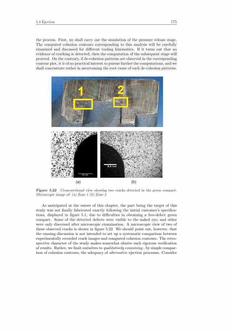
5.4 Ejection 175
the process. First, we shall carry out the simulation of the pressure release stage.The computed cohesion contours corresponding to this analysis will be carefullyexamined and discussed for different tooling kinematics. If it turns out that noevidence of cracking is detected, then the computation of the subsequent stage willproceed. On the contrary, if de-cohesion patterns are observed in the correspondingcontour plot, it is of no practical interest to pursue further the computations, and weshall concentrate rather in ascertaining the root cause of such de-cohesion patterns.
(a) (b)
1 2
Figure 5.22 Cross-sectional view showing two cracks detected in the green compact.Microscopic image of: (a) Zone 1 (b) Zone 2
As anticipated at the outset of this chapter, the part being the target of thisstudy was not finally fabricated exactly following the initial customer’s specifica-tions, displayed in figure 5.1, due to difficulties in obtaining a free-defect greencompact. Some of the detected defects were visible to the naked eye, and otherwere only discerned after microscopic examination. A microscopic view of two ofthese observed cracks is shown in figure 5.22. We should point out, however, thatthe ensuing discussion is not intended to set up a systematic comparison betweenexperimentally recorded crack images and computed cohesion contours. The retro-spective character of the study makes somewhat elusive such rigorous verificationof results. Rather, we limit ourselves to qualitatively examining , by simple compar-ison of cohesion contours, the adequacy of alternative ejection processes. Consider

176 5. Modeling guidelines for industrial applications: compaction of a multilevel part
two alternative routes A and B for ejecting the part from the die cavity. If, forinstance, the cohesion computed using the ejection route A remains unaltered dur-ing the process, whereas the predicted cohesion contours using ejection schedule Bshows clear signs of cracking, we can legitimately say that ejection schedule A is,comparatively, more appropriate than ejection route B. However, we should refrainfrom categorically concluding that ejection schedule A leads to a free defect part,as this would require confirmation from experience.
5.4.0.1 Pressure release
The finite element analysis of the pressure release stage is restarted12 from thesolution (using “true” punch displacement curves, see section 5.3.2) obtained atthe end of the computation of the pressing stage. In the sequel, two differentsequences of tooling motion are examined.
UP
COREROD
DIE
LOP-II
LOP-I
LMP
LIP
Crack ACrack B
gap
Cohesion (Mpa)
Figure 5.23 Contour plot of cohesion at the end of pressure release stage. Total axialunloading case.
.
First, we consider a scenario in which the upper punch moves up away fromthe compact and the lower platens remain fixed. Every PM practitioner knowsthat this practice represents conditions likely to generate a defective part and,thus, is by no means adequate, especially when dealing with relatively thin parts.Nevertheless, we shall momentarily overlook such practical recommendation and
12As alluded to in section 4.1, a restart facility in the simulation code provides the flexibility inautomatically initiating the analysis from any point in the computational cycle. In restarting theanalysis, some parameters controlling the solution algorithm can be changed. For instance, for theejection stage, kinematic description is restricted to the small strain regime and the remeshingutility is disabled.
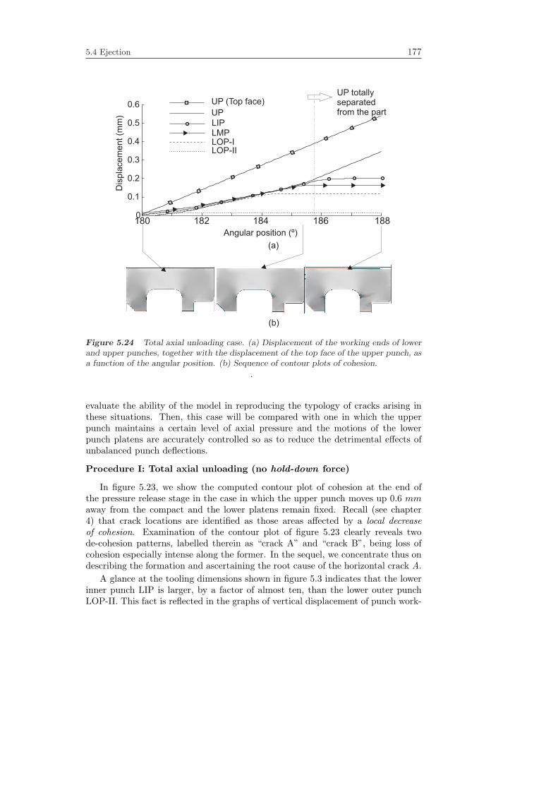
5.4 Ejection 177
0
0.1
0.2
0.3
0.4
0.5
0.6
LIPLMPLOP-ILOP-II
UP
UP (Top face)
(b)
(a)
UP totallyseparatedfrom the part
Angular position (º)
Dis
pla
ce
me
nt
(mm
)
180 182 184 186 188
Figure 5.24 Total axial unloading case. (a) Displacement of the working ends of lowerand upper punches, together with the displacement of the top face of the upper punch, asa function of the angular position. (b) Sequence of contour plots of cohesion.
.
evaluate the ability of the model in reproducing the typology of cracks arising inthese situations. Then, this case will be compared with one in which the upperpunch maintains a certain level of axial pressure and the motions of the lowerpunch platens are accurately controlled so as to reduce the detrimental effects ofunbalanced punch deflections.
Procedure I: Total axial unloading (no hold-down force)
In figure 5.23, we show the computed contour plot of cohesion at the end ofthe pressure release stage in the case in which the upper punch moves up 0.6 mmaway from the compact and the lower platens remain fixed. Recall (see chapter4) that crack locations are identified as those areas affected by a local decreaseof cohesion. Examination of the contour plot of figure 5.23 clearly reveals twode-cohesion patterns, labelled therein as “crack A” and “crack B”, being loss ofcohesion especially intense along the former. In the sequel, we concentrate thus ondescribing the formation and ascertaining the root cause of the horizontal crack A.
A glance at the tooling dimensions shown in figure 5.3 indicates that the lowerinner punch LIP is larger, by a factor of almost ten, than the lower outer punchLOP-II. This fact is reflected in the graphs of vertical displacement of punch work-

178 5. Modeling guidelines for industrial applications: compaction of a multilevel part
-250 -200 -150 -100 -50 0
Cauchy mean stress, Mpa
50
100
150
200
250
0
Cauchy d
evia
toric s
tress, M
pa
A
B
C
D
Figure 5.25 Stress trajectory in the mean-deviatoric plane at a point located in thearea affected by the de-cohesion pattern labelled as “Crack A” in figure 5.23.
.
ing ends versus the angular position contained in figure 5.24.a. The LIP experiencesthe greatest total deflection - approximately 0.2 mm -, in contrast to the almostnegligible change in dimensions of the lower outer punch LOP-II. This means thatthe compact moves with the lower inner punch and, consequently gaps are gen-erated between the working ends of the lower outer punches and the compact, ascan be observed in figure 5.23. In this process, the outer flange is partially grippedbetween the LMP outer wall and the LIP-I inner wall, due to friction effects. Thecombination of this restraining action and the upward movement of the LIP placesin tension the corner region and the crack is therefore induced. The propagationof this crack can be visualized in the sequence of cohesion contours displayed infigure 5.24.b.
In order to corroborate the physical origin of this de-cohesion pattern, the stresshistory at a point located in the affected area is plotted in the mean-deviatoricstress plane (see figure 5.25). The stress state at the beginning of axial unloading islocated at point A. As axial unloading progresses, it moves toward the tensile region(first quadrant) following the path ABC (elastic regime). At point C, however, itencounters the Drucker-Prager failure line, which represents the limited ability ofthe green compact to resist tensile stresses. Continued strain (of tensile nature),provoked by the aforementioned uneven tooling deflection, induces continued plasticyielding and thus a local decrease of cohesion (strain softening), causing the stressstate to travel along the failure line towards the origin (point D). No anomalousoscillations, due for instance to an unsatisfactory reproduction of the tool-powdercontact behavior, are observed. This indicates that numerical flaws do not pollutethe response, and, therefore, the de-cohesion pattern can be ascribed definitely tothe aforementioned mechanical cause.

5.4 Ejection 179
Procedure II: Balanced deflection of lower punches ( with hold-downforce)
The foregoing scenario represents working conditions quite similar to that en-countered in press machines whose upper rams are actuated exclusively by mecha-nical drives. One of the major disadvantages of those presses is the sudden releaseof force occurring after the rotating drive member reaches the bottom dead center(ϕ = 180). However, we mentioned earlier that the analyzed part was manufac-tured in a press machine in which, during the post-pressing operations, the upperpunch is operated by a separate hydraulically drive system. This mechanism allowsto apply a certain downward pressure during withdrawal of the die, the so-calledhold down or counter- pressure. In the numerical simulation presented in the fol-lowing, the upper punch is gradually lifted until the axial force on the upper punchis set to 10 Tons. The CNC press machines also offers the possibility of accu-
Angular position (º)
Dis
pla
cem
ent (m
m)
180 182 184 186 188 190 192-0.05
0
0.05
0.1
0.15
0.2
0.25LIPLMPLOP-ILOP-II
UP
UP (Top face)
Figure 5.26 Balanced deflection of lower punches case (hold-down force). Displacementof the working ends of lower punches, as well as the displacement of the top face of theupper punch, as a function of the angular position.
.
rately controlling the position of the lower rams. In order to compensate for theunbalanced punch deflections, the lower inner punch LIP, which is the largest one,descends 0.05 mm, whereas the lower outer punch LOP-I moves 0.04 mm upward.The LMP and die platens are kept fixed. Figure 5.26 displays the computed verti-cal displacement, as a function of the angular position, of the punch working endstogether with the displacement of the top face of the upper punch. According tothe graph corresponding to the UP top face, the imposed reduction in axial forcerequires to move the upper punch 0.25 mm upward. The displacement curves cor-responding to the working ends of the UP, LIP, and LMP-I meet at the end ofthe pressure release stage, a fact that indicates that the motions prescribed at thebottom of the LIP and LMP-I have proved efficient in compensating for the differ-ences in elastic deflection between punches. The relative uniformity exhibited bythe cohesion distribution computed at the end of pressure release stage, displayed

180 5. Modeling guidelines for industrial applications: compaction of a multilevel part
UP
COREROD
LOP-II
LOP-I
LMP
LIP
Cohesion (Mpa)
Figure 5.27 Contour plot of cohesion at the end of pressure release stage. Balanceddeflection of lower punches case.
.
in figure 5.27, confirms also this efficiency since, in contrast to the contour plotcomputed in the previous situation of uncontrolled punch deflection (figure 5.23),no appreciable evidences of loss of cohesion are detected.
5.4.0.2 Withdrawal of the die
Using as starting point the results obtained at the end of the pressure release stage,we tackle now the analysis of the die withdrawal phase. Three different ejectionprocedures are numerically tested. In these three alternatives, the compact is heldbetween the upper punch and the two lower punches forming the lowest faces ofthe compact (LIP and LOP-I), which act, thus, as supporting punches as the dieis withdrawn.
Option a: Held stationary the LMP and the core rod.
We shall explore first the consequences of keeping fixed the lower middle punchand the core rod as the die is lowered. The tooling motion profile corresponding tothis situation is depicted in figure 5.28. This diagram is accompanied by a sequenceof three contour plots of cohesion computed at different times during the process.In the rightmost plot, which is shown also - in magnified form - in figure 5.29.a,a horizontal de-cohesion path stemming from the outer wall is observed. This de-cohesion pattern certainly exhibits a distinctly crack-like appearance. However,the factor or factors that provoke its development are not readily apparent. Inorder to identify these factors, and eventually clarify the physical origin, if any, ofthis localized loss of cohesion, we shall propose two alternative, physically plausiblehypothesis.
The first hypothesis considers that the computed crack is due to the effects ofelastic strain release in the radial direction. The observed mechanical degradationarises when the top face of the die is approximately flush with the top face of the

5.4 Ejection 181
LIPLMPLOP-ILOP-II (DIE)
CORE ROD
UP
180 190 200 210 220 230 240 250 260 270-15
-10
-5
0
5
10
15
Angular position (º)
Dis
pla
cem
ent (m
m)
Figure 5.28 Prescribed punch displacements as a function of the angular position,together with a sequence of contour plots of computed cohesion. Case in which the LMPand the core rod are held stationary.
.
lower middle punch, that is, when the main body of the part is clear of the die.The radial expansion of the main body coupled with the radial force exerted onthe portion of outer surface still restrained by the die tends to shear the compactalong the radial direction, as pictorially depicted in figure 5.29.b. Accordingly,this presumably shear-mode (or mode-II ) crack can be eliminated by reducing thelevel of radial stress when withdrawing the die. One possibility to carry out thisreduction is, as recommended by Zenger et al. [112], to decrease the degree ofconfinement of the part by withdrawing the lower middle punch and the core rod.Another possibility to reduce the effects of radial expansion would be to diminishthe hold down pressure exerted by the upper punch. However, this practice mayconflict with the requirements for avoiding the crack promoting effect, describedpreviously, of uncontrolled punch deflections.
The other hypothesis advocates that the root cause of the numerically pre-dicted crack is the “stepped” character of the die. As already mentioned, the lowerouter punch LOP-II is mounted on the die platen. Thus, as the die descends tofree the part, the LOP-II inevitably moves down away from the compact. Thisseparation leaves the external portion of the compact vertically unsupported and,consequently, frictional downward forces between the die and the compact may tend

182 5. Modeling guidelines for industrial applications: compaction of a multilevel part
Cohesion (Mpa)
CORE ROD
UP
LIP
LMPLOP-I
(a)
(b)
DIE
Expansiondue toelastic strainrelease
Figure 5.29 (a) Contour plot of computed cohesion at φ = 203 for the case in whichthe LMP and the core rod are held stationary. (b) Schematic representation of the effectof elastic strain release.
.
to pull apart the main body and the bottom section. According to this hypothesis,thus, the horizontal crack develops predominantly under opening or mode-I load-ing conditions. In turn, the bending deformation caused by these frictional forceswould also explain consistently the formation of the other discernable de-cohesionpath (see figure 5.29.a), located at the top face of the part.
In order to ascertain which hypothesis is more consistent, we shall carry out twoadditional finite element analysis of the die withdrawal stage. In the first one, thelower middle punch and the core rod accompany the die in its downward motionso as to release some elastic radial strain. In the second one, the lower inner punchis kept fixed so that it can support the part while the die descends.
Option b: Withdrawing the core rod and the LPM simultaneously
The tooling displacement diagram, together with a sequence of three contourplots of cohesion, corresponding to this case are shown in figure 5.30. For easeof visualization, an enlarged view of the contour plot at ϕ = 230 is displayedin figure 5.31.a. Details of crack propagation through the mesh employed in thecalculations can be appreciated in figure 5.31.b. A qualitative comparison of thecontour plot in figure 5.31.a with that contained in figure 5.29 leads immediatelyto the conclusion that withdrawing the lower middle punch and the core rod hasnot proved effective in eliminating the observed cracks. Both contour plots exhibitsthe same de-cohesion patterns, being the only discernable effect a slight decrease

5.4 Ejection 183
LIPLMPLOP-ILOP-II (DIE)
CORE ROD
UP
180 190 200 210 220 230 240 250 260 270-15
-10
-5
0
5
10
15
Angular position (º)
Dis
pla
cem
ent (m
m)
Figure 5.30 Prescribed punch displacements as a function of the angular position,together with a sequence of contour plots of computed cohesion. Case in which the LMPand the core rod are withdrawn simultaneously with the die.
.
(b)(a)
Cohesion (Mpa)
Figure 5.31 (a) Contour plot of computed cohesion at φ = 230. Case in which theLMP and the core rod are withdrawn simultaneously with the die. for the kinematicsshown in figure 5.28, for φ = 230. (b) The same contour plot showing the mesh used inthe computations.
in the intensity of the degradation along these paths.
Option c: Holding stationary the LOP-II.
The modeling of this scenario requires to consider a tooling arrangement diffe-rent from the one described in section 5.2. Rather than attached to the die platen,

184 5. Modeling guidelines for industrial applications: compaction of a multilevel part
LIPLMPLOP-I
LOP-II
CORE ROD
UP
Angular position (º)
Dis
pla
cem
ent (m
m)
180 190 200 210 220 230 240 250 260 270-20
-15
-10
-5
0
5
10
15
DIE
Figure 5.32 Prescribed punch displacements as a function of the angular position,together with a sequence of contour plots of computed cohesion. Case in which theLOP-II moves independently from the die.
the LOP-II is assumed to be mounted on an independent platen so that it cansupport the compact during the downward motion of the die platen. Consequently,in this ejection schedule the part is fully supported by the four lower punches, asindicated in the diagram of tooling displacements shown in figure 5.32. Below thisdiagram we show the cohesion distribution at three different times during the diewithdrawal. The central plot depicts a situation in which the top face of the die ispractically flush with the working end of the LMP, which is the relative positionof die and LMP at which the de-cohesion patterns reported in the preceding simu-lations were detected. In this case, by contrast, the cohesion distribution exhibitsa relatively uniform aspect and no evidence of intense loss of cohesion is observed.This fact clearly substantiates the second hypothesis advanced previously. Thus,we can conclude from the numerical simulations carried out that the root causeof the numerically predicted cracks (shown in figure 5.29.a) lies in the “stepped”character of the die.
Incidentally, examination of the rightmost contour plot in figure 5.32 (displayedin magnified form in figure 5.33.a) shows a vertical, slightly leaned inwards, de-cohesion path that develops at the junction between the levels formed by the LOP-Iand the LOP-II. Although the primary goal in studying this ejection schedule wasto merely confront the hypothesis advanced at the onset of the discussion, ratherthan rigorously investigate the defects formed in producing the part using this

5.4 Ejection 185
Cohesion (Mpa)
(b) (c ) (d )
(a)
F
DIELOP-II
Figure 5.33 (a) Contour plot of computed cohesion at ϕ = 226. Case in which theLOP-II moves independently from the die. (b) (c) Enlarged views of the zone at whichthe crack is formed (d) Schematic representation of the force generated on the protrudingrim due to radial expansion.
tooling arrangement13, it may prove instructive to, at least superficially, inquireabout the root cause of this de-cohesion pattern.
A plausible explanation for this localized loss of cohesion may lie in the partic-ular geometry of the LOP-II. Inspection of the plots in figures 5.33.b and 5.33.cindicates that loss of cohesion in the corner region occurs right after the compactis totally freed from the radial restraint imposed by the die. The top surface of theLOP-II is not completely horizontal, but it has a vertical protruding feature (0.2mm height, see figure 5.1) at the outer edge. As the compact emerges from thedie, it tends to expand radially due to elastic strain release. The radial expansionof the lower portion of the part, however, is hindered to some extent by the pro-truding feature. This restriction generates a lifting force (see figure 5.33.d), that,considering that the leg section is restrained by the radial action of the LOP-II andthe LMP, induces bending of the part. The computed de-cohesion path might beascribed thus to the effects of such bending deformation.

186 5. Modeling guidelines for industrial applications: compaction of a multilevel part
23.34
24.16
28.14
36.8
39.78
44.759
0.9
2
R1 R1
Æ
Æ
Æ
Æ
Æ
Æ
0.15
5.3
22
±0
.09
2.7
±0
.1
0.4
2±
0.0
2
42Æ
Revised geometry
Old geometry
Figure 5.34 Revised geometry (dimensions in mm).
5.4.1 Revised design
Figure 5.34 shows the revised design of the part. The only modification with respectto the original design is that the difference in length between the levels previouslyformed by the LOP-I and LOP-II has been diminished considerably. Furthermore,a tapered surface has eliminated the abruptness of the cross-sectional change. Themain implication of this geometry modification is that it dispenses with the needfor two separate lower outer punches. Accordingly, the two thin-walled lower outerpunches LOP-I and LOP-II employed in shaping the part in its original conceptionare replaced by a single, more massive, lower outer punch, abbreviated LOP, witha tapered top surface. Observe that this modification is totally consistent withthe hypothesis put forward in the previous section for explaining the difficulties inproducing a free-defect part using the “stepped die” tooling configuration.
UP LIP LMP LOP DIE CORE RODf 1 0.043 0.234 0.019 0.173 0.233
Table 5.10 Motion scale factors used for pressing the modified part.
The pressing kinematics is defined by the motion scale factors tabulated intable 5.10. The determination of the starting conditions and the analysis of thepressing stage proceed along the same lines described in section 5.3.1. We bypassthus such details and concentrate exclusively on presenting the computed resultscorresponding to the ejection stage.
13In practice, this tooling arrangement with an independently movable LOP-II was not testeddue to equipment limitations.

5.4 Ejection 187
Procedure I: Total axial unloading (no hold-down force)
In order to evaluate again the ability of the model in reproducing the typology ofcracks arising in situations of unbalanced punch deflections, we consider first a casein which the upper punch moves up away from the compact and the lower platensremain fixed. In figure 5.36, the graphs of the computed displacement of punchworking ends versus the angular position are displayed. Below this diagram, weshow a sequence of contour plots of computed cohesion. A horizontal de-cohesionpath emanating from the junction corner and propagating outwards through thesection change is easily detected in these plots.
180 181 182 183 184 1850
0.05
0.1
0.15
0.2
0.25
0.3
0.35
0.4
LIP LMP LOP
UP
UP
UP (Top face)LIP
LOP
LMP
Angular position (º)
Dis
pla
cem
ent (m
m)
gap
Figure 5.35 Total axial unloading case (modified part). (a) Displacement of the workingends of lower and upper punches, together with the displacement of the top face of theupper punch, as a function of the angular position. (b) Sequence of contour plots ofcohesion.
.
The reasoning behind this localized mechanical degradation is essentially thesame outlined in section 5.4.0.1 for explaining the formation of the de-cohesionpattern labelled as “Crack A” (see figure 5.23). In this case, however, crackingis markedly more intense that in the one shown previously in figure 5.23. At theend of the pressure release stage (see figure 5.36), the computed de-cohesion pathspans the whole section, a fact that suggests that fracture is imminent. This canbe readily explained from the punch displacement diagram displayed in figure 5.36.The difference between the deflections experienced by the lower inner punch andthe lower outer punch in compressing the modified part is more pronounced that inthe original part case (see figure 5.24, curves LIP, LOP-I), due to the greater cross-

188 5. Modeling guidelines for industrial applications: compaction of a multilevel part
Cohesion (Mpa)
Figure 5.36 Contour plot of cohesion at the end of pressure release stage. Total axialunloading case (modified part)
.
sectional area of the LOP in comparison to the LOP-I. Bending deformation istherefore accentuated, and this results, in turn, in an intensification of the crackingprocess.
Procedure II: Balanced deflection of lower punches (with hold-downforce)
We carry out now the finite element analysis of a pressure release stage inwhich the lower outer punch and the lower middle punch are programmed to moveupward 0.08 mm and 0.06 mm while maintaining a hold down force of 10 Tons.Figure 5.37 shows the evolution of the computed displacement of the punch workingends. The curves corresponding to the lower punches gradually approach eachother, eventually meeting at ϕ = 192. This indicates that gaps between the lowerpunch ends and the compact have been eliminated. In addition, examination ofthe contour plot of cohesion displayed in figure 5.38 shows that the programmedpunch strokes have also proved effective in totally mitigating the crack reportedwhen studying the unbalanced deflection case (figure 5.36).
The conditions computed at the end of the above presented pressure releasestage are used as starting conditions for simulating the rest of the ejection process.The tooling motions according to which the part was finally manufactured aredisplayed in figure 5.39. First the die is lowered so as to free the part. Thedownward motion of the die is followed by the withdrawal of the core rod and thelower middle punch. Finally, the upper punch moves up away from the compactand the lower inner punch is slightly lifted so as to ready the part for being removedby the gripper. The cohesion distribution computed at four different positions are

5.5 Conclusions 189
UP
UP
UP (Top face)LIP
LOP
LMP
Angular position (º)
Dis
pla
cem
ent (m
m)
180 182 184 186 188 190 1920
0.1
0.2
0.3
0.4
Figure 5.37 Balanced deflection of lower punches case (modified part). (a) Displace-ment of the working ends of lower and upper punches, together with the displacement ofthe top face of the upper punch, as a function of the angular position.
Cohesion (Mpa)
Figure 5.38 Contour plot of cohesion at the end of pressure release stage. Balanceddeflection of lower punches case (modified part).
shown also in figure 5.39. It is apparent that the cohesion field remains unaffectedduring the ejection process. The model predictions, therefore, are in accordance withexperimental evidence and confirm the benefits of manufacturing the part accordingto the revised design.
5.5 Conclusions
This chapter was devoted to discuss several aspects concerning the numerical sim-ulation of the compaction of an axisymmetric multilevel part in an advanced CNC

190 5. Modeling guidelines for industrial applications: compaction of a multilevel part
180 190 200 210 220 230 240 250 260-20
-15
-10
-5
0
5
10
Angular position (º)
Dis
pla
cem
ent (m
m)
LIPLMP
UP
LOP
CORE ROD
DIE
Figure 5.39 Prescribed punch displacements as a function of the angular position,together with a sequence of contour plots of computed cohesion (modified part).
press machine. Emphasis on the first part of the chapter was placed on conveyingthe relevance of an accurate characterization of the tooling set and the externalactions acting on it if one whishes to obtain a satisfactory computed response. Itwas shown that numerical predictions of density distributions using, as prescribedconditions on tools, theoretical or nominal motions can result in substantial dis-agreement with experimental measurements. It is therefore essential to possess aproper knowledge on the CNC press performance so as to be aware of potentialsources of deviations from nominal tooling motions. Unawareness of such factorsmay promote the tendency of rationalizing discrepancies as being due to flaws ei-ther in the constitutive model or in the algorithmic procedure used to computethe response and, thus, one would be tempted in this case to either refine the con-stitutive equation or to increase the accuracy of the approximation so as to bringnumerical predictions into agreement with experimental values. But one does notincrease the strength of a chain by improving the strong links. Further refinementsof these aspects of the model would be in vain, and rather than embarking on thesemathematically and computationally challenging research efforts, one should con-centrate task of revising the available input data and the characterization of thetool set.

5.5 Conclusions 191
An aspect that has also received special consideration is that of the optimizationof the pressing sequence. It was shown that the problem can be posed mathemat-ically as a nonlinear constrained optimization problem. It was argued that thesolution of this problem can be approximated by the solution of a similar problemdefined in terms of density predictions provided by an elementary “column model”.The validity of this statement was assessed by a finite element simulation, whichfinally corroborated the optimum character of the pressing route calculated on thebasis of the elementary column model. As explained, in instances in which frictioneffects play a dominant role in determining density gradients, this column model-based procedure may fail in determining a pressing sequence close to the “ideal”tooling motion. Therefore, caution is required in extending this methodology tothe design of parts of considerable height.
To date, the modeling of the pressing stage and the densification phenomenonhave been the focus of the vast majority of research efforts in the field. Boththe abovementioned assessment of the impact of accurately representing the toolset and the external actions and the determination of optimum tooling motionwere carried out in terms of density values attained at the end of the pressingstage, and hence, they are essentially further contributions to this research aspect.By contrast, the analysis of the formation of cracks during the ejection stage liesoutside the scope of conventional finite elements studies of the compaction process,and can be considered thereby as an original and innovative part of this chapter.
Observations made in this study are in qualitative agreement with experimentalevidences. The absence of easily discernable de-cohesion patterns in the cohesiondistribution computed at the end of the ejection phase - in the modified part case,see figure 5.39-, provides convincing proof of the consistency of the computed re-sults. Numerical simulation of several ejection routes have illustrated the difficultiesencountered in manufacturing the part according to the original design. Scrutiny ofthe computed cohesion distributions resulting from such simulations have allowedus to give physically plausible reasons for explaining such difficulties.
The overall impression gained is that the judicious interpretation of cohesiondistributions predicted by the model can provide satisfactory answers to practicalquestions related to the design of an adequate ejection route. However, this is notintended to suggest that the model can predict with certainty, in any circumstances,the formation and development of cracks. In principle, the numerical simulationof a given ejection route attempts to answer the question: will this ejection routelead to a free-defect part ? But such a question demands a categorical yes orno answer; there is no flexibility and the risk of arriving at wrong conclusionsis thus high. Except in some pathological cases, such as the uncontrolled punchdeflections (see figures 5.23 and 5.36), we should theferore refrain from drawingdefinite conclusions from a single simulation. A more fruitful strategy consists inrunning several analysis for different alternative ejection procedures, and limitingourserlves to answer the question: which of these ejection procedures representsmore favorable conditions for ejecting the part safely from the die? The case studypresented in this chapter has demonstrated that this question can be consistentlyanswered by our approach.

192 5. Modeling guidelines for industrial applications: compaction of a multilevel part
The advantages of employing FE simulations of the ejection process becomesespecially apparent when alternative tooling arrangements are to be tested. Designand manufacturing of the new tooling, together with the changeover of the die set,are time-consuming and costly tasks. Prior to undertaking these operations, severalFEM analysis can be performed to evaluate the feasibility of the operation.
The capacity to predict crack formation and its implication at the design stageare not the only issues to be considered when using the numerical model. Normally,the definite sequence of ejection is achieved by trial-and-error procedures guidedby the operator’s intuitive experience. This means the that the “how” is finallyin hands of the operator. But intuition is difficult to characterize if the “how” isachieved without a mechanically grounded understanding of the “why”. Numer-ical simulations can serve the useful purpose of clarifying the reason behind theappropriateness of the ejection route empirically found, so as to establish practicalrecommendations that will facilitate the ejection of similar parts. Last but notleast, numerical FEM simulations have the added benefit of illustrating the pro-cess by attractive graphics. The visualization of cracks as de-cohesion patterns isparticularly appealing, since it does not require a profound knowledge on the math-ematical basis of the model. Computed displaced shape displayed in conjunctionwith contour plots of cohesion may be of considerable assistance in both fuelingthe interest of uninitiated practitioners and stimulating the intuition of experiencedPM technologists.

Chapter 6
Concluding remarks
The primary goal of this work was to explore the possibilities of numerically sim-ulating crack formation during the post-pressing stages in uniaxial die compactionprocesses. A phenomenological approach was adopted to mathematically representthe behavior of our target system, which comprises both the powder contained inthe die cavity and the tooling employed to consolidate the powder into the finalshape. Research effort has been focused on constructing a large strain elasto-plasticconstitutive model able to describe, in an unified manner, both the densification ofthe powder under compressive stress states and the formation of cracks during thepost-pressing operations. The innovative part of our modeling is mainly connectedwith the characterization of the latter phenomenological aspect, i.e: cracking.
6.1 On the general features of the proposed con-stitutive model
For the purpose of modeling the material behavior in stress space, the elastic do-main is bounded by three surfaces intersecting non-smoothly, namely, an ellip-tical cap -associated with hardening behavior-, and two classical Von Mises andDrucker-Prager yield surfaces. The truly original feature of the formulation isthe use of a parabolic plastic potential function to describe the plastic flow on theDrucker-Prager failure surface. The introduction of this non-classical plastic po-tential function has proved successful in reproducing the experimentally observedplastic isochoric behavior in the shear regime, while avoiding the acclaimed nu-merical shortcomings appearing when jointly using traditional pure isochoric flowrules and implicit integration procedures. However, the constitutive implicationsof the practically pure dilatational deformation occurring when the updated stressstate lies close to the vertex of the Drucker-Prager has not been fully explored.To further improve the confidence in the proposed constitutive model, this aspectshould be subjected to close scrutiny in future developments.
193

194 6. Concluding remarks
6.1.1 The fracture modeling
A classical strain localization approach has been adopted for modeling the crackingphenomenon. Incorporation of a softening law - relating cohesion and accumu-lated plastic shear strain - permits the representation of macroscopic cracks as highgradients of inelastic strains concentrated along bands of finite thickness. In turn, anovel, thermodynamically consistent calibration procedure has been used to relatematerial parameters involved in this softening law to fracture energy values ob-tained experimentally on Distaloy AE specimens. The convergence studies carriedout in dealing with the Brazilian test case indicates that the proposed regularizationof the softening law, although not very elaborated, seems to alleviate the problemof lack of convergence upon refinement of the finite element mesh. The other mainfactor that rendered the choice of a classical strain localization approach objection-able is the mesh-induced directional bias of the computed cracks - the propagatinglocalization band tends to follow certain preferred directions dictated by the mesh.However, it was argued that this criticism is blunted if viewed in the light of theaim and purpose of our investigation. Our primary concern was to capture anyevidence of macroscopic cracking, but without a compelling necessity of giving anaccurate and detailed description of the crack growth conditions. In this respect,results presented in chapters 4 and 5 have certainly demonstrated the ability of themodel in revealing evidence of macroscopic defects and in qualitatively evaluatingthe influence, in the formation of cracks, of variations in the input data (materialparameters, tooling kinematics, etc). A more realistic representation of the physicaldiscontinuity would require to abandon this elementary approach in favor of one thevarious sophisticated - viz. more complex -, material failure modeling techniquesthat have, in recent years, successfully superseded the smeared crack approach inother fields of solid mechanics. Such refinements will be fruitless, however, unlessother more elementary aspects of the model, equally relevant to the accuracy ofthe predictions, are also improved. Accordingly, moving to more sophisticated ap-proaches for representing the cracking process is not regarded as a priority, at leastin the short term.
6.1.2 The thermodynamic framework
Although certainly not an original contribution of this work, the mathematicalform of the constitutive relationships describing the other phenomenological as-pects - elastic and hardening behavior - has been derived with the same rigor andcare as the softening law. In fact, one of the distinguishing features of this work isthat the formulation of the constitutive model is entirely cast within a rational ther-modynamic framework. The foremost motivation in such a thermodynamic sound-ness was to originate our considerations from the most general standpoint possible,with a view towards future extensions of the model. For example, the paucity ofexperimental results concerning fracture energy compelled us to make some restric-tive assumptions and eventually consider only one internal variable for capturingthe softening behavior of the green compact. One internal variable may appeartoo simplistic for accounting for the effects of the whole range of micromechani-

6.2 On the integration of the constitutive equation 195
cal events occurring at the damage zone. Consequently, flaws in these restrictiveassumptions may be uncovered as more experimental data become available, andthis may dictate the eventual incorporation of additional internal variables. Thethermodynamically consistent structure of the constitutive equation will facilitateconsiderably the seamless accommodation in the model of these new variables.
Another motivation was to ensure the satisfaction of the second law of the ther-modynamics, an aspect often disregarded by many researchers in the field. Com-patibility with the second law does not imply that the response predicted by ourmodel is in closer agreement with experimental observations than responses com-puted using other models not embedded in a thermodynamic framework, but ratherprovides the confidence that thermodynamically unreasonable results -“negativedissipation” - are not produced in loading situations different from that used forcalibrating the model. The demonstration of the consistency of the proposed con-stitutive model with the second law of thermodynamics, carried out in appendixC, can be considered also as an original contribution of this work.
6.2 On the integration of the constitutive equation
Due to the presence of strain softening and the non-linear, tightly coupled characterof the governing equations, standard procedures turned out to be inadequate forcarrying out the (implicit) numerical integration of the constitutive equation, andwe were thus compelled to develop an alternative, apparently novel, method fordealing with this problem. The proposed local integration procedure has the intu-itive flavor of a fractional step method (FSM), since it is based on the decouplingof the evolution equations for the the plastic strains and the internal variables.The algorithmic structure underlying this methodology has been discussed in athorough manner, placing special emphasis on the issues of convergence and exis-tence of solution. In particular, it has been shown that the solution of the return-mapping algorithm has an unique solution for any conceivable stress state trial.Another remarkable feature is that plastic consistency is restored in a maximumof three iterations of the FSM predictor-corrector scheme, except when the trialstress is projected onto the Drucker-Prager yield surface. In this case, nevertheless,it has been rigorously proved that the sequence defined by the predictor-correctorscheme converges unconditionally to the solution, with a linear rate of convergence.Concerning the global iteration scheme, the introduction of the IMPLEX (implicit-explicit) integration procedure has proved crucial in avoiding the adverse effects ofsoftening-induced non-positive definite algorithmic elastoplastic moduli, exhibitedtypically by purely implicit, standard integration schemes. Furthermore, it has be-come evident that, if used in conjunction with an adequate adaptive time steppingscheme, the IMPLEX procedure offers an efficient solution to the trade-off betweenrobustness and computational time requirements.

196 6. Concluding remarks
6.3 On the robustness of the solution algorithm
Numerical experience indicates that the main cause of convergence difficulties isthe inaccurate computation of the powder-tooling contact response. Too largetime steps, an inadequate mesh, specially at regions of stress concentration, or thecombination of these two factors may imply a poor enforcement of the impenetrabil-ity constraint. Small amounts of interpenetration can be tolerated without seriousconsequences in the compression regime (pressing stage). By contrast, contactinaccuracies are particularly detrimental under tensile stress conditions (ejectionstage). The synergistic combination of the effects of innacuracies in computingthe contact response and the dilatational deformation associated to stress stateslying close to the apex of the Drucker-Prager yield surface induces severe distor-sion of the mesh at the boundary of the powder body, with consequent negativeimpact on the performance of the global algorithm. This fact dictated the choice ofthe more computationally costly -in comparison with the penalty approach- aug-mented lagranian strategy for computing the contact response in the simulation ofthe ejection process.
6.4 On the simulation technology
The numerical simulation of the compaction of an axisymmetric multilevel part inan advanced CNC press machine has enabled us to appreciate the extreme impor-tance of accurately characterizing the geometry of the tool set and the externalactions acting on it. Although the assessment of the effect of the innacurate repre-sentation of tooling motions was carried out in terms of final density distributions-cracking is not a readily quantifiable phenomenon-, similar considerations applyto the simulation of the formation of cracks during the ejection stage. One shouldregard, accordingly, the problem from a broader perspective, more in concordancewith the systemic conception adopted in this work, and not remain exclusivelywithin the confines of powder constitutive modeling, since discrepancies betweenobserved and calculated responses may be attributable to an inadequate model-ing of the tooling sub-system and the environmental actions, rather than in anunsatisfactory representation of the powder behavior.
The multilevel part case-study has served also to exemplify the use of the modelas a tool for supporting and guiding - but never supplanting - engineer judgementin a practical problem. It has become apparent that the judicious interpretationof cohesion distributions can considerably assist in understanding the underlyingphysical mechanisms that control the occurrence of cracks during the ejection pro-cess. Useful insight can be squeezed from simple qualitative comparisons of cohe-sion contours obtained from simulation of alternative ejection routes. The proposedcomputational model is certainly not perfect, as no engineering analysis is, and itmay fail in answering some practical questions. But, as clearly evidenced through-out this work, it can provide satisfactory answers to many others, which is, in ouropinion, sufficient justification for its use.

Appendix A
Mathematical aspects of thecontinuum formulation
A.1 Large strain kinematics
We regard the powder sub-system as a deformable body B consisting of continuouslydistributed material occupying, at a reference time t0, a region Ω0 of Rn (n = 2, 3).As is customary, we designate the position vector X, with respect to a fixed originO, of the particle X ∈ B in the reference configuration Ω0 as the label of thisparticle throughout the deformation process. We assume that the deformation attime t relative to the reference configuration is given by the one-to-one C2 mapping
ϕ : Ω0 → Ωt ⊂ Rn. (A.1.1)
Hence, we can write the position vector, with respect to a fixed origin o, of particleX ∈ B in the so-called current configuration Ωt as
x = ϕ (X, t) . (A.1.2)
We introduce a coordinate system in the reference configuration Ω0, defined byits origin 0 and a set of orthogonal basis vectors EA (A = 1, 2, 3), and anothercoordinate system in the current configuration Ωt, with its origin in o and orthog-onal basis vectors ea, (a = 1, 2, 3). Thus, it can be written X = XAEA andx = xaea 1, where the summation convention for two repeated indices holds.
A line element dX placed on point X in Ω0 transforms into a line element dxplaced on x in Ωt according to the linear mapping2
dx = F (X, t)·dX. (A.1.3)1Convention index used throughout this appendix follows Marsden and Hughes [63]. Upper
case letters refer to the reference configuration Ω0 and lower case for the current configurationΩt. Index placement (superindex and subindex) will be discussed later.
2More precisely, F is a linear mapping from the tangent space of Ω0 at X to the tangent spaceof Ωt at x, i.e. F : TX(Ω0) → Tx(Ωt) [73, 63].
197

198 A. Mathematical aspects of the continuum formulation
The second-order tensor F(X, t) is called the deformation gradient of ϕ [63],and it can be defined, in abstract form, as
F (X, t) =∂ϕ (X, t)∂X
, (A.1.4)
or through its components along the basis vectors EA and ea as
F aA(X, t) =∂ϕa(X, t)∂XA
. (A.1.5)
Impenetrability of matter, i.e. no two particles can occupy the same place in spaceat a given time, requires J = det(F) > 0. The gradient tensor F is, therefore, anon-singular second-order tensor and hence admits the local polar decomposition
F(X) = R(X)·U(X) = V(x)·R(X), (A.1.6)
where R(X) is an orthogonal rotation tensor and U(X) and V(x) are symmetricpositive-definite stretch tensors. The so-called right Cauchy-Green tensor is definedas
C(X) = FT(ϕ (X))·F (X) = (R(X)·U(X))T ·R(X)·U(X) = U2(X), (A.1.7)
or in component form (omitting explicit indication of the argument)
CAB = gabFaAF
bB , (A.1.8)
where gab is the matrix of the metric tensor associated with the inner product in thespatial configuration Ωt. Since we are using cartesian coordinates system, we havegab = δab, being δab the second-order Kronecker delta. In fact, the placement ofthe suffix (superscript or subscript) is irrelevant for the value of tensor componentsin the setting of a cartesian representation (e.g., F aA = FaA = F aA). However, inorder to distinguish the covariant and contra-variant character of tensors, we shallattempt to keep the natural position of indices of tensor components. Therefore,Eq.(A.1.8) indicates that the right Cauchy-Green tensor C with components CABis a covariant tensor (of rank 2)3.
We shall employ as material strain measure the Green-Lagrange strain tensor,defined in the reference configuration Ω0 as
E(X) =12
(C(X)−G (X)) or EAB =12
(CAB −GAB) . (A.1.9)
3In a general coordinate system, the right Cauchy-Green tensor defined by C = FTF can beregarded as a linear mapping C : TX(Ω0) → TX(Ω0), with component representation CAB . The
associated tensor [63] of C is a covariant tensor C[ : TX(Ω0) → T ∗X(Ω0) (T ∗X(Ω0) is the dual space
of TX(Ω0)) with components CAB = GCACCB , GCA being the matrix of the metric tensor in Ω0.
Thus, rigorously speaking, components defined in Eq.(A.1.5) corresponds to C[ rather than to C.We make no such a distinction herein and assume that all strain tensors are covariant tensors.
A.1 Large strain kinematics 199
Note that for a local rigid motion C = G and therefore an unstrained state corre-sponds to E(X) = 0 . In analogous manner, the strained state is characterized inthe current configuration Ωt by the so-called Almansi strain tensor
e(x) =12
(g (x)− b-1(x)
), (A.1.10)
where b-1 is called the Finger deformation tensor, whose components are
(b-1)ab =(F-1
)Aa
(F-1
)BbGAB . (A.1.11)
Both e and b-1 are symmetric positive-definite covariant tensor defined in thecurrent configuration Ωt.
A remark concerning notation is in order here. Recall that G and g are themetric tensors in Ω0 and Ωt, respectively. Since both possess the same matrix rep-resentation in the setting of rectangular cartesian coordinates (the identity matrix),for simplicity in notation we often make g = 1 and G = 1, where 1 is the second-order identity tensor. Then, we can write E = 1
2 (C− 1) and e = 12 (1− b-1), with
the understanding that the object 1 has different meaning in each case. Likewise,the deformation gradient of a motionless body may be expressed as F = 1, being 1interpreted here as a two-point identity tensor relating Ω0 and Ωt. Index notationproves to be useful when ambiguity is to be removed (e.g. F aA = δaA ).
The push-forward and pull-back transformation induced by ϕ, which relatetensorial fields between both configurations [63], are denoted by ϕ∗(•) and ϕ∗(•),respectively. The components of the push-forward of a covariant4 second-ordertensor defined in Ω0 are given by
(ϕ∗ (•))ab =(F-1
)Aa
(F-1
)Bb(•)AB , (A.1.12)
or in direct notation5
ϕ∗(•) = F-T ·(•)·F-1, (A.1.13)
whereas the components of the pull-back of a covariant second-order tensor definedin Ωt can be written as
(ϕ∗ (•))AB = F aAFbB(•)ab, (A.1.14)
orϕ∗(•) = FT ·(•)·F. (A.1.15)
Therefore, in view of (A.1.8) and (A.1.11), the right Cauchy-Green tensor C and theFinger deformation tensor b-1 can be regarded as the pull-back of the metric tensor
4The definition of the operators ϕ∗(•) and ϕ∗(•) depends on their arguments. The pull-back,
for instance, of a contra-variant tensor in Ωt is defined as (ϕ∗ (•))AB =`F-1 A
a
`F-1 B
b(•)ab.
Since covariant indices can only contract with contra-variant indices, it can be established a rulefor defining ϕ∗(•) and ϕ∗(•) for tensors of any rank [63]. Roughly speaking, a covariant spatialindex, for instance, would transform into a covariant material index via FaA, i.e. T ......aF
aA = T ......A.
5Recasting the pull-back and push-forward operations in direct notation is a common practicein solid mechanics literature, and we also adopt it. However, we have to bear in mind that it lacksof any geometric sense (it is a consequence of the over-reliance on the cartesian structure, see Ref.[63]), and only definitions in component form Eq.(A.1.12) and Eq.(A.1.14) are strictly valid.

200 A. Mathematical aspects of the continuum formulation
in Ωt, C = ϕ∗(g), and the push-forward of the metric tensor in Ω0, b-1 = ϕ∗(G),respectively. Furthermore, it can be shown that the Almansi strain tensor is thespatial counterpart of the Green-Lagrange tensor
e = ϕ∗(E) or eab = (ϕ∗ (E))ab =(F-1
)Aa
(F-1
)BbEAB . (A.1.16)
The spatial velocity gradient l is a covariant second-order tensor defined by6
lab = gac∂vc
∂xb=
∂
∂t(∂xc
∂XB)∂XB
∂xb= gacF
cB
(F-1
)Bb, (A.1.17)
where vc denotes the components of the spatial velocity, or in abstract notation
l(x) = F(ϕ-1(x, t)
)F-1(x, t) , (A.1.18)
being F the derivative of F with respect to time holding X fixed. The spatialvelocity gradient is not a valid candidate for inclusion in the spatial description ofmotion due to the requirement of frame-indifference of any constitutive model [9].Nevertheless, its symmetric part, called the rate of deformation tensor
d(x) =12(l(x) + lT(x)), (A.1.19)
does conform with the definition of objective spatial tensor7.Furthermore, the rateof deformation tensor d can be interpreted as the Lie derivative8 of the Almansistrain tensor:
d = Lve = ϕ∗
(∂ϕ∗(e)∂t
)= ϕ∗
(∂E∂t
). (A.1.20)
A.1.0.1 Multiplicative decomposition
The standard local multiplicative decomposition of the deformation gradient intoplastic and elastic parts9 reads
F = Fe · Fp or F aA = (Fe)aA(Fp)AA. (A.1.21)
Although Fe and Fp cannot be considered as gradients of any deformation mapping,some kinematic relationship can be derived in analogy with the strain measuresgiven in Eq.(A.1.7), Eq.(A.1.9), Eq.(A.1.10) and Eq.(A.1.11). In the reference
6Following a frequent abuse of notation x = ϕ (X, t) = x (X, t) and X = ϕ-1(x, t) = X (x, t) .7d transforms according to d+ = QdQT under a superposed rigid body motion, defined by
the rotation tensor Q, of the spatial configuration.8Since tensor fields on the reference configuration remain unaltered under spatially superposed
rigid body motions, e is firstly pulled backward from the spatial to the reference configuration,yielding E, and then differentiated (E) prior to being pushed forward to the current configuration[63].
9To identify those tensorial fields associated to the intermediate configuration Ωt, we use a haton both the tensorial quantity and the corresponding index

A.1 Large strain kinematics 201
configuration Ω0, the plastic counterparts of the right Cauchy-Green tensor andthe Green-Lagrange tensor are defined as
Cp = FTp ·Fp or (Cp)AB = (Fp)AA(Fp)BBGAB , (A.1.22)
Ep =12(Cp − G) or (Ep)AB =
12
((Cp)AB −GAB) . (A.1.23)
where GAB = δAB is the metric defined in Ωt. Similarly, the elastic right Cauchy-Green Ce and Green-Lagrange Ee tensors, and the plastic Finger deformationand Almansi strain tensors, b
-1
p and ep, respectively, all of them defined in theintermediate configuration Ωt, are given by
Ce = FT
e ·Fe or (Ce)AB = (Fe)aA(Fe)bBgab, (A.1.24)
Ee =12(Ce − G) or (Ee)AB =
12((Ce)AB − GAB), (A.1.25)
b-1
p = F-T
p ·F-1
p or (b-1
p )AB = (F-1
p )AA(F
-1
p )BBGAB , (A.1.26)
ep =12(G− b
-1
p ) or (ep)AB =12(GAB − (b
-1
p )AB). (A.1.27)
Finally, the spatial elastic finger deformation tensor b-1e and the elastic Almansi
strain tensor ee take the form
b-1e = F
-T
e ·F-1
e or (b-1e )ab = (F
-1
e )Aa(F-1
e )BbGAB , (A.1.28)
ee =12(g− b-1
e ) or (ee)ab =12(gab − (b-1
e )ab). (A.1.29)
A valuable relationship may be derived from Eq.(A.1.10), Eq.(A.1.29) and Eq.(A.1.27)
eab − (ee)ab =12((b-1
e )ab − (b-1)ab)
=12(F
-1
e )Aa(GAB − (b-1
p )AB)(F-1
e )Bb
= (F-1
e )Aa(ep)AB(F-1
e )Bb.
(A.1.30)
Consider that Fe is expressed as
Fe = I + Je or (Fe)aA = δaA
+ (Je)aA. (A.1.31)
The assumption of infinitesimal elastic strains implies that each component of ten-sor Je is small compared with unity |(Je)aA ¿ 1|. Consequently, we neglect termsO(‖Je‖) and accept the approximation
Fe = I or (Fe)aA = δaA. (A.1.32)

202 A. Mathematical aspects of the continuum formulation
The same holds for F-1
e . Expanding F-1
e = (I + Je)−1 in a Taylor’s series andneglecting again terms O(‖Je‖), we have
(F-1
e )Aa = δAa . (A.1.33)
Consequently, all tensorial objects defined in the intermediate configuration aretranslated into spatial objects by applying identity mappings10 between both con-figurations.
By substituting Eq.(A.1.33) in Eq.(A.1.30), we obtain
eab − (ee)ab = (F-1
e )Aa(F-1
e )Bb(ep)AB = δAaδBb (ep)AB . (A.1.34)
The right-hand side term of Eq.(A.1.34) has no explicit references to any elasticmeasure (it can be constructed only in terms of Fp) and consequently it can beidentified as the plastic Almansi strain tensor
(ep)ab = δAaδBb (ep)AB . (A.1.35)
By virtue of (A.1.34) and (A.1.35)
e(x) = ee(x) + ep(x), (A.1.36)
i.e. the additive decomposition of the spatial strain tensor into plastic and elas-tic parts holds under the assumption of infinitesimal elastic strains and arbitraryplastic deformations.
Dually, in the reference configuration Ω0, the difference between the total Green-Lagrange strain tensor E and its plastic counterpart Ep yields
E−Ep = ϕ∗(ee) or EAB − (Ep)AB = F aAFbB(ee)ab, (A.1.37)
which shows that E−Ep is a material strain tensor induced from the elastic Euleriantensor ee via a pull-back transformation. We shall denote Ee = E− Ep, althoughacknowledging that Ee is not intrinsically an elastic tensor, as both Fe and Fp arecoupled geometrically in its definition. A useful expression can be also derived fromthe above relations:
E−Ep = ϕ∗(ee) = ϕ∗(e− ep) = ϕ∗(e)− ϕ∗(ep) = E− ϕ∗(ep)⇒ Ep = ϕ∗(ep) . (A.1.38)
Rate form expressions of the decoupling of plastic and elastic effects are also ofconsiderable assistance in the formulation of the constitutive model. By insertingEq.(A.1.21) in Eq.(A.1.17), we get upon rearrangement
10The “hatted” uppercase indices (in Ωt) and the lower case indices (in Ωt) of the component
tensors are interchangeable. Applying, for instance, the identity tensor whose components are δAais equivalent to transform the covariant intermediate index A of the argument into the covariantspatial index a.
A.1 Large strain kinematics 203
l = le + Fe · lp ·F-1
e , (A.1.39)
or in components
lab = (le)ab + gac(Fe)cA(F-1
e )Bb(lp)AB, (A.1.40)
where le stands for the spatial elastic velocity gradient, defined, in analogy withEq.(A.1.17), as
(le)ab = gac(˙Fe)cA(F
-1
e )Ab, (A.1.41)
and lp is the plastic velocity gradient (embedded in the intermediate configurationΩt)
(lp)AB = (Fp)AA(F-1
p )AB. (A.1.42)
Again, assumptions (A.1.32) and (A.1.33) permit the second term of the right-hand side of Eq.(A.1.40) to be expressed solely through terms depending on Fp
and, hence, it can identified as the plastic velocity gradient lp, whose componentsare therefore given by
(lp)ab = gacδcAδBb (lp)AB . (A.1.43)
The preceding definitions implicates that the additive decomposition holds forthe velocity gradient tensor, i.e. l(x) = le(x) + lp(x) and, obviously also for itssymmetric part d
d = de + dp. (A.1.44)
Furthermore, it can be easily verified that the plastic and elastic parts of the rate ofdeformation tensor are the Lie derivative of the plastic and elastic Almansi straintensors, i.e.
dp = Lvep and de = Lvee , (A.1.45)
respectively.
A.1.1 Structure of the free energy function
The dependence of the free energy function per unit reference volume ψ on theelastic deformation Fe can be specified in different configurations and in differentfunctional forms, provided that they satisfy the restriction placed by objectivity,i.e. ψ must be unaffected by rotations of the deformed configuration Ωt:
ψ(Fe, ξh, ξs) = ψ(Q · Fe, ξ
h, ξs), (A.1.46)
where Q is an arbitrary orthogonal tensor. The polar decomposition (A.1.6) forthe elastic part of the gradient deformation reads
Fe = Re · Ue. (A.1.47)

204 A. Mathematical aspects of the continuum formulation
By taking QT = Re and upon substitution of Eq.(A.1.47) in Eq.(A.1.46), we get
ψ(Fe, ξh, ξs) = ψ(Ue, ξ
h, ξs), (A.1.48)
that is, ψ must depend only on the stretching part of Fe. In particular, in view ofdefinition (A.1.25) of the elastic Green-Lagrange tensor, we may write
ψ = ψ(Ee, ξh, ξs). (A.1.49)
The functional form of ψ is further restricted by the isotropy of the elastic response,which implies a functional form of the type:
ψ = ψ(IEe, IIEe
, IIIEe, ξh, ξs), (A.1.50)
where IEe, IIEe
and IIIEeare the principal invariants of Ee, given by the following
expressions:
IEe= tr Ee = (Ee)AB(Ee)AB , (A.1.51)
IIEe= tr Ee · Ee = (Ee)AB(Ee)BA, (A.1.52)
IIIEe= det(Ee). (A.1.53)
In order to revert to a spatial formulation in terms of the elastic strain tensor ee,we must find expressions IEe
= f(ee), and so forth, which, as it may be surmisedfrom definitions (A.1.51), (A.1.52),(A.1.53), and the relationship:
(Ee)AB = (Fe)aA(ee)ab(Fe)bB , (A.1.54)
is a somewhat cumbersome task in a general context of unrestricted elastic strainmagnitude. However, the approximation
(Ee)AB ≈ δaAδbB(ee)ab (A.1.55)
holds for the small elastic strain regime, as it is inferred following the same reasoningapplied in derivation (A.1.35). In the light of this simplification, we may identifythe invariants of Ee and ee, and legitimately express the energy function per unitreference volume as a function of ee:
ψ = ψ(ee, ξh, ξs) = ψ(Iee , IIee , IIIee , ξ
h, ξs). (A.1.56)
Proposition A.1.1. The rate of change of the free energy function is given by
ψ =∂ψ
∂ee: de +
∂ψ
∂ξhαξhα +
∂ψ
∂ξsβξsβ , (A.1.57)
where de is the elastic part of the rate of deformation tensor (see Eq.(A.1.45)).

A.1 Large strain kinematics 205
Proof. The internal variables ξhα, α = 1, 2 . . . nih, and ξsβ , β = 1, 2 . . . nis arescalar values and, hence, they can be differentiated with respect to time directly.The time derivative of ψ, holding ξh and ξs fixed, requires further manipulation.Using the chain rule and the identity (A.1.45), we get
∂ψ
∂t
∣∣∣∣ξ=const
=∂ψ
∂(ee)ab∂(ee)ab∂(Ee)AB
∂(Ee)AB∂t
=∂ψ
∂(ee)ab
(F-1
)Aa
(F-1
)Bb
∂(Ee)AB∂t︸ ︷︷ ︸
Lvee=de
=∂ψ
∂(ee)ab(de)ab .
(A.1.58)
¤
Suppose that at time t0 (x = X) the Cauchy stress field is given by:
σ(x, t0) = σ0(X). (A.1.59)
This initial stress field cannot be directly summed to (2.4.5), since it representsinitial forces (defined in Ω0) measured per unit reference area. This notion of stresscoincides with the definition of the second Piola-Kirchhoff stress tensor, denotedby S, hence S0(X) = σ0(X). The Kirchhoff stress tensor τ is, in turn, the push-forward of the second Piola-Kirchhoff stress tensor. Therefore, the current stressstate can be written as:
τ (x, t) = ϕ∗(S0) + ce : ee = F · S0 · FT + ce : ee. (A.1.60)
For completeness, it would be pertinent to analyze if the stress field (A.1.60) iscompatible with the existence of an elastic free energy function. Observe that oneof the fundamental assumption stated in Section (2.3) was that the free energyfunction depends on F solely through its elastic part Fe. It is obvious that thisassumption does not hold for a non stress-free reference configuration, since thedeformation gradient itself is involved in the definition. In the following proposition,an expression for the elastic free energy is derived for this particular case of nonstress-free reference configuration.
Proposition A.1.2. Under the assumption of small elastic strain, the Kirchhoff stresstensor τ (x) given by
τ =
τ0︷ ︸︸ ︷F · S0 · FT +ce : ee, (A.1.61)
can be obtained as the derivative, with respect to ee, of the following elastic freeenergy function:
ψe =ψe0︷ ︸︸ ︷
τ0 : ee +12ee : ce : ee, (A.1.62)
where S0(X) denotes the initial stress field.

206 A. Mathematical aspects of the continuum formulation
Proof. Differentiation of the second term of the right-hand side of Eq.(A.1.62)involves no difficulty. Attention is confined to the first term ψe0. Inserting themultiplicative decomposition (A.1.21) in the expression of ψe0, we get
ψe0 = F aAFbBS0
AB(ee)ab = (Fe)aA(Fe)bB(ee)ab
(S0)AB
︷ ︸︸ ︷S0
AB(Fp)AA(Fp)BB
= (Fe)aA(Fe)bB(ee)ab(S0)AB .
(A.1.63)
Note that tensor S0 is independent of any elastic measure. Thus, taking the deriva-tive of Eq.(A.1.63) with respect to ee, it gives
∂ψe0
∂(ee)cd= (S0)AB
((Fe)cA(Fe)dB + (ee)ab
∂(Fe)aA(Fe)bB∂(ee)cd
). (A.1.64)
By using the chain rule, and identities (A.1.54) and (A.1.25),
∂(•)∂(ee)cd
=∂(•)
∂(Ce)EF
∂(Ce)EF∂(Ee)CD
∂(Ee)CD∂(ee)cd
= 2∂(•)
∂(Ce)CD(Fe)cC(Fe)dD. (A.1.65)
Inserting Eq.(A.1.65) in Eq.(A.1.64), it yields
∂ψe0
∂(ee)cd= (S0)AB
((Fe)cA(Fe)dB + 2(Fe)cC(Fe)dD(ee)ab
∂(Fe)aA(Fe)bB∂(Ce)CD
)
= (S0)AB(Fe)cA(Fe)dB
(1 + 2(ee)ab
∂(Fe)aC(Fe)bD∂(Ce)CD
).
(A.1.66)
By considering the definition (A.1.24) of Ce,
∂(Ce)CD∂(Ce)EF
=∂((Fe)aC(Fe)bD)
∂(Ce)EFgab = δE
CδFD. (A.1.67)
Hence,∂((Fe)aC(Fe)bD)
∂(Ce)EF= gabδE
CδFD. (A.1.68)
Inserting (A.1.68) in (A.1.66), we finally get
∂ψe0
∂(ee)cd= (τ0)cd(1 + 2(ee)abgab), (A.1.69)
or in compact notation∂ψe0
∂ee= τ0(1 + 2tr ee). (A.1.70)
Under the assumption of small elastic strain, 1À 2tr ee. Therefore:
∂ψe0
∂ee≈ τ0, (A.1.71)
as asserted. ¤

A.1 Large strain kinematics 207
A.1.2 Lie derivative of some spatial tensors
The following identities are useful in the linearization of the governing equations.
Proposition A.1.3. The Lie derivative of the metric tensor g is given by
(Lvg)ab = 2 dab, (A.1.72)
where dab is the component matrix of the rate of deformation tensor.
Proof. By using definition (A.1.20) of Lie derivative, we get
(Lvg)ab =(ϕ∗
(∂ϕ∗(g)∂t
))
ab
=(F-1
)Ca
(F-1
)Db
∂
∂t(F cCF
dDgcd)
=(F-1
)Ca
(F-1
)Db(F cCF
dDgcd + F cC F
dDgcd)
=(F-1
)CaF cCgcb +
(F-1
)DbF dDgad.
(A.1.73)
Finally, inserting the definition of the spatial velocity gradient l (see Eq.(A.1.17))in Eq.(A.1.73) yields
(Lvg)ab = lba + lab = 2dab. (A.1.74)
¤
Proposition A.1.4. The Lie derivative of the inverse of the metric tensor g−1 isgiven by
(Lvg−1)ab = −2
(I)abcd
︷ ︸︸ ︷gacgbd dcd = −2(I)abcddcd. (A.1.75)
Proof. This relation follows immediately from differentiation11 of the identitygab gbc = δac and the result presented in proposition (A.1.3):
Lv(g−1 · g) = (Lvg−1)abgbc + gab(Lvg)bc = 0
⇒ (Lvg−1)ae = −gab gec(Lvg)bc = −2 gab gecdbc.(A.1.76)
¤
The foregoing results can be exploited to obtain the Lie derivatives of the fourthorder tensors involved in the definition of the elasticity tensor (see Eq.(2.4.4)):
ce = κe Ivol + 2µe Idev = (κe − 23µe) Ivol + 2µe Isym,
namely, the volumetric tensor
(Ivol)abcd = (1⊗ 1)abcd = (g−1 ⊗ g−1)abcd = gabgcd, (A.1.77)11Note that the Lie derivative satisfies the standard product rule, i.e. Lv(A · B) = LvA · B +
A · LvB. This assertion is proved by considering that ϕ∗(A ·B) = ϕ∗(A) · ϕ∗(B) [63].

208 A. Mathematical aspects of the continuum formulation
the fourth order identity12 tensor,
(I)abcd = gacgbd, (A.1.78)
and the symmetric fourth order identity tensor
(Isym)abcd =12((I)abcd + (I)abdc) =
12(gacgbd + gadgbc). (A.1.79)
Observe that in the definition of the elasticity tensor, only fully contravariant ten-sors are involved. This follows from the fact that the elasticity tensor is an operatorthat takes strain measures, which are regarded as covariant second-order tensors,to stress quantities, which are contravariant.
Proposition A.1.5. The Lie derivative of the (fully contravariant) fourth ordervolumetric tensor is expressible as:
LvIvol =OIvol : d, (A.1.80)
where the components of the sixth order tensorOIvol are given by the following
formula:
(OIvol)abcdef = −2(gab(I)cdef + gcd(I)abef ). (A.1.81)
Proof. In virtue of the product rule of differentiation, we can write
(LvIvol)abcd = (Lv(g−1 ⊗ g−1))abcd = (Lvg−1)abgcd + gab(Lvg−1)cd. (A.1.82)
Finally, using property (A.1.75), the above equation takes the form
(LvIvol)abcd = (−2 (I)abef def ) gcd + gab (−2 (I)cdef def )
= −2 (gcd(I)abef + gab(I)cdef )def .(A.1.83)
¤
The following identity can be inferred from definition (A.1.81):
(LvIvol)abcd ecd = −2 (tr e (I)abef + gabeef )def , (A.1.84)
where e denotes any second order covariant tensor.
12The denomination “identity” may appear a misnomer herein. Strictly speaking, the fourthorder identity tensor relating second order quantities in the spatial configuration is defined as(I)abcd = δacδ
bd. As stated earlier, in the context of cartesian coordinate system the components
of gab, gab and δab are the same (the Kronecker Delta). However, we shall strive in this appendixto maintain this distinct treatment because although their components are equal, the underly-ing meaning of each tensor is different. For instance, whereas the Lie derivative of the metricLv(gabea ⊗ eb) = 2d, the Lie derivative Lv(δabea ⊗ eb) = 0 vanishes.

A.1 Large strain kinematics 209
Proposition A.1.6. The Lie derivative of the (fully contravariant) fourth orderidentity tensor is given by:
LvI =OI : d. (A.1.85)
Here the the sixth order tensorOI has components:
(OI)abcdef = −2(gac(I)bdef + gbd(I)acef ). (A.1.86)
Proof. This proof follows exactly the same lines as the proof of propositionA.1.5. ¤
Proposition A.1.7. The Lie derivative of the (fully contravariant) symmetricfourth order identity tensor can be expressed as:
LvIsym =OIsym : d. (A.1.87)
where the components of the sixth-order tensorOIsym are given by:
(OIsym)abcdef = −2(gdf (Isym)abce + gcf (Isym)abde). (A.1.88)
Proof. It follows from the definition (A.1.79) of Isym that
(LvIsym)abcd =12((LvI)abcd + (LvI)abdc). (A.1.89)
Substituting Eq.(A.1.85) into the above equation yields
(LvIsym)abcd = −212(gac(I)bdef + gbd(I)acef
+ gad(I)bcef + gbc(I)adef )def= −(gacgbegdf + gbdgaegcf
+ gadgbegcf + gbcgaegdf )def .
(A.1.90)
Upon rearranging terms, we finally obtain
(LvIsym)abcd = −(gdf (
2 (Isym)abce
︷ ︸︸ ︷gacgbe + gbcgae) + gcf (
2 (Isym)abde
︷ ︸︸ ︷gbdgae + gadgbe )) def
= −2(gdf (Isym)abce + gcf (Isym)abde) def .
(A.1.91)
¤
The following identity can be deduced from definition (A.1.88):
(LvIsym)abcdecd = −2 (eafgbe + gaeebf ) , (A.1.92)
where e denotes any symmetric second order covariant tensor.

210 A. Mathematical aspects of the continuum formulation
A.1.2.1 Spatial elasticity tensor
The Lie derivative of the elasticity tensor can be written in terms of the quantitiesdefined in the preceding discussion:
Lvce = κe LvIvol + 2µe (LvIsym − 13LvIvol) +
∂ce
∂ξhξh
=(
(κe − 23µe)
OIvol + 2µe
OIsym
): d +
∂ce
∂ξhξh.
(A.1.93)
A result of much interest is the double contraction of Lvce and the elasticAlmansi strain tensor. The following proposition addresses this question.
Proposition A.1.8. Let ee be the Almansi stress tensor and ce the fourth or-der elasticity tensor, both defined in the spatial configuration. Then, the doublecontraction of the Lie derivative of ce and ee can be expressed as:
Lvce : ee = ae(ee) +∂ce
∂ξh: eeξ
h, (A.1.94)
where the components of the fourth order tensor ae are given by:
(ae)abef = −2((κe − 2
3µe
)(gab(ee)ef + tr ee(I)abef
)
+ 2µe((ee)afgbe + (ee)bfgae
)).
(A.1.95)
Proof. This follows immediately from substituting identities (A.1.84) and (A.1.92)into Eq.(A.1.93). ¤
For the sake of notational compactness, it proves advantageous to express ae(ee)in symbolic notation. This task is not obvious, since the last term of the right handside of Eq.(A.1.95) cannot be constructed using conventional symbolic operators.Thus, we are compelled to introduce a new operator, denoted symbolically as Is(•)and defined by the following relation
(Is(e))abef =12(eafgbe + ebfgae
), (A.1.96)
where e stands for any second order symmetric tensor. This operator has thefollowing remarkable properties. Let d and e be symmetric second order tensors.Then, it follows from Eq.(A.1.96) that
Is(e) : d =12(e · d + d · e)
= sym(e · d). (A.1.97)
Furthermore,Is(1) = Isym. (A.1.98)

A.1 Large strain kinematics 211
i.e., when acting on the identity tensor 1, it produces the fourth order symmetricidentity tensor Isym, previously defined in Eq.(A.1.79). Therefore, according toEq.(A.1.95) and Eq.(A.1.96), the tensor ae can be symbolically written as
ae(ee) = −2((κe − 2
3µe
)(1⊗ ee + tr eeI
)+ 2µe Is(ee)
). (A.1.99)
A.1.2.2 Fully covariant tensors
The tensorial objects appearing in the foregoing developments were regarded asfully contravariant. However, in the formulation of the constitutive equation, fullycovariant fourth-order tensors may come also into play. For instance, the plasticflow vector is aligned with the rate of deformation tensor, which is a strain measureand hence it is considered as a fully covariant tensor. Hence, if one wants torelate through an affine transformation the plastic flow vector m (covariant) to theKirchhoff stress tensor τ (contravariant), the corresponding fourth-order operatorA must be fully covariant: .
mab = Aabcd τcd +Bcd. (A.1.100)
Here our interest is confined to devise an expression for the Lie derivative of a fullycovariant fourth order tensor of the type
A = AvolIvol +AdevIdev. (A.1.101)
To remove ambiguity and explicitly indicate the covariant nature of this tensor, itproves helpful to write the above equation in component form:
Aabcd = (Avol − 13Adev)(Ivol)abcd +Adev(Isym)abcd, (A.1.102)
where(Ivol)abcd = (1⊗ 1)abcd = (g⊗ g)abcd = gabgcd, (A.1.103)
(Isym)abcd =12((I)abcd + (I)abdc) =
12(gacgbd + gadgbc). (A.1.104)
The derivation of the Lie derivative of the covariant volumetric fourth-order tensorIvol and the covariant symmetric identity tensor Isym proceeds along the same linesdiscussed for their contravariant counterparts (see Eqs. (A.1.81) and (A.1.88)).Since no new insight is to be gained from this derivations, we simply quote thefinal result:
(LvIvol)abcd = 2(gab(I)efcd + gcd(I)efab
)def , (A.1.105)
(LvIsym)abcd = 2(δfd(Isym)eabc + δfc(Isym)eabd), (A.1.106)
where
(I)deab = δdaδeb, (I)eabc = gabδ
ec, (Isym)eabc =
12((I)eabc + (I)cabe
). (A.1.107)

212 A. Mathematical aspects of the continuum formulation
We reiterate that, when using Cartesian coordinates, raising or lowering indicesdo not affect the values of tensor components. Therefore, from a comparison ofEq.(A.1.105) and Eq.(A.1.81), and also Eq.(A.1.106) and Eq.(A.1.88), we can con-clude that the expressions for the Lie derivative of Ivol and Isym when those tensorsare regarded as covariants are identical to the corresponding Lie derivatives whenIvol and Isym are considered contravariant, except for the sign. We can exploit thisanalogy to directly derive the covariant counterpart of Eq.(A.1.95):
LvA : τ = aτ (Avol, Adev, τ ) : d +∂A
∂t: τ , (A.1.108)
being aτ a fourth order tensor given by the following formula
aτ (Avol, Adev, τ ) = 2((Avol − 1
3Adev
)(1⊗ τ + tr τI
)+ 2Adev Is(τ )
), (A.1.109)
and τ any contravariant second order tensor.
A.2 Governing equation in generalized stresses
The aim of this section is to show that the set of governing equations can be castinto the following reduced format:
Σ = A(Σ, E) +3∑
β=1
λβΞβ(Σ), (A.2.1)
wherein Σ denotes a generalized stress variable and A and Ξβ , (β = 1, 2, 3) are asyet undetermined functions of Σ and E.
For this purpose, we first derive the rate form of the elastic relationship τ =τ0 + ce : ee by applying the Lie derivative:
Lvτ =
=0︷ ︸︸ ︷Lvτ0 +Lvce : ee + ce : Lvee
= Lvce : ee + ce : (Lve− Lvep)= Lvce : ee + ce : (d− dp).
(A.2.2)
As stated in section A.1.2.1 (see Eq.(A.1.95)), the Lie derivative of ce can beexpressed in terms of the rate of deformation tensor and the rate of change ofthe internal hardening variable. Substituting Eq.(A.1.95) into the above equationyields
Lvτ =
Lvce:ee︷ ︸︸ ︷ae(ee) : d +
∂ce
∂ξh: ee ξ
h +ce : (d− dp)
=(ce + ae(ee)
): d− ce : dp +
∂ce
∂ξh: ee ξ
h,
(A.2.3)

A.2 Governing equation in generalized stresses 213
where the fourth order tensor ae(ee) has been defined in Eq.(A.1.95).The evolution of the vector of internal variables can be expressed in compact
format as
ξ =[ξh
ξs
]= λ1
[−2ξhs22p0
]+ λ2
[02q
]=
3∑
β=1
λβhβ , (A.2.4)
where hβ is defined as
h1 =[−2ξhs22p
0
], h2 =
[02q
], h3 =
[00
]. (A.2.5)
In section 2.3, it was established that any state function at current time t is express-ible as a function of the point values of F, the driving variable, and the strain-likestate variables ee, ξ. Nevertheless, the description can be conceived alternativelyin terms of F and a set of stress-like variables, namely τ (or S) and r. Althoughwithin the framework of classical associative plasticity the stress-like internal vari-able vector r is identified as the thermodynamic conjugate variable to ξ, one neednot to assign a particular thermodynamic meaning to r 13. Variable r can beany stress-like state function provided that the operator D defined through theexpression
r = D · ξ, (A.2.6)
is invertible. The choice
r =[s1c
], (A.2.7)
fulfils this condition, since the associated operator
D =
∂s1h∂ξh
0
∂ch∂ξh
H
, (A.2.8)
is invertible whenever∂s1h∂ξh
6= 0 and H 6= 0 14. The derivatives∂s1h∂ξh
> 0 and
∂ch∂ξh
> 0 quantify how the elliptical cap and the Drucker-Prager surfaces evolves
upon a change of the internal hardening variable. Thus, they can be regarded ashardening moduli. The other component of D is the softening modulus H < 0,defined in Eq.(2.5.79). The operator D is therefore referred to as the generalizedplastic moduli.
The rate form Eq.(A.2.3) of the elastic constitutive relation combined with flowrule for the plastic strains (see Eq.(3.1.9)) and the evolution equation (A.2.4) lead
13As explained in Appendix C.1, the multisurface nature of our model renders the identificationof these conjugate variables a difficult task.
14In Eq.(2.3.3) it was stated that the softening mechanism was not active for lower levels ofdensification, i.e. H = 0. In these circumstances, however, the role of the interval softeningvariable ξs is irrelevant and we can simply write ξ = ξh and r = s1.

214 A. Mathematical aspects of the continuum formulation
to the following equation:
Lvτ = (ce + ae) : d−3∑
β=1
λβ ce : mβ +3∑
β=1
λβ∂ce
∂ξh: ee h1β
= (ce + ae) : d +3∑
β=1
λβ(∂ce
∂ξh: ee h1β − ce : mβ
).
(A.2.9)
Factoring out the elasticity tensor ce in the second term of the right-hand side ofthe above, we get
Lvτ = (ce + ae) : d + ce :3∑
β=1
λβ(
−4mβ︷ ︸︸ ︷c-1
e :∂ce
∂ξh: ee h1β −mβ
)
= (ce + ae) : d− ce :3∑
β=1
λβ4mβ .
(A.2.10)
Remark A.2.1. It is worthwhile to digress briefly and examine in depth the struc-ture of Eq.(A.2.9). In particular, we are interested in underlying those aspects thatmake this formulation different from that of classical infinitesimal plasticity, as pre-sented, for instance, in Simo[93]. The first distinctive feature is the use of objectiverates (Lie derivative) in lieu of standard differentiation . Another difference is thecoupling between elastic and plastic behavior, which is manifested by the term inEq.(A.2.9) involving the derivative with respect of ξh of ce. By using definition(2.4.4) of the elasticity tensor ce, the last term of Eq.(A.2.10) can be expanded inthe following manner:
4mβ = −c-1
e :∂ce
∂ξh: ee h1β + mβ
= −( 19κe
Ivol +1
2µeIdev
):(∂κe∂ξh
tr ee + 2∂µe
∂ξhdev ee
)h1β + mβ
=(− 1
3κe∂κe
∂ξhtr ee h1β +
13trmβ
)1 +
(− 1µe∂µe
∂ξhdev ee h1β + devmβ
).
(A.2.11)
As it can be inferred from definition (A.2.5), the following relation between h1β
and the plastic flow vector mβ holds:
h1β = δeβξhtrmβ . (A.2.12)
Taking the trace of Eq.(A.2.11) and inserting Eq.(A.2.12), we obtain
tr4mβ = tr mβ
(1− 1
κe∂κe
∂ξhtr ee δeβ ξ
h)
= tr mβ(1− ∂logκe
∂ξhtr ee δeβ ξ
h).
(A.2.13)

A.2 Governing equation in generalized stresses 215
To determine the relative influence of the contribution due to non-linear elasticityin the direction of the plastic flow vector mβ , one has to evaluate the derivative∂logκe/∂ξh. The elastic bulk modulus can be expressed in terms of the Young’smodulus Ee through Eq.(2.4.2). Then, using the exponential curve fit (2.5.60) forEe (the Poisson’s ratio is regarded as constant) one obtains the following analyticalexpression for κe:
κe(ξh) =1
3(1− 2νe)Ee(ξh) =
13(1− 2νe)
η0ξhE0e
BE(ξh−η0). (A.2.14)
Differentiation of logκe then yields
∂logκe
∂ξh=
∂
∂ξh(log
η0ξh
) +BE = BE − 1ξh. (A.2.15)
Inserting Eq.(A.2.15) in Eq.(A.2.13) leads to
tr4mβ = tr mβ
(1− tr ee (ξhBE − 1)
). (A.2.16)
As seen in section 2.5.4, for a typical Distaloy AE the adjustable constant BE ≈ 9.Thus, according to Eq.(A.2.16), the effect of non-linear elasticity (dependence of ce
upon ξh) can be viewed as an alteration of the direction of the plastic flow vectormβ of order
tr ee (ξhBE − 1) v 10 tr ee, (A.2.17)
i.e., one order of magnitude greater than the elastic strains.The other difference lies on the fact that the rate of deformation tensor d is
not solely multiplied by ce in Eq.(A.2.10), but an additional fourth order tensor ae
appears. This is a direct consequence of the hyperelastic nature of the free energyfunction. In the course of pure elastic deformation, the plastic multipliers vanishand Eq.(A.2.10) reduces to Lvτ = (ce + ae(ee)) : d. If one discards the term ae,then a typical hypoelastic correlation is recovered, Lvτ = ce : d. This tensorialquantity ae stems, as set forth in Eq.(A.1.95), from the objective differentiation ofce. Taking into account property Eq.(A.1.98) of the operator Is(•), we can write
ce + ae(ee) =((κe − 2
3µe)1⊗ 1 + 2µeIsym
)
− 2((κe − 2
3µe
)(1⊗ ee + tr eeI
)+ 2µeIs(ee)
)
=(κe − 2
3µe)
(1⊗ (1− 2 ee)− 2tr eeI
)+ 2µeIs(1− 2 ee).
(A.2.18)
Since ‖ee‖ ¿ 1, it becomes evident from the above expression that the influence ofae(ee) is not significant in comparison with ce.
On the other hand, substitution of Eq.(A.2.4) in Eq.(A.2.6) yields the followingresult for the rate of the stress-like internal variable:
r =3∑
β=1
λβD · hβ . (A.2.19)

216 A. Mathematical aspects of the continuum formulation
The desired result of phrasing the constitutive equations into a single rate equationemerges by, first, performing a pull-back transformation on equation Eq.(A.2.10):
ϕ∗(Lvτ ) =ϕ∗(ce + ae) : ϕ∗(d)− ϕ∗(ce) :3∑
β=1
λβ ϕ∗(4mβ
)
⇒ S = (Ce + Ae) : E−Ce :3∑
β=1
λβ4Mβ
(A.2.20)
where Ce, Ae and4Mβ are the material counterparts of the spatial quantities ce,
ae and4mβ , respectively. Then, by defining the generalized stress variable [92] as
Σ = (S, r), Eqs. (A.2.19) and (A.2.20) can be finally cast as:
Σ = A(Σ, E) +3∑
β=1
λβΞβ(Σ), (A.2.21)
where A(Σ, E) =((Ce + Ae) : E,0
)and Ξβ(Σ) =
(−Ce :4Mβ ,D · hβ
).
The above equation, supplemented with the initial conditions Σ(t0) = (S0, r(ξ0)),constitutes the initial value ODE system which governs the local behavior of thepowder. The components of the generalized stress tensor Σ are the dependentvariables and the rate of the Green-Lagrange strain tensor E is the source term.The evolution of Σ is further restricted by the loading/unloading and consistencyconditions, which in terms of Σ are written as
λβ ≥ 0, φβ(Σ) ≤ 0, (A.2.22)
λβφβ(Σ) = 0, (no sum on β), (A.2.23)
λβφβ(Σ) = 0, (no sum on β). (A.2.24)
A.3 Continuum elastoplastic tangent moduli
During intervals of plastic loading, the plastic multipliers λµ belonging to the activeset of constraints Jact [93], i.e. λµ > 0, can be obtained from the consistencycondition φµ = 0, µ ∈ Jact:
φµ =∂φµ
∂τ: Lvτ +
∂φµ
∂r· r = 0, µ ∈ Jact. (A.3.1)
Upon rearrangement, substitution of Eq.(A.2.10) and Eq.(A.2.19)into the aboveequation gives
φµ =∂φµ
∂τ: (ce + ae) : d−
∑
β∈Jact
(Nµβ︷ ︸︸ ︷
∂φµ
∂τ: ce :
4mβ − ∂φµ
∂r·D · hβ
)λβ
=∂φµ
∂τ: (ce + ae) : d−
∑
β∈Jact
Nµβ λβ = 0.
(A.3.2)

A.4 Derivation of the IMPLEX algorithmic elastoplastic tangent moduli 217
Assuming that the component matrix of Nµβ , defined as
Nµβ =∂φµ
∂τ: ce :
4mβ − ∂φµ
∂r·D · hβ , (A.3.3)
is invertible, the expression for the plastic multiplier λµ, µ ∈ Jact takes the follow-ing explicit form:
λµ =∑
β∈Jact
N−1µβ
( ∂φβ∂τ
: (ce + ae))
: d, µ ∈ Jact. (A.3.4)
Inserting Eq.(A.3.4) into Eq.(A.2.10) yields a relation between the Lie derivativeof the Kirchhoff stress and the rate of deformation tensor:
Lvτ = cep : d, (A.3.5)
where
cep =((
ce + ae
)−∑
β
∑µ
N−1µβ ce :
4mµ ⊗ ∂φβ
∂τ: (ce + ae)
), µ, β ∈ Jact.
(A.3.6)
The fourth order tensor cep denotes is the continuum elastoplastic tangent moduliin the spatial configuration.
A.4 Derivation of the IMPLEX algorithmic elasto-plastic tangent moduli
The spatial algorithmic tangent moduli is the fourth-order tensor satisfying:
Lvτn+1 = cep,n+1 : Lven+1 = cep,n+1 : dn+1. (A.4.1)
wherein τn+1 is the stress tensor obtained from the following stress-update formulaEq.(3.3.20). We begin by defining the IMPLEX plastic strain tensor:
ep,n+1 = ep,n +3∑
β=1
∆λβ
n+1mβn+1. (A.4.2)
Using the definition (3.2.18) of trial stress, Eq.(3.3.20) can be rephrased as
τn+1 = Fn+1 · S0 · FTn+1 + ce,n+1 : (en+1 − ep,n+1)
= Fn+1 · S0 · FTn+1 + ce,n+1 : ee,n+1.
(A.4.3)
Applying the Lie derivative to the above expression leads to
Lvτn+1 = Fn+1 ·
=0︷ ︸︸ ︷∂S0
∂tn+1·FTn+1 + Lvce,n+1 : ee,n+1 + ce,n+1 : (dn+1 − Lvep,n+1).
(A.4.4)

218 A. Mathematical aspects of the continuum formulation
An expression for the second term on the right-hand side of the preceding equationis elaborated in section (A.1.2.1). The result takes the form
Lvce : ee,n+1 = ae(ee,n+1) : dn+1 +
=0︷ ︸︸ ︷∂ξhn+1
∂tn+1
∂ce,n+1
∂ξh: ee,n+1
= ae(ee,n+1) : dn+1,
(A.4.5)
where the fourth order tensor ae is defined through equation Eq.(A.1.99). Notethat the derivative ∂ξhn+1/∂tn+1 vanishes in virtue of the extrapolated character ofξhn+1, that is, ξhn+1 does not depend on the deformation state at tn+1.
The rightmost term in Eq.(A.4.4) can be expanded using Eq.(A.4.2):
Lvep,n+1 = Lvep,n +3∑
β=1
=0︷ ︸︸ ︷∂∆λ
β
n+1
∂tn+1mβn+1 +
3∑
β=1
∆λβ
n+1Lvmβn+1
= Fn+1 ·
=0︷ ︸︸ ︷∂Ep,n
∂tn+1·FTn+1 +
3∑
β=1
∆λβ
n+1Lvmβn+1
=3∑
β=1
∆λβ
n+1Lvmβn+1.
(A.4.6)
Hence, the task of obtaining the Lie derivative of ep,n+1 reduces to finding the Liederivative of the plastic flow vectors associated to each surface, since
∂∆λβ
n+1/∂tn+1 = 0.
The simplicity afforded by the use of the IMPLEX stress-update scheme is againmanifest. In the context of a standard implicit integration procedure, the tightlycoupled character of the governing equations may make the determination of aclosed-form expression for the term ∂∆λβn+1/∂tn+1 prohibitively complicated.
Applying the Lie derivative to the affine transformation Eq.(3.3.15) relating theplastic flow vector and the Kirchhoff stress tensor yields
Lvmβn+1 = Lv(Aβ
n+1 : τn+1) + LvBβn+1
= LvAβn+1 : τn+1 + Aβ
n+1 : Lvτn+1 + LvBβn+1.
(A.4.7)
According to the geometric issues pointed out in section (A.1.2), stress tensors areregarded as contravariant, whereas strain measures are covariant. The plastic flowvector mβ
n+1 has the same tensorial character as the plastic strain tensor, that is,mβn+1 is also covariant. Therefore, the fourth-order tensor Aβ
n+1 takes contravariantquantities to covariant quantities. Then, it follows that Aβ
n+1 is a fully covarianttensor (in contrast to the elasticity tensor ce,n+1, which is fully contravariant).

A.4 Derivation of the IMPLEX algorithmic elastoplastic tangent moduli 219
A general expression for the double contraction of a fully covariant fourth ordertensor and a contravariant second order tensor is given in Eq.(A.1.108) of sectionA.1.2.2. Specializing this general expression for the case Adev = (Aβ
n+1)dev = 2and Avol = (Aβ
n+1)vol = 1/3uβn+1 leads to the following result:
LvAβn+1 : τn+1 = aτ (u
βn+1, τn+1) : dn+1 +
∂uβn+1
∂tn+1
∂Aβn+1
∂uβn+1
= aτ (uβn+1, τn+1) : dn+1,
(A.4.8)
where
aτ (uβn+1, τn+1) = 2
(13(uβn+1 − 2
)(1⊗ τn+1 + tr τn+1I
)+ 4 Is(τn+1)
). (A.4.9)
The remaining term in Eq.(A.4.7) is given by
LvBβn+1 =
∂vβn+1
∂tn+11 + vβn+1Lv1. (A.4.10)
The first term on the right-hand side of the above equation is zero, since vβn+1 de-pends upon ξhn+1 and ξhn+1. The second term involves the Lie derivative of the co-variant identity tensor, that is, the metric tensor. Then, according to Eq.(A.1.72),Eq.(A.4.10) can be written as
LvBβn+1 = 2 vβn+1dn+1. (A.4.11)
Inserting Eq.(A.4.11) and Eq.(A.4.8) into Eq.(A.4.7) yields
Lvmβn+1 =
(aτ (u
βn+1, τn+1) + 2 vβn+1
): dn+1 + Aβ
n+1 : Lvτn+1. (A.4.12)
The derivative Lvep,n+1 is then obtained by using the above in Eq.(A.4.6)
Lvep,n+1 =( 3∑
β=1
∆λβ
n+1
(aτ (u
βn+1, τn+1) + 2 vβn+1
)): dn+1
+( 3∑
β=1
∆λβ
n+1Aβn+1
): Lvτn+1.
(A.4.13)
After substituting (A.4.13) and (A.4.5) into Eq.(A.4.4), an expression for the spatialalgorithmic tangent tensor is finally achieved by collecting terms involving Lvτn+1
and dn+1:
(I + ce,n+1 :
3∑
β=1
∆λβ
n+1Aβn+1
): Lvτn+1
=(ae(ee,n+1) + ce,n+1 :
(I −
3∑
β=1
∆λβ
n+1
(aτ (u
βn+1, τn+1) + 2 vβn+1I
))): dn+1 ⇒
(A.4.14)

220 A. Mathematical aspects of the continuum formulation
cep,n+1 = R−1n+1 :
(ae(ee,n+1) + ce,n+1 :
(I −
3∑
β=1
∆λβ
n+1zβn+1(τn+1)
), (A.4.15)
where
Rn+1 = I + ce,n+1 :3∑
β=1
∆λβ
n+1Aβn+1, (A.4.16)
andzβn+1(τn+1) = aτ (u
βn+1, τn+1) + 2 vβn+1I. (A.4.17)

Appendix B
Analytical study of thecompaction of a cylindricalspecimen
B.1 Pressing stage
This appendix is intended to provide some insight into the underlying inelastic largestrain theory. It can be skipped by the expert reader, whereas for the uninitiatedreader it may result of great assistance to grasp the theory and to acquire somefamiliarity with terms like deformation gradient, rate of deformation tensor orplastic flow rule, which are not of common usage in the daily engineering practice.
For this purpose, consider a cylindrical reference configuration Ω0 (that may beidentified with the die cavity) of height H and radius R. The body is deformed byprescribed displacements on its upper and lateral surfaces. The height and radius atany deformed state (current configuration Ωt) are given by the functions h = h(t)and r = r(t), respectively. The deformation throughout the domain is assumedhomogeneous, and it is characterized by the following deformation mapping:
x1 =r(t)R
X1 = Λr(t)X1
x2 =h(t)H
X2 = Λz(t)X2
x3 = X3,
(B.1.1)
where xa and XA denote cylindrical coordinate systems and Λr and Λz arethe stretches. Inasmuch as the metric tensor associated to a cylindrical coordinatesystem is not the identity, it is convenient to revert to a cartesian coordinate system
221

222 B. Analytical study of the compaction of a cylindrical specimen
by employing the following transformation:
X1 = X1
X2 = X2
X3 = X3X1,
(B.1.2)
(the same transformation holds for the coordinate system xa), with X3 = 0. Thedeformation mapping in these coordinate systems can be written as
x1 = ϕ1(X, t) = Λr(t)X1
x2 = ϕ2(X, t) = Λz(t)X2
x3 = ϕ3(X, t) =x1
X1X3 = Λr(t)X3.
(B.1.3)
1X
2X
3X
1x
2x
3x
( )h t
H
R
( )r t
Figure B.1
The collection of kinematics measures defined in section 2.2 can be straightfor-wardly derived from the above mapping. The matrix of the deformation gradienttensor F, defined in (2.2.3), is given by
F =
Λr(t) 0 0
0 Λz(t) 0
0 0 Λr(t)
= diag (Λr,Λz,Λr), (B.1.4)
where diag (•, •, •) is the shorthand notation for a diagonal matrix. The Green-Lagrange and the Almansi strain tensors have the following expressions:
E =12
(FT ·F− 1
)=
12diag (Λ2
r − 1,Λ2z − 1,Λ2
r − 1), (B.1.5)

B.1 Pressing stage 223
e =12
(1− F-T ·F-1
)=
12diag (1− Λ−2
r , 1− Λ−2z , 1− Λ−2
r ), (B.1.6)
respectively.The rate of deformation tensor assumes the form:
d = sym(l) = l = F·F-1 = diag (ΛrΛr,ΛzΛz,ΛrΛr
). (B.1.7)
The volumetric and deviatoric parts of d are of crucial importance in the formula-tion of the constitutive model. They are expressible as
trd = 2ΛrΛr
+ΛzΛz, (B.1.8)
dev d =13(ΛrΛr− Λz
Λz) diag (1,−2, 1)⇒ ‖dev d‖ =
√23| ΛrΛr− Λz
Λz|. (B.1.9)
Suppose now that the deformation is such that the material is subjected to amonotonically increasing compressive state, which ensures that the stress remainson the elliptical cap surface throughout the deformation. In such situation, theplastic counterpart of the rate of deformation tensor (see section 2.5.3) takes theform
dp = λe(
2dev τ +23s22p1
), (B.1.10)
or in volumetric and deviatoric components
trdp = 2λes22p, (B.1.11)
‖dev dp‖ = 2λeq. (B.1.12)
One of the basic assumption listed earlier (section 2.2.1), and in which reliesin some extent the simplicity of the formulation, states that the magnitude of therecoverable strains are small in comparison with the permanent strain acquiredduring the pressing stage (d ≈ dp). Therefore, it may be legitimately written thefollowing approximation:
trd ≈ trdp ⇒ 2ΛrΛr
+ΛzΛz≈ 2λes22p, (B.1.13)
‖dev d‖ ≈ ‖dev dp‖ ⇒√
23| ΛrΛr− Λz
Λz| ≈ 2λeq. (B.1.14)
Dividing Eq.(B.1.14) by Eq.(B.1.13), the dependence on the plastic multiplier λe
is eliminated: √23| ΛrΛr− Λz
Λz|
2ΛrΛr
+ΛzΛz
≈ q
s22p(B.1.15)

224 B. Analytical study of the compaction of a cylindrical specimen
The usefulness of approximation (B.1.15) lies on the fact that it relates directlykinematic measures (stretch ratios) with stress states. For an axial die compaction(with perfectly rigid die), the radial stretch ratio is the unity at any time Λr = 1.Hence, expression (B.1.15) reads in this case
q ≈ −√
23s22p. (B.1.16)
Furthermore, a physical meaning can be attached to variable s2 if one takes intoaccount that
p =13(τz + 2τr) =
13τz(1 + 2ktr), (B.1.17)
q =
√23|τz − τr| =
√23τz(1− ktr), (B.1.18)
where ktr is the pressure transmission coefficient, defined as the ratio between theradial pressure exerted on the die τr and the axial stress τz. Inserting (B.1.17) and(B.1.18) in (B.1.16), one gets
s2 ≈√
3(1− ktr)1 + 2ktr
, (B.1.19)
an expression which reveals that, ignoring the influence of elastic strains, the ellip-tic cap parameter s2 depends solely on the pressure transmission coefficient, and,therefore, it can be easily calibrated in a uniaxial die compaction test by monitoringaxial and radial pressures throughout the test.
The other parameter governing the size of the elliptical cap surface, s1, admitsan immediate interpretation in the context of an isostatic test. In an such test, thesame pressure is applied in the axial and radial direction (τz = τr), hence q = 0.According to approximation (B.1.14), this hydrostatic condition corresponds interms of prescribed displacements to:
ΛrΛr
=ΛzΛz, (B.1.20)
and the Jacobian determinant J takes the form
J = det(F) = Λ3z. (B.1.21)
Since the deviatoric stress magnitude q is zero, and by virtue of plastic consistency,the stress state is constrained to lie on the interception point of the elliptical capsurface and the mean stress axis. Hence,
p =13tr τ =
13(τz + 2τr) = τz = −s1. (B.1.22)
The above expression can be recast in terms of Cauchy, or true, stresses:
s1 = −τz = −Jσz = −Λ3zσz. (B.1.23)

B.2 Assessment of the smallness of elastic strains 225
Hence, the s1 parameter can be obtained directly in an isostatic test by measuringthe hydrostatic pressure applied to the cell for each level of density. Nevertheless,if it is not possible to carry out such experiment, s1 can be calibrated indirectlyfrom an uniaxial die compaction test through the following expression
s1 = −√
23s22 + 1 p, (B.1.24)
which has been deduced by simply inserting the yield condition φe = 0 in Eq.(B.1.16).
B.2 Assessment of the smallness of elastic strains
The above particular case of isotropic furnishes a suitable framework for the assess-ment of the hypothesis of elastic small strains. First, the gradient of deformation(B.1.4) in this case takes the form
F =
Λz=Λr=Λ︷ ︸︸ ︷diag (Λr,Λz,Λr) = Λdiag (1, 1, 1). (B.2.1)
In virtue of the multiplicative decomposition A.1.21, we may legitimately write
F = Fe · Fp = ΛeΛpdiag (1, 1, 1), (B.2.2)
where the stretches Λe and Λp are associated to the elastic and plastic deformation,respectively. The elastic Almansi strain tensor, given in Eq.(A.1.29), can be writtenas
ee =Λ2e − 12 Λ2
e
diag (1, 1, 1). (B.2.3)
Taking the trace of the above expression, we obtain
tr ee = 3Λ2e − 12Λ2
e
. (B.2.4)
Similarly, the elastic counterpart of the rate of deformation tensor reads
de = Fe · F-1e =
ΛeΛe
diag (1, 1, 1), (B.2.5)
and its trace
trde = 3ΛeΛe. (B.2.6)
The following results is crucial for the assessment of the hypothesis of smallstrain:
Proposition B.2.1. In a monotonic (hydrostatic compressive) loading history theratio between relative density and internal hardening variable is bounded by
η
ξh≤ e
s1κe . (B.2.7)

226 B. Analytical study of the compaction of a cylindrical specimen
Proof. First, let the definition of ξh be recast in terms of d and de, i.e.
ξh = η0 e−∫ t
t0
trdp dt= η0 e
−∫ t
t0
trd dte
∫ t
t0
trde dt(B.2.8)
Taking into account that, by definition, the relative density is given by
η = η0 e−∫ t
t0
trd dt, (B.2.9)
then Eq.(B.2.8) can be expressed as
η
ξh= e
−∫ t
t0
trde dt. (B.2.10)
It follows from Eq.(B.2.6) that the integral in Eq.(B.2.10) can be evaluated as:∫ t
t0
trde dt =∫ t
t0
3ΛeΛe
dt = 3 log Λe(t), (B.2.11)
Expanding the above expression around Λe(t0) = 1, we get∫ t
t0
trde dt = −3 (∞∑
k=1
(1− Λe)k
k) ≤ 0, for Λe ≤ 1. (B.2.12)
The concept of expansion is also employed for expressing tr ee as a polynomial:
tr ee = 3Λ2e − 12Λ2
e
= −3 (∞∑
k=1
k + 12
(1− Λe)k) ≤ 0 for Λe ≤ 1. (B.2.13)
Subtracting Eq.(B.2.12) from Eq.(B.2.13), we get upon rearrangement
tr ee −∫ t
t0
trde dt = −3 (∞∑
k=1
(1− k
2(1− Λe)k). (B.2.14)
From the above equation, it follows that
|tr ee| ≥ |∫ t
t0
trde dt|. (B.2.15)
The condition of plastic consistency indicates that p = −s1. Considering theconstitutive relationship p = κetr ee, we finally get
η
ξh= e
−∫ t
t0
trde dt= e
|∫ t
t0
trde dt|
≤ e|tr ee| = es1κe .
(B.2.16)
¤

B.3 Release of axial pressure 227
B.3 Release of axial pressure
This appendix is intended to analytically study the stress state on a cylindricalspecimen during the gradual removal of the upper punch. In particular, our interestlies in deriving an expression whereby the radial pressure exerted by the die on thecompact is related to the upper punch axial pressure.
s
s
z
r
max
maxsr
res
(a) (b)
R
R
2
1
max
Figure B.2 Compaction of a cylindrical specimen. (a) End of pressing stage. (b) Totalremoval of the upper punch.
The powder is pressed by the downward motion of the upper punch while thelower punch and the die remain stationary. Friction effects are neglected by con-sidering either a cylindrical specimen with a small height to diameter ratio or asufficiently efficient lubrication. The stress at the end of the pressing stage is char-acterized by its radial and axial components1 σmaxr and σmaxz , respectively. Duringpressing, the specimen tends to expand radially. The extent of such expansion atthe end of the pressing stage depends upon the maximum radial pressure σmaxr andthe characteristics of the die. As the die is viewed as an isotropic elastic body, withYoung’s modulus Etool and Poisson’s ratio νtool, the magnitude of this expansioncan be expressed2 as
Rmax1 −R01
R01
= −σmaxr
Ktool, (B.3.1)
where R01 is the initial inner radius of the die. The constant Ktool is a measure
of the stiffness of the die in the radial direction. In practice, this constant has tobe obtained by undertaking a linear finite element analysis (see figure B.3). In theabsence of such computations, Ktool may be alternatively estimated on the basisof a stress analysis of a thick walled cylinder submitted to the action of uniformly
1As already pointed out, the hypothesis of small strains can be legitimately used in describingthe deformation state during the post-pressing operations by simply taking as reference configu-ration the placement of the body at the end of the pressing stage. Consequently, the Kirchhoffstress tensor τ appearing in the constitutive equations can be directly replaced by the Cauchy ortrue stress tensor σ.
2It is further assumed that this expansion is approximately uniform along the axial direction.

228 B. Analytical study of the compaction of a cylindrical specimen
distributed internal pressure (Timoshenko [101]):
1Ktool
=R1
Etool
(R2
1 +R22
R22 −R2
1
+ νtool
). (B.3.2)
rs
1RD
1R
1R
rs
1RD
Ktool
Figure B.3 Stiffness of the die in the radial direction.
Gradual removal of axial pressing force causes radial pressure to decrease and,as a consequence, the die tends to revert to its initial dimensions. However, thecompact offers some resistance to the contracting tendency of the inner surface ofthe die. For a given decrease in axial pressure ∆σz = σz−σmaxz , the correspondingdecrease in radial pressure ∆σr = σr − σmaxr can be easily obtained by presumingthat elastic conditions prevail on the compact during this process. Indeed, accord-ing to the Hooke’s law (see Eq.(2.4.5) in 2.4 ), the radial component of the straintensor can be written as
εr =R1 −Rmax1
R01
=1Ee
(∆σr − νe(∆σθ + ∆σz)). (B.3.3)
where R1−Rmax1 symbolizes the contraction of the die . The radial stress is assumedto be constant along the radial direction. Hence, in virtue of the momentum balanceequation, we have
∂σr∂r
+σr − σθ
r= 0 ⇒ σr = σθ, (B.3.4)
where σθ denotes the circumferential stress. Inserting the above result into Eq.(B.3.3),we can write
R1 −Rmax1
R01
=1Ee
((1− νe)∆σr − νe∆σz). (B.3.5)
The contraction of the die is related to the decrease in radial pressure through theconstant Ktool. Therefore,
− ∆σrKtool
=1Ee
((1− νe)∆σr − νe∆σz). (B.3.6)
Finally, upon rearrangement, it follows from the above that:
∆σr = Mul∆σz, (B.3.7)

B.3 Release of axial pressure 229
(a) (b)
toolK
ULM
1
1
ΔR
R
r-σrσ
z
maxmax
max
res
zz
r
r
- σσσ00
σ
σ
Figure B.4 (a) Radial pressure as a function of the radial expansion of the compact.The (constant) slope Ktool depends on the elastic properties of the powder and on theelastic properties and geometry of the die. (b) Radial pressure as a function of the decreasein axial pressure.
where
Mul =νe
(1− νe) +Ee
Ktool
. (B.3.8)
The parameter Mul gives an indication of how the decrease in axial load affectsthe magnitude of the pressure exerted on the die. The dependence of Mul on thevalue of the Young’s modulus of the compact is depicted in figure B.5.a, for a diestiffness3 Ktool = 470600MPa. According to this graph, a change in almost oneorder of magnitude in Ee, from 20000MPa to 160000MPa, induces a change inMul of 0.1. In the limiting case of total release of axial load, the pressure exertedon the die can be derived from Eq.(B.3.7) by setting ∆σz = −σmaxz :
σresr = σmaxr −Mulσmaxz . (B.3.9)
In order to gain additional insight into the representation and interpretation ofstress histories in the p− q plane (deviatoric vs. mean stress), it proves instructiveto plot the evolution of the stress state during the gradual release of axial load onthis plane (see figure B.5.b.). The path emanates from point A, which correspondsto the end of the pressing stage, and, therefore, lies on the elliptical yield surface.Then the stress state traces a piecewise linear path ABC. A noteworthy feature ofthis path is the kink exhibited at point B, which arises because of the positivenessof the deviatoric stress measure (see Eq.(B.1.18)). At this point, consequently,σr = σz, whereas at point C we have σz = 0. The equation for the slope Lul can beobtained by inserting Eq.(B.3.9) in Eqs. Eq.(B.1.17) and Eq.(B.1.18). After some
3This value corresponds to the stiffness computed in the example shown in section 4.3.

230 B. Analytical study of the compaction of a cylindrical specimen
manipulation, we get
Lul =√
6(1−Mul)1 + 2Mul
. (B.3.10)
Young’s Modulus E (Mpa)
Elliptical yield surface
M
Lul
ul
2 4 6 8 10 12 14 16
x 104
0.3
0.32
0.34
0.36
0.38
0.4
0.42
e
= 470 600 Mpatool
max max
K
(p ,
p
q )
q
A
(a) (b)
A’
B
C
Lul
Figure B.5 (a) Ratio decrease in radial pressure to decrease in axial pressure duringaxial load release (Mul) as a function of the Young’s modulus of the green compact. (b)Representation on the p − q plane (mean-deviatoric stresses) of the path traced by thestress during axial load release.
Relative density
= 470 600 Mpa
, R
adia
l pre
ssure
(M
pa)
0.82 0.84 0.86 0.88 0.9 0.92 0.94 0.96 0.980
50
100
150
200
250
300
350
res
rσ
toolK
Figure B.6 Radial stress upon total removal of applied axial force versus final density forDistaloy AE powder. Analytical prediction for a die radial stiffness Ktool = 470600MPa.
By means of Eqs. (B.1.16) to (B.1.19), the axial and radial stresses at the end

B.3 Release of axial pressure 231
of the pressing stage are expressible in terms of the attained (relative) density η 4:
σmaxz =η
η0
√2s22(η) + 3
3s1(η), (B.3.11)
σmaxr = ktr(η)σmaxz =3− s22(η)2s22(η) + 3
σmaxz (η), (B.3.12)
where η0 is the fill relative density. Thus, a relation between radial stress andfinal density can be constructed by combining (B.3.11), (B.3.12) and (B.3.9). Thisrelation is plotted in figure B.6 for the Distaloy AE powder used for calibrating themodel in Chapter 2.
4As customary, we invoke the approximation ξh ≈ η, that is, the internal hardening variableis practically identified with the relative density.

232 B. Analytical study of the compaction of a cylindrical specimen

Appendix C
Thermodynamic aspects
C.1 Fulfilment of the Clausius-Duhem inequality
In section 2.3, the existence of a Helmholtz free energy function ψ was postulated.The additive decomposition for this free energy function was also set forth, ψ = ψ0+ψe +ψp. Thus far, however, only the functional form of its elastic counterpart ψe =ψe(ξh) has been outlined (see Eq.(2.4.1)). In the establishment of the hardeningand softening laws, we were compelled by mathematical difficulties to disregard thisaspect, and these constitutive laws were presented as simple empirical correlations,without invoking any thermodynamic potential for their derivation. Thus, it isnatural to inquire at this point whether this view toward pragmatism has notinduced a thermodynamic inconsistency in our formulation or, in other words,our constitutive model does satisfy the requirement of positive dissipation (seeEq.(2.3.7)):
D = τ : dp −
ψh︷ ︸︸ ︷(∂ψe
∂ξh+∂ψp
∂ξh)ξh−
ψs︷ ︸︸ ︷∂ψp
∂ξsξs ≥ 0. (C.1.1)
The associated character of the plastic flow on the elliptical cap and the Von Misessurface, together with the remarks made in section 2.5.3 regarding the plastic flowon the Drucker-Prager surface, ensures the positiveness of the rate of plastic workper unit reference volume τ : dp. The term ψs accounts for the release of energy
associated with softening. In this case, the thermodynamic conjugate∂ψp
∂ξsof the
internal softening variable ξs can be readily identified as the variable cs, defined inEq.(2.5.78):
∂ψp
∂ξs= cs = c0(e
H0(ξs−ξs0)c0 − 1). (C.1.2)
Since ψs ≤ 0, the worst conceivable circumstances for the satisfaction of inequality
233

234 C. Thermodynamic aspects
(C.1.1) is when ψs = 0. Therefore, inequality (C.1.1) reduces to
τ : dp ≥ ∂ψe
∂ξhξh +
∂ψp
∂ξhξh, (C.1.3)
i.e., the rate at which energy is stored in the powder structure cannot exceed therate at which plastic work is supplied.
As stated by Eq.(2.5.60), the material becomes stiffer as densification progresses.This is reflected also in an increase of internal energy, given by the first term of theright hand side of inequality (C.1.3):
∂ψe
∂ξhξh =
12(3∂κe
∂ξhtr2 ee + 2
∂µe
∂ξhdev ee : dev ee)ξh. (C.1.4)
Albeit the increase of the bulk and shear modulus, represented by the derivatives∂κe
∂ξhand
∂µe
∂ξh, is of the same order as the hardening parameter
∂s1∂ξh
, they have
weighting factors which are quadratic in the elastic strains, a fact that renders the
energetic contribution∂ψe
∂ξhnegligible in comparison with the other term of ψh.
Therefore, attention is restricted to prove that
D = τ : dp − ∂ψp
∂ξhξh ≥ 0. (C.1.5)
The task of verifying (C.1.5) following a rigorous and sound procedure would requireto devise a closed-form analytical expression for ψp, so that the set of hardeninglaws ch = ch(ξh), cv = cv(ξh) and s1 = s1(ξh) could be derived by differentiationof ψp with respect to ξh. In the work of Bier et al.[7], for instance, this task isaccomplished by assuming the additive split of the plastic free energy into severalparts, each one of them accounting for a different hardening mechanism. Theirconstitutive model is amenable to such decomposition because they employ anunique function for describing the yield condition and, hence, any transformationof the yield surface in stress space can be easily associated with a combination ofsimple isotropic (expansion), kinematic (translation) and distortional (change ofshape) hardening mechanism.
In our case, the hardening behavior is not represented by an unique function,but by three evolving surfaces, a fact that makes rather difficult to define separatelypure expansions, translations and distortions of the yield condition. The derivationof an analytical form for ψp, hence, could become prohibitively complicated, if notimpossible. It is necessary, thus, to retrace the analysis from a more pragmaticperspective, appealing to physical insight and intuition.
Note that our primary concern is not to obtain an expression for ψp, but toprove the validity of inequality (C.1.5). With this in mind, consider an alternativeconstitutive model characterized solely by an elliptical yield function (figure C.1,dashed curve). The flow rule and the equations governing the size of the ellipseare the same as those of the original model. A loading history is imposed onboth materials, the one representing the powder and the other one replicating

C.1 Fulfilment of the Clausius-Duhem inequality 235
the behavior of an idealized symmetric material, in such a way that the internalhardening variable ξh evolves identically in both cases from ξh to ξh+∆ξh. We alsoassume the existence of a free energy function per unit reference volume, denoted byψ, for the idealized symmetric material. Due to interlocking of rough grains, coldwelding of particles and other microscopic events macroscopically correlated witha strain-hardening tendency, the internal energy in the powder material increasesby an amount
∆ψ = ψ(ξh + ∆ξh)− ψ(ξh), (C.1.6)
and in the idealized material
∆ψ = ψ(ξh + ∆ξh)− ψ(ξh). (C.1.7)
p
q
Compression Tension
1s
2s
Figure C.1 Yield condition in the p − q plane for the multisurface model (solid line)and for an idealized symmetrical model (dashed line).
According to the empirical correlations s1 = s1(ξh) and ch = ch(ξh), given inEq.(2.5.53) and Eq.(2.5.56), respectively, for a typical iron based Distaloy AE pow-der, an increase of ξh from, say 0.8 to 0.9, is accompanied by an increase of thehydrostatic yield stress in compression of approximately 125 MPa, whereas the in-crease of yield stress encountered on stress reversal is just 10 MPa. This gives aratio increase of strength in (hydrostatic) compression to increase of strength in(hydrostatic) tension of 125/10 = 12.5. By contrast, the raise of strength predictedby the elliptical model is the same in compression and tension. Concerning theenergy stored in the powder structure, it seems reasonable to expect also a similartrend, hence
∆ψ > ∆ψ, (C.1.8)
i.e., in the idealized material the increase of the cohesive forces binding the powderparticles are greater than that in the real material, and this is manifested by agreater amount of stored internal energy.
This line of reasoning can be exploited further by introducing a third idealizedconstitutive model, that we shall referr to as model C. The yield condition of thismodel is exactly the same as in the idealized model presented above, henceforthlabelled as model B, but no distortional hardening will be considered, i.e., theeccentricity of the ellipse is independent of ξh, as illustrated in figure C.2.a. From

236 C. Thermodynamic aspects
this peculiarity, and arguing as above, it can be deduced that the yield stresspredicted by model C will be equal or greater than that predicted by model B forany loading path (figure C.2.b), inasmuch as (s2)C ≥ (s2)B . This implies that
∆ψ > ∆ψ, (C.1.9)
where ψ denotes the Helmholtz free energy function per unit reference volumeassociated to model C.
An interesting conclusion can be drawn from inequalities (C.1.9) and (C.1.8):for the same increment ∆ξh in the internal hardening variable, the increase in in-ternal energy ∆ψ corresponding to model C is an upper bound of the increase ininternal energy ∆ψ corresponding to the original model. The same conclusion canbe couched in terms of dissipation: the dissipation associated to model C is a lowerbound of the dissipation associated to the original model, D ≤ D. Therefore, if weshow that D > 0, where D is the dissipation function for model C, the thermo-dynamic consistency of the original multisurface model is ensured. The usefulnessof our analysis becomes evident at this point. Only a hardening mechanism, anexpansion characterized by the variable s1, is active in model C, which can becategorized a simple isotropic hardening model. Therefore, the identification of thethermodynamic conjugate of ξh in such model is comparatively an easy task, as weshow in the following discussion.
Let us write the dissipation function for model C as
D = τ : dp − ∂ψ
∂ξhξh. (C.1.10)
2s
h x
0.4 0.5 0.6 0.7 0.8 0.9 1
0.5
0.6
0.7
0.8
0.9
1
1.1
Internal hardening variablep
q
Model BModel B
Model C
Model C
(a) (b)
Figure C.2 (a) Eccentricity of the ellipse for idealized models B and C. (B) Yieldcondition for models B and C .
In order to avoid a lengthy derivation, we shall recast the definition of theinternal hardening variable in a more suitable format. Recall that ξh was definedas a function of the length of the trajectory in the plastic strain space through

C.1 Fulfilment of the Clausius-Duhem inequality 237
expression:
ξh(t) = ξh0 e−∫ t
t0
trdp dt. (C.1.11)
The exponential format of Eq.(C.1.11) was aimed at defining an internal variablereminiscent of the relative density. For our purpose it is convenient to dispensewith this exponential structure and define the internal hardening variable simplyas
ξh(t) =∫ t
t0
−trdp dt =⇒ ˙ξh = −trdp = − ξ
h
ξh. (C.1.12)
Note that the physical meaning of the internal hardening variable is not altered bythis transformation. Equation (C.1.10) in terms of ξh becomes
D = τ : dp − ∂ψ
∂ξhξh = τ : dp − ∂ψ
∂ξh˙ξh. (C.1.13)
It only remains to choose the thermodynamic conjugate of ξh. Taking into accountthat trdp, and hence ξh, is directly related with inelastic volumetric changes, a nat-ural candidate for the conjugate of ξh is the hydrostatic yield stress in compression,the state variable s1:
∂ψ
∂ξh= s1(ξh). (C.1.14)
To complete the analysis, Eqs. (C.1.14) and (C.1.12) are substituted in Eq.(C.1.13),and by rearranging terms, we obtain
D = τ : dp + s1trdp = (p+ s1)trdp + dev τ : dev dp. (C.1.15)
By using the flow rule (2.5.25) in Eq.(C.1.14), we get
D = 2λe (s22 p (p+ s1) + q2). (C.1.16)
Finally, to study the sign of Eq.(C.1.16), the norm of the deviatoric stress q isexpressed as a function of p and s1, yielding
D = 2λe (s22 p (p+ s1) + s22(s21 − p2)) = 2λes22s1(p+ s1). (C.1.17)
Since λe ≥ 0 and |p| ≤ s1, it follows from Eq.(C.1.17) that D ≥ 0. Thus, therequirement of positive dissipation is satisfied by model C and, as we stated above,this provides the assurance that our multisurface constitutive model is consistentwith the second law of the thermodynamics.

238 C. Thermodynamic aspects

References
[1] Agelet de Saracibar, C., Chiumenti, M., Valverde, Q., and Cervera, M. (2006).On the orthogonal subgrid scale pressure stabilization of finite deformation j2plasticity. Computer Methods in Applied Mechanics and Engineering, 195:1224–1251.
[2] Arifiaa, A. K., Gethin, D. T., and Lewis, R. W. (1998). Finite element simula-tion and experimental validation for multilevel powder compact. Powder Metal-lurgy, 3:123–131.
[3] Aulia, T. B. (2000). Strain localization and fracture energy of high strengthconcrete under uniaxial compression. LACER, 5:221–240.
[4] Belytschko, T., Fish, J., and Engelmann, B. E. (1988). A finite element withembedded localization zones. Computer Methods in Applied Mechanics and En-gineering, 70:59–89.
[5] Belytschko, T., Liu, W. K., and Moran, B. (2001). Nonlinear Finite Elementsfor Continua and Structures. John Wiley and Sons Ltd., New York.
[6] Belytschko, T. and Mish, K. (2001). Computability in non-linear solid mechan-ics. International Journal for Numerical Methods in Engineering, 52:3–21.
[7] Bier, W. and Hartmann, S. (2006). A finite strain constitutive model for metalpowder compaction using a unique and convex single surface yield function. Eu-ropean Journal of Mechanics, 25:1009–1030.
[8] Blasco, J., Codina, R., and Huerta, A. (1998). A fractional-step method for theincompressible navier-stokes equations related to a predictor-multicorrector al-gorithm. International Journal for Numerical Methods in Engineering, 28:1391–1419.
[9] Bonet, J. and Wood, R. D. (1997). Nonlinear Continuum Mechanics for FiniteElement Analysis. Cambridge University Press, Cambridge.
[10] Borst, R. (2001). Some recent issues in computational failure mechanics. In-ternational Journal for Numerical Methods in Engineering, 52:63–95.
239

240 References
[11] Borst, R., Remmers, J. J. C., Needleman, A., and Abellan, M. (2004). Discretevs smeared crack models for concrete fracture: bridging the gap. Internationaljournal for numerical and analytical methods in geomechanics, 28:583–607.
[12] Brekelmans, W. A. M., Janssen, J. D., and de Ven, A. A. F. V. (1991). An eule-rian approach for die compaction processes. International Journal for NumericalMethods in Engineering, 31:509–524.
[13] Brewin, P. and Federzoni, L. (2006). Dienet: conclusions and achievements.Powder Metallurgy, 49:8–10.
[14] Broek, D. (1988). The Practical Use of Fracture Mechanics. Kluwer AcademicPublishers.
[15] Brown, S. B. and Weber, G. G. A. (1988). A constitutive model for thecompaction of metal powders. Modern Developments in Powder Metallurgy,18:465–476.
[16] Cante, J. C. (1995). Simulacion numerica de procesos de compactacion depulvimateriales. Aplicacion de tecnicas de calculo paralelo. PhD thesis, TechnicalUniversity of Cataluna, Barcelona.
[17] Cante, J. C., Oliver, J., Gonzalez, C., Calero, J. A., and Benıtez, F. (2005). Onnumerical simulation of powder compaction processes: powder transfer modellingand characterisation. Powder Metallurgy, 48:85–92.
[18] Cervera, M., Chiumenti, M., and Agelet de Saracibar, C. (2004). Softening,localization and stabilization: capture of discontinuous solutions in j2 plasticity.International Journal for Numerical and Analytical Methods in Geomechanics,28:373–393.
[19] Chong, E. and Zak, S. (2001). An introduction to optimization. Wiley, NewYork.
[20] Chtourou, H., Gakwaya, A., and Guillot, M. (2002a). Modeling of the metalpowder compaction process using the cap model. part ii: Numerical implementa-tion and practical applications. International Journal of Solids and Structures,39:1077–1096.
[21] Chtourou, H., Guillota, M., and Gakwaya, A. (2002b). Modeling of the metalpowder compaction process using the cap model. part i: Experimental materialcharacterization and validation. International Journal of Solids and Structures,39:1059–1075.
[22] Cocks, A. C. F. and Sinka, I. C. (2006). Constitutive modelling of powdercompaction -i. theoretical concepts. Mechanics of Materials, 39:392–403.
[23] Codina, R. (2000). A nodal-based implementation of a stabilized finite elementmethod for incompressible flow problems. International Journal for NumericalMethods in Engineering, 33:737–766.
References 241
[24] Cook, R. (1995). Finite element modeling for stress analysis. John Wiley andSons., New York.
[25] Coube, O. (1998). Modelling and numerical simulation of powder die com-paction with consideration of cracking. PhD thesis, University Pierre et MarieCurie, Paris VI, Paris.
[26] Coube, O. and Riedel, H. (2000). Numerical simulation of metal powder diecompaction with special consideration of cracking. Powder Metallurgy, 43:123–131.
[27] Crisfield, M. A. (1991). Non-linear Finite Element Analysis of Solids andStructures, Volume 1: Essentials. John Wiley and Sons Ltd., Chichester.
[28] Cunningham, J. C. (2005). Experimental Studies and Modeling of the RollerCompaction of Pharmaceutical Powders. PhD thesis, Drexel University.
[29] Degnan, C. C., Kennedy, A. R., and Shipway, P. H. (2007). Relationshipbetween physical structure and machinability of green compacts. Powder Met-allurgy, 50:14–20.
[30] Desai, C. S. (2001). Mechanics of Materials and Interfaces: the disturbed stateconcept. CRC Press, New York.
[31] Doremus, P., Toussaint, F., and Alvain, O. (2001). Simple tests and standardprocedure for the characterization of green compacted powder. In Recent devel-opments in Computer Modeling of Powder Metallurgy Processes, pages 277–285,IOS press. A. Zavaliangos and A. Lapter.
[32] Duxbury, P. and Li, X. (1996). Development of elasto-plastic material modelsin a natural coordinate system. Computer Methods in Applied Mechanics andEngineering, 135:283–306.
[33] Erhart, T., Wall, W. A., and Ramm, E. (2005). A robust computational ap-proach for dry powders under quasi-static and transient impact loadings. Com-puter Methods in Applied Mechanics and Engineering, 194:4115–4134.
[34] Etse, G. and Willam, K. J. (1994). A fracture-energy based constitutive formu-lation for inelastic behavior of plain concrete. Journal of Engineering Mechanics,120:1983–2011.
[35] Ferguson, B. and Krauss, T. (1991). Modeling ejection of die pressed parts.In Proceedings of the 1991 Powder Metallurgy Conference and Exhibition, pages147–164, London.
[36] Fleck, N. A. (1995). On the cold compaction of powders. Journal of theMechanics and Physics of Solids, 43:1409–1431.
[37] Gethin, D. T., Kran, V. D., Lewis, R. W., and Ariffin, A. K. (1994). Aninvestigation of powder compaction processes. International Journal of PowderMetallurgy, 30:385–389.

242 References
[38] Grassl, P. and Jirasek, M. (2006). Damage-plastic model for concrete failure.International Journal of Solids and Structures, 43:7166–7196.
[39] Groover, M. P. (2002). Fundamentals of modern manufacturing: Materials,Processes and Systems. Wiley.
[40] Hartmann, S., Oliver, J., Cante, J. C., Weyler, R., and Hernandez, J. A.(2009). A contact domain method for large deformation frictional contact prob-lems. part 2: Numerical aspects. Computer Methods in Applied Mechanics andEngineering, 198:2607–2631.
[41] Hearn, E. J. (2000). Mechanics of Materials I. Butterworth-Heinemann, Ox-ford.
[42] Hill, R. (1950). The Mathematical Theory of Plasticity. Oxford UniversityPress, London.
[43] Hirschhorn, J. S. (1969). Introduction to powder metallurgy. American powdermetallurgy institute, New York.
[44] Hjiaj, M., Fortin, J., and Saxce, G. (2003). A complete stress update algorithmfor the non-associated drucker-prager model including treatment of the apex.International Journal of Engineering Science, 41:1109–1143.
[45] Hoffman, J. D. (2001). Numerical Methods for Engineers and Scientists. Mar-cel Dekker.
[46] Holzapfel, G. A. (2000). Nonlinear solid mechanics. Wiley, Chichester.
[47] Idelsohn, S. R., Onate, E., and del Pin, F. (2004). The particle finite ele-ment method: a powerful tool to solve incompressible flows with free-surfacesand breaking waves. Internation Journal for Numerical Methos in Engineering,61:964–989.
[48] Jonsen, P. (2006). Fracture and stress in powder compacts. PhD thesis, LuleaUniversity of Technology, Lulea, Sweden.
[49] Jonsen, P. and Haggblad, H. (2007). Fracture energy based constitutive modelsfor tensile fracture of metal powder compacts. International Journal of Solidsand Structures, 44:6398–6411.
[50] Jonsen, P., Haggblad, H.-A., and Sommer, K. (2007). Tensile strength andfracture energy of pressed metal powder by diametral compression test. PowderTechnology, 176:148–155.
[51] Kachanov, L. (1971). Foundations of Theory of Plasticity. North-Holland,Amsterdam.
[52] Kergadallan, J., Puente, G., Doremus, P., and Pavier, E. (1997). Compressionof an axisymmetric part with an instrumented press. In Proceedings of an In-ternational Workshop on Modelling of Metal Powder Forming Processes, pages277–285, Grenoble.

References 243
[53] Khan, A. S. and Huang, S. (1995). Continuum Theory of Plasticity. Wiley,New York.
[54] Khoei, A. R. and Lewis, R. W. (1999). Adaptive finite element remeshing ina large deformation analysis of metal powder forming. Internation Journal forNumerical Methos in Engineering, 45:801–820.
[55] Khoei, A. R., Shamloo, A., and Azami, A. R. (2006). Extended finite ele-ment method in plasticity forming of powder compaction with contact friction.International Journal of Solids and Structures, 43:5421–5448.
[56] Kuhl, E., Ramm, E., and Willam, K. (2000). Failure analysis of elasto-plasticmaterial models on diferent levels of observation. International Journal of Solidsand Structures, 37:7259–7280.
[57] Kwon, Y. S., Chung, S. H., Sanderow, H. I., Kim, H. I., and German, R. (2003).Numerical analysis and optimization of die compaction process. In Federation,M. P. I., editor, Advances in Powder Metallurgy and Particulate Materials, pages37–50, New Jersey. Princeton.
[58] Larsson, R., Steinmann, P., and Runesson, K. (1998). Finite element embed-ded localization band for finite strain plasticity. Mechanics of cohesive-frictionalmaterials, 4:171–194.
[59] Lewis, R. W. and Khoei, A. R. (2001). Numerical analysis of strain localizationin metal powder-forming processes. Internation journal for numerical methos inengineering, 52:489–501.
[60] Lubarda, V. A. (2002). Elastoplasticity Theory. CRC Press.
[61] Lubliner, J. (1990). Plasticity Theory. McMillan, New York.
[62] Mahler, L. and Runesson, K. (2003). Constitutive modeling of cold compactionand sintering of hardmetal. Journal of Engineering Materials and Technology,125:191–199.
[63] Marsden, J. E. and Hugues, T. J. R. (1994). Mathematical foundations ofelasticity. Dover, New York.
[64] Martin, C. L. (2003). Unloading of powder compacts and their resulting tensilestrength. Acta Metall., 51:4589–4602.
[65] Mase, G. T. (1999). Continuum mechanics for engineers. CRC Press, BocaRaton.
[66] Mediavilla, J., Peerlings, R. H. J., and Geers, M. G. D. (2006). Discrete crackmodelling of ductile fracture drivenby non-local softening plasticity. InternationalJournal for Numerical Methods in Engineering, 66:661–688.
[67] Metal Powder Industry Federation (2002). MPlF Standard 31. Definition ofTerms for Metal Powder Compacting Presses and Tooling. Metal Powder Indus-try Federation, Princeton.

244 References
[68] Moran, B., Ortiz, M., and Shih, C. F. (1990). Formulation of implicit finiteelement methods for multiplicative finite deformation plasticity. InternationalJournal for Numerical Methods in Engineering, 29:483–514.
[69] Mosbah, P. (1995). Etude experimentale et modelisation du comportement depoudres metalliques au cours du compactage en matrice fermee. PhD thesis,Universite Joseph Fourier-Grenoble I.
[70] Mosler, J. and Meschke, G. (2004). Embedded crack vs. smeared crack models:A comparison of elementwise discontinuous crack path approaches with empha-sis on mesh bias. Computer Methods in Applied Mechanics and Engineering,193:3351–3375.
[71] Nocedal, J. and Wright, S. J. (1999). Numerical optimization. Springer, NewYork.
[72] O’Dowd, N. (2003). Lectures on fundamentals of elastic, elastic-plastic andcreep fracture. Advanced fracture mechanics. Department of Mechanical Engi-neering.Imperial College London.
[73] Ogden, R. (1997). Non-linear elastic deformations. Dover, New York.
[74] Oliver, J. (1989). A consistent characteristic length for smeared cracking mod-els. International Journal for Numerical Methods in Engineering, 28:461–474.
[75] Oliver, J. (1996). Modelling strong discontinuities in solid mechanics via strainsoftening constitutive equations. Internation journal for numerical methos inengineering, 39:3575–3600.
[76] Oliver, J. (2000). On the discrete constitutive models induced by strong discon-tinuity kinematics and continuum constitutive equations. International Journalof Solids and Structures, 37:7207–7229.
[77] Oliver, J., Cante, J. C., Weyler, R., Gonzalez, C., and Hernandez, J. A. (2007).Computational Plasticity, chapter Particle Finite Element Methods in Solid Me-chanics. Springer.
[78] Oliver, J., Hartmann, S., Cante, J. C., Weyler, R., and Hernandez, J. A.(2009). A contact domain method for large deformation frictional contact prob-lems. part 1: Theoretical basis. Computer Methods in Applied Mechanics andEngineering, 198:2591–2606.
[79] Oliver, J., Huespe, A. E., Blanco, S., and Linero, D. L. (2006). Stability androbustness issues in numerical modeling of material failure with the strong dis-continuity approach. Computer Methods in Applied Mechanics and Engineering,195:7093–7114.
[80] Oliver, J., Huespe, A. E., and Cante, J. C. (2008). An implicit/explicit integra-tion scheme to increase computability of non-linear material and contact/frictionproblems. Computer Methods in Applied Mechanics and Engineering, 197:1865–1889.

References 245
[81] Oliver, J., Oller, S., and Cante, J. C. (1996). A plasticity model for simulationof industrial powder compaction processes. Journal of Solids and Structures,33:3161–3178.
[82] Oller, S. (1998). Un modelo de dano continuo para materiales friccionales.PhD thesis, Technical University of Cataluna, Barcelona.
[83] Pavier, E. (1998). Caracterisation du comportement d’une poudre de fer pourle procede de compression en matrice. PhD thesis, L’Institut National Polytech-nique de Grenoble.
[84] Pavier, E. and Doremus, P. (1996). Mechanical behavior of a lubricated ironpowder. In: Powder Metallurgy PM96. Advances in Powder Metallurgy andParticulate Materials, 6:27–40.
[85] Pedregal, P. (2003). Introduction to optimization. Springer-Verlag, New York.
[86] Procopio, A. T. and Zavaliangos, A. (2005). Simulation of multi-axial com-paction of granular media from loose to high relative densities. Journal of theMechanics and Physics of Solids, 53:1523–1551.
[87] Quarteroni, A., Sacco, R., and Saleri, F. (2000). Numerical Mathematics.Springer, New York.
[88] Reddy, B. D. (1998). Introductory Functional Analysis. Springer-Vedag, NewYork.
[89] Riera, M. D. (1999). Comportamiento elastoplastico de compactos pul-vimetalurgicos. PhD thesis, Technical University of Cataluna, Barcelona.
[90] Rossi, R., Alves, M. K., and Qureshi, H. A. A. (2007). A model for thesimulation of powder compaction processes. Journal of Materials ProcessingTechnology, 182:286–296.
[91] Simo, J., Oliver, J., and Armero, F. (1993). An analysis of strong discontinu-ities induced by strain softening in rate-independent inelastic solids. Computa-tional Mechanics, 12:277–296.
[92] Simo, J. C. (1999). Topics on the numerical analysis and simulation of plas-ticity. In Handbook of Numerical Analysis, Ciarlet PG, Lions JL (eds), volumeIII. Elsevier Science Publisher, Amsterdam.
[93] Simo, J. C. and Hughes, T. J. R. (1998). Computational inelasticity. Springer,New York.
[94] Sinka, I. C. and Cocks, A. C. F. (2007). Constitutive modelling of powdercompaction -ii. evaluation of material data. Mechanics of Materials, 39:404–416.
[95] Sinka, I. C., Cocks, A. C. F., and Tweed, J. H. (2001). Constitutive data forpowder compaction modelling. Journal of Engineering Materials and Technology,123:176–183.

246 References
[96] Stevenson, R. W. (1990). ASM Handbook, Vol. 7- Powder Metallurgy, chapterP/M Copper-Based Alloys. ASM International.
[97] Storakers, B., Fleck, N. A., and McMeeking, R. M. (1999). The viscoplasticcompaction of composite powders. Journal of Mechanics and Physics of Solids,47:785–815.
[98] Strang, G. (1988). Linear Algebra and Its Applications. Brooks Cole.
[99] Tahir, S. M. and Ariffin, A. K. (2006). Fracture in metal powder compaction.International Journal of Solids and Structures, 43:1528–1542.
[100] Thummler, F. and Oberacker, R. (1993). Introduction to powder metallurgy.The Institute of Materials, London.
[101] Timoshenko, S. P. (1941). Strength of Materials, part II. Advanced theoryand problems. Van Nostrand.
[102] Timoshenko, S. P. and Goodier, J. N. (1970). Theory of Elasticity. McGraw-Hill.
[103] T.M. Krauss, G.J. Petrus, B. F. (1991). Die compaction process design part2: Fem simulation. In Proceedings of the 1991 Powder Metallurgy Conferenceand Exhibition, pages 110–121, London.
[104] Tszeng, T. C. and Wu, W. T. (1996). A study of the coefficients in yieldfunctions modeling metal powder deformation. Acta Metall., 44:3543–3552.
[105] Vrech, S. M. and Etse, G. (2006). Geometrical localization analysis ofgradient-dependent parabolic drucker-prager elastoplasticity. International Jour-nal of Plasticity, 22:943–964.
[106] Wagle, G. S. (2000). Numerical investigation of constitutive models for thepowder compaction process. PhD thesis, The Pennsylvania State University,Pennsylvania.
[107] Wanga, Q. Z., Jiaa, X. M., Koub, S. Q., Zhangb, Z. X., and Lindqvistb, P. A.(2003). The flattened brazilian disc specimen used for testing elastic modulus,tensile strength and fracture toughness of brittle rocks: analytical and numericalresults. International Journal of Rock Mechanics and Mining Sciences, 41:245–253.
[108] Weber, G. G. and Brown, S. B. (1989). Simulation of the compaction ofpowder components. Advances in Powder Metallurgy and Particulate Materials,1:106–118.
[109] Weyler, R. (2000). Simulacion numerica de procesos de compactacion yextrusion de materiales pulverulentos. PhD thesis, Technical University ofCataluna, Barcelona.
[110] Wriggers, P. (2006). Computational Contact Mechanics. Springer.

References 247
[111] Yanenko, N. N. (1971). The Method of Fractional-Steps. Springer, Berlin.
[112] Zenger, D. and Cai, H. (1997). Handbook of the Common Cracks in GreenP/M Compacts. Metal Powder Industry Federation, Worcester.
[113] Zienkiewicz, O. C. and Taylor, R. L. (1994). The finite element method.Volumes 1 and 2. McGraw-Hill.