numerical modelling of deformation within accretionary...
TRANSCRIPT
IT 12 022
Examensarbete 45 hpJuni 2012
Numerical modelling of deformation within accretionary prisms
Ting Zhang
Institutionen för informationsteknologiDepartment of Information Technology

Teknisk- naturvetenskaplig fakultet UTH-enheten Besöksadress: Ångströmlaboratoriet Lägerhyddsvägen 1 Hus 4, Plan 0 Postadress: Box 536 751 21 Uppsala Telefon: 018 – 471 30 03 Telefax: 018 – 471 30 00 Hemsida: http://www.teknat.uu.se/student
Abstract
Numerical modelling of deformation withinaccretionary prisms
Ting Zhang
A two dimensional continuous numerical model based on Discrete Element Method isused to investigate the behaviour of accretionary wedges with different basal frictions.The models are based on elastic-plastic, brittle material and computational granulardynamics, and several characteristics of the influence of the basal friction are analysed.The model results illustrate that the wedge’s deformation and geometry, for example,fracture geometry, the compression force, area loss, displacement, height and lengthof the accretionary wedge etc., are strongly influenced by the basal friction. In general,the resulting wedge grows steeper, shorter and higher, and the compression force islarger when shortened above a larger friction basement. Especially, when there is nobasal friction, several symmetrical wedges will distribute symmetrically in the domain.The distribution of the internal stress when a new accretionary prime is forming isalso studied. The results illustrate that when the stress in a certain zone is larger thana critical number, a new thrust will form there.
Key words: Discrete Element Method, accretionary wedge, basal friction,compression force, area loss, displacement, height and length
Tryckt av: Reprocentralen ITCIT 12 022Examinator: Jarmo RantakokkoÄmnesgranskare: Maya NeytchevaHandledare: Hemin Koyi

Numerical modelling of deformation within accretionary prisms Zhang Ting
I
Content
Abstract
Content
1. Introduction
2. Geology Problems and Model Description
2.1 Model Geometry
2.2 Material Properties
2.3 Model Lists
3. Discrete Element Model
3.1 Introduction of Discrete Element Model
3.1.1 Discrete Elements
3.1.2 Interaction Model
3.2 Model Theory and Equations
3.2.1 Force Theory for Spherical Particles
3.2.2 Time Discretization: Law of motion
3.3 DEM Model Details
3.3.1 Particle Packing Algorithm
3.3.2 Force Models
3.3.3 Boundary Conditions and Damping
3.3.4 Unit System
3.3.5 Rotational and Non-Rotational Particles
3.4. Solving Method
3.4.1 Explicit method and Implicit method
3.4.2 Stability and Time scales
4. Implementation and Post-processing
4.1 Algorithm
4.2 Parallel Implementation
4.3 Data Output and Post-processing
5. Results
5.1 Evolution of models
5.2 Fractures and Bonds
5.3 Force on the wall and basement
5.4 Area loss of models
5.5 Displacement of models
5.6 Wedge height versus length
5.7 Internal Stress and Velocity
6. Discussion
6.1 Discussion for a single model
6.1.1 Discussion of all the characteristics of the results for a single model

Numerical modelling of deformation within accretionary prisms Zhang Ting
II
6.1.2 Results versus Evolution of the model
6.2 Comparison of models
7. Conclusion
8. Acknowledgements
9. References
Numerical modelling of deformation within accretionary prisms Zhang Ting
- 1 -
1. Introduction
Layers of rock deform (fold and thrust) when they are shortened. That is how mountains form. However, it is not only the mechanical properties of the rock which govern the type of deformation. Both boundary conditions (e.g. basal friction) and presence of different lithologies have a strong impact on the type of deformation. This thesis uses numerical models simulating a fold-thrust belt to study the role of basal friction on internal deformation of the belt.
The study of this continuous shortening (or compression) process and the dynamic aspects of accretionary prisms can be traced back a long time. Since the 1980s, sandbox models have been extensively used to research the relationship between the parameters, i.e. material property, strain rate, etc. (Mulugeta and Koyi 1987; Mulugeta and Koyi 1992; Koyi 1995). Nowadays, investigation of continuous compression deformation is still very popular and a lot of researchers use numerical models to study the internal relationships that are hard to measure in physical models (Schopfer, Abe et al. 2009; Simpson 2011).
Numerical simulation, first proposed in 1953 by Bruce GH and Peaceman DW, is a very useful research method because, instead of real physical experiments in the laboratory, it provides a numerical solution computed, which can be used to explain the formation of a structure or how a process works. In recent years, with the development of computer technology, especially parallel computation, numerical simulation is becoming a more powerful method for research of granular materials.
The basic idea of using large computers to provide a reasonable parallel computing system was first proposed by IBM early in the 1960s. Their aim was to meet the needs of parallel computing in all areas; however, they failed due to technical limitations, especially in hardware and software. It was not until the 1980s, with the development of low-cost, high-performance microprocessors, high-speed networks and the emergence and spread of standard tools for high-performance distributed computing, that cluster computing systems obtained excellent physical infrastructures. Parallel computers play a very important role in scientific computing, engineering computing, image analysis and processing, life sciences, financial services, manufacturing and other areas of the business community. With the rapid development of parallel computer systems, we can expect that the simulation process will be more widely used for engineering research and will contribute much to it.
The first step, in order to perform a numerical simulation is the establishment of a mathematical model which can reveal the essence of the problem (engineering, physics, etc.). Specifically, the different equations to show the “relationship” between the parameters of the problem and set the corresponding boundary
Numerical modelling of deformation within accretionary prisms Zhang Ting
- 2 -
conditions must be formulated. Without a properly mathematical model, there is no numerical simulation.
In computer simulation, there are many types of models, for example: Finite Difference Model (FDM), Finite Element Model (FEM), Finite Volume Model (FVM), Discrete Element Model (DEM), and so on. Previous researchers in this area have only used continuous numerical models, for example, FEM or FVM; in our research, however, DEM, which is more accurate and realistic, is used.
Discrete Element Method, which is also called Distinct Element Method, was first proposed by Cundall in the early 1970s. Its basic idea is to separate the discontinuous object into sets of rigid elements (or particles) and make each rigid element satisfy the equations. Then a time step is set and an iteration method used to solve the motion equations for rigid elements. After this, the overall movement patterns of the discontinuous object can be obtained. Discrete Element Method allows relative motion between elements and it is not necessary to satisfy the conditions of continuous displacement and deformation coordination; the method has a fast calculation speed and does not require large storage space. Hence, it is perfect for use in simulating the behaviour of discontinuous problems, especially for solving the problem of large and non-linear displacements.
Since it was proposed, Discrete Element Method, compared with other numerical algorithms, has played an irreplaceable role in the two traditional areas, geotechnical engineering and powder (particle granular) projects. Firstly, in the context of geotechnical computational mechanics, a discrete element unit is a more realistic expression for the geometric characteristics of jointed rock, so it eases the handling of programming non-linear deformation and rock damage with damage concentrated on the joint surface. DEM simulation is widely used in analysis and calculations of the mechanical processes of slope, landslides, groundwater seepage and other mechanical processes; DEMs can also be created based on granular materials through the random generation algorithms with complex geometry, and reflect the physical relationship between soil and other multi-phase medias through a variety of different connections between the units. Hence, it is more effective for simulating the cracking of soil and other non-continuous phenomenon, and becomes an indispensable analysis tool and processing method for geotechnical engineering. Secondly, in powder engineering (process), the discrete element particles are widely used in the research of complex dynamic behaviour of powders under the action of complex physical fields and the study of complex structure of mixed materials.
After formulating the numerical model for the problem and performing the discretization, the next important choice for the numerical simulation is the numerical method. There are two main methods for solving numerical problems, namely, explicit method and implicit method, and we use explicit method in our simulation because the calculation cost of this method is proportional to the size of the problem (usually matrix), it is widely used for larger problems.
The software we use in our simulations is ESyS-Particle, which is “an Open Source”
Numerical modelling of deformation within accretionary prisms Zhang Ting
- 3 -
software for building numerical models using particles running in a Linux-based operating system. The Discrete Element Method (DEM), which is now widely used in engineering and research area, for example, granular flow, large deformations and fragmentation, is introduced as the basically implement theory. The software APIs are written in C++ language and then wrapped by Python so that they could be easily used to calibrate the parameters’ properties in the models and analysis the results. ESyS-Particle also can be run parallel by using Message Passing among Interface (MPI) for communication, so that it supports large numerical problems. “Nowadays, ESyS-Particle has been utilized to simulate earthquake nucleation, combinations in shear cells, silo flow, rock fragmentation, and fault gouge evolution, to name but a few applications.” (Weatherley and Boros 2009).
In our simulation, a sample of rock is slowly compressed in one direction until a certain strain is reached. Via these compression numerical experiments we can both calibrate DEM materials for use in more complicated simulations and investigate relations between properties, i.e. interaction parameters, particle arrangement and resulting properties.
Numerical modelling of deformation within accretionary prisms Zhang Ting
- 4 -
2. Geology Problems and Model Description
In recent years, modelling of rock deformation (fold and thrust) has been widely used in the area of geological research. Both physical models, like sandbox models, and numerical models are used to study the general theory and some cases of special behaviour in rock deformation (Mulugeta and Koyi 1992; Koyi 1995). In general, for an accretionary wedge, its geometry and kinematics are closely associated with the accreted material’s rheological micro-properties and some other boundary conditions, for example, basal friction, pore fluid pressure and the decollement dip. In this study, we focus on the effect of the basal friction, friction between the shorted layers and basement, using six models which shared the same rheology and initial conditions, but had different basal frictions.
2.1 Model Geometry
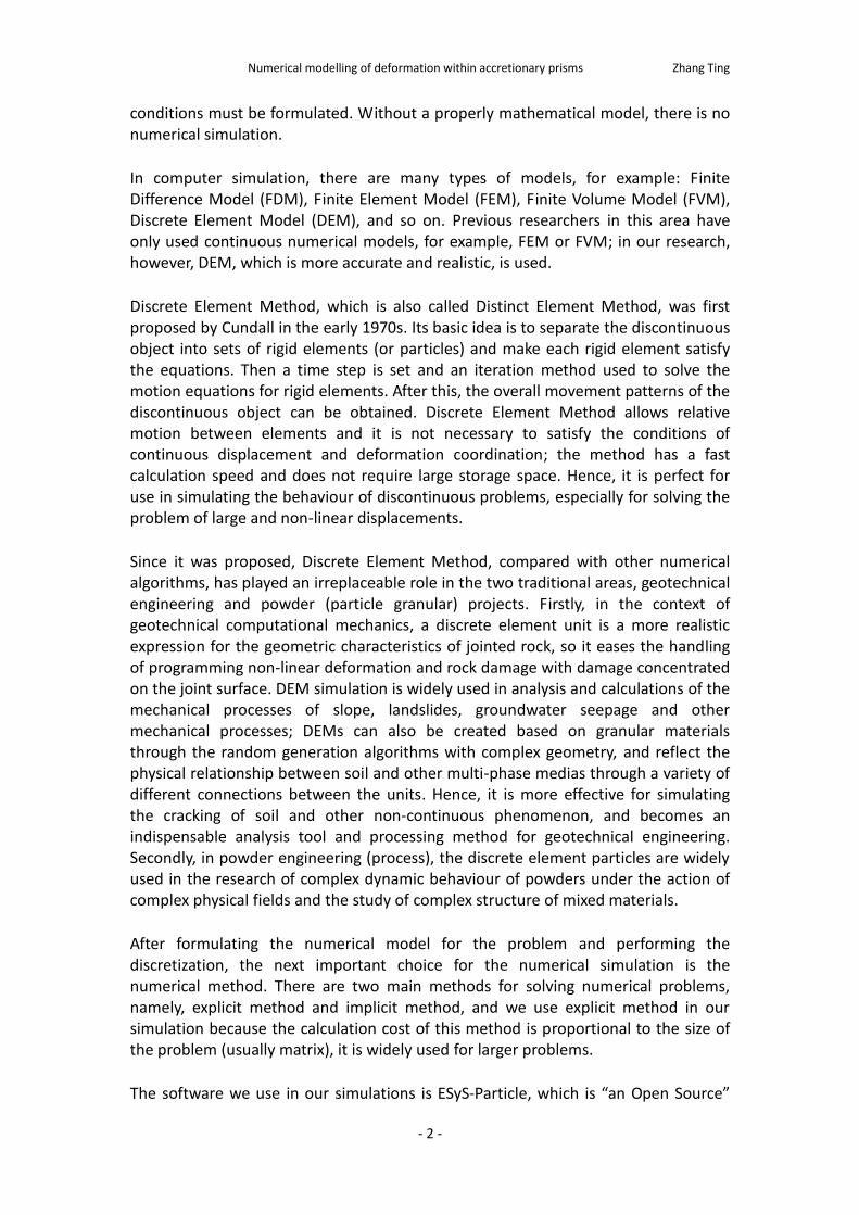
Like a physical model, a numerical model is set to be a 20m*1m box consisting of passively layered rocks. The model is shortened from one end (left wall or pushing wall) with a certain low velocity, 0.04mm/s, until 40 percentage of shortening is reached. The basement and the right wall are rigid and fixed. The friction coefficient of the basement is changed systematically between simulations to see the resulting behaviour of the model (Fig. 1).
Figure 1. The geometry of the model
2.2 Material Properties
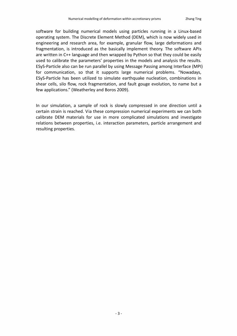
In order to simulate the behaviour of real rocks, we use real data from rocks in the upper crust. Here we list some of the mechanical properties for the models, most of which will stay constant during the whole simulation, although some will be changed to study their effect on the deformation.
Numerical modelling of deformation within accretionary prisms Zhang Ting
- 5 -
Table 1. Micro-properties of the model
Symbol Description Value
(kg/m3) Density of the rock 2600
cE (GPa) Young’s modulus of particles 50
max min/R R Ratio of maximum and minimum particle 2.5
c (MPa) Cohesion for the rock particles 45
c Particle contact friction coefficient 0.7
w Left wall friction coefficient 1.0
f Basement friction coefficient -
p Poisson rate 0.35
( ) Internal friction angle 0.4
g ( 2/m s ) Gravity 9.81
2.3 Model Lists
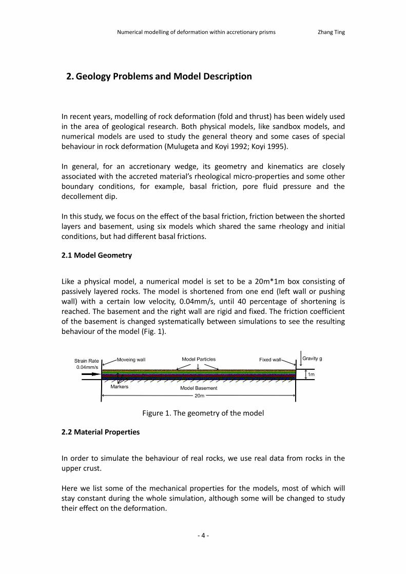
The series of six models are divided into four subsets: no- friction group, low-friction group, intermediate-friction group and high-friction group (Table 2).
Table 2. The friction coefficient of the models
Model Number The friction coefficient on the floor Mark
1 0.0 No-friction group
2 0.3 Low-friction group
3 0.5 Intermediate-friction group
4 0.7
5 0.9 High-friction group
6 1.0
NOTE: In the models’ design, some natural processes, for example, sedimentation, erosion and so on, are not included.
Numerical modelling of deformation within accretionary prisms Zhang Ting
- 6 -
3. Discrete Element Model
To solve the model we mentioned above, some numerical methods are needed to discrete the models. There are two mathematical approaches to calculating quantities which vary in space and time. One is the Eulerian numerical method, which is named after L. Euler, and the other is the Lagrangian numerical method. The Eulerian numerical method calculates quantities at points fixed in space, which means that the material is moving through the calculation points. Hence, it is usually used in Standard Finite Difference Method (FDM) or Finite Element Method (FEM). The Lagrangian numerical method, however, calculates quantities at points fixed to the material, that is, the calculation points are moving through space, and so it is usually used in Discrete Element Method (DEM) and Smooth Particle Hydrodynamics (SPH). Hence, in our model, the Lagrangian numerical method, specifically, Discrete Element Method (DEM) is used.
3.1 Introduction of Discrete Element Model
Numerical methods usually use discrete particles (or mesh) with limited degrees of freedom as a model to approximate object with infinite degrees of freedom. The discrete model has three elements: particles (or units), nodes and interactions. The shape of discrete element units can be many different types, but each of them has only one basic node (usually the centroid point of the unit). This unit is a physical element which is significantly different from the basic units formed by Finite Element Method, Boundary Element Method and other numerical methods (mesh element) because it has clear physical meaning. In addition, the interactions between nodes of the Discrete Element Method also have clear physical meaning, which is different from other numerical models. Therefore, we can define the discrete method simply as a numerical method, building a discrete model by using physically discrete units and interactions with clear physical meaning.
3.1.1 Discrete Elements
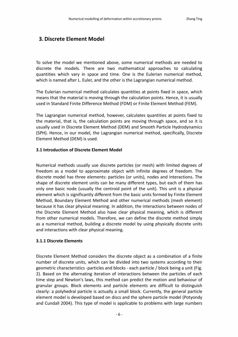
Discrete Element Method considers the discrete object as a combination of a finite number of discrete units, which can be divided into two systems according to their geometric characteristics -particles and blocks - each particle / block being a unit (Fig. 2). Based on the alternating iteration of interactions between the particles of each time step and Newton's laws, this method can predict the motion and behaviour of granular groups. Block elements and particle elements are difficult to distinguish clearly: a polyhedral particle is actually a small block. Currently, the general particle element model is developed based on discs and the sphere particle model (Potyondy and Cundall 2004). This type of model is applicable to problems with large numbers
Numerical modelling of deformation within accretionary prisms Zhang Ting
- 7 -
of particles and where the shape of units can be approximated by round, spherical or ellipsoidal particles. In this sense, the difference between block element and particle element is the contact model caused by the physical characteristics. In our simulation, we will use the particle element; this type of DEM is also called a Lattice Solid Model (Abe, Place et al. 2004).
Figure 2. The element of the numerical models: (a) Block element and (b) Particle element.
3.1.2 Interaction Model
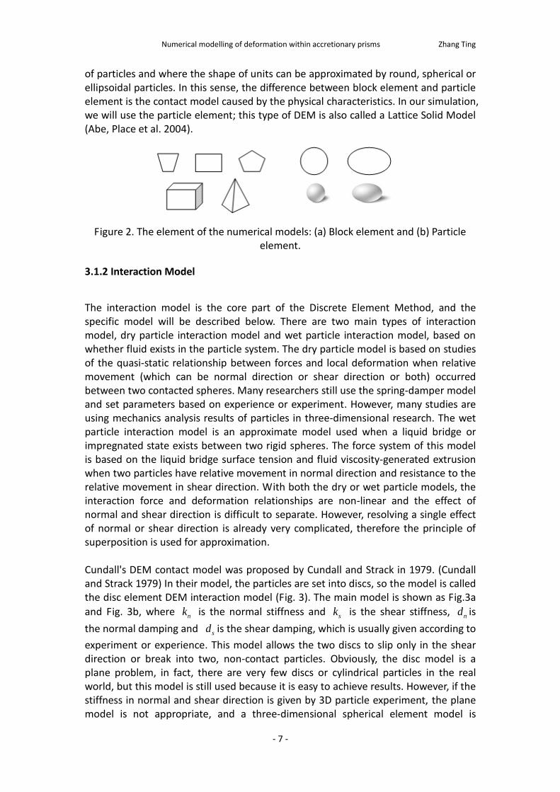
The interaction model is the core part of the Discrete Element Method, and the specific model will be described below. There are two main types of interaction model, dry particle interaction model and wet particle interaction model, based on whether fluid exists in the particle system. The dry particle model is based on studies of the quasi-static relationship between forces and local deformation when relative movement (which can be normal direction or shear direction or both) occurred between two contacted spheres. Many researchers still use the spring-damper model and set parameters based on experience or experiment. However, many studies are using mechanics analysis results of particles in three-dimensional research. The wet particle interaction model is an approximate model used when a liquid bridge or impregnated state exists between two rigid spheres. The force system of this model is based on the liquid bridge surface tension and fluid viscosity-generated extrusion when two particles have relative movement in normal direction and resistance to the relative movement in shear direction. With both the dry or wet particle models, the interaction force and deformation relationships are non-linear and the effect of normal and shear direction is difficult to separate. However, resolving a single effect of normal or shear direction is already very complicated, therefore the principle of superposition is used for approximation. Cundall's DEM contact model was proposed by Cundall and Strack in 1979. (Cundall and Strack 1979) In their model, the particles are set into discs, so the model is called the disc element DEM interaction model (Fig. 3). The main model is shown as Fig.3a
and Fig. 3b, where nk is the normal stiffness and sk is the shear stiffness, nd is
the normal damping and sd is the shear damping, which is usually given according to
experiment or experience. This model allows the two discs to slip only in the shear direction or break into two, non-contact particles. Obviously, the disc model is a plane problem, in fact, there are very few discs or cylindrical particles in the real world, but this model is still used because it is easy to achieve results. However, if the stiffness in normal and shear direction is given by 3D particle experiment, the plane model is not appropriate, and a three-dimensional spherical element model is
Numerical modelling of deformation within accretionary prisms Zhang Ting
- 8 -
needed (Mindlin and Deresiewicz 1953; Johnson 1985).
Figure 3. Interaction models: (a) normal effect; (b) shear effect; (c) rotating effect; Cundall’s DEM model (a+b); Mara and Place’s DEM model (a+b+c).
The model we use, the Lattice Solid Model, is of this type and was described by Mora and Place in 1994 and 1999 (Mora and Place 1994; Place and Mora 1999). This model considers normal, shear and also rotational effect between two particles. The interactions (friction, elastic force and so on) are simulated between two near particles based on their radius, mass, position and velocity. These interactions will be described later.
3.2 Model Theory and Equations
The dynamics of particles are governed by Newton’s laws. In the DEM models, the calculation preformation contains the force theory for spherical particles and time discretization (Law of motion). As we discussed above, the interactions between two balls or a ball and a wall are formed and broken during the simulation process automatically. (Johnson 1985; Poschel and Schwager 2005) At the beginning of the simulation, the particle and wall positions and contact set are initialized. After that, the simulation process can be described as the repeating of the follow two steps: 1. Calculate contact force and relative motion of the interactions between each two the space discretization objects (particles and walls); 2. Calculate the resultant force and moment based on the contact forces and boundary condition, and then update the position and velocity for each particle and wall. For 2D models like our model, the model can be simplified by apply the model in the
first and second direction ( 1x and 2x ) and only apply moments ( 3M ) & rotational
velocity ( 3 ) in the third direction.
Numerical modelling of deformation within accretionary prisms Zhang Ting
- 9 -
3.2.1 Force Theory for Spherical Particles
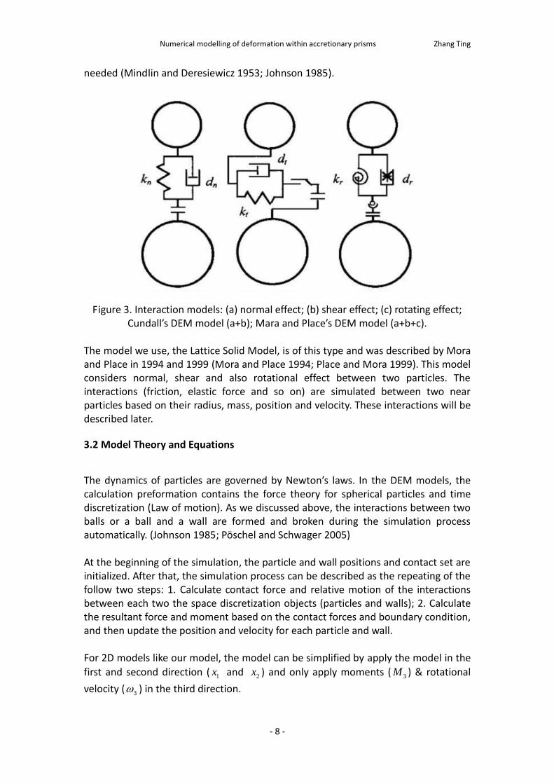
As we discussed, in DEM models, the model are dispersed into small particles. The contact force and relative displacement between two particles could be calculated based on the distance between them. If we draw a line between two contact particles, the contact force between them could be decomposed into a normal force which acting along the line and a shear force perpendicular to the line. (Fig. 4) The distance between the ball centres:
[2] [1] [2] [1] [2] [1]
i i i i i id x x x x x x (3.1)
where [1]
ix and [2]
ix are the vectors showing the position of the centres of ball 1
and 2. The overlap , is defined by the relative displacement along the normal direction, given by:
1 2R R d (3.2)
where 1R and 2R are the radius of ball 1
and 2, respectively.
As we said above, the contact force iF can
be decomposed into a normal force and a shear force:
n s
i i iF F F (3.3)
where n
iF and s
iF means the normal and
shear force vectors. The normal force could be calculated by:
n nF k (3.4)
where nk is the normal stiffness at the contact. The shear force is calculated based on the relative shear motion (or shear velocity)
sV , which is given by:
Figure 4. Spherical Element Models: α is the pseudo overlap area, d is the
distance between two particles and a is the contact radius.
Numerical modelling of deformation within accretionary prisms Zhang Ting
- 10 -
[2] [1] [2] [ ] [2] [1] [ ] [1]
3 3
s C C
i i i k k k kV x x t x x x x (3.5)
where [ ]j
ix and [ ]
3
j are the translational and rotational velocity, respectively, and [ ]C
ix is the location of the contact point, given by:
[2] [1]
[ ] [1]
1
1
2
C i ii i
x xx x R
d
(3.6)
and [1] [2] [2] [1]
2 2 1 1,i
x x x xt
d d
Hence, the displacement increment in shear direction over a time step t is given by:
s sU V t (3.7) The shear force increment is:
s s sF k U (3.8)
where sk is the shear stiffness at the contact. The shear force is the summary of the old shear force:
s s s nF F F F (3.9)
where is the friction coefficient.
After these calculations, the final contact force and moment of the two balls are:
[1] [1]
[2] [2]
[1] [ ] [1] [1]
3 3
[2] [ ] [2] [2]
3 3
n s
i i i
i i i
i i i
C
i i k
C
i i k
F F n F t
F F F
F F F
M e x x F M
M e x x F M
(3.10)
where [ ]j
iF and [ ]
3
jM are the force and moment for particle j .
3.2.2 Time Discretization: Law of motion
In the time discretization, the centred finite difference method with a time step t
Numerical modelling of deformation within accretionary prisms Zhang Ting
- 11 -
is used. There are two essential formulas, one calculate translational motion from force and the other one calculate rotational motion from moment. The translational motion formula is described as:
i i iF m x g (Translational motion) (3.11)
where iF is the resultant force, the sum of applied forces acting on the particle; m
is the total mass of the particle; and ig is the body force acceleration vector (e.g.,
gravity). The rotational motion can be described as:
i iM H (3.12)
where iH is the angular momentum of the particle, and iM is the resultant
moment acting on the particle. Since we are using a 2D model, the particles are treated as disk, the angular
accelerations 1 2 0 . Thus, the Euler’s equation of motion is given by:
2
3 3 3 32
mRM I
(Rotational motion) (3.13)
where 3I and 3 are the moment and angular accelerations in the third direction.
To solve the equations of motion by the centred finite difference, at the mid-intervals
of / 2t nt , the quantities ix and 3 are calculated, and at the intervals of
t nt , the quantities ix , ix , i , iF and 3M are calculated.
The translational and rotational accelerations at time t are calculated by the following formulas:
( ) ( /2) ( /2)
( ) ( /2) ( /2)
3 3 3
1
1
t t t t t
i i i
t t t t t
x x xt
t
(3.14)
Insert these formulas into Eqs. (3.11) and (3.13), the translational and rotational velocities at time / 2t t are:
( /2) ( /2)
( /2) ( /2) 33
t
t t t t ii i i
t
t t t t
i
Fx x g t
m
Mt
I
(3.15)
Numerical modelling of deformation within accretionary prisms Zhang Ting
- 12 -
Finally, the positions of the particles are described as
( /2)t t t t t
i i ix x x t (3.16)
To sum up, the law of motion is: 1. Calculate ( /2)t t
ix and ( /2)
3
t t from the values
of ( /2)t t
ix , ( /2)
3
t t , tix , t
iF and 3
tM ; 2. Then, calculate t t
ix from Eq.
(3.16). The values of t t
iF and
3
t tM
used for the next cycle are obtained by the
force theory part.
3.3 DEM Model Details
The model region can be represented in two dimensions (Fig. 6). All of the three walls, left wall, right wall and floor, are rigid boundaries. The left wall is moving to the right, shortening the layered stratigraphy at a particular slow speed under the influence of gravity. The objective is to simulate the deformation in the layered lithology and find the relationship between the final behaviour of the layer and the parameters we chose. The procedure for solving the problem is:
1. Define material properties, initial and boundary conditions.
2. Solve the problem using numerical method.
3. Systematically change the parameter we are interested in and re-run the model.
4. Study the solution using post-processing techniques.
We create the geometry and export the data to the software. The boundary conditions and rock properties are set through parameterized case files. Esys-Particle will calculate the results and record the data until a specified time is reached.
3.3.1 Particle Packing Algorithm
After setting the geometry of the model, the next step is to fill the model with a dense packing of random spherical particles, that is, the particles are of random size in particular region.
There are two methods to fill random particles, namely, constructive method (also particle insertion method) and dynamic method (Schopfer, Abe et al. 2009). In our simulation, the former will be used.
The dynamic method first generates a lot of particles radii in a certain range to fill the model domain and then allow them move without friction for adjustment. If the isotropic stress is too large, the radii of the particles will be modified by multiply a
Numerical modelling of deformation within accretionary prisms Zhang Ting
- 13 -
number around 1 to reduce it. This process will continue repeating until all the particles have at least 3 contacts points and the mean of the normal force among them is lower than a given value (Schopfer, Abe et al. 2009).
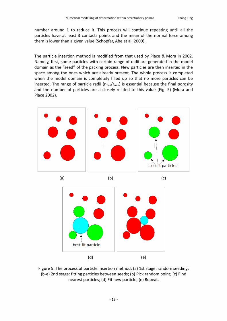
The particle insertion method is modified from that used by Place & Mora in 2002. Namely, first, some particles with certain range of radii are generated in the model domain as the “seed” of the packing process. New particles are then inserted in the space among the ones which are already present. The whole process is completed when the model domain is completely filled up so that no more particles can be inserted. The range of particle radii (rmax/rmin) is essential because the final porosity and the number of particles are a closely related to this value (Fig. 5) (Mora and Place 2002).
(a) (b) (c)
(d) (e)
Figure 5. The process of particle insertion method: (a) 1st stage: random seeding; (b-e) 2nd stage: fitting particles between seeds; (b) Pick random point; (c) Find
nearest particles; (d) Fit new particle; (e) Repeat.
Numerical modelling of deformation within accretionary prisms Zhang Ting
- 14 -
This method results in particle packing with the following features:
● Closely packed
● Fully connected
● Each particle has at least 3 neighbours
● No initial stress/force exists between the particles
● Particle range size can be prescribed
● Power law particle size distribution is generated
3.3.2 Force Models
There is no doubt that all the movements in the model are due to the applied by the moving left wall. And as we have mentioned above, the whole numerical model is based on the interaction model system. In this system, the force can be divided into the following types: 1. The interaction of a particle with its nearest neighbours, i.e. the particles it
touches. For example, free elastic force, bonded elastic force and friction force.
2. The interaction of this particle with other objects, such as walls and mesh objects acting as boundary conditions.
3. Global force fields (i.e. gravity).
4. A velocity dependent damping.
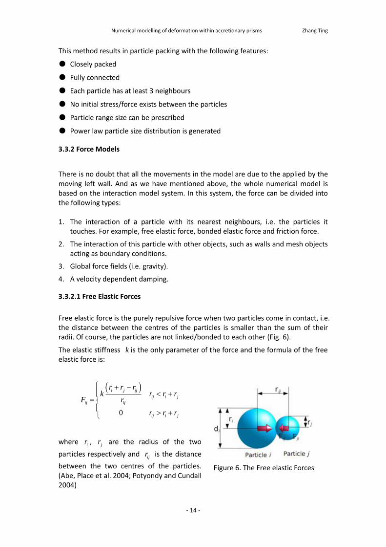
3.3.2.1 Free Elastic Forces
Free elastic force is the purely repulsive force when two particles come in contact, i.e. the distance between the centres of the particles is smaller than the sum of their radii. Of course, the particles are not linked/bonded to each other (Fig. 6).
The elastic stiffness k is the only parameter of the force and the formula of the free elastic force is:
0
i j ij
ij i j
ij ij
ij i j
r r rk r r r
F r
r r r
where ir , jr are the radius of the two
particles respectively and ijr is the distance
between the two centres of the particles. (Abe, Place et al. 2004; Potyondy and Cundall 2004)
Figure 6. The Free elastic Forces
Numerical modelling of deformation within accretionary prisms Zhang Ting
- 15 -
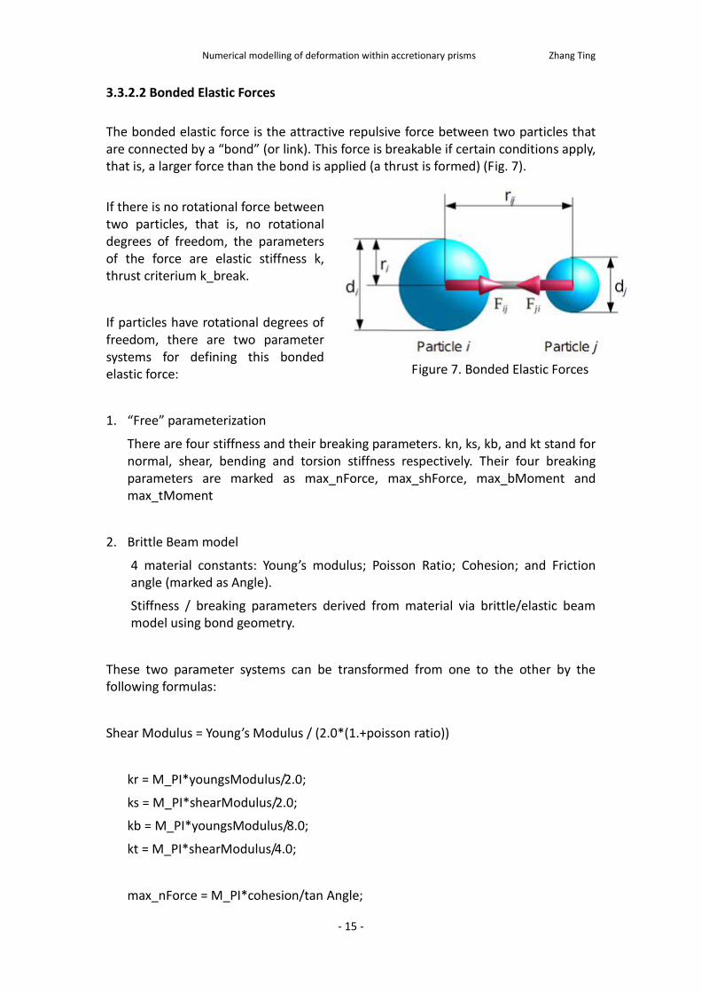
3.3.2.2 Bonded Elastic Forces
The bonded elastic force is the attractive repulsive force between two particles that are connected by a “bond” (or link). This force is breakable if certain conditions apply, that is, a larger force than the bond is applied (a thrust is formed) (Fig. 7).
If there is no rotational force between two particles, that is, no rotational degrees of freedom, the parameters of the force are elastic stiffness k, thrust criterium k_break.
If particles have rotational degrees of freedom, there are two parameter systems for defining this bonded elastic force:
1. “Free” parameterization
There are four stiffness and their breaking parameters. kn, ks, kb, and kt stand for normal, shear, bending and torsion stiffness respectively. Their four breaking parameters are marked as max_nForce, max_shForce, max_bMoment and max_tMoment
2. Brittle Beam model
4 material constants: Young’s modulus; Poisson Ratio; Cohesion; and Friction angle (marked as Angle).
Stiffness / breaking parameters derived from material via brittle/elastic beam model using bond geometry.
These two parameter systems can be transformed from one to the other by the following formulas:
Shear Modulus = Young’s Modulus / (2.0*(1.+poisson ratio))
kr = M_PI*youngsModulus/2.0;
ks = M_PI*shearModulus/2.0;
kb = M_PI*youngsModulus/8.0;
kt = M_PI*shearModulus/4.0;
max_nForce = M_PI*cohesion/tan Angle;
Figure 7. Bonded Elastic Forces
Numerical modelling of deformation within accretionary prisms Zhang Ting
- 16 -
max_shForce = M_PI*cohesion;
max_bMoment = M_PI*cohesion/tan Angle/4.0;
max_tMoment = M_PI*cohesion/2.0;
Where M_PI stands for = 3.14159265358979323846.
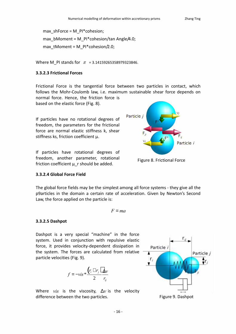
3.3.2.3 Frictional Forces
Frictional Force is the tangential force between two particles in contact, which follows the Mohr-Coulomb law, i.e. maximum sustainable shear force depends on normal force. Hence, the friction force is based on the elastic force (Fig. 8).
If particles have no rotational degrees of freedom, the parameters for the frictional force are normal elastic stiffness k, shear stiffness ks, friction coefficient μ.
If particles have rotational degrees of freedom, another parameter, rotational friction coefficient μ_r should be added.
3.3.2.4 Global Force Field
The global force fields may be the simplest among all force systems - they give all the p9articles in the domain a certain rate of acceleration. Given by Newton’s Second Law, the force applied on the particle is:
F ma=
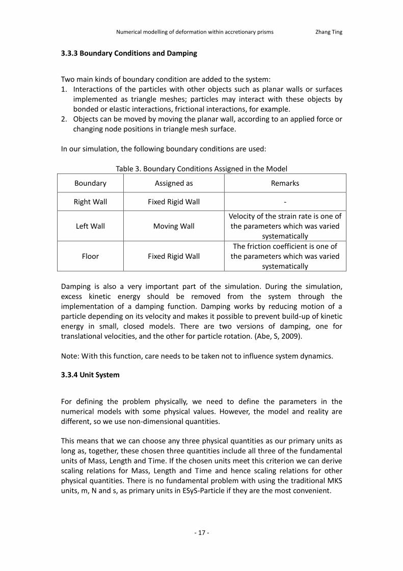
3.3.2.5 Dashpot
Dashpot is a very special “machine” in the force system. Used in conjunction with repulsive elastic force, it provides velocity-dependent dissipation in the system. The forces are calculated from relative particle velocities (Fig. 9).
( )*
2
i j
ij
r r vf vis
r
+ D= -
Where vis is the viscosity, vD is the velocity difference between the two particles.
Figure 8. Frictional Force
Figure 9. Dashpot
Numerical modelling of deformation within accretionary prisms Zhang Ting
- 17 -
3.3.3 Boundary Conditions and Damping
Two main kinds of boundary condition are added to the system: 1. Interactions of the particles with other objects such as planar walls or surfaces
implemented as triangle meshes; particles may interact with these objects by bonded or elastic interactions, frictional interactions, for example.
2. Objects can be moved by moving the planar wall, according to an applied force or changing node positions in triangle mesh surface.
In our simulation, the following boundary conditions are used:
Table 3. Boundary Conditions Assigned in the Model
Boundary Assigned as Remarks
Right Wall Fixed Rigid Wall -
Left Wall Moving Wall Velocity of the strain rate is one of the parameters which was varied
systematically
Floor Fixed Rigid Wall The friction coefficient is one of
the parameters which was varied systematically
Damping is also a very important part of the simulation. During the simulation, excess kinetic energy should be removed from the system through the implementation of a damping function. Damping works by reducing motion of a particle depending on its velocity and makes it possible to prevent build-up of kinetic energy in small, closed models. There are two versions of damping, one for translational velocities, and the other for particle rotation. (Abe, S, 2009). Note: With this function, care needs to be taken not to influence system dynamics.
3.3.4 Unit System
For defining the problem physically, we need to define the parameters in the numerical models with some physical values. However, the model and reality are different, so we use non-dimensional quantities.
This means that we can choose any three physical quantities as our primary units as long as, together, these chosen three quantities include all three of the fundamental units of Mass, Length and Time. If the chosen units meet this criterion we can derive scaling relations for Mass, Length and Time and hence scaling relations for other physical quantities. There is no fundamental problem with using the traditional MKS units, m, N and s, as primary units in ESyS-Particle if they are the most convenient.
Numerical modelling of deformation within accretionary prisms Zhang Ting
- 18 -
In many cases, however, using MKS units is not as convenient as using another set of primary units. The software can sometimes hard to achieve a good packing of particles if the mean radius is significantly different from 1.0 (i.e. if particles have radii of ~10000.0 unit, the results may not be accurate). It is always best to check the particle packing before starting a simulation e.g. by visualizing the particles in preview. Hence, it is better to change the primary units relate to a potential problem with generating particle geometries. If the particle packing is not adequate due to very large particle radii, we may need to choose a different set of primary units so that particles have a mean radius of ~ 1.
For comparison of simulations with laboratory experiments, I have found that using m, sec and grams is very helpful in our project. These units mean that forces will be reported in Newton, and velocities will be reported in m/s. Since it is often the case that we wish to compare forces or velocities measured in the real world with those in simulations, this choice of units is quite convenient.
If we use meters for length units, choosing kilo-Newton for force units is suitable:
a) We can calibrate model parameters so that the peak force reported by a UCS simulation is exactly the same numerical value as the force measured in the equivalent lab experiment.
b) When we measure length in mm and force in kN, stresses are reported by simulations in GPa (which is convenient when we want to measure quantities like Young's modulus and peak stress!).
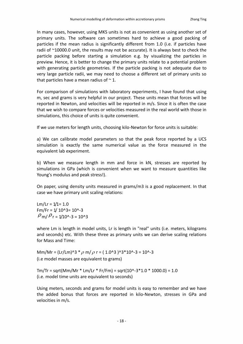
On paper, using density units measured in grams/m3 is a good replacement. In that case we have primary unit scaling relations:
Lm/Lr = 1/1= 1.0 Fm/Fr = 1/ 10^3= 10^-3 r m/ r r = 1/10^-3 = 10^3
where Lm is length in model units, Lr is length in "real" units (i.e. meters, kilograms and seconds) etc. With these three as primary units we can derive scaling relations for Mass and Time:
Mm/Mr = (Lr/Lm)^3 * m/ r = ( 1.0^3 )^3*10^-3 = 10^-3
(i.e model masses are equivalent to grams)
Tm/Tr = sqrt(Mm/Mr * Lm/Lr * Fr/Fm) = sqrt(10^-3*1.0 * 1000.0) = 1.0 (i.e. model time units are equivalent to seconds)
Using meters, seconds and grams for model units is easy to remember and we have the added bonus that forces are reported in kilo-Newton, stresses in GPa and velocities in m/s.
Numerical modelling of deformation within accretionary prisms Zhang Ting
- 19 -
3.3.5 Rotational and Non-Rotational Particles
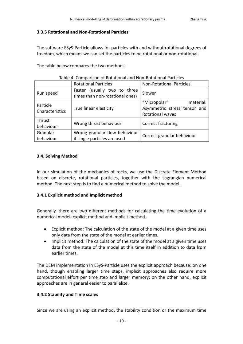
The software ESyS-Particle allows for particles with and without rotational degrees of freedom, which means we can set the particles to be rotational or non-rotational. The table below compares the two methods:
Table 4. Comparison of Rotational and Non-Rotational Particles
Rotational Particles Non-Rotational Particles
Run speed Faster (usually two to three times than non-rotational ones)
Slower
Particle Characteristics
True linear elasticity “Micropolar” material: Asymmetric stress tensor and Rotational waves
Thrust behaviour
Wrong thrust behaviour Correct fracturing
Granular behaviour
Wrong granular flow behaviour if single particles are used
Correct granular behaviour
3.4. Solving Method
In our simulation of the mechanics of rocks, we use the Discrete Element Method based on discrete, rotational particles, together with the Lagrangian numerical method. The next step is to find a numerical method to solve the model.
3.4.1 Explicit method and Implicit method
Generally, there are two different methods for calculating the time evolution of a numerical model: explicit method and implicit method.
Explicit method: The calculation of the state of the model at a given time uses only data from the state of the model at earlier times.
Implicit method: The calculation of the state of the model at a given time uses data from the state of the model at this time itself in addition to data from earlier times.
The DEM implementation in ESyS-Particle uses the explicit approach because: on one hand, though enabling larger time steps, implicit approaches also require more computational effort per time step and larger memory; on the other hand, explicit approaches are in general easier to parallelize.
3.4.2 Stability and Time scales
Since we are using an explicit method, the stability condition or the maximum time
Numerical modelling of deformation within accretionary prisms Zhang Ting
- 20 -
step to be used in our simulation should be considered. In our model, time step size is limited by the time it takes to transmit information (force and so on) across the smallest particle. Here, the speed of transmitting information should be carefully considered, especially in the case of models with rotational particles and free bond stiffness parameterization due to “rotational” waves. We can easily find that the transmitting speed has the following characteristics:
– Determined by stiffness and particle mass
– Can be calculated directly for regular particle packing (proportional sqrt(k/m) )
– Close to theoretical value for random packing
– Can be measured It follows from the discussion above that the time step is always limited by the smallest particles in the model.
To get a stable time step in the simulation, we should look at what time scales are present in the model. The length scale can be selected as the radius r of the particles, as this is the most important length involved in the problem. The mass scale can be taken as the particle mass m (if particles have different radii and masses, the largest, smallest or average can be chosen; however, the smallest is the most functional one, so we use that). Actually, in the simulation, there are many time scales in the model, for example:
We use gravity in the model, so there is a time scale 1 min2* /T r g ; we also have
spring constant K in the model , so that we have another time scale for the max
K that 2 min max/T m K ; in addition, There is also a compression velocity /v l t ,
so that 3 min2* /T r v , etc.
To prevent these instabilities, our time step shall be significantly less than any time
scale of the problem, e.g. 0.1min idt T .
However, in most of the problems, the min iT is min max/m K , which is the case in
our model, which is why I mention the time step as above.
If a larger time step is used, the whole model will be unstable, may produce some unrealistic results or may even cause the process diverging. Then we face the problem of how to have a larger time step and also produce a stable system - this is called a “time scale problem”. Time scale problem is common, and many systems which are interesting to model contain widely differing time scales; for example in earthquake dynamics: rupture time (sec) vs. inter-event time (year – centuries) and thrust: breaking time vs. loading time. The problem is that time step size is determined by the shortest time scale in the model, and total simulated time is determined by the longest time scale.
Numerical modelling of deformation within accretionary prisms Zhang Ting
- 21 -
The shortest time scale in the model is generally the time it takes to transmit information across the smallest particle, i.e. P-wave speed divided by particle diameter. The number of time steps is simulated time divided by time step size, that is, a wide range of time scales results in a large number of time steps To solve this time scale problem, the following suggestions are helpful: 1. Shorten the longest time scale by increasing the loading speed
– Potential issues with changing system dynamics, i.e. Quasi-static vs. Dynamic
– Need to keep time scales separated 2. Lengthen the time step by reducing the P-Wave speed, for example by reducing
the elastic stiffness of increasing the particle density (weight)
– Need to keep time scales separated – problems if loading speeds get too close to breaking speeds
3. Always try different amounts of “fixing” to see whether system dynamics are changed! (Abe 2009)

Numerical modelling of deformation within accretionary prisms Zhang Ting
- 22 -
4. Implementation and Post-processing
4.1 Algorithm
The programming algorithm (Pseudo code) can be written as follows: A. Setting parameters for implementation
a) Time step, number of iteration, and so on B. Initialization:
a) Initialize the ESyS-Particle simulation object: i. Number of worker processes
ii. How to partition the space iii. Initialize the neighbour search and specify the type of particles iv. Grid spacing v. Cut off distance for neighbour list
b) Set the time step increment for the simulation: C. Create a block of random particles:
a) Maximum and minimum radius of particles b) Size of the box c) Particle tag
D. Create rotational elastic-brittle bonds between particles a) Stress stiffness and break force (normal, shear, bending and torsion)
E. Create walls of the model a) Left wall, right wall and floor
F. Create friction interaction between unbounded particles a) Coefficient of dynamic/static friction
G. Create friction on the walls (if needed) a) Coefficient of friction on the left wall/floor
H. Create exclusion between bonded and friction interaction I. Create particle elastic repulsion from the walls
a) Left wall, right wall and floor J. Specify the direction and magnitude of gravity
a) Acceleration of gravity K. Add damping to the system
a) Translational damping and rotational damping L. Add a wall loader to move the left wall
a) Velocity of the strain M. Add the results saver N. Add POVsnop camera (a software to take pictures of the particles) O. Perform simulation
Numerical modelling of deformation within accretionary prisms Zhang Ting
- 23 -
4.2 Parallel Implementation
The traditional computer simulation methods, which are limited by the hardware technique, are not suitable for tackling the problems we study nowadays. Hence, people divide the problem into several parts and solve them on many computers and then assemble the results. This technique, parallel computing, has been improved and become an essential way of solving the problems. The following table shows the features of serial computation and parallel computing:
Table 5. The features of serial computation and parallel computing
serial computation parallel computing
Run on a single computer having a single CPU.
A problem is broken into a discrete series of instructions.
Instructions are executed one after another.
Only one instruction may be executed at any moment in time.
The simultaneous use of multiple computing resources to solve a computational problem.
A problem is broken into discrete parts that can be solved concurrently.
Each part is further broken down to a series of instructions.
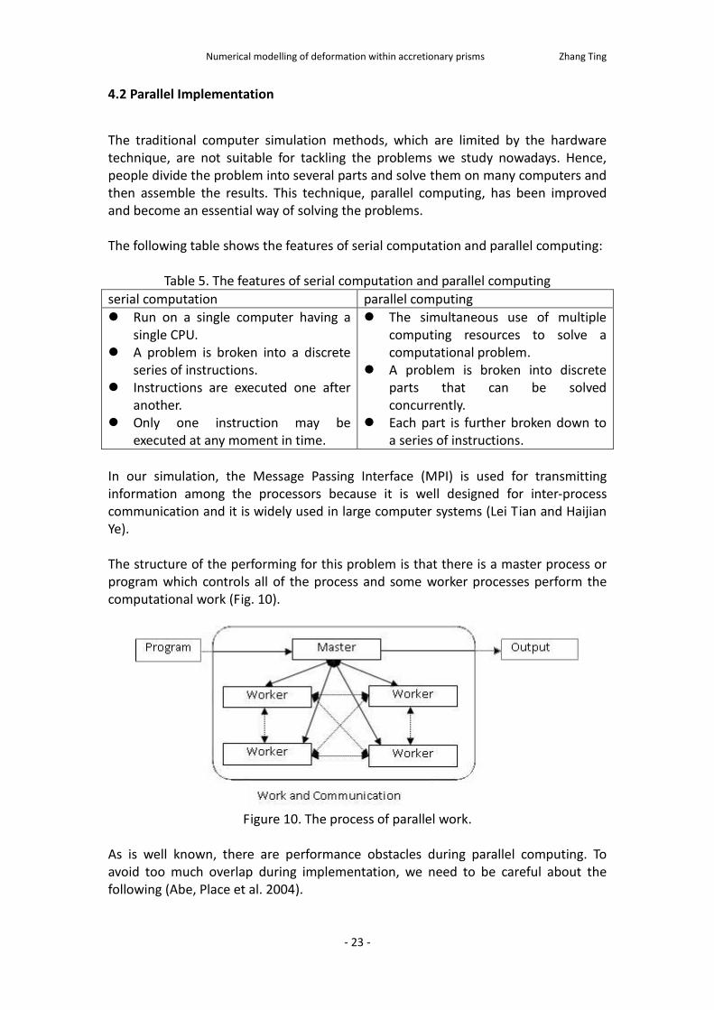
In our simulation, the Message Passing Interface (MPI) is used for transmitting information among the processors because it is well designed for inter-process communication and it is widely used in large computer systems (Lei Tian and Haijian Ye). The structure of the performing for this problem is that there is a master process or program which controls all of the process and some worker processes perform the computational work (Fig. 10).
Figure 10. The process of parallel work.
As is well known, there are performance obstacles during parallel computing. To avoid too much overlap during implementation, we need to be careful about the following (Abe, Place et al. 2004).
Numerical modelling of deformation within accretionary prisms Zhang Ting
- 24 -
1. Communication: Use asynchronous communication and message probing; 2. Load balance: Choose pivot carefully, use different strategies; 3. Synchronization: Split communicator (topology) in each step to avoid global
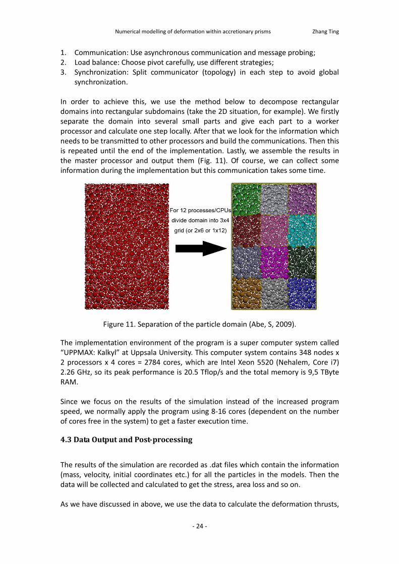
synchronization. In order to achieve this, we use the method below to decompose rectangular domains into rectangular subdomains (take the 2D situation, for example). We firstly separate the domain into several small parts and give each part to a worker processor and calculate one step locally. After that we look for the information which needs to be transmitted to other processors and build the communications. Then this is repeated until the end of the implementation. Lastly, we assemble the results in the master processor and output them (Fig. 11). Of course, we can collect some information during the implementation but this communication takes some time.
Figure 11. Separation of the particle domain (Abe, S, 2009).
The implementation environment of the program is a super computer system called “UPPMAX: Kalkyl” at Uppsala University. This computer system contains 348 nodes x 2 processors x 4 cores = 2784 cores, which are Intel Xeon 5520 (Nehalem, Core i7) 2.26 GHz, so its peak performance is 20.5 Tflop/s and the total memory is 9,5 TByte RAM. Since we focus on the results of the simulation instead of the increased program speed, we normally apply the program using 8-16 cores (dependent on the number of cores free in the system) to get a faster execution time.
4.3 Data Output and Post-processing
The results of the simulation are recorded as .dat files which contain the information (mass, velocity, initial coordinates etc.) for all the particles in the models. Then the data will be collected and calculated to get the stress, area loss and so on. As we have discussed in above, we use the data to calculate the deformation thrusts,
Numerical modelling of deformation within accretionary prisms Zhang Ting
- 25 -
area loss of the models, wedge height versus length, force on the left wall and basement, displacement of the particles, movement trends and internal stress of the models. Here, we use an open software called “Paraview” to do the data mining and some figure visualization. In addition, we use Matlab to produce some figures during post- processing.
Numerical modelling of deformation within accretionary prisms Zhang Ting
- 26 -
5. Results
In this section, the simulation results are presented to explain the effect of basal friction on model deformation. Six main models are discussed here to show the effect of the friction on basement. The first model is a no-friction one; the second model is a low-friction one; the next two are intermediate-friction ones; and the last two are high-friction ones.
During the process of shortening, some structure (usually a wedge) formed in the model including many folds and thrusts. Koyi and some other researchers (Koyi 1991; Koyi 1995; Storti and Mcclay 1995; Storti, Salvini et al. 1997) believe that at the early age of the shortening process, conjugate kink folds which are closely spaced will form, and then thrust will form because of the forelimbs are narrowed by the further shortening. After that, with the continuous shortening, the wedge will become higher and longer since new thrusts will accrete in the foot of it. This evolution is similar to many previous models of an accretionary wedge.
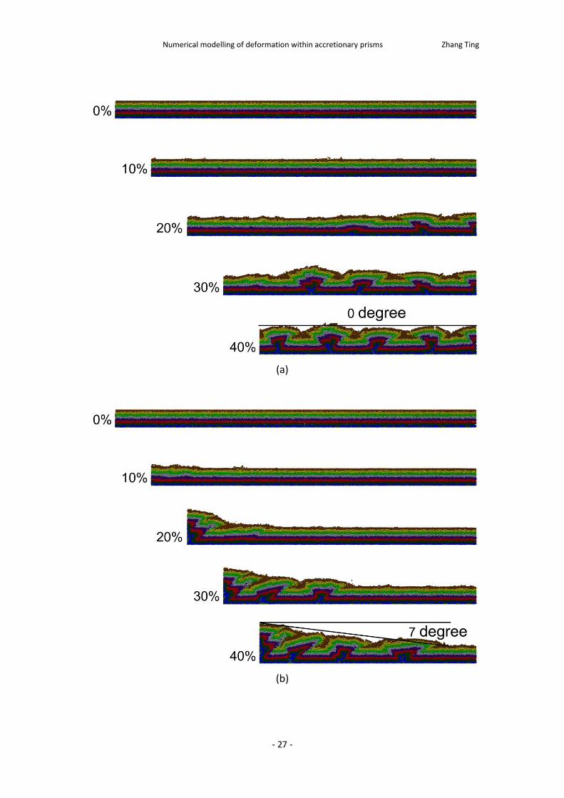
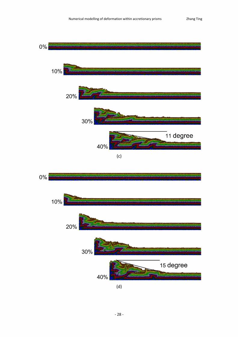
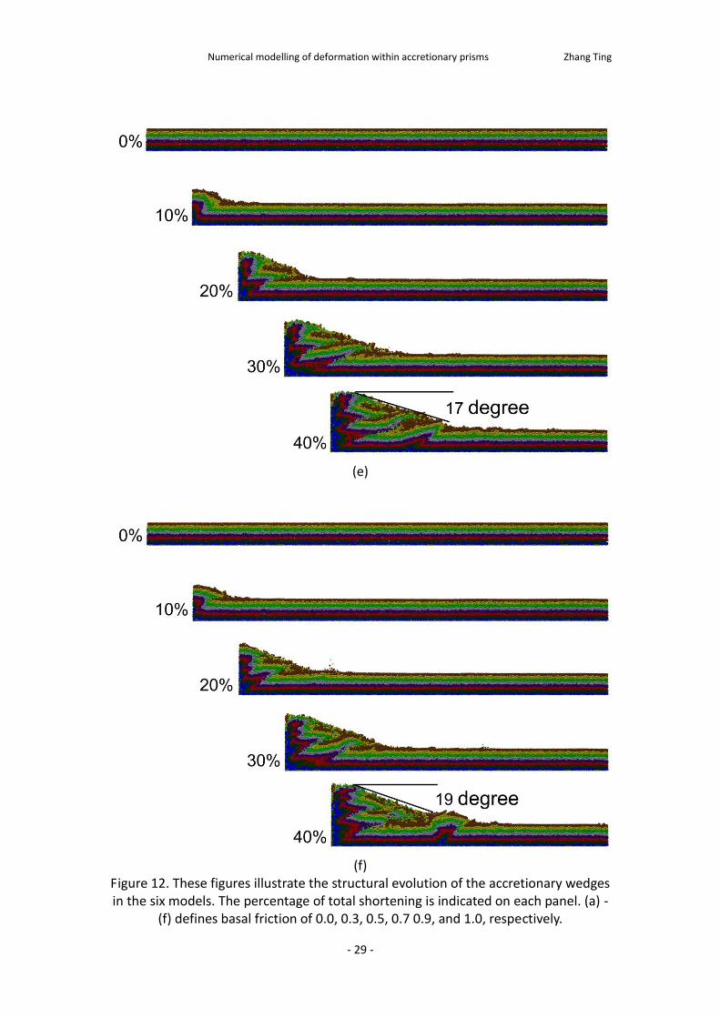
5.1 Evolution of models
The models are shortened from the left side with a certain low velocity, 0.04mm/s, until 40% bulk shortening is reached. During the shortening, the particles near the left hand boundary created a deformed accretionary wedge, except in the no friction model (Fig. 12).
In the 0.0f model, the thrust forms first in the right hard part of the model
because of the friction coefficient on the left and right wall are 0wl and
0wr . Then, the deformed area increases very fast until the whole domain is
deformed, in which all of the fractures distribute evenly and symmetrically (Fig. 12a).
In the other models, 0.1,9.0,7.0,5.0,3.0f , certain features are common. The
process could be divided into two stages. In the early stage, the wedge deforms internally as a complementary process because of transmitting of the compressing force overcome the basal friction, and quickly grows in order to reach a critical wedge taper. (Koyi 1995) In the later stage, the wedge increases both in length and height under the pushing force but the slope angle almost stays the same (Fig. 12b-12f).
Numerical modelling of deformation within accretionary prisms Zhang Ting
- 27 -
(a)
(b)
Numerical modelling of deformation within accretionary prisms Zhang Ting
- 28 -
(c)
(d)
Numerical modelling of deformation within accretionary prisms Zhang Ting
- 29 -
(e)
(f)
Figure 12. These figures illustrate the structural evolution of the accretionary wedges in the six models. The percentage of total shortening is indicated on each panel. (a) -
(f) defines basal friction of 0.0, 0.3, 0.5, 0.7 0.9, and 1.0, respectively.
Numerical modelling of deformation within accretionary prisms Zhang Ting
- 30 -
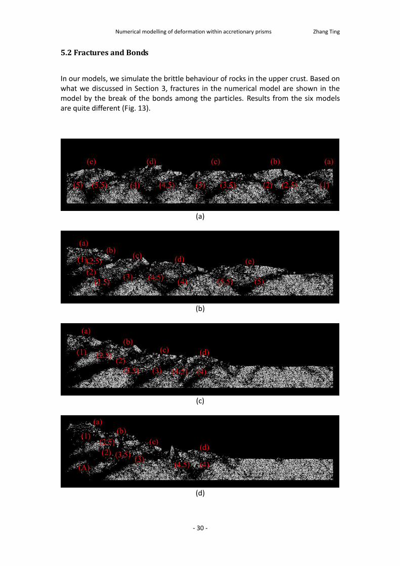
5.2 Fractures and Bonds
In our models, we simulate the brittle behaviour of rocks in the upper crust. Based on what we discussed in Section 3, fractures in the numerical model are shown in the model by the break of the bonds among the particles. Results from the six models are quite different (Fig. 13).
(a)
(b)
(c)
(d)
Numerical modelling of deformation within accretionary prisms Zhang Ting
- 31 -
(e)
(f)
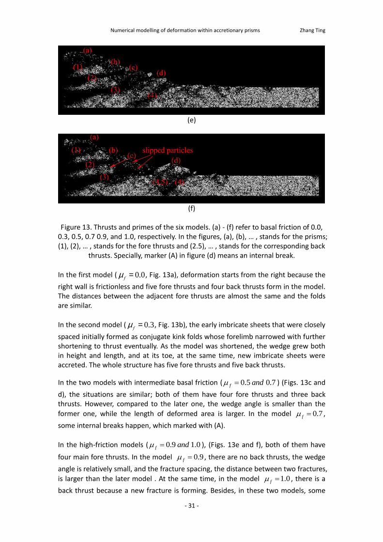
Figure 13. Thrusts and primes of the six models. (a) - (f) refer to basal friction of 0.0,
0.3, 0.5, 0.7 0.9, and 1.0, respectively. In the figures, (a), (b), … , stands for the prisms; (1), (2), … , stands for the fore thrusts and (2.5), … , stands for the corresponding back
thrusts. Specially, marker (A) in figure (d) means an internal break.
In the first model ( 0.0f
m = , Fig. 13a), deformation starts from the right because the
right wall is frictionless and five fore thrusts and four back thrusts form in the model. The distances between the adjacent fore thrusts are almost the same and the folds are similar.
In the second model ( 0.3f
m = , Fig. 13b), the early imbricate sheets that were closely
spaced initially formed as conjugate kink folds whose forelimb narrowed with further shortening to thrust eventually. As the model was shortened, the wedge grew both in height and length, and at its toe, at the same time, new imbricate sheets were accreted. The whole structure has five fore thrusts and five back thrusts.
In the two models with intermediate basal friction ( 7.05.0 andf ) (Figs. 13c and
d), the situations are similar; both of them have four fore thrusts and three back thrusts. However, compared to the later one, the wedge angle is smaller than the
former one, while the length of deformed area is larger. In the model 0.7f ,
some internal breaks happen, which marked with (A).
In the high-friction models ( 0.19.0 andf ), (Figs. 13e and f), both of them have
four main fore thrusts. In the model 9.0f , there are no back thrusts, the wedge
angle is relatively small, and the fracture spacing, the distance between two fractures,
is larger than the later model . At the same time, in the model 0.1f , there is a
back thrust because a new fracture is forming. Besides, in these two models, some
Numerical modelling of deformation within accretionary prisms Zhang Ting
- 32 -
particles slope down the wedge. When we compare the differences among the models, to avoid too complex figures, we will choose the first two models and one from each of the two models in the
latter two groups namely, the models 0.0,0.3,0.7,0.9f on the basement,
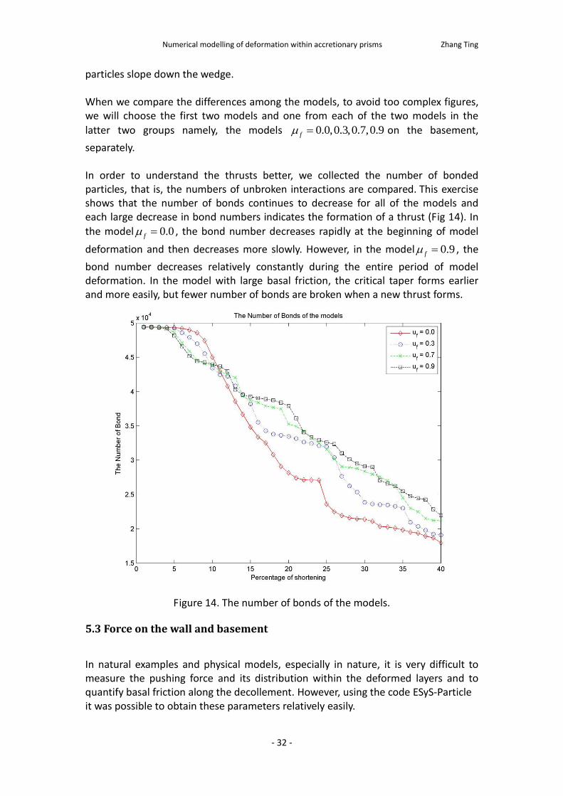
separately. In order to understand the thrusts better, we collected the number of bonded particles, that is, the numbers of unbroken interactions are compared. This exercise shows that the number of bonds continues to decrease for all of the models and each large decrease in bond numbers indicates the formation of a thrust (Fig 14). In
the model 0.0f , the bond number decreases rapidly at the beginning of model
deformation and then decreases more slowly. However, in the model 0.9f , the
bond number decreases relatively constantly during the entire period of model deformation. In the model with large basal friction, the critical taper forms earlier and more easily, but fewer number of bonds are broken when a new thrust forms.
Figure 14. The number of bonds of the models.
5.3 Force on the wall and basement
In natural examples and physical models, especially in nature, it is very difficult to measure the pushing force and its distribution within the deformed layers and to quantify basal friction along the decollement. However, using the code ESyS-Particle it was possible to obtain these parameters relatively easily.
Numerical modelling of deformation within accretionary prisms Zhang Ting
- 33 -
(a)
(b)
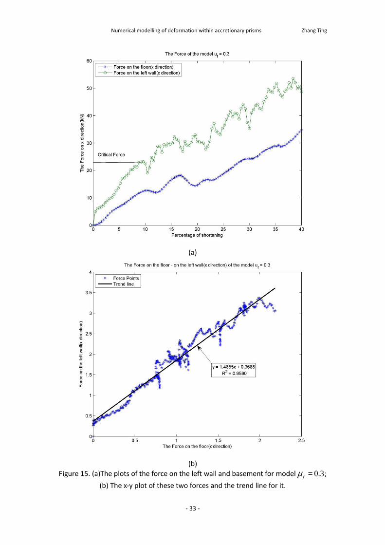
Figure 15. (a)The plots of the force on the left wall and basement for model 0.3f
m = ;
(b) The x-y plot of these two forces and the trend line for it.
Numerical modelling of deformation within accretionary prisms Zhang Ting
- 34 -
(a)
(b)
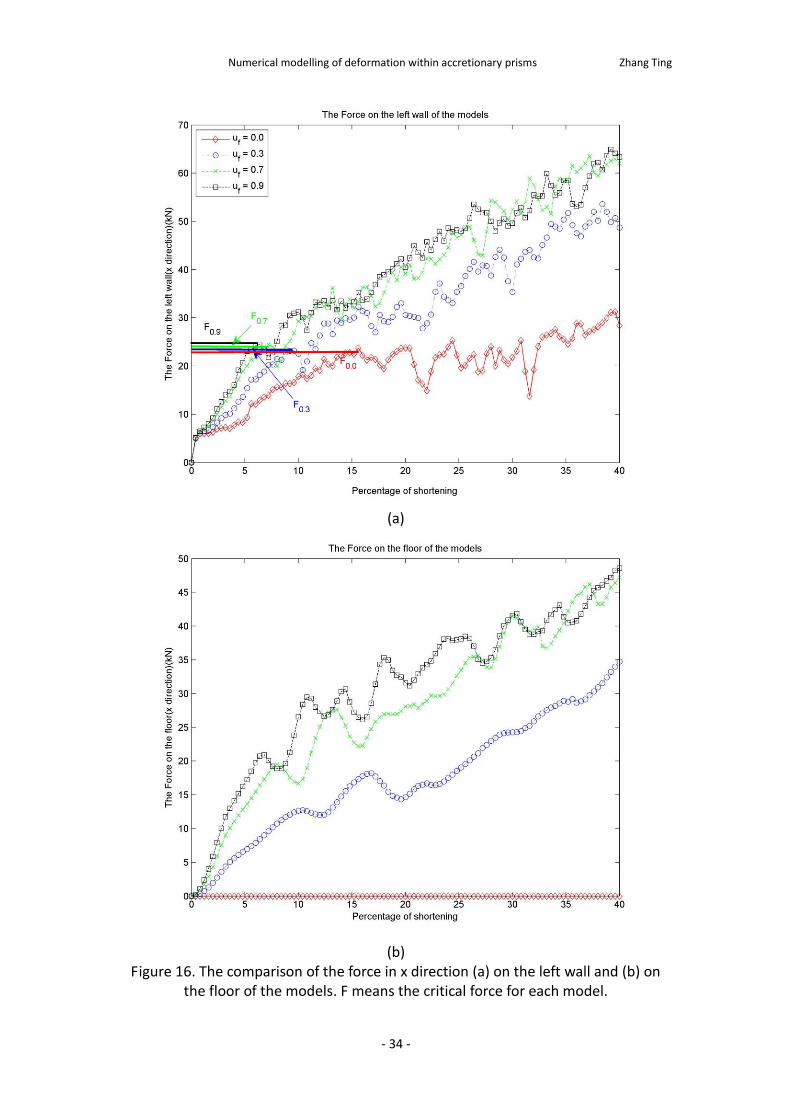
Figure 16. The comparison of the force in x direction (a) on the left wall and (b) on the floor of the models. F means the critical force for each model.
Numerical modelling of deformation within accretionary prisms Zhang Ting
- 35 -
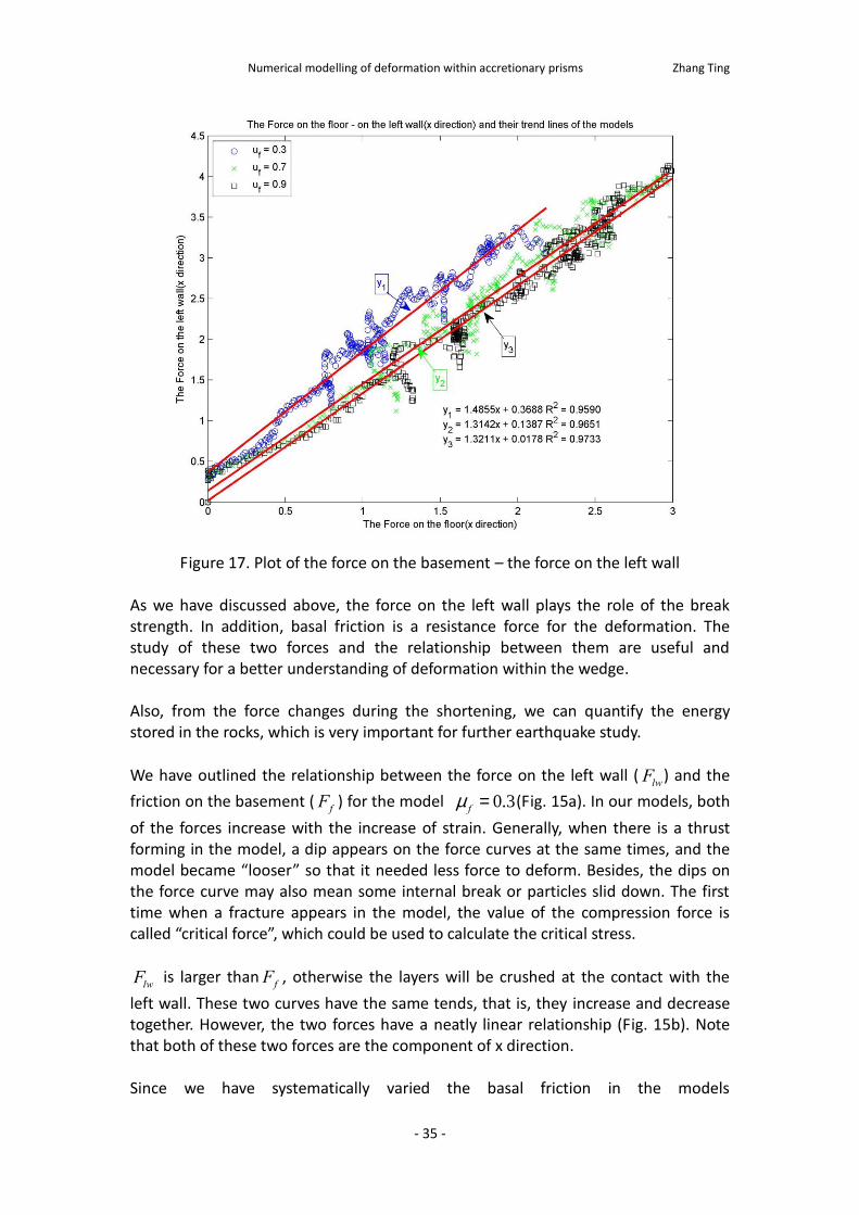
Figure 17. Plot of the force on the basement – the force on the left wall
As we have discussed above, the force on the left wall plays the role of the break strength. In addition, basal friction is a resistance force for the deformation. The study of these two forces and the relationship between them are useful and necessary for a better understanding of deformation within the wedge. Also, from the force changes during the shortening, we can quantify the energy stored in the rocks, which is very important for further earthquake study.
We have outlined the relationship between the force on the left wall (lwF ) and the
friction on the basement (fF ) for the model 0.3
fm = (Fig. 15a). In our models, both
of the forces increase with the increase of strain. Generally, when there is a thrust forming in the model, a dip appears on the force curves at the same times, and the model became “looser” so that it needed less force to deform. Besides, the dips on the force curve may also mean some internal break or particles slid down. The first time when a fracture appears in the model, the value of the compression force is called “critical force”, which could be used to calculate the critical stress.
lwF is larger thanfF , otherwise the layers will be crushed at the contact with the
left wall. These two curves have the same tends, that is, they increase and decrease together. However, the two forces have a neatly linear relationship (Fig. 15b). Note that both of these two forces are the component of x direction. Since we have systematically varied the basal friction in the models
Numerical modelling of deformation within accretionary prisms Zhang Ting
- 36 -
0.0,0.3,0.7,1.0f
m = , it was possible to compare the magnitude and distribution of
forces in different models along the left wall (Fig. 16a) and the basement (Fig. 16b). These plots show that the larger the friction is, the larger the critical force is, and a larger compression force is needed to deform the model (Fig. 16). The relationship between the two forces in different models is illustrated when they are plotted against each other (Fig. 17). The no-friction model is not plotted here because the friction is 0. It can be seen that all the trend lines for the x-y plot of the two forces are almost parallel to each other with very high degree of confidence, indicating that they are directly proportional to each other.
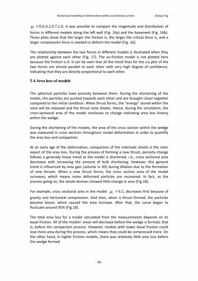
5.4 Area loss of models
The spherical particles have porosity between them. During the shortening of the model, the particles are pushed towards each other and are brought closer together compared to the initial condition. When thrust forms, the “energy” stored within the zone will be released and the thrust zone dilates. Hence, during the simulation, the cross-sectional area of the model continues to change indicating area loss history within the wedge. During the shortening of the models, the area of the cross section within the wedge was measured in cross sections throughout model deformation in order to quantify the area loss and compaction. At an early age of the deformation, compaction of the imbricate sheets is the main aspect of the area loss. During the process of forming a new thrust, porosity change follows a generally linear trend as the model is shortened, i.e., cross sectional area decreases with increasing the amount of bulk shortening. However, this general trend is influenced by area gain (volume in 3D) during dilation due to the formation of new thrusts. When a new thrust forms, the cross section area of the model increases, which means some deformed particles are recovered. In fact, as the process going on, the whole domain showed little change in area (Fig.18).
For example, cross sectional area in the model 0.3f
m = , decreases first because of
gravity and horizontal compression. And then, when a thrust formed, the particles became looser, which caused the area increase. After that, the curve began to fluctuate around 95% (Fig.18). The total area loss for a model calculated from the measurements depends on its basal friction. All of the models’ areas will decrease before the wedge is formed, that is, before the compaction process. However, models with lower basal friction could lose more area during this process, which means they could be compressed more. On the other hand, in higher friction models, there was relatively little area loss before the wedge formed.
Numerical modelling of deformation within accretionary prisms Zhang Ting
- 37 -
Figure 18. Plot of the area loss of the models After the wedge formed, the models will continue deforming so that the following process is repeated: compaction - release. Hence, the area loss will show a decrease in the compaction process and increase in the release process. It means the area loss curve will fluctuate around an “equilibrium point”. Furthermore, the value of this point is larger in high basal friction models and lower in low basal friction models. In summary, models with higher basal friction tend to have smaller amplitude and less area loss, which means that in this kind of model, particles are hard to compress. The models with lower basal friction, on the other hand, are easier to compress compared with higher basal friction models. Hence, if we fix the strain, the higher basal friction models should have more fractures.
5.5 Displacement of models
In these models, we have monitored displacement of the particles between the initial and final position. It is usually hard to measure the displacement of particles in the real world or in physical models. However, in our numerical models, the displacement of each particle could be calculated, and the displacement distribution within the wedge could be outlined. The displacement of the particles is separated into two parts, the displacement in x direction and in y direction. Hence, we can study them individually. In the past, some researchers are interested in “the displacement along individual thrust faults” (Ellis
Numerical modelling of deformation within accretionary prisms Zhang Ting
- 38 -
and Dunlap 1988), while some “measure the displacement of a certain horizon along several imbricate surfaces.”(Koyi 1995)However, in our numerical models, the initial and final position for all the particles in the models are known, which means we can easily draw a displacement distribution for all the particles.
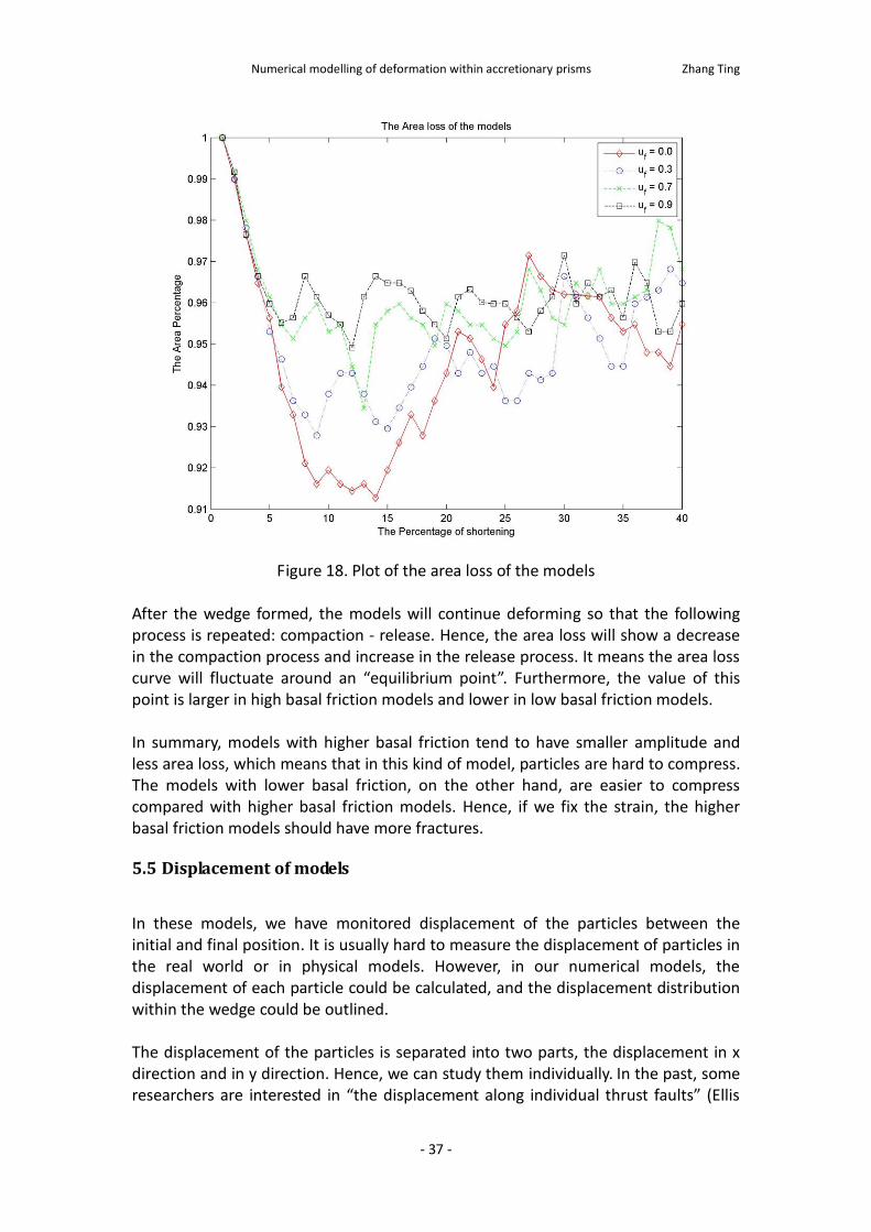
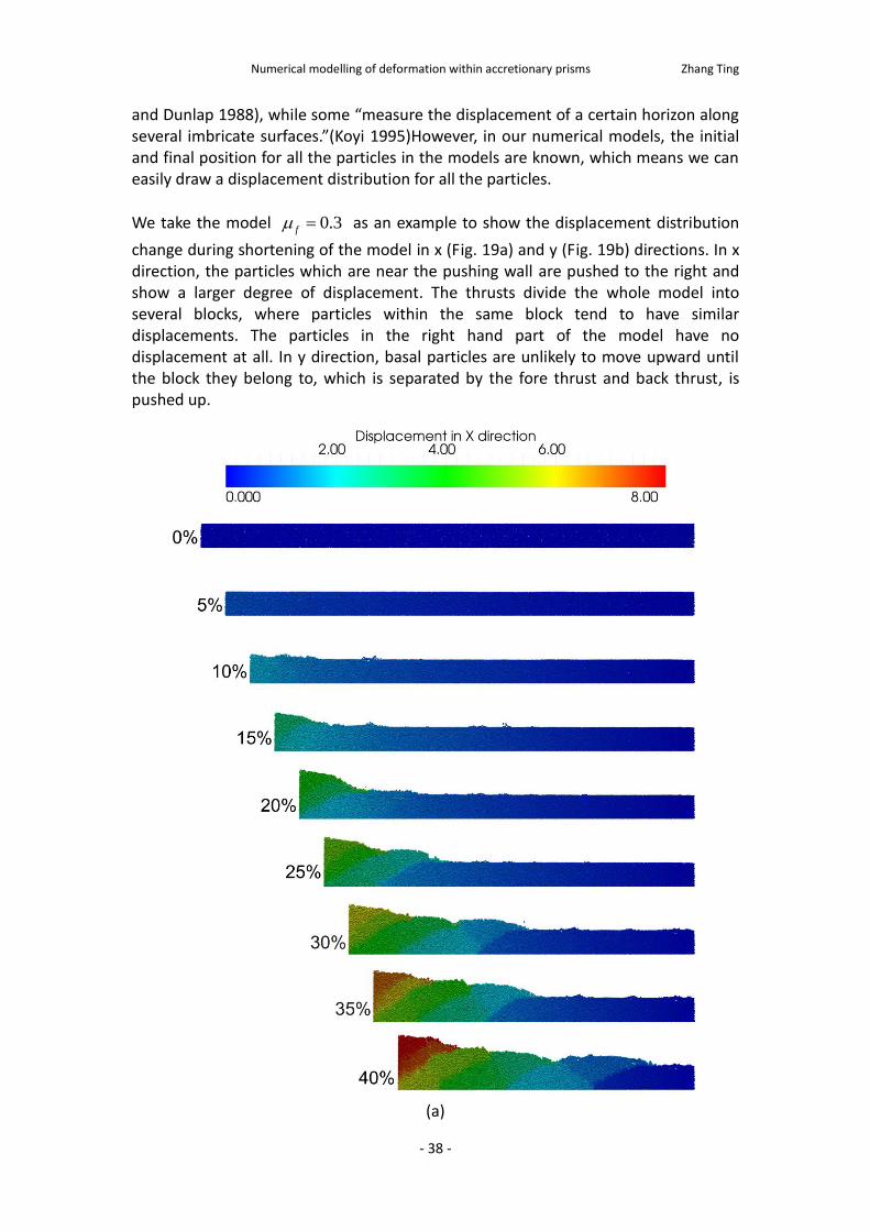
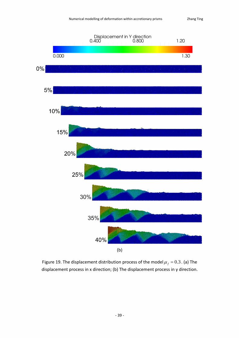
We take the model 0.3f as an example to show the displacement distribution
change during shortening of the model in x (Fig. 19a) and y (Fig. 19b) directions. In x direction, the particles which are near the pushing wall are pushed to the right and show a larger degree of displacement. The thrusts divide the whole model into several blocks, where particles within the same block tend to have similar displacements. The particles in the right hand part of the model have no displacement at all. In y direction, basal particles are unlikely to move upward until the block they belong to, which is separated by the fore thrust and back thrust, is pushed up.
(a)
Numerical modelling of deformation within accretionary prisms Zhang Ting
- 39 -
(b)
Figure 19. The displacement distribution process of the model 0.3f . (a) The
displacement process in x direction; (b) The displacement process in y direction.
Numerical modelling of deformation within accretionary prisms Zhang Ting
- 40 -
(a)
Numerical modelling of deformation within accretionary prisms Zhang Ting
- 41 -
(b)
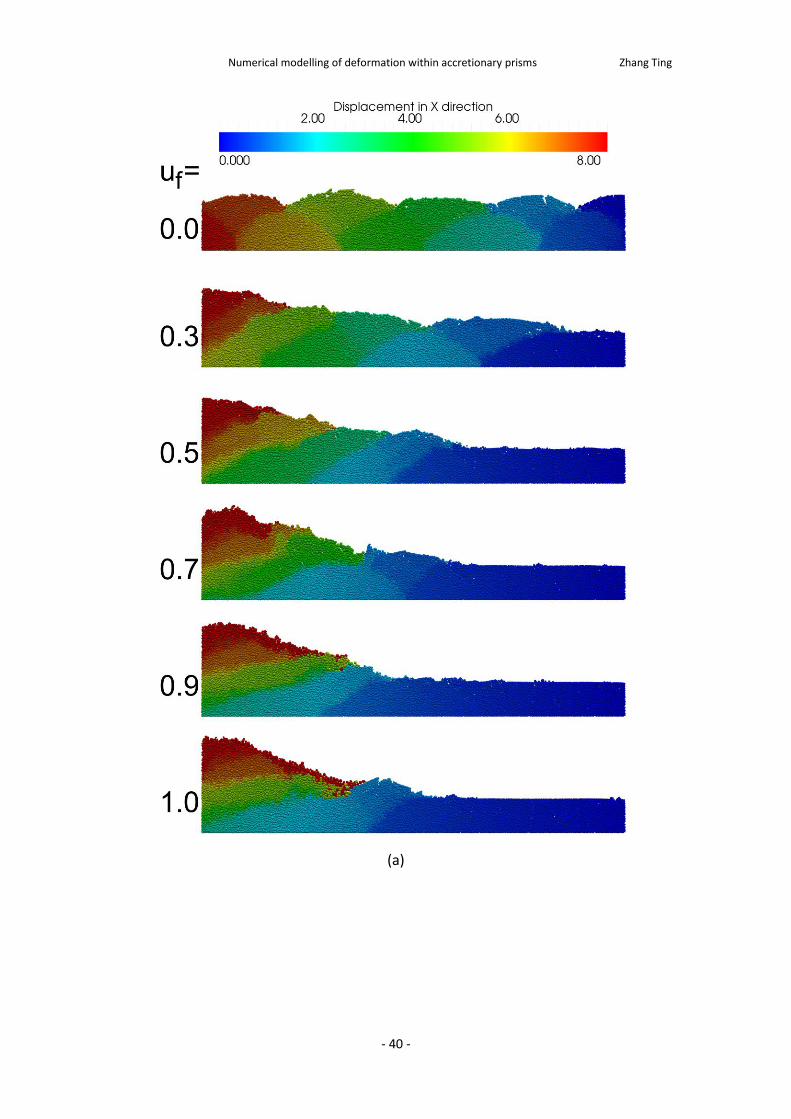
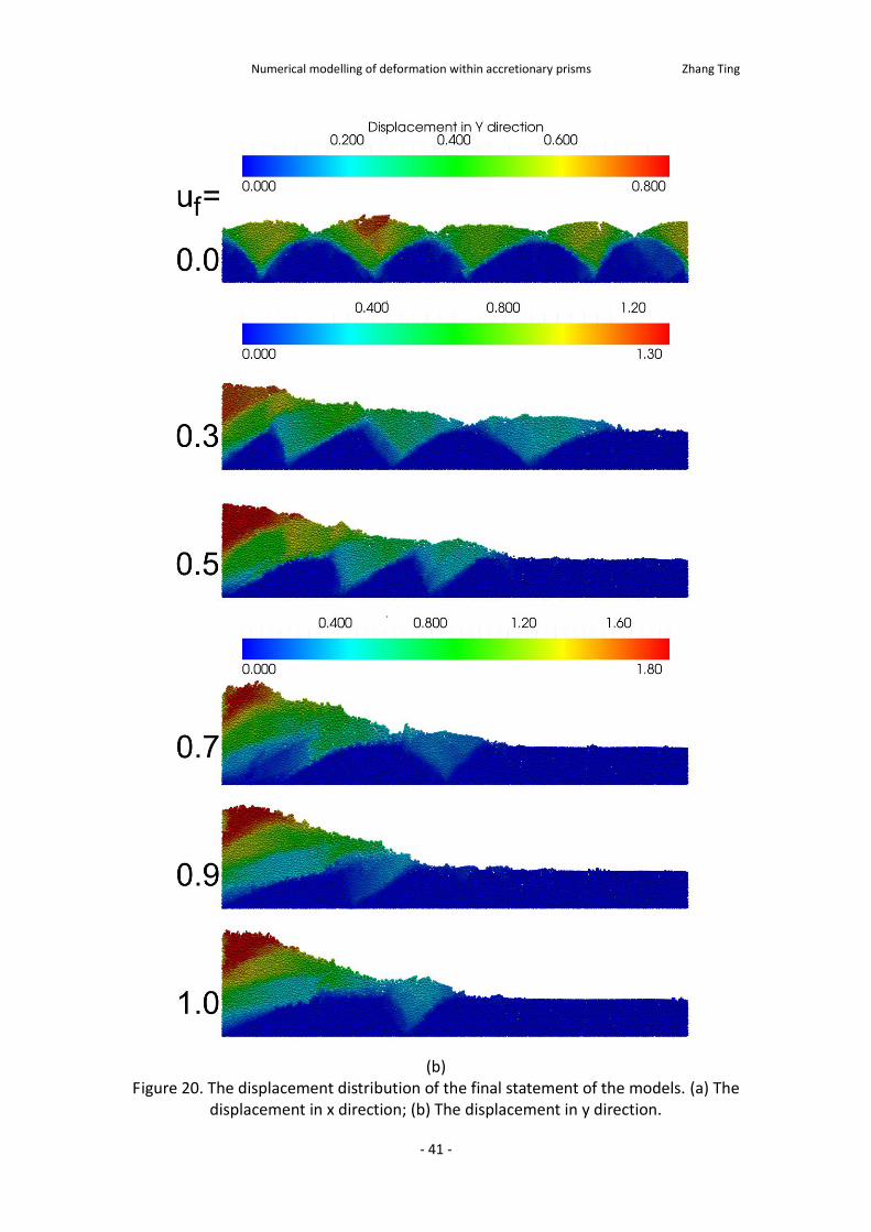
Figure 20. The displacement distribution of the final statement of the models. (a) The displacement in x direction; (b) The displacement in y direction.
Numerical modelling of deformation within accretionary prisms Zhang Ting
- 42 -
It is important to emphasise that the relative displacements of particles in x direction appear almost only in the new-formed imbricate during the shortening, while the older imbricates only move forward with the pushing wall and have almost no relative displacements. However, the situation in y direction is different. The displacements appear in the new-formed imbricate and the older imbricatesstill move upward during the process. That is to say, the displacement for the y direction is always increasing during the deformation. The final displacement distributions for x and y directions of all the six models show that basal friction governs the displacement trends in the models. In general, displacement in x direction is decreasing from the left part to the right part of the models. Displacement pattern within the model is governed by the position of the thrusts; the thrusts act as boundaries for blocks with similar displacement pattern. Within each block, particles show similar displacements both in magnitude and direction. In this way, an average value could be used to characterize the displacement of a block. With the increase of basal friction, the deformed length of the models becomes less and, when friction is too great, a slope appears (Fig. 20a). The displacement in y direction also acts as a boundary for blocks with similar displacement pattern. When the friction coefficient goes up, the height of the wedge increases. The maximal displacement of the models increases from ca. 8
(model 0.0f ) to 13 (model 5.03.0 andf ) and then up to more than 18
( 0.19.0,7.0 andf ) (Fig. 20b).
(a)
Numerical modelling of deformation within accretionary prisms Zhang Ting
- 43 -
(b)
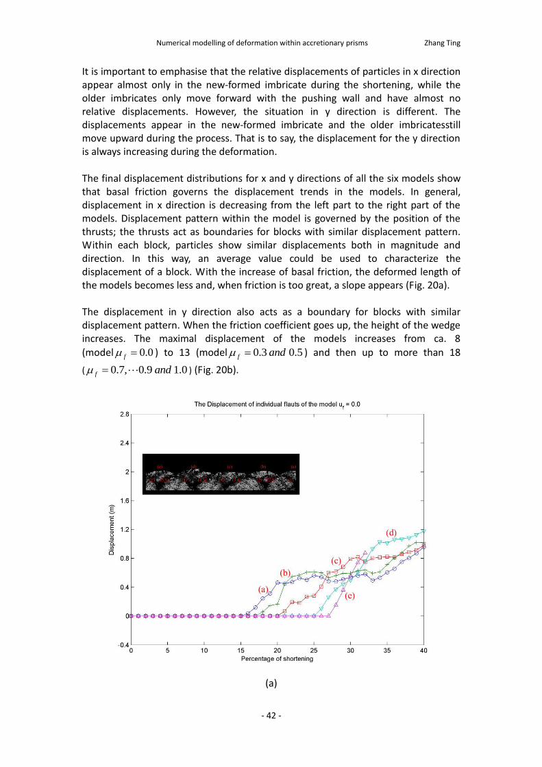
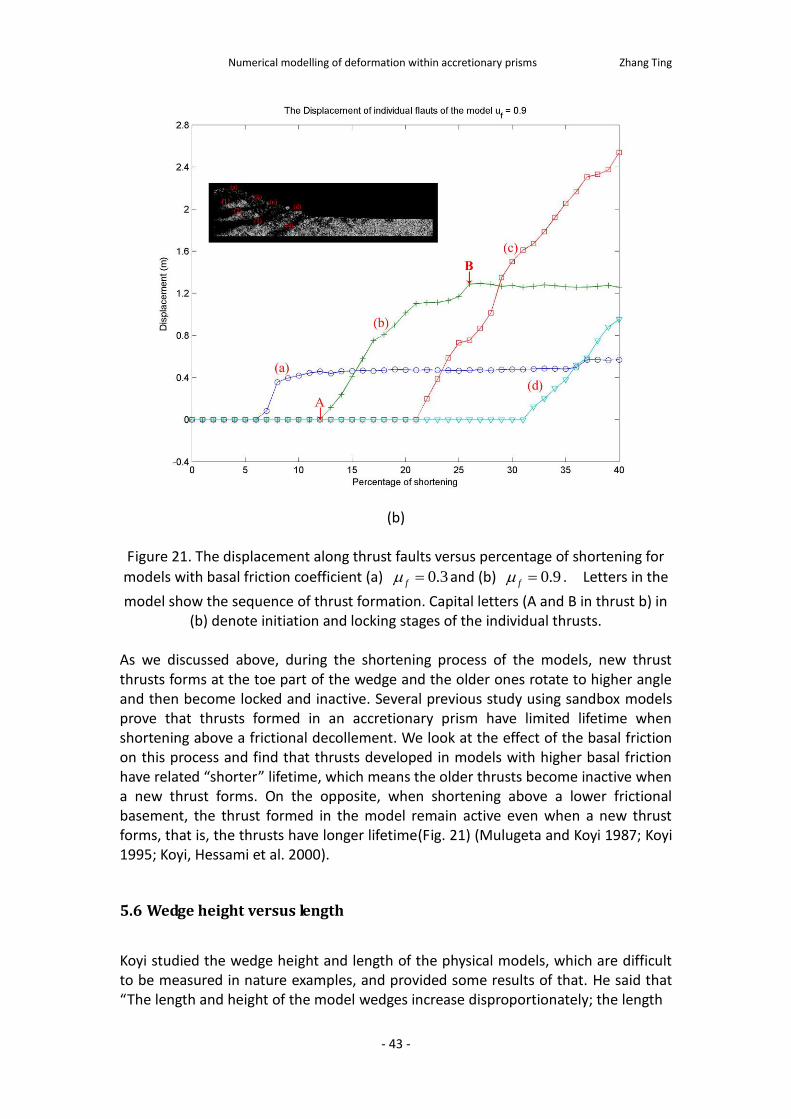
Figure 21. The displacement along thrust faults versus percentage of shortening for
models with basal friction coefficient (a) 0.3f and (b) 0.9f . Letters in the
model show the sequence of thrust formation. Capital letters (A and B in thrust b) in (b) denote initiation and locking stages of the individual thrusts.
As we discussed above, during the shortening process of the models, new thrust thrusts forms at the toe part of the wedge and the older ones rotate to higher angle and then become locked and inactive. Several previous study using sandbox models prove that thrusts formed in an accretionary prism have limited lifetime when shortening above a frictional decollement. We look at the effect of the basal friction on this process and find that thrusts developed in models with higher basal friction have related “shorter” lifetime, which means the older thrusts become inactive when a new thrust forms. On the opposite, when shortening above a lower frictional basement, the thrust formed in the model remain active even when a new thrust forms, that is, the thrusts have longer lifetime(Fig. 21) (Mulugeta and Koyi 1987; Koyi 1995; Koyi, Hessami et al. 2000).
5.6 Wedge height versus length
Koyi studied the wedge height and length of the physical models, which are difficult to be measured in nature examples, and provided some results of that. He said that “The length and height of the model wedges increase disproportionately; the length
Numerical modelling of deformation within accretionary prisms Zhang Ting
- 44 -
(a)
(b)
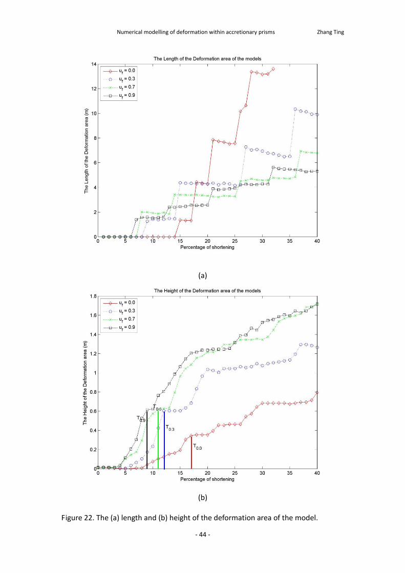
Figure 22. The (a) length and (b) height of the deformation area of the model.
Numerical modelling of deformation within accretionary prisms Zhang Ting
- 45 -
of the wedge increases episodically when each new imbricate forms, while the wedge’s height grows continually, first rapidly during the early stage of wedge formation, then much more slowly once the critical taper is reached.” (Koyi 1995) In our models, the results are measured by some numerical tools automatically, and they are similar to the physical model results. We have monitored the evolution of wedge height and length with shortening for four models shortened with different basal friction (Fig. 22). For example, in model
0.3f
m = , the height increases rapidly at first and then more gently as the wedge
establishes its critical taper. Wedge length increases sharply at first and more gently as shortening continues. However, wedge length follows an episodic evolution where it increases sharply at the formation of a new thrust and decreases gently until a new thrust forms (Fig. 22). The length may decrease after a thrust formed because of the internal compaction within the wedge and the new imbricate. Comparison between the three models with different basal friction shows that the wedge in the model with high-basal friction grew taller and shorter than in the model with low-basal friction. In the model with no basal friction, length of the deformation area is the length of the whole model after a certain percentage of shortening.
5.7 Internal Stress and Velocity
The push from the wall causes a build-up of stress in the internal part of the models. These internal stresses can show us the force distribution in the model, which could help us to find the most likely location of the next thrust and energy storage and release within the model. To make the deforming process much clearer, the internal velocity could be used to show the direction and velocity that particles tend to move in during the next step at a particular stage of the numerical simulation. However, there is a problem with drawing the stress and velocity distribution for the model. There are “special points”, where the force in the model will be focused, which means these particles are under a much larger force at certain times during the model’s deformation. The way to solve this problem is to set a value as the maximal value for the stress, and in the models, we set the critical stress to 1 by using the Mohr – Coulomb failure law for material.
Take the model 0.3f
m = for example, where the internal stress and velocity change
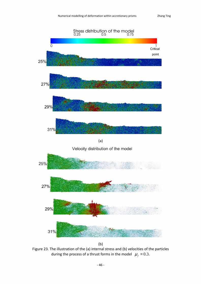
during the process of the deformation; figure 23 illustrates the internal stress and velocity distribution when a fore thrust forms. Before the new thrust generates, the stress of the particles in the model propagates
down the shortening direction and the particle velocities are consistent with this. Then, when the stress in a shear zone is larger than the critical stress, a new thrust
will form there, and the particles in this shear zone move quickly and a lot of energy is released there (25%-27% shortening). Sometimes, the back thrust forms after this
and cause energy releasing as well (27%-29% shortening). After the thrust has
Numerical modelling of deformation within accretionary prisms Zhang Ting
- 46 -
(a)
(b)
Figure 23. The illustration of the (a) internal stress and (b) velocities of the particles
during the process of a thrust forms in the model 0.3f
m = .

Numerical modelling of deformation within accretionary prisms Zhang Ting
- 47 -
formed, the stress distribution in the vicinity of the shear zone becomes inhomogeneous and compresses the new wedge horizontally to “prepare for forming the next thrust”. And the internal velocities of the particles there decrease as well (29%-31% shortening) (Fig. 23).
Numerical modelling of deformation within accretionary prisms Zhang Ting
- 48 -
6. Discussion
The discussion of the models can be separated into two main parts: firstly, discussion of the single models and secondly, discussion of comparisons among the models. In
the single model part, we take model 0.3f
m = as an example; the other models,
except model 0.0f
m = , have similar deforming histories and characteristics.
6.1 Discussion for a single model
6.1.1 Discussion of all the characteristics of the results for a single model
During the deformation of the models, certain features were common, which Koyi discussed clearly (Koyi 1995). He suggested that in the early stage, the wedge deforms internally as a complementary process because of transmitting of the compressing force overcome the basal friction, and quickly grows in order to reach a critical wedge taper. At later stage, with the continuous shortening, the wedge is compacted and rotated internally by the force transmitted from the compressing wall, which causes it become higher and longer since new thrusts will accrete in the foot of it. At the same time, some back thrusts will form inside as well. This evolution is similar to many previous models of an accretionary wedge. I quite agree with him and the evaluation of the models shows the same results (Fig. 12 & 14). The pushing force from the left wall is similar to the description of the forming of imbricates above. Firstly, it increases very quickly to reach a value which is the critical point of forming a thrust. Then, its growth becomes gentler to push the model forward (Fig. 15a). In our study, the area loss is based on the compression until the model reaches the critical taper. Hence, at an early stage, the cross sectional area decreases rapidly. After this process, however, the area of the cross section shows gentler decrease because of the internal compaction until new imbricate forms. When a new imbricate is added to the deformed triangle domain or a back thrust forms, the area of the cross section shows a slightly increase because of the compaction of the break parts. In general, the area loss of the cross section for the models is around 5-7%. For the size of the model wedge, it grows both in length and height during the shortening process. At the early stage, a rapid growth of the wedge continues until a critical taper is reached. After that, however, the changes in length and height of the deformed wedge are different. The height of the wedge increases gently in small steps, while the length of the deformation area displays episodes of sudden change
Numerical modelling of deformation within accretionary prisms Zhang Ting
- 49 -
when younger imbricates are accreted. (Fig. 21) As expected, each of these steps predates the formation of a new imbricate. (Koyi 1995) After all, the process of forming a new imbricate can be described as follow. Firstly, the wedge is getting thick under the compressing force over the basal friction until the system reach a critical statement again. Then a new thrust forms and slips along the decollement. Any slightly change of the boundary conditions will significantly change this critical statement geometry of the resulting wedges. In this paper, as we said above, we focus on the basal friction and other parameters will be discussed later.
6.1.2 Results versus Evolution of the model
After comparing the number of bonds, force, area loss, displacement and height versus length of the model, it is clear that when a new imbricate appears, all of the characteristics within the wedge will change correspondingly to make sure that the force can be transferred to the undeformed area and the model evolution can reach other critical tapers. The cycling of this process leads to the final statement of the model. The most essential parts of the deformation are the forming of the thrusts and their slipping. If a fore thrust has a back thrust, they form continuously which means they almost form at the same time. A fore thrust slips while it forms, however, a back thrust slips some time later. The value change of the characteristics during the process is based the thrust forming and slipping.
Take the model 0.3f
m = for example; there are five fore trusts and four back
thrusts. However, the second and third fore thrusts and their back thrust almost form at the same time so they are treated as a single, large deforming process. All of these characteristics are consistent with the deformation process. The compression force continuous increases during the process, and it shows a decrease when a thrust is forming or slipping; Conversely, the area of the cross section of the model decreases during the shortening because of compaction, and increases when a thrust is forming or slipping; When the size of the deforming area is considered, the height of it continues to increase during the whole process, while the length of the deforming area enlarges dramatically when a fore thrust forms and almost remains the same, even when a back thrust is happening; A large number bonds in the model begin to break to “prepare” for a thrust and this process continuous until the thrust stop slipping, that is, the system is balance (Fig. 24).
6.2 Comparison of models
As we see above, the number of imbricates forming depends on the mechanical properties of the shortened layers and on the basal friction. Our models show that basal friction governs the spacing and size of imbricates formed in the shortened
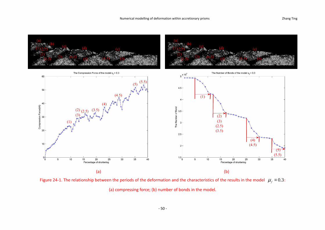
Numerical modelling of deformation within accretionary prisms Zhang Ting
- 50 -
(a) (b)
Figure 24-1. The relationship between the periods of the deformation and the characteristics of the results in the model 0.3f
m = :
(a) compressing force; (b) number of bonds in the model.
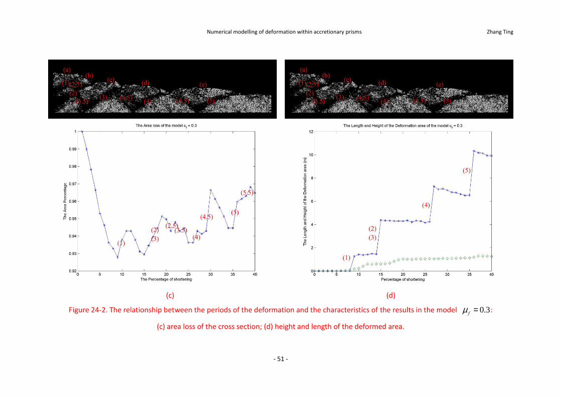
Numerical modelling of deformation within accretionary prisms Zhang Ting
- 51 -
(c) (d)
Figure 24-2. The relationship between the periods of the deformation and the characteristics of the results in the model 0.3f
m = :
(c) area loss of the cross section; (d) height and length of the deformed area.
Numerical modelling of deformation within accretionary prisms Zhang Ting
- 52 -
models. Imbricates formed above a high-friction basement are more numerous, have irregular spacing, and are of different sizes, whereas those formed above a low- friction basement are fewer, have relatively regular spacing, and are in general of similar size (Fig. 14 & 12). Besides the number of imbricates, basal friction also influences displacement magnitude and distribution, and height and length of the deformed area. Similar to the previous studies, comparison between the six models with different basal frictions shows that the higher basal friction models tend to has taller, shorter and steeper wedges. In addition, in a low friction models, the increasing rate of the pushing force is low. On the other hand, in high friction models, the situation is the opposite. (Fig. 19 & 22) “In nature, fluid overpressure can alter basal friction drastically and is capable of reducing the strength of the decollement by 90% or more.” (Koyi and Vendeville 2003) Consequently, changing basal friction is likely to have a great impact on the results. (Schopfer, Arslan et al. 2011) The results show that a model or natural example with a higher basal friction may have a smaller deformation area. That is to say, the model is more stable and less energy can be stored there. On the other hand, low-basal friction models are easier to deform and seem to have larger energy release when a thrust is forming. Previous study of the physical models has shown that the geometry of models with higher basal friction tends to be steeper, taller and shorter. (Koyi and Vendeville 2003). And the results of the models proved that. The study of area loss of the models with different friction shows that area loss is related to the basal friction. The area loss for a model with higher friction on the basement tends to have less area loss and smoother fluctuation around a related larger equilibrium point, while the lower friction models have larger area loss and higher volatility around a lower equilibrium point (Fig. 18). Especially when there is no basal friction, because the stain rate is small, the stress can transfer into the whole model under the shortening force with no damping, and the geometry of the model will present several symmetrical wedges.
Numerical modelling of deformation within accretionary prisms Zhang Ting
- 53 -
7. Conclusion
Results from the DEM models shortened with different basal frictions show that: For a single model, in the early stage, the wedge deforms internally as a complementary process because of transmitting of the compressing force overcome the basal friction, and quickly grows in order to reach a critical wedge taper. After that, several characteristics change under the pushing force: the pushing force and friction grow gentler to push the model forward; the crossing area increases rapidly when a new thrust is forming and decreases smoothly during compacting; the relative displacements almost all happen in the new deforming area and for the older imbricates are almost zero, and the absolute displacements increase at a constant rate; wedges grow both in height and length with progressive shortening. Additionally, all of these behaviours are consistent with the process of forming a new thrust. The internal stress plays an important role when a new thrust forms. The shear zone where the stress is larger than the critical stress is the area of a new thrust formation. And after the new thrust forms, the internal stress is released. During this process, the internal velocities of particles indicate the direction and amount of the tendency for break and slip. The results of comparison of models illustrate that basal friction has a significant influence on the wedges’ geometry and kinematics.
1. In general, model results show a steeper taper wedge and have gentler fore thrusts when shortened above a high-friction basement. And higher friction models have less back thrusts.
2. Then the compressing force is higher when the basal friction is larger, and the trend lines for the x-y plot of the two forces are almost parallel to each other.
3. The area loss for a model with higher friction on the basement tends to have less area loss and smoother fluctuation around a related larger equilibrium point.
4. In general, with the same amount of bulk shortening, the height of wedges formed above a higher friction basement is larger than wedges shortened above a lower friction basement; while the length of wedge is smaller.
5. In a high basal friction model, displacement on individual thrusts is higher. Older thrusts have longer lifetime.
6. Especially, when there is no basal friction, several symmetrical wedges will form and
they distribute evenly within the whole length of the model.
Numerical modelling of deformation within accretionary prisms Zhang Ting
- 54 -
8. Acknowledgements
In writing this thesis, I greatly appreciate the guidance and supervision from my supervisor Prof. Hemin Koyi, and thank him for his understanding and tolerance. Without his help, this paper could not have been finished. Thanks to the contributor of the software Dr. Dion Weatherley, for kindly and patiently answering my questions about the project and software. Thanks to the coordinator Michael Thuné and director of studies Stefan Pålsson, for all they have done for us during these two years. In this two-year study, my biggest asset is the best friends I have got to know through living and learning. Here, I express my sincere gratitude to them. Thanks to my thesis review Maya Neytcheva, she spends lot of time helping me correcting my writing. Thanks to my parents, without their care and support there would be no me today. At this moment, I shall give the highest respects to them! In this paper, I referenced a large number of documents; here, I will give thanks to all these great scientists.
Numerical modelling of deformation within accretionary prisms Zhang Ting
- 55 -
9. References
Weatherley, D. and Boros, V. "ESyS-Particle v2.0 user's guide", Earth Systems Science Computational Centre, The University of Queensland, Australia, 2009
Abe, S. "The Discrete Element Method as implemented in ESyS-Particle - Background and some Theory", GED, RWTH, 2009
Lei Tian and Haijian Ye, “Studies of Parallel Computing Based on the Cluster and Applications in Discrete Element Computation”, Mastere Thesis, China Agricultural University, 2006
Abe, S. (2009). "The Discrete Element Method as implemented in ESyS-Particle - Background and some Theory." GED, RWTH.
Abe, S., D. Place, et al. (2004). "A parallel implementation of the lattice solid model for the simulation of rock mechanics and earthquake dynamics." Pure and Applied Geophysics 161(11-12): 2265-2277.
Cundall, P. A. and O. D. L. Strack (1979). "Discrete Numerical-Model for Granular Assemblies." Geotechnique 29(1): 47-65.
Johnson, K. L. (1985). Contact mechanics. Cambridge Cambridgeshire ; New York, Cambridge University Press.
Koyi, H. (1991). "Gravity Overturns, Extension, and Basement Fault Activation." Journal of Petroleum Geology 14(2): 117-142.
Koyi, H. (1995). "Mode of Internal Deformation in Sand Wedges." Journal of Structural Geology 17(2): 293-&.
Koyi, H. A., K. Hessami, et al. (2000). "Epicenter distribution and magnitude of earthquakes in fold-thrust belts: insights from sandbox models." Geophysical Research Letters 27(2): 273-276.
Koyi, H. A. and B. C. Vendeville (2003). "The effect of decollement dip on geometry and kinematics of model accretionary wedges." Journal of Structural Geology 25(9): 1445-1450.
Mindlin, R. D. and H. Deresiewicz (1953). "Elastic Spheres in Contact under Varying Oblique Forces." Journal of Applied Mechanics-Transactions of the Asme 20(3): 327-344.
Mora, P. and D. Place (1994). "Simulation of the Frictional Stick-Slip Instability." Pure and Applied Geophysics 143(1-3): 61-87.
Mora, P. and D. Place (2002). "Stress correlation function evolution in lattice solid elasto-dynamic models of shear and fracture zones and earthquake prediction." Pure and Applied Geophysics 159(10): 2413-2427.
Mulugeta, G. and H. Koyi (1987). "3-Dimensional Geometry and Kinematics of Experimental Piggyback Thrusting." Geology 15(11): 1052-1056.
Mulugeta, G. and H. Koyi (1992). "Episodic Accretion and Strain Partitioning in a Model Sand Wedge." Tectonophysics 202(2-4): 319-333.
Place, D. and P. Mora (1999). "The lattice solid model to simulate the physics of rocks and earthquakes: Incorporation of friction." Journal of Computational Physics 150(2): 332-372.
Poschel, T. and T. Schwager (2005). Computational granular dynamics : models and algorithms. Berlin ; New York, Springer-Verlag.
Potyondy, D. O. and P. A. Cundall (2004). "A bonded-particle model for rock." International Journal of Rock Mechanics and Mining Sciences 41(8): 1329-1364.
Schopfer, M. P. J., S. Abe, et al. (2009). "The impact of porosity and crack density on the elasticity, strength and friction of cohesive granular materials: Insights from DEM modelling." International Journal of Rock Mechanics and Mining Sciences 46(2): 250-261.
Schopfer, M. P. J., A. Arslan, et al. (2011). "Reconciliation of contrasting theories for fracture spacing in layered rocks." Journal of Structural Geology 33(4): 551-565.
Simpson, G. (2011). "Mechanics of non-critical fold-thrust belts based on finite element models." Tectonophysics 499(1-4): 142-155.
Storti, F. and K. Mcclay (1995). "Influence of Syntectonic Sedimentation on Thrust Wedges in Analog

Numerical modelling of deformation within accretionary prisms Zhang Ting
- 56 -
Models." Geology 23(11): 999-1002. Storti, F., F. Salvini, et al. (1997). "Fault-related folding in sandbox analogue models of thrust wedges."
Journal of Structural Geology 19(3-4): 583-602. Weatherley, D. and V. Boros (2009). "ESyS-Particle v2.0 user's guide." Earth Systems Science
Computational Centre, The University of Queensland, Australia.