numerical modelling of mining subsidence upsidence and valley closure using udec
DESCRIPTION
thesis on mine subsidenceTRANSCRIPT

NUMERICAL MODELLING OF MINING SUBSIDENCE,
UPSIDENCE AND VALLEY CLOSURE USING UDEC
A thesis submitted in fulfillment of the
requirements for the award of the degree
DOCTOR OF PHILOSOPHY
from
UNIVERSITY OF WOLLONGONG
by
Walter Keilich, BE Hons (Mining)
SCHOOL OF CIVIL, MINING AND ENVIRONMENTAL
ENGINEERING
2009
Thesis Certification
i
THESIS CERTIFICATION
I, Walter Keilich, declare that this thesis, submitted in fulfilment of the requirements for
the award of Doctor of Philosophy, in the School of Civil, Mining and Environmental
Engineering, University of Wollongong, is wholly my own work unless otherwise
referenced or acknowledged below. The document has not been submitted for
qualifications at any other academic institution.
Walter Keilich
9/09/2009
Table Of Contents
ii
TABLE OF CONTENTS
CHAPTER TITLE PAGE
THESIS CERTIFICATION i
TABLE OF CONTENTS ii
LIST OF FIGURES vii
LIST OF TABLES xiv
LIST OF SYMBOLS xvi
ABSTRACT xviii
ACKNOWLEDGEMENTS xx
PUBLICATIONS ARISING FROM RESEARCH PROJECT xxii
1 INTRODUCTION 1
1.1 PROBLEM STATEMENT AND OBJECTIVE 1
1.2 METHODOLOGY 3
1.3 OUTCOMES AND POTENTIAL APPLICATIONS 4
2 MINE SUBSIDENCE IN THE SOUTHERN COALFIELD 5
2.1 INTRODUCTION 5
2.2 SUBSURFACE MOVEMENT 6
2.2.1 Zones of movement in the overburden 7
2.2.2 Caving in the Southern Coalfield and its
significance on subsidence development 8
2.3 SURFACE DEFORMATIONS 9
2.3.1 Angle of draw 13
2.3.2 Extraction area 14
2.3.3 Stationary and dynamic subsidence profiles 16
2.4 SOUTHERN COALFIELD GEOLOGY 17
2.4.1 The Sydney Basin 17
2.4.2 The Southern Coalfield 19
2.4.2.1 Illawarra Coal Measures 20
2.4.2.2 Narrabeen Group 26

Table Of Contents
iii
2.4.2.3 Hawkesbury Sandstone 29
2.5 CURRENT PREDICTION TECHNIQUES USED IN
THE SOUTHERN COALFIELD 29
2.5.1 New South Wales Department of Primary
Industries Empirical Technique 30
2.5.1.1 Overview of method 30
2.5.1.2 Maximum developed subsidence for
single longwall panels 32
2.5.1.3 Maximum developed subsidence for
multiple longwall panels 33
2.5.1.4 Maximum strains 36
2.5.1.5 Maximum tilt 37
2.5.1.6 Radius of ground curvature 38
2.5.1.7 Location of inflection point 38
2.5.1.8 Goaf edge subsidence 39
2.5.2 The Incremental Profile Method 40
2.5.2.1 Overview of method 40
2.6 SUMMARY 45
3 VALLEY CLOSURE AND UPSIDENCE 47
3.1 INTRODUCTION 47
3.2 CURRENT MODELS 49
3.2.1 Horizontal stress model 49
3.2.2 Empirical predictions 51
3.2.3 Limitations 62
3.2.4 Recent developments 64
3.3 ALTERNATIVE MODEL 65
3.3.1 Kinematics of a particle moving along a known
path 67
3.3.2 Adaptation to blocks moving along a known path 72
3.4 REQUIRED WORK PROGRAM 77
3.5 SUMMARY 77
Table Of Contents
iv
4 DEVELOPMENT OF A NUMERICAL MODELLING
APPROACH 78
4.1 INTRODUCTION 78
4.2 MODELLING PRINCIPLES 78
4.3 LITERATURE REVIEW 79
4.3.1 Coulthard and Dutton (1988) 79
4.3.2 Johansson, Riekkola and Lorig (1988) 80
4.3.3 Alehossein and Carter (1990) 80
4.3.4 Brady et al. (1990) 81
4.3.5 Choi and Coulthard (1990) 82
4.3.6 O’Conner and Dowding (1990) 83
4.3.7 Coulthard (1995) 84
4.3.8 Bhasin and Høeg (1998) 85
4.3.9 Alejano et al. (1999) 86
4.3.10 Sitharam and Latha (2002) 88
4.3.11 CSIRO Petroleum (2002) 89
4.4 SUMMARY 90
5 SINGLE LONGWALL PANEL MODELS WITH NO RIVER
VALLEY 92
5.1 INTRODUCTION 92
5.2 NUMERICAL MODELLING STRATEGY 92
5.3 MATERIAL PROPERTIES FOR INTACT ROCK 93
5.4 PROPERTIES OF THE BEDDING DISCONTINUITIES 99
5.5 VERTICAL JOINTS AND PROPERTIES 101
5.6 IN-SITU STRESS 103
5.7 MESH GENERATION 104
5.8 CONSTITUTIVE MODELS 106
5.9 BOUNDARY CONDITIONS 106
5.10 HISTORIES 106
5.11 MODEL GEOMETRY AND INITIAL TEST MODELS 106
5.12 RESULTS 117
5.13 SUMMARY 156

Table Of Contents
v
6 SINGLE LONGWALL PANEL MODELS WITH RIVER
VALLEY 157
6.1 INTRODUCTION 157
6.2 MODELLING STRATEGY 157
6.3 INITIAL MODELS AND MESH DENSITY ANALYSIS 158
6.4 RIVER VALLEY MODELS 178
6.5 RESULTS 187
6.5.1 Subsidence without valley excavation 189
6.5.2 Tilt without valley excavation 193
6.5.3 Subsidence/upsidence at base of valleys 196
6.5.4 Valley closure at shoulders 208
6.5.5 Valley closure at base 218
6.5.6 Valley base yield 221
6.6 COMPARISON TO EMPIRICAL DATA 226
6.7 PARAMETRIC STUDY 240
6.8 COMPARISON TO BLOCK KINEMATICS 245
6.9 SUMMARY 248
7 APPLICATION OF VOUSSOIR BEAM AND PLATE
BUCKLING THEORY 250
7.1 INTRODUCTION 250
7.2 APPLICATION OF VOUSSOIR BEAM THEORY 250
7.3 APPLICATION OF PLATE BUCKLING THEORY 252
7.4 SUMMARY 253
8 SUMMARY, CONCLUSIONS AND RECOMMENDATIONS 256
8.1 SUMMARY 256
8.1.1 Review of problem 256
8.1.2 The block movement model 257
8.1.3 Numerical modelling 258
8.1.4 Application of analytical solutions 260
8.2 CONCLUSIONS 260
8.3 LIMITATIONS OF THE STUDY 261
8.4 RECOMMENDATIONS 262

Table Of Contents
vi
LIST OF REFERENCES 264
APPENDIX A 273
APPENDIX B 288
APPENDIX C 302
APPENDIX D 327
APPENDIX E 352

List Of Figures
vii
LIST OF FIGURES
FIGURE TITLE PAGE
1.1 Water level reduction in river valley affected by longwall mining 2
1.2 Unsightly cracking of rock bars in river valley affected by
longwall mining 2
2.1 Relationship between panel width, goaf angle and effective span 6
2.2 Overburden movement above a longwall panel 7
2.3 Cross section of longwall panel with microseismic event location 9
2.4 Characteristics of trough subsidence 12
2.5 Sub-critical, critical and super-critical trough shapes 15
2.6 Stationary subsidence profiles 16
2.7 Dynamic subsidence profiles 16
2.8 Idealised stratigraphic column of the Southern Coalfield 20
2.9 Formation of a subsidence trough above an extraction panel 31
2.10 Relationship between W/H ratio and Smax/T for single panels 32
2.11 Relationship between W/H and Smax/T for multiple panels 34
2.12 Relationship between pillar stress factor (WLH/PW) and Smax/T
for multiple panel layouts 35
2.13 Relationship between W/H ratio and K1 36
2.14 Relationship between W/H ratio and K2 37
2.15 Relationship between W/H ratio and K3 37
2.16 Relationship between maximum strain and minimum radius of
curvature 38
2.17 Location of inflection point 39
2.18 Goaf edge subsidence 39
2.19 Typical incremental subsidence profiles, NSW Southern Coalfield 41
2.20 Incremental subsidence profiles obtained using the Incremental
Profile Method 43
2.21 Prediction curves for maximum incremental subsidence 43

List Of Figures
viii
3.1 Buckling of rock bars resulting in low angle fractures 47
3.2 Buckling of rock bars leading to vertical cracks 48
3.3 Reduction in creek water level due to mining 48
3.4 Notch effect on horizontal stress field 50
3.5 Strata buckling mechanism due to in-situ horizontal stress 50
3.6 Possible failure mechanisms in the bottom of a valley 51
3.7 Distance measurement convention for valley closure and
upsidence predictions 52
3.8 Valley closure versus transverse distance from the advancing goaf
edge 54
3.9 Valley closure adjustment factor versus longitudinal distance 55
3.10 Valley closure adjustment factor versus valley depth 56
3.11 Valley closure adjustment factor versus maximum incremental
subsidence 57
3.12 Upsidence versus transverse distance from the advancing goaf
edge 58
3.13 Upsidence adjustment factor versus longitudinal distance 59
3.14 Upsidence adjustment factor versus valley depth 60
3.15 Upsidence adjustment factor versus maximum incremental
subsidence 61
3.16 Original and amended plan for mining near the Nepean River 63
3.17 New conceptual model for upsidence and valley closure in the
hogging phase 66
3.18 Position 68
3.19 Radius of curvature 68
3.20 Velocity 69
3.21 Time derivative 70
3.22 Time derivative components 70
3.23 Acceleration 72
3.24 Magnified block displacements on curved slope 73
3.25 Area of contact between rotating blocks 73
3.26 Length of an arc 74
3.27 Exaggerated view of valley tilt and resulting closure 75
3.28 Components of valley tilt 75

List Of Figures
ix
5.1 Typical mesh configuration for all models 105
5.2 Thickness of stratigraphic units grouped according to mine 110
5.3 Model 1 geometry 112
5.4 Model 2 geometry 113
5.5 Model 3 geometry 114
5.6 Model 4 geometry 115
5.7 Subsidence profiles for different damping options 116
5.8 Superimposed model results for Smax/T 119
5.9 Superimposed model results for Sgoaf/Smax 120
5.10 Superimposed model results for K1 121
5.11 Superimposed model results for K2 122
5.12 Superimposed model results for K3 123
5.13 Superimposed model results for D/H 124
5.14 Development of maximum subsidence in Model 1 127
5.15 Subsidence profile for Model 1 128
5.16 Strain profile for Model 1 129
5.17 Tilt profile for Model 1 130
5.18 Yielded zones and caving development in Model 1 131
5.19 Detailed view of yielded zones in Model 1 132
5.20 Yielded zones and joint slip in Model 1 133
5.21 Development of maximum subsidence in Model 2 134
5.22 Subsidence profile for Model 2 135
5.23 Strain profile for Model 2 136
5.24 Tilt profile for Model 2 137
5.25 Yielded zones and caving development in Model 2 138
5.26 Detailed view of yielded zones in Model 2 139
5.27 Yielded zones and joint slip in Model 2 140
5.28 Development of maximum subsidence in Model 3 141
5.29 Subsidence profile for Model 3 142
5.30 Strain profile for Model 3 143
5.31 Tilt profile for Model 3 144
5.32 Yielded zones and caving development in Model 3 145
5.33 Detailed view of yielded zones in Model 3 146
5.34 Yielded zones and joint slip in Model 3 147

List Of Figures
x
5.35 Development of maximum subsidence in Model 4 148
5.36 Subsidence profile for Model 4 149
5.37 Strain profile for Model 4 150
5.38 Tilt profile for Model 4 151
5.39 Yielded zones and caving development in Model 4 152
5.40 Detailed view of yielded zones in Model 4 153
5.41 Yielded zones and joint slip in Model 4 154
6.1 Y-displacements on the surface and at the base of various rock
units 161
6.2 Geometry of initial river valley models 163
6.3 Finite different zoning used in valley models 164
6.4 Vertical displacements at base of Bulgo Sandstone 166
6.5 Subsidence profile comparison for varying cycles (N) 167
6.6 Yielded zones for N = 30,000 cycles 168
6.7 Model with bedding in upper 70 m of Hawkesbury Sandstone 170
6.8 Model with bedding and joints in upper 70 m of Hawkesbury
Sandstone 171
6.9 Subsidence profile comparison for bedding and joints 172
6.10 Yielded zones in a river valley model with bedding 173
6.11 Yielded zones in a river valley model with bedding and joints 174
6.12 Beam buckling in Model 7 176
6.13 Beam buckling in Model 8 177
6.14 Typical river valley model 181
6.15 Translation plane at base of valley 182
6.16 Translation plane below base of valley 183
6.17 Translation plane at base of valley (bedding and joints) 184
6.18 Translation plane below base of valley (bedding and joints) 185
6.19 Translation plane below base of valley (joints in beam) 186
6.20 Subsidence prior to valley excavation (no bedding and joints in
upper 70 m of Hawkesbury Sandstone) 191
6.21 Subsidence prior to valley excavation (bedding and joints in upper
70 m of Hawkesbury Sandstone) 192

List Of Figures
xi
6.22 Tilt prior to valley excavation (no bedding and joints in upper
70 m of Hawkesbury Sandstone) 194
6.23 Tilt prior to valley excavation (bedding and joints in upper 70 m
of Hawkesbury Sandstone) 195
6.24 Subsidence at base (no bedding and joints in upper 70 m of
Hawkesbury Sandstone) 199
6.25 Exaggerated block deformations when valley is 0 m from
longwall centreline (no bedding and joints in upper 70 m of
Hawkesbury Sandstone) 200
6.26 Exaggerated block deformations when valley is 50 m from
longwall centreline (no bedding and joints in upper 70 m of
Hawkesbury Sandstone) 201
6.27 Exaggerated block deformations when valley is 100 m from
longwall centreline (no bedding and joints in upper 70 m of
Hawkesbury Sandstone) 202
6.28 Block deformations and shear when valley is 0 m from longwall
centreline (no bedding and joints in upper 70 m of Hawkesbury
Sandstone, joints in beam) 203
6.29 Subsidence at base (bedding and joints in upper 70 m of
Hawkesbury Sandstone) 204
6.30 Block deformation and shear when valley is 100 m from longwall
centreline (bedding and joints in upper 70 m of Hawkesbury
Sandstone) 205
6.31 Horizontal stress when valley is 100 m from longwall centreline
(no bedding and joints in upper 70 m of Hawkesbury Sandstone) 206
6.32 Horizontal stress when valley is 100 m from longwall centreline
(bedding and joints in upper 70 m of Hawkesbury Sandstone) 207
6.33 Valley closure at shoulders (no bedding and joints in upper 70 m
of Hawkesbury Sandstone) 209
6.34 Valley closure at shoulders (bedding and joints in upper 70 m of
Hawkesbury Sandstone) 210
6.35 Exaggerated displacements above longwall centreline, plane at
base 211
6.36 Exaggerated displacements, plane at base 212
List Of Figures
xii
6.37 Exaggerated displacements, plane below base 213
6.38 Example of negative valley closure due to boundary conditions 215
6.39 Tensile areas around valley located 350 m from longwall
centreline, plane at base 216
6.40 Valley closure when translation plane is at the base of the valley,
350 m from longwall centreline 217
6.41 Valley closure at base (no bedding and joints in upper
Hawkesbury Sandstone) 219
6.42 Valley closure at base (bedding and joints in upper 70 m of
Hawkesbury Sandstone) 220
6.43 Yield in model when valley is 0 m from longwall centreline
(plane below base, bedding and joints in upper 70 m of
Hawkesbury Sandstone) 222
6.44 Yield in model when valley is 50 m from longwall centreline
(plane below base, bedding and joints in upper 70 m of
Hawkesbury Sandstone) 223
6.45 Yield in model when valley is 0 m from longwall centreline
(plane below base, no bedding and joints in upper 70 m of
Hawkesbury Sandstone) 224
6.46 Yield in model when valley is 100 m from longwall centreline
(plane below base, no bedding and joints in upper 70 m of
Hawkesbury Sandstone) 225
6.47 Closure at shoulders, no bedding and joints in upper 70 m of
Hawkesbury Sandstone, translation plane at base 227
6.48 Closure at base, no bedding and joints in upper 70 m of
Hawkesbury Sandstone, translation plane at base 228
6.49 Closure at shoulders, no bedding and joints in upper 70 m of
Hawkesbury Sandstone, translation plane below base, no joints in
beam 229
6.50 Closure at base, no bedding and joints in upper 70 m of
Hawkesbury Sandstone, translation plane below base, no joints in
beam 230

List Of Figures
xiii
6.51 Closure at shoulders, no bedding and joints in upper 70 m of
Hawkesbury Sandstone, translation plane below base, joints in
beam 231
6.52 Closure at base, no bedding and joints in upper 70 m of
Hawkesbury Sandstone, translation plane below base, joints in
beam 232
6.53 Closure at shoulders, bedding and joints in upper 70 m of
Hawkesbury Sandstone, translation plane at base 233
6.54 Closure at base, bedding and joints in upper 70 m of Hawkesbury
Sandstone, translation plane at base 234
6.55 Closure at shoulders, bedding and joints in upper 70 m of
Hawkesbury Sandstone, translation plane below base 235
6.56 Closure at base, bedding and joints in upper 70 m of Hawkesbury
Sandstone, translation plane below base 236
6.57 Upsidence at base (from Table 6.9) 237
6.58 Upsidence at base (from Table 6.10) 238
6.59 Upsidence at base (from Table 6.11) 239
6.60 Valley closure at top of valley as a function of joint friction angle 241
6.61 Valley closure at bottom of valley as a function of joint friction
angle 242
6.62 Valley closure at top of valley as a function of joint cohesion 243
6.63 Valley closure at bottom of valley as a function of joint cohesion 244
6.64 Comparison of valley wall closure at shoulders between the
UDEC models and the block kinematic solution 247
7.1 Critical plate thickness for buckling 254
7.2 Simple buckling in the field 255

List Of Tables
xiv
LIST OF TABLES
TABLE TITLE PAGE
2.1 Stratigraphic units of the Illawarra Coal Measures in the
Southern Coalfield 21
2.2 Interval between Wongawilli and Balgownie Seams 25
5.1 Estimation of Young’s Modulus 95
5.2 Estimation of tensile strength 96
5.3 Estimation of Poisson’s Ratio 96
5.4a Material properties for stratigraphic rock units 98
5.4b Material properties for stratigraphic rock units (continued) 98
5.5 Bedding plane spacing 100
5.6 Joint normal and shear stiffness 100
5.7 Bedding plane properties 101
5.8 Vertical joint spacing 102
5.9 Vertical joint properties 103
5.10 Horizontal to vertical stress ratios 103
5.11 Details for various mines used in the derivation of the empirical
subsidence prediction curves 109
5.12 List of models 111
5.13 Thickness of stratigraphic units (m) for each model, in descending
order 111
5.14 Finalised width and depth of models 111
5.15 Results from single longwall panel flat terrain models 117
6.1 Subsidence results from initial river valley models 165
6.2 Subsidence results with bedding and joints (N = 30,000) 169
6.3 Mesh density analysis results 175
6.4 No bedding and joints in the upper 70 m of Hawkesbury
Sandstone, translation plane at base 187

List Of Tables
xv
6.5 No bedding and joints in the upper 70 m of Hawkesbury
Sandstone, translation plane below base, no joints in beam 188
6.6 No bedding and joints in the upper 70 m of Hawkesbury
Sandstone, translation plane below base, joints in beam 188
6.7 Bedding and joints in the upper 70 m of Hawkesbury Sandstone,
translation plane at base 189
6.8 Bedding and joints in the upper 70 m of Hawkesbury Sandstone,
translation plane below base 189
6.9 Upsidence between models in Table 6.4 and Table 6.5 196
6.10 Upsidence between models in Table 6.4 and Table 6.6 196
6.11 Upsidence between models in Table 6.7 and Table 6.8 197
6.12 Additional models for parametric study and results 240
6.13 Valley wall closure comparison 246
6.14 Valley closure comparison 246
7.1 Analytical and numerical deflection of the Bulgo Sandstone 252

List Of Symbols
xvi
LIST OF SYMBOLS
A = Cross sectional area (m2)
C1 = Closure from one side of valley (m)
c = Cohesion (MPa)
D = Distance of inflection point relative to goaf edge (m)
E = Young’s Modulus (GPa)
+Emax = Maximum tensile ground strain (mm/m)
-Emax = Maximum compressive ground strain (mm/m)
G = Shear Modulus (GPa)
Gmax = Maximum ground tilt (mm/m)
H = Depth of cover (m)
ITS = Indirect Tensile Strength (MPa)
JCS = Joint Wall Compressive Strength
JRC = Joint Roughness Coefficient
K = Bulk Modulus (GPa)
K1 = Tensile strain factor
K2 = Compressive strain factor
K3 = Tilt factor
K4 = Radius of ground curvature factor
l = Length of plate (m)
PW = Pillar width (for multiple panel layouts) (m)
φ1 = Tilt of block adjacent to valley (radians)
φ = Friction angle (°)
Φ = Abutment angle (°)
θ = Change in tilt between two blocks
q = Constant (0.5 for both ends of plate clamped)
R1 = Depth of valley (m)
Rmin = Minimum radius of ground curvature (km)
r = Radius or height of valley wall (m)
Sgoaf = Goaf edge subsidence (m)
Smax = Maximum developed subsidence (mm)
s = Length of arc (m)

List Of Symbols
xvii
σc = Unconfined Compressive Strength (MPa)
σα = Axial stress required for buckling (MPa)
σH = Horizontal stress (MPa)
T = Extracted seam thickness (m)
t = Thickness of plate (m)
UCS = Unconfined Compressive Strength (MPa)
υ = Poisson’s Ratio
UTS = Uniaxial Tensile Strength (MPa)
VL2F = 20 cm field sonic velocity
W = Width of underground opening (m)
WL = Panel width + pillar width (m)
x1 = Distance between block corners (m)
y1 = Subsidence at corner of block (m)
y11 = Subsidence at corner of block (m)

Abstract
xviii
ABSTRACT
Ground subsidence due to mining has been the subject of intensive research for several
decades, and it remains to be an important topic confronting the mining industry today.
In the Southern Coalfield of New South Wales, Australia, there is particular concern
about subsidence impacts on incised river valleys – valley closure, upsidence, and the
resulting localised loss of surface water under low flow conditions. Most of the reported
cases have occurred when the river valley is directly undermined. More importantly,
there are a number of cases where closure and upsidence have been reported above
unmined coal. These latter events are especially significant as they influence decisions
regarding stand-off distances and hence mine layouts and reserve recovery.
The deformation of a valley indicates the onset of locally compressive stress conditions
concentrated at the base of the valley. Compressive conditions are anticipated when the
surface deforms in a sagging mode, for example directly above the longwall extraction;
but they are not expected when the surface deforms in a hogging mode at the edge of
the extraction as that area is typically in tension. To date, explanations for valley closure
under the hogging mode have considered undefined compressive stress redistributions
in the horizontal plane, or lateral block movements and displacement along
discontinuities generated in the sagging mode. This research is investigating the
possibilities of the block movement model and its role in generating compressive
stresses at the base of valleys, in the tensile portion of the subsidence profile.
The numerical modelling in this research project has demonstrated that the block
movement proposal is feasible provided that the curvatures developed are sufficient to
allow lateral block movement. Valley closure and the onset of valley base yield are able
to be quantified with the possibility of using analytical solutions. To achieve this, a
methodology of subsidence prediction using the Distinct Element code UDEC has been
developed as an alternative for subsidence modelling and prediction for isolated
longwall panels. The numerical models have been validated by comparison with
empirical results, observed caving behaviour and analytical solutions, all of which are in
good agreement. The techniques developed in the subsidence prediction UDEC models
have then been used to develop the conceptual block movement model.

Abstract
xix
The outcomes of this research have vast implications. Firstly, it is shown that valley
closure and upsidence is primarily a function of ground curvature. Since the magnitude
of curvature is directly related to the magnitude of vertical subsidence there is an
opportunity to consider changes in the mine layout as a strategy to reduce valley
closure. Secondly, with further research there is the possibility that mining companies
can assess potential damage to river valleys based on how close longwall panels
approach the river valley in question. This has the added advantage of optimising the
required stand off distances to river valley and increasing coal recovery.

Acknowledgements
xx
ACKNOWLEDGEMENTS There are many people that I would like to thank for their advice and support over the
past six years:
My principal supervisor Associate Professor Naj Aziz from the School of Civil,
Mining and Environmental Engineering, University of Wollongong. My
association with Naj began when I commenced my undergraduate mining
engineering degree in 1998, and he has been the driving force behind my
decision to undertake further study. I would like to thank Naj for his continued
support and motivation which has gained my admiration and respect.
My secondary supervisor Associate Professor Ernest Baafi from the School of
Civil, Mining and Environmental Engineering, University of Wollongong.
Ernest’s advice on numerical modelling, particularly in the early stages of the
project was invaluable.
Dr Ross Seedsman from Seedsman Geotechnics for his financial support,
invaluable technical advice and guidance. Without Ross’s help, I doubt this
project would be where it is now, let alone finished.
The Australian Coal Association Research Program for their financial support in
the first eighteen months of the research project.
Dr Michael Coulthard from MA Coulthard and Associates. Michael’s extremely
helpful technical advice on UDEC quite often got the ball rolling again when all
seemed lost.
Johnson Lee, my research partner for the first eighteen months of this project.
Johnson’s advice on numerical modelling helped me avoid many traps that
befall those who are new to the art of numerical modelling.
The staff at Strata Control Technology for providing access to their drill cores
and logs.
The staff at Metropolitan Colliery for allowing me access to sensitive areas
above longwall panels. This experience gave me an appreciation of the enormity
of the problem that I was researching.

Acknowledgements
xxi
The staff at the CSIRO Exploration & Mining (Queensland Centre for Advanced
Technologies) for cultivating a further interest in mining geomechanics, giving
me time to work on the project and providing excellent computing facilities.
The staff at Snowden Mining Industry Consultants who encouraged me to finish
the project and provided the resources to do so.
Last but not least I would like to thank my family and friends that helped me through
what was sometimes a very testing and difficult period. Your support and patience never
ceased to amaze me, and for that I remain grateful.

Publications Arising From Research Project
xxii
PUBLICATIONS ARISING FROM RESEARCH PROJECT
The outcomes of this research work have resulted in the publication of four papers in
mining/geotechnical conferences and one industry based report. Another conference
paper and a journal article are in preparation at this time.
Keilich, W & Aziz, N I 2007, ‘Numerical modelling of mining induced subsidence’,
Proceedings IMCET 2007, Ankara, Turkey, June 2007.
Keilich, W, Seedsman, R W & Aziz, N I 2006, ‘Numerical modelling of mining
induced subsidence in areas of high topographical relief’, Proceedings of the AMIREG
2006 – 2nd International Conference, Hania, Greece, September 2006.
Keilich, W, Seedsman, R W & Aziz, N I 2006, ‘Numerical modelling of mining
induced subsidence’, Proceedings of the Coal 2006 - 8th Underground Coal
Operator’s Conference, Wollongong, NSW, July 2006.
Keilich, W, Lee, J W, Aziz, N I & Baafi, E Y 2005, ‘Numerical modelling of
undermined river channels – a case study’, Proceedings of the Coal 2005 – 6th
Underground Coal Operator’s Conference, Brisbane, QLD, April 2005.
Aziz, N I, Baafi, E Y, Keilich, W & Lee, J W 2004, ‘University of Wollongong Report
on ACARP Project 22083 – Development of Protection Strategies, Damage Criteria
and Practical Solutions for Protecting Undermined River Channels’, ACARP Research
Project No. 22083, Australian Coal Association Research Program, Brisbane,
Queensland, Australia.
Chapter 1 Introduction
1
CHAPTER 1 INTRODUCTION
1.1 PROBLEM STATEMENT AND OBJECTIVE
In the Southern Coalfield of New South Wales there is particular concern about
subsidence impacts on incised river valleys – valley closure (the two sides of the valley
moving horizontally towards the valley centreline), upsidence (upward movement of the
valley floor), and the resulting localised loss of surface water under low flow conditions
(Figure 1.1 and Figure 1.2). The resulting visual effects of subsidence impacts on river
valleys can be quite dramatic with visible presence of water loss, and cracking and
buckling of river beds and rock bars. Most of the reported cases have occurred when the
river valley is directly undermined but there are a number of cases where valley closure
and upsidence have been reported above old mined longwall panels and unmined coal.
These latter events are especially significant as they influence decisions regarding
stand-off distances and hence mine layouts and reserve recovery.
To date, the explanations offered for these valley closure and upsidence events above
unmined coal and old longwall panels involved an increase of undefined horizontal
compressive stresses, en masse rock movements and movement along discontinuities.
There has been no published study which verifies any of these proposed mechanisms.
The horizontal compressive stress model of Waddington and Kay (2002) can be
considered valid when a river valley is situated in the sagging portion of the subsidence
profile, as horizontal compressive stress conditions are anticipated when the ground
surface deforms in the sagging mode due to the horizontal shortening of the ground
surface over the longwall panel. In other portions of the subsidence profile the dominant
horizontal stress change is tensile and when the valley is not located above the longwall
panel, the traditional horizontal stress redistribution model appears inappropriate.

Chapter 1 Introduction
2
Fig. 1.1 – Water level reduction in river valley affected by longwall mining
Fig. 1.2 – Unsightly cracking of rock bars in river valley affected by longwall
mining

Chapter 1 Introduction
3
For this thesis, two alternative explanations were considered.
The first alternative explanation for valley closure and upsidence in the tensile portion
of the subsidence profile (the hogging phase) includes a redistribution of compressive
stresses in the horizontal plane. In this case, compressive stress increases above
unmined coal and decreases above mined panels provided that the stress concentrations
for valleys are aligned radial to the goaf. This does not explain the valley closure and
upsidence events observed above old longwall panels, and will not be pursued further.
The second alternative involves block movements. It is proposed that the horizontal
shortening of the ground surface in the sagging phase results in blocks of rock being
pushed up the side of the subsidence bowl and into the free face provided by the valley,
resulting in valley closure and possible upsidence over unmined coal. This alternative
could also explain why valley closure and upsidence occur over old longwall panels as
well.
The objective of this thesis is to investigate with numerical modelling whether the block
movement proposal is feasible, and if so, provide a credible alternative explanation to
the currently used horizontal compressive stress theory.
1.2 METHODOLOGY
There were seven distinct phases in this project:
The first phase (Chapter 2) involved a review of subsidence theory with particular
reference to the Southern Coalfield.
The second phase (Chapter 3) reviewed valley closure, upsidence and the associated
empirical prediction technique. The shortcomings of the currently used model were
identified and a new theory of block movements was introduced.
The third phase (Chapter 4) established the principles of developing a numerical
modelling approach. A review of modelling papers related to mining subsidence
was also conducted to assist in the selection of the numerical modelling code.
The fourth phase (Chapter 5) was centred on developing a full scale UDEC
subsidence model for isolated single longwall panels that was able to be verified

Chapter 1 Introduction
4
with empirical data. An audit was conducted on the models (Appendix A) and an
example of the modelling code is contained in Appendix B.
The fifth stage (Chapter 6) involved using the key characteristics from the full scale
subsidence models and the creation of a simplified set of models that simulated river
valley response with respect to river valley position compared to longwall position.
The results from the river valley models were compared to the empirical predictions
and kinematic concepts detailed in Chapter 3. A parametric study on the joint
properties was also performed. Examples of the code are contained in Appendix C
and Appendix D.
The sixth stage (Chapter 7) applied the voussoir beam analogue and a plate buckling
solution to test the numerical models against analytical solutions. The voussoir
beam theory is contained in Appendix E.
The seventh and final stage (Chapter 8) of the project saw the formulation of a
summary and conclusion.
1.3 OUTCOMES AND POTENTIAL APPLICATIONS
The expected outcomes of this project are:
A subsidence prediction tool for isolated longwall panels in flat terrain,
A greater understanding of the mechanisms behind mining induced subsidence in
the Southern Coalfield,
A feasible explanation for valley closure based on numerical modelling, and
The confirmation that valley closure and the onset of valley base yield can be
assessed with analytical solutions.

Chapter 2 Mine Subsidence In The Southern Coalfield
5
CHAPTER 2 MINE SUBSIDENCE IN THE SOUTHERN
COALFIELD
2.1 INTRODUCTION
Mine subsidence has long been considered a problem, but only since the 1950’s has
there been a concerted effort to predict the degree of subsidence and the associated
effects on the surface environment.
The concepts and theories of mining subsidence date back to the 1850’s, with the
earliest concepts appearing to be of Belgian and French origin. Other countries with
significant coal industries (Germany, Poland and the United Kingdom) also contributed
to the scientific research and findings. A comprehensive review of the development of
subsidence theory is given by Whittaker and Reddish (1989).
In terms of subsidence prediction, a major milestone was the publication of the National
Coal Board Subsidence Engineers’ Handbook in 1966 which has since been revised
(National Coal Board 1975). This empirical model was based on observations from
around 200 sites in several U.K. coalfields. This method has been widely used in other
countries but is generally limited in its application to U.K. strata.
Locally, this prompted the development of similar empirical methods, most notably for
the Southern Coalfield of New South Wales (Holla & Barclay 2000, Waddington &
Kay 1995) and the Newcastle District of the Northern Coalfield of New South Wales
(Kapp 1984). This involved obtaining subsidence parameter values from a series of
charts and graphs according to specified mine layouts and surface geometries.
This chapter will present a review of Southern Coalfield geology; subsidence theory
associated with longwall mining and discusses the widely used empirical methods of
Holla and Barclay (2000) and Waddington and Kay (1995).

Chapter 2 Mine Subsidence In The Southern Coalfield
6
2.2 SUBSURFACE MOVEMENT
During longwall mining, a large void in the coal seam is produced and this disturbs the
equilibrium conditions of the surrounding rock strata, which bends downward while the
floor heaves.
When the goaf reaches a sufficient size, the roof strata will fail and cave. Seedsman
(2004) reports that caving does not necessarily occur vertically above the extracted
longwall panel and in many cases, caving is defined by a goaf angle that is measured
from vertical and trends inward over the goaf. This angle is most likely a function of
the bedding structure of the roof and the orientation of the goaf with respect to sub
vertical jointing. In the Newcastle Coalfield, the average goaf angle is 12º with a
standard deviation of 8º. Numerical modelling by CSIRO Exploration and Mining and
Strata Control Technology (1999) of the caving in the Southern Coalfield appears to
support a goaf angle value of 12º. Further numerical modelling by Gale (2005) in an
unspecified coalfield also supports this value. Caving will cease when the goaf angle
encounters a stratigraphic unit strong enough to bridge what is now the effective span.
This concept is illustrated in Figure 2.1. The goaf and overburden strata will then
compact over time and become stabilised.
Fig. 2.1 – Relationship between panel width, goaf angle and effective span

Chapter 2 Mine Subsidence In The Southern Coalfield
7
2.2.1 Zones of movement in the overburden
The caving of the roof strata as previously described gives rise to several zones within
the overburden strata. The number of zones varies in the literature with Kratzsch (1983)
describing six zones, Peng (1992) describing four zones, and Kapp (1984) describing
three zones. These zones are not distinct but there is a gradual transition from one to
another.
In the Southern Coalfield, Holla and Barclay (2000) report on the monitoring of
subsurface movements over five longwall panels at Tahmoor Colliery. The borehole in
which the monitoring equipment was installed was located above the third longwall
panel. It was found that most of the strata dilation and separation took place up until the
third longwall panel was extracted, and then the subsurface movements changed to an
en masse nature when the fourth and fifth longwall panels were extracted. It was also
found that the overburden from the surface to a depth of 112 m suffered almost no
dilation. This was explained as being a result of the stratigraphic nature of the
overburden to that depth, and it could also be explained by the deflection of a massive
spanning unit in the overburden.
Various researchers have used different vertical distances to define the transition points
from one zone to another. Overall, regardless of the number of zones, the vertical
fracture profile gives a similar representative picture (Figure 2.2).
Fig. 2.2 – Overburden movement above a longwall panel (Peng 1992)
Chapter 2 Mine Subsidence In The Southern Coalfield
8
2.2.2 Caving in the Southern Coalfield and its significance on subsidence development
Seedsman (2004) reported on the existence of a massive unit in the strata of the
Newcastle Coalfield and presented an alternative way of predicting subsidence based on
the voussoir beam analogue. For this method to be applied, it is assumed that the
massive unit remains elastic and all caving takes place underneath the massive unit.
Therefore, it is implied that the developed subsidence is a function of the deflection of
the massive unit provided the massive unit remains elastic and does not fail.
Unfortunately, the amount of information on the caving characteristics in the Southern
Coalfield is somewhat limited. Microseismic results from the CSIRO Exploration and
Mining Division, and Strata Control Technology, in an Australian Coal Association
Research Program (ACARP) project provided some useful information on the caving
behaviour at Appin Colliery, which is located in the Southern Coalfield (CSIRO
Exploration & Mining & Strata Control Technology 1999). The longwall panel that was
monitored was 200 m wide and extracted the 2.3 m thick Bulli Seam at a depth of about
500 m. The monitoring included the installation of 17 triaxial geophones and nine
geophones in a borehole drilled from the surface to the Bulli Seam and two
perpendicular surface strings of four geophones each. The period of monitoring was
approximately four months, during which there was 700 m of face retreat.
From the monitoring, it was seen that the majority of fracturing extended approximately
50 m to 70 m above the Bulli Seam with no fracturing exceeding approximately 290 m,
and to a depth of 80 m to 90 m into the floor. Figure 2.3 illustrates the microseismic
events in a cross section of the monitored longwall panel.

Chapter 2 Mine Subsidence In The Southern Coalfield
9
Fig. 2.3 – Cross section of longwall panel with microseismic event location (CSIRO
Exploration & Mining & Strata Control Technology 1999)
An analysis of Holla and Barclay (2000) indicates that the Bulgo Sandstone is the most
massive unit in the stratigraphy of the Southern Coalfield, with a thickness ranging from
approximately 90 m to 200 m, and located at a distance between 90 m and 120 m above
the Bulli Seam at Appin Colliery. It is also the strongest of the larger units. If the
position of the Bulgo Sandstone were overlain onto Figure 2.3, it would be seen that the
majority of the fracturing in the goaf is below the Bulgo Sandstone with some isolated
fracturing events above this level. This would seem to suggest that the Bulgo Sandstone
is acting as the massive spanning unit, therefore all potential subsidence development
can be theoretically derived from a voussoir analysis of the Bulgo Sandstone. This is
discussed in Appendix E with the voussoir theory and its potential use as a verification
tool for the numerical model.
2.3 SURFACE DEFORMATIONS
The subsidence basin that is formed when an underlying area is extracted usually
extends beyond the limits of the underground openings. The subsidence profile in
theory is symmetrical about the longwall panel centreline with the maximum subsidence

Chapter 2 Mine Subsidence In The Southern Coalfield
10
(Smax) occurring at the trough centre (Holla & Barclay 2000). The components of trough
subsidence are illustrated in Figure 2.4.
The main parameters of ground movement are:
Maximum subsidence (Smax),
Maximum ground tilt (Gmax),
Maximum tensile and compressive ground strains (+Emax & -Emax), and
Minimum radius of ground curvature (Rmin).
The value of the maximum subsidence essentially depends on the extracted seam
thickness (T), depth of cover (H), width of the underground opening (W) and degree of
goaf support. The tilt of the ground surface between two points is calculated by dividing
the difference in reduced levels by the distance between the points. Tilt can also be
calculated by taking the first derivative of the subsidence curve. Accordingly, maximum
tilt occurs at the point of inflection on the subsidence curve, which is also the point
where the subsidence is approximately equal to one half of Smax.
Strains result from horizontal movements. Horizontal strain is defined as the change in
length per unit of the original horizontal length of ground surface. Compressive strains
occur over the extracted area due to the downward and inward movement of the surface,
and tensile strains occur over goaf edges and in the area of trough margin. The point of
inflection on the subsidence curve also represents the transition from compressive strain
to tensile strain.
Strain and tilt (Equations 2.1 to 2.3) have been found to be directly proportional to the
maximum subsidence and inversely proportional to the cover depth (National Coal
Board 1975):
HSKE max
max11000 ××=+ [2.1]
HSK
E maxmax
21000 ××=− [2.2]

Chapter 2 Mine Subsidence In The Southern Coalfield
11
HSK
G maxmax
31000 ××= [2.3]
Where,
K1 = Tensile strain factor (non-dimensional)
K2 = Compressive strain factor (non-dimensional)
K3 = Tilt factor (non-dimensional)
The curvature is the rate of change of tilt (second derivative of the subsidence curve)
and it is concave above part of the extracted area and convex in the area of trough
margin and over goaf edges. The curvature (1/R) has been found to be directly
proportional to the depth of mining (Equation 2.4):
HEK
Rmax
min
41 ×= [2.4]
Where,
K4 = Curvature factor (non-dimensional)

Chapter 2 Mine Subsidence In The Southern Coalfield
12
Fig. 2.4 – Characteristics of trough subsidence (Holla 1985)

Chapter 2 Mine Subsidence In The Southern Coalfield
13
2.3.1 Angle of draw
The angle of draw (or the limit of mining influence) is defined as the angle between the
vertical and the line joining the extraction edge with the edge of the subsidence trough.
In practice, the angle of draw is difficult to measure and implement because the
subsidence profile is asymptotic to the original surface, and small errors in surveying
measurements may result in a large range of draw angles.
Holla and Barclay (2000) stated “The trough margin is regarded as the point where a
clear subsidence of 10 or 20 mm can be found by levelling, provided there is no
question of ground settlement through non-mining causes”. This statement seems
practical as most structures can withstand certain amount of movements without
damage. Even in areas not affected by mining, studies in New South Wales have shown
that movements up to 20 mm can occur from climatic variations (Holla & Barclay
2000). It must be noted that the origin of the 20 mm cut-off limit for subsidence appears
to originate from Kratzsch (1983).
The magnitude of the angle of draw varies widely between coalfields. In the Southern
Coalfield of New South Wales, the draw angle varies between 2° and 56°, assuming a
cut-off subsidence of 20 mm. The average draw angle was 29° with nearly 70 % of the
observed values below 35° (Holla & Barclay 2000). In the Newcastle District of the
Northern Coalfield, Kapp (1984) recorded draw angles varying from 21.3° - 44.4°
whilst imposing a cut-off subsidence of 5 mm.
Whittaker and Reddish (1989) compiled the variation in draw angles for different
coalfields:
Yorkshire Coalfield (U.K.): 32°- 38°,
South Limburgh Coalfield (U.K): 35° - 40°,
Indian coalfields: 4° - 21°,
US coalfields: 12° - 34°, and
Czechoslovakian coalfields: 25° - 30°.
Chapter 2 Mine Subsidence In The Southern Coalfield
14
It must be noted about the measurement of draw angles in coalfields other than the
Southern Coalfield of New South Wales, it is not known whether a 20 mm cut-off
subsidence limit was imposed.
As can be seen, the once common practice of applying the National Coal Board values
for draw angles in Australia whilst performing subsidence predictions is no longer valid.
Due to the different geological characteristics of each coalfield, it is imperative that the
empirical methods developed for that particular coalfield are used instead.
2.3.2 Extraction area
There are three classifications of extraction area that influence the characteristics of the
subsidence trough. These classifications are expressed in terms of the extraction
width/depth of cover ratio (W/H). The three classifications are:
Sub-critical extraction,
Critical extraction, and
Super-critical extraction.
Sub-critical extraction is defined as an extraction that has a W/H ratio less than 1.4. A
sub-critical extraction is insufficient to produce maximum subsidence (Smax) at the
longwall panel centre due to the degree of strata arching/bending across the longwall
panel. Critical extraction is defined as an extraction that has a W/H ratio of
approximately 1.4 – 2.0. A critical extraction is one that is just large enough to produce
maximum subsidence at the longwall panel centre (Holla & Barclay 2000). The
magnitude of the critical width depends on the geological characteristics of the
overburden. Super-critical extraction is defined as an extraction that has a W/H ratio
larger than 2.0. A super-critical extraction allows development of the full potential
subsidence. The main difference between critical and super-critical extractions is the
shape of the subsidence trough. In a super-critical extraction, the maximum subsidence
will occur over a length on the surface, instead of at one point as characterised by
critical extractions. A comparison of sub-critical, critical and super-critical trough
shapes and strain profiles is illustrated in Figure 2.5.

Chapter 2 Mine Subsidence In The Southern Coalfield
15
Sub-critical extraction
Critical extraction
Super-critical extraction
Fig. 2.5 – Sub-critical, critical and super-critical trough shapes (Whittaker &
Reddish 1989)

Chapter 2 Mine Subsidence In The Southern Coalfield
16
2.3.3 Stationary and dynamic subsidence profiles
When considering a longwall panel, it can be seen that a subsidence profile can be
drawn in two directions: across the longwall panel (transverse) and along the longwall
panel (longitudinal). The transverse profiles are called stationary profiles because they
lie across the already mined extraction edges and associated movements are permanent.
The longitudinal profiles are called dynamic profiles because they lie lengthways along
the longwall panel, following the advancing longwall face. The movements associated
with dynamic profiles are variable. Figure 2.6 and Figure 2.7 illustrate the formation of
stationary and dynamic subsidence profiles respectively.
Fig. 2.6 – Stationary subsidence profiles (Peng 1992)
Fig. 2.7 – Dynamic subsidence profiles (Peng 1992)

Chapter 2 Mine Subsidence In The Southern Coalfield
17
2.4 SOUTHERN COALFIELD GEOLOGY
The geology of the Sydney Basin has been studied extensively by numerous authors
such as Hanlon (1953), Packham (1969), Bowman (1974), Reynolds (1977), Jones and
Rust (1983), Ghobadi (1994), and Holla and Barclay (2000). Between these authors, a
comprehensive description of the geology, stratigraphy, stratigraphic nomenclature,
geological mapping and engineering properties of various stratigraphic units have been
established. The Southern Coalfield is one of five coalfields within the Sydney Basin. A
summary based on the above mentioned authors will be given in this chapter.
2.4.1 The Sydney Basin
The Sydney Basin comprises the Southern part of the much larger Sydney-Bowen
Basin, which extends from Batemans Bay in Southern New South Wales to Collinsville
in Queensland. The Sydney Basin contains gently folded sedimentary rocks of Permian
(270 million years ago) and Triassic (225 million years ago) ages deposited upon an
older basement. The Sydney Basin extends from Batemans Bay to a line between
Muswellbrook and Rylstone. The sedimentary rocks of the Sydney Basin have been
derived from erosion. Erosion produces fragments, in which the finer proportion may
dissolve in water and therefore be transported in solution. Sedimentary rocks are formed
by the deposition of these fragments, along with the precipitation of the dissolved
material. The formation of sedimentary rocks produces a layered structure known as
bedding or stratification. Each layer is a bed or stratum and represents the sediment
deposited in a certain interval of time commenced and terminated by a change in the
character of the conditions under which the sediment was being deposited or in the
character of the material being deposited. The Sydney Basin is about 3000 m deep in its
central area. The major rock units or groups of strata are thick towards the centre of the
basin and thin towards the margins, and individual beds show local variations in
thickness (Reynolds 1977).
Sedimentary Rocks
Sedimentary rocks can be classified according to grain size. The coarsest are the
conglomerates comprising large and small pebbles. Then follow sandstones which may

Chapter 2 Mine Subsidence In The Southern Coalfield
18
be of various types; for example, quartzose sandstone, if the mineral known as quartz is
the dominant constituent, or lithic sandstone, if the individual fragments in the
sandstone are themselves particles of very fine-grained rock. Then follow the very fine-
grained sedimentary rocks, siltstones and claystones. When such a sedimentary rock is
made up of silt particles or clay particles and displays lamination is it called shale. In
relation to rocks generally, they are referred to as massive if there is no lamination,
being uniform when viewed from any direction. As well as the main minerals forming
sedimentary rocks, there is the matrix of the rocks, the finer sedimentary material which
helps to bond the rock together, the most common being clay. The rock may be further
consolidated by the introduction of chemical cement such as calcium carbonate or silica
(Reynolds 1977).
Coal
Coal is always associated with other sedimentary rocks and occurs as beds called seams.
Where strata contains coal seams the strata are traditionally known as coal measures.
Coal may be described as a sedimentary rock derived from carbonaceous plant material.
Initially, luxuriant growths of plants under swamp conditions are buried under
succeeding layers of sediment and form in the first stage peat. As the deposit increases
in age and sinks deeper, the beds are covered by greater masses of sediment. The
pressure and temperatures involved may progressively convert the original peat into
lignite, bituminous coal such as is found in the Sydney Basin, and ultimately anthracite
(Reynolds 1977).
Structures
There are three geological structures which need to be mentioned – folds, faults and
joints. Most folds are formed when a rock sequence is subjected to tectonic forces; the
rocks respond to these forces by buckling. This buckling may be expressed as gentle
flexures or as wrinkles on both large and small scales, depending upon the degree of
deformation. Fractures may occur in association with, or in place of folding. A fracture
along which no movement has occurred is called a joint but when the rock on one side
of the break has moved relative to the other side, the fracture is called a fault. It is
generally accepted that faulting in rocks occurs because of stresses which may be

Chapter 2 Mine Subsidence In The Southern Coalfield
19
relieved either by folding if rocks are sufficiently plastic or by faulting if the rocks are
brittle. In the Southern Coalfield, faults are relatively common but not intensive. A joint
is defined as a break of geological origin in the continuity of a body of rock occurring
singly or more frequently in a set or system but not attended by observable
displacement. Alteration, emplacement and/or decomposition products may occur along
joint surfaces, which in some instances may bond the joint (Reynolds 1977).
2.4.2 The Southern Coalfield
The Southern Coalfield is one of the five major coalfields within the Sydney-Gunnedah
Basin. The principal coal-bearing sequence in the Southern Coalfield is the Illawarra
Coal Measures which outcrops along the Illawarra Escarpment in steep slopes below the
base of the prominent Hawkesbury Sandstone cliffs. The Illawarra Coal Measures
consists of four coal seams of proven or potential economic significance, namely the
Bulli Seam, Balgownie Seam, Wongawilli Seam and Tongarra Seam in descending
order. The Bulli Seam has been extensively mined in the northern part of the coalfield
due to its coking properties and low ash content. The Balgownie seam is not identifiable
everywhere and the known economic development is confined to the eastern side of the
field north of Wollongong. The Wongawilli Seam also has coking properties and is used
in blends with coal from the Bulli Seam. Except for localised variations, the typical
thickness and section of the seam persist throughout the entire coalfield. Its quality,
however, is acceptable throughout only part of the coalfield. The Tongarra Seam is of
inferior quality over most of the coalfield (Holla & Barclay 2000).
An idealised stratigraphic column is presented in Figure 2.8.
Chapter 2 Mine Subsidence In The Southern Coalfield
20
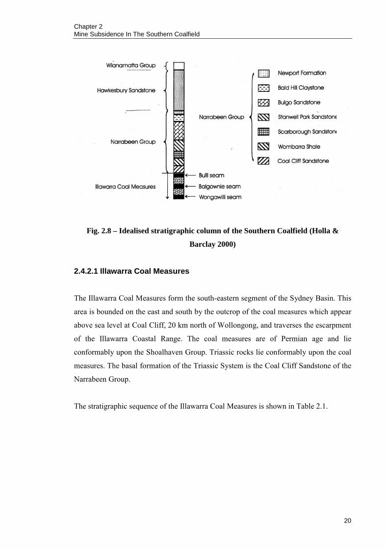
Fig. 2.8 – Idealised stratigraphic column of the Southern Coalfield (Holla &
Barclay 2000)
2.4.2.1 Illawarra Coal Measures
The Illawarra Coal Measures form the south-eastern segment of the Sydney Basin. This
area is bounded on the east and south by the outcrop of the coal measures which appear
above sea level at Coal Cliff, 20 km north of Wollongong, and traverses the escarpment
of the Illawarra Coastal Range. The coal measures are of Permian age and lie
conformably upon the Shoalhaven Group. Triassic rocks lie conformably upon the coal
measures. The basal formation of the Triassic System is the Coal Cliff Sandstone of the
Narrabeen Group.
The stratigraphic sequence of the Illawarra Coal Measures is shown in Table 2.1.
Chapter 2 Mine Subsidence In The Southern Coalfield
21
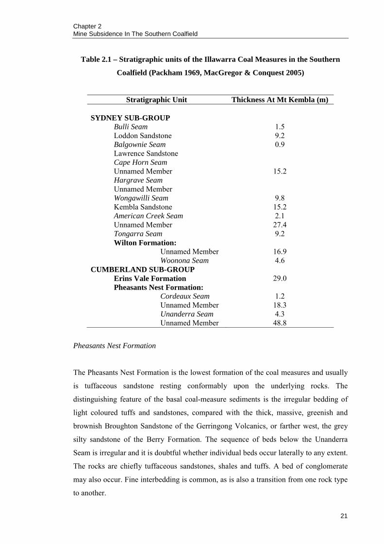
Table 2.1 – Stratigraphic units of the Illawarra Coal Measures in the Southern
Coalfield (Packham 1969, MacGregor & Conquest 2005)
Stratigraphic Unit Thickness At Mt Kembla (m)
SYDNEY SUB-GROUP Bulli Seam 1.5 Loddon Sandstone 9.2 Balgownie Seam 0.9 Lawrence Sandstone Cape Horn Seam Unnamed Member 15.2 Hargrave Seam Unnamed Member Wongawilli Seam 9.8 Kembla Sandstone 15.2 American Creek Seam 2.1 Unnamed Member 27.4 Tongarra Seam 9.2 Wilton Formation:
Unnamed Member 16.9 Woonona Seam 4.6
CUMBERLAND SUB-GROUP Erins Vale Formation 29.0 Pheasants Nest Formation:
Cordeaux Seam 1.2 Unnamed Member 18.3 Unanderra Seam 4.3 Unnamed Member 48.8
Pheasants Nest Formation
The Pheasants Nest Formation is the lowest formation of the coal measures and usually
is tuffaceous sandstone resting conformably upon the underlying rocks. The
distinguishing feature of the basal coal-measure sediments is the irregular bedding of
light coloured tuffs and sandstones, compared with the thick, massive, greenish and
brownish Broughton Sandstone of the Gerringong Volcanics, or farther west, the grey
silty sandstone of the Berry Formation. The sequence of beds below the Unanderra
Seam is irregular and it is doubtful whether individual beds occur laterally to any extent.
The rocks are chiefly tuffaceous sandstones, shales and tuffs. A bed of conglomerate
may also occur. Fine interbedding is common, as is also a transition from one rock type
to another.
Chapter 2 Mine Subsidence In The Southern Coalfield
22
Thin intermittent coal seams have been observed within the sequence of the Pheasants
Nest Formation. The Unanderra Seam is the lowest named seam in the coal measures. It
is known in the Mt Kembla – Mt Keira area where is occurs about 45 m above the base
of the coal measures. It consists predominately of carbonaceous shale with thin plies of
coal.
The sequence above the Unanderra Seam consists of irregularly interbedded tuffaceous
sandstones, shales and tuffs. Individually the beds are thin and insignificant. Knowledge
of these beds is also confined to the Mt Kembla area. A minor coal seam, up to 10 cm
thick, occurs in this sequence. The Cordeaux Seam is a thin seam of carbonaceous and
tuffaceous shale containing coal bands. It is only known in the Mt Kembla – Mt Nebo
area. Its thickness is variable up to a maximum of 1.2 m. The maximum recorded
thickness of the Pheasants Nest Formation is 120 m (Packham 1969).
Erins Vale Formation
This formation apparently marks the commencement of a more stable depositional
environment. Bedding becomes more regular and the sediments are not so distinctly
tuffaceous. Calcite, although present, does not occur so prominently as veins and
facings as in the lower sediments. Nevertheless, individual beds are not persistent. The
rocks in the sequence are tuffaceous sandstones, which predominate, and shales. Gritty
and conglomeratic sandstones appear occasionally, especially in the upper part of the
formation. The maximum recorded thickness of the formation is 120 m (Packham
1969).
Wilton Formation
The Woonona Seam, the basal member of the Wilton Formation and of the Sydney Sub-
Group, is much more persistent than any of the lower seams. It outcrops above sea level
at Thirroul in the north and extends to about Macquarie Pass in the south. It has not
been found on the southern edge of the coalfield. The seam is up to 6 m thick and is
subject to splitting in some areas. It consists of coal and shaly coal and usually, although
not always, contains numerous bands of shale. The most economic development of the
seam is in the Mt Kembla area where it is 4.6 m thick, with a workable section 2.5 m
Chapter 2 Mine Subsidence In The Southern Coalfield
23
thick, which contains 24 % ash, excluding shale bands. The seam, however, is not
worked at the moment. The coal has weak coking properties.
The interval between the Woonona Seam and the Tongarra Seam consists of beds of
shales and sandstones which, although distinct in local areas, do not persist laterally.
Generally sandstone is the subordinate rock type. The thickness of the strata varies
between 15 m and 75 m (Packham 1969).
Tongarra Seam
The Tongarra Seam is subject to splitting by a bed of sandstone in some areas. Usually
the seam consists of coal of variable quality and shale bands. It apparently occurs
throughout most of the coalfield but less is known of its characteristics in the western
half of the field. It is the lowest seam occurring on the southern edge of the field.
Thickness varies from 1.2 m to 6.7 m. Its best development is in the Tongarra and
Avondale areas where parts of the seam are of quality suitable for mining. Here the
worked section, excluding shale bands, contains approximately 20 % ash. The coal has
medium coking properties.
The interval between the Tongarra and American Creek Seams consist essentially of
dark grey shale containing minor beds of sandstone. A significant bed of yellowish
white tuffaceous shale of 30 cm average thickness occurs about 4.6 m above the
Tongarra Seam. It has not been identified over the whole field but where it can be
recognised it serves as a valuable marker horizon. The sediments vary in thickness
between 9 m and 30 m (Packham 1969).
American Creek Seam
The American Creek Seam consists chiefly of carbonaceous shale and coal. In the past,
the seam has been worked as a source of oil shale in the Mt Kembla area. The seam
varies in thickness and character, lateral variation in places being sudden. Although it
occurs throughout the whole field its development is discontinuous, presumably owing
to local washouts or areas of non-deposition. Its thickness ranges usually up to a
maximum of 7.5 m (Packham 1969).
Chapter 2 Mine Subsidence In The Southern Coalfield
24
Kembla Sandstone
The Kembla Sandstone is usually a massive, light-grey, medium-grained sandstone,
occasionally coarse or with conglomeratic phases, which grades vertically upwards
through a sandy shale to a carbonaceous shale immediately below the Wongawilli
Seam. In places a basal shale member may also exist. The thickness of the Kembla
Sandstone varies between 4.5 m and 15 m (Packham 1969).
Wongawilli Seam
The Wongawilli Seam extends over the whole coalfield. Its thickness ranges from 6 m
in the south to 15 m in the northeast. Over most of the field, however, a range of 9 m to
11 m is maintained. The seam consists of coal plies of varying quality, separated by
bands or beds of shale, mostly carbonaceous or coal or tuffaceous. One bed, which is a
hard, sandy, cream-coloured tuff, known colloquially as the Sandstone Band,
characterises the seam. Over part of the field the lowest 1.8 m to 3.7 m of the seam
contains coal of commercial quality. In collieries where the seam is mined, the worked
section contains 20 % to 30 % ash. The coal plies, that is, excluding shale bands,
contain 15 % to 25 % ash and have strong coking properties. In some localities a system
of sills intrudes the seam over wide areas.
The interval between the Wongawilli Seam and the Balgownie Seam consists of shale,
sandstone and one or two minor coal seams. In the northern coastal area the two minor
coal seams are known as the Cape Horn and Hargrave Seam and divide the sequence as
shown in Table 2.2.

Chapter 2 Mine Subsidence In The Southern Coalfield
25
Table 2.2 – Interval between Wongawilli and Balgownie Seams (Packham 1969)
Stratigraphic Unit Thickness (m)
Balgownie Seam Lawrence Sandstone: Medium-grained massive sandstone overlain by shale
11
Cape Horn Seam 1.2 Dark-grey shale containing sandstone beds 3.0 Hargrave Seam 0.3 Interbedded sandstone and shale 7.0 Wongawilli Seam
The thicknesses quoted are for the Scarborough area. The total thickness is 23 m
compared with 27 m in the Helensburgh area to the north where the Lawrence
Sandstone remains constant in thickness while the other sediments thicken. South and
west of this area the coal seams become less definite although in any particular locality,
except perhaps in the far south, some coal is always present.
In the central part of the field, a thin coal seam of 30 cm average thickness is overlain
by sandstone and underlain by shale. The seam extends over a wide area and may prove
to be the extension of the Cape Horn Seam. The overlying sandstone, which is about 6
m thick, may thus correspond to the Lawrence Sandstone. In the central and southern
parts of the field the interval between the Wongawilli and Balgownie Seams is reduced
to 15 m and less (Packham 1969).
Balgownie Seam
The Balgownie Seam exceeds 1.5 m in thickness in the extreme north eastern part of the
field but shows a steady decrease in thickness to the south and west. South of
Macquarie Pass it is less than 30 cm thick, although generally it is of good quality. It
usually consists of un-banded clean coal and contains about 15 % ash. The coal is of
medium coking quality. Commercially the Balgownie Seam is attractive from the aspect
of coal quality but unattractive from the aspect of thickness.
Like the Balgownie Seam, the formation between it and the Bulli Seam decreases in
thickness from the northeast to the west and south. Its thickness averages 9 m varying
Chapter 2 Mine Subsidence In The Southern Coalfield
26
between 4.5 m to 15 m. The formation consists essentially of light-grey, medium-
grained massive sandstone called the Loddon Sandstone. This is invariably overlain by
a bed of dark-grey shale, usually less than 3 m thick, which at the top becomes
carbonaceous to form the floor of the Bulli Seam (Packham 1969).
Bulli Seam
The Bulli Seam is the topmost formation in the Illawarra Coal Measures. Commercially
it is the most important of the coal seams and has been extensively mined. Thickness of
the seam is a maximum of 4 m in the northern part of the field with a regional decrease
to the south. In the vicinity of Mt Kembla such decrease becomes rapid and farther
south of this point the seam is represented by about 60 cm of coal and shale. In the far
south the seam is less than 30 cm thick and consists chiefly of carbonaceous shale. In
the extreme southwest part of the field the seam is absent, and owing to
contemporaneous erosion, the section overlying the Wongawilli Seam has been replaced
by Triassic rocks. North of its rapid thickness change near Mt Kembla the seam is over
1.5 m thick.
In its areas of best development, that is, north of Mt Kembla, the Bulli Seam consists
essentially of clean coal containing in places thin shale bands. Its ash content is
remarkably consistent, only rising above the general range of 9 % to 12 % at the
northern end of the field. Its coking properties vary generally from medium to strong
but are weak in one or two localities. The Bulli Seam is overlain by the Coal Cliff
Sandstone of the Narrabeen Group (Packham 1969).
2.4.2.2 Narrabeen Group
The Narrabeen Group is known to occur throughout the Sydney Basin. It extends along
the Illawarra coastal escarpment and also outcrops to the west of the escarpment. This
group includes the main sequence of rocks along the coastal cliffs between Stanwell
Park and Scarborough, where it is particularly well exposed. The lowest units of the
Narrabeen Group are Late Permian and the upper unit is Middle to Late Triassic in age.
The thickness of the Narrabeen Group decreases to the south.

Chapter 2 Mine Subsidence In The Southern Coalfield
27
The Narrabeen Group includes the Coal Cliff Sandstone, Wombarra Shale, Otford
Sandstone Member, Scarborough Sandstone, Stanwell Park Claystone, Bulgo
Sandstone, Bald Hill Claystone, Garie Formation and the Newport Formation. The
Hawkesbury Sandstone overlies the Narrabeen Group (Ghobadi 1994).
Coal Cliff Sandstone
The Coal Cliff Sandstone is the basal unit of the Narrabeen Group and overlies the
Illawarra Coal Measures. The thickness of the unit ranges between 6 m and 20 m
(Hanlon 1953). The Coal Cliff Sandstone is a light grey, fine to medium grained,
quartz-lithic and lithic sandstone with a number of pebble and shale bands. It crops out
in the coastal section near Clifton and passes below sea level north of Coalcliff. Angular
siderite fragments up to 10 cm in size are common in the basal Coal Cliff Sandstone.
This unit forms the roof of some colliery workings and is exposed underground for
several kilometres to the west of the Illawarra escarpment. In some places colliery roofs
are less stable because the fine sandstone near the base of the Coal Cliff Sandstone
sometimes grades into shale (Ghobadi 1994).
Wombarra Shale
The Coal Cliff Sandstone is overlain by 6 m to 30 m of greenish-grey shale with lithic
sandstone interbeds. It is well exposed in road cuttings and cliffs south of Coalcliff. The
sandstone interbeds are generally quite thin, lenticular, fine-grained and carbonate-
cemented. Towards the top of the formation, a thicker sandstone unit is called the
Otford Sandstone Member (Ghobadi 1994).
Scarborough Sandstone
The Scarborough Sandstone overlies the Wombarra Shale. Commonly the Scarborough
Sandstone is conglomeratic with coloured chert clasts especially in the basal half. It
consists of beds up to several metres in thickness which becomes finer upwards. This
unit comprises lithic to quartz-lithic sandstone with pebbles and minor amounts of grey
shale (Ghobadi 1994).

Chapter 2 Mine Subsidence In The Southern Coalfield
28
Stanwell Park Claystone
This unit overlies the Scarborough Sandstone. It consists of interbedded green to
chocolate shale and sandstone. Three claystone intervals and two sandstone beds can be
recognized. The lower section of the unit consists of greenish-grey claystone and
sandstone which slowly changes upward into red-brown claystone and clay. The
sandstone beds are composed of weathered lithic fragments and are usually light
greenish-grey in colour. The relative proportion of claystone and sandstone varies but
overall they are sub-equal (Bowman 1974).
Bulgo Sandstone
The Bulgo Sandstone, which rests on the Stanwell Park Claystone, is the thickest unit of
the Narrabeen Group on the Illawarra coast. It forms prominent outcrops in the area and
between Coalcliff and Clifton. It consists of thickly bedded sandstone with intercalated
siltstone and claystone beds up to 3 m thick. Conglomerate is also present, especially
toward the base. The Bulgo Sandstone has a higher proportion of quartz than of rock
fragments. Sandstone beds rarely exceed 4 m in thickness while the siltstone and shale
interbeds are usually less than 1 m thick (Ghobadi 1994).
Bald Hill Claystone
The Bald Hill Claystone, which overlies the Bulgo Sandstone, outcrops in the hills near
Otford and on the Mt Ousley road to the south. This formation is about 15 m thick in the
Bald Hill area (Hanlon 1953). It consists almost entirely of claystone, but lithic
sandstone interbeds are found towards the base of the unit. Mottled chocolate and green
claystone zones are common (Ghobadi 1994).
Garie Formation
Toward the top of the Bald Hill Claystone, thin beds of light coloured claystone become
more common. This upper zone passes into a mid-grey slightly carbonaceous massive
claystone, which is overlain in turn, by the Newport Formation. The Garie Formation is

Chapter 2 Mine Subsidence In The Southern Coalfield
29
usually less than 3 m thick but it is a very good marker horizon in the southern Sydney
Basin (Ghobadi 1994).
Newport Formation
The mid-grey shale and minor interbedded lithic sandstone of the Newport Formation
overlies the Garie Formation. Mud-rocks of this formation are thinly bedded. The dark-
grey mud-rocks contain plentiful plant fossils. Claystone beds consisting of sand-sized
flakes of kaolinite, with a large original porosity, are common in the Newport
Formation (Bowman 1974).
2.4.2.3 Hawkesbury Sandstone
This unit is flat-lying Middle Triassic quartz sandstone that crops out at the top of most
the Illawarra escarpment. It forms a resistant plateau to the west of the escarpment,
which gently dips to the northwest. The formation has a thickness of about 180 m at
Stanwell Park. It contains a minor amount of mudstone, interbedded with fine
sandstone, but it consists dominantly of sandstone beds (Jones & Rust 1983) typically
2 m to 5 m but up to 15 m in thickness. Transition into conglomerate is seen in some of
the sandstone beds. Strong cross-bedding is common in the Hawkesbury Sandstone. The
interbedded mudstone is very prone to weathering upon exposure and the Hawkesbury
Sandstone is often involved in rock falls from the escarpment.
2.5 CURRENT PREDICTION TECHNIQUES USED IN THE SOUTHERN COALFIELD
Empirical a. based on observation or experiment, not on theory.
Empirical prediction methods provide an instrument in which reasonably accurate
subsidence predictions can be made, provided the user is aware of the limitations of
such methods. Subsidence prediction in the Southern Coalfield by empirical methods is
mainly limited to the guidelines proposed by Holla and Barclay (2000), published by
the New South Wales Department of Primary Industries (formerly the New South
Wales Department of Mineral Resources), and the Incremental Profile Method
Chapter 2 Mine Subsidence In The Southern Coalfield
30
(Waddington & Kay 1995) that was developed by Mine Subsidence Engineering
Consultants (formerly Waddington Kay and Associates). The Incremental Profile
Method attempts to address the shortfalls of the New South Wales Department of
Primary Industries empirical method, mainly in the areas of multiple longwall panel
subsidence and longwall mining effects on river valleys. This section will cover both
empirical methods.
2.5.1 New South Wales Department of Primary Industries Empirical Technique
The method devised by the New South Wales Department of Primary Industries has
been in existence since the mid 1980’s (Holla 1985). Since then, the method has been
refined with the addition of subsidence data (up to June 2000), and a discussion on the
effects of mining induced subsidence on public utilities, dwellings and water bodies.
Whilst not accounted for in the prediction technique, there is also a discussion on the
major factors modifying the theoretical subsidence behaviour such as faults, dykes, and
gullies. Several case studies are also presented to illustrate these factors in action.
2.5.1.1 Overview of method
The subsidence data and resulting graphs in this method were obtained from collieries
in the area between the Illawarra Escarpment and the Burragorang Valley. This data was
collected over a period of thirty years. The majority of the mines included in the
analyses were mining the Bulli seam except in two cases for which the workings were
in the Wongawilli seam. The predominant method of mining was by longwall mining,
although some pillar extraction data has been included.
The basic inputs that are required for this method are:
Width of longwall panel (W),
Depth of cover (H),
Mined seam height (T), and
Pillar width (Pw) (multiple longwall panel layouts).

Chapter 2 Mine Subsidence In The Southern Coalfield
31
Once these parameters are known, it is possible to predict the following parameters for a
given single longwall panel mining layout:
Maximum developed subsidence (Smax),
Maximum tensile strain (+Emax),
Maximum compressive strain (-Emax),
Maximum ground tilt (Gmax),
Radius of ground curvature (Rmin),
Location of inflection point, and
Goaf edge subsidence (Sgoaf).
With these parameters it is possible to produce a subsidence profile as shown in
Figure 2.9. It must be noted that only the maximum developed subsidence can be
predicted for multiple longwall panels.
Fig. 2.9 – Formation of a subsidence trough above an extraction panel (Holla &
Barclay 2000)

Chapter 2 Mine Subsidence In The Southern Coalfield
32
2.5.1.2 Maximum developed subsidence for single longwall panels
Maximum developed subsidence is a function of the longwall panel width to depth of
cover ratio (W/H) and the extracted thickness (T). Generally, the larger the W/H ratio,
the greater the subsidence. If a longwall panel is fixed at a depth of 400 m and is 200 m
wide, it would generally produce greater subsidence than if the same longwall panel was
150 m wide. This is mainly due to the bridging capability of the strata above the
extracted longwall panel.
Figure 2.10 is used for predicting the maximum developed subsidence over a single
longwall panel. It can be seen in Figure 2.10 that the subsidence factor (Smax/T)
increases substantially for W/H ratios greater than 0.5. This would suggest that
subsidence is no longer controlled by the elastic deformation/sag of the strata and that
the bridging capability of the strata is reached at this value.
Fig. 2.10 – Relationship between W/H ratio and Smax/T for single panels (Holla &
Barclay 2000)
It can be seen from Figure 2.10 that the largest longwall W/H ratio still falls into the
sub-critical category (W/H < 1.4). This is a result of the deep mining conditions in the
Southern Coalfield, and although data exists for W/H ratios between 0.5 and 0.9, the

Chapter 2 Mine Subsidence In The Southern Coalfield
33
resulting scatter suggests that subsidence prediction would be more accurate for W/H
ratios less than 0.5.
Another point to note, and which has been addressed by Holla and Barclay (2000), is
that Figure 2.10 suggests that the maximum developed subsidence from pillar extraction
is greater than that for longwall extraction. One reason given argues that for longwall
extraction, unmined coal is concentrated in chain pillars and for pillar extraction;
unmined coal is spread out over the goaf area in the form of stooks. The reason for the
greater developed subsidence from pillar extraction is simply that chain pillars, by their
dimensions, are inherently stronger than smaller stooks. Another reason that is raised is
the validity of the pillar extraction data. It is pointed out that in some cases, old
workings next to new pillar extraction panels may have influenced the quality of the
data set, and in many cases was difficult to identify.
2.5.1.3 Maximum developed subsidence for multiple longwall panels
More often than not, the need to predict the subsidence produced by one single isolated
longwall panel in virgin coal is not that great. In practise, it is not uncommon for a
series of ten or more longwall panels to be mined. These longwall panels are separated
by chain pillars and it has been observed by Holla and Barclay (2000) that the
subsidence over multiple longwall panel layouts is controlled primarily by the
compression of pillar coal and strata located both above and below the seam. Longwall
panels in the Southern Coalfield are generally narrow enough to allow the strata to
bridge between the pillars, reducing the sag component of subsidence while increasing
pillar compression.
It can be seen from Figure 2.11, and noted by Holla and Barclay (2000), that the
maximum subsidence does not develop until four to five longwall panels have been
mined for a particular geometry. This is a result of the incremental loading of pillars as
mining progresses, up to a point where the pillar stress reaches a maximum (in this case
after four to five longwall panels). At this stage, the differences in the maximum
subsidence for different layouts are due to differences in pillar loads and stresses,
therefore implying that pillar deformation is the significant contributor to the maximum
developed subsidence. Recently, this characteristic has been noted by Mills and

Chapter 2 Mine Subsidence In The Southern Coalfield
34
Huuskes (2004) at Metropolitan Colliery, where the overall magnitude of subsidence is
controlled by the elastic compression of the chain pillars and the strata above and below
the chain pillars. It was proposed that subsidence occurs in response to the ‘super-panel’
effect of multiple longwall panels, rather than in response to individual longwall panels.
Figure 2.11 and Figure 2.12 are used to predict the subsidence for multiple longwall
panel layouts.
Fig. 2.11 – Relationship between W/H and Smax/T for multiple panels (Holla &
Barclay 2000)
Given the important role that chain pillars play in subsidence development, a
relationship was established between the loading on the pillar and the subsidence factor
(Smax/T). This can be seen in Figure 2.12.
The area of overburden loading a pillar in a multiple longwall panel layout is given by
Equation 2.5:
⎟⎟⎠
⎞⎜⎜⎝
⎛⎟⎠⎞
⎜⎝⎛Φ×−=
4tan2WHWArea L [2.5]

Chapter 2 Mine Subsidence In The Southern Coalfield
35
Where,
WL = Longwall panel width + pillar width (m)
H = Depth of cover (m)
Φ = Abutment angle (°)
For mines operating in the Bulli Seam where H is greater than 350 m, it is
recommended that 21˚ should be used for the abutment angle (Colwell Geotechnical
Services 1998).
However, for this value of the abutment angle the second term ((W)2 x tan(Φ/4)) is
small compared to the first term (WLH). Therefore, pillar load can be taken as a function
of (WLH) and the pillar stress (WLH/PW).
Fig. 2.12 – Relationship between pillar stress factor (WLH/Pw) and Smax/T for
multiple panel layouts (Holla & Barclay 2000)
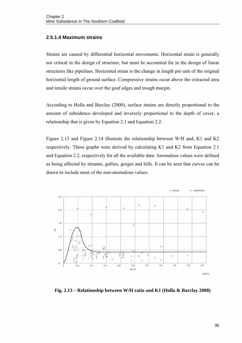
Chapter 2 Mine Subsidence In The Southern Coalfield
36
2.5.1.4 Maximum strains
Strains are caused by differential horizontal movements. Horizontal strain is generally
not critical in the design of structure, but must be accounted for in the design of linear
structures like pipelines. Horizontal strain is the change in length per unit of the original
horizontal length of ground surface. Compressive strains occur above the extracted area
and tensile strains occur over the goaf edges and trough margin.
According to Holla and Barclay (2000), surface strains are directly proportional to the
amount of subsidence developed and inversely proportional to the depth of cover, a
relationship that is given by Equation 2.1 and Equation 2.2.
Figure 2.13 and Figure 2.14 illustrate the relationship between W/H and, K1 and K2
respectively. These graphs were derived by calculating K1 and K2 from Equation 2.1
and Equation 2.2, respectively for all the available data. Anomalous values were defined
as being affected by streams, gullies, gorges and hills. It can be seen that curves can be
drawn to include most of the non-anomalous values.
Fig. 2.13 – Relationship between W/H ratio and K1 (Holla & Barclay 2000)
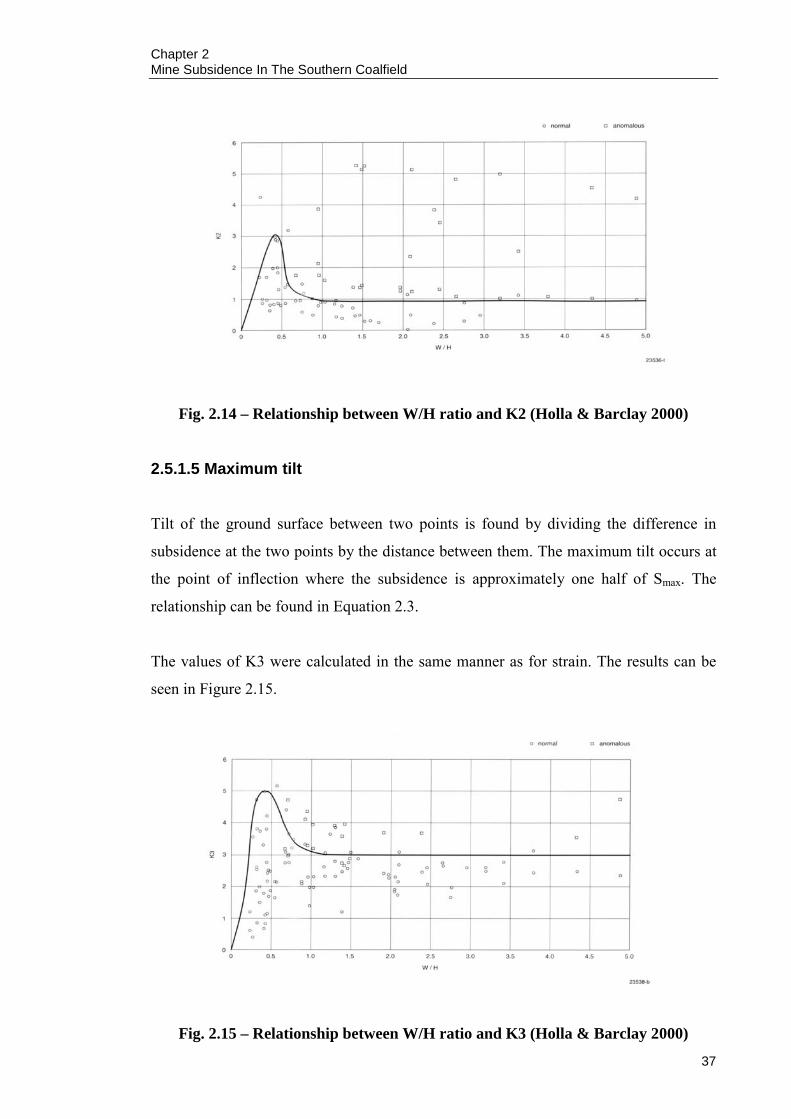
Chapter 2 Mine Subsidence In The Southern Coalfield
37
Fig. 2.14 – Relationship between W/H ratio and K2 (Holla & Barclay 2000)
2.5.1.5 Maximum tilt
Tilt of the ground surface between two points is found by dividing the difference in
subsidence at the two points by the distance between them. The maximum tilt occurs at
the point of inflection where the subsidence is approximately one half of Smax. The
relationship can be found in Equation 2.3.
The values of K3 were calculated in the same manner as for strain. The results can be
seen in Figure 2.15.
Fig. 2.15 – Relationship between W/H ratio and K3 (Holla & Barclay 2000)
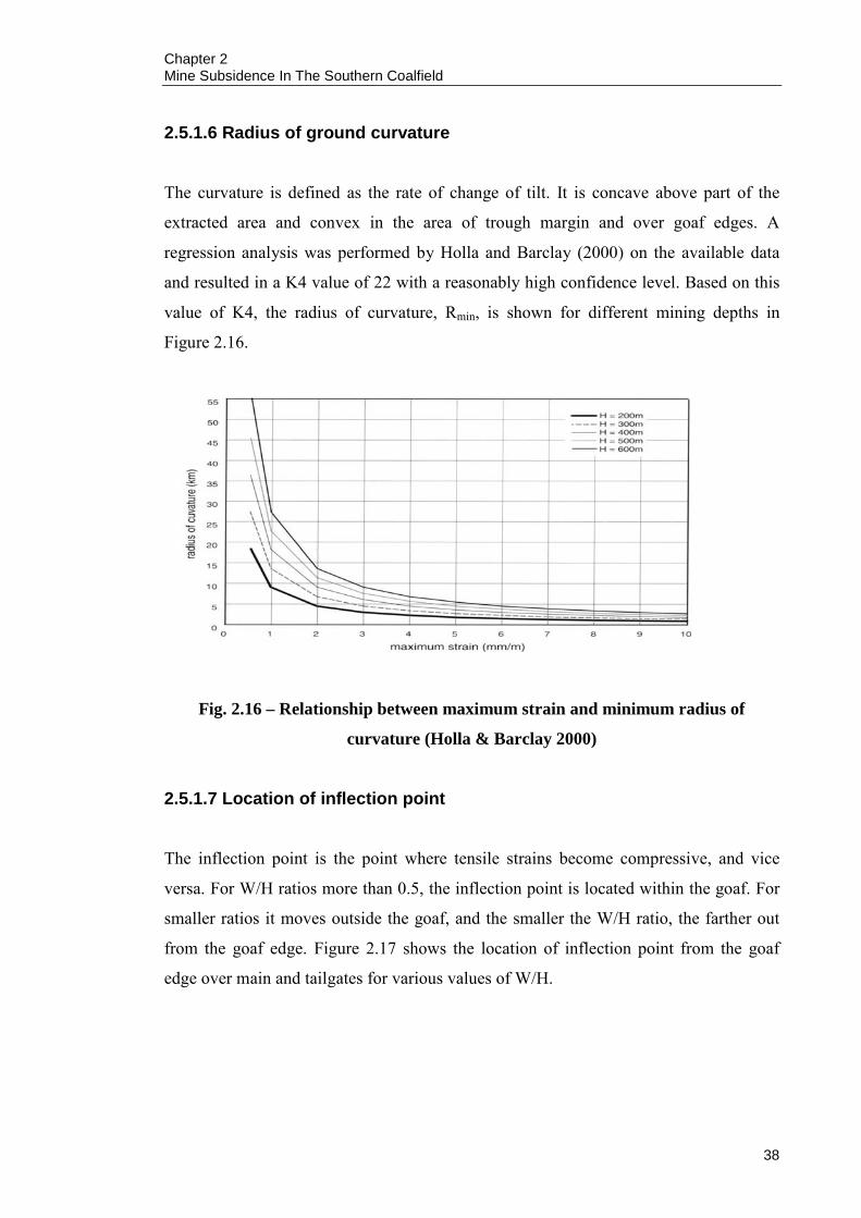
Chapter 2 Mine Subsidence In The Southern Coalfield
38
2.5.1.6 Radius of ground curvature
The curvature is defined as the rate of change of tilt. It is concave above part of the
extracted area and convex in the area of trough margin and over goaf edges. A
regression analysis was performed by Holla and Barclay (2000) on the available data
and resulted in a K4 value of 22 with a reasonably high confidence level. Based on this
value of K4, the radius of curvature, Rmin, is shown for different mining depths in
Figure 2.16.
Fig. 2.16 – Relationship between maximum strain and minimum radius of
curvature (Holla & Barclay 2000)
2.5.1.7 Location of inflection point
The inflection point is the point where tensile strains become compressive, and vice
versa. For W/H ratios more than 0.5, the inflection point is located within the goaf. For
smaller ratios it moves outside the goaf, and the smaller the W/H ratio, the farther out
from the goaf edge. Figure 2.17 shows the location of inflection point from the goaf
edge over main and tailgates for various values of W/H.

Chapter 2 Mine Subsidence In The Southern Coalfield
39
Fig. 2.17 – Location of inflection point (Holla & Barclay 2000)
2.5.1.8 Goaf edge subsidence
Goaf edge subsidence values for various W/H ratios can be seen in Figure 2.18. It is
noted that for subcritical longwall panels, the goaf edge subsidence forms much of the
maximum developed subsidence.
Fig. 2.18 – Goaf edge subsidence (Holla & Barclay 2000)

Chapter 2 Mine Subsidence In The Southern Coalfield
40
2.5.2 The Incremental Profile Method
The Incremental Profile Method was developed by MSEC (formerly Waddington Kay
and Associates) in 1994 during the course of a study for BHP Collieries Division, the
Water Board and AGL (Waddington Kay and Associates 2002). The purpose of the
study was to develop an empirical model that could predict subsidence, tilts, curvatures,
strains and surface effects as a result of longwall mining at Appin and Tower Collieries.
2.5.2.1 Overview of method
Historical subsidence data from Appin, Tower, Tahmoor, West Cliff, Cordeaux and
South Bulli Collieries was studied and plotted in a variety of ways in order to identify a
regular pattern of ground behaviour. The most significant patterns were found in the
shapes of the incremental subsidence profiles measured along survey lines transversely
across the longwall panels.
The incremental subsidence profile for each longwall panel was derived by subtracting
the initial subsidence profile measured before mining the longwall panel, from the final
subsidence profile measured after mining the longwall panel. The incremental
subsidence profile for a longwall panel shows the change in the subsidence profile
caused by the mining of the longwall panel.
Figure 2.19 is an illustration of typical incremental subsidence profiles.

Chapter 2 Mine Subsidence In The Southern Coalfield
41
Fig. 2.19 – Typical incremental subsidence profiles, NSW Southern Coalfield
(Waddington Kay & Associates 2002)
The Incremental Profile Method is based on predicting the incremental subsidence
profile for each longwall panel in a series of longwall panels and then adding the
respective incremental profiles to show the cumulative subsidence profile at any stage in
the development of a series of longwall panels. Incremental tilts, curvatures and strains
can also be predicted. Profiles in both the transverse and longitudinal directions can be
predicted, thereby allowing predictions to be made on any point on the surface above a
series of longwall panels.
Initially designed for the Southern Coalfield, the method has been applied to the
Newcastle Coalfield and used to predict subsidence at West Wallsend, Cooranbong,
Wyong and South Bulga Collieries. Further research by the authors of this method has
involved the potential application of the Incremental Profile Method in multi-seam
situations. It was found that the multi-seam profiles are generally greater in amplitude
than single seam profiles and differ in shape from the standard profile over single
seams.

Chapter 2 Mine Subsidence In The Southern Coalfield
42
The incremental profiles have been modelled in two halves, the point of maximum
subsidence being the point at which the two halves of the profile meet. A library of
mathematically defined profile shapes has been established, which allows the
incremental profiles to be modelled, depending on the width to depth ratio of the
longwall and the position of the longwall panel in the series. The mathematical
formulae that define the profile shape are of the form given in Equation 2.6. The library
of profile shapes comprise the values of a to k in these formulae.
5432
5432
1 jxhxfxdxbxkxixgxexcxay
++++++++++= [2.6]
Different formulae apply, with unique a to k values, for first, second, third, fourth, and
fifth or subsequent longwall panels in a series, and for different width to depth ratios,
within the range of 0.3 to 5.0. For second, third, fourth and fifth or subsequent longwall
panels, the left and right hand side of the profiles have different formulae.
The library of profile shapes contains a to k values for 693 different half-profile shapes
for single-seam mining operations. The library also contains 236 different half-profile
shapes for a range of multi-seam mining situations. A selection of model incremental
subsidence profiles for various width to depth ratios is shown in Figure 2.20.
It has been acknowledged by the authors that the method has a tendency to over-predict
the subsidence parameters as a conservative view was adopted in drafting the graph
(Figure 2.21) that is used for predicting the maximum incremental subsidence. Figure
2.21 shows the maximum incremental subsidence, expressed as a proportion of seam
thickness, versus longwall panel width to depth ratio.
Since Figure 2.21 is used to determine the amplitude of the incremental subsidence
profile, any over-prediction of the maximum subsidence value also leads to over-
predictions of the tilt, curvature and strain values. Once the geometry of a longwall
panel is known, the shapes of the two halves of the incremental subsidence profile of
the longwall panel can be determined from the appropriate formulae to provide a
smooth non-dimensional subsidence profile across the longwall panel.

Chapter 2 Mine Subsidence In The Southern Coalfield
43
Fig. 2.20 – Incremental subsidence profiles obtained using the Incremental Profile
Method (Waddington Kay & Associates 2002)
Fig. 2.21 – Prediction curves for maximum incremental subsidence (Waddington
Kay & Associates 2002)
Chapter 2 Mine Subsidence In The Southern Coalfield
44
The actual incremental profile is obtained by multiplying vertical dimensions by the
maximum incremental subsidence value and horizontal dimensions by the local depth of
cover. Smooth tilt and curvature profiles are obtained by taking the first and second
derivatives of the subsidence profile.
The amplitude and position of the incremental profile relative to the advancing goaf
edge of the longwall is determined by a factor known as the overlap factor, the profile
moving further towards the previous longwall panel as the overlap factor increases. This
factor is an empirically derived factor, which is a function of the longwall panel width,
pillar width and the depth of cover.
In order to determine strain values from the curvature graphs, it is necessary to select an
empirical relationship that will generally provide conservative results. The NCB
Subsidence Engineers’ Handbook (National Coal Board 1975) adopts a relationship in
which the reciprocal radius of curvature, K, is equal to strain squared divided by 0.024.
The authors state this relationship does not provide a good fit when predicted strains,
derived from predicted curvatures are compared with measured values, and a better fit is
obtained if a linear relationship of strain = 15 x curvature is chosen, which equates to
the bending strain in a beam of 30 m depth bending about its centre line.
The authors point out that the relationship of 15 times curvature is also reasonably close
to the graph of radius of curvature versus maximum strain (Figure 2.16) for depths of
cover between 300 m and 400 m. It has been found that a multiplying factor of 10 gives
better results in the Newcastle Coalfield.
Predicted horizontal displacements in the direction of the prediction line can be derived
by accumulating the predicted strains multiplied by the bay lengths, after distributing
any displacement closure errors over all bay lengths in proportion to the predicted
strains. Alternatively, the predicted horizontal ground movement profiles can be derived
by applying a proportionality factor to the predicted tilt profiles, which they resemble in
both magnitude and direction. If the latter method is adopted, it is stated that it should
be realised that the actual shapes of the horizontal displacement profile and the tilt
profile are different and that the predicted horizontal movements at low tilt values could
be understated.

Chapter 2 Mine Subsidence In The Southern Coalfield
45
The authors state that the predicted subsidence and tilt profiles obtained using the
Incremental Profile Method usually match the observed profiles reasonably accurately,
and it is not possible to match the predicted and observed curvature and strain profiles
to the same standard, due to the large amount of scatter in the measured data, although
the range of strains are adequately predicted.
2.6 SUMMARY
In this chapter, subsidence theory was reviewed and particular attention was paid to the
caving characteristics of the Southern Coalfield. The caving characteristics have been
identified as one of the distinguishing features in terms of numerical model validation.
The empirical methods of Holla and Barclay (2000) and Waddington and Kay (2002)
were also reviewed and the following is a summary of the advantages and disadvantages
regarding the empirical methods.
DPI Empirical Method Advantages
Easy to use,
Reasonably accurate for W/H < 0.5 (a variation of 10 % should be accounted
for),
Predictions can be made in a relatively short time (when compared to other
methods such as numerical modelling, influence and profile functions), and
A complete subsidence profile can be obtained for a single longwall panel
extraction.
DPI Empirical Method Disadvantages
Only applicable to longwall mining,
Large scatter in data evident in Figures 2.10, 2.13, 2.14, 2.15, 2.17 and 2.18
(Smax/T for single longwall panels, K1, K2, K3, inflection point and goaf edge
subsidence respectively),
Predicted limit of mining influence affected by the determination of the draw
angle (large variation in observed values) and the uncertain extent of horizontal
movement,

Chapter 2 Mine Subsidence In The Southern Coalfield
46
Cannot produce a subsidence profile for multiple longwall panel layouts,
Cannot predict subsidence in topography that is not relatively flat,
Cannot predict subsidence for multiple seam mining,
Cannot predict location and depth of surface cracking due to the acknowledged
difficulty in predicting surface strains, and
Cannot predict sub-surface deformations – must rely on assumptions.
Incremental Profile Method Advantages
Multiple longwall panel application,
Multiple seam application,
Can predict transverse and longitudinal profiles anywhere above a series of
longwall panels,
Can predict horizontal displacements,
Allows for variation in seam thickness, pillar and longwall panel widths, and
depths of cover across a series of longwall panels, and
Applicable to other coalfields (e.g. Newcastle Coalfield).
Incremental Profile Method Disadvantages
Only applicable to longwall mining,
Large data scatter problematic for localised strain predictions, and
Not as simple to use compared to DPI method.

Chapter 3 Valley Closure And Upsidence
47
CHAPTER 3 VALLEY CLOSURE AND UPSIDENCE
3.1 INTRODUCTION
Valley closure and upsidence are phenomena that occur when mining approaches and
undermines river valleys. The most common effects of valley closure and upsidence are
cracking and buckling of river beds and rock bars, localised loss of water flow and
adverse effects on the local ecosystem (Figures 3.1 to 3.3). In most cases, the loss of
water flow into voids beneath the base of the valley is caused by the cracking and
buckling of the valley base. The magnitude of water loss is dependant on the gradient of
the creek/river, relative water table levels and the magnitude of the water flows. Where
losses occur it is generally temporary and this water re-joins the creek/river further
downstream (Waddington & Kay 2001). The most common method of rehabilitation
involves the injection of some type of grout to try and seal the mining induced rock
fracture network and restore water flow.
Fig. 3.1 – Buckling of rock bars resulting in low angle fractures
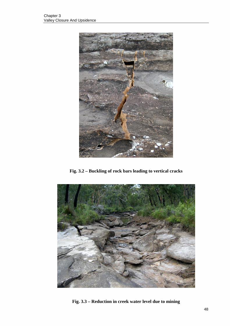
Chapter 3 Valley Closure And Upsidence
48
Fig. 3.2 – Buckling of rock bars leading to vertical cracks
Fig. 3.3 – Reduction in creek water level due to mining

Chapter 3 Valley Closure And Upsidence
49
To date, the most comprehensive review on valley closure and upsidence due to mining
was performed by Waddington Kay and Associates as part of ACARP Project
No. C9067. These research reports culminated in a handbook for the undermining of
cliffs, gorges and river systems (Waddington Kay & Associates, CSIRO Petroleum
Division & University of New South Wales 2002) and contain a conceptual model for
valley closure and upsidence, along with an empirical method to predict valley closure,
upsidence, compressive strain and regional horizontal movement for river valleys that
have been undermined.
3.2 CURRENT MODELS 3.2.1 Horizontal stress model
In Waddington Kay and Associates (2002), it is summarised that during the formation
of a river valley, the horizontal stresses in the valley sides redistribute to the valley base,
causing an increase in horizontal compressive stress. This phenomenon is not new and
is commonly referred to as the ‘notch effect’. As the base of the valley is a free surface,
it is able to expand vertically. This upward movement of the valley base is generally
termed upsidence. Upward movement also occurs in the sides of the valley and for some
distance beyond.
When a river valley is directly undermined by a longwall panel, the conceptual model
stipulates that the longwall panel extraction causes a redistribution of horizontal
compressive stress above and below the mined out seam. The horizontal compressive
stress that is distributed below the longwall panel contributes to buckling and failure of
the floor of the extraction, whilst the horizontal compressive stress distributed above the
longwall panel adds to the already high horizontal compressive stress at the base of the
valley. This conceptual model is illustrated in Figure 3.4.
Depending on the bedding plane spacing and strength of rock in the valley base, the
increase in horizontal compressive stress may be enough to buckle and fail the valley
base (Figure 3.5 and Figure 3.6). Failure of the strata in the valley base continues
downwards until equilibrium is achieved. This can occur if a stronger bed is reached or
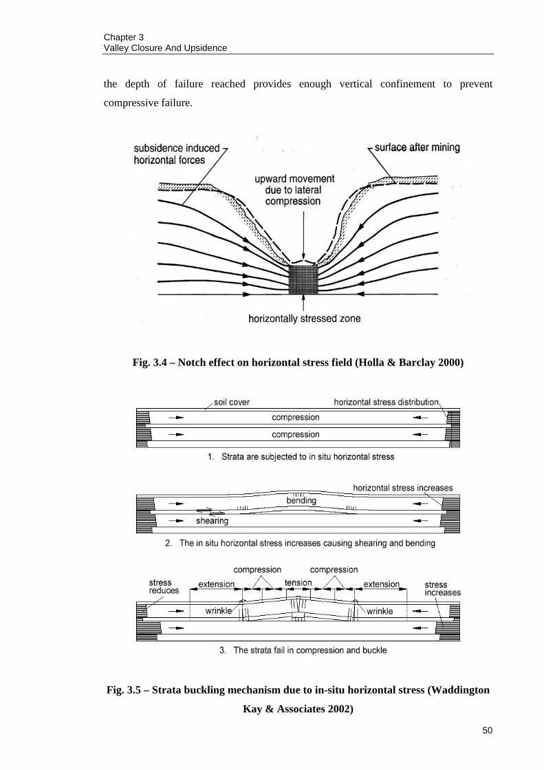
Chapter 3 Valley Closure And Upsidence
50
the depth of failure reached provides enough vertical confinement to prevent
compressive failure.
Fig. 3.4 – Notch effect on horizontal stress field (Holla & Barclay 2000)
Fig. 3.5 – Strata buckling mechanism due to in-situ horizontal stress (Waddington
Kay & Associates 2002)

Chapter 3 Valley Closure And Upsidence
51
Fig. 3.6 – Possible failure mechanisms in the bottom of a valley (Waddington Kay
& Associates 2002)
The buckling and failure of the valley base can create voids below the base of the
valley. This failure of the valley base allows some relaxation of the sides of the valley to
occur, resulting in valley closure.
3.2.2 Empirical predictions
In Waddington Kay and Associates (2002), an empirical method to predict valley
closure and upsidence has been developed. This method is based on upper-bound
measured values and is anticipated to over-predict in areas of lower horizontal stress.
The prediction method for valley closure and upsidence is based on a series of graphs
that show the interrelationships between closure/upsidence and a number of
contributory factors. The contributing factors include:
Longitudinal distance from travelling, commencing or finishing goaf end,
Valley depth (incised gorges), and
Maximum incremental subsidence of mined longwall panel.

Chapter 3 Valley Closure And Upsidence
52
The contributing factors are plotted on graphs and serve as adjustment factors to predict
valley closure and upsidence.
The distance measurement convention used in the predictions is shown in Figure 3.7.
Fig. 3.7 – Distance measurement convention for valley closure and upsidence
predictions (Waddington Kay & Associates 2002)
The transverse distances for points A, B, C and D in Figure 3.7 are -270 m, 115 m,
460 m and 680 m respectively. Distances outside the goaf are negative. The longitudinal
distances for points A, B, C and D are 450 m, 350 m, 160 m and -130 m respectively.
Distances outside the goaf are also negative.
The graphs used to predict valley closure are shown in Figures 3.8 to 3.11 and the
graphs used to predict upsidence are shown in Figures 3.12 to 3.15. The base data used
to prepare these plots are not available in the literature. It is also important to note that

Chapter 3 Valley Closure And Upsidence
53
the plots include the raw data (blue) as well as so called adjusted data that was produced
by Waddington Kay and Associates in the formulation of their empirical models.
To make a prediction of valley closure or upsidence at a point in the base of a creek or
river valley, the following information is necessary:
Distance of the point from the advancing edge of the longwall panel,
Longitudinal distance from the nearest end of the longwall panel,
Valley depth,
Maximum incremental subsidence of the longwall panel that is being mined, and
Longwall panel and pillar widths.
The initial prediction of valley closure is made using Figure 3.8. The value of valley
closure is then adjusted by multiplying it by the adjustment factors obtained in Figures
3.9 to 3.11. The procedure followed for predicting upsidence is the same as predicting
valley closure.
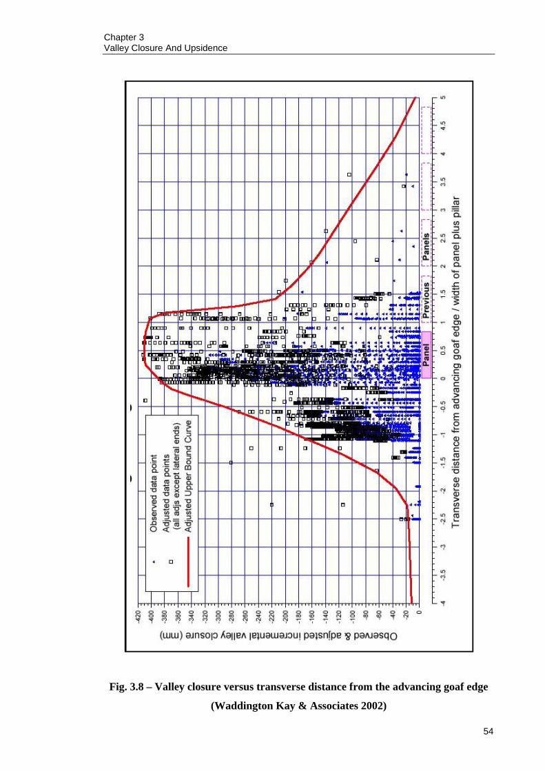
Chapter 3 Valley Closure And Upsidence
54
Fig. 3.8 – Valley closure versus transverse distance from the advancing goaf edge
(Waddington Kay & Associates 2002)

Chapter 3 Valley Closure And Upsidence
55
Fig. 3.9 – Valley closure adjustment factor versus longitudinal distance
(Waddington Kay & Associates 2002)
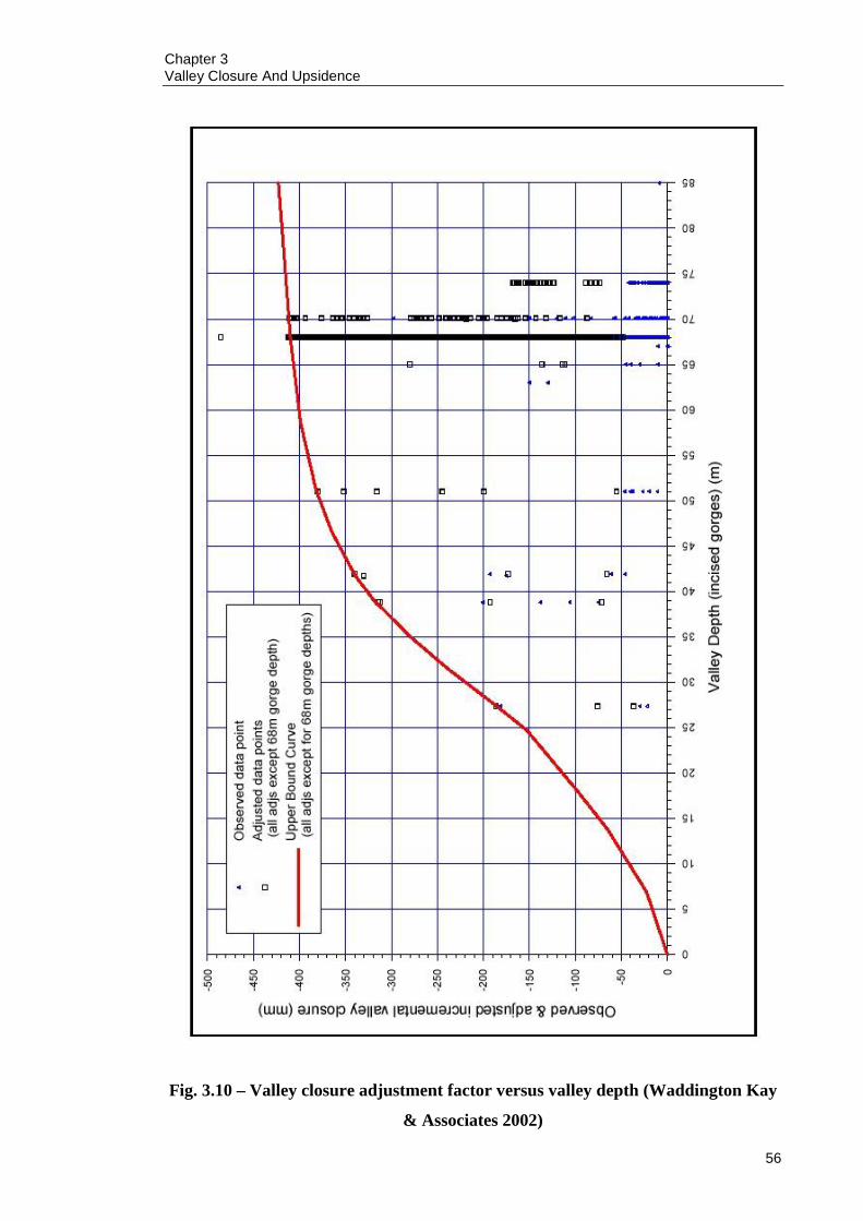
Chapter 3 Valley Closure And Upsidence
56
Fig. 3.10 – Valley closure adjustment factor versus valley depth (Waddington Kay
& Associates 2002)
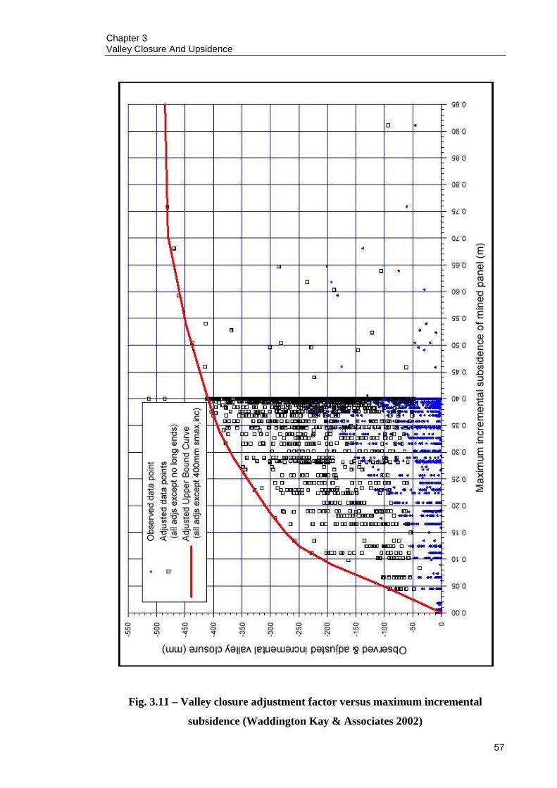
Chapter 3 Valley Closure And Upsidence
57
Fig. 3.11 – Valley closure adjustment factor versus maximum incremental
subsidence (Waddington Kay & Associates 2002)
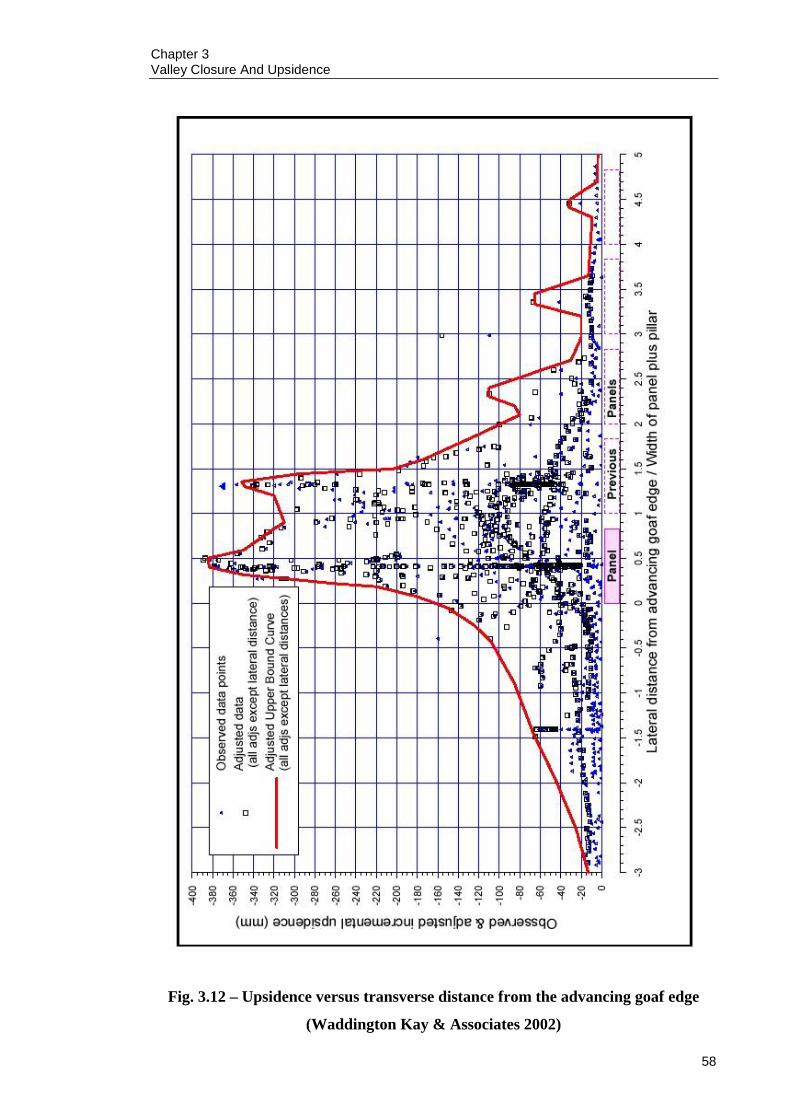
Chapter 3 Valley Closure And Upsidence
58
Fig. 3.12 – Upsidence versus transverse distance from the advancing goaf edge
(Waddington Kay & Associates 2002)

Chapter 3 Valley Closure And Upsidence
59
Fig. 3.13 – Upsidence adjustment factor versus longitudinal distance (Waddington
Kay & Associates 2002)

Chapter 3 Valley Closure And Upsidence
60
Fig. 3.14 – Upsidence adjustment factor versus valley depth (Waddington Kay &
Associates 2002)

Chapter 3 Valley Closure And Upsidence
61
Fig. 3.15 – Upsidence adjustment factor versus maximum incremental subsidence
(Waddington Kay & Associates 2002)

Chapter 3 Valley Closure And Upsidence
62
3.2.3 Limitations
For a river valley that is directly undermined by a longwall panel, the horizontal stress
model is valid. By virtue of geometry, it would be expected that horizontal stresses are
predominately compressive in the base of a valley that is located in the sagging portion
of the subsidence profile. Results from the empirical study (Waddington Kay &
Associates 2002) show that cases of valley closure and upsidence occur well outside the
goaf edge in unmined coal and also over old longwall panels (Figure 3.8 and
Figure 3.12). These events largely occur in the hogging portion of the subsidence
profile, where the horizontal stresses are predominately tensile.
The significance of these valley closure and upsidence events above unmined coal is
considerable. There is an increase in the environmental footprint, which is usually
seized upon by environmental, community and anti-mining groups. The increase in
environmental footprint may lead to problems in defining the limit of mining influence
using the traditional 20 mm vertical subsidence cut-off limit. This in turn potentially
leads to policies defining mining barriers and stand-off distances, as environmental
groups like the RIVERS SOS coalition seek the establishment of a one kilometre
protection zone around rivers in the Southern Coalfield (Mineral Policy Institute 2005).
Mining barriers lead to increased roadway development to access coal reserves on the
other side of protected rivers, and these results in inefficient mine designs and most
importantly, sterilisation of coal reserves. An example of this can be seen in
Figure 3.16, which illustrates BHP Billiton Illawarra Coal’s original mine layout for the
Douglas Project which undermined the Nepean River, and the amended layout which
does not undermine the Nepean River at all (BHP Billiton 2005).

Chapter 3 Valley Closure And Upsidence
63
Plan for discussion
Final layout
Fig. 3.16 – Original and amended plan for mining near the Nepean River (BHP
Billiton 2005)
The conceptual model of redistributed horizontal compressive stress in two dimensions
cannot explain the upsidence and closure events in the hogging phase, the lack of valley
closure and upsidence over currently mined longwall panels, or explain why valley
closure occurs if there is no valley base failure. It is simply not sufficient to assume that

Chapter 3 Valley Closure And Upsidence
64
all valley closure and upsidence events occur because of horizontal compressive stress.
It is also not sufficient to assume that valley closure and valley base failure are related.
3.2.4 Recent developments
A review was published on the Southern Coalfield Enquiry (SCI) in July 2008 (NSW
Department of Planning 2008). This independent enquiry was established because of
concerns held by the NSW Government over both past and potential future impacts of
mine subsidence on significant natural features in the Southern Coalfield. These
concerns first surfaced in the community in 1994 when the bed of the Cataract River
suffered cracking and other subsidence impacts.
The enquiry conducted a state of the art review of subsidence impacts of significant
natural features and recognised the fact that valley closure and upsidence in the far-field
are difficult to predict, and the mechanisms are not fully understood.
A review of the mechanisms behind valley closure and upsidence referenced the
horizontal compressive stress model of Waddington Kay and Associates (2002) as the
most likely mechanism if the valley is located above the mining area. It was recognised
that valley closure and upsidence in the far field was not fully understood. The
following possible mechanisms were listed but not expanded upon:
Simple elastic horizontal deformation of the strata within the exponential ‘tail’
of the subsidence profile that applies in conventional circumstances,
Influence of valleys and other topographical features which remove constraints
to lateral movement and permit the overburden to move en masse towards the
goaf area, possibly sliding on underlying weak strata layers,
Unclamping of near-surface horizontal shear planes,
Influence of unusual geological strata which exhibit elasto-plastic or time
dependant deformation,
Stress relaxation towards mining excavations,
Horizontal movements aligned with the principal in-situ compressive stress
direction,
Valley notch stress concentrations,

Chapter 3 Valley Closure And Upsidence
65
Movements along regional joint sets and faults, and
Unclamping of regional geological plates.
It was concluded that the coal mining industry should escalate research into the
prediction of non-conventional subsidence effects in the Southern Coalfield and their
impacts and consequences for significant natural features, particularly in respect of
valley closure, upsidence and other topographical features.
Shortly after the conclusion of the enquiry, The Metropolitan Coal Project Review
Report was published (NSW Planning Assessment Commission 2009). This report
contained the proposal known as the Metropolitan Coal Project, which related to the
future life of mine planning for Metropolitan Colliery. It is the first mining proposal in
the Southern Coalfield since the SCI was published in 2008.
A review of subsidence and far-field events like valley closure and upsidence was
conducted but mostly drew from the SCI. This illustrates that progress on identifying
and verifying a mechanism that explains valley closure and upsidence events over
unmined coal is not progressing swiftly.
3.3 ALTERNATIVE MODEL
Due to the inability of the horizontal compressive stress model to explain upsidence and
valley closure over unmined coal and old longwall panels, the new conceptual model
involves investigating whether block movements in the sagging phase contributes to
upsidence and valley closure in the hogging phase.
The basic concept of this model is illustrated in Figure 3.17.

Chapter 3 Valley Closure And Upsidence
66
Fig. 3.17 – New conceptual model for upsidence and valley closure in the hogging
phase
This conceptual model proposes that if a translation plane is present at the base of the
valley, the closure observed above unmined coal is a result of rock blocks being pushed
into the void provided by the valley, due to the horizontal shortening of the ground
surface directly above the mined longwall panel. Upsidence is not expected to occur due
to the translation plane dissipating any built up horizontal stress generated by the
movement of the blocks.
If the translation plane is not present at the base of the valley, but located beneath the
base of the valley, it is proposed that upsidence will be the dominant feature present
above unmined coal. Rock blocks will still have horizontal stresses exerted on them by
the horizontal shortening of the ground surface, forcing them in an outward direction,
but as no translation plane exists to dissipate the horizontal stress, there will be a
concentration in horizontal compressive stress at the base of the valley causing
upsidence, and possibly valley base failure. It is anticipated that valley closure above
unmined coal is a function of translation plane location, curvature of the ground surface
and valley depth. Likewise, upsidence above unmined coal is thought to be a function of
translation plane location and curvature of the ground surface.
Valley closure in hogging mode – a number of cases reported
Tensile conditions theoretically anticipated Block movements, i.e. blocks pushed uphill?

Chapter 3 Valley Closure And Upsidence
67
The assumption that a translation plane exists below the ground surface is based on
what is reported in the literature. In Holla and Barclay (2000), it is reported that surface
wrinkles at Tahmoor Colliery were a result of a plane of weakness below the ground
surface. It was also reported that a nearby borewell was damaged by horizontal shearing
of the borehole wall.
A similar occurrence was also reported in Mills and Huuskes (2004) where monitoring
instruments in a valley base at Metropolitan Colliery were replaced due to horizontal
shearing. In a previous report by Mills (2002) it was noted that there was a loss of
drilling water recirculation and low RQD observed in the core at around 6 m below the
base of the valley in the same area.
In Holla and Armstrong (1986), it was reported that a borehole at West Cliff Colliery
became impassable to a logging probe at 80 m below the ground surface.
This proposed model is compatible with the data in the empirical method described
earlier in this chapter as it will provide an explanation for valley closure and upsidence
over unmined coal and old longwall panels and take into account the presence of a
translation plane below and at the base of a valley.
3.3.1 Kinematics of a particle moving along a known path The kinematics of a particle moving along a known path is described in this section and
is reproduced from Hibbeler (1997). The main principle can be readily adapted to
blocks moving along a known path, i.e. the subsidence profile.
Planar motion
Consider the particle P shown in Figure 3.18, which is moving in a plane along a fixed
curve, such that at a given instant it is located at position s, measured from point O.
Consider a coordinate system that has its origin at a fixed point on the curve, and at the
instant considered this origin happens to coincide with the location of the particle. The t
axis is tangent to the curve at P and is positive in the direction of increasing s. This
positive direction is designated with the unit vector ut. A unique choice for the normal
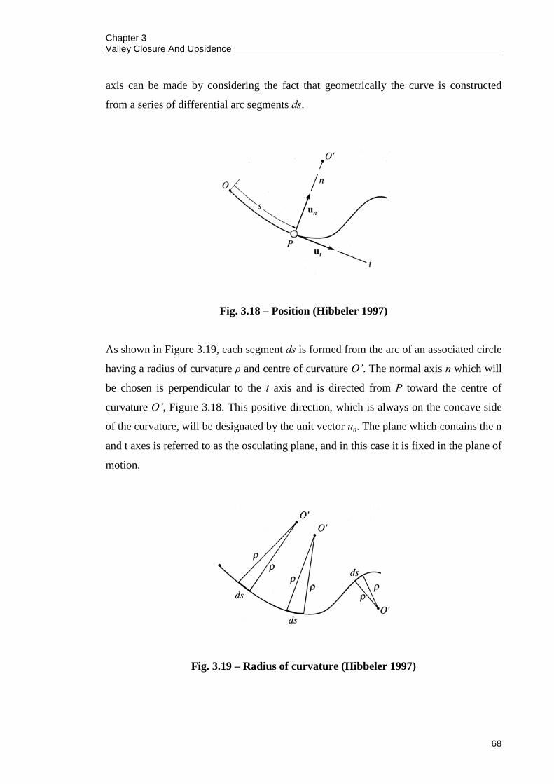
Chapter 3 Valley Closure And Upsidence
68
axis can be made by considering the fact that geometrically the curve is constructed
from a series of differential arc segments ds.
Fig. 3.18 – Position (Hibbeler 1997)
As shown in Figure 3.19, each segment ds is formed from the arc of an associated circle
having a radius of curvature ρ and centre of curvature O’. The normal axis n which will
be chosen is perpendicular to the t axis and is directed from P toward the centre of
curvature O’, Figure 3.18. This positive direction, which is always on the concave side
of the curvature, will be designated by the unit vector un. The plane which contains the n
and t axes is referred to as the osculating plane, and in this case it is fixed in the plane of
motion.
Fig. 3.19 – Radius of curvature (Hibbeler 1997)

Chapter 3 Valley Closure And Upsidence
69
Velocity
Since the particle is moving, s is a function of time. The particle’s velocity v has a
direction that is always tangent to the path, Figure 3.20, and a magnitude that is
determined by taking the time derivative of the path function s = s(t), i.e. v = ds/dt
(Equation 3.1 and Equation 3.2).
Hence,
tuv υ= [3.1]
Where,
•
= sυ [3.2]
Fig. 3.20 – Velocity (Hibbeler 1997)
Acceleration
The acceleration of the particle is the time rate of change of the velocity (Equation 3.3),
tt uuva•••
+== υυ [3.3]

Chapter 3 Valley Closure And Upsidence
70
In order to compute the time derivative tu•
, note that as the particle moves along the arc
ds in time dt, ut preserves its magnitude of unity; however, it changes its direction, so
that it becomes 'tu , Figure 3.21.
Fig. 3.21 – Time derivative (Hibbeler 1997)
As shown in Figure 3.22, we require ttt duuu +=' . Here dut stretches between the
arrowheads of ut and 'tu , which lie on an infinitesimal arc of radius 1=tu . Hence dut has
a magnitude of ( ) θddut 1= , and its direction is defined by un.
Fig. 3.22 – Time derivative components (Hibbeler 1997)

Chapter 3 Valley Closure And Upsidence
71
Consequently, nt uddu θ= , and therefore the time derivative becomes nt uu••
= θ . Since
θρdds = , then ρθ••
= s , and consequently (Equation 3.4),
nnnt uusuuρυ
ρθ ===
•••
[3.4]
Substituting into Equation 3.3, a can be written as the sum of its two components
(Equations 3.5 to 3.7),
nntt uauaa += [3.5]
Where,
•
= υta or dsdat
υυ= [3.6]
and,
ρυ 2
=na [3.7]
These two mutually perpendicular components are shown in Figure 3.23, in which case
the magnitude of acceleration (Equation 3.8) is the positive value of:
22nt aaa += [3.8]
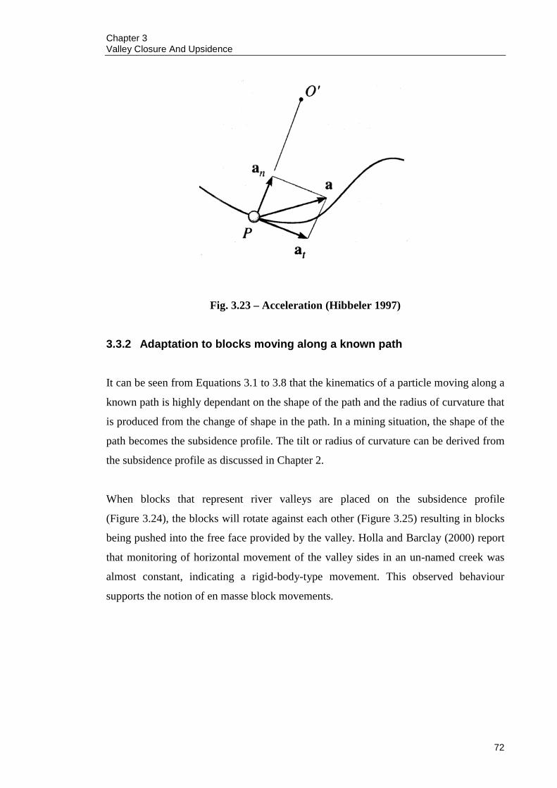
Chapter 3 Valley Closure And Upsidence
72
Fig. 3.23 – Acceleration (Hibbeler 1997)
3.3.2 Adaptation to blocks moving along a known path
It can be seen from Equations 3.1 to 3.8 that the kinematics of a particle moving along a
known path is highly dependant on the shape of the path and the radius of curvature that
is produced from the change of shape in the path. In a mining situation, the shape of the
path becomes the subsidence profile. The tilt or radius of curvature can be derived from
the subsidence profile as discussed in Chapter 2.
When blocks that represent river valleys are placed on the subsidence profile
(Figure 3.24), the blocks will rotate against each other (Figure 3.25) resulting in blocks
being pushed into the free face provided by the valley. Holla and Barclay (2000) report
that monitoring of horizontal movement of the valley sides in an un-named creek was
almost constant, indicating a rigid-body-type movement. This observed behaviour
supports the notion of en masse block movements.

Chapter 3 Valley Closure And Upsidence
73
Fig. 3.24 – Magnified block displacements on curved slope (after Nemcik 2003)
Fig. 3.25 – Area of contact between rotating blocks (Nemcik 2003)
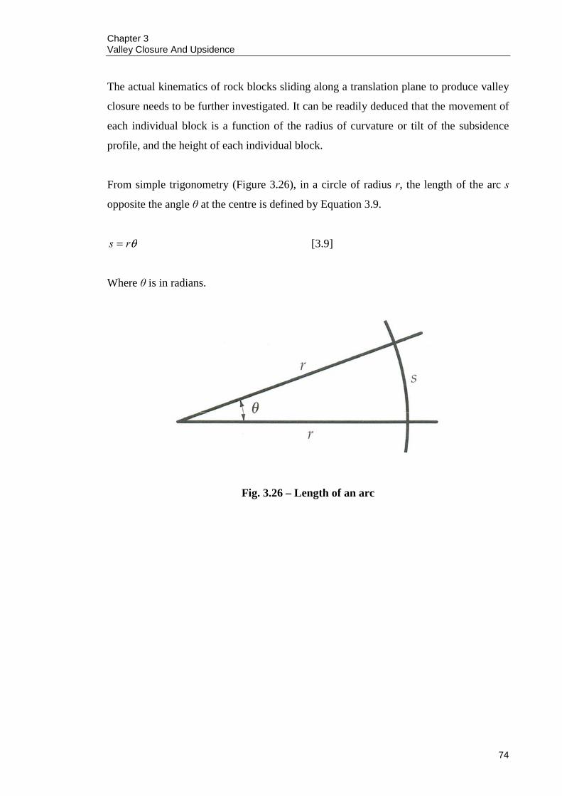
Chapter 3 Valley Closure And Upsidence
74
The actual kinematics of rock blocks sliding along a translation plane to produce valley
closure needs to be further investigated. It can be readily deduced that the movement of
each individual block is a function of the radius of curvature or tilt of the subsidence
profile, and the height of each individual block.
From simple trigonometry (Figure 3.26), in a circle of radius r, the length of the arc s
opposite the angle θ at the centre is defined by Equation 3.9.
θrs = [3.9]
Where θ is in radians.
Fig. 3.26 – Length of an arc

Chapter 3 Valley Closure And Upsidence
75
Adapting the above theory to block rotations and simplifying to enable simple
trigonometric analysis (Figure 3.27):
Fig. 3.27 – Exaggerated view of valley tilt and resulting closure
Where,
R1 = Depth of valley (m)
φ1 = Tilt of block adjacent to valley (radians)
C1 = Closure from one side of valley (m)
To determine the tilt experienced by one half of a valley, consider Figure 3.28.
Fig. 3.28 – Components of valley tilt
φ1
φ1 φ1
C1
Side of valley R1
x1
y1 y11
φ1

Chapter 3 Valley Closure And Upsidence
76
Where,
y1 = Subsidence at corner of block (m)
y11 = Subsidence at corner of block (m)
x1 = Distance between block corners (m)
Using simple trigonometry, the angle of tilt can be calculated from Equation 3.10 and
Equation 3.11, and the resulting closure can be calculated from Equation 3.12.
1
1111tan
xyy −
=φ [3.10]
1
1
1111 tan −⋅⎟⎟
⎠
⎞⎜⎜⎝
⎛ −=
xyyφ [3.11]
⎥⎦
⎤⎢⎣
⎡⋅⎟⎟⎠
⎞⎜⎜⎝
⎛ −= −1
1
11111 tan
xyyRC [3.12]
If the expression for φ1 in Equation 3.11 is substituted into Equation 3.12, it can be seen
that the final expression for closure takes on the form of Equation 3.9.
Equation 3.12 could possibly be used to calculate the inward closure of the valley wall
that is furthest from the longwall panel, as the proposed block movement mechanism
postulates that the side of the valley closest to the longwall panel is pushed away from
the longwall panel and into the free face provided by the valley, hence adding
displacements along the translation plane as an extra consideration. An exception would
be when the valley is located directly above the longwall panel, and then Equation 3.12
could be used to calculate the inward displacement of both walls, and hence total valley
closure.

Chapter 3 Valley Closure And Upsidence
77
3.4 REQUIRED WORK PROGRAM
As the alternative block movement model does not need to consider out-of-plane
stresses, it is amenable to two-dimensional numerical modelling. Therefore, it is
proposed to investigate the alternative block movement theory by numerical modelling.
In order for this to occur, the viability and credibility of the models created by the
chosen numerical code needs to be established.
The numerical modelling will take place in two stages. The first stage will involve the
creation of single longwall panel subsidence models that can be verified with the DPI
Southern Coalfield empirical method and analytical methods.
The second stage will involve the creation of simplified subsidence models that
incorporate river valleys and translation planes at different depths. These models will be
based on the single longwall panel subsidence models for consistency.
An emphasis will be placed on the models being transparent for credibility purposes. All
the material properties, assumptions and processes used in the creation of the models
will be fully traceable so that the results from the models will be beyond reproach.
3.5 SUMMARY
The widely accepted conceptual model was reviewed and it was quickly identified that
this model cannot explain upsidence and valley closure over unmined coal, a
phenomenon that is evident in the field data gathered by Waddington Kay and
Associates (2002). A review of recent developments revealed that no substantial
progress has been made in identifying the mechanism behind valley closure and
upsidence above unmined coal. The proposed alternative explanation of block
movements was introduced and is the subject of further investigation using numerical
modelling in the following chapters.

Chapter 4 Development Of A Numerical Modelling Approach
78
CHAPTER 4 DEVELOPMENT OF A NUMERICAL MODELLING
APPROACH
4.1 INTRODUCTION The numerical modelling of a geotechnical engineering problem can often be fraught
with uncertainties not only about the choice of the model but also the choice of the
values of input parameters and quite often assumptions are made without proper
justification. In order to avoid falling into this trap, the proposed numerical modelling in
this thesis will be developed in accordance to the principles outlined in Hudson,
Stephansson and Andersson (2005). A literature review (in chronological order) of
numerical modelling in mining subsidence related problems is also undertaken to
determine what numerical modelling code is most suitable for the modelling of single
isolated longwall panels and river valleys. The audits for the numerical modelling in this
thesis can be found in Appendix A.
4.2 MODELLING PRINCIPLES
The development of a numerical modelling approach for isolated single longwall panels
and the block movement model is based on the principles outlined in Hudson,
Stephansson and Andersson (2005). The principles stipulate that the numerical
modelling itself is not the most important aspect, but the conceptualisation of the
problem, material properties and parameters should be paramount in any investigation.
It is also stressed that the engineering problem at hand should be subjected to ‘soft’ and
‘hard’ audits.
The soft audit establishes an overview of the modelling work and determines whether
well known issues of importance and difficulty in characterising and modelling rock
masses have been addressed at the outset. The hard audit is similar to the soft audit but
requires justifications to the answers given. The audits are designed to ensure that the
numerical modelling is transparent and traceable through the audit trail.

Chapter 4 Development Of A Numerical Modelling Approach
79
Several references that deal with numerical modelling of mining subsidence or mining
related activities with UDEC, FLAC or similar software are reviewed. The aim of this
chapter is to make a decision on which numerical code is better suited to modelling
mining induced subsidence for isolated single longwall panels and block movements
based on the examples given.
4.3 LITERATURE REVIEW
4.3.1 Coulthard and Dutton (1988)
In this paper, the numerical modelling programs FLAC and UDEC are used to calculate
the subsidence over a longwall panel for a range of longwall panel widths. The results
from the numerical modelling were compared to the empirical predictions for the NSW
Southern Coalfield.
Holla’s empirical work on subsidence prediction in the Southern Coalfield indicated
there was a large increase in the maximum developed subsidence as longwall panel
widths increase from subcritical to critical.
At the moment, there are no critical width longwall panels in the Southern Coalfield, but
the authors argue that subsidence prediction will only become feasible if it can capture
the subsidence characteristics for a range or different mining geometries and geological
conditions.
From the results of their numerical modelling, the authors reproduced the results of
earlier workers that dismissed elastic analyses because of the shallow subsidence profile
produced, and the unrealistic calibration of material properties required to fit the elastic
analyses to observed subsidence profiles.
On the other hand, it was found that modelling a non-linear material with FLAC,
containing horizontal ubiquitous joints, produced a large increase in the maximum
developed subsidence, as characterised by Holla’s work. It was also found that UDEC
produced this large increase as well.

Chapter 4 Development Of A Numerical Modelling Approach
80
In conclusion, the authors felt that both the FLAC and UDEC models have the potential
of predicting subsidence in new geological environments, but UDEC was favoured
because of its ability to model roof behaviour. The authors found that the key factors
governing the UDEC predictions were highly dependant on the material properties
(joint friction angle and elastic modulus of the rock mass) and jointing pattern selected
(finer upper strata increased subsidence magnitude).
4.3.2 Johansson, Riekkola and Lorig (1988)
In this paper, the authors discuss their experience in the design of multiple parallel
caverns using explicit finite difference methods. The two programs that were used were
FLAC and UDEC.
After the site characterisation was complete, preliminary modelling was performed on
several major cross sections using FLAC. The purpose of this preliminary modelling
was to identify potential areas where stability problems may arise. Once critical areas
were identified, more detailed analyses were performed. Where joint spacing was
relatively wide, UDEC was employed. Where rock was highly fractured, FLAC was
used.
The purpose of this paper was to demonstrate how valuable numerical modelling can be
in the design process.
4.3.3 Alehossein and Carter (1990)
In this paper, the authors discuss the difference between implicit and explicit modelling
of joints (horizontal and vertical) in a rock mass. The numerical model used is a simple
trench style excavation, with one-half of the problem discretised because of symmetry.
The rock material was assumed to be an isotropic, linear elastic material, and the joints
were assumed to conform to the elasto-plastic Mohr-Coulomb failure criteria. Joints
were modelled implicitly as part of the constitutive model, i.e. ubiquitous, and
explicitly. Joint spacing was varied in each model.

Chapter 4 Development Of A Numerical Modelling Approach
81
From the modelling of horizontal joints, it was found that jointing had little effect on
overall horizontal movements, and the predictions from both the implicit and explicit
modelling were quite close. On the other hand, it was found that vertical movement was
sensitive to explicit joint spacing, compared to implicit joint spacing. From the
modelling of vertical joints, it was found that both implicit and explicit joints produced
similar results.
In conclusion, the authors suggested that the computationally more efficient method of
implicit joint modelling was adequate for many practical problems. It was also noted
that the accuracy of the implicit method depended of the spacing of the joints relative to
a typical dimension of the excavation.
4.3.4 Brady et al. (1990)
In this paper, the authors used UDEC to model static and dynamic behaviour of jointed
rock. The results from the modelling were then compared with the analytical solutions.
Four problems have been used for the study. These included:
Jointed block subject to cyclical loading (static),
Circular excavation intersected non-diametrically by a joint (static),
Plane shear wave normally incident on a joint in an elastic solid (dynamic), and
Explosive source located near a slip-prone joint (dynamic).
The joint deformation model used in the analysis was the Coulomb strength model. In
all cases, the numerical simulation matched well with the analytical solutions.
From the results of the modelling, it was concluded that UDEC can simulate the
mechanics of jointed rock, but the study did not confirm that UDEC is a valid
simulation of the engineering behaviour of jointed rock.

Chapter 4 Development Of A Numerical Modelling Approach
82
4.3.5 Choi and Coulthard (1990)
In this paper, the authors examined the results of distinct element modelling applied to a
simple trap door problem, and compared the results with Cosserat continuum limit load
calculations. Distinct element studies of mining-induced subsidence were also
discussed.
The authors reviewed the three different methods of modelling a jointed rock mass:
explicit modelling, equivalent continuum modelling, and generalised continuum
modelling. The general conclusion drawn was that explicit modelling of joints is the
best method where block separation, rotation and slip, and large relative motions may
occur. Equivalent continuum models were regarded as unreliable unless the joint
spacings were very small compared with other system lengths. The generalised
continuum method was viewed as a somewhat promising approach, as it was able to
represent internal structure without being limited by the assumption that the structure is
very small relative to system lengths.
From the results of their numerical modelling with UDEC, the DE analysis matched the
Cosserat continuum method for the active case (simple mechanism), but not for the
passive case (complex mechanism). It was concluded that for the passive case, the
material in the upper part of the model should be treated as a continuum.
It was concluded that a discontinuum can be modelled as a generalised continuum
where the structure is reasonable simple and the assumed mechanism is correct. If the
structure is more complex and the mechanism not easily predicted, distinct element
methods or finite element methods (incorporating the Cosserat theory) should be used.
The authors then discussed the applicability of distinct element modelling to subsidence,
with reference to the Angus Place Case Study. Again, elastic models were discounted as
reliable means of subsidence prediction due to their inability to model roof strata
behaviour. The credibility of distinct element models was demonstrated by the
comparison of DE modelling results and physical models in Australian rock conditions.
Chapter 4 Development Of A Numerical Modelling Approach
83
It was found that the major factors affecting the results of the UDEC modelling were the
suitable spacing of bedding planes and sub-vertical jointing. Even so, the UDEC
modelling matched the trends in surface subsidence better than continuum models. It
was also noted that the method of excavation may produce different behaviour.
4.3.6 O’Conner and Dowding (1990)
In this paper, the authors described their findings from numerical modelling which
complemented a field study that carried out extensive deformation measurements during
the excavation of a longwall panel. The purpose of the numerical modelling was to try
and simulate mining induced subsidence and to demonstrate the influence of
discontinuities on the rock mass.
The authors used a hybrid code that combined the Northwestern University Rigid Block
Model with the rigid block model developed by Peter Cundall. The main feature of this
hybrid code is the edge-to-edge contacts between blocks. When all the edge-edge
contacts of a block have satisfied one of three failure criteria (pure tensile failure, shear
failure and rotation-tension failure) the block can undergo large displacements and
rotations and develop corner-edge contact with any other block.
The subsidence model was based on a transverse cross section of the longwall panel.
The bedding planes were approximated from borehole geophysics and mapping data.
The joint sets were obtained from mapping of rock exposures. Six different scenarios
were carried out, and these varied the number of strata types, joint and bedding plane
stiffness, joint density, and shear resistance.
In conclusion, the authors found that the rigid block model was capable of simulating
the general trend of vertical displacements within the overburden, but could not
simulate fracturing and shearing above the zone of block caving. It was also found that
the rigid block model behaved more stiffly than the actual rock mass, and consequently,
the models which contained relatively low stiffness values produced the best agreement
between measured and calculated displacements. Lastly, it was found that increasing the
density of vertical joints or reducing the rigid block contact roughness did not improve
the agreement between measured and simulated displacements.

Chapter 4 Development Of A Numerical Modelling Approach
84
4.3.7 Coulthard (1995)
In this paper, Coulthard reported on his work from the Angus Place Case Study. In this
study, several scientists and engineers were invited to predict the developed subsidence
over two longwall panels mined in virgin coal. The author chose UDEC to develop
numerical models and subsidence predictions.
The author justified his choice of program by discussing the fact that distinct element
methods such as UDEC can model the discontinuum behaviour that forms a key part of
the mechanical response of a rock mass to longwall mining. The purpose of this study
was to evaluate the potential of this numerical method for predicting subsidence in
environments where no empirical data are available.
Parameters that were changed in the model (to fine tune) included DE sizes and shapes
in the lower roof strata to produce bulking, joint constitutive model for sub-vertical
jointing, and the finite difference zoning within the blocks. It was noted that little
information was available on jointing in the rock mass apart from the sub-horizontal
bedding planes, therefore the model did not attempt to represent the detailed geology of
the rock strata. Average rock properties were used in all regions.
The blocks were governed by the Mohr-Coulomb elasto-plastic constitutive model. The
bedding planes were modelled as standard UDEC joints, with initial elastic behaviour
and with slip and separation determined by a Mohr-Coulomb shear strength criterion
with tensile cut-off. The sub-vertical joints were modelled with UDEC’s ‘intact rock’
constitutive model.
In conclusion, it was found that the UDEC analyses yielded good qualitative agreement
with the main aspects of the field measurements, including:
Magnitude and asymmetry of subsidence,
The narrowness of the subsidence peaks, and
Collapse of immediate roof strata and trends in deformations in the central
borehole.

Chapter 4 Development Of A Numerical Modelling Approach
85
The model was not calibrated after field results became available. It was also noted that
the model was able to produce asymmetry in the subsidence profile, something that was
not possible in an elastic continuum analysis.
The main limitations of the UDEC models were found to be:
Failure to reproduce bulking of the collapsed goaf,
Failure to match borehole displacements in the upper strata, and
Considerable underestimates of subsidence over the chain pillar.
It was proposed to increase the orientation of potential crack planes by defining multiple
sets of intersecting joints in the lower roof. It was suggested that this can allow some
block rotation to develop and increase the bulking of the goaf.
4.3.8 Bhasin and Høeg (1998)
In this paper, the authors performed a parametric study on the joint constitutive model
for a large cavern in the Himalayas using UDEC. The joint constitutive models that
were compared were the Mohr-Coulomb and the Barton-Bandis models. The results of
the parametric study indicated that deformations around an opening were dependant on
the size or the number of blocks adjacent to the excavation. It was also found that in a
model where the block size is small compared to the excavation dimensions, the failure
mechanism in jointed rock masses was strongly influenced by volume changes when
approaching failure, and these volume changes were generally determined by the
dilation along pre-existing discontinuities. This dilation along the joints caused a build-
up of high normal stresses which in underground openings can cause interlocking of the
blocks and inhibit further deformation. This situation may be relieved by using the
Mohr-Coulomb joint constitutive model instead of the Barton-Bandis model, as the
Barton-Bandis model allows for the build-up of stress caused by dilatant behaviour.
This may be particularly useful when modelling underground longwall excavations.

Chapter 4 Development Of A Numerical Modelling Approach
86
4.3.9 Alejano et al. (1999)
In this paper, the authors used FLAC to develop subsidence models for flat coal seam
longwall mining in British basins. These FLAC models were validated from empirical
methods (SEH). The authors also developed models for slightly inclined coal seams and
for steeply inclined coal seams. The slightly inclined coal seam models were also
validated by empirical observations, but the steeply inclined models were not. The
numerical models were based on longwall mines from the Midlands coalfields in central
England. There was a large amount of material properties data and empirical predictions
available.
The authors chose an elasto-plastic material model with the following features:
Transversely isotropic elastic pre-failure behaviour,
Anisotropic yield surface, yield may occur by joints or material itself, and
Isotropic elastic post-failure behaviour.
To assess the quality of the rock mass, the GSI rating was used. The strength parameters
of the Coal Measures rock mass were determined by the Hoek-Brown criterion, and
equivalent Mohr-Coulomb parameters calculated. Joint strength was determined by
scaling the results of laboratory testing.
The calculation of pre-failure (Ex, Ey, υxy, υyx and G) and post-failure deformability
parameters (E) relied on formulas suggested by several authors. It was stated that these
formulas simulated rock mass behaviour quite well. It was noted that the material model
described is not available in FLAC and must be implemented via subroutines written in
an in-built language (FISH).
The implementation of the material model followed a two stage process. First, an
isotropic elastic model was assigned to the rock mass, compatible with the ubiquitous
joint model. The FLAC model was then run in order to estimate the height of the
fractured zone. Any material lying above the fractured zone was then assigned a
transversely isotropic elastic model.

Chapter 4 Development Of A Numerical Modelling Approach
87
It was stated that forty two models were created for coal seams located at 150 m, 200 m,
300 m, 400 m, 500 m and 700 m depth with W/H ratios of 0.4, 0.6, 0.8, 1, 1.25, 1.5 and
2 for each depth. This covered the range of subcritical, critical and supercritical values
defined by the SEH.
From the results of the numerical modelling, it was found that the subsidence troughs
produced by FLAC fit the empirical observations quite well, with the maximum
differences always smaller than 10 % of the seam thickness. On the other hand,
horizontal displacements did not match well at all. It was found that the maximum
horizontal displacement for the supercritical case was overestimated, whilst for the
subcritical case the opposite took place. The authors suggested that the occurrence of
surface tension cracks may account for these differences, in effect turning a continuous
material into a discontinuous material.
Other parameters that were compared to SEH results were fractured zone height,
subsidence factor, rib-side subsidence, limit angle, and maximum horizontal
displacement in trough. It was stated by the authors that the FLAC results agree or
follow general trends given by the SEH results, with the exception of limit angle and
maximum horizontal displacement. The limit angle predicted by FLAC was within the
range of 30° – 45°, whereas the SEH assumed the limit angle to be constant at 35°. The
reasons for the difference in horizontal displacement had been covered previously.
In conclusion, the authors stated that subsidence due to longwall coal mining can be
adequately modelled by the described methodology, but there were still some issues to
be overcome. These included:
The problem of modelling a discontinuum with a continuum code. The authors
argued that given the large scale of the models involved, continuum modelling
can be representative of the actual rock mass behaviour. Also, it was pointed out
that discontinuum models had not been used successfully, most probably due to
the lack of knowledge about joint distribution,
The use of a custom constitutive model, whilst still effective, did not behave
exactly as required, and
Chapter 4 Development Of A Numerical Modelling Approach
88
Using rock characterisation techniques with accuracy with published data on
different Coal Measures rock masses.
4.3.10 Sitharam and Latha (2002)
In this paper, an equivalent continuum model had been incorporated into FLAC via the
FISH utility. The equivalent continuum model was verified with three case studies.
It was pointed out by the authors that the requirements for an equivalent continuum
model were Hoek & Brown parameters ‘s’ and ‘m’, JRC, JCS, and SRF (Barton and
Bandis model). Such parameters may not be readily available rendering the analysis of
such problems impossible. A new equivalent continuum approach was proposed, and
this approach required the estimation of only two joint parameters, namely the number
of joints in the rock per meter depth and the inclination of the most critical joint set.
These two parameters were used in conjunction with the joint roughness or strength
parameter to calculate the Joint Factor. The authors stated that the Joint Factor (Jf) can
take care of the effects of frequency, orientation and strength of joint. The Joint Factor
had been derived from extensive laboratory testing of intact and jointed specimens
(plaster of Paris, sandstone and granite).
In the model, the rock mass properties were determined by a set of empirical relations,
which expressed the elastic modulus of a jointed rock mass as a function of joint factor
and the elastic modulus of intact rock. The authors stated that this model had been
validated against experimental results and also with results from explicit modelling. It
was also stated that the model worked well for jointed rock masses with different joint
fabric and joint orientation.
The implementation of the model involved writing a FISH function that calculated the
elastic modulus of the jointed rock in the changing stress field. The function also
calculated the modulus ratio, the compressive strength ratio, and the confining pressure
of the rock mass. The constitutive model used was the Mohr-Coulomb model with a
confining stress dependant hyperbolic relation.

Chapter 4 Development Of A Numerical Modelling Approach
89
The model had been used in three case studies: two powerhouse excavations and one
mine excavation. The values of the joint factor ranged from 13 to 111. It was found that
the numerical analysis estimated the field behaviour very well. The authors concluded
that the joint factor model can be confidently applied for solving excavation problems in
jointed rock masses.
4.3.11 CSIRO Petroleum (2002)
Numerical modelling of undermined river valleys with UDEC and FLOMEC (three
dimensional continuum code) was performed by CSIRO Petroleum in order to replicate
observed behaviour in the Cataract and Nepean Gorges. Only the UDEC models will be
discussed as three dimensional modelling is beyond the scope of this thesis. The
modelling was carried out in two stages, the first being a geomechanical run, and the
second being a geomechanical fluid flow run.
Parametric variations to the UDEC geomechanical models included:
Gorge wall slope,
Joint strength,
Presence of ubiquitous joints,
Magnitude of horizontal in-situ stress,
Mining sequence, and
Bedding plane and vertical joint geometry.
Parametric variations to the UDEC geomechanical fluid flow models included:
Gorge wall slope,
Shallow river valley geometry,
Flat horizontal ground surface,
Additional parallel joint set in gorge wall, dipping 10 to 30 degrees,
Strength of 30 degree joints,
Ubiquitous joints in gorge wall dipping 30 degrees towards gorge,
Magnitude of horizontal in-situ stress,
Depth of water table,
Chapter 4 Development Of A Numerical Modelling Approach
90
Permeability of Bald Hill Claystone, and
Poro-elastic and steady state responses to mining.
In both cases, the parameters that were found to have the greatest effect on model
response were the magnitude of horizontal in-situ stress, the presence of ubiquitous
joints, joint strength and permeability. The authors concluded that the numerical
modelling provided greater understanding of general strata mechanisms that occurred
during the undermining of surface topographical features. It was also concluded from
the modelling that horizontal movements from valley closure induced by undermining
were predominately associated with bedding plane shear at shallow depth, and these
sheared bedding planes acted as conduits for ground water, and may impact on local
hydrology.
It was noted that the numerical models were not verified in any way, and although the
purpose of the exercise was to investigate valley closure outside longwall panels, no
explanation was given for why this occurred.
4.4 SUMMARY
From the reviewed references, the following points are deduced regarding numerical
modelling of mining induced subsidence:
Elastic models are considered unsuitable for subsidence prediction due to the
unrealistic calibration of material properties required in order to fit predicted
subsidence profiles to observed profiles,
Continuum codes like FLAC have been used to predict surface subsidence
successfully, but subsurface behaviour or horizontal movement cannot be
evaluated because of the continuum nature of the code,
It has also been shown that FLAC is unable to reproduce the large increase in
subsidence that occurs in the transition between subcritical and critical
extraction widths in the Southern Coalfield,
An equivalent continuum model has been produced, and it is claimed that it is
suitable for modelling jointed rock. This method seems to be limited to simple
excavations where large block movements are not expected,

Chapter 4 Development Of A Numerical Modelling Approach
91
It has also been demonstrated that the computationally more efficient method of
implicit joint modelling is adequate for many practical problems. It is also noted
that the accuracy of the implicit method depends of the spacing of the joints
relative to a typical dimension of the excavation. Again, this method is restricted
to simple problems where large block movements are not expected,
Distinct Element codes like UDEC were found to be generally more accurate
than FLAC because of their ability to model discontinuous rock masses,
therefore allowing evaluation of subsurface movements and roof behaviour,
Key factors governing UDEC predictions were highly dependant on the material
properties (joint friction angle and elastic modulus of the rock mass) and jointing
pattern selected (finer upper strata increased subsidence magnitude),
UDEC was able to produce asymmetry in the subsidence profile, something
which is not possible in an elastic continuum analysis (Angus Place Case Study),
UDEC modelling matched the trends in surface subsidence better than
continuum models. It was also noted that the method of excavation may produce
different behaviour (Angus Place Case Study), and
From UDEC verification studies, it is concluded that UDEC can simulate the
mechanics of jointed rock, but the study does not confirm that UDEC is a valid
simulation of the engineering behaviour of jointed rock.
From the above summary, it can be concluded that UDEC is the most suitable code to
develop a subsidence model in flat terrain and in areas of high topographical relief,
provided verification can be undertaken. Even though FLAC has the capability of
predicting surface subsidence quite well with equivalent continuum routines, the
incorporation of such a routine introduces a range of additional parameters that have to
be estimated, which in turn introduces a higher degree of uncertainty. Poor correlation
with horizontal movements restricts the use of FLAC in modelling undermined river
valleys due to resultant valley closure and horizontal movement of rock blocks.
Furthermore, UDEC has the advantage of being able to incorporate field properties
directly into the model without calibration, eg. in-situ stress field, bedding plane
spacing, joint spacing, sub vertical joint orientation, material and joint properties.

Chapter 5 Single Longwall Panel Models With No River Valley
92
CHAPTER 5 SINGLE LONGWALL PANEL MODELS WITH NO
RIVER VALLEY
5.1 INTRODUCTION
In this chapter, the approach used for modelling single longwall panel extractions in flat
terrain is developed and discussed. The selection of single longwall panel extractions
for modelling was such that it can be verified by the empirical method developed by
Holla and Barclay (2000), which was discussed in Chapter 2. The results from the
models are also discussed. An example of the modelling script used can be found in
Appendix B.
5.2 NUMERICAL MODELLING STRATEGY
The approach used in the numerical modelling of single longwall panels in flat terrain
was to try and replicate the DPI empirical model (single longwall prediction) in an
attempt to see whether UDEC was capable of modelling a relatively complex process
without the extensive calibrations that are sometimes required to get a model to ‘fit’
empirical observations. This step was necessary as it established the credibility of the
numerical models, and also provided a base on which river valleys can be modelled (in
terms of subsidence and curvatures).
Holla and Barclay (2000) provided a list of mines and extraction details, from which
ground movement data were collected and the subsidence curves derived (single
longwall panel only). The majority of the mines extracted the Bulli Seam using the
longwall method of mining. The data that was derived from pillar extraction and
Wongawilli Seam extraction was excluded from the modelling. It should be noted that
the extraction details are approximate figures only.
Holla and Barclay (2000) also provided the thickness of the stratigraphic units in the
overburden, grouped according to colliery. This was used for the derivation of the

Chapter 5 Single Longwall Panel Models With No River Valley
93
thickness of rock units above the Bulli seam for different mines. The details for the
rock units below the Bulli seam was derived from the literature and field geotechnical
characterisations.
5.3 MATERIAL PROPERTIES FOR INTACT ROCK
A great deal of information has been published on the material properties of the
stratigraphic units above and including the Bulgo Sandstone (Pells 1993). Most of this
data is derived from civil engineering works in and around Sydney, not specifically the
Southern Coalfield. A Mohr-Coulomb constitutive model has been used and this will be
continued. Most recently, a drilling program has been completed which contains the
geotechnical characterisation of several boreholes that were drilled over Appin and
Westcliff collieries (MacGregor & Conquest 2005). This geotechnical characterisation
resulted in a complete set of material properties for the:
Hawkesbury Sandstone,
Bald Hill Claystone,
Bulgo Sandstone,
Scarborough Sandstone,
Coal Cliff Sandstone, and
Loddon Sandstone.
UDEC requires the following material properties to be defined (for the Mohr-Coulomb
block model):
Density (kg/m3),
Young’s Modulus (GPa),
Poisson’s Ratio,
Bulk Modulus (GPa),
Shear Modulus (GPa),
Friction Angle (˚),
Dilation Angle (˚),
Cohesion (MPa), and
Tensile Strength (MPa).
Chapter 5 Single Longwall Panel Models With No River Valley
94
Typically, the parameters derived from multi-stage triaxial testing are Young’s
Modulus, unconfined compressive strength, Poisson’s Ratio, friction angle and
cohesion. The Mohr-Coulomb block model allows a specification of a dilation angle,
but if none is specified then the value used defaults to zero, i.e. for plastic yield to be
treated via a non-associated flow rule. In the absence of other information the dilation
angle has been set to zero. The other parameters such as bulk and shear moduli, and
tensile strength can be derived from formulae or tables (McNally 1996).
Complete material properties were missing for the Newport Formation, Bulli Seam and
Cape Horn Seam. The Stanwell Park Claystone, Wombarra Shale and Kembla
Sandstone were missing the values for friction angle and cohesion. The material
properties for the Balgownie Seam, Lawrence Sandstone, Cape Horn Seam, UN2,
Hargraves Coal Member, UN3, and the Wongawilli Seam were also derived. For
simplicity, the Balgownie Seam and Hargraves Coal member were assumed to have the
same material properties as the Bulli Seam, and the Lawrence Sandstone was assumed
to have the same material properties as the Loddon Sandstone.
Density
The densities of the various stratigraphic units have been well defined in the
geotechnical characterisation (MacGregor & Conquest 2005) and Pells (1993). The
density of coal was assumed to be 1500 kg/m3 (CSIRO Petroleum 2002). The densities
of UN2 and UN3 were derived from the sonic logs that formed part of the geotechnical
characterisation.
Unconfined Compressive Strength (UCS)
The missing UCS values were obtained by an examination of the sonic UCS for the
relevant borehole. MacGregor and Conquest (2005) provide an exponential relationship
(Equation 5.1) between the inferred UCS and the 20 cm field sonic velocity (VL2F).
This relationship is based on 142 samples established by BHP Illawarra Coal.
( ))200094.03217.1 FVLEXPSInferredUC ××= [5.1]
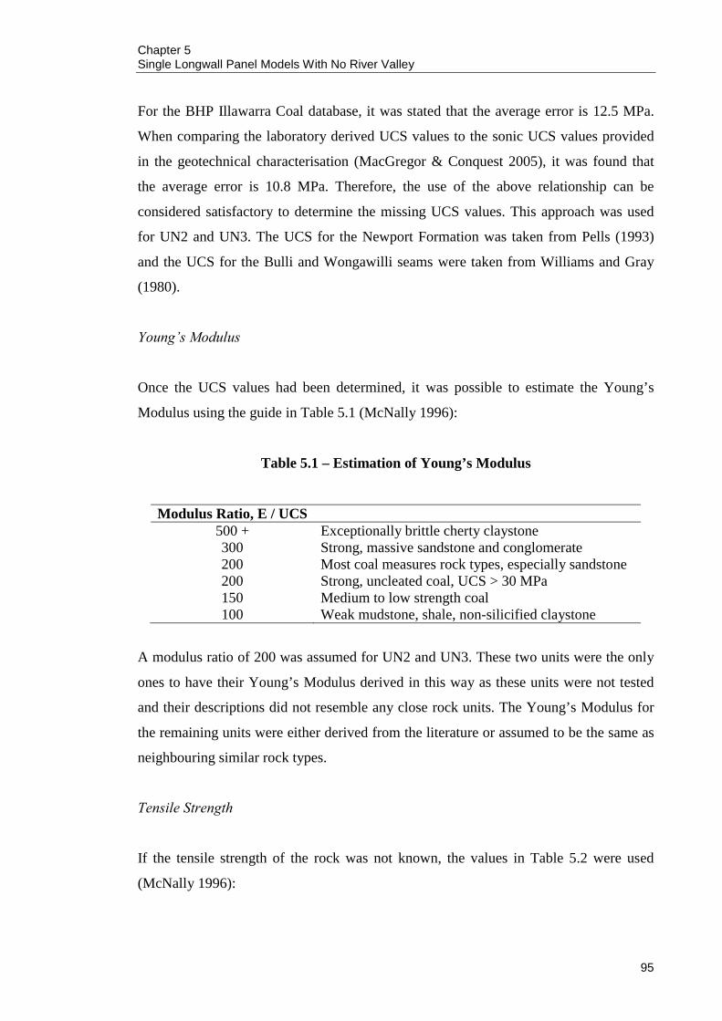
Chapter 5 Single Longwall Panel Models With No River Valley
95
For the BHP Illawarra Coal database, it was stated that the average error is 12.5 MPa.
When comparing the laboratory derived UCS values to the sonic UCS values provided
in the geotechnical characterisation (MacGregor & Conquest 2005), it was found that
the average error is 10.8 MPa. Therefore, the use of the above relationship can be
considered satisfactory to determine the missing UCS values. This approach was used
for UN2 and UN3. The UCS for the Newport Formation was taken from Pells (1993)
and the UCS for the Bulli and Wongawilli seams were taken from Williams and Gray
(1980).
Young’s Modulus
Once the UCS values had been determined, it was possible to estimate the Young’s
Modulus using the guide in Table 5.1 (McNally 1996):
Table 5.1 – Estimation of Young’s Modulus
Modulus Ratio, E / UCS 500 + Exceptionally brittle cherty claystone 300 Strong, massive sandstone and conglomerate 200 Most coal measures rock types, especially sandstone 200 Strong, uncleated coal, UCS > 30 MPa 150 Medium to low strength coal 100 Weak mudstone, shale, non-silicified claystone
A modulus ratio of 200 was assumed for UN2 and UN3. These two units were the only
ones to have their Young’s Modulus derived in this way as these units were not tested
and their descriptions did not resemble any close rock units. The Young’s Modulus for
the remaining units were either derived from the literature or assumed to be the same as
neighbouring similar rock types.
Tensile Strength
If the tensile strength of the rock was not known, the values in Table 5.2 were used
(McNally 1996):

Chapter 5 Single Longwall Panel Models With No River Valley
96
Table 5.2 – Estimation of tensile strength
UCS / ITS UCS / UTS 20 14 Strong sandstone and conglomerate 20 14 Strong coal 15 10 Sedimentary rock generally 15 10 Medium to low strength coal 12 8 Shale, siltstone, mudstone 10 7 Weak shale, siltstone, mudstone
It can be seen that the majority of rocks in the Southern Coalfield possess a tensile
strength approximately one tenth of their uniaxial compressive strength. This
relationship was used in the derivation of tensile strength for most of the stratigraphic
sequence with the exception of the Bulli and Wongawilli Seams, whose tensile strengths
is given by Williams and Gray (1980).
Poisson’s Ratio
If the Poisson’s Ratio was unknown, the values in Table 5.3 were used (McNally 1996):
Table 5.3 – Estimation of Poisson’s Ratio
Poisson’s Ratio 0.35 Stronger coals 0.30 Weaker coals 0.30 Stronger sandstones 0.25 Most coal measures lithologies
This approach was used for the Newport Formation, Bulli Seam, Balgownie Seam,
Cape Horn Seam, UN2, Hargraves Coal Member, UN3 and the Wongawilli Seam.
Bulk and Shear Moduli
The bulk and shear moduli were calculated by the following relationships (Equation 5.2
and Equation 5.3):
( )υ212 −= EK [5.2]

Chapter 5 Single Longwall Panel Models With No River Valley
97
( )υ+=
12EG [5.3]
Where,
K = Bulk Modulus (GPa)
G = Shear Modulus (GPa)
E = Young’s Modulus (GPa)
υ = Poisson’s Ratio
Friction Angle
Missing values for the friction angle are best approximated by using values for similar
rock types. The Stanwell Park Claystone and Wombarra Shale were assumed to have
the same friction angle as the closest laboratory tested claystone unit, namely the Bald
Hill Claystone. The Lawrence Sandstone and Kembla Sandstone were assumed to have
the same friction angle as the Loddon Sandstone, based on the logic applied to the
claystone units. The friction angle for the Bulli Seam was taken from CSIRO Petroleum
(2002) and all other coal units were assumed to have the same friction angle. The
friction angle for UN2 and UN3 was assumed to be the same as the Loddon Sandstone.
Cohesion
The missing values for cohesion were derived using the Mohr-Coulomb relationship
(Equation 5.4):
φφσ
sin1cos2
−= c
c [5.4]
This method was used for the same units where the friction angle was calculated.
Table 5.4 contains a complete set of material properties used in the models.

Chapter 5 Single Longwall Panel Models With No River Valley
98
Table 5.4a – Material properties for stratigraphic rock units
Unit Density E UCS Poisson’s Bulk Modulus (kg/m3) (GPa) (MPa) Ratio (GPa)
Hawkesbury Sandstone 2397.00 13.99 35.84 0.29 11.47 Newport Formation 2290.00 11.65 34.00 0.25 7.77 Bald Hill Claystone 2719.00 10.37 28.97 0.46 14.12 Bulgo Sandstone 2527.00 18.00 65.53 0.23 12.60 Stanwell Park Claystone 2693.00 19.20 48.30 0.26 13.22 Scarborough Sandstone 2514.00 20.57 71.75 0.23 16.16 Wombarra Shale 2643.00 17.00 48.10 0.37 24.81 Coal Cliff Sandstone 2600.00 23.78 78.70 0.22 17.07 Bulli Seam 1500.00 2.80 20.00 0.30 2.33 Loddon Sandstone 2539.00 15.07 56.50 0.33 16.76 Balgownie Seam 1500.00 2.80 20.00 0.30 2.33 Lawrence Sandstone 2539.00 15.07 56.50 0.33 16.76 Cape Horn Seam 1500.00 2.00 9.00 0.30 1.67 UN2 2560.00 13.48 67.40 0.25 8.99 Hargraves Coal Member 1500.00 2.80 20.00 0.30 2.33 UN3 2620.00 13.00 65.00 0.25 8.67 Wongawilli Seam 1500.00 2.00 9.00 0.30 1.67 Kembla Sandstone 2569.00 18.15 61.05 0.28 13.79 Lower Coal Measures 2092.00 9.37 40.49 0.29 8.11
Table 5.4b – Material properties for stratigraphic rock units (continued)
Unit Shear Modulus Friction Cohesion Tensile Strength (GPa) Angle (°) (MPa) (MPa)
Hawkesbury Sandstone 5.65 37.25 9.70 3.58 Newport Formation 4.66 35.00 8.85 3.40 Bald Hill Claystone 4.72 27.80 10.60 2.90 Bulgo Sandstone 7.91 35.40 17.72 6.55 Stanwell Park Claystone 7.63 27.80 14.57 4.83 Scarborough Sandstone 10.80 40.35 13.25 7.18 Wombarra Shale 7.24 27.80 14.51 4.81 Coal Cliff Sandstone 11.44 33.30 19.40 7.87 Bulli Seam 1.08 25.00 6.37 0.84 Loddon Sandstone 6.51 28.90 17.10 5.65 Balgownie Seam 1.08 25.00 6.37 0.84 Lawrence Sandstone 6.51 28.90 17.10 5.65 Cape Horn Seam 0.77 25.00 2.87 0.70 UN2 5.39 28.90 19.89 6.74 Hargraves Coal Member 1.08 25.00 6.37 0.84 UN3 5.20 28.90 19.18 6.50 Wongawilli Seam 0.77 25.00 2.87 0.70 Kembla Sandstone 7.12 28.90 18.02 6.11 Lower Coal Measures 3.83 27.17 12.20 3.75

Chapter 5 Single Longwall Panel Models With No River Valley
99
5.4 PROPERTIES OF THE BEDDING DISCONTINUITIES
The engineering behaviour of rock masses can be dominantly controlled by the
properties of the discontinuities – features in the rock mass with zero or negligible
tensile strength (Brady & Brown 2006). For sedimentary rock masses, bedding partings
and joints are the key discontinuities. Bedding, stratification or layering is one of the
most fundamental and diagnostic features of sedimentary rocks. In numerical modelling,
it is important to correctly distinguish between bedding as a textural element and
bedding partings. Bedding textures are due to vertical differences in grain size, grain
shape, packing or orientation. Generally, bedding is layering within beds on a scale of
about 1 cm or 2 cm (Tucker 2003 & Selley 2000). Some of the textural features can
become partings and these can be within the same lithology or between different
lithologies.
Limited information exists about bedding planes in the Southern Coalfield. Most of the
information has been derived from civil engineering works and visual examination of
outcrops along the coast (Ghobadi 1994). It is also recognised that strata thickness and
bedding plane thickness will vary from site to site, so it would be advantageous to
derive the required information from a complete geotechnical investigation at one site,
if possible.
Several holes were drilled by Strata Control Technology Pty. Ltd. on behalf of BHP
Illawarra Coal to determine strata mechanical properties (see Section 5.3). These cores
were also logged for discontinuities, but unfortunately bedding planes or drilling
induced fractures were not specifically identified. The author was allowed access to the
logs and laboratory reports. Neutron and gamma logging was also performed on holes.
A site visit was conducted by the author and a visual examination of the core, along
with a comparison of the logs was carried out for the Bulgo Sandstone. It was found that
there was a good correlation between major bedding planes and partings identified in
the core and the corresponding logs. When compared to data provided by Pells (1993)
and Ghobadi (1994), there was good agreement apart from the Newport Formation and
Bald Hill Claystone. In these instances, it was decided to use the values provided by
Pells (1993). The bedding plane spacings that were used in the models are summarised
in Table 5.5.
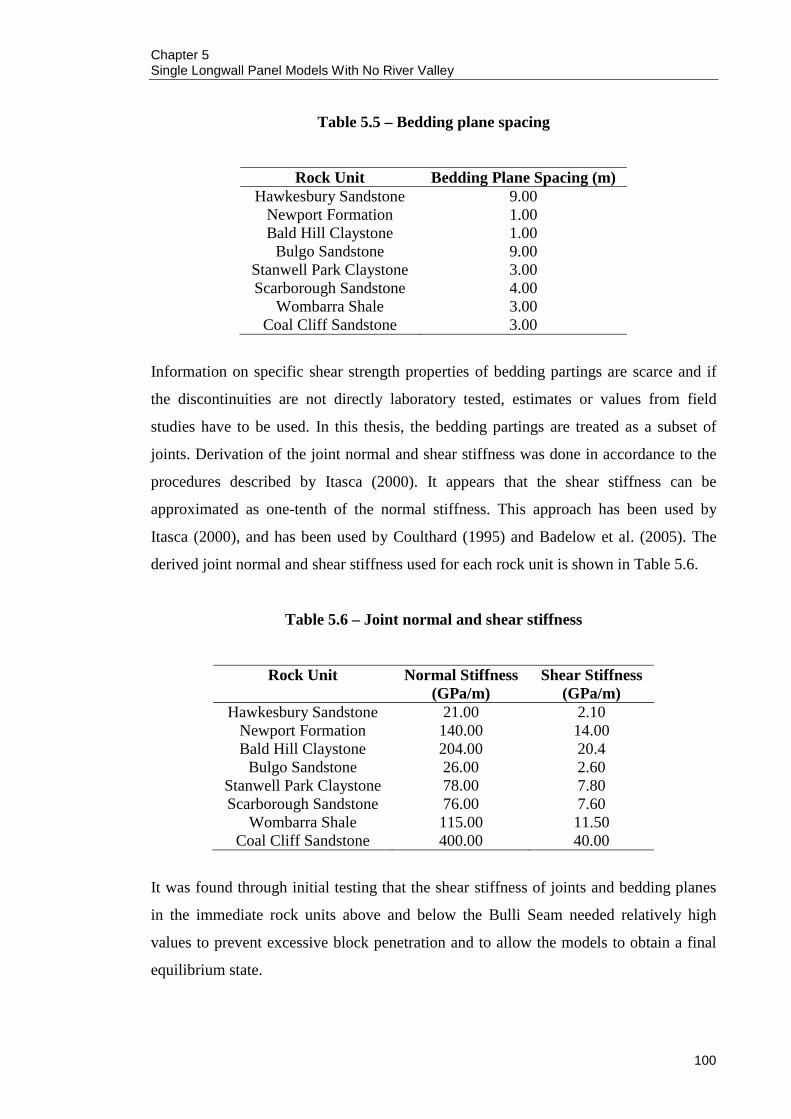
Chapter 5 Single Longwall Panel Models With No River Valley
100
Table 5.5 – Bedding plane spacing
Rock Unit Bedding Plane Spacing (m) Hawkesbury Sandstone 9.00
Newport Formation 1.00 Bald Hill Claystone 1.00
Bulgo Sandstone 9.00 Stanwell Park Claystone 3.00 Scarborough Sandstone 4.00
Wombarra Shale 3.00 Coal Cliff Sandstone 3.00
Information on specific shear strength properties of bedding partings are scarce and if
the discontinuities are not directly laboratory tested, estimates or values from field
studies have to be used. In this thesis, the bedding partings are treated as a subset of
joints. Derivation of the joint normal and shear stiffness was done in accordance to the
procedures described by Itasca (2000). It appears that the shear stiffness can be
approximated as one-tenth of the normal stiffness. This approach has been used by
Itasca (2000), and has been used by Coulthard (1995) and Badelow et al. (2005). The
derived joint normal and shear stiffness used for each rock unit is shown in Table 5.6.
Table 5.6 – Joint normal and shear stiffness
Rock Unit Normal Stiffness (GPa/m)
Shear Stiffness (GPa/m)
Hawkesbury Sandstone 21.00 2.10 Newport Formation 140.00 14.00 Bald Hill Claystone 204.00 20.4
Bulgo Sandstone 26.00 2.60 Stanwell Park Claystone 78.00 7.80 Scarborough Sandstone 76.00 7.60
Wombarra Shale 115.00 11.50 Coal Cliff Sandstone 400.00 40.00
It was found through initial testing that the shear stiffness of joints and bedding planes
in the immediate rock units above and below the Bulli Seam needed relatively high
values to prevent excessive block penetration and to allow the models to obtain a final
equilibrium state.
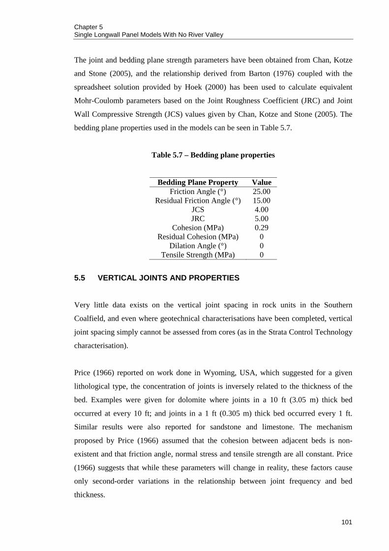
Chapter 5 Single Longwall Panel Models With No River Valley
101
The joint and bedding plane strength parameters have been obtained from Chan, Kotze
and Stone (2005), and the relationship derived from Barton (1976) coupled with the
spreadsheet solution provided by Hoek (2000) has been used to calculate equivalent
Mohr-Coulomb parameters based on the Joint Roughness Coefficient (JRC) and Joint
Wall Compressive Strength (JCS) values given by Chan, Kotze and Stone (2005). The
bedding plane properties used in the models can be seen in Table 5.7.
Table 5.7 – Bedding plane properties
Bedding Plane Property Value Friction Angle (°) 25.00
Residual Friction Angle (°) 15.00 JCS 4.00 JRC 5.00
Cohesion (MPa) 0.29 Residual Cohesion (MPa) 0
Dilation Angle (°) 0 Tensile Strength (MPa) 0
5.5 VERTICAL JOINTS AND PROPERTIES
Very little data exists on the vertical joint spacing in rock units in the Southern
Coalfield, and even where geotechnical characterisations have been completed, vertical
joint spacing simply cannot be assessed from cores (as in the Strata Control Technology
characterisation).
Price (1966) reported on work done in Wyoming, USA, which suggested for a given
lithological type, the concentration of joints is inversely related to the thickness of the
bed. Examples were given for dolomite where joints in a 10 ft (3.05 m) thick bed
occurred at every 10 ft; and joints in a 1 ft (0.305 m) thick bed occurred every 1 ft.
Similar results were also reported for sandstone and limestone. The mechanism
proposed by Price (1966) assumed that the cohesion between adjacent beds is non-
existent and that friction angle, normal stress and tensile strength are all constant. Price
(1966) suggests that while these parameters will change in reality, these factors cause
only second-order variations in the relationship between joint frequency and bed
thickness.
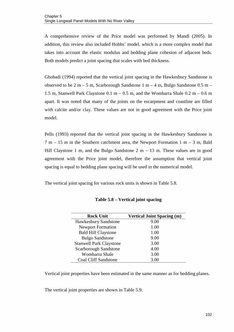
Chapter 5 Single Longwall Panel Models With No River Valley
102
A comprehensive review of the Price model was performed by Mandl (2005). In
addition, this review also included Hobbs’ model, which is a more complex model that
takes into account the elastic modulus and bedding plane cohesion of adjacent beds.
Both models predict a joint spacing that scales with bed thickness.
Ghobadi (1994) reported that the vertical joint spacing in the Hawkesbury Sandstone is
observed to be 2 m – 5 m, Scarborough Sandstone 1 m – 4 m, Bulgo Sandstone 0.5 m –
1.5 m, Stanwell Park Claystone 0.1 m – 0.5 m, and the Wombarra Shale 0.2 m – 0.6 m
apart. It was noted that many of the joints on the escarpment and coastline are filled
with calcite and/or clay. These values are not in good agreement with the Price joint
model.
Pells (1993) reported that the vertical joint spacing in the Hawkesbury Sandstone is
7 m – 15 m in the Southern catchment area, the Newport Formation 1 m – 3 m, Bald
Hill Claystone 1 m, and the Bulgo Sandstone 2 m – 13 m. These values are in good
agreement with the Price joint model, therefore the assumption that vertical joint
spacing is equal to bedding plane spacing will be used in the numerical model.
The vertical joint spacing for various rock units is shown in Table 5.8.
Table 5.8 – Vertical joint spacing
Rock Unit Vertical Joint Spacing (m) Hawkesbury Sandstone 9.00
Newport Formation 1.00 Bald Hill Claystone 1.00
Bulgo Sandstone 9.00 Stanwell Park Claystone 3.00 Scarborough Sandstone 4.00
Wombarra Shale 3.00 Coal Cliff Sandstone 3.00
Vertical joint properties have been estimated in the same manner as for bedding planes.
The vertical joint properties are shown in Table 5.9.

Chapter 5 Single Longwall Panel Models With No River Valley
103
Table 5.9 – Vertical joint properties
Property Vertical Joint Friction Angle (°) 19.00
Residual Friction Angle (°) 15.00 JCS 2.00 JRC 8.00
Cohesion (MPa) 0.86 Residual Cohesion (MPa) 0
Dilation Angle (°) 0 Tensile Strength (MPa) 0
For simplicity, vertical joint dip was assumed to be 90°, forming perfectly square blocks
(as vertical joint spacing is assumed to be equal to bedding plane spacing). Coulthard
(1995) noticed that vertical joint dip played an important role in the caving and bulking
of the goaf but ultimately could not produce the required bulking factor.
5.6 IN-SITU STRESS
A thorough review of regional and local in-situ stress has been compiled by the CSIRO
for their numerical modelling (CSIRO Petroleum 2002). From 206 measurements across
the entire Sydney Basin, the ratio of horizontal stress to vertical stress was found to be
in the range of 1.5 – 2.0. Table 5.10 shows the horizontal to vertical stress ratio for the
Appin, Westcliff and Tower collieries, measured adjacent to the Cataract – Nepean
River gorges.
Table 5.10 – Horizontal to vertical stress ratios (after CSIRO Petroleum 2002)
Colliery σH/σV Appin 1.75
West Cliff 1.40 Tower 3.26
The average of the horizontal to vertical stress ratios in Table 5.10 is approximately
two, and in the Southern Coalfield, the horizontal stress is usually considered to be
twice the vertical stress so for the numerical models, a horizontal to vertical stress ratio
of two was implemented.

Chapter 5 Single Longwall Panel Models With No River Valley
104
5.7 MESH GENERATION
The mesh employed was relatively simple. Each block was subdivided into four
constant strain zones. It was noted by Coulthard (1995) that this may result in a unit of
large blocks being excessively stiffer than a unit of smaller blocks. If this occurs in the
models, the mesh density will be increased in the areas of interest. A typical
representation of the mesh can be seen in Figure 5.1.

Chapter 5 Single Longwall Panel Models With No River Valley
105
Fig. 5.1 – Typical mesh configuration for all models
Bul
go S
ands
tone
Stan
wel
l Par
k C
lays
tone
Scar
boro
ugh
Sand
ston
e
Wom
barr
a Sh
ale
Coa
l Clif
f San
dsto
ne
Bul
li Se
am
Chapter 5 Single Longwall Panel Models With No River Valley
106
5.8 CONSTITUTIVE MODELS
The constitutive model employed for the rock blocks was the standard Mohr-Coulomb
model. The constitutive model used for the joints was the Coulomb slip with residual
strength model. This model simulates displacement weakening of the joint by the loss of
frictional, cohesive and/or tensile strength at the onset of shear or tensile failure (Itasca
2000). This model is suitable for general rock mechanics, including underground
excavations. The definition of a discontinuity means that the tensile strength is suitable
to be set to zero.
5.9 BOUNDARY CONDITIONS
The models were constrained in the x-direction on the sides of the models, and the
bottoms of the models were constrained in the y-direction. The top of each model,
representing the ground surface was left as a free surface.
5.10 HISTORIES
History points were placed along the surface at a distance determined by the vertical
joint spacing of the Hawkesbury Sandstone (9 m). The history points on the surface
monitored movements in the x and y-directions in order to enable the calculation of
vertical subsidence (and goaf edge subsidence), strain and tilt.
5.11 MODEL GEOMETRY AND INITIAL TEST MODELS
The data from which Holla and Barclay (2000) derived their single longwall panel, Bulli
Seam subsidence curves has been reproduced in Table 5.11. The data that was derived
from pillar extraction and Wongawilli Seam extraction will be excluded from the
modelling. It is noted that the extraction details are approximate figures only.
Figure 5.2 is a graphical representation of the thickness of the stratigraphic units in the
overburden, grouped according to colliery. As the extraction details in Table 5.11 are
approximate figures, a reconciliation of the Bulli seam depth (Figure 5.2) and the cover
depth (Table 5.11) produced expected errors, in some cases considerable. As Figure 5.2

Chapter 5 Single Longwall Panel Models With No River Valley
107
is the closest approximation of stratigraphic unit thickness for several collieries, it was
used for the derivation of the thickness of rock units above the Bulli seam for different
mines. The longwall panel widths were derived from Table 5.11 and combined with the
information from Figure 5.2 to produce the number of models required.
Excluding mines that utilise pillar extraction, extract the Wongawilli Seam, and whose
stratigraphic details do not appear in Figure 5.2, it was concluded that four models can
be created from the available data (Table 5.12). Unfortunately, some stratigraphic
details were missing for Appin, Tower and South Bulli collieries. It was decided to
exclude these mines from the models to reduce uncertainty that would be introduced by
estimating the thickness of the missing units. It must be noted that whilst 18 potential
models can be created with the available data, four models was considered sufficient to
cover the range of W/H ratios represented in the single longwall panel subsidence curve
in Holla and Barclay (2000).
Symmetry was utilised to halve the size of the models and run times needed. The plane
of symmetry is on the right hand side of the models as can be seen in Figures 5.3 to 5.6.
To determine the width of each model, a boundary was placed at an arbitrary distance
from the edge of the longwall panel and the model was cycled using the auto damp
option to ensure quick solution times. The location of the boundary was then adjusted so
a full subsidence profile could be produced. A comparison between the subsidence
profile produced by the default local damping, the optional auto damping and local
damping combined with a sub-elastic stage (sets joints and zone constitutive models to
infinite strength for initial equilibrium cycling) was made for Model 4 and the resulting
subsidence profiles can be seen in Figure 5.7.
The auto damping option produced maximum subsidence of 479 mm, whilst the default
local damping produced a maximum subsidence of 476 mm. The sub-elastic stage with
local damping produced 475 mm of subsidence. The difference in maximum developed
subsidence between the highest value (auto damping) and the lowest value (sub-elastic
with local damping) was 4 mm or 0.84 %, therefore auto damping was deemed suitable
for use with the final models. Model run times with auto damping are significantly
lower as well, 7.5 hours compared to eight days with local damping.

Chapter 5 Single Longwall Panel Models With No River Valley
108
Model depth was dependant on stratigraphy and the stratigraphic sequence (in
descending order) for the models was as follows:
Hawkesbury Sandstone,
Newport Formation,
Bald Hill Claystone,
Bulgo Sandstone,
Stanwell Park Claystone,
Scarborough Sandstone,
Wombarra Shale,
Coal Cliff Sandstone,
Bulli Seam,
Loddon Sandstone,
Balgownie Seam,
Lawrence Sandstone,
Cape Horn Seam,
UN2,
Hargraves Coal Member,
UN3,
Wongawilli Seam, and
Kembla Sandstone.
Where UN2 and UN3 stand for Un-Named members 1 and 2 respectively.
The stratigraphic sequence below the Bulli Seam has been derived from the
geotechnical characterisation performed by MacGregor and Conquest (2005) and will
be used for all models.
Table 5.13 contains the thickness of stratigraphic units according to the models listed in
Table 5.12.
Table 5.14 contains the finalised width and depth for each UDEC model (designated
Model 1, Model 2, Model 3 and Model 4).

Chapter 5 Single Longwall Panel Models With No River Valley
109
Table 5.11 – Details for various mines used in the derivation of the empirical
subsidence prediction curves (Holla & Barclay 2000)
Colliery Panel Individual Panel
Width (m) Cover Depth
(m) Extracted
Thickness (m) Appin LWs 1 & 2 150-170 490 2.70
LWs 5-9 145-150 500 2.80 LWs 14-18 207 500 2.70 LWs 21-29 207 490 2.50
Bellambi West LWs 501-506 110 320 2.50 Bulli SW 1 & 2* 79-86 300 2.30
Coal Cliff 221-224, & 260*** 96-920 460 2.60 Cordeaux LWs 17-23A 158 450 2.50 Elouera LW 1 160 330 3.00 Kemira LWs 4-6 160-189 190-235 2.70
Metropolitan SW 1** 105-336 470 2.70 Oakdale LW 5 160 360-410 2.20
South Bulli 200 series LWs 145 440 2.50 300 series LWs 145 450 2.50 LWs K to N 145 445-465 2.65 LWs 9-11 145 400 2.65
Tahmoor 201* 260 430 1.90 LWs 3-9 190 415-425 2.10
Tower LWs 1-3 110 485 2.60 LWs 6-8 155 480 2.60
West Cliff LW 1 145 470 2.65 421* 118 455 2.65 LWs 16-21 205 470-480 2.60
Note 1 – Width refers to the width of individual panels Note 2 – Values of width, cover depth and extracted seam thickness are approximate * indicates pillar extraction; ** indicates short walls; *** indicates Wongawilli type Note 3 – The seam extracted was the Bulli seam in all cases except in Elouera and Kemira Collieries where it was the Wongawilli Seam
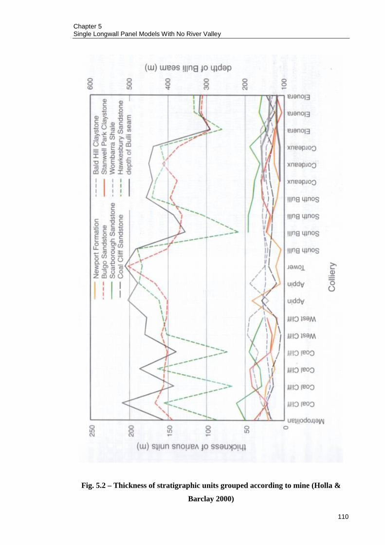
Chapter 5 Single Longwall Panel Models With No River Valley
110
Fig. 5.2 – Thickness of stratigraphic units grouped according to mine (Holla &
Barclay 2000)
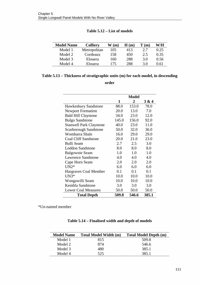
Chapter 5 Single Longwall Panel Models With No River Valley
111
Table 5.12 – List of models
Model Name Colliery W (m) H (m) T (m) W/H Model 1 Metropolitan 105 413 2.7 0.25 Model 2 Cordeaux 158 450 2.5 0.35 Model 3 Elouera 160 288 3.0 0.56 Model 4 Elouera 175 288 3.0 0.61
Table 5.13 – Thickness of stratigraphic units (m) for each model, in descending
order
Model 1 2 3 & 4
Hawkesbury Sandstone 88.0 153.0 78.0 Newport Formation 20.0 13.0 7.0 Bald Hill Claystone 34.0 23.0 12.0 Bulgo Sandstone 145.0 156.0 92.0 Stanwell Park Claystone 40.0 23.0 11.0 Scarborough Sandstone 50.0 32.0 36.0 Wombarra Shale 16.0 29.0 29.0 Coal Cliff Sandstone 20.0 21.0 23.0 Bulli Seam 2.7 2.5 3.0 Loddon Sandstone 8.0 8.0 8.0 Balgownie Seam 1.0 1.0 1.0 Lawrence Sandstone 4.0 4.0 4.0 Cape Horn Seam 2.0 2.0 2.0 UN2* 6.0 6.0 6.0 Hargraves Coal Member 0.1 0.1 0.1 UN3* 10.0 10.0 10.0 Wongawilli Seam 10.0 10.0 10.0 Kembla Sandstone 3.0 3.0 3.0 Lower Coal Measures 50.0 50.0 50.0
Total Depth 509.8 546.6 385.1
*Un-named member
Table 5.14 – Finalised width and depth of models
Model Name Total Model Width (m) Total Model Depth (m) Model 1 815 509.8 Model 2 874 546.6 Model 3 480 385.1 Model 4 525 385.1

Chapter 5 Single Longwall Panel Models With No River Valley
112
Fig. 5.3 – Model 1 geometry
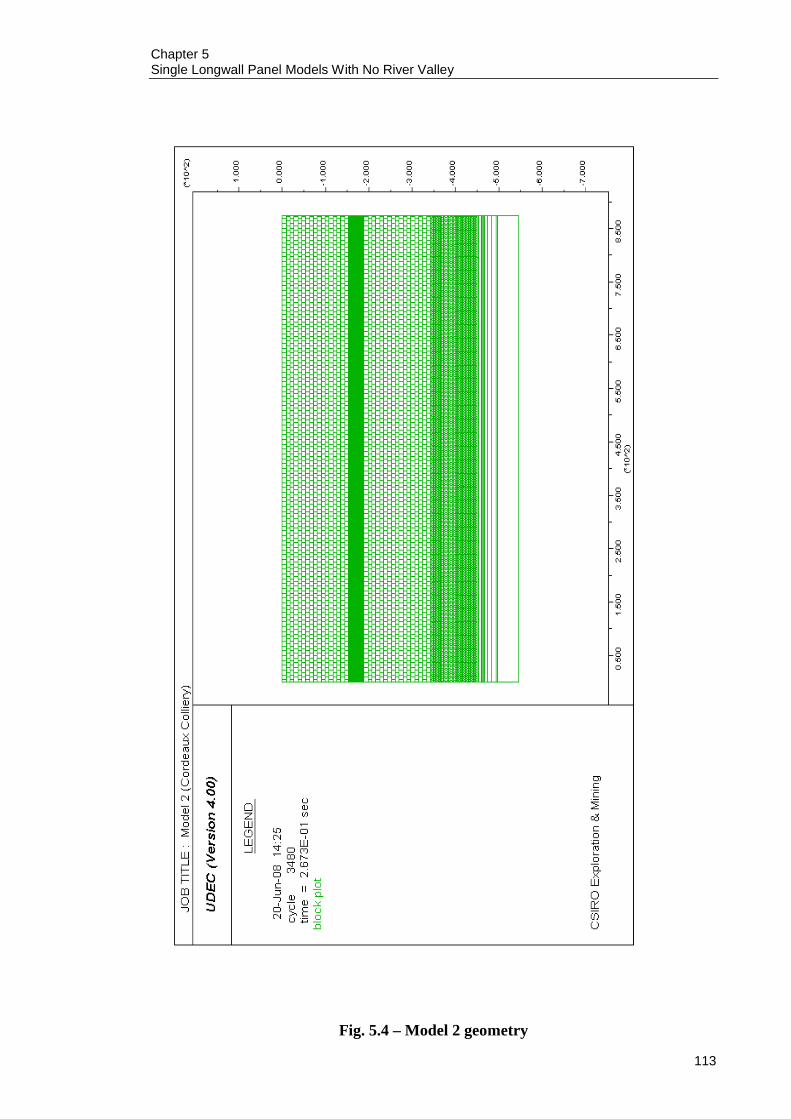
Chapter 5 Single Longwall Panel Models With No River Valley
113
Fig. 5.4 – Model 2 geometry
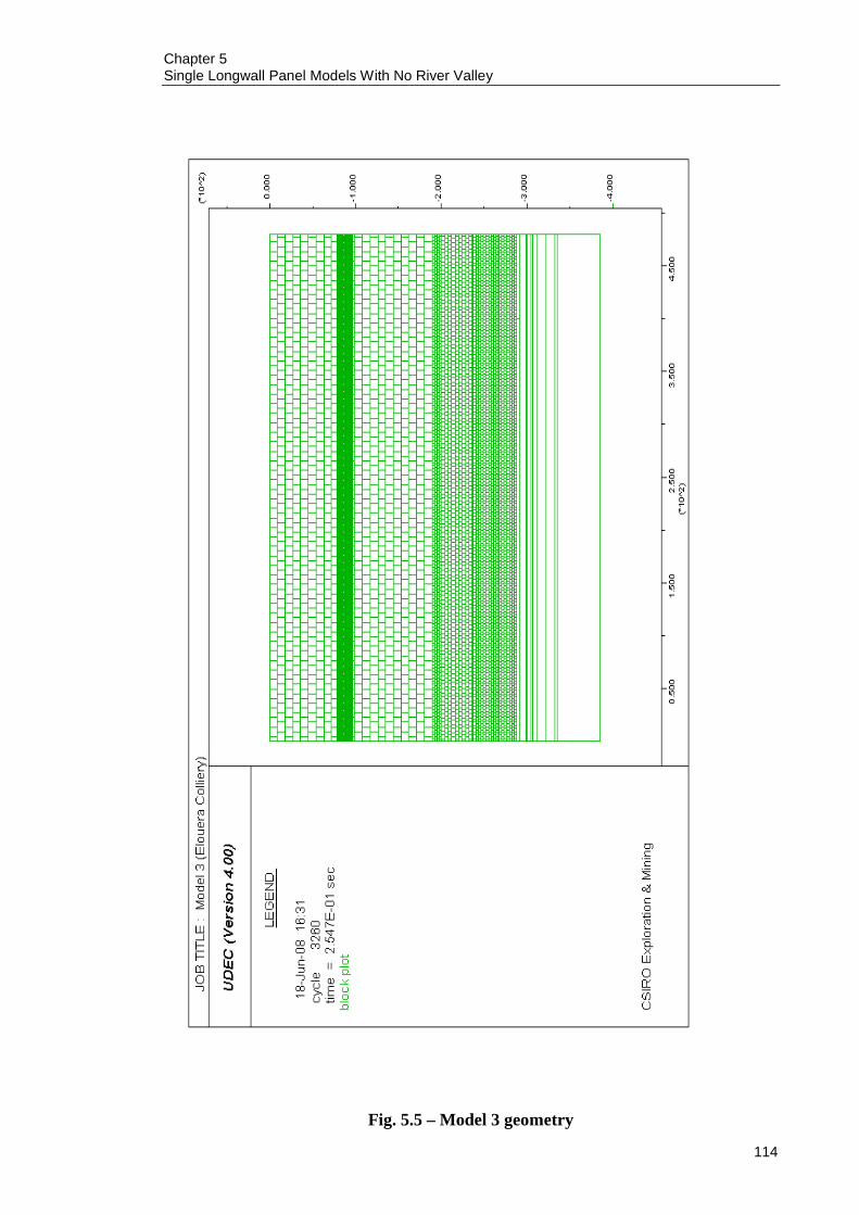
Chapter 5 Single Longwall Panel Models With No River Valley
114
Fig. 5.5 – Model 3 geometry

Chapter 5 Single Longwall Panel Models With No River Valley
115
Fig. 5.6– Model 4 geometry

Chapter 5 Single Longwall Panel Models With No River Valley
116
Fig. 5.7 – Subsidence profiles for different damping options
-550
-450
-350
-250
-150-50
010
020
030
040
050
0
Subsidence (mm)
X P
ositi
on (m
)
Mod
el 4
Initi
al T
estin
g
Aut
o da
mpi
ng
Loca
l da
mpi
ng
Ela
stic
sub
st
age,
loca
l da
mpi
ng

Chapter 5 Single Longwall Panel Models With No River Valley
117
5.12 RESULTS
The details of the single longwall panel flat terrain models can be found in Tables 5.12,
5.13 and 5.14. The results from the four models are presented in Table 5.15.
Table 5.15 – Results from single longwall panel flat terrain models
Parameter Model 1 Model 2 Model 3 Model 4 W/H 0.25 0.35 0.56 0.61 T (m) 2.70 2.50 3.00 3.00
Smax (mm) 39 163 328 479 Sgoaf (mm) 38 91 89 110
+ Emax (mm/m) 0.04 0.07 0.75 1.55 - Emax (mm/m) 0.23 0.33 0.58 0.69 Gmax (mm/m) 0.11 1.13 3.92 5.64
Rmin (km) 81.62 61.98 17.46 8.45 D (m) -173.00 -205.50 18.50 26.02 Smax/T 0.01 0.07 0.11 0.16
Sgoaf/Smax 0.97 0.56 0.27 0.23 K1 0.42 0.19 0.66 0.93 K2 2.41 0.91 0.51 0.42 K3 1.15 3.11 3.44 3.39
D/H -0.42 -0.46 0.06 0.09
Where,
W = Width of longwall panel
H = Depth of cover
T = Extracted seam thickness
Smax = Maximum developed subsidence over centre of longwall
Sgoaf = Maximum developed subsidence over goaf edge
Emax = Maximum developed strain (+ve tensile, -ve compressive)
Gmax = Maximum developed tilt
Rmin = Radius of curvature
D = Distance of inflection point relative to goaf edge (negative values
outside goaf, positive values inside goaf)
K1 = Tensile strain factor
K2 = Compressive strain factor
K3 = Tilt factor

Chapter 5 Single Longwall Panel Models With No River Valley
118
To put the results into perspective, the results from Table 5.15 are superimposed onto
the corresponding empirical curves from Holla and Barclay (2000). These are shown in
Figures 5.8 (subsidence factor), 5.9 (goaf edge subsidence factor), 5.10 (tensile strain
factor), 5.11 (compressive strain factor), 5.12 (tilt factor) and 5.13 (location of inflection
point).

Chapter 5 Single Longwall Panel Models With No River Valley
119
Fig. 5.8 – Superimposed model results for Smax/T (after Holla & Barclay 2000)

Chapter 5 Single Longwall Panel Models With No River Valley
120
Fig. 5.9 – Superimposed model results for Sgoaf/Smax (after Holla & Barclay 2000)

Chapter 5 Single Longwall Panel Models With No River Valley
121
Fig. 5.10 – Superimposed model results for K1 (after Holla & Barclay 2000)

Chapter 5 Single Longwall Panel Models With No River Valley
122
Fig. 5.11 – Superimposed model results for K2 (after Holla & Barclay 2000)

Chapter 5 Single Longwall Panel Models With No River Valley
123
Fig. 5.12 – Superimposed model results for K3 (after Holla & Barclay 2000)

Chapter 5 Single Longwall Panel Models With No River Valley
124
Fig. 5.13 – Superimposed model results for D/H (after Holla & Barclay 2000)
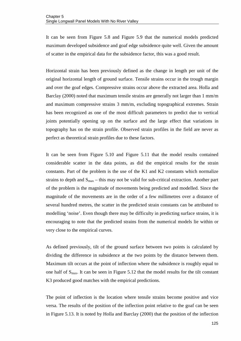
Chapter 5 Single Longwall Panel Models With No River Valley
125
It can be seen from Figure 5.8 and Figure 5.9 that the numerical models predicted
maximum developed subsidence and goaf edge subsidence quite well. Given the amount
of scatter in the empirical data for the subsidence factor, this was a good result.
Horizontal strain has been previously defined as the change in length per unit of the
original horizontal length of ground surface. Tensile strains occur in the trough margin
and over the goaf edges. Compressive strains occur above the extracted area. Holla and
Barclay (2000) noted that maximum tensile strains are generally not larger than 1 mm/m
and maximum compressive strains 3 mm/m, excluding topographical extremes. Strain
has been recognized as one of the most difficult parameters to predict due to vertical
joints potentially opening up on the surface and the large effect that variations in
topography has on the strain profile. Observed strain profiles in the field are never as
perfect as theoretical strain profiles due to these factors.
It can be seen from Figure 5.10 and Figure 5.11 that the model results contained
considerable scatter in the data points, as did the empirical results for the strain
constants. Part of the problem is the use of the K1 and K2 constants which normalize
strains to depth and Smax – this may not be valid for sub-critical extraction. Another part
of the problem is the magnitude of movements being predicted and modelled. Since the
magnitude of the movements are in the order of a few millimetres over a distance of
several hundred metres, the scatter in the predicted strain constants can be attributed to
modelling ‘noise’. Even though there may be difficulty in predicting surface strains, it is
encouraging to note that the predicted strains from the numerical models lie within or
very close to the empirical curves.
As defined previously, tilt of the ground surface between two points is calculated by
dividing the difference in subsidence at the two points by the distance between them.
Maximum tilt occurs at the point of inflection where the subsidence is roughly equal to
one half of Smax. It can be seen in Figure 5.12 that the model results for the tilt constant
K3 produced good matches with the empirical predictions.
The point of inflection is the location where tensile strains become positive and vice
versa. The results of the position of the inflection point relative to the goaf can be seen
in Figure 5.13. It is noted by Holla and Barclay (2000) that the position of the inflection

Chapter 5 Single Longwall Panel Models With No River Valley
126
point falls inside the goaf for W/H ratios greater than 0.5 or outside the goaf for W/H
ratios less than 0.5. It can be seen that this observation holds true for Model 1 (W/H =
0.25), Model 3 (W/H = 0.56) and Model 4 (W/H = 0.61), and the predicted location of
the inflection point falls within the range of empirical data scatter. The predicted
subsidence at the inflection point was roughly one half of predicted Smax for all models
and this is in agreement with Holla and Barclay (2000).
The calculated angle of draw for the models varied between 18° and 41°. This produced
an average value of 29°. The angle of draw was calculated using the 20 mm cut-off
limit. The average angle of draw from Holla and Barclay (2000) is also 29°. This was an
exact match but it must also be noted that there seems to be no apparent relationship
between angle of draw and W/H ratio, the predicted values can only be compared to the
empirical values and not be verified in any way.
The UDEC subsidence development history above the centre of the longwall panel,
subsidence profile, strain profile, tilt profile, yielded zones and caving development, and
joint slip for all four models are shown in Figures 5.14 to 5.41.
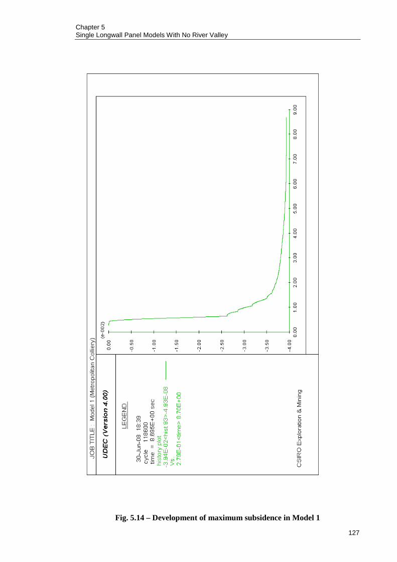
Chapter 5 Single Longwall Panel Models With No River Valley
127
Fig. 5.14 – Development of maximum subsidence in Model 1

Chapter 5 Single Longwall Panel Models With No River Valley
128
Fig. 5.15 – Subsidence profile for Model 1
-45.
00
-40.
00
-35.
00
-30.
00
-25.
00
-20.
00
-15.
00
-10.
00
-5.0
0
0.00
0.00
100.
0020
0.00
300.
0040
0.00
500.
0060
0.00
700.
0080
0.00
Subsidence (mm)
X P
ositi
on (m
)
Mod
el 1
Sub
side
nce
Pro
file

Chapter 5 Single Longwall Panel Models With No River Valley
129
Fig. 5.16 – Strain profile for Model 1
-0.1
1
-0.0
9
-0.0
7
-0.0
5
-0.0
3
-0.0
1
0.01
0.03
0.05
0.00
100.
0020
0.00
300.
0040
0.00
500.
0060
0.00
700.
0080
0.00
Strain (mm/m)
X P
ositi
on (m
)
Mod
el 1
Str
ain
Pro
file

Chapter 5 Single Longwall Panel Models With No River Valley
130
Fig. 5.17 – Tilt profile for Model 1
-0.1
5
-0.1
3
-0.1
1
-0.0
9
-0.0
7
-0.0
5
-0.0
3
-0.0
10.00
100.
0020
0.00
300.
0040
0.00
500.
0060
0.00
700.
0080
0.00
Tilt (mm/m)
X P
ositi
on (m
)
Mod
el 1
Tilt
Pro
file

Chapter 5 Single Longwall Panel Models With No River Valley
131
Fig. 5.18 – Yielded zones and caving development in Model 1

Chapter 5 Single Longwall Panel Models With No River Valley
132
Fig. 5.19 – Detailed view of yielded zones in Model 1
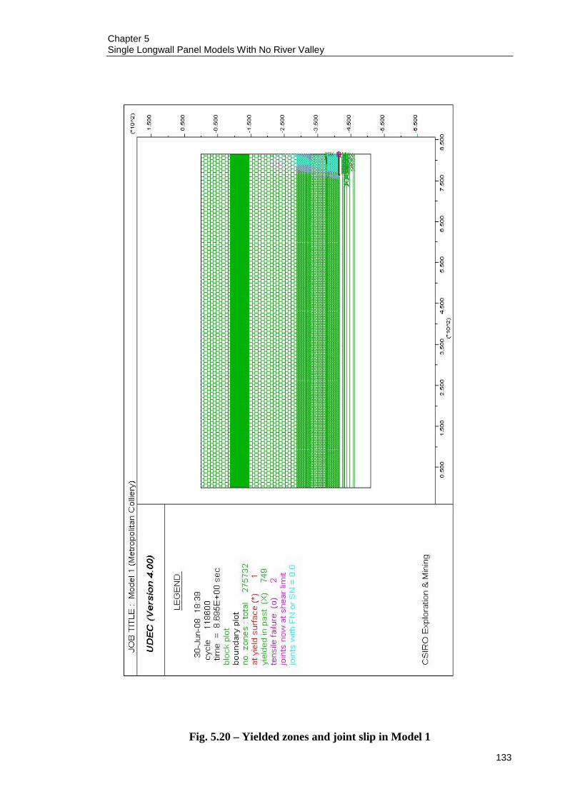
Chapter 5 Single Longwall Panel Models With No River Valley
133
Fig. 5.20 – Yielded zones and joint slip in Model 1

Chapter 5 Single Longwall Panel Models With No River Valley
134
Fig. 5.21 - Development of maximum subsidence in Model 2
Chapter 5 Single Longwall Panel Models With No River Valley
135
Fig. 5.22 – Subsidence profile for Model 2
-180
.00
-160
.00
-140
.00
-120
.00
-100
.00
-80.
00
-60.
00
-40.
00
-20.
00
0.00
0.00
100.
0020
0.00
300.
0040
0.00
500.
0060
0.00
700.
0080
0.00
Subsidence (mm)
X P
ositi
on (m
)
Mod
el 2
Sub
side
nce
Pro
file

Chapter 5 Single Longwall Panel Models With No River Valley
136
Fig. 5.23 – Strain profile for Model 2
-0.3
5
-0.3
-0.2
5
-0.2
-0.1
5
-0.1
-0.0
50
0.050.1 0.
0010
0.00
200.
0030
0.00
400.
0050
0.00
600.
0070
0.00
800.
00
Strain (mm/m)
X P
ositi
on (m
)
Mod
el 2
Str
ain
Pro
file

Chapter 5 Single Longwall Panel Models With No River Valley
137
Fig. 5.24 – Tilt profile for Model 2
-1.4
0
-1.2
0
-1.0
0
-0.8
0
-0.6
0
-0.4
0
-0.2
0
0.00
0.00
100.
0020
0.00
300.
0040
0.00
500.
0060
0.00
700.
0080
0.00
Tilt (mm/m)
X P
ositi
on (m
)
Mod
el 2
Tilt
Pro
file

Chapter 5 Single Longwall Panel Models With No River Valley
138
Fig. 5.25 – Yielded zones and caving development in Model 2
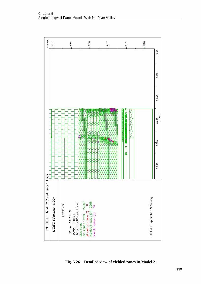
Chapter 5 Single Longwall Panel Models With No River Valley
139
Fig. 5.26 – Detailed view of yielded zones in Model 2
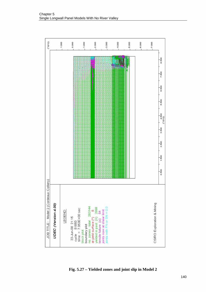
Chapter 5 Single Longwall Panel Models With No River Valley
140
Fig. 5.27 – Yielded zones and joint slip in Model 2

Chapter 5 Single Longwall Panel Models With No River Valley
141
Fig. 5.28 – Development of maximum subsidence in Model 3

Chapter 5 Single Longwall Panel Models With No River Valley
142
Fig. 5.29 – Subsidence profile for Model 3
-350
.00
-300
.00
-250
.00
-200
.00
-150
.00
-100
.00
-50.
00
0.00
50.0
0 0.00
50.0
010
0.00
150.
0020
0.00
250.
0030
0.00
350.
0040
0.00
450.
00
Subsidence (mm)
X P
ositi
on (m
)
Mod
el 3
Sub
side
nce
Pro
file
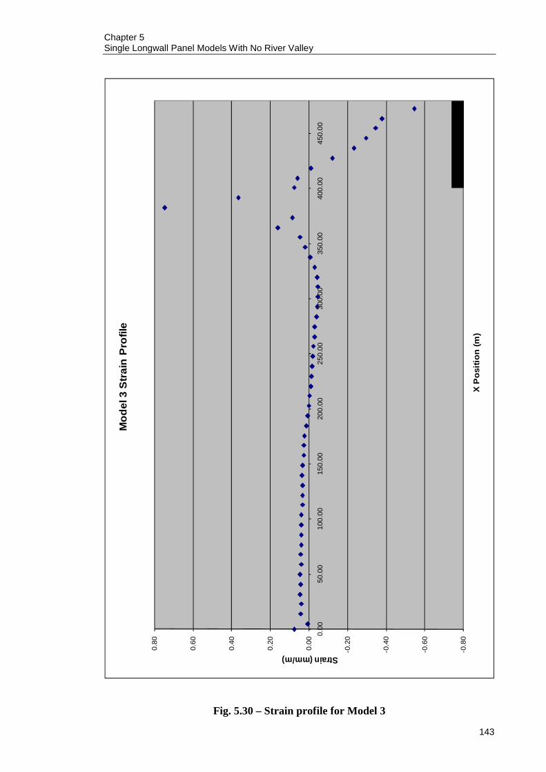
Chapter 5 Single Longwall Panel Models With No River Valley
143
Fig. 5.30 – Strain profile for Model 3
-0.8
0
-0.6
0
-0.4
0
-0.2
0
0.00
0.20
0.40
0.60
0.80
0.00
50.0
010
0.00
150.
0020
0.00
250.
0030
0.00
350.
0040
0.00
450.
00
Strain (mm/m)
X P
ositi
on (m
)
Mod
el 3
Str
ain
Pro
file

Chapter 5 Single Longwall Panel Models With No River Valley
144
Fig. 5.31 – Tilt profile for Model 3
-4.4
0
-3.9
0
-3.4
0
-2.9
0
-2.4
0
-1.9
0
-1.4
0
-0.9
0
-0.4
0
0.10
0.00
50.0
010
0.00
150.
0020
0.00
250.
0030
0.00
350.
0040
0.00
450.
00
Tilt (mm/m)
X P
ositi
on (m
)
Mod
el 3
Tilt
Pro
file
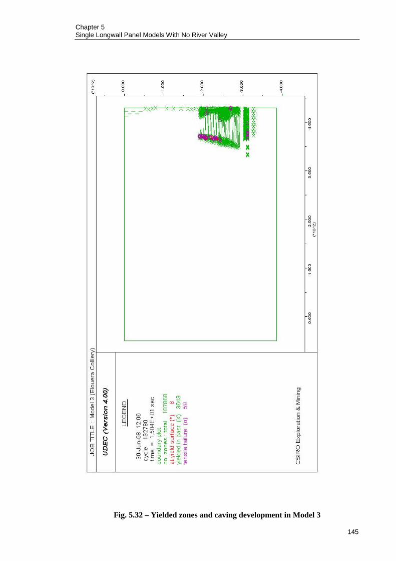
Chapter 5 Single Longwall Panel Models With No River Valley
145
Fig. 5.32 – Yielded zones and caving development in Model 3
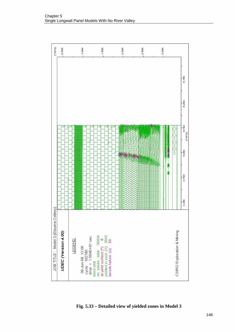
Chapter 5 Single Longwall Panel Models With No River Valley
146
Fig. 5.33 – Detailed view of yielded zones in Model 3

Chapter 5 Single Longwall Panel Models With No River Valley
147
Fig. 5.34 – Yielded zones and joint slip in Model 3
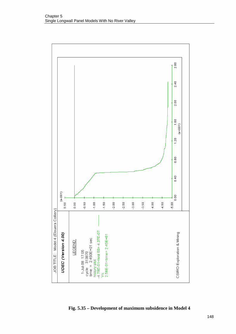
Chapter 5 Single Longwall Panel Models With No River Valley
148
Fig. 5.35 – Development of maximum subsidence in Model 4

Chapter 5 Single Longwall Panel Models With No River Valley
149
Fig. 5.36 – Subsidence profile for Model 4
-550
.00
-500
.00
-450
.00
-400
.00
-350
.00
-300
.00
-250
.00
-200
.00
-150
.00
-100
.00
-50.
00
0.00
50.0
0 0.00
100.
0020
0.00
300.
0040
0.00
500.
00
Subsidence (mm)
X P
ositi
on (m
)
Mod
el 4
Sub
side
nce
Pro
file
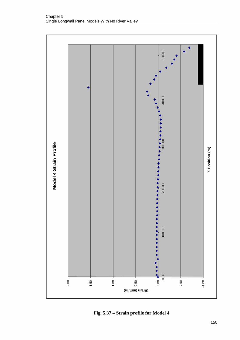
Chapter 5 Single Longwall Panel Models With No River Valley
150
Fig. 5.37 – Strain profile for Model 4
-1.0
0
-0.5
0
0.00
0.50
1.00
1.50
2.00
0.00
100.
0020
0.00
300.
0040
0.00
500.
00
Strain (mm/m)
X P
ositi
on (m
)
Mod
el 4
Str
ain
Pro
file
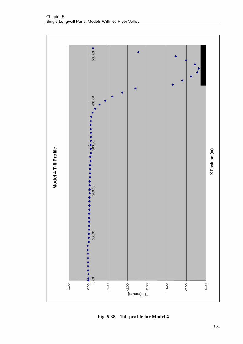
Chapter 5 Single Longwall Panel Models With No River Valley
151
Fig. 5.38 – Tilt profile for Model 4
-6.0
0
-5.0
0
-4.0
0
-3.0
0
-2.0
0
-1.0
0
0.00
1.00
0.00
100.
0020
0.00
300.
0040
0.00
500.
00
Tilt (mm/m)
X P
ositi
on (m
)
Mod
el 4
Tilt
Pro
file

Chapter 5 Single Longwall Panel Models With No River Valley
152
Fig. 5.39– Yielded zones and caving development in Model 4

Chapter 5 Single Longwall Panel Models With No River Valley
153
Fig. 5.40 – Detailed view of yielded zones in Model 4

Chapter 5 Single Longwall Panel Models With No River Valley
154
Fig. 5.41 – Yielded zones and joint slip in Model 4

Chapter 5 Single Longwall Panel Models With No River Valley
155
The subsidence development plots (Figures 5.14, 5.21, 5.28 and 5.35) illustrate that the
models had been cycled to equilibrium until the maximum developed subsidence
stabilised and stopped increasing. This model state was paramount as the quality of the
final results would have been compromised if this state was not reached.
It can be seen that the subsidence profiles (Figures 5.15, 5.22, 5.29 and 5.36), strain
profiles (Figures 5.16, 5.23, 5.30 and 5.37) and tilt profiles (Figures 5.17, 5.24, 5.31 and
5.38) are generally in the expected theoretical shape. The subsidence profiles for all
models indicate that the boundaries were at a sufficient distance from the longwall
extractions. The ‘noise’ in the strain profiles for all models was also evident.
It can also be seen from Figures 5.18, 5.25, 5.32 and 5.39 that caving develops with
accordance to the conceptual subsidence model for the Southern Coalfield (Chapter 2).
Except for Model 1 where the longwall panel may have been too narrow to initiate
substantial caving, it can be seen from Figures 5.19, 5.26, 5.33 and 5.40 that the goaf
angle for Model 2 was between 11° to 25°, Model 3 was 14° to 25°, and Model 4 was
13° to 25°. This compared favourably with numerical modelling by CSIRO Exploration
and Mining and Strata Control Technology (1999) of the caving in the Southern
Coalfield that supported a goaf angle value of 12º.
Caving and cracking events are generally contained below the base of the Bulgo
Sandstone. In Models 3 and 4, the cave zone penetrated through the base of the Bulgo
Sandstone which suggested that the Bulgo Sandstone is the major control on subsidence
up to W/H ratios of approximately 0.5 (Chapter 2). Once the Bulgo Sandstone fails, it is
no longer the massive spanning unit that controls subsidence, resulting in a large
increase in the subsidence factor. This trend is evident in the empirical prediction curve
(see Figure 5.8) and was reflected by the subsidence factors of Model 3 and Model 4. It
was also noticed that the caving of the goaf was not really a massive combination of
block yield and rotations, but more a gradual settling and deflection of the roof strata.
This would have resulted in substantially less bulking in the goaf, but does not seem to
be an issue as far as subsidence predictions are concerned. The failure to produce
bulking in the goaf was also noted by Coulthard (1995).

Chapter 5 Single Longwall Panel Models With No River Valley
156
Figures 5.20, 5.27, 5.34 and 5.41 illustrate the yielded zones of each model, combined
with joint slip. It can be seen that as W/H increases, so does the amount of joint slip in
the vertical and horizontal direction. It was noted that joint slip was more prominent in
rock units that had closely spaced joints. This can be seen in Figures 5.27, 5.34 and
5.41, where substantial joint slip is evident in the Newport Formation and Bald Hill
Claystone.
From the results, it can be seen that the numerical models are satisfactorily verified by
the empirical results when it comes to subsidence predictions and the prediction of the
shape of the subsidence trough over single longwall panels.
5.13 SUMMARY
In this chapter, a set of UDEC numerical models was developed to simulate single panel
longwall extractions. The process of creating the models, including the compilation of
material/joint properties and the determination of the geometry for each individual
model was discussed. It was emphasised that all the material/joint properties should be
transparent and fully traceable to minimise the appearance of ‘adjusting’ certain
parameters to fit a predefined outcome.
From the results, it was seen that the numerical models provided quite a good match to
the empirical results, and the caving development evident in the numerical models also
agreed with the caving characteristics discussed in Chapter 2 and supported the theory
that the Bulgo Sandstone is the control on sub-critical subsidence. Overall, it was
concluded that the numerical models were satisfactorily verified by the empirical results
and a major outcome of this modelling was the creation of a tool that can be used for
sensitivity studies to identify the key controlling parameters. The formation of
numerical models that contain a river valley is the subject of the next chapter. These
numerical models will share the basic characteristics as the models discussed in this
chapter.
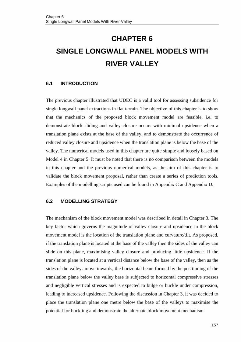
Chapter 6 Single Longwall Panel Models With River Valley
157
CHAPTER 6 SINGLE LONGWALL PANEL MODELS WITH
RIVER VALLEY
6.1 INTRODUCTION
The previous chapter illustrated that UDEC is a valid tool for assessing subsidence for
single longwall panel extractions in flat terrain. The objective of this chapter is to show
that the mechanics of the proposed block movement model are feasible, i.e. to
demonstrate block sliding and valley closure occurs with minimal upsidence when a
translation plane exists at the base of the valley, and to demonstrate the occurrence of
reduced valley closure and upsidence when the translation plane is below the base of the
valley. The numerical models used in this chapter are quite simple and loosely based on
Model 4 in Chapter 5. It must be noted that there is no comparison between the models
in this chapter and the previous numerical models, as the aim of this chapter is to
validate the block movement proposal, rather than create a series of prediction tools.
Examples of the modelling scripts used can be found in Appendix C and Appendix D.
6.2 MODELLING STRATEGY
The mechanism of the block movement model was described in detail in Chapter 3. The
key factor which governs the magnitude of valley closure and upsidence in the block
movement model is the location of the translation plane and curvature/tilt. As proposed,
if the translation plane is located at the base of the valley then the sides of the valley can
slide on this plane, maximising valley closure and producing little upsidence. If the
translation plane is located at a vertical distance below the base of the valley, then as the
sides of the valleys move inwards, the horizontal beam formed by the positioning of the
translation plane below the valley base is subjected to horizontal compressive stresses
and negligible vertical stresses and is expected to bulge or buckle under compression,
leading to increased upsidence. Following the discussion in Chapter 3, it was decided to
place the translation plane one metre below the base of the valleys to maximise the
potential for buckling and demonstrate the alternate block movement mechanism.
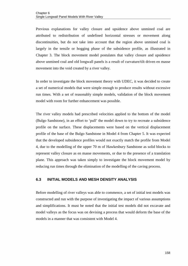
Chapter 6 Single Longwall Panel Models With River Valley
158
Previous explanations for valley closure and upsidence above unmined coal are
attributed to redistribution of undefined horizontal stresses or movement along
discontinuities, but do not take into account that the region above unmined coal is
largely in the tensile or hogging phase of the subsidence profile, as illustrated in
Chapter 3. The block movement model postulates that valley closure and upsidence
above unmined coal and old longwall panels is a result of curvature/tilt driven en masse
movement into the void created by a river valley.
In order to investigate the block movement theory with UDEC, it was decided to create
a set of numerical models that were simple enough to produce results without excessive
run times. With a set of reasonably simple models, validation of the block movement
model with room for further enhancement was possible.
The river valley models had prescribed velocities applied to the bottom of the model
(Bulgo Sandstone), in an effort to ‘pull’ the model down to try to recreate a subsidence
profile on the surface. These displacements were based on the vertical displacement
profile of the base of the Bulgo Sandstone in Model 4 from Chapter 5. It was expected
that the developed subsidence profiles would not exactly match the profile from Model
4, due to the modelling of the upper 70 m of Hawkesbury Sandstone as solid blocks to
represent valley closure as en masse movements, or due to the presence of a translation
plane. This approach was taken simply to investigate the block movement model by
reducing run times through the elimination of the modelling of the caving process.
6.3 INITIAL MODELS AND MESH DENSITY ANALYSIS
Before modelling of river valleys was able to commence, a set of initial test models was
constructed and run with the purpose of investigating the impact of various assumptions
and simplifications. It must be noted that the initial test models did not excavate and
model valleys as the focus was on devising a process that would deform the base of the
models in a manner that was consistent with Model 4.

Chapter 6 Single Longwall Panel Models With River Valley
159
The purpose of the initial modelling was:
To create a methodology that would adequately replicate the vertical
displacements of a chosen rock unit in Model 4 and eliminate the need to model
the caving process,
To investigate the effects of the removal of bedding and joints from the top
70 m of the Hawkesbury Sandstone, and
To ensure that the chosen base of the river valley models did not impact on the
subsequent model results.
The incorporation of these changes meant that it was not necessary to model the caving
process (which was noted in Chapter 5 to be largely contained by the Bulgo Sandstone,
and which also accounted for the majority of running time). The removal of bedding
planes and joints in the top 70 m of the Hawkesbury Sandstone was performed to see if
the observation of rigid body type movement (Holla & Barclay 2000) was present in the
initial models.
In order to determine what rock units could be taken out of the model, the vertical
displacements at the base of the Hawkesbury Sandstone, Newport Formation, Bald Hill
Claystone and Bulgo Sandstone were compared to the vertical displacements at the
surface. A graph of the vertical displacements for the above mentioned units is shown in
Figure 6.1. It can be seen from Figure 6.1 that the vertical displacements at the base of
the Bald Hill Claystone were slightly different to the vertical displacements at the
surface, whilst the vertical displacements at the base of the Bulgo Sandstone were also
slightly different except for those at the centre of the longwall panel. The displacements
noted at the centre of the longwall panel in Figure 6.1 were most likely a result of
bedding planes separating after yield in tension. The Bulgo Sandstone in Model 4
experienced some tensile cracking at its base and was sagging into the caved zone,
hence the large increase in vertical displacement at the centre of the panel. It was
considered making the Bald Hill Claystone the base of the new models, but there was a
chance that any element failure may have encroached the areas of interest hence it was
decided that the Bulgo Sandstone would form the base of the river valley models.

Chapter 6 Single Longwall Panel Models With River Valley
160
In order to replicate the vertical displacements at the base of the Bulgo Sandstone in the
river valley models, a three metre thick beam was incorporated into the base of the
Bulgo Sandstone by creating a bedding plane and assigning very high cohesion, friction
angle and tensile strength to prevent detachment from the base of the Bulgo Sandstone.
This beam had a vertical joint spacing of nine metres so it directly coincided with the
vertical joint spacing of the Hawkesbury Sandstone, from which the vertical
displacements were monitored. These vertical joints were also assigned very high
strength parameters to prevent separation.
According to the UDEC User’s Guide (Itasca 2000), displacements cannot be controlled
directly in UDEC. To deform a boundary to a desired profile, it is necessary to prescribe
the boundary’s velocity for a given number of steps. For example, if the desired
displacement at one point is D, a velocity, V, is applied for a time increment, T (i.e.,
D = VT), where T = ∆tN, ∆t is the timestep and N is the number of steps (or cycles). In
practice, V should be kept small and N large, in order to minimise shocks to the system
being modelled.
The process to pull down the base of the river valley models so the base of the model
matched the base of the Bulgo Sandstone in Model 4 was as follows:
1. Fix the sides of the model and cycle for one step to obtain the time step,
2. Identify grid points at the base of the model to which velocities will be attached,
3. Define the maximum displacement for each previously identified grid point (as
derived from the displacement profile for the Bulgo Sandstone in Model 4),
4. Calculate the y velocity for the identified grid points using V = D/∆tN,
5. Assign y velocities to grid points, and
6. Cycle model for N cycles.
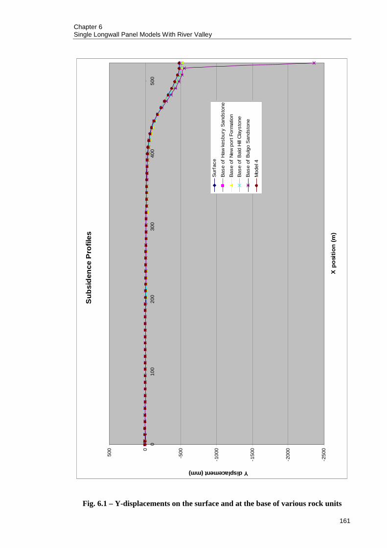
Chapter 6 Single Longwall Panel Models With River Valley
161
Fig. 6.1 – Y-displacements on the surface and at the base of various rock units
Sub
side
nce
Pro
files
-250
0
-200
0
-150
0
-100
0
-5000
500
010
020
030
040
050
0
X p
ositi
on (m
)
Y displacement (mm)
Surf
ace
Base
of H
awke
sbur
y S
ands
tone
Base
of N
ewpo
rt Fo
rmat
ion
Base
of B
ald
Hill
Cla
ysto
ne
Base
of B
ulgo
San
dsto
ne
Mod
el 4

Chapter 6 Single Longwall Panel Models With River Valley
162
To identify the optimum number of steps (N), a series of initial models with the
translation plane at the base of the valley was set up for different values of N (100,
1000, 10000, 20000, 30000, 40000, 50000 and 100000). The vertical displacements at
the base of the Bulgo Sandstone was monitored for each of these models and compared
with Model 4, and the subsidence profile on the surface was also compared to that of
Model 4. Yielded zones were also noted to ensure that the base of the models was at a
sufficient distance below the river valleys.
The geometry of the valleys is a typical representation of valleys in the Southern
Coalfield. The valleys were 70 m deep and 50 m wide (CSIRO Petroleum 2002). For
these simple numerical models, the valleys were assumed to have vertical sides and the
rectangular geometry remained constant, no changes were made to the valley depth,
valley width or slope of the valley sides. The valleys were modelled by creating a
bedding plane at a depth of 70 m in the Hawkesbury Sandstone and creating vertical
joints 50 m apart. The vertical joints were arranged so that the central valley was
situated directly above the longwall centreline. For the models that contained the
translation plane at the base of the valleys, the horizontal joints at the bottom of the
blocks that formed the valleys were assigned the same strength parameters as the
bedding planes in Chapter 5. For the models that contained the translation plane one
metre below the valleys, the translation plane was assigned the same bedding plane
properties as detailed in Chapter 5, whilst the horizontal joints at the base of the valleys
were assigned very high strength parameters to eliminate the effect of those joints. The
remaining material, joint and bedding plane properties remained the same as the models
in Chapter 5, as did the constitutive models and in-situ stress regime (K = 2), in an
effort to maintain consistency. Symmetry was not able to be used because of the
presence of the valley.
The geometry of the initial models can be seen in Figure 6.2. It must be noted that no
valleys were excavated at this stage since the purpose of these models was to determine
the optimum number of cycles required to minimise model run times and provide
consistent results. The width of the initial models was 1050 m and the depth was 189 m.
Figure 6.3 illustrates the mesh (finite different zoning in the blocks) and it can be seen
that it is the same as used in Model 4 (see Figure 5.1) and this has been kept constant in
the initial river valley models only.

Chapter 6 Single Longwall Panel Models With River Valley
163
Fig. 6.2 – Geometry of initial river valley models

Chapter 6 Single Longwall Panel Models With River Valley
164
Fig. 6.3 – Finite different zoning used in valley models

Chapter 6 Single Longwall Panel Models With River Valley
165
The subsidence results from the initial river valley models are summarised in Table 6.1.
Table 6.1 – Subsidence results from initial river valley models
Model Run time (minutes) Maximum subsidence (mm) 100cycles 25 13
1000cycles 30 124 10000cycles 90 196 20000cycles 120 200 30000cycles 150 201 40000cycles 180 201 50000cycles 210 201
100000cycles 420 200
The displacements at the base of the models (base of Bulgo Sandstone) for the models
in Table 6.1 are compared against Model 4 in Figure 6.4. The results from Table 6.1 are
represented in Figure 6.5.
It can be seen from Figure 6.4 that the method of attaching y velocities to required
points and cycling for N steps exactly replicated the required profile. From Figure 6.5, it
can be seen that the resultant subsidence profiles did not match the profile from Model
4, with the maximum developed subsidence in the river valley models 42 % of the
maximum developed subsidence in Model 4. This was expected due to the lack of
bedding and joints in the upper 70 m of the Hawkesbury Sandstone.
It can be seen from Figure 6.5 that the maximum developed subsidence flattened out at
approximately 200 mm. To ensure that any yielded zones did not impact on the area
near the translation plane or the valleys, Figure 6.6 shows the yielded zones for N =
30,000 cycles. It can be seen that the yielded zones were restricted to the base of the
model (in the beam attached to the base) and did not impact on the areas of interest. It
was decided to use N = 30,000 cycles for the subsequent river valley models as it was a
reasonable compromise between maximum developed subsidence (201 mm) and run
time (150 minutes) and the model did not produce unwanted yielding in the areas of
interest.

Chapter 6 Single Longwall Panel Models With River Valley
166
Fig. 6.4 – Vertical displacements at base of Bulgo Sandstone
Ver
tical
Dis
plac
emen
ts a
t Bas
e of
Bul
go S
ands
tone
-250
0
-200
0
-150
0
-100
0
-5000
010
020
030
040
050
0
X P
ositi
on (m
)
Vertical displacements (mm)
Mod
el4
100c
ycle
s
1000
cycl
es
1000
0cyc
les
2000
0cyc
les
3000
0cyc
les
4000
0cyc
les
5000
0cyc
les
1000
00cy
cles
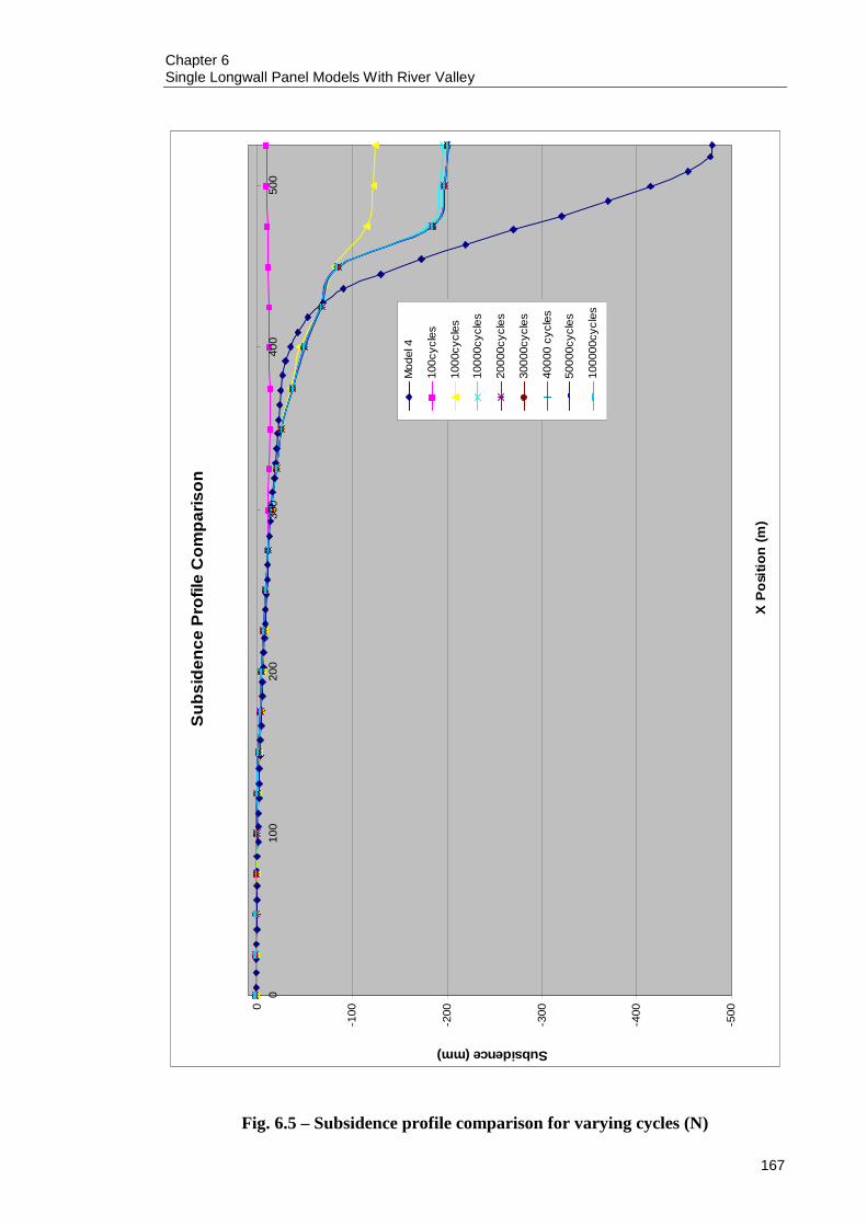
Chapter 6 Single Longwall Panel Models With River Valley
167
Fig. 6.5 – Subsidence profile comparison for varying cycles (N)
Sub
side
nce
Pro
file
Com
paris
on
-500
-400
-300
-200
-1000
010
020
030
040
050
0
X P
ositi
on (m
)
Subsidence (mm)
Mod
el 4
100c
ycle
s
1000
cycl
es
1000
0cyc
les
2000
0cyc
les
3000
0cyc
les
4000
0 cy
cles
5000
0cyc
les
1000
00cy
cles

Chapter 6 Single Longwall Panel Models With River Valley
168
Fig. 6.6 – Yielded zones for N = 30,000 cycles
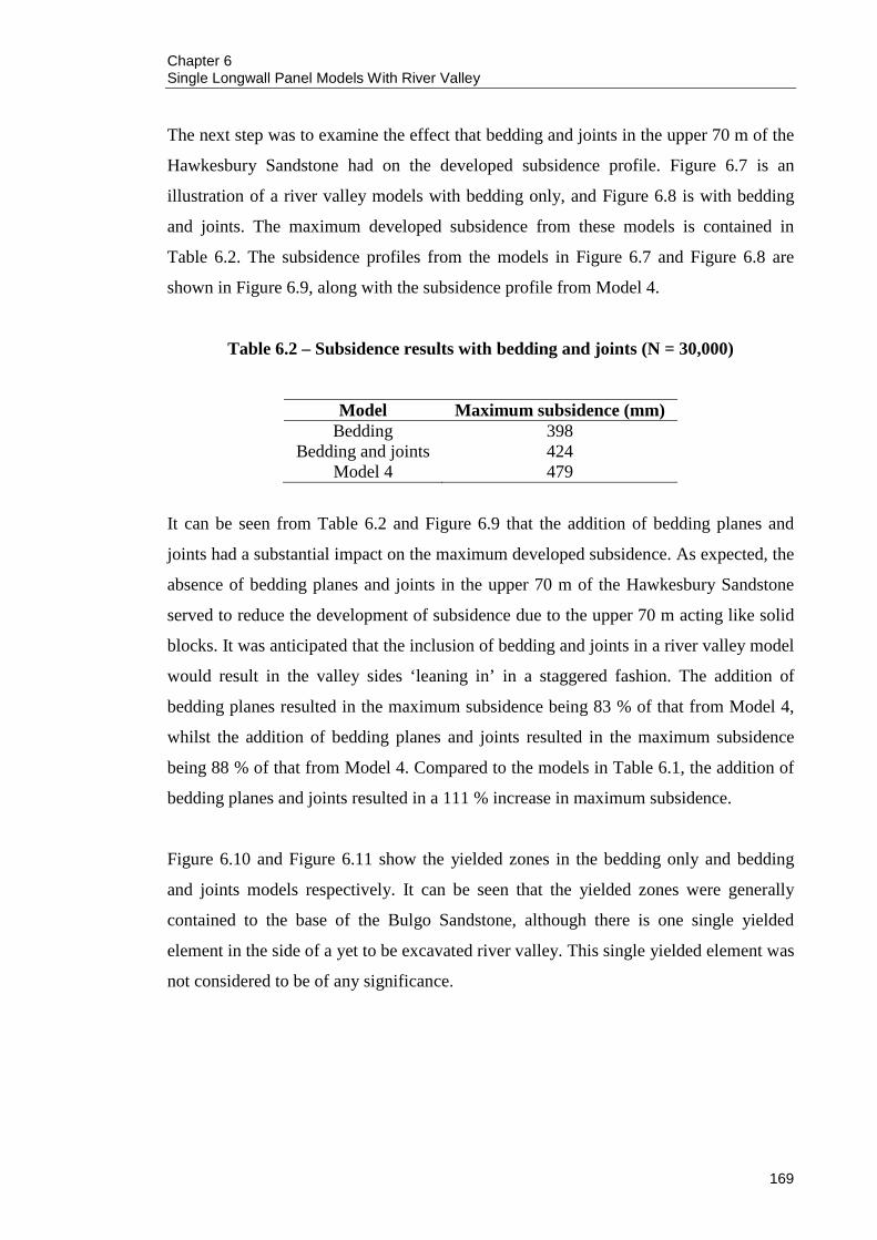
Chapter 6 Single Longwall Panel Models With River Valley
169
The next step was to examine the effect that bedding and joints in the upper 70 m of the
Hawkesbury Sandstone had on the developed subsidence profile. Figure 6.7 is an
illustration of a river valley models with bedding only, and Figure 6.8 is with bedding
and joints. The maximum developed subsidence from these models is contained in
Table 6.2. The subsidence profiles from the models in Figure 6.7 and Figure 6.8 are
shown in Figure 6.9, along with the subsidence profile from Model 4.
Table 6.2 – Subsidence results with bedding and joints (N = 30,000)
Model Maximum subsidence (mm) Bedding 398
Bedding and joints 424 Model 4 479
It can be seen from Table 6.2 and Figure 6.9 that the addition of bedding planes and
joints had a substantial impact on the maximum developed subsidence. As expected, the
absence of bedding planes and joints in the upper 70 m of the Hawkesbury Sandstone
served to reduce the development of subsidence due to the upper 70 m acting like solid
blocks. It was anticipated that the inclusion of bedding and joints in a river valley model
would result in the valley sides ‘leaning in’ in a staggered fashion. The addition of
bedding planes resulted in the maximum subsidence being 83 % of that from Model 4,
whilst the addition of bedding planes and joints resulted in the maximum subsidence
being 88 % of that from Model 4. Compared to the models in Table 6.1, the addition of
bedding planes and joints resulted in a 111 % increase in maximum subsidence.
Figure 6.10 and Figure 6.11 show the yielded zones in the bedding only and bedding
and joints models respectively. It can be seen that the yielded zones were generally
contained to the base of the Bulgo Sandstone, although there is one single yielded
element in the side of a yet to be excavated river valley. This single yielded element was
not considered to be of any significance.

Chapter 6 Single Longwall Panel Models With River Valley
170
Fig. 6.7 – Model with bedding in upper 70 m of Hawkesbury Sandstone

Chapter 6 Single Longwall Panel Models With River Valley
171
Fig. 6.8 – Model with bedding and joints in upper 70 m of Hawkesbury Sandstone
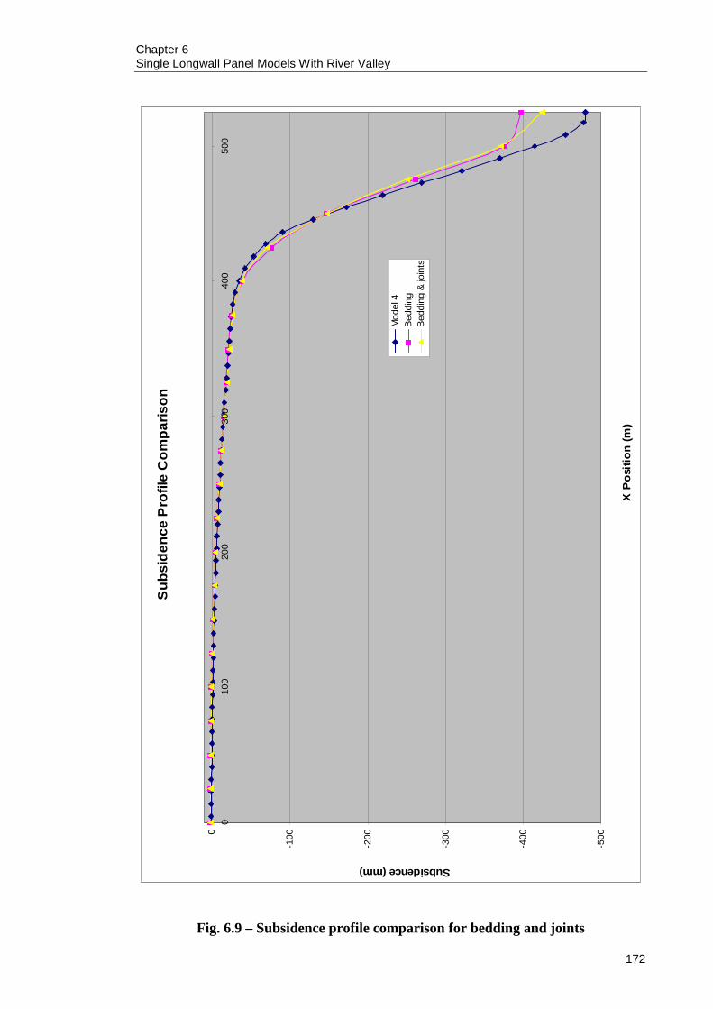
Chapter 6 Single Longwall Panel Models With River Valley
172
Fig. 6.9 – Subsidence profile comparison for bedding and joints
Sub
side
nce
Pro
file
Com
paris
on
-500
-400
-300
-200
-1000
010
020
030
040
050
0
X P
ositi
on (m
)
Subsidence (mm)
Mod
el 4
Bed
ding
Bed
ding
& jo
ints

Chapter 6 Single Longwall Panel Models With River Valley
173
Fig. 6.10 – Yielded zones in a river valley model with bedding
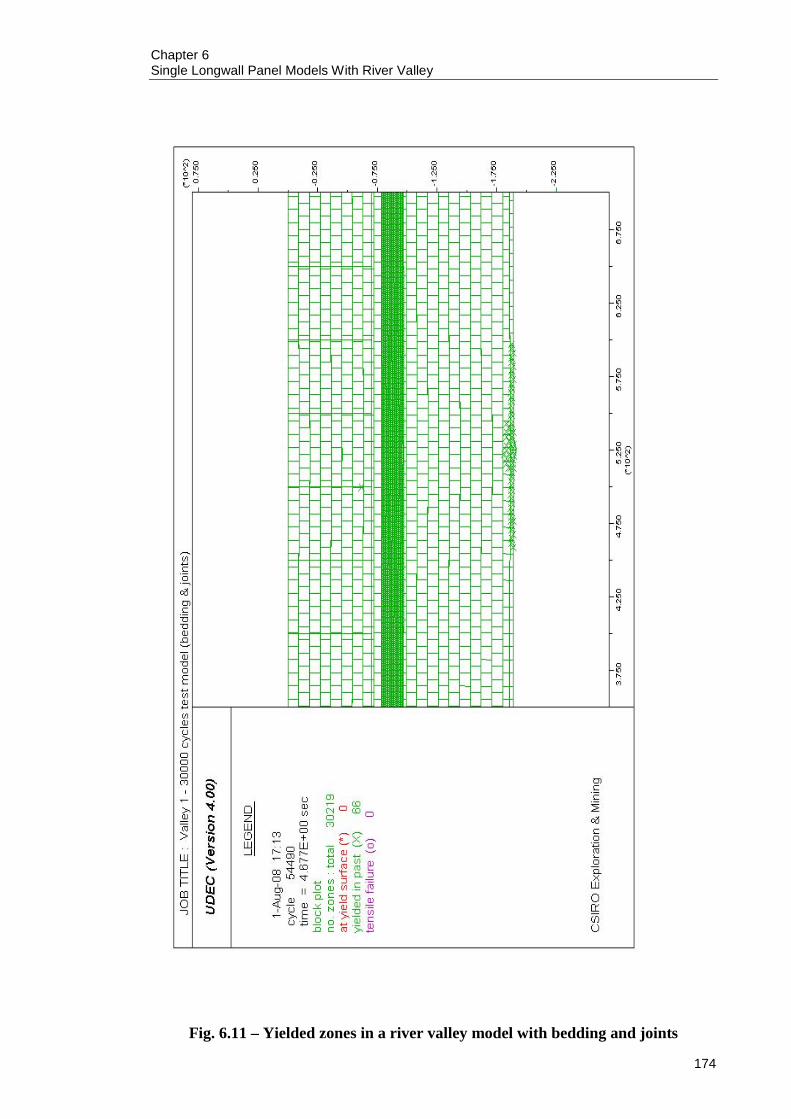
Chapter 6 Single Longwall Panel Models With River Valley
174
Fig. 6.11 – Yielded zones in a river valley model with bedding and joints
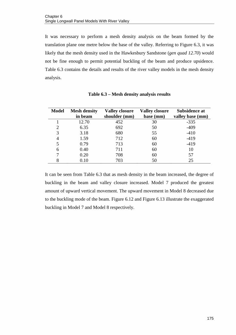
Chapter 6 Single Longwall Panel Models With River Valley
175
It was necessary to perform a mesh density analysis on the beam formed by the
translation plane one metre below the base of the valley. Referring to Figure 6.3, it was
likely that the mesh density used in the Hawkesbury Sandstone (gen quad 12.70) would
not be fine enough to permit potential buckling of the beam and produce upsidence.
Table 6.3 contains the details and results of the river valley models in the mesh density
analysis.
Table 6.3 – Mesh density analysis results
Model Mesh density in beam
Valley closure shoulder (mm)
Valley closure base (mm)
Subsidence at valley base (mm)
1 12.70 452 30 -335 2 6.35 692 50 -409 3 3.18 680 55 -410 4 1.59 712 60 -419 5 0.79 713 60 -419 6 0.40 711 60 10 7 0.20 708 60 57 8 0.10 703 50 25
It can be seen from Table 6.3 that as mesh density in the beam increased, the degree of
buckling in the beam and valley closure increased. Model 7 produced the greatest
amount of upward vertical movement. The upward movement in Model 8 decreased due
to the buckling mode of the beam. Figure 6.12 and Figure 6.13 illustrate the exaggerated
buckling in Model 7 and Model 8 respectively.

Chapter 6 Single Longwall Panel Models With River Valley
176
Fig. 6.12 – Beam buckling in Model 7
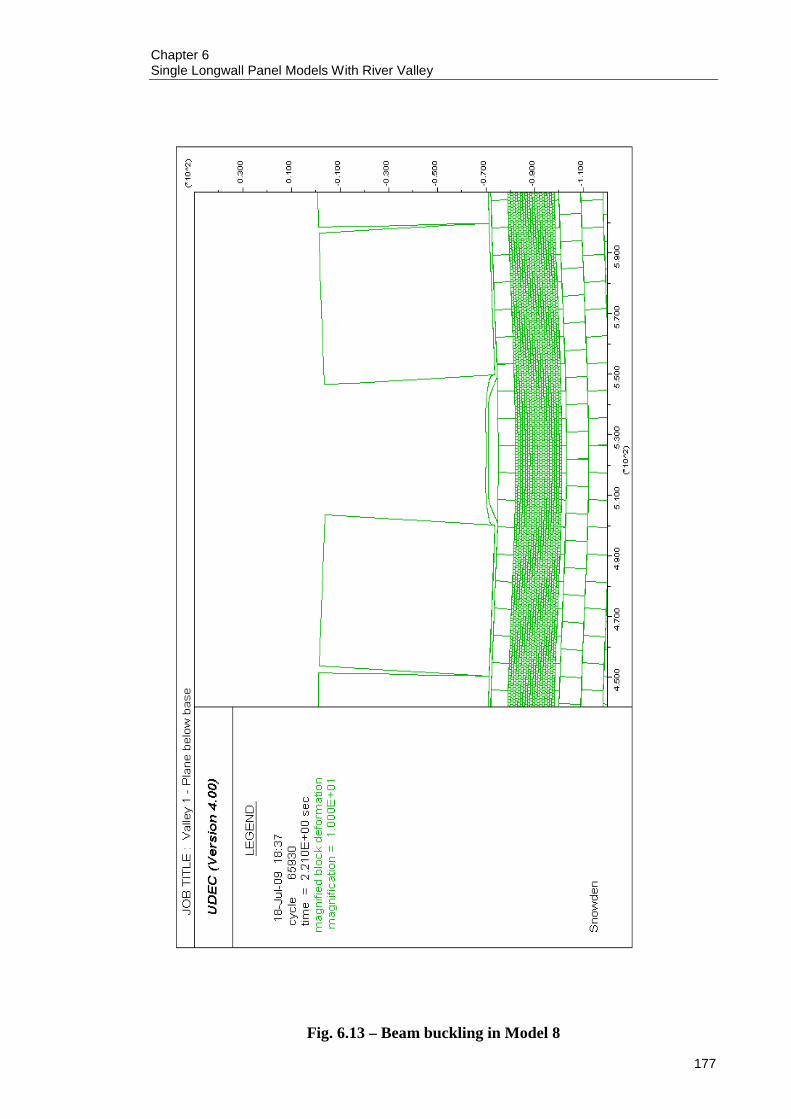
Chapter 6 Single Longwall Panel Models With River Valley
177
Fig. 6.13 – Beam buckling in Model 8

Chapter 6 Single Longwall Panel Models With River Valley
178
It was decided to use the mesh density in Model 7, as it produced the greatest amount of
vertical upward movement in the valley and represented simple buckling.
It was concluded that the initial models successfully identified the appropriate number
of cycles (N = 30,000) to be applied to the model by analysis of maximum developed
subsidence and run times. The initial models also sufficiently demonstrated that the base
of the models was at an acceptable distance from the base of the proposed river valleys,
and the methodology of deforming the base of the models exactly replicated the Bulgo
Sandstone profile in Model 4. The subsidence profiles from the initial models were
considered sufficient enough to conduct an analysis with the river valley models. As
stated previously, the sole purpose of the modelling was to investigate the block
movement theory, and an attempt has been made to produce reasonable deformations in
order to enable this.
6.4 RIVER VALLEY MODELS
Following on from the initial models and mesh density analysis, a total of fifty river
valley models were created based on the following variations and characteristics:
No bedding and joints in upper 70 m of Hawkesbury Sandstone
o Translation plane at base
o Translation plane below base
No joints in beam formed by translation plane
Joints in beam formed by translation plane
Bedding and joints in upper 70 m of Hawkesbury Sandstone
o Translation plane at base
o Translation plane below base
There were five major parameters that were changed throughout the analysis. These
were the position of the valley relative to the longwall centreline, the location of the
translation plane, bedding and joints in the upper 70 m of the Hawkesbury Sandstone,
and the addition of vertical joints in the beam formed when the translation plane was
one metre below the base of the valleys.

Chapter 6 Single Longwall Panel Models With River Valley
179
Varying the position of the valley relative to the longwall panel allowed assessment of
horizontal and vertical movements in the area above unmined coal (hogging phase).
Moving the location of the translation plane from the base of the valleys to one metre
below the valley base permitted examination of the proposed theory that valley closure
is reduced when the translation plane is below the base of the valley. Adding bedding
and joints in the upper 70 m of the Hawkesbury Sandstone was done to test the model
against the rigid body observation by Holla and Barclay (2000). Adding joints to the
beam formed by the translation plane beneath the base of the valley was done to
ascertain if this had any effect on subsidence and valley closure.
The definition of upsidence given by Waddington Kay and Associates (2002) is “a
reduction in the expected quantum of subsidence at a point, being the difference
between the predicted or estimated subsidence and the vertical displacement actually
measured”. Using this definition, it is possible to measure upsidence in an existing
valley by comparing the difference in subsidence at the base of a valley when variations
are performed on the model. It must be noted that the above definition is not conclusive.
Upsidence could also be defined as direct upward movement in a river valley base as a
result of base yield and buckling. In the models, it was decided to use the Waddington
Kay and Associates definition to distinguish if it yielded conclusive results.
Figure 6.14 is a representative view of a typical valley model with no bedding or joints
in the upper 70 m of the Hawkesbury Sandstone. In this figure, the valley centreline
corresponds with the longwall centreline. In the river valley models, the location of the
valley varied in the left hand side of the model.
Figure 6.15 is a close up view of a valley with no bedding or joints in the upper 70 m of
the Hawkesbury Sandstone, with the translation plane at the base of the valley.
Figure 6.16 is a close up view of a valley with no bedding or joints in the upper 70 m of
the Hawkesbury Sandstone, with the translation plane one metre below the base of the
valley. Figure 6.17 is a close up view of a valley with bedding planes and joints in the
upper 70 m of the Hawkesbury Sandstone, with the translation plane at the base of the
valley. Figure 6.18 is a close up view of a valley with bedding planes and joints in the
upper 70 m of the Hawkesbury Sandstone, with the translation plane one metre below
the base of the valley. Figure 6.19 is a close up view of a valley with no bedding and

Chapter 6 Single Longwall Panel Models With River Valley
180
joints in the upper 70 m of the Hawkesbury Sandstone, with the translation plane one
metre below the base of the valley and with joints in the beam formed by the translation
plane.
The modelling procedure for the river valley models was as follows:
1. Create geometry, assign properties, boundary conditions, in-situ stress regime
and cycle to equilibrium,
2. Excavate required valley and cycle to equilibrium,
3. Reset velocities, displacements and boundary conditions,
4. Apply roller boundaries to the sides of the model,
5. Cycle for one step to obtain the time step,
6. Identify grid points at the base of the model to which velocities will be attached,
7. Define the maximum displacement for each previously identified grid point (as
derived from the displacement profile for the Bulgo Sandstone in Model 4),
8. Calculate the y velocity for the identified grid points using V = D/∆tN,
9. Assign y velocities to grid points,
10. Cycle model for N (30,000) cycles to obtain required displacement at base,
11. Reset boundary conditions and place roller boundaries on each side of model,
and
12. Cycle model for an additional 20,000 cycles to ensure final equilibrium is
reached.

Chapter 6 Single Longwall Panel Models With River Valley
181
Fig. 6.14 – Typical river valley model

Chapter 6 Single Longwall Panel Models With River Valley
182
Fig. 6.15 – Translation plane at base of valley

Chapter 6 Single Longwall Panel Models With River Valley
183
Fig. 6.16 – Translation plane below base of valley
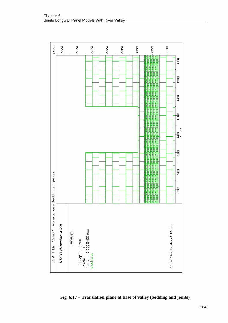
Chapter 6 Single Longwall Panel Models With River Valley
184
Fig. 6.17 – Translation plane at base of valley (bedding and joints)

Chapter 6 Single Longwall Panel Models With River Valley
185
Fig. 6.18 – Translation plane below base of valley (bedding and joints)

Chapter 6 Single Longwall Panel Models With River Valley
186
Fig. 6.19 – Translation plane below base of valley (joints in beam)

Chapter 6 Single Longwall Panel Models With River Valley
187
X-displacement history points were placed on the shoulders of each valley, along with
y-displacement history points that were placed on the centre of the valley floor. These
history points were monitored for each individual valley in question and the models
were investigated to see whether they conformed to the expected behaviour i.e.
increased valley closure and minimal valley base yield with a translation plane at the
base of a valley, and decreased valley closure with increased valley base yield with the
translation plane one metre below the valley floor.
6.5 RESULTS
The results from the valley models are shown in Tables 6.4 to 6.8. Figure 6.20 and
Figure 6.21 are the subsidence profiles prior to valley excavation for the models (no
bedding and joints in the upper 70 m of the Hawkesbury Sandstone, and bedding and
joints in the upper 70 m of the Hawkesbury Sandstone). Figure 6.22 and Figure 6.23 are
the corresponding tilt profiles. Figure 6.24 and Figure 6.29 illustrate the subsidence at
the base of the valley as a function of distance from the longwall centreline. Figure 6.33
and Figure 6.34 illustrate the valley closure at the shoulders of the valleys as a function
of distance from the longwall centreline. Figure 6.41 and Figure 6.42 illustrate the
valley closure at the base of the valleys as a function of distance from the longwall
centreline.
Table 6.4 – No bedding and joints in the upper 70 m of Hawkesbury Sandstone,
translation plane at base
Valley Valley centre to longwall centre
(m)
Valley closure shoulder
(mm)
Valley closure base
(mm)
Subsidence at valley base
(mm) 1 0 727 70 -423 2 50 413 195 -266 3 100 138 432 -71 4 150 72 175 -26 5 200 64 89 -18 6 250 46 58 -10 7 300 35 39 -5 8 350 22 28 -2 9 400 7 11 0
10 450 -3 0 2

Chapter 6 Single Longwall Panel Models With River Valley
188
Table 6.5 – No bedding and joints in the upper 70 m of Hawkesbury Sandstone,
translation plane below base, no joints in beam
Valley Valley centre to longwall centre
(m)
Valley closure shoulder
(mm)
Valley closure base
(mm)
Subsidence at valley base
(mm) 1 0 708 45 57 2 50 323 35 14 3 100 166 56 -12 4 150 25 66 -27 5 200 24 46 -17 6 250 27 33 -10 7 300 18 22 -5 8 350 8 10 -1 9 400 4 0 0
10 450 -2 0 2
Table 6.6 – No bedding and joints in the upper 70 m of Hawkesbury Sandstone,
translation plane below base, joints in beam
Valley Valley centre to longwall centre
(m)
Valley closure shoulder
(mm)
Valley closure base
(mm)
Subsidence at valley base
(mm) 1 0 701 60 50 2 50 331 45 12 3 100 171 60 -12 4 150 29 76 -27 5 200 30 54 -17 6 250 28 38 -9 7 300 20 22 -5 8 350 6 9 -2 9 400 0 3 1
10 450 -3 0 2

Chapter 6 Single Longwall Panel Models With River Valley
189
Table 6.7 – Bedding and joints in the upper 70 m of Hawkesbury Sandstone,
translation plane at base
Valley Valley centre to longwall centre
(m)
Valley closure shoulder
(mm)
Valley closure base
(mm)
Subsidence at valley base
(mm) 1 0 693 55 -415 2 50 349 128 -289 3 100 146 158 -57 4 150 111 96 -27 5 200 89 94 -18 6 250 72 77 -10 7 300 54 55 -5 8 350 31 32 -2 9 400 14 16 1
10 450 1 4 2
Table 6.8 – Bedding and joints in the upper 70 m of Hawkesbury Sandstone,
translation plane below base
Valley Valley centre to longwall centre
(m)
Valley closure shoulder
(mm)
Valley closure base
(mm)
Subsidence at valley base
(mm) 1 0 685 55 46 2 50 348 50 24 3 100 134 26 -21 4 150 104 33 -27 5 200 86 28 -18 6 250 67 15 -11 7 300 47 5 -6 8 350 32 4 -1 9 400 14 4 0
10 450 1 3 2
6.5.1 Subsidence without valley excavation
From Figure 6.20, it can be seen that when the translation plane was at the base of the
valley and no bedding and joints were present in the upper 70m of Hawkesbury
Sandstone, the maximum developed subsidence was 201 mm. This was to be expected
as this model was the same as the model in Table 6.1 (N = 30,000).
Chapter 6 Single Longwall Panel Models With River Valley
190
When the translation plane was moved one metre below the base of the valley, it can be
seen from Figure 6.20 that the maximum developed subsidence reduced to 198 mm.
When joints were added to the beam formed by the translation plane, it can be seen
from Figure 6.18 that the maximum developed subsidence increased to 199 mm.
When bedding and joints were added to the upper 70 m of Hawkesbury Sandstone and
the translation plane was at the base of the valleys, it can be seen from Figure 6.21 that
the maximum developed subsidence was 411 mm. When the translation plane was
moved one metre below the valley base, it can be seen from Figure 6.21 that the
maximum developed subsidence was 419 mm. The increase in maximum developed
subsidence when bedding and joints were added to the upper 70 m of the Hawkesbury
Sandstone was expected, due to the increased flexibility of the model afforded by the
extra discontinuities.
The models prior to valley excavation show that the model results were consistent and
did not vary substantially prior to valley excavation. This establishes a stable numerical
modelling base when valleys are excavated. For example, when bedding and joints were
not present in the upper 70 m of Hawkesbury Sandstone, the maximum variation in
subsidence was in the order of 3 mm. When bedding and joints were present, the
maximum variation was 8 mm.

Chapter 6 Single Longwall Panel Models With River Valley
191
Fig. 6.20 – Subsidence prior to valley excavation (no bedding and joints in upper
70 m of Hawkesbury Sandstone)
Sub
side
nce
Pro
file
-220
-200
-180
-160
-140
-120
-100-80
-60
-40
-200
020
040
060
080
010
00
X P
ositi
on (m
)
Subsidence (mm)
Tran
slat
ion
plan
e at
bas
eTr
ansl
atio
n pl
ane
belo
w b
ase,
no
join
ts in
bea
mTr
ansl
atio
n pl
ane
belo
w b
ase,
join
ts in
bea
m
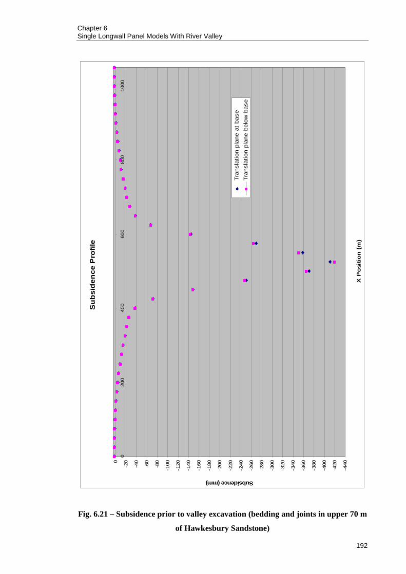
Chapter 6 Single Longwall Panel Models With River Valley
192
Fig. 6.21 – Subsidence prior to valley excavation (bedding and joints in upper 70 m
of Hawkesbury Sandstone)
Su
bsi
den
ce P
rofil
e
-440
-420
-400
-380
-360
-340
-320
-300
-280
-260
-240
-220
-200
-180
-160
-140
-120
-100-80
-60
-40
-200
020
040
060
080
010
00
X P
osi
tion
(m)
Subsidence (mm)
Tran
slat
ion
plan
e at
bas
eTr
ansl
atio
n pl
ane
belo
w b
ase

Chapter 6 Single Longwall Panel Models With River Valley
193
6.5.2 Tilt without valley excavation
It can be seen in Figure 6.22 when the translation plane was at the base of the valley; the
average maximum tilt was 3.89 mm/m. The point of maximum tilt (or inflection point)
was located 62.50 m from the longwall centreline. When the translation plane was
moved one metre below the base of the valley (Figure 6.22), the average maximum tilt
reduced to 3.83 mm/m, and the point of maximum tilt was also located 62.50 m from
the longwall centreline. When joints were added to the beam formed by the translation
plane, it can be seen from Figure 6.22 that the average tilt increased to 3.87 mm/m. The
position of maximum tilt was also located 62.50 m from the longwall centreline.
When bedding and joints were added to the upper 70 m of the Hawkesbury Sandstone,
it can be seen from Figure 6.23 that when the translation plane was at the base of the
valley, the average maximum tilt was 4.90 mm/m. The point of maximum tilt was
located 37.50 m from the longwall centreline. When the translation plane was moved
one metre below the base of the valley (Figure 6.23), the average maximum tilt
decreased to 4.77 mm/m, and the point of maximum tilt was also located 37.50 m from
the longwall centreline.
The tilt results prior to valley excavation illustrate a stable numerical modelling
platform, like the subsidence results prior to valley excavation. The difference in the
magnitude of tilt and the location of the position of maximum tilt when bedding and
joints were added to the upper 70 m of the Hawkesbury Sandstone can be attributed to
the increased flexibility of the model, and the resulting increased subsidence and altered
shape of the subsidence profile.
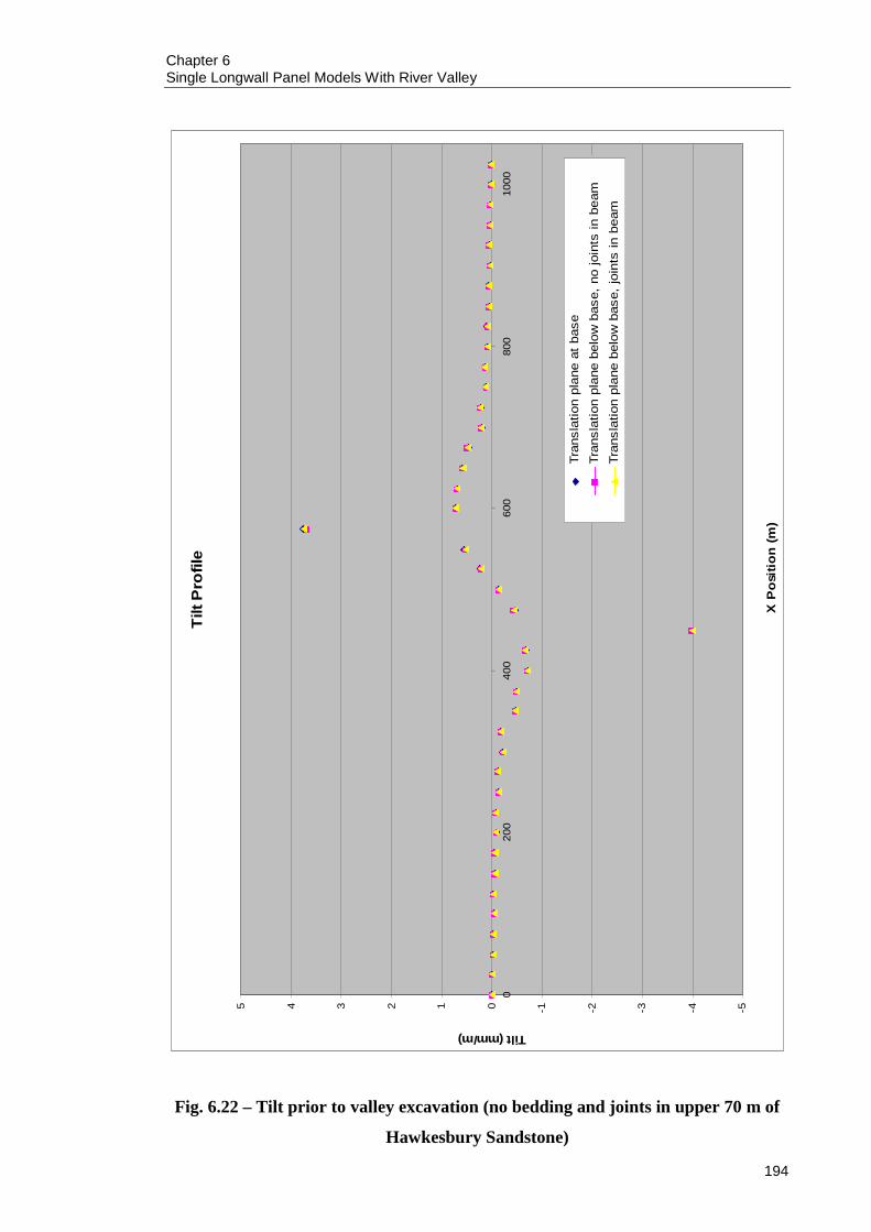
Chapter 6 Single Longwall Panel Models With River Valley
194
Fig. 6.22 – Tilt prior to valley excavation (no bedding and joints in upper 70 m of
Hawkesbury Sandstone)
Tilt
Pro
file
-5-4-3-2-1012345
020
040
060
080
010
00
X P
ositi
on (m
)
Tilt (mm/m)
Tran
slat
ion
plan
e at
bas
eTr
ansl
atio
n pl
ane
belo
w b
ase,
no
join
ts in
bea
mTr
ansl
atio
n pl
ane
belo
w b
ase,
join
ts in
bea
m

Chapter 6 Single Longwall Panel Models With River Valley
195
Fig. 6.23 – Tilt prior to valley excavation (bedding and joints in upper 70 m of
Hawkesbury Sandstone)
Tilt
Pro
file
-6-5-4-3-2-10123456
020
040
060
080
010
00
X P
ositi
on
(m)
Tilt (mm/m)
Tran
slat
ion
plan
e at
bas
eTr
ansl
atio
n pl
ane
belo
w b
ase

Chapter 6 Single Longwall Panel Models With River Valley
196
6.5.3 Subsidence/upsidence at base of valleys
The subsidence results and the calculated upsidence are shown in Tables 6.9 to 6.11.
Table 6.9 – Upsidence between models in Table 6.4 and Table 6.5
Valley Valley centre to longwall centre (m)
Subsidence (mm, Table 6.4)
Subsidence (mm, Table 6.5)
Upsidence (mm)
1 0 -423 57 480 2 50 -266 14 280 3 100 -71 -12 59 4 150 -26 -27 -1 5 200 -18 -17 1 6 250 -10 -10 0 7 300 -5 -5 0 8 350 -2 -1 1 9 400 0 0 0
10 450 2 2 0
Table 6.10 – Upsidence between models in Table 6.4 and Table 6.6
Valley Valley centre to longwall centre (m)
Subsidence (mm, Table 6.4)
Subsidence (mm, Table 6.6)
Upsidence (mm)
1 0 -423 50 473 2 50 -266 12 278 3 100 -71 -12 59 4 150 -26 -27 -1 5 200 -18 -17 1 6 250 -10 -9 1 7 300 -5 -5 0 8 350 -2 -2 0 9 400 0 1 1
10 450 2 2 0

Chapter 6 Single Longwall Panel Models With River Valley
197
Table 6.11 – Upsidence between models in Table 6.7 and Table 6.8
Valley Valley centre to longwall centre (m)
Subsidence (mm, Table 6.7)
Subsidence (mm, Table 6.8)
Upsidence (mm)
1 0 -415 46 461 2 50 -289 24 313 3 100 -57 -21 36 4 150 -27 -27 0 5 200 -18 -18 0 6 250 -10 -11 -1 7 300 -5 -6 -1 8 350 -2 -1 1 9 400 1 0 -1
10 450 2 2 0
When the upper 70 m of Hawkesbury Sandstone contained no bedding and joints, it can
be seen from Table 6.9, Table 6.10 and Figure 6.24 that upsidence was produced when
the translation plane was located below the base of the valley, but not when the location
plane was located at the base of the valley.
From Table 6.9, it can be seen that moving the translation plane one metre below the
base of the valleys and not adding any joints to the beam formed by the translation
plane produced a maximum upsidence of 480 mm above the longwall centreline,
280 mm at 50 m from the longwall centreline, and 59 mm at 100 m from the longwall
centreline.
Figures 6.25 to 6.27 are plots of the exaggerated block deformations when the centreline
of the valley was at 0 m, 50 m and 100 m from the longwall centreline respectively,
with the plane below the valley base and no bedding and joints in the upper 70 m of
Hawkesbury Sandstone.
Given that the river valley models are based on Model 4 in Chapter 5, which has a
longwall width of 175 m, it can be seen that upsidence occurred outside the goaf edge,
and not solely above the longwall centreline.
From Table 6.10 and Figure 6.24, it can be seen that the addition of vertical joints in the
beam formed by the translation plane produced very little difference in terms of
subsidence and calculated upsidence. Figure 6.28 is a block deformation plot of a valley

Chapter 6 Single Longwall Panel Models With River Valley
198
above the longwall centreline, with joints in the beam formed by the translation plane.
Shear displacements are also illustrated and it can be seen that no shear occurred in the
vertical joints.
When bedding and joints were added to the upper 70 m of Hawkesbury Sandstone, it
can be seen from Table 6.11 and Figure 6.29 that the subsidence and calculated
upsidence was generally less outside the goaf edge. Figure 6.30 is a plot of block
deformations and shear displacements outside the goaf edge (100 m from the longwall
centreline), and it can be seen that as the rock mass was being forced into the free face
provided by the valley, the increased shear displacements in the walls of the valley
alleviated the horizontal stress concentration in the corner of the valley closest to the
longwall centreline, which is illustrated in Figure 6.31 and Figure 6.32. It can be seen
from Figure 6.31 and Figure 6.32 that when the model contained no bedding and joints
in the upper 70 m of Hawkesbury Sandstone, a horizontal compressive stress of 85 MPa
was concentrated in the corner of the valley, and when the model contained bedding and
joints in the upper 70 m of Hawkesbury Sandstone, the concentration of compressive
stress in the corner of the valley reduced to 27.5 MPa.
It can also be seen from Table 6.11 and Figure 6.29 that the amount of subsidence
influenced upsidence. When bedding and joints were added to the upper 70 m of
Hawkesbury Sandstone, it can be seen that the upsidence at 50 m from the longwall
centreline (313 mm) was greater than the models with no bedding and joints in the
upper 70 m of Hawkesbury Sandstone. Likewise, a greater amount of subsidence had
occurred in this location. It was previously demonstrated in Figure 6.31 and Figure 6.32
that the addition of bedding and joints in the upper 70 m of Hawkesbury Sandstone
served to reduce the concentration of compressive stress in the valley. This occurrence
of upsidence which was greater than the upsidence produced by rigid block movements
at the same location illustrates that horizontal compressive stress redistribution is not
the primary mechanism behind upsidence, rather the subsidence profile with its
associated tilts and curvatures are.
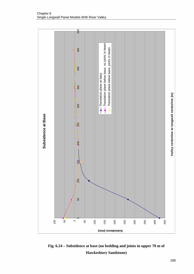
Chapter 6 Single Longwall Panel Models With River Valley
199
Fig. 6.24 – Subsidence at base (no bedding and joints in upper 70 m of
Hawkesbury Sandstone)
Sub
side
nce
at B
ase
-450
-400
-350
-300
-250
-200
-150
-100-50050100
050
100
150
200
250
300
350
400
450
500
Val
ley
cent
relin
e to
long
wal
l cen
trel
ine
(m)
Subsidence (mm)
Tran
slat
ion
plan
e at
bas
eTr
ansl
atio
n pl
ane
belo
w b
ase,
no
join
ts in
bea
mTr
ansl
atio
n pl
ane
belo
w b
ase,
join
ts in
bea
m

Chapter 6 Single Longwall Panel Models With River Valley
200
Fig. 6.25 – Exaggerated block deformations when valley is 0 m from longwall
centreline (no bedding and joints in upper 70 m of Hawkesbury Sandstone)
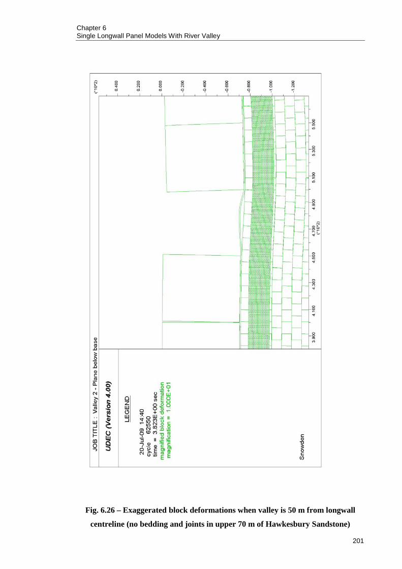
Chapter 6 Single Longwall Panel Models With River Valley
201
Fig. 6.26 – Exaggerated block deformations when valley is 50 m from longwall
centreline (no bedding and joints in upper 70 m of Hawkesbury Sandstone)

Chapter 6 Single Longwall Panel Models With River Valley
202
Fig. 6.27 – Exaggerated block deformations when valley is 100 m from longwall
centreline (no bedding and joints in upper 70 m of Hawkesbury Sandstone)

Chapter 6 Single Longwall Panel Models With River Valley
203
Fig. 6.28 – Block deformations and shear when valley is 0 m from longwall
centreline (no bedding and joints in upper 70 m of Hawkesbury Sandstone, joints
in beam)
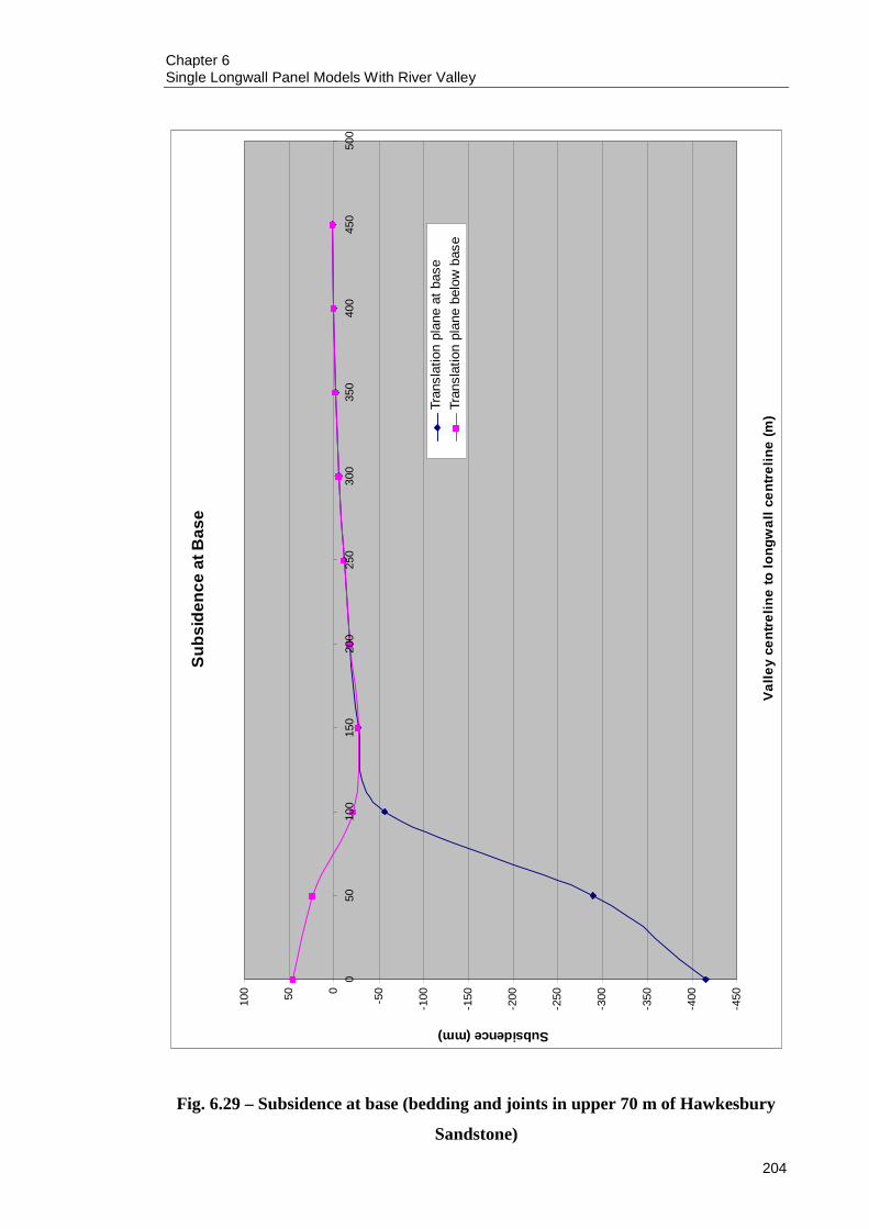
Chapter 6 Single Longwall Panel Models With River Valley
204
Fig. 6.29 – Subsidence at base (bedding and joints in upper 70 m of Hawkesbury
Sandstone)
Sub
side
nce
at B
ase
-450
-400
-350
-300
-250
-200
-150
-100-50050100
050
100
150
200
250
300
350
400
450
500
Val
ley
cent
relin
e to
long
wal
l cen
trel
ine
(m)
Subsidence (mm)
Tran
slat
ion
plan
e at
bas
eTr
ansl
atio
n pl
ane
belo
w b
ase

Chapter 6 Single Longwall Panel Models With River Valley
205
Fig. 6.30 – Block deformation and shear when valley is 100 m from longwall
centreline (bedding and joints in upper 70 m of Hawkesbury Sandstone)

Chapter 6 Single Longwall Panel Models With River Valley
206
Fig. 6.31 – Horizontal stress when valley is 100 m from longwall centreline (no
bedding and joints in upper 70 m of Hawkesbury Sandstone)

Chapter 6 Single Longwall Panel Models With River Valley
207
Fig. 6.32 – Horizontal stress when valley is 100 m from longwall centreline
(bedding and joints in upper 70 m of Hawkesbury Sandstone)

Chapter 6 Single Longwall Panel Models With River Valley
208
6.5.4 Valley closure at shoulders
It can be seen from Figure 6.33 and Figure 6.34 that the general trend in closure was for
the maximum to be above the centre of the longwall panel, and reducing as the distance
from the longwall centreline increased. When valleys are represented as blocks sliding
on a plane, the closure at the valley shoulders is a function of the geometry of the
subsidence profile, hence the greatest closure above the longwall centreline. This is
illustrated in Figure 6.35.
When the upper 70 m of the Hawkesbury Sandstone contained no bedding or joints, it
can be seen from Figure 6.33 that the most valley closure was produced when the
translation plane was at the base of the valley. When the translation plane was moved
underneath the base of the valley by one metre, and there were no joints in the beam
formed by the translation plane, valley closure at the shoulders was reduced by an
average of 37 %. The greatest reduction as a percentage of original closure occurred at
the point 150 m away from the longwall centreline, where a 65 % reduction in closure
occurred.
In Figure 6.33, the closure occurring when the translation plane was beneath the base of
the valley exceeded the closure when the translation plane was at the base of the valley
when the valley was 100 m from the longwall centreline. An examination of the block
movements in both of these cases revealed that when the beam was beneath the base of
the valley, it was buckling not only at the valley base, but also adjacent to the valley.
This resulted in the block adjacent to the valley being tilted towards the valley which
produced the greater valley closure. This is illustrated in Figure 6.36 and Figure 6.37.

Chapter 6 Single Longwall Panel Models With River Valley
209
Fig. 6.33 – Valley closure at shoulders (no bedding and joints in upper 70 m of
Hawkesbury Sandstone)
Val
ley
Clo
sure
at S
houl
ders
-1000
100
200
300
400
500
600
700
800
050
100
150
200
250
300
350
400
450
500
Val
ley
cent
relin
e to
long
wal
l cen
trel
ine
(m)
Closure (mm)
Tran
slat
ion
plan
e at
bas
eTr
ansl
atio
n pl
ane
belo
w b
ase,
no
join
ts in
bea
mTr
ansl
atio
n pl
ane
belo
w b
ase,
join
ts in
bea
m

Chapter 6 Single Longwall Panel Models With River Valley
210
Fig. 6.34 – Valley closure at shoulders (bedding and joints in upper 70 m of
Hawkesbury Sandstone)
Val
ley
Clo
sure
at S
houl
ders
0
100
200
300
400
500
600
700
800
050
100
150
200
250
300
350
400
450
500
Val
ley
cent
relin
e to
long
wal
l cen
trel
ine
(m)
Closure (mm)
Tran
slat
ion
plan
e at
bas
eTr
ansl
atio
n pl
ane
belo
w b
ase

Chapter 6 Single Longwall Panel Models With River Valley
211
Fig. 6.35 – Exaggerated displacements above longwall centreline, plane at base

Chapter 6 Single Longwall Panel Models With River Valley
212
Fig. 6.36 – Exaggerated displacements, plane at base

Chapter 6 Single Longwall Panel Models With River Valley
213
Fig. 6.37 – Exaggerated displacements, plane below base

Chapter 6 Single Longwall Panel Models With River Valley
214
When joints were added to the beam formed by the translation plane, it can be seen
from Figure 6.33 that the magnitude of closure was generally the same compared to the
models with no joints in the beam. This was to be expected, as the presence of joints in
the beam formed by the translation plane did not increase the maximum developed
subsidence substantially, compared to when the joints were absent.
It can be seen from Tables 6.4 to 6.6 that closure at the shoulders was negative around
450 m from the longwall centreline. This was a result of the modelling procedure,
where the sides of the models were fixed, so the last valley actually opened up as the
subsidence profile formed (Figure 6.38). In some instances valley closure was still
positive, but the magnitude of closure involved is in the order of millimetres and as
such, was ignored in this analysis.
When the upper 70 m of the Hawkesbury Sandstone contained bedding and joints, it can
be seen from Figure 6.34 there was very little difference in closure at the valley
shoulders between the translation plane at the base of the valleys, and the translation
plane below the base of the valleys. Accordingly, there were no instances of yield in the
valley bases in the models where the translation plane was at the base of the valleys, due
to slip along bedding in the upper 70 m of Hawkesbury Sandstone resulting in the valley
walls being pushed into the valley in a staggered pattern and releasing any build up of
horizontal stresses (Figure 6.30). As such, this lends support to the observation by Holla
and Barclay (2000) that rigid block type movements occur out in the field.
Figure 6.39 is an illustration of the tensile areas around a valley that was 350 m from
the longwall centreline. Figure 6.40 is an illustration of valley closure in the same valley
when the translation plane was at the base of the valley – this figure confirms that valley
closure in the tensile portion of the subsidence profile is a result of blocks being pushed
into the void created by the valley.

Chapter 6 Single Longwall Panel Models With River Valley
215
Fig. 6.38 – Example of negative valley closure due to boundary conditions

Chapter 6 Single Longwall Panel Models With River Valley
216
Fig. 6.39 – Tensile areas around valley located 350 m from longwall centreline,
plane at base

Chapter 6 Single Longwall Panel Models With River Valley
217
Fig. 6.40 – Valley closure when translation plane is at the base of the valley, 350 m
from longwall centreline
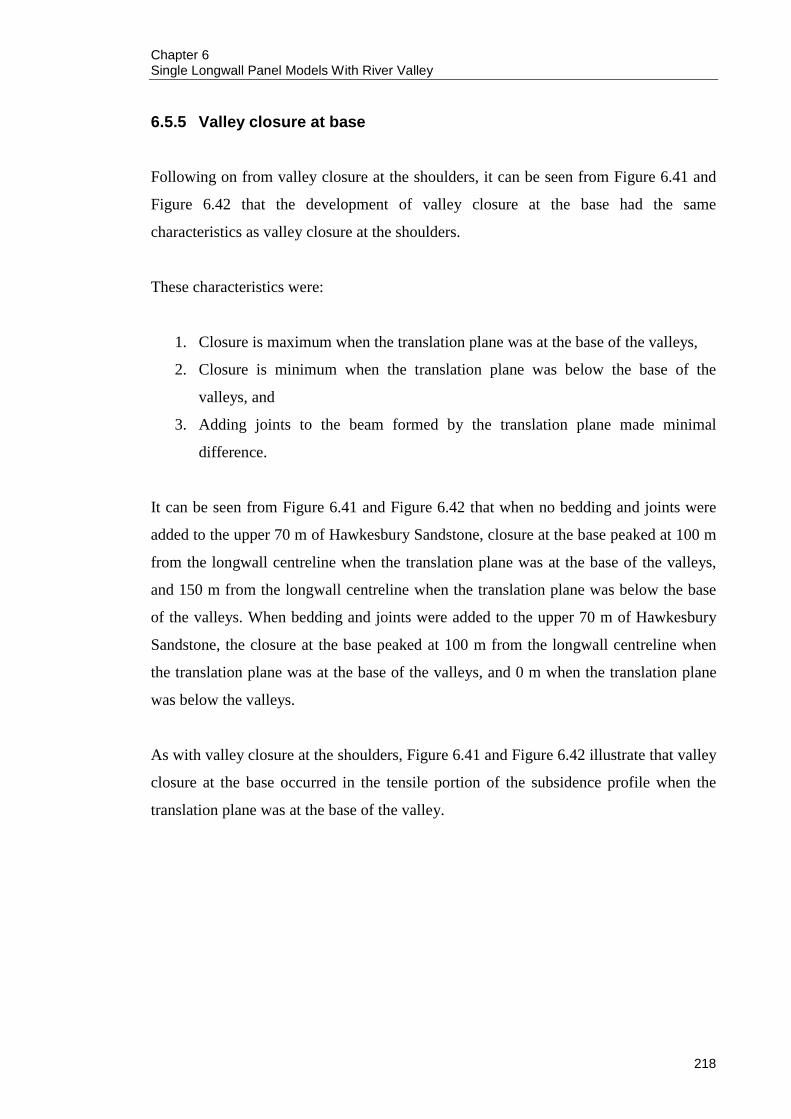
Chapter 6 Single Longwall Panel Models With River Valley
218
6.5.5 Valley closure at base
Following on from valley closure at the shoulders, it can be seen from Figure 6.41 and
Figure 6.42 that the development of valley closure at the base had the same
characteristics as valley closure at the shoulders.
These characteristics were:
1. Closure is maximum when the translation plane was at the base of the valleys,
2. Closure is minimum when the translation plane was below the base of the
valleys, and
3. Adding joints to the beam formed by the translation plane made minimal
difference.
It can be seen from Figure 6.41 and Figure 6.42 that when no bedding and joints were
added to the upper 70 m of Hawkesbury Sandstone, closure at the base peaked at 100 m
from the longwall centreline when the translation plane was at the base of the valleys,
and 150 m from the longwall centreline when the translation plane was below the base
of the valleys. When bedding and joints were added to the upper 70 m of Hawkesbury
Sandstone, the closure at the base peaked at 100 m from the longwall centreline when
the translation plane was at the base of the valleys, and 0 m when the translation plane
was below the valleys.
As with valley closure at the shoulders, Figure 6.41 and Figure 6.42 illustrate that valley
closure at the base occurred in the tensile portion of the subsidence profile when the
translation plane was at the base of the valley.
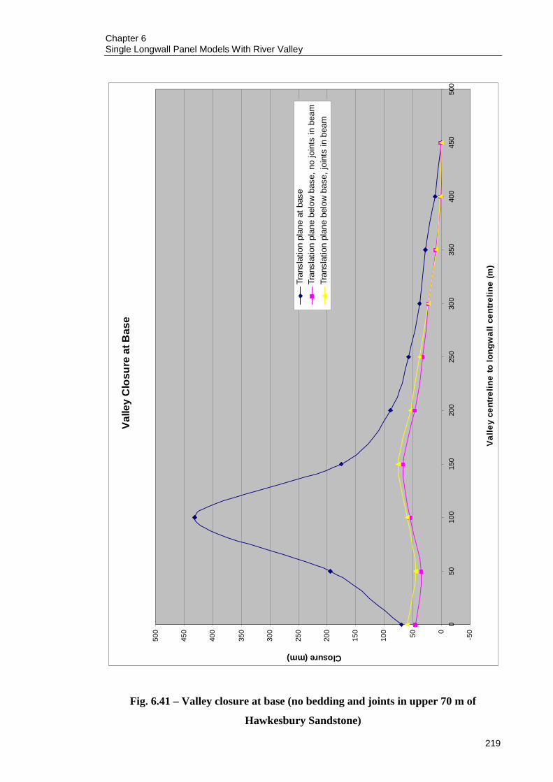
Chapter 6 Single Longwall Panel Models With River Valley
219
Fig. 6.41 – Valley closure at base (no bedding and joints in upper 70 m of
Hawkesbury Sandstone)
Valle
y C
losu
re a
t Bas
e
-50050100
150
200
250
300
350
400
450
500
050
100
150
200
250
300
350
400
450
500
Val
ley
cent
relin
e to
long
wal
l cen
trel
ine
(m)
Closure (mm)
Tran
slat
ion
plan
e at
bas
eTr
ansl
atio
n pl
ane
belo
w b
ase,
no
join
ts in
bea
mTr
ansl
atio
n pl
ane
belo
w b
ase,
join
ts in
bea
m
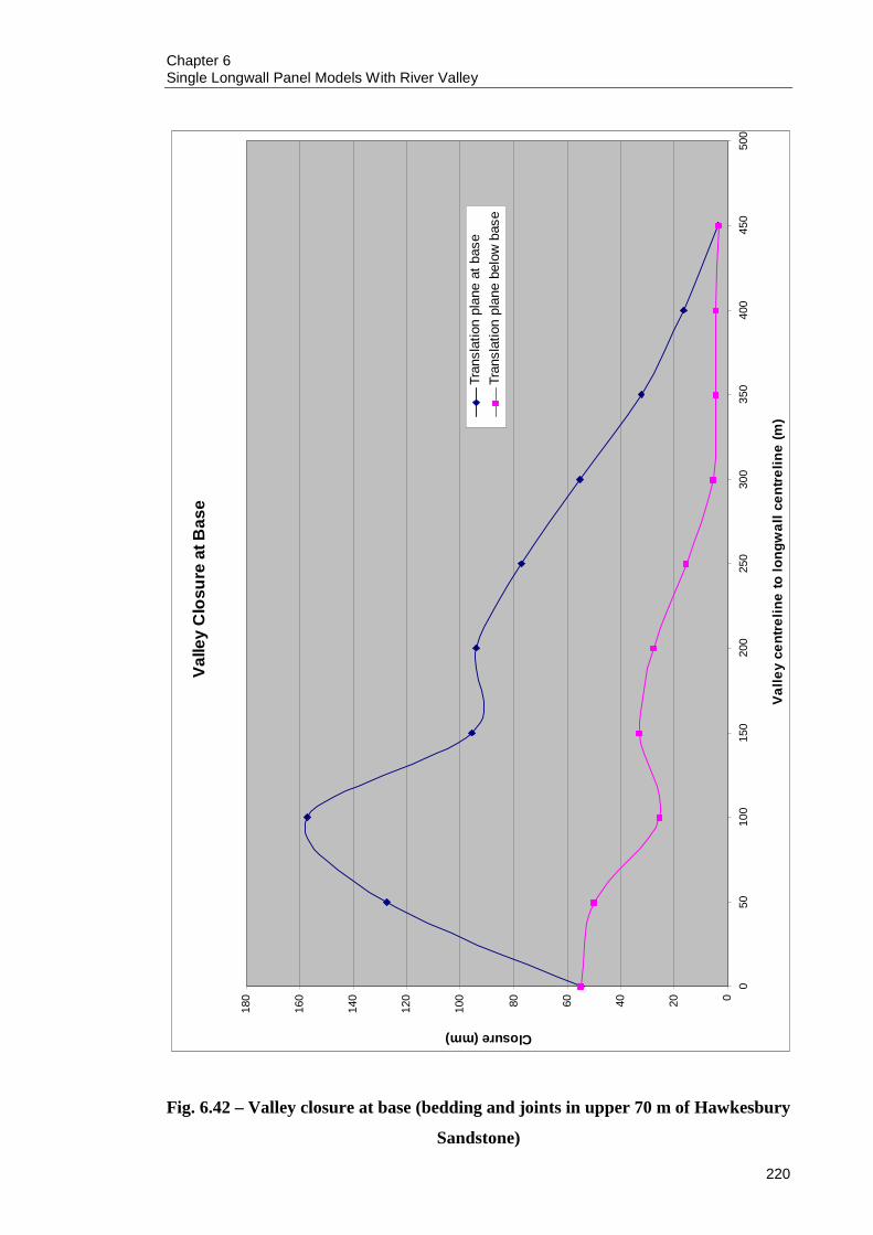
Chapter 6 Single Longwall Panel Models With River Valley
220
Fig. 6.42 – Valley closure at base (bedding and joints in upper 70 m of Hawkesbury
Sandstone)
Valle
y C
losu
re a
t Bas
e
020406080100
120
140
160
180
050
100
150
200
250
300
350
400
450
500
Val
ley
cent
relin
e to
long
wal
l cen
trel
ine
(m)
Closure (mm)
Tran
slat
ion
plan
e at
bas
eTr
ansl
atio
n pl
ane
belo
w b
ase

Chapter 6 Single Longwall Panel Models With River Valley
221
6.5.6 Valley base yield
The river valley models were examined for cases where yielded elements were present
in the base of the valleys.
The models that contained bedding and joints in the upper 70 m of the Hawkesbury
Sandstone did not contain any cases of yield in the valley bases when the translation
plane was at the base of the valleys. This was expected because the extra bedding and
joints in the walls of the valleys served to relieve any build up of horizontal stresses by
sliding out. When the translation plane was below the base of the valleys, upsidence and
beam buckling occurred, and the beam formed by the translation plane yielded when the
valley was above the longwall centreline, and gradually tapered off at 50 m from the
longwall centreline. Figure 6.43 is a plot of yield when the valley was directly above the
longwall centreline, and Figure 6.44 is a plot of yield when the valley was 50 m from
the longwall centreline.
The models that did not have any bedding and joints in the upper 70 m of the
Hawkesbury Sandstone exhibited yield in the valley bases, and this occurred only when
the translation plane was moved one metre below the base of the valleys. When the
beam formed by the translation plane contained no joints, the yield occurred in valleys
located directly above the longwall centreline, and out to 100 m from the longwall
centreline. When the beam formed by the translation plane contained joints, yield
occurred in valleys also up to 100 m longwall centreline. Figure 6.45 is a plot of yield
when the valley was directly above the longwall centreline, and Figure 6.46 is a plot of
yield when the valley was 100 m from the longwall centreline.
The increased occurrence of yield in the models without bedding and joints in the upper
70 m of Hawkesbury Sandstone implied that greater valley base yield occurred when
the sides of the valleys were represented as rigid blocks, and this was supported by the
rigid block movements observed by Holla and Barclay (2000).
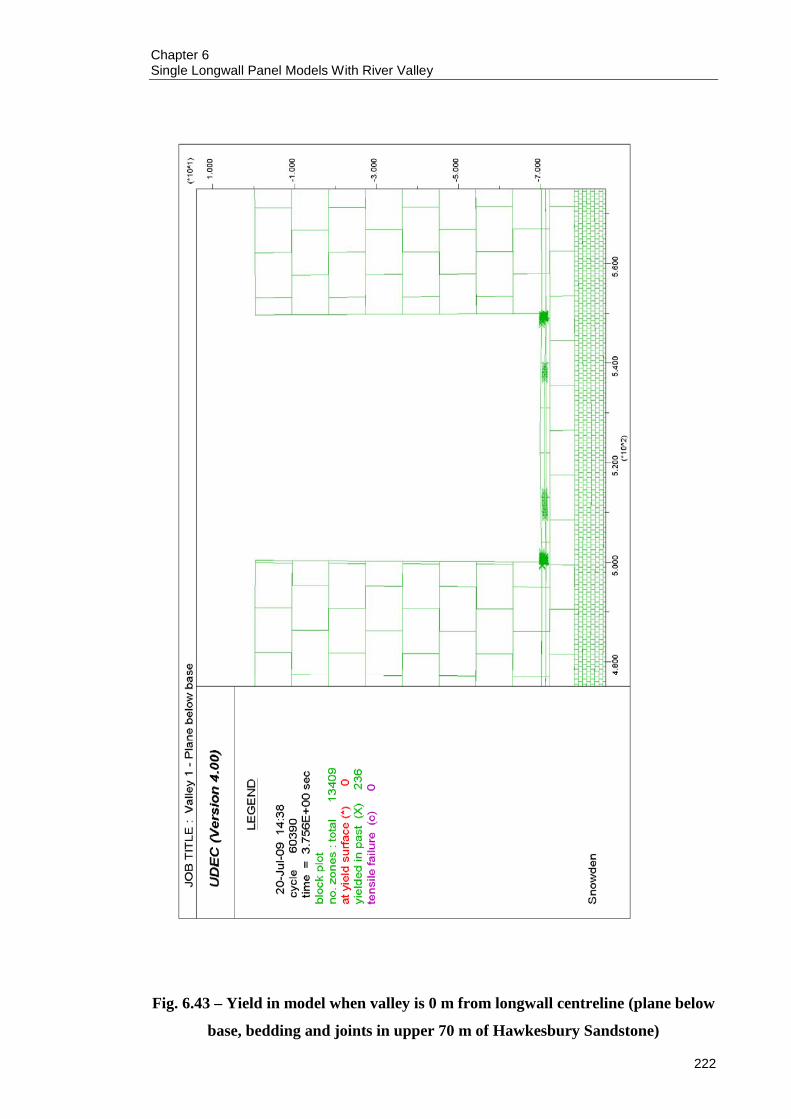
Chapter 6 Single Longwall Panel Models With River Valley
222
Fig. 6.43 – Yield in model when valley is 0 m from longwall centreline (plane below
base, bedding and joints in upper 70 m of Hawkesbury Sandstone)
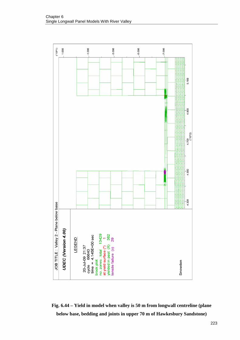
Chapter 6 Single Longwall Panel Models With River Valley
223
Fig. 6.44 – Yield in model when valley is 50 m from longwall centreline (plane
below base, bedding and joints in upper 70 m of Hawkesbury Sandstone)

Chapter 6 Single Longwall Panel Models With River Valley
224
Fig. 6.45 – Yield in model when valley is 0 m from longwall centreline (plane below
base, no bedding and joints in upper 70 m of Hawkesbury Sandstone)

Chapter 6 Single Longwall Panel Models With River Valley
225
Fig. 6.46 – Yield in model when valley is 100 m from longwall centreline (plane
below base, no bedding and joints in upper 70 m of Hawkesbury Sandstone)

Chapter 6 Single Longwall Panel Models With River Valley
226
6.6 COMPARISON TO EMPIRICAL DATA
The results from the models with no valley excavation indicated that average tilts
ranged from 3.89 mm/m to 4.90 mm/m, both being close to the average tilt of 4 mm/m
noted by Holla and Barclay (2000).
The closure results in Tables 6.4 to 6.8 are plotted (in red) against the empirical data
plots produced by Waddington Kay and Associates (2002) in Figures 6.47 to 6.56
respectively. The upsidence results in Tables 6.9 to 6.11 are plotted (in red) against
empirical data in Figures 6.57 to 6.59 respectively. It must be noted that not all values in
the above mentioned tables were able to be plotted, either because they exceeded the
maximum values on the empirical plots or they were negative (explained as boundary
effects earlier).
It can be seen from Figures 6.47 to 6.59 that there are observed data points (in blue) and
adjusted data points in the Waddington Kay and Associates database. From Figures 6.47
to 6.59 it is encouraging to note that the shoulder closure and upsidence results from the
river valley models mostly fall within the adjusted upper bound curve and closely
mirror the observed data points, instead of the adjusted data points. This suggests that
the shoulder closure and upsidence patterns produced by the models replicated the trend
observed in the empirical data.
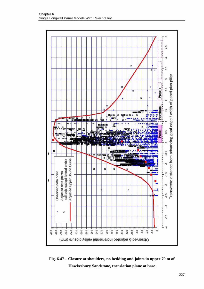
Chapter 6 Single Longwall Panel Models With River Valley
227
Fig. 6.47 – Closure at shoulders, no bedding and joints in upper 70 m of
Hawkesbury Sandstone, translation plane at base
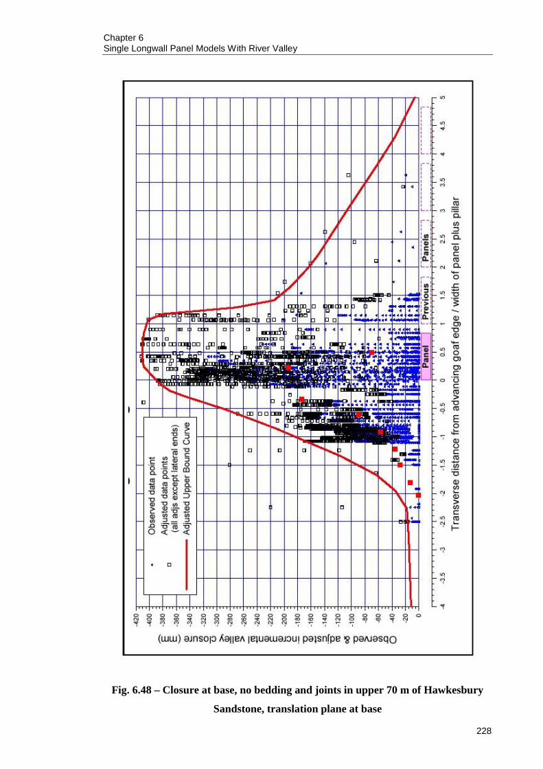
Chapter 6 Single Longwall Panel Models With River Valley
228
Fig. 6.48 – Closure at base, no bedding and joints in upper 70 m of Hawkesbury
Sandstone, translation plane at base

Chapter 6 Single Longwall Panel Models With River Valley
229
Fig. 6.49 – Closure at shoulders, no bedding and joints in upper 70 m of
Hawkesbury Sandstone, translation plane below base, no joints in beam

Chapter 6 Single Longwall Panel Models With River Valley
230
Fig. 6.50 – Closure at base, no bedding and joints in upper 70 m of Hawkesbury
Sandstone, translation plane below base, no joints in beam
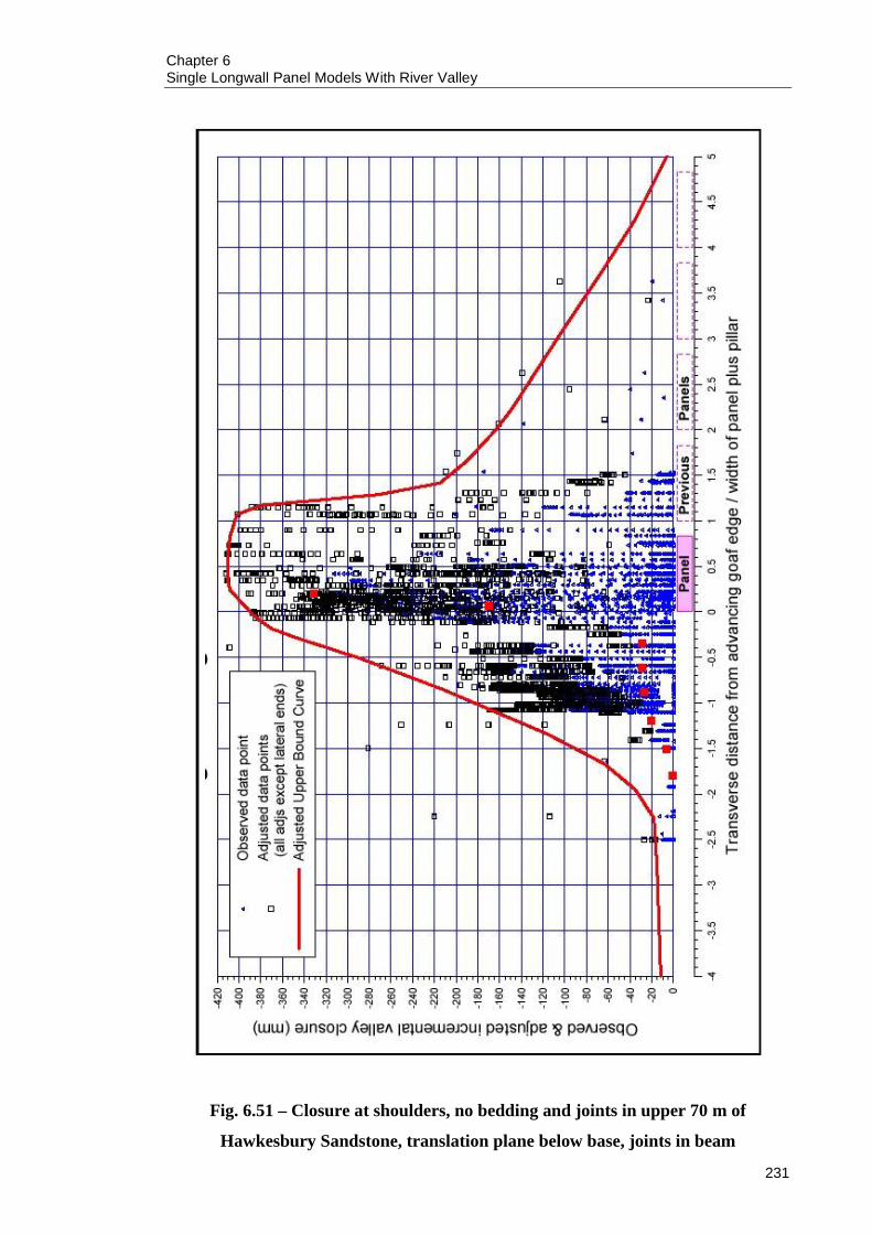
Chapter 6 Single Longwall Panel Models With River Valley
231
Fig. 6.51 – Closure at shoulders, no bedding and joints in upper 70 m of
Hawkesbury Sandstone, translation plane below base, joints in beam

Chapter 6 Single Longwall Panel Models With River Valley
232
Fig. 6.52 – Closure at base, no bedding and joints in upper 70 m of Hawkesbury
Sandstone, translation plane below base, joints in beam

Chapter 6 Single Longwall Panel Models With River Valley
233
Fig. 6.53 – Closure at shoulders, bedding and joints in upper 70 m of Hawkesbury
Sandstone, translation plane at base
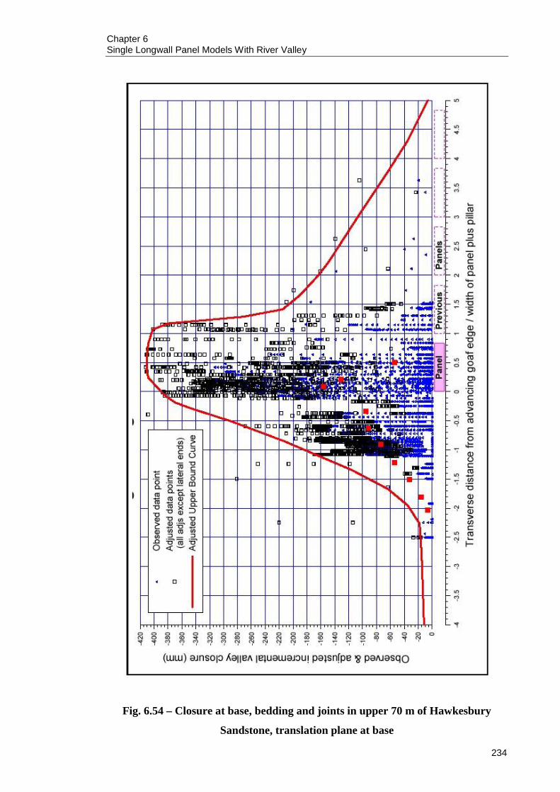
Chapter 6 Single Longwall Panel Models With River Valley
234
Fig. 6.54 – Closure at base, bedding and joints in upper 70 m of Hawkesbury
Sandstone, translation plane at base
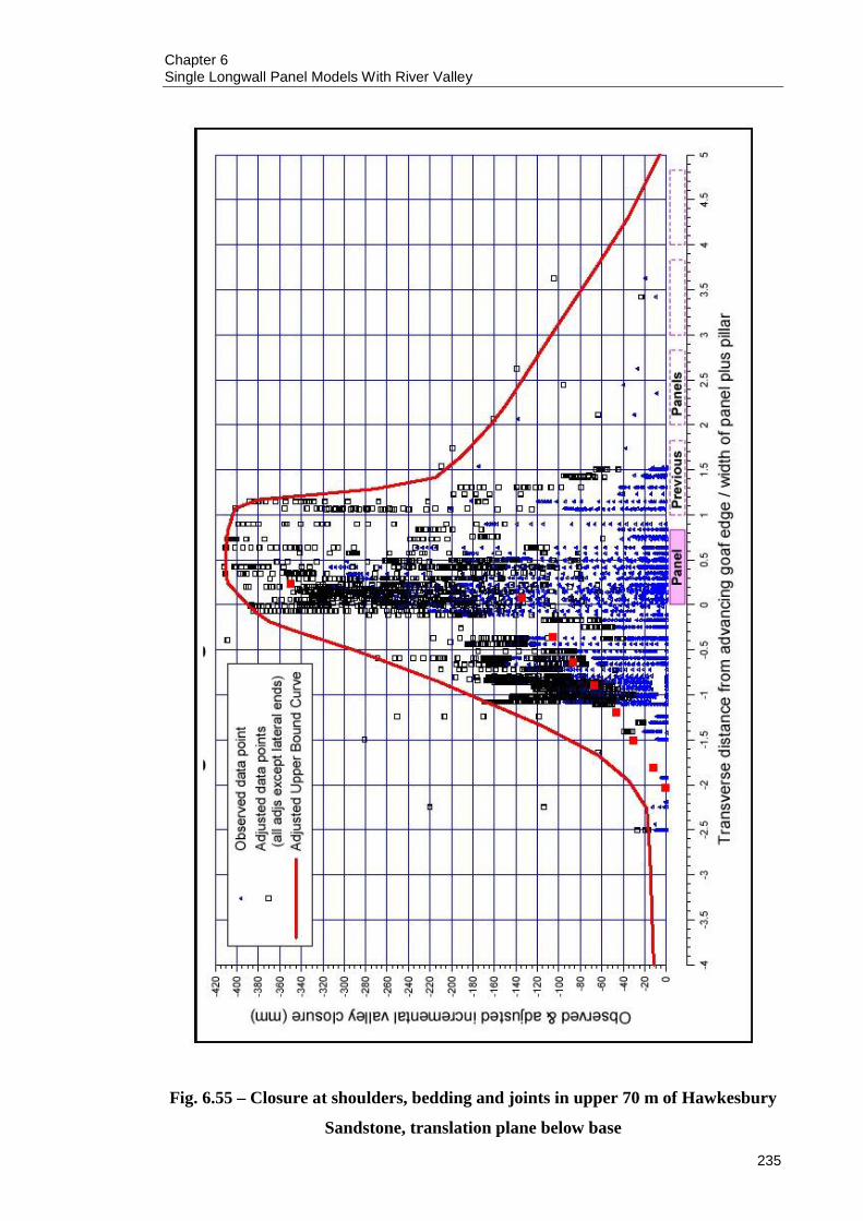
Chapter 6 Single Longwall Panel Models With River Valley
235
Fig. 6.55 – Closure at shoulders, bedding and joints in upper 70 m of Hawkesbury
Sandstone, translation plane below base

Chapter 6 Single Longwall Panel Models With River Valley
236
Fig. 6.56 – Closure at base, bedding and joints in upper 70 m of Hawkesbury
Sandstone, translation plane below base

Chapter 6 Single Longwall Panel Models With River Valley
237
Fig. 6.57 – Upsidence at base (from Table 6.9)

Chapter 6 Single Longwall Panel Models With River Valley
238
Fig. 6.58 – Upsidence at base (from Table 6.10)
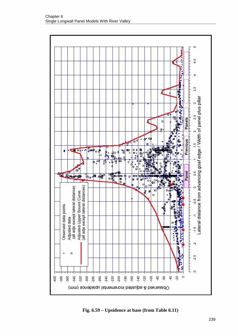
Chapter 6 Single Longwall Panel Models With River Valley
239
Fig. 6.59 – Upsidence at base (from Table 6.11)

Chapter 6 Single Longwall Panel Models With River Valley
240
6.7 PARAMETRIC STUDY
A parametric study was performed to examine the effect of the translation plane friction
angle and cohesion. Twenty five models were created that varied the friction angle from
20° to 40° and the cohesion from 2 MPa to 10 MPa. These models were based on the
river valley model that contained the valley centre 150 m from the longwall centreline
(Valley 4, see Table 6.4). The purpose of this parametric study was to gain an insight
into joint conditions (friction and cohesion) required to limit movement. Table 6.12 lists
the additional models and the results.
Table 6.12 – Additional models for parametric study and results
Model Joint Friction Angle (°)
Joint Cohesion (MPa)
Closure Top (mm)
Closure Bottom (mm)
1 20 2 74 177 2 20 4 76 177 3 20 6 65 157 4 20 8 9 18 5 20 10 9 17 6 25 2 73 177 7 25 4 76 157 8 25 6 9 17 9 25 8 9 17
10 25 10 9 17 11 30 2 73 177 12 30 4 77 177 13 30 6 9 17 14 30 8 9 17 15 30 10 9 17 16 35 2 75 177 17 35 4 76 177 18 35 6 9 17 19 35 8 9 17 20 35 10 9 16 21 40 2 77 177 22 40 4 9 17 23 40 6 9 17 24 40 8 9 17 25 40 10 9 17
The results in Table 6.12 can be seen in Figures 6.60 to 6.63.

Chapter 6 Single Longwall Panel Models With River Valley
241
Fig. 6.60 – Valley closure at top of valley as a function of joint friction angle
Val
ley
Clo
sure
at T
op o
f Val
ley
0102030405060708090
02
46
810
12
Join
t Coh
esio
n (M
Pa)
Closure (mm)
20 d
egre
es
25 d
egre
es
30 d
egre
es
35 d
egre
es
40 d
egre
es
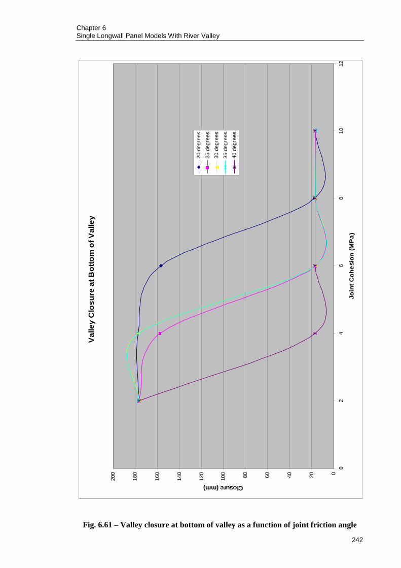
Chapter 6 Single Longwall Panel Models With River Valley
242
Fig. 6.61 – Valley closure at bottom of valley as a function of joint friction angle
Val
ley
Clo
sure
at B
otto
m o
f Val
ley
020406080100
120
140
160
180
200
02
46
810
12
Join
t Coh
esio
n (M
Pa)
Closure (mm)
20 d
egre
es
25 d
egre
es
30 d
egre
es
35 d
egre
es
40 d
egre
es
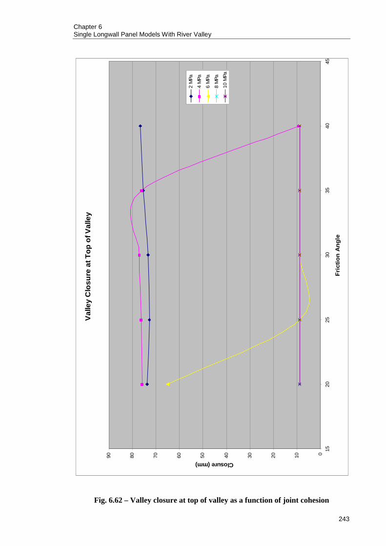
Chapter 6 Single Longwall Panel Models With River Valley
243
Fig. 6.62 – Valley closure at top of valley as a function of joint cohesion
Val
ley
Clo
sure
at T
op o
f Val
ley
0102030405060708090
1520
2530
3540
45
Fric
tion
Ang
le
Closure (mm)
2 M
Pa
4 M
Pa
6 M
Pa
8 M
Pa
10 M
Pa

Chapter 6 Single Longwall Panel Models With River Valley
244
Fig. 6.63 – Valley closure at bottom of valley as a function of joint cohesion
Val
ley
Clo
sure
at B
otto
m o
f Val
ley
020406080100
120
140
160
180
200
1520
2530
3540
45
Fric
tion
Ang
le
Closure (mm)
2 M
Pa
4 M
Pa
6 M
Pa
8 M
Pa
10 M
Pa
Chapter 6 Single Longwall Panel Models With River Valley
245
It can be seen from Figure 6.60 that as joint cohesion increased, valley closure
decreased. In all cases of joint friction angle, valley closure stabilised at 9 mm. When
the joint friction angle was 20°, the required joint cohesion to stabilise the closure was
8 MPa. When the joint friction angle was 25°, 30° and 35°, the required joint cohesion
was 6 MPa. When the joint friction angle was 40°, the required joint cohesion was
4 MPa. This was logical as it was expected that as joint friction angle increased, valley
closure would decrease, and likewise with joint cohesion (which was evident by the
decreasing amount of joint cohesion required to bring the closure down to the minimum
level as joint friction angle increased). The same behaviour is evident in Figure 6.61.
When the results are plotted as a function of joint cohesion, it can be seen from Figure
6.62 and Figure 6.63 that when the joint cohesion is 2 MPa, the closure does not reduce
to a minimum level throughout the range of joint friction angles. A joint cohesion of
4 MPa appeared to be the threshold at which the valley closure reduced dramatically as
joint friction angle increased, in this case 35°. As expected, as the joint cohesion
increased above 4 MPa, there was a reduction in the joint friction angle needed to bring
the valley closure to a minimum.
6.8 COMPARISON TO BLOCK KINEMATICS
It was discussed earlier in Chapter 3 that inward closure of the valley wall that is
furthest from the longwall panel, or the total valley closure of a valley directly above a
longwall panel could potentially be calculated by Equation 3.12, which essentially
related valley closure and tilt.
The inward shoulder closure of the valley walls furthest from the longwall panel was
calculated using Equation 3.12 and the results are in Table 6.13 and Figure 6.64. The
calculations have been performed on the models that have the translation plane at the
base of the valleys and no bedding and joints in the upper 70 m of Hawkesbury
Sandstone.
The valley closure at the shoulders for the valleys directly over the longwall centreline
was also calculated using Equation 3.12 and the results are in Table 6.14.

Chapter 6 Single Longwall Panel Models With River Valley
246
Table 6.13 – Valley wall closure comparison
Valley Valley centre to longwall centre (m)
Analytical valley wall closure (mm)
UDEC valley wall closure (mm)
1 0 381 375 2 50 104 133 3 100 14 20 4 150 9 14 5 200 7 9 6 250 4 6 7 300 3 4 8 350 0 2 9 400 1 1
10 450 0 0
Table 6.14 – Valley closure comparison
Model Analytical valley closure (mm)
UDEC valley closure (mm)
Translation plane at base 736 727 Translation plane below base, no joints in beam 724 708
Translation plane below base, joints in beam 719 701
It can be seen from Table 6.13 and Figure 6.64 that Equation 3.12 calculated valley wall
closure quite well. It can also be seen from Table 6.14 that Equation 3.12 calculated
total valley closure for valleys directly above the longwall centreline to within 2 % of
the values produced by UDEC.

Chapter 6 Single Longwall Panel Models With River Valley
247
Fig. 6.64 – Comparison of valley wall closure at shoulders between the UDEC
models and the block kinematic solution
Val
ley
Wal
l Clo
sure
at S
houl
ders
-50050100
150
200
250
300
350
400
050
100
150
200
250
300
350
400
450
500
Val
ley
cent
relin
e to
long
wal
l cen
trel
ine
(m)
Wall closure (mm)
UD
EC
Blo
ck k
inem
atic
sol
utio
n

Chapter 6 Single Longwall Panel Models With River Valley
248
6.9 SUMMARY
A series of simplified models that represented each potential river valley as a block was
constructed to test the alternative block movement theory. Two major cases (with
variations) were considered, the first where a translation plane existed at the base of the
valley and the second, where a translation plane existed one metre below the base of the
valley. The variations included adding bedding and joints in the upper 70 m of the
Hawkesbury Sandstone and adding vertical joints in the beam formed by the translation
plane one metre below the base of the valley. It was proposed that for the first case,
valley closure would be maximised whilst upsidence and valley base yield would be
minimised. For the second case, it was proposed that valley closure would decrease and
upsidence and valley base yield would increase due to the effect of the translation plane.
From the results it was seen that the models conformed to the proposed block
movement explanation. When the translation plane was located at the base of the valley,
the blocks closest to the longwall panel slid along the plane away from the longwall
panel and the blocks in the left hand side of the valley moved towards the longwall
panel as a function of the geometry of the subsidence profile (see Figure 6.35 and
Figure 6.40), maximising valley closure and minimising valley base yield. When the
translation plane was located one metre below the base of the valley, the blocks
exhibited similar behaviour but produced lesser valley closure whilst at the same time
increasing the occurrence of upsidence (see Figures 6.25 to 6.27), and valley base yield
as a result of the horizontal stress build up due to the lack of a sliding surface at the base
of the valleys (see Figures 6.43 to 6.46). The term yield instead of failure has been used
in the discussion of results as the UDEC models are quite simple.
The results from the numerical models were plotted against the empirical curves and it
was seen that most of the model data points were contained below the empirical upper-
bound curve and most of the model data points were situated within the observed
empirical data points (see Figures 6.47 to 6.59). This was fitting as the model data
points were not adjusted at all. This further supported the block movement theory, as
the models were based on the block movement theory and also conformed to observed
field behaviour (Holla & Barclay 2000).

Chapter 6 Single Longwall Panel Models With River Valley
249
The parametric study revealed that the magnitudes of closure at the top and bottom of
the valleys were quite sensitive to the range of joint cohesion (2 MPa, 4 MPa, 6 MPa,
8 MPa and 10 MPa) and joint friction angle (20°, 25°, 30°, 35° and 40°) modelled. The
parametric study also provided clues as to what the threshold values for joint friction
angle and joint cohesion was needed to drastically reduce closure at the top and bottom
of the valleys (see Figures 6.60 to 6.63). This concept could prove useful when
considering which method to use to strengthen the valley base prior to mining.
The model results were also compared to the block kinematics discussed in Chapter 3.
Using Equation 3.12, valley wall closure and total valley closure above the longwall
centreline was calculated and compared to the model results (see Table 6.13, Table 6.14
and Figure 6.64). The trends were captured quite well and could be the subject of
further refinement and investigation in the future.
In summary, the river valley models have successfully demonstrated the mechanism
behind the proposed block movement model, i.e. block sliding and valley closure occurs
with minimal upsidence when a translation plane exists at the base of the valley, and
increased upsidence and reduced valley closure occur when the translation plane is
below the base of the valley (see Figures 6.24, 6.29, 6.33, 6.34, 6.41 and 6.42).
Furthermore, the river valley models demonstrated that tilt dependant valley closure
was occurring at a distance several hundred metres away from the longwall centreline
(in the hogging or tensile portion of the subsidence profile), by virtue of blocks being
pushed into the void created by the valley (see Figures 6.36, 6.37 and 6.40). The end
result is a demonstrated mechanism that produces closure and identifies what can cause
the onset of upsidence. More importantly, it suggests that quantifying closure may be
possible.

Chapter 7 Application Of Voussoir Beam And Plate Buckling Theory
250
CHAPTER 7 APPLICATION OF VOUSSOIR BEAM AND PLATE
BUCKLING THEORY
7.1 INTRODUCTION
Independent checks on aspects of the numerical models that were introduced in Chapter
5 and Chapter 6 are the subject of consideration in this chapter. Voussoir beam theory
will be applied to the models developed in Chapter 5 to corroborate the ability of the
models in simulating the deflection of the Bulgo Sandstone, and plate buckling theory
will be applied to the models developed in Chapter 6 to corroborate the ability of the
models in predicting valley base yield.
7.2 APPLICATION OF VOUSSOIR BEAM THEORY
A basic derivation and how to use voussoir beam theory from Sofianos (1996), Sofianos
and Kapenis (1998) and Nomikos, Sofianos and Tsoutrelis (2002) can be found in
Appendix E. This theory has been used to calculate the theoretical deflection of the
Bulgo Sandstone in Models 1 to 4.
The results from Models 1 to 4 (Chapter 5) indicated that the Bulgo Sandstone was the
massive spanning unit in the overburden and the majority of the caving was confined
below the base of the massive unit. This was the case for Model 2, whilst failure
extended into the Bulgo Sandstone in Models 3 and 4. It was noted that caving was not
sufficient enough to produce any measurable goaf angle in Model 1, therefore this
model could not be analysed with the voussoir beam method. The geometry of the cave
zone was defined by a goaf angle of 11° to 25° for Model 2, 14° to 25° for Model 3 and
13° to 25° for Model 4.

Chapter 7 Application Of Voussoir Beam And Plate Buckling Theory
251
In order to perform an analysis, the following parameters must be known:
Longwall panel width (m),
Cover depth (m),
Hawkesbury Sandstone thickness (m),
Newport Formation thickness (m),
Bald Hill Claystone thickness (m),
Bald Hill Claystone density (kg/m3),
Bulgo Sandstone thickness (m),
Bulgo Sandstone density (kg/m3),
Bulgo Sandstone Young’s Modulus (MPa),
Cave zone height (m), and
Goaf angle (°).
See Figure 2.1 for a definition on caving height and goaf angle.
It is important to note that the analysis is actually performed on the base of the Bulgo
Sandstone as defined by the bedding plane spacing and extent of failure into the
spanning unit, and using the notion that thinner bedded layers load thicker bedded layers
(Obert & Duvall 1967), it is only the Bald Hill Claystone that acts as a surcharge on the
Bulgo Sandstone (see Table 5.5).
For example, if the Bulgo Sandstone is 92 m thick with a bedding plane spacing of 9 m,
the Bald Hill Claystone 12 m thick and the cave zone penetrates 64 m into the Bulgo
Sandstone, the analysis would be performed on the bottom 9 m of unbroken Bulgo
Sandstone with that layer being loaded by a surcharge of 31 m. The area and weight of
the surcharge was defined by the goaf angle and the weighted average density of the
surcharge. Using the procedure described in Appendix E, a simple spreadsheet was set
up to calculate the deflection of the Bulgo Sandstone for each model geometry. It was
found that the calculated deflections were highly sensitive to the goaf angle value.
However, there was agreement within the confines of the simple model for the goaf
angle. Table 7.1 contains the analytical and numerical deflection of the Bulgo
Sandstone.

Chapter 7 Application Of Voussoir Beam And Plate Buckling Theory
252
Table 7.1 – Analytical and numerical deflection of the Bulgo Sandstone
Model UDEC Deflection (mm)
UDEC Goaf Angle (°)
Back-Calculated Goaf Angle (°)
2 275 11 – 25 20.0 3 345 14 – 25 11.6 4 506 13 – 25 12.5
7.3 APPLICATION OF PLATE BUCKLING THEORY
The UDEC models in Chapter 6 produced behaviour that may indicate the onset of yield
in the base of the valleys of the type shown in Chapter 3. For the models that contained
the translation plane below the base of the valley, with no joints in the beam formed by
the translation plane, the maximum average horizontal stress immediately below the
sides of the valleys ranged from 18 MPa to 65 MPa.
Hoek and Brown (1980) provided a comprehensive overview of plate buckling theory,
and stated that the axial stress at which a plate will buckle is given by (Equation 7.1):
( )22
2
12 tlqEπσ α = [7.1]
Where,
σα = Axial stress required for buckling (MPa)
E = Elastic or Young’s Modulus (MPa)
q = A constant (0.5 for both ends clamped)
l = Length of plate (m)
t = Thickness of plate (m)
Equation 7.1 can be rearranged so that the critical thickness of a plate can be determined
if the axial stress is already known (Equation 7.2):
( )22 12qElt
ασπ= [7.2]
Chapter 7 Application Of Voussoir Beam And Plate Buckling Theory
253
Figure 7.1 illustrates the critical thickness for beams given an average horizontal stress
for different valley widths.
It can be seen from Figure 7.1 that when the values of maximum average horizontal
stresses in the river valley models (18 MPa – 65 MPa) are applied to this graph, the
calculated thickness of the beam that would buckle for a 50 m wide valley is in the
order of 1 m to 1.9 m. This is corroborated by the author’s recollection of buckling in a
similar geographical location where buckled slabs were usually 0.5 m to 1 m thick, and
rarely exceeded 2 m in thickness. Simple buckling (Figure 7.2) and low angle shear
(Figure 3.6) were common features in the field.
7.4 SUMMARY
Two analytical solutions were introduced and applied to the river valley numerical
models in an attempt to further test the credibility of the numerical models. This was
undertaken to provide a possible means of analysing a complex problem with simple
analytical tools and to assess whether there was any merit in using any of the solutions
in the future. It was seen that the numerical models complied with both analytical
solutions. Voussoir beam theory back-calculated goaf angles that were in general
agreement with the goaf angles produced by UDEC, and the plate buckling solution
(along with the author’s recollection of buckling events) suggested that the horizontal
stresses produced by the UDEC modelling is in the vicinity of what is required to
buckle the valley floor for the valley geometry modelled. The critical thickness of the
slabs calculated by the plate buckling analogue corresponds to field observations.
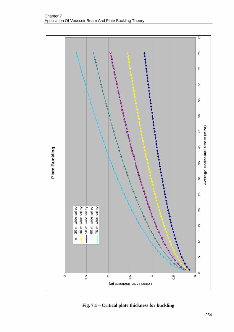
Chapter 7 Application Of Voussoir Beam And Plate Buckling Theory
254
Fig. 7.1 – Critical plate thickness for buckling
Pla
te B
uck
ling
0
0.51
1.52
2.53
05
1015
2025
3035
4045
5055
6065
7075
Ave
rag
e H
ori
zon
tal
Str
ess
(M
Pa
)
Critical Plate Thickness (m)
30 m
wid
e va
lley
40 m
wid
e va
lley
50 m
wid
e va
lley
60 m
wid
e va
lley
70 m
wid
e va
lley
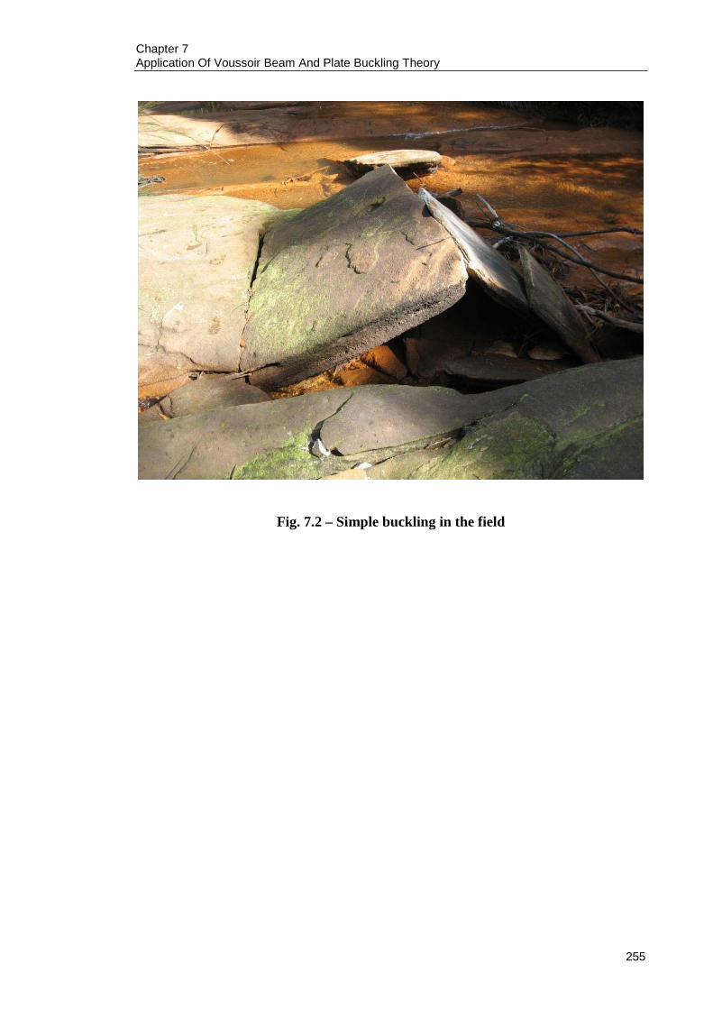
Chapter 7 Application Of Voussoir Beam And Plate Buckling Theory
255
Fig. 7.2 – Simple buckling in the field
Chapter 8 Summary, Conclusions And Recommendations
256
CHAPTER 8 SUMMARY, CONCLUSIONS AND
RECOMMENDATIONS
8.1 SUMMARY
This thesis aimed to investigate the mechanisms behind valley closure and upsidence
over unmined coal and old longwall panels using UDEC. In order to achieve this, the
choice of UDEC had to be justified and verified with the New South Wales Department
of Primary Industries empirical method of subsidence prediction (Holla & Barclay
2000), the empirical method developed by Waddington Kay and Associates (2002) for
valley closure and upsidence, and two analytical solutions.
One alternative explanation for valley closure and upsidence above unmined coal was
proposed and successfully investigated with UDEC.
This research has been driven by the need for understanding why valley closure and
upsidence occur above unmined coal, a phenomenon which can have far reaching
consequences in terms of surface damage and the possibility of forced sterilisation of
coal.
This project is a successful demonstration of the principles of using numerical,
empirical and analytical techniques to investigate a complex problem.
8.1.1 Review of problem
A review of valley closure and upsidence was undertaken and it was found that very
little literature exists on this topic. The most comprehensive review to date had been
performed by Waddington Kay & Associates (2002) and in this reference, a conceptual
model was proposed that suggested valley closure and upsidence is a result of some
undefined horizontal compressive stresses. It was speculated that this conceptual model
may be valid for river valleys that are directly undermined by longwall panels. The

Chapter 8 Summary, Conclusions And Recommendations
257
suggestion by Waddington Kay and Associates that upsidence is directly related to
valley closure was challenged.
The field data in Waddington Kay and Associates (2002) illustrated that valley closure
and upsidence was occurring above both unmined coal and old longwall panels
(Figure 3.8 and Figure 3.12), thereby raising questions about the wide application of this
horizontal compressive stress model, especially in areas above unmined coal that are
theoretically in tension and over old longwall panels which would have been relieved of
high horizontal compressive stresses during the extraction process.
Therefore, the questions that were raised about the horizontal compressive stress model
were:
1. Why does valley closure and upsidence occur in the tensile or hogging portion of the
subsidence profile above unmined coal?
2. Why does valley closure and upsidence occur over old longwall panels?
8.1.2 The block movement model To address the short-comings of the horizontal compressive stress model detailed in
Waddington Kay and Associates (2002) and to provide answers to the questions posed
above, an alternative model of block movements was proposed (Chapter 3).
The block movement model proposed that an incised ground surface is comprised of an
assemblage of blocks such that the valley incisions can be represented by the absence of
blocks. When the ground surface sags due to the extraction of a longwall panel, the
horizontal shortening of the ground surface above the longwall panel results in the
blocks being forced into the free face provided by the valley (Figure 3.17), whether it be
over unmined coal or old longwall panels.
This model assumed that the blocks had a surface to slide along, termed the translation
plane. If the translation plane existed at the bottom of the valley, then it was proposed
that valley closure would dominate over upsidence due to the dissipation in horizontal
stress provided by the translation plane. If the translation plane existed at a distance

Chapter 8 Summary, Conclusions And Recommendations
258
below the bottom of the valley, then it was proposed that valley closure would be
reduced and upsidence increased.
The kinematics of a particle moving along a curved surface was described and it was
pointed out that an adaptation to blocks moving along a curved surface was possible but
needed further investigation. It was deduced that the kinematics related horizontal
movement of the blocks to valley depth and curvature (Equation 3.12).
8.1.3 Numerical modelling The numerical modelling was undertaken in accordance to the guidelines set out in
Hudson, Stephansson and Andersson (2005). This was done to ensure that the modelling
process was fully traceable and transparent.
A review of recent references that dealt with UDEC, FLAC and similar software in
mining or underground applications was undertaken. It was found that whilst UDEC
seemed to be a more logical choice for modelling discontinuous rock masses, there was
a trend of using FLAC and creating custom constitutive models and calibrating material
properties. This approach is acceptable when a predictive model is required for a
localised area, but does not lend itself to a true predictor status. It was decided that
UDEC was the most appropriate software to use for this project because it did not
require the creation of a custom constitutive model or the excessive calibration of
material properties to replicate the effects of jointing.
The single longwall panel numerical models were created so they could be verified with
the empirical method. The geometry of the models and the model parameters were
derived from the literature. The models were designed to be transparent, and all the
model parameters and assumptions were fully traceable. It was also decided to make the
models as simple as possible to decrease the number of assumptions that had to be
made, as the more complex a numerical model is, the more uncertainty is built in. The
models were designed to predict maximum subsidence, goaf edge subsidence, strain, tilt
and inflection point location.

Chapter 8 Summary, Conclusions And Recommendations
259
When the models were analysed, it was seen that a goaf angle does exist and that the
caving was largely contained below the Bulgo Sandstone. This was in good agreement
with the factors identified in the literature survey on mine subsidence. When the results
were compared to the empirical curves (see Figures 5.8 to 5.13), it was seen that the
numerical predictions were in good agreement with the empirical curves. The only
parameter where the numerical predictions showed some limitations was the strain
predictions. This was attributed to the small levels of strain predicted and the inability
of the numerical model to predict strain of such small magnitude.
After the success of the single longwall panel models, a series of models were created to
simulate river valley response to mining in order to test if the proposed block movement
theory in Chapter 3 was plausible. Instead of creating a full scale model that
encompassed everything between the longwall and the surface, it was decided to scale
the model down by replicating the surface profile with a sequence of vertical
displacements that were applied to the new base of the model.
The new base of the model was determined by analysing the vertical displacements of
the surface, the Bald Hill Claystone and the Bulgo Sandstone. It was found that the
vertical displacement of the Bald Hill Claystone differed little from the surface vertical
displacements. When the Bald Hill Claystone was used as the base of the model, the
chance of yielded elements occurring in the vicinity of the river valley was too great to
ignore. As a result of this the Bulgo Sandstone was used as the base of the models,
thereby restricting yielded elements to those directly related to valley base yield, and not
those that were a by-product of the modelling procedure. All material and joint
properties remained the same as in the single longwall panel models to maintain
consistency.
Two types of models were developed. The first type incorporated a translation plane at
the base of the valleys and the second type incorporated a translation plane located one
metre below the base of the valleys. The purpose of this was to test the proposed block
movement theory in Chapter 3. It was noted that there was some uncertainty with the
exact definition of upsidence, and it was decided that for the purpose of the modelling,
upsidence was defined as the difference in upsidence between models with the
translation plane at the base of the valleys, and the models with the translation plane
Chapter 8 Summary, Conclusions And Recommendations
260
below the base of the valleys. Several variations were included in the numerical
modelling, including adding bedding and joints in the upper 70 m of the Hawkesbury
Sandstone, and adding joints to the beam formed by the translation plane.
The models behaved according to the proposed block movement theory and compared
well to the empirical and field observations (see Figures 6.20 to 6.59). The modelling
also demonstrated that tilt/curvature was the primary driver of valley closure and
upsidence, and was not controlled by a redistribution of horizontal stresses as widely
thought. A parametric study was conducted on the translation plane cohesion and
friction angle (see Figures 6.60 to 6.63), and it was found that it was possible to
quantify a joint cohesion and friction angle that was required to limit movement along
the translation plane.
The key objective of the numerical modelling was to demonstrate the block movement
model, a goal that has been achieved.
8.1.4 Application of analytical solutions
In an attempt to further the credibility of the numerical models, it was decided to apply
the voussoir beam solution to the single longwall panel models and the plate buckling
solution to the river valley models to see if the models corresponded with proven
analytical solutions. From the results it was seen that the voussoir beam solution back
calculated the goaf angle satisfactorily (see Table 7.1) and the plate buckling solution
corroborated with field observations (see Figure 7.1 and Figure 7.2). Both types of
models agreed well with the analytical solutions, even though the analytical solutions
were derived for elastic material.
8.2 CONCLUSIONS The following conclusions were drawn from this research project:
UDEC was suitable for use in mine subsidence related problems. This was
illustrated by the excellent match to the empirical curves used for validation
purposes. As UDEC is a Distinct Element code, the inclusion of joints

Chapter 8 Summary, Conclusions And Recommendations
261
automatically accounted for the reduction in rock mass strength, therefore
eliminating the need to modify or calibrate material properties derived by
laboratory testing. This is keeping in accordance with the transparent and fully
traceable principle.
The block movement model was a feasible explanation for valley closure above
unmined coal and old longwall panels. The numerical modelling demonstrated
that the forces generated were sufficient to induce movement in the hogging
portion of the subsidence profile by forcing blocks in an outward direction into
the void provided by the valley. In addition, the kinematics was relatively simple
and explained the relationship between block movement, valley depth and
tilt/curvature.
The block movement model was capable of indicating the onset of valley base
yield. This was extensively demonstrated in the numerical modelling.
The block movement model also introduced a number of implications. Block
rotations on a curved surface may induce surface cracking that extends to the
depth of the adjacent block, in any case much deeper than might be expected.
The depth of this surface cracking coupled with bedding plane dilation may have
adverse effects on horizontal permeability as well. It may be possible to control
the magnitude of upsidence or valley closure by reinforcing the valley base in
critical situations.
The block movement model demonstrated that it was possible to predict valley
closure and the onset of valley base yield using block kinematics and the plate
buckling solution. Further refinement is needed to replace numerical models
with analytical solutions; nevertheless the basic principles are sound.
8.3 LIMITATIONS OF THE STUDY
Modelling longwall caving, subsequent subsidence and river valley response is complex
and required simplifications and assumptions. The modelling work was limited by the
following conditions:
No three dimensional modelling was undertaken. Given the amount of unknown
assumptions that would have had to be made, limiting the modelling to two
dimensions was prudent.

Chapter 8 Summary, Conclusions And Recommendations
262
The difficulty in replication pillar deformation restricted the modelling to single
panel longwalls.
Some material properties from the geotechnical characterisation (MacGregor &
Conquest 2005) were missing and had to be evaluated using the Mohr-Coulomb
failure criteria and various guides.
Joint properties were not available and had to be assumed.
Vertical joint spacing was impossible to determine from core samples and was
assumed to be the same as bedding plane spacing.
Reproducing bulking in the goaf was difficult. Again, time constraints prevented
additional models being created with more random sub-vertical joint orientations
to try and increase bulking.
No field data was provided in order to verify models, the empirical method was
used for verification instead and this in itself was not ideal due to the data scatter
evident in the empirical curves.
8.4 RECOMMENDATIONS
This project achieved its objectives and it also highlighted areas that would benefit from
future research. These areas are:
The application of UDEC as a greenfields subsidence prediction tool in sub-
critical mining environments. This project has demonstrated that UDEC is
capable of predicting subsidence for single isolated panels provided that the
material properties are known.
The establishment of a geotechnical database containing typical rock mass and
joint properties for the rock units in the Southern Coalfield. Compiling the data
needed for the numerical modelling was one of the most time consuming
processes in the entire project.
It would be advantageous to model a wider range of longwall panel geometries
to try and cover the majority of the empirical prediction curve. For this to occur,
bulking needs to be replicated in the goaf to correctly model the large increase in
subsidence evident when W/H ratios exceed approximately 0.5.
In order to model multiple longwall panel layouts, further investigation into the
mechanics and numerical modelling of pillar deformation should be undertaken.

Chapter 8 Summary, Conclusions And Recommendations
263
Valley closure could theoretically be evaluated using block kinematics. Further
research needs to be carried out to derive expressions to calculate the forces
exerted by one block to another, and therefore displacement as the blocks
undergo rotation due to the development of the subsidence trough.

List Of References
264
LIST OF REFERENCES
1. Alehossein, H & Carter, J P 1990, ‘On the implicit and explicit inclusion of
joints in the analysis of rock masses’, in Rossmanith, H P (ed.), Proceedings of
the International Conference on Mechanics of Jointed and Faulted Rock, 18th –
20th April 1990, Institute of Mechanics, Technical University of Vienna,
Balkema, Rotterdam, pp. 487 – 494.
2. Alejano, L R, Ramirez-Oyanguren, P & Taboada, J 1999, ‘FDM predictive
methodology for subsidence due to flat and inclined coal seam mining’,
International Journal of Rock Mechanics and Mining Sciences, vol. 36, issue 4,
June 1999, pp. 475 – 491.
3. Australian Mining Engineering Consultants 2000, ‘The influence of subsidence
cracking on longwall extraction beneath water courses, aquifers, open cut voids
and spoil piles’, ACARP Research Project No. C5016, Australian Coal
Association Research Program, Brisbane, Queensland, Australia.
4. Badelow, F, Best, R, Bertuzzi, R & Maconochie, D 2005, ‘Modelling of defect
and rock bolt behaviour in geotechnical numerical analysis for Lane Cove
Tunnel’, Proceedings Geotechnical Aspects of Tunnelling for Infrastructure
Projects, Mini-Symposium, 12th October 2005, Milsons Point, Australia, 9 p.
5. Barton, N 1976, ‘The shear strength of rock and rock joints’, International
Journal of Rock Mechanics and Mining Sciences and Geomechanics Abstracts,
vol. 13, issue 9, September 1976, pp. 255 – 279.
6. Bhasin, R & Høeg, K 1998, ‘Parametric study for a large cavern in jointed rock
using a distinct element model (UDEC-BB)’, International Journal of Rock
Mechanics and Mining Sciences, vol. 35, issue 1, January 1998, pp. 17 – 29.

List Of References
265
7. BHP Billiton 2005, BHP Sustainability Report 2005 – Community Case Studies
– Integrated Mine Planning in the Illawarra, BHP Billiton, Melbourne, Victoria,
viewed 12 January 2007,
<http://hsecreport.bhpbilliton.com/2005/repository/community/caseStudies/case
Studies23.asp>.
8. Bowman, H N 1974, ‘Geology of the Wollongong, Kiama and Robertson
1:50,000 Sheets’, Geological Survey of New South Wales, Sydney.
9. Brady, B H & Brown, E T 2006, Rock Mechanics for Underground Mining, 3rd
edn, Springer, pp. 130 – 138.
10. Brady, B H, Hsiung, S H, Chowdhury, A H & Philip, J 1990, ‘Verification
studies on the UDEC computational model of jointed rock’, in Rossmanith, H P
(ed.), Proceedings of the International Conference on Mechanics of Jointed and
Faulted Rock, 18th – 20th April 1990, Institute of Mechanics, Technical
University of Vienna, Balkema, Rotterdam, pp. 551 – 558.
11. Chan, K F, Kotze, G P & Stone, P C 2005, ‘Geotechnical modelling of station
caverns for the Epping to Chatswood rail line project’, Proceedings
Geotechnical Aspects of Tunnelling for Infrastructure Projects, Mini-
Symposium, 12th October 2005, Milsons Point, Australia, 15 p.
12. Choi, S K & Coulthard, M A 1990, ‘Modelling of jointed rock masses using the
distinct element method’, in Rossmanith, H P (ed.), Proceedings of the
International Conference on Mechanics of Jointed and Faulted Rock, 18th – 20th
April 1990, Institute of Mechanics, Technical University of Vienna, Balkema,
Rotterdam, pp. 471 – 477.
13. Colwell Geotechnical Services 1998, ‘Chain pillar design (calibration of
ALPS)’, ACARP Research Project No. C6036, Australian Coal Association
Research Program, Brisbane, Queensland, Australia.

List Of References
266
14. Coulthard, M A 1995, ‘Distinct element modelling of mining-induced
subsidence – a case study’, in Myer, L R et al. (eds.), Proceedings of the
Conference on Fractured and Jointed Rock Masses, 3rd – 5th June 1992, Lake
Tahoe, California, USA, Balkema, Rotterdam, pp. 725 – 732.
15. Coulthard, M A & Dutton, A J 1988, ‘Numerical modelling of subsidence
induced by underground coal mining’ in Cundall P A, Sterling R L & Starfield,
A M (eds.), Proceedings of the 29th U.S. Symposium: Key Questions in Rock
Mechanics, 13th – 15th June 1988, University of Minnesota, Minneapolis,
Balkema, Rotterdam, pp. 529 – 536.
16. CSIRO Exploration & Mining & Strata Control Technology 1999, ‘Ground
behaviour about longwall faces and its effect on mining’, ACARP Research
Project No. C5017, Australian Coal Association Research Program, Brisbane,
Queensland, Australia.
17. CSIRO Petroleum 2002, ‘Numerical Modelling Studies’, in Waddington Kay &
Associates, ‘Research into the impacts of mine subsidence on the strata and
hydrology of river valleys and development of management guidelines for
undermining cliffs, gorges and river systems’, ACARP Research Project No.
C9067, Australian Coal Association Research Program, Brisbane, Queensland,
Australia.
18. Cundall, P A 1971, ‘A computer model for simulating progressive large-scale
movements in blocky rock systems’, Proceedings of the Symposium of the
International Society for Rock Mechanics, Nancy, France, 1971, vol. 1, Paper
No. II-8.
19. Gale, W J 2005, ‘Application of computer modelling in the understanding of
caving and induced hydraulic conductivity about longwall panels’, Proceedings
of the Coal2005 6th Australasian Coal Operators’ Conference, 26th – 28th April
2005, Brisbane, Australia, pp. 11 – 15.

List Of References
267
20. Ghobadi, M H 1994, ‘Engineering geologic factors influencing the stability of
slopes in the Northern Illawarra region’, PhD thesis, University of Wollongong,
Australia.
21. Hanlon, F N 1953, ‘Southern Coalfield, geology of the Stanwell Park – Coledale
area’, Technical Report No. 1, Department of Mines, New South Wales, pp. 20 –
35.
22. Hibbeler, RC 1997, Engineering Mechanics – Dynamics, SI edn, Prentice Hall,
pp. 47 – 49.
23. Hoek, E 2000, Rock Engineering Course Notes, Evert Hoek Consulting
Engineer Inc., viewed 7 March 2007,
<http://www.rocscience.com/hoek/PracticalRockEngineering.asp>.
24. Hoek, E & Brown, ET 1980, Underground Excavations in Rock, The Institute of
Mining and Metallurgy, p. 235.
25. Holla, L 1985, Mining Subsidence in New South Wales – Surface Subsidence
Prediction in the Southern Coalfield, New South Wales Department of Mineral
Resources, Sydney, p. 8.
26. Holla, L & Armstrong, M 1986, ‘Measurement of sub-surface strata movement
by multi-wire borehole instrumentation’, The AusIMM Bulletin & Proceedings,
The Australasian Institute of Mining and Metallurgy, Parkville, Victoria, vol.
291, no. 7, October 1986, pp. 65 – 72.
27. Holla, L & Barclay, E 2000, Mine Subsidence in the Southern Coalfield, NSW,
Australia, New South Wales Department of Mineral Resources, pp. 1 – 16.
28. Hudson, J A, Stephansson, O & Andersson, J 2005, ‘Guidance on numerical
modelling of thermo-hydro-mechanical coupled processes for performance
assessment of radioactive waste repositories’, International Journal of Rock
Mechanics and Mining Sciences, vol. 42, issues 5 – 6, July – September 1999,
pp. 850 – 870.

List Of References
268
29. Itasca 2000, UDEC User’s Guide Version 3.1, Itasca Consulting Group, Inc:
Minneapolis, Minnesota, USA.
30. Johansson, E, Reikkola, R & Lorig, L 1988, ‘Design analysis of multiple parallel
caverns using explicit finite difference methods’ in Cundall P A, Sterling R L &
Starfield, A M (eds.), Proceedings of the 29th U.S. Symposium: Key Questions in
Rock Mechanics, 13th – 15th June 1988, University of Minnesota, Minneapolis,
Balkema, Rotterdam, pp. 325 – 333.
31. Jones, B G & Rust, B R 1983, ‘Massive sandstone facies in the Hawkesbury
Sandstone, a Triassic fluvial deposit near Sydney, Australia’, Journal of
Sedimentary Research, vol. 53, no. 4, December 1983, pp. 1249 – 1259.
32. Kapp, W A 1984, ‘Mine subsidence and strata control in the Newcastle District
of the Northern Coalfield New South Wales’, PhD thesis, University of
Wollongong, Australia.
33. Kratzsch, H 1983, Mining Subsidence Engineering, Springer – Verlag, p. 41,
153.
34. MacGregor, S & Conquest, G 2005, ‘Geotechnical characterization and borehole
completion logs for surface boreholes: Endeavour 3 (WCC DDH29), Endeavour
4 (WCC DDH 30) and Endeavour 5 (WCC DDH 31)’, Report No. BHPC2843,
SCT Operations Pty. Ltd.
35. Mandl, G 2005, Rock Joints – The Mechanical Genesis, Springer – Verlag,
Germany, pp. 55 – 97.
36. McNally, G H 1996, ‘Estimation of the geomechanical properties of coal
measures rocks for numerical modelling’, in McNally, G M & Ward, C R (eds.),
Proceedings of the Symposium on Geology in Longwall Mining, 12th – 13th
November 1996, University of New South Wales, pp. 63 – 72.
List Of References
269
37. Mills, K W 2002, ‘In situ measurements and installation of monitoring
instruments at WRS1’, Report No. MET2367, Strata Control Technology
Operations Pty. Ltd., pp. 6 – 16.
38. Mills, K W & Huuskes, W 2004, ‘The effects of mining subsidence on rockbars
in the Waratah Rivulet at Metropolitan Colliery’, Proceedings of the 6th
Triennial Conference on Subsidence Management Issues, Mine Subsidence
Technological Society, Newcastle, Australia, pp. 47 – 64.
39. Mineral Policy Institute 2005, RIVERS SOS: BHP Billiton and others urged to
commit to mine a safe distance from precious water resources, Mineral Policy
Institute, Erskineville, New South Wales, viewed 12 January 2007,
<http://www.mpi.org.au/companies/bhpb/river_sos/>.
40. National Coal Board 1975, Subsidence Engineers’ Handbook, 2nd edn, National
Coal Board Mining Department, UK, 111 p.
41. Nemcik, J A 2003, ‘Floor failure mechanisms at underground longwall face’,
PhD thesis, University of Wollongong, Australia.
42. Nomikos, P P, Sofianos, A I & Tsoutrelis, C E 2002, ‘Structural response of
vertically multi-jointed roof rock beams’, International Journal of Rock
Mechanics and Mining Sciences, vol. 39, issue 1, January 2002, pp. 79 – 94.
43. NSW Department of Planning 2008, ‘Impacts of underground coal mining on
natural features in the Southern Coalfield – Strategic Review’, NSW Department
of Planning, Sydney.
44. NSW Planning Assessment Commission 2009, ‘The Metropolitan Coal Project –
Report Review’, NSW Planning Assessment Commission, Sydney.
45. Obert, L & Duvall, W I 1967, Rock Mechanics and the Design of Structures in
Rock, John Wiley and Sons, Inc., pp. 518 – 522.

List Of References
270
46. O’Connor, K M & Dowding, C H 1990, ‘Monitoring and simulation of mining-
induced subsidence’, in Rossmanith, H P (ed.), Proceedings of the International
Conference on Mechanics of Jointed and Faulted Rock, 18th – 20th April 1990,
Institute of Mechanics, Technical University of Vienna, Balkema, Rotterdam,
pp. 781 – 787.
47. Packham, G H (ed.) 1969, The Geology of New South Wales, The Geological
Society of Australia Incorporated, Sydney, pp. 370 – 375.
48. Pells, P J N 1985, ‘Engineering properties of rocks in the Narrabeen Group’, in
P J N Pells (ed.), Engineering Geology of the Sydney Region, Balkema,
Rotterdam, pp. 205 – 211.
49. Pells, P J N 1993, ‘The 1993 E.H Davies Memorial lecture, rock mechanics and
engineering geology in the design of underground works’, Australian
Geomechanics Society, pp. 3.1 – 3.33.
50. Peng, S S 1992, Surface Subsidence Engineering, Society for Mining,
Metallurgy, and Exploration, Inc. (AIME), Braun-Brumfield, Inc., pp. 1 – 20.
51. Price, N J 1966, Fault and Joint Development in Brittle and Semi-Brittle Rock,
Permagon Press Ltd., London, pp. 144 – 147.
52. Reynolds, R G 1977, ‘Coal mining under stored waters (stored waters inquiry
report)’, New South Wales Government, Sydney.
53. Seedsman, R W 2004, ‘Back analysis of sub-critical subsidence events in the
Newcastle Coalfield using voussoir beam concepts’, Proceedings of the 6th
Triennial Conference on Subsidence Management Issues, Mine Subsidence
Technological Society, Newcastle, Australia, pp. 65 – 74.
54. Selley, R C 2000, Applied Sedimentology, 2nd edn, Academic Press, California,
p. 142.

List Of References
271
55. Sitharam, T G & Madhavi Latha, G 2002, ‘Simulation of excavations in jointed
rock masses using a practical equivalent continuum approach’, International
Journal of Rock Mechanics and Mining Sciences, vol. 39, issue 4, June 2002, pp.
517 – 525.
56. Sofianos, A I 1996, ‘Analysis and design of an underground hard rock voussoir
beam roof’, International Journal of Rock Mechanics and Mining Sciences, vol.
33, issue 2, February 1996, pp. 153 – 166.
57. Sofianos, A I & Kapenis, A P 1998, ‘Numerical evaluation of the response in
bending of an underground hard rock voussoir beam roof’, International Journal
of Rock Mechanics and Mining Sciences, vol. 35, issue 8, December 1998, pp.
1071 – 1086.
58. Tucker, M E 2003, Sedimentary Rocks in the Field, 3rd edn, John Wiley & Sons
Ltd, England, pp. 88 – 94.
59. Waddington, A A & Kay, D R 1995, ‘The Incremental Profile Method for
prediction of subsidence, tilt, curvature and strain over a series of longwalls’,
Proceedings of the 3rd Triennial Conference on Mine Subsidence, Mine
Subsidence Technological Society, Newcastle, Australia, pp. 189 – 198.
60. Waddington, A A & Kay, D R 2001, ‘Closure and uplift in creeks, valleys and
gorges due to mine subsidence’, Proceedings of the 5th Triennial Conference on
Coal Mine Subsidence Current Practice and Issues, Mine Subsidence
Technological Society, Newcastle, Australia, pp. 49 – 61.
61. Waddington Kay & Associates 2002, ‘Research into the impacts of mine
subsidence on the strata and hydrology of river valleys and development of
management guidelines for undermining cliffs, gorges and river systems’,
ACARP Research Project No. C9067, Australian Coal Association Research
Program, Brisbane, Queensland, Australia.
List Of References
272
62. Waddington Kay & Associates, CSIRO Petroleum Division & University of
New South Wales 2002, ‘Management information handbook on the
undermining of cliffs, gorges and river systems – projects C8005 and C9067’,
Australian Coal Association Research Program, Brisbane, Queensland,
Australia.
63. Whittaker, B N & Reddish, D J 1989, Subsidence – Occurrence, Prediction and
Control, Elsevier Science Publishers B V, pp. 15 – 113.
64. Williams, W A & Gray, P A 1980, ‘The nature and properties of coal and coal
measure strata’, in Hargraves, A J (ed.), Proceedings of Support in Coal Mines,
The Aus. I.M.M., Illawarra Branch Roof Support Colloquium, September 1980,
The Australasian Institute of Mining and Metallurgy, Parkville, Victoria,
Australia, pp. 1 – 12.

Appendix A Numerical Modelling Audits
273
APPENDIX A NUMERICAL MODELLING AUDITS
A.1 PART 1 OF THE SOFT AUDIT: ‘ROBUSTNESS QUESTIONS’
1. What is the purpose of the modelling?
To investigate the mechanics of valley closure and upsidence using the block
movement theory.
2. In what way is this work different to previous similar modelling work?
To the best of the author’s knowledge, modelling valley closure and upsidence using
block movements has never been attempted before.
3. What is the scale of the rock mass being modelled?
Large scale models with dimensions measured in the order of several hundred
metres.
4. What is the basic modelling geometry?
For the isolated single panel models, the geometry encompasses everything from
below the longwall up to the surface. For the river valley models, only the first few
rock strata was modelled, with the replication of the subsidence profile being
achieved by ‘pulling down’ the base of the models. The width of all models was
defined by the distance at which a full subsidence profile could be developed.

Appendix A Numerical Modelling Audits
274
5. Has it been necessary to divide the rock mass into separate rock mass domains?
(Rock mass domain: a region of the rock mass in which the rock properties are
statistically similar, but different to the properties of the surrounding rock in
other structural domains)
Yes, in the isolated single panel models there were 19 separate rock mass domains
representing the different strata units. In the river valley models there were four
separate rock mass domains.
6. Are the intact rock properties being specifically incorporated?
Yes.
7. How are the fracture properties being incorporated?
The fracture properties are incorporated by way of the numerical modelling code’s
nature. The numerical code used (UDEC) is a Distinct Element code. Tools like
ubiquitous joints were not used at all.
8. Are features of the structural geology of the rock mass being incorporated?
Yes. Bedding plane spacing, sub-vertical joint spacing and sub-vertical joint dip are
incorporated. The strata units were assumed to be perfectly horizontal.
9. Are the rock mass properties being input directly (as opposed to being a result
of the input intact rock and fracture properties)?
No. The intact properties for the blocks together with the presence of joints in the
model were assumed to produce realistic rock mass strength.
10. How have the rock mass properties been estimated?
The majority of the intact rock properties were estimated by laboratory triaxial
testing. The material properties that were missing were obtained from the literature,

Appendix A Numerical Modelling Audits
275
and if partial material properties were available the remainder were estimated using
the Mohr-Coulomb failure criterion. The presence of joints was expected to result in
a realistic rock mass strength.
11. Is a constitutive law required for the rock mass? If so, how was it established?
The rock mass was assumed to conform to the Mohr-Coulomb constitutive law
given that some material properties were estimated using this constitutive law.
12. Has the rock mass been modelled as a CHILE material? (CHILE: Continuous,
homogenous, isotropic, linearly elastic.) What has been done to account for the
DIANE aspects of the rock reality (DIANE: Discontinuous, inhomogeneous,
anisotropic, not elastic)
DIANE. The numerical code automatically accounts for the DIANE aspects of the
rock reality.
13. How have the stress boundary conditions been established?
Stress boundary conditions were not used. An in-situ stress regime with fixed
boundaries was utilised instead.
14. Does the model include any failure criteria. If so, which one(s)?
The rock mass is governed by the Mohr-Coulomb plasticity failure criterion. The
joints are governed by the Joint Area Contact model which is a Coulomb slip model
with residual strength.
15. Is the rock being modelled as a continuum, discontinuum, or combination of
the two?
Discontinuum.

Appendix A Numerical Modelling Audits
276
16. What are the hydrogeological conditions in the model?
Hydrogeological conditions were not incorporated.
17. How have the hydrological boundary conditions been established?
Hydrogeological boundary conditions were not incorporated.
18. Are effective stresses being used?
No.
19. How are the thermal properties being incorporated?
Thermal properties were not incorporated.
20. How are the THM components being included in the modelling: as uncoupled
components, pairwise coupled components, fully coupled components?
Only the mechanical components are being modelled.
21. Are there any special boundary conditions, loading conditions, or rock mass
features in the modelling?
There are no special boundary conditions or rock mass features in the modelling.
The loading conditions consist of the establishment of an in-situ stress regime.
22. Has physical rock testing been used to obtain any parameters in the modelling?
Yes.
Appendix A Numerical Modelling Audits
277
23. Has there been any study of potential adverse interactions that could lead to
positive feedbacks and hence instabilities – in the rock mass and in the
modelling?
Yes. In the isolated single panel models there was some concern that the
instantaneous extraction of the longwall could shock the model. Different damping
mechanisms for these models were tried, including a quasi-elastic sub stage, but the
final results were very similar. In the river valley models, it was necessary to
experiment and find what the most suitable velocity displacement profile could be
applied to the base of the models to avoid premature rock mass failure but still
maximise developed subsidence.
24. Have all the potential failure mechanisms been identified?
Yes. Cave zones, bedding plane dilation, vertical cracks and spanning rock beams
have been identified in the literature and observed in the numerical models.
25. Have modelling sensitivity studies been undertaken?
Yes. Basic sensitivity analysis on mesh density, joint friction angle and joint
cohesion has been performed on the river valley models.
26. Have modelling protocols been used?
Yes.
27. How will the modelling methods and results be presented?
The modelling results are presented as a series of tables and graphs.

Appendix A Numerical Modelling Audits
278
28. Can the modelling be verified/validated? – in this study and in principle?
Yes, the modelling has been verified by empirical techniques. The analytical
techniques produced good matches but cannot be used as verification tools as they
are designed to work on much simpler systems.
29. Are there any features of the model or modelling work not covered by the
points above?
No.
A.2 PART 2 OF THE SOFT AUDIT: SPECIFYING THE COMPONENTS AND FEATURES OF THE MODELLING
1. THE MODELLING OBJECTIVE
1.1. Has the modelling objective been clearly established?
Yes, the modelling objective has been clearly established. The main objective
was to investigate if the proposed block movement model is feasible for the tilts
and curvatures generated in the Southern Coalfield. For this to occur, the
models must conform to observed subsidence behaviour in the Southern
Coalfield.
1.2. How will it be known when the modelling work is completed?
The modelling work, in keeping with the objectives of this thesis, is complete.
2. CONCEPTUALISATION OF THE PROCESSES BEING MODELLED
2.1. What rock mass systems are being considered?
The rock mass includes 19 different rock types.

Appendix A Numerical Modelling Audits
279
2.2. What are the main physical processes being modelled?
The main physical processes being modelled in the isolated single panel models
are the extraction of the longwall, the subsequent formation of the cave zone
and the resulting deformation on the ground surface. The main physical
processes being modelled in the river valley models are the replication of the
surface subsidence profile by ‘pulling down’ the base of the model and the
resulting valley closure and upsidence.
3. SPECIFICATION OF THE MODELLING CONTENT
3.1. Is the model 1D, 2D, 3D or some combination?
The model is 2D.
3.2. Is a continuum or a discontinuum being modelled?
A discontinuum is being modelled.
3.3. Specification of the boundary conditions.
The isolated single panel models have their boundaries fixed in the x and y-
directions at the sides and base of the models. The top of the models is a free
surface. The river valley models have their sides fixed in the x and y directions
whilst the base is only fixed in the x direction. A velocity displacement profile
is applied at the base of the models to replicate the surface subsidence profile.
The top of the models is a free surface.
3.4. Specification of the initial conditions.
The initial conditions consist of implementing gravity and an in-situ stress
regime. This is done for both the isolated single panel models and the river
valley models. The models are then cycled to equilibrium to obtain the initial
conditions.

Appendix A Numerical Modelling Audits
280
3.5. How is the final condition established?
For the isolated single panel models, the final condition is established after the
longwall is excavated and the model is allowed to cycle until the subsidence
reaches a maximum value and remains constant. For the river valley models,
the final condition is established when maximum developed subsidence on the
surface reaches a prescribed value, and the models are cycled for an additional
period of time to ensure final equilibrium.
4. MODELLING SOLUTION REQUIREMENTS
4.1. What is the required model output?
For the isolated single panel models, the required model output includes the x
and y movement on the surface, the deflection of the Bulgo Sandstone and the
visual indication of a goaf angle. For the river valley models, the required
model output includes the x-displacements of the valley shoulders, the x-
displacements of the valley base, y-displacements of the valley centres,
horizontal stresses beneath the sides of the valley, and a visual indication of
valley base yield, translation plane slip and buckling.
4.2. Does the model output match the modelling objectives?
Yes. The outputs listed for the isolated single panel models are used to calculate
maximum developed subsidence, goaf edge subsidence, strains, tilt, inflection
point location and goaf angle. These parameters are necessary for verification
with empirical and analytical techniques. The outputs listed for the river valley
models are used to determine whether rock blocks are rotating, calculate valley
closure and upsidence, and valley base yield. These parameters are necessary
for verification with analytical techniques.

Appendix A Numerical Modelling Audits
281
5. MODELLING SOLUTION TECHNIQUE
5.1. In principle, how is the model output to be obtained: one code, one set of
data, one run? – or a suite of numerical experiments?
The model output is obtained by a suite of numerical experiments. The isolated
single panel models were designed to cover a portion of mining geometries in
the Southern Coalfield and the river valley models were designed to test river
valley response in relation to its transverse distance from a longwall and its
vertical distance from a translation plane.
5.2. Are any quality control checks in place? Checking the input data have
been entered correctly, validation against known solutions, independent
duplication of runs?
Yes. Each script was carefully checked numerous times for errors as the models
were run in a batch and any errors would not have been detected until the
models had finished running, in some cases this took two weeks. The isolated
single panel models and river valley models were verified with empirical and
analytical data.
6. NUMERICAL CODE UTILISED
6.1. Which numerical code is to be used?
UDEC – Universal Distinct Element Code.
6.2. Why is that code being used?
UDEC is being used because of its ability to model discontinuous rock masses.
This is paramount as the rock masses being modelled are blocky with well
defined discontinuities.

Appendix A Numerical Modelling Audits
282
6.3. Where did the code originate from?
The code has its origins in Cundall (1971) and is intended for analysis of rock
engineering projects where potential modes of failure are directly related to the
presence of discontinuous features.
6.4. How has the code been validated?
The code has been validated by the numerous simulations that are performed
and verified by analytical techniques. These simulations are available in the
UDEC User’s Guide (Itasca 2000).
7. SUPPORTING MODEL DATA AND DATA INPUT METHOD
7.1. Listing of type and justification of boundary conditions.
For all models, the surface did not contain any boundary conditions as it
represented the ground surface which is naturally free of conditions. In all
models, the left hand and right hand sides of the models were fixed in the x and
y-directions. This decision was made after it was found that the in-situ stresses
at the side boundaries were not affected by the longwall excavation. In the
isolated single panel models, the base was fixed in the y-direction so the entire
model would not move downwards en masse. In the river valley models, the
base was subjected to a displacement boundary in order to replicate the
subsidence profile observed in the isolated single panel models. This was also
done to drastically reduce the modelling time required.
7.2. Listing of input data with source of the data and justification.
Model geometries
Holla and Barclay (2000).
Appendix A Numerical Modelling Audits
283
Material properties
CSIRO Petroleum (2002),
MacGregor and Conquest (2005),
McNally (1996),
Pells (1993), and
Williams and Gray (1980).
Bedding plane/sub-vertical joint spacing, properties and assumptions
Author’s field visits,
Badelow et al. (2005),
Barton (1976),
Chan, Kotze and Stone (2005),
Coulthard (1995),
Ghobadi (1994),
Itasca (2000),
Mandl (2005),
Pells (1993),
Price (1966),
Selley (2003), and
Tucker (2003).
In-situ stress
CSIRO Petroleum (2002).
Mesh generation
Coulthard (1995).
It can be seen that all the input data is fully traceable and comes from reputable
sources. Any assumptions are clearly stated.

Appendix A Numerical Modelling Audits
284
7.3. Do the data have to be adjusted before being input?
No. Transparency and traceability were the main objectives of the input data.
8. MODEL SENSITIVITY ANALYSIS
8.1. How does the model output depend on the input parameter values?
The model is very geometrically dependent as there is a wide variation in
results for the isolated single panel models. Although not tested, it is expected
that differences in material/joint properties and spacings would also have a
significant effect on the model output. In the river valley models, an increase in
the translation plane joint cohesion and friction angle reduced the magnitude of
valley closure.
8.2. Is a sensitivity analysis being conducted? If so, what type of analysis?
Processes, mechanisms, parameters, boundary conditions, couplings etc.
Yes, a basic sensitivity analysis was performed on the river valley models by
varying the joint friction angle and joint cohesion of the translation plane.
8.3. How are the results of the sensitivity analysis to be summarised?
Table format and graphs.
9. PRESENTATION OF MODELLING RESULTS
9.1. Is it possible to demonstrate that the numerical code is operating correctly?
Yes. The verification carried out is evidence of this.

Appendix A Numerical Modelling Audits
285
9.2. Is it possible to show that the supporting data are reasonable assumptions
for a rock mass?
Yes, the verification also proves this point, as does the sources cited.
9.3. How are the modelling results to be presented?
The modelling results are presented as figures, tables and graphs. For the
verification purposes, the modelling results are overlain onto empirical graphs.
9.4. Does the presentation of the modelling results link with the modelling
objective?
Yes. Ultimately it was able to be shown by graphs, tables and visual
representations of the models that valley closure and upsidence was caused by
block movements.
10. SOURCES OF ERRORS
10.1. Have you already corrected any errors?
Yes. Any errors evident at the time of model execution have been
corrected.
10.2. List the sources of potentially significant errors.
o Typographical mistakes,
o Incorrect material and joint properties,
o Incorrect in-situ stress regime, and
o Boundaries too close to excavation.

Appendix A Numerical Modelling Audits
286
10.3. Do any of the potentially significant errors invalidate the modelling
objective, concept and conclusions?
Yes they would because it could mean that the subsidence parameters are
not being correctly simulated, simulated sub-surface deformations are
not in accordance with the literature and observed behaviour, which has
implications for individual block movements and hence the concept of
the block movement model.
11. MODELLING ADEQUACY
11.1. Do all the previous questions indicate that in principle the model is
adequate for the purpose?
Yes.
11.2. If not, list the problem areas
Not applicable.
11.3. What corrective action is required?
Not applicable.
11.4. Does the soft audit have to be repeated after corrective action has
been taken?
No.
A.3 DEVELOPING FROM THE SOFT AUDIT TO THE HARD AUDIT The process of developing a soft audit to a hard audit involves the same subjects and
questions as the soft audit but including detailed justifications to the questions. The
procedure for developing a soft audit to hard audit can be seen in Figure A.1.
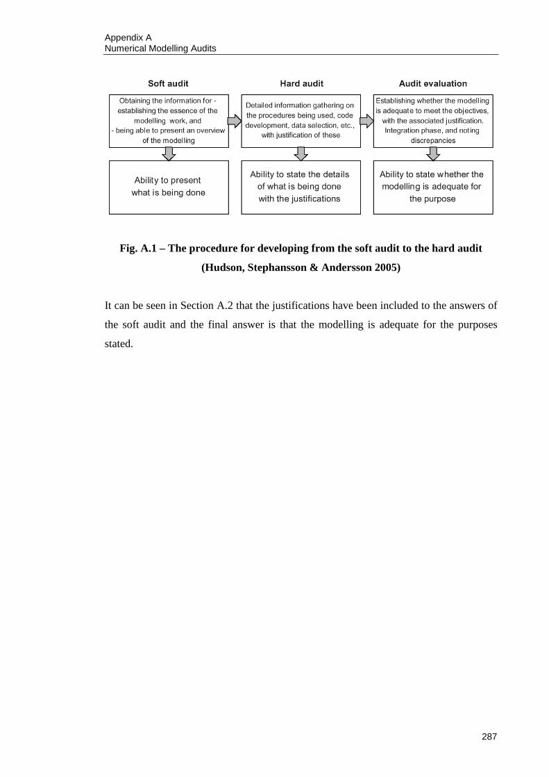
Appendix A Numerical Modelling Audits
287
Fig. A.1 – The procedure for developing from the soft audit to the hard audit
(Hudson, Stephansson & Andersson 2005)
It can be seen in Section A.2 that the justifications have been included to the answers of
the soft audit and the final answer is that the modelling is adequate for the purposes
stated.

Appendix B Single Longwall Panel Model With No River Valley
288
APPENDIX B SINGLE LONGWALL PANEL MODEL WITH NO
RIVER VALLEY
; Model based on Metropolitan Colliery
; Using symmetry
; Depth of cover = 413 m
; Longwall width = 105 m
; Extracted thickness = 2.7 m
; W/h ratio = 0.25
; Model dimensions: 815 m x 509.8 m
ti
Model 1 (Metropolitan Colliery)
; Creating model geometry
ro = 0.01
se ov = 0.2
bl 0,-509.8 0,0 815,0 815,-509.8
cr 0,-88 815,-88 ; Hawkesbury Sandstone (88 m thick)
cr 0,-108 815,-108 ; Newport Formation (20 m thick)
cr 0,-142 815,-142 ; Bald Hill Claystone (34 m thick)
cr 0,-287 815,-287 ; Bulgo Sandstone (145 m thick)
cr 0,-327 815,-327 ; Stanwell Park Claystone (40 m thick)
cr 0,-377 815,-377 ; Scarborough Sandstone (50 m thick)
cr 0,-393 815,-393 ; Wombarra Shale (16 m thick)
cr 0,-413 815,-413 ; Coal Cliff Sandstone (20 m thick)
cr 0,-415.7 815,-415.7 ; Bulli Seam (2.7 m thick)
cr 0,-423.7 815,-423.7 ; Loddon Sandstone (8 m thick)
cr 0,-424.7 815,-424.7 ; Balgownie Seam (1 m thick)
cr 0,-428.7 815,-428.7 ; Lawrence Sandstone (4 m thick)
cr 0,-430.7 815,-430.7 ; Cape Horn Seam (2 m thick)
cr 0,-436.7 815,-436.7 ; UN2 (6 m thick)
cr 0,-436.8 815,-436.8 ; Hargraves Coal Member (0.1 m thick)
cr 0,-446.8 815,-446.8 ; UN3 (10 m thick)
cr 0,-456.8 815,-456.8 ; Wongawilli Seam (10 m thick)
Appendix B Single Longwall Panel Model With No River Valley
289
cr 0,-459.8 815,-459.8 ; Kembla Sandstone (3 m thick)
cr 0,-509.8 815,-509.8 ; Coal Measures (50 m thick)
; Defining longwall
cr 762.5,-413 762.5,-415.7
cr 815,-413 815,-415.7
; Defining discontinuities
jr 0,-88 0,0 815,0 815,-88 ; Hawkesbury Sandstone
js 0,0 815,0 0,0 9,0
js 90,0 9,0 9,0 9,0
js 90,0 9,0 9,0 9,0 4.5 -9
jr 0,-108 0,-88 815,-88 815,-108 ; Newport Formation
js 0,0 815,0 0,0 1,0
js 90,0 1,0 1,0 1,0
js 90,0 1,0 1,0 1,0 0.5,-89
jr 0,-142 0,-108 815,-108 815,-142 ; Bald Hill Claystone
js 0,0 815,0 0,0 1,0
js 90,0 1,0 1,0 1,0
js 90,0 1,0 1,0 1,0 0.5,-109
jr 0,-287 0,-142 815,-142 815,-287 ; Bulgo Sandstone
js 0,0 815,0 0,0 9,0
js 90,0 9,0 9,0 9,0
js 90,0 9,0 9,0 9,0 4.5,-153
jr 0,-327 0,-287 815,-287 815,-327 ; Stanwell Park Claystone
js 0,0 815,0 0,0 3,0
js 90,0 3,0 3,0 3,0
js 90,0 3,0 3,0 3,0 1.5,-291
jr 0,-377 0,-327 815,-327 815,-377 ; Scarborough Sandstone
js 0,0 815,0 0,0 4,0
js 90,0 4,0 4,0 4,0
js 90,0 4,0 4,0 4,0 2,-332

Appendix B Single Longwall Panel Model With No River Valley
290
jr 0,-393 0,-377 815,-377 815,-393 ; Wombarra Shale
js 0,0 815,0 0,0 3,0
js 90,0 3,0 3,0 3,0
js 90,0 3,0 3,0 3,0 1.5,-381
jr 0,-413 0,-393 815,-393 815,-413 ; Coal Cliff Sandstone
js 0,0 815,0 0,0 3,0
js 90,0 3,0 3,0 3,0
js 90,0 3,0 3,0 3,0 1.5,-399
; Generating zones for deformable blocks
ge q 12.7 ra 0 815 -88 0 ; Hawkesbury Sandstone
ge q 1.4 ra 0 815 -108 -88 ; Newport Formation
ge q 1.4 ra 0 815 -142 -108 ; Bald Hill Claystone
ge q 12.7 ra 0 815 -287 -142 ; Bulgo Sandstone
ge q 4.2 ra 0 815 -327 -287 ; Stanwell Park Claystone
ge q 5.7 ra 0 815 -377 -327 ; Scarborough Sandstone
ge q 4.2 ra 0 815 -393 -377 ; Wombarra Shale
ge q 4.2 ra 0 815 -413 -393 ; Coal Cliff Sandstone
ge q 3.5 ra 0 815 -415.7 -413 ; Bulli Seam
ge q 11.3 ra 0 815 -423.7 -415.7 ; Loddon Sandstone
ge q 1.4 ra 0 815 -424.7 -423.7 ; Balgownie Seam
ge q 5.7 ra 0 815 -428.7 -424.7 ; Lawrence Sandstone
ge q 2.8 ra 0 815 -430.7 -428.7 ; Cape Horn Seam
ge q 8.5 ra 0 815 -436.7 -430.7 ; UN2
ge q 0.1 ra 0 815 -436.8 -436.7 ; Hargraves Coal Member
ge q 14.1 ra 0 815 -446.8 -436.8 ; UN3
ge q 14.1 ra 0 815 -456.8 -446.8 ; Wongawilli Seam
ge q 4.2 ra 0 815 -459.8 -456.8 ; Kembla Sandstone
ge q 4.2 ra 0 815 -509.8 -459.8 ; Coal Measures
sa model1_ini1.sav
; Defining material properties
pro m 1 de = 2397 b = 11.47e9 sh = 5.65e9 coh = 9.70e6 fr = 37.25 &
ten = 3.58e6 ; Hawkesbury Sandstone
pro m 2 de = 2290 b = 7.77e9 sh = 4.66e9 coh = 8.85e6 fr = 35.00 &
ten = 3.40e6 ; Newport Formation

Appendix B Single Longwall Panel Model With No River Valley
291
pro m 3 de = 2719 b = 14.12e9 sh = 4.72e9 coh = 10.60e6 fr = 27.80 &
ten = 2.90e6 ; Bald Hill Claystone
pro m 4 de = 2527 b = 12.60e9 sh = 7.91e9 coh = 17.72e6 fr = 35.40 &
ten = 6.55e6 ; Bulgo Sandstone
pro m 5 de = 2693 b = 13.22e9 sh = 7.63e9 coh = 14.57e6 fr = 27.80 &
ten =4 .83e6 ; Stanwell Park Claystone
pro m 6 de = 2514 b = 16.16e9 sh = 10.80e9 coh = 13.25e6 fr = 40.35 &
ten = 7.18e6 ; Scarborough Sandstone
pro m 7 de = 2643 b = 24.81e9 sh = 7.24e9 coh = 14.51e6 fr = 27.80 &
ten = 4.81e6 ; Wombarra Shale
pro m 8 de = 2600 b = 17.07e9 sh = 11.44e9 coh = 19.40e6 fr = 33.30 &
ten = 7.87e6 ; Coal Cliff Sandstone
pro m 9 de = 1500 b = 2.33e9 sh = 1.08e9 coh = 6.37e6 fr = 25.00 &
ten = 0.84e6 ; Bulli Seam
pro m 10 de = 2539 b = 16.76e9 sh = 6.51e9 coh = 17.10e6 fr = 28.90 &
ten = 5.65e6 ; Loddon Sandstone
pro m 11 de = 1500 b = 2.33e9 sh = 1.08e9 coh = 6.37e6 fr = 25.00 &
ten = 0.84e6 ; Balgownie Seam
pro m 12 de = 2539 b = 16.76e9 sh = 6.51e9 coh = 17.10e6 fr = 28.90 &
ten = 5.65e6 ; Lawrence Sandstone
pro m 13 de = 1500 b = 1.67e9 sh = 0.77e9 coh = 2.87e6 fr = 25.00 &
ten = 0.70e6 ; Cape Horn Seam
pro m 14 de = 2560 b = 8.99e9 sh = 5.39e9 coh = 19.89e6 fr = 28.90 &
ten = 6.74e6 ; UN2
pro m 15 de = 1500 b = 2.33e9 sh = 1.08e9 coh = 6.37e6 fr = 25.00 &
ten = 0.84e6 ; Hargraves Coal Member
pro m 16 de = 2620 b = 8.67e9 sh = 5.20e9 coh = 19.18e6 fr = 28.90 &
ten = 6.50e6 ; UN3

Appendix B Single Longwall Panel Model With No River Valley
292
pro m 17 de = 1500 b = 1.67e9 sh = 0.77e9 coh = 2.87e6 fr = 25.00 &
ten =0 .70e6 ; Wongawilli Seam
pro m 18 de = 2569 b = 13.79e9 sh = 7.12e9 coh = 18.02e6 fr = 28.90 &
ten = 6.11e6 ; Kembla Sandstone
pro m 19 de = 2092 b = 8.11e9 sh = 3.83e9 coh = 12.20e6 fr = 27.17 &
ten = 3.75e6 ; Coal Measures
; Assigning material properties
ch cons 3
ch m 1 ra 0 815 -88 0 ; Hawkesbury Sandstone
ch m 2 ra 0 815 -108 -88 ; Newport Formation
ch m 3 ra 0 815 -142 -108 ; Bald Hill Claystone
ch m 4 ra 0 815 -287 -142 ; Bulgo Sandstone
ch m 5 ra 0 815 -327 -287 ; Stanwell Park Claystone
ch m 6 ra 0 815 -377 -327 ; Scarborough Sandstone
ch m 7 ra 0 815 -393 -377 ; Wombarra Shale
ch m 8 ra 0 815 -413 -393 ; Coal Cliff Sandstone
ch m 9 ra 0 815 -415.7 -413 ; Bulli Seam
ch m 10 ra 0 815 -423.7 -415.7 ; Loddon Sandstone
ch m 11 ra 0 815 -424.7 -423.7 ; Balgownie Seam
ch m 12 ra 0 815 -428.7 -424.7 ; Lawrence Sandstone
ch m 13 ra 0 815 -430.7 -428.7 ; Cape Horn Seam
ch m 14 ra 0 815 -436.7 -430.7 ; UN2
ch m 15 ra 0 815 -436.8 -436.7 ; Hargraves Coal Member
ch m 16 ra 0 815 -446.8 -436.8 ; UN3
ch m 17 ra 0 815 -456.8 -446.8 ; Wongawilli Seam
ch m 18 ra 0 815 -459.8 -456.8 ; Kembla Sandstone
ch m 19 ra 0 815 -509.8 -459.8 ; Coal Measures
; Defining bedding plane properties
pro jm = 1 jkn = 21e9 jks = 2.1e9 & ; Hawkesbury Sandstone
jf = 25 jrf = 15 &
jc = 0.29e6 jresc = 0

Appendix B Single Longwall Panel Model With No River Valley
293
pro jm = 2 jkn = 140e9 jks = 14e9 & ; Newport Formation
jf = 25 jrf = 15 &
jc = 0.29e6 jresc = 0
pro jm = 3 jkn = 204e9 jks = 20.4e9 & ; Bald Hill Claystone
jf = 25 jrf = 15 &
jc = 0.29e6 jresc = 0
pro jm = 4 jkn = 26e9 jks = 2.6e9 & ; Bulgo Sandstone
jf = 25 jrf = 15 &
jc = 0.29e6 jresc = 0
pro jm = 5 jkn = 78e9 jks = 7.8e9 & ; Stanwell Park Claystone
jfc = 25 jrf = 15 &
jc = 0.29e6 jresc = 0
pro jm = 6 jkn = 76e9 jks = 7.6e9 & ; Scarborough Sandstone
jf = 25 jrf = 15 &
jc = 0.29e6 jresc = 0
pro jm = 7 jkn = 115e9 jks = 11.5e9 & ; Wombarra Shale
jf = 25 jrf = 15 &
jc = 0.29e6 jresc = 0
pro jm = 8 jkn = 400e9 jks = 40e9 & ; Coal Cliff Sandstone
jf = 25 jrf = 15 &
jc = 0.29e6 jresc = 0
pro jm = 9 jkn = 400e9 jks = 40e9 & ; Sub Bulli
jf = 25 jrf = 15 &
jc = 0.29e6 jresc = 0
; Assigning bedding plane properties
ch jc = 5 ra 0 815 -509.8 0 ang -1 1
se jc = 5
ch jm 1 ra 0 815 -88 0 ang -1 1 ; Hawkesbury Sandstone
ch jm 2 ra 0 815 -108 -88 ang -1 1 ; Newport Formation
ch jm 3 ra 0 815 -142 -108 ang -1 1 ; Bald Hill Claystone
ch jm 4 ra 0 815 -287 -142 ang -1 1 ; Bulgo Sandstone

Appendix B Single Longwall Panel Model With No River Valley
294
ch jm 5 ra 0 815 -327 -287 ang -1 1 ; Stanwell Park Claystone
ch jm 6 ra 0 815 -377 -327 ang -1 1 ; Scarborough Sandstone
ch jm 7 ra 0 815 -393 -377 ang -1 1 ; Wombarra Shale
ch jm 8 ra 0 815 -413 -393 ang -1 1 ; Coal Cliff Sandstone
ch jm 9 ra 0 815 -509.8 -413 ang -1 1 ; Sub Bulli
; Defining vertical joint properties
pro jm = 10 jkn = 21e9 jks = 2.1e9 & ; Hawkesbury Sandstone
jf = 19 jrf = 15 &
jc = 0.86e6 jresc = 0
pro jm = 11 jkn = 140e9 jks = 14e9 & ; Newport Formation
jf = 19 jrf = 15 &
jc = 0.86e6 jresc = 0
pro jm = 12 jkn = 204e9 jks = 20.4e9 & ; Bald Hill Claystone
jf = 19 jrf = 15 &
jc = 0.86e6 jresc = 0
pro jm = 13 jkn = 26e9 jks = 2.6e9 & ; Bulgo Sandstone
jf = 19 jrf = 15 &
jc = 0.86e6 jresc = 0
pro jm = 14 jkn = 78e9 jks = 7.8e9 & ; Stanwell Park Claystone
jf = 19 jrf = 15 &
jc = 0.86e6 jresc = 0
pro jm = 15 jkn = 76e9 jks = 7.6e9 & ; Scarborough Sandstone
jf = 19 jrf = 15 &
jc = 0.86e6 jresc = 0
pro jm = 16 jkn = 115e9 jks = 11.5e9 & ; Wombarra Shale
jf = 19 jrf = 15 &
jc = 0.86e6 jresc = 0
pro jm = 17 jkn = 400e9 jks = 40e9 & ; Coal Cliff Sandstone
jf = 19 jrf = 15 &
jc = 0.86e6 jresc = 0
Appendix B Single Longwall Panel Model With No River Valley
295
pro jm = 18 jkn = 400e9 jks = 40e9 & ; Sub Bulli
jf = 19 jrf = 15 &
jc = 0.86e6 jresc = 0
; Assigning vertical joint properties
ch jc = 5 ra 0 815 -509.8 0 ang 89 91
se jc = 5
ch jm 10 ra 0 815 -88 0 ang 89 91 ; Hawkesbury Sandstone
ch jm 11 ra 0 815 -108 -88 ang 89 91 ; Newport Formation
ch jm 12 ra 0 815 -142 -108 ang 89 91 ; Bald Hill Claystone
ch jm 13 ra 0 815 -287 -142 ang 89 91 ; Bulgo Sandstone
ch jm 14 ra 0 815 -327 -287 ang 89 91 ; Stanwell Park Claystone
ch jm 15 ra 0 815 -377 -327 ang 89 91 ; Scarborough Sandstone
ch jm 16 ra 0 815 -393 -377 ang 89 91 ; Wombarra Shale
ch jm 17 ra 0 815 -413 -393 ang 89 91 ; Coal Cliff Sandstone
ch jm 18 ra 0 815 -509.8 -413 ang 89 91 ; Sub Bulli
; Defining gravity
se gr 0 -9.81
; Defining boundary conditions
bo xv 0 ra -0.1 0.1 -509.8 0
bo xv 0 ra 814.9 815.1 -509.8,0
bo yv 0 ra 0 815 -509.9 -509.7
; Defining initial stress conditions
in st 0 0 0 yg 4.82e4 0 2.41e4 szz 0 zg 0 4.82e4 ra 0 815 -509.8 0
da a
so
sa model1_ini2.sav
Appendix B Single Longwall Panel Model With No River Valley
296
; Initialising displacements
rese vel
rese di
; Defining histories
; Y-displacements
hi yd 0 0 ;1
hi yd 4.5 0 ;2
hi yd 13.5 0 ;3
hi yd 22.5 0 ;4
hi yd 31.5 0 ;5
hi yd 40.5 0 ;6
hi yd 49.5 0 ;7
hi yd 58.5 0 ;8
hi yd 67.5 0 ;9
hi yd 76.5 0 ;10
hi yd 85.5 0 ;11
hi yd 94.5 0 ;12
hi yd 103.5 0 ;13
hi yd 112.5 0 ;14
hi yd 121.5 0 ;15
hi yd 130.5 0 ;16
hi yd 139.5 0 ;17
hi yd 148.5 0 ;18
hi yd 157.5 0 ;19
hi yd 166.5 0 ;20
hi yd 175.5 0 ;21
hi yd 184.5 0 ;22
hi yd 193.5 0 ;23
hi yd 202.5 0 ;24
hi yd 211.5 0 ;25
hi yd 220.5 0 ;26
hi yd 229.5 0 ;27
hi yd 238.5 0 ;28
hi yd 247.5 0 ;29
hi yd 256.5 0 ;30
hi yd 265.5 0 ;31
hi yd 274.5 0 ;32
hi yd 283.5 0 ;33

Appendix B Single Longwall Panel Model With No River Valley
297
hi yd 292.5 0 ;34
hi yd 301.5 0 ;35
hi yd 310.5 0 ;36
hi yd 319.5 0 ;37
hi yd 328.5 0 ;38
hi yd 337.5 0 ;39
hi yd 346.5 0 ;40
hi yd 355.5 0 ;41
hi yd 364.5 0 ;42
hi yd 373.5 0 ;43
hi yd 382.5 0 ;44
hi yd 391.5 0 ;45
hi yd 400.5 0 ;46
hi yd 409.5 0 ;47
hi yd 418.5 0 ;48
hi yd 427.5 0 ;49
hi yd 436.5 0 ;50
hi yd 445.5 0 ;51
hi yd 454.5 0 ;52
hi yd 463.5 0 ;53
hi yd 472.5 0 ;54
hi yd 481.5 0 ;55
hi yd 490.5 0 ;56
hi yd 499.5 0 ;57
hi yd 508.5 0 ;58
hi yd 517.5 0 ;59
hi yd 526.5 0 ;60
hi yd 535.5 0 ;61
hi yd 544.5 0 ;62
hi yd 553.5 0 ;63
hi yd 562.5 0 ;64
hi yd 571.5 0 ;65
hi yd 580.5 0 ;66
hi yd 589.5 0 ;67
hi yd 598.5 0 ;68
hi yd 607.5 0 ;69
hi yd 616.5 0 ;70
hi yd 625.5 0 ;71
hi yd 634.5 0 ;72
hi yd 643.5 0 ;73
hi yd 652.5 0 ;74

Appendix B Single Longwall Panel Model With No River Valley
298
hi yd 661.5 0 ;75
hi yd 670.5 0 ;76
hi yd 679.5 0 ;77
hi yd 688.5 0 ;78
hi yd 697.5 0 ;79
hi yd 706.5 0 ;80
hi yd 715.5 0 ;81
hi yd 724.5 0 ;82
hi yd 733.5 0 ;83
hi yd 742.5 0 ;84
hi yd 751.5 0 ;85
hi yd 760.5 0 ;86
hi yd 769.5 0 ;87
hi yd 778.5 0 ;88
hi yd 787.5 0 ;89
hi yd 796.5 0 ;90
hi yd 805.5 0 ;91
hi yd 814.5 0 ;92
hi yd 815.0 0 ;93
; X-displacements
hi xd 0 0 ;94
hi xd 4.5 0 ;95
hi xd 13.5 0 ;96
hi xd 22.5 0 ;97
hi xd 31.5 0 ;98
hi xd 40.5 0 ;99
hi xd 49.5 0 ;100
hi xd 58.5 0 ;101
hi xd 67.5 0 ;102
hi xd 76.5 0 ;103
hi xd 85.5 0 ;104
hi xd 94.5 0 ;105
hi xd 103.5 0 ;106
hi xd 112.5 0 ;107
hi xd 121.5 0 ;108
hi xd 130.5 0 ;109
hi xd 139.5 0 ;110
hi xd 148.5 0 ;111
hi xd 157.5 0 ;112

Appendix B Single Longwall Panel Model With No River Valley
299
hi xd 166.5 0 ;113
hi xd 175.5 0 ;114
hi xd 184.5 0 ;115
hi xd 193.5 0 ;116
hi xd 202.5 0 ;117
hi xd 211.5 0 ;118
hi xd 220.5 0 ;119
hi xd 229.5 0 ;120
hi xd 238.5 0 ;121
hi xd 247.5 0 ;122
hi xd 256.5 0 ;123
hi xd 265.5 0 ;124
hi xd 274.5 0 ;125
hi xd 283.5 0 ;126
hi xd 292.5 0 ;127
hi xd 301.5 0 ;128
hi xd 310.5 0 ;129
hi xd 319.5 0 ;130
hi xd 328.5 0 ;131
hi xd 337.5 0 ;132
hi xd 346.5 0 ;133
hi xd 355.5 0 ;134
hi xd 364.5 0 ;135
hi xd 373.5 0 ;136
hi xd 382.5 0 ;137
hi xd 391.5 0 ;138
hi xd 400.5 0 ;139
hi xd 409.5 0 ;140
hi xd 418.5 0 ;141
hi xd 427.5 0 ;142
hi xd 436.5 0 ;143
hi xd 445.5 0 ;144
hi xd 454.5 0 ;145
hi xd 463.5 0 ;146
hi xd 472.5 0 ;147
hi xd 481.5 0 ;148
hi xd 490.5 0 ;149
hi xd 499.5 0 ;150
hi xd 508.5 0 ;151
hi xd 517.5 0 ;152
hi xd 526.5 0 ;153

Appendix B Single Longwall Panel Model With No River Valley
300
hi xd 535.5 0 ;154
hi xd 544.5 0 ;155
hi xd 553.5 0 ;156
hi xd 562.5 0 ;157
hi xd 571.5 0 ;158
hi xd 580.5 0 ;159
hi xd 589.5 0 ;160
hi xd 598.5 0 ;161
hi xd 607.5 0 ;162
hi xd 616.5 0 ;163
hi xd 625.5 0 ;164
hi xd 634.5 0 ;165
hi xd 643.5 0 ;166
hi xd 652.5 0 ;167
hi xd 661.5 0 ;168
hi xd 670.5 0 ;169
hi xd 679.5 0 ;170
hi xd 688.5 0 ;171
hi xd 697.5 0 ;172
hi xd 706.5 0 ;173
hi xd 715.5 0 ;174
hi xd 724.5 0 ;175
hi xd 733.5 0 ;176
hi xd 742.5 0 ;177
hi xd 751.5 0 ;178
hi xd 760.5 0 ;179
hi xd 769.5 0 ;180
hi xd 778.5 0 ;181
hi xd 787.5 0 ;182
hi xd 796.5 0 ;183
hi xd 805.5 0 ;184
hi xd 814.5 0 ;185
hi xd 815.0 0 ;186
hi u ;187
; Extracting longwall - instantaneous extraction
de b 4098
da a

Appendix B Single Longwall Panel Model With No River Valley
301
; Solving for equilibrium
so rat 1e-5 ste 1000000000
sa model1_final.sav
Appendix C River Valley Model With Plane At Base
302
APPENDIX C RIVER VALLEY MODEL WITH PLANE AT BASE
ti
Valley 1
; Creating model geometry
ro = 0.01
set ov = 0.2
bl 0,-189 0,0 1050,0 1050,-189
cr 0,-78 1050,-78 ; Hawkesbury Sandstone (78 m thick)
cr 0,-85 1050,-85 ; Newport Formation (7 m thick)
cr 0,-97 1050,-97 ; Bald Hill Claystone (9 m thick)
cr 0,-186 1050,-186 ; Bulgo Sandstone (89 m thick + 3 m thick beam)
; Generating vertical cracks for beam at base of Bald Hill Claystone
jr 0,-189 0,-186 525,-186 525,-189
js 90,0 3,0 0,0 9,0 13.5,-189
cr 525,-189 525,-186
cr 532.5,-189 532.5,-186
jr 532.5,-189 532.5,-186 1050,-186 1050,-189
js 90,0 3,0 0,0 9,0 1045.5,-189
; Generating pre-defined cracks for valleys (70 m deep x 50 m wide)
cr 0,-70 1050,-70
cr 500,-70 500,0
cr 450,-70 450,0
cr 400,-70 400,0
cr 350,-70 350,0
cr 300,-70 300,0
cr 250,-70 250,0
cr 200,-70 200,0
cr 150,-70 150,0
cr 100,-70 100,0

Appendix C River Valley Model With Plane At Base
303
cr 50,-70 50,0
cr 550,-70 550,0
cr 600,-70 600,0
cr 650,-70 650,0
cr 700,-70 700,0
cr 750,-70 750,0
cr 800,-70 800,0
cr 850,-70 850,0
cr 900,-70 900,0
cr 950,-70 950,0
cr 1000,-70 1000,0
; Defining discontinuities
jr 0,-78 0,-70 1050,-70 1050,-78 ; Hawkesbury Sandstone
js 90,0 9,0 9,0 9,0 4.5 -78
jr 0,-85 0,-78 1050,-78 1050,-85 ; Newport Formation
js 0,0 1050,0 0,0 1,0
js 90,0 1,0 1,0 1,0
js 90,0 1,0 1,0 1,0 0.5,-79
jr 0,-97 0,-85 1050,-85 1050,-97 ; Bald Hill Claystone
js 0,0 1050,0 0,0 1,0
js 90,0 1,0 1,0 1,0
js 90,0 1,0 1,0 1,0 0.5,-87
jr 0,-186 0,-97 1050,-97 1050,-186 ; Bulgo Sandstone
js 0,0 525,0 0,0 9,0
js 90,0 9,0 9,0 9,0
js 90,0 9,0 9,0 9,0 4.5,-117
jr 0,-189 0,-186 525,-186 525,-189
js 90,0 3,0 0,0 9,0 13.5,-189
cr 525,-189 525,-186
cr 532.5,-189 532.5,-186
jr 532.5,-189 532.5,-186 1050,-186 1050,-189
js 90,0 3,0 0,0 9,0 1045.5,-189

Appendix C River Valley Model With Plane At Base
304
; Generating zones for deformable blocks
ge q 12.7 ra 0 1050 -78 0 ; Hawkesbury Sandstone
ge q 1.4 ra 0 1050 -85 -78 ; Newport Formation
ge q 1.4 ra 0 1050 -97 -85 ; Bald Hill Claystone
ge q 12.7 ra 0 1050 -189 -97 ; Bulgo Sandstone
; Defining material properties
pro m 1 de = 2397 b = 11.47e9 sh = 5.65e9 coh = 9.70e6 fr= 37.25 &
ten = 3.58e6 ; Hawkesbury Sandstone
pro m 2 de = 2290 b = 7.77e9 sh = 4.66e9 coh = 8.85e6 fr= 35.00 &
ten = 3.40e6 ; Newport Formation
pro m 3 de = 2719 b = 14.12e9 sh = 4.72e9 coh = 10.60e6 fr= 27.80 &
ten = 2.90e6 ; Bald Hill Claystone
pro m 4 de = 2527 b = 12.60e9 sh = 7.91e9 coh = 17.72e6 fr= 35.40 &
ten = 6.55e6 ; Bulgo Sandstone
; Assigning material properties
ch cons 3
ch m 1 ra 0 1050 -78 0 ; Hawkesbury Sandstone
ch m 2 ra 0 1050 -85 -78 ; Newport Formation
ch m 3 ra 0 1050 -97 -85 ; Bald Hill Claystone
ch m 4 ra 0 1050 -189 -97 ; Bulgo Sandstone
; Defining bedding plane properties
pro jm = 1 jkn = 21e9 jks = 2.1e9 & ; Hawkesbury Sandstone
jf = 25 jrf = 15 &
jc = 0.29e6 jresc = 0
pro jm = 2 jkn = 140e9 jks = 14.0e9 & ; Newport Formation
jf = 25 jrf = 15 &
jc = 0.29e6 jresc = 0

Appendix C River Valley Model With Plane At Base
305
pro jm = 3 jkn = 204e9 jks = 20.4e9 & ; Bald Hill Claystone
jf = 25 jrf = 15 &
jc = 0.29e6 jresc = 0
pro jm = 4 jkn = 26e9 jks = 2.6e9 & ; Bulgo Sandstone
jf = 25 jrf = 15 &
jc = 0.29e6 jresc = 0
pro jm = 5 jkn = 204e9 jks = 20.4e9 & ; Beam
jf = 89 jrf = 89 &
jc = 1e10 jresc = 1e10 &
jt = 1e10 jrt = 1e10
; Assigning bedding plane properties
ch jc = 5 ra 0 1050 -189 0 ang -1 1
se jc = 5
ch jm 1 ra 0 1050 -78 0 ang -1 1 ; Hawkesbury Sandstone
ch jm 2 ra 0 1050 -85 -78 ang -1 1 ; Newport Formation
ch jm 3 ra 0 1050 -97 -85 ang -1 1 ; Bald Hill Claystone
ch jm 4 ra 0 1050 -186 -97 ang -1 1 ; Bulgo Sandstone
ch jm 5 ra 0 1050 -189 -186 ang -1 1 ; Beam
; Vertical joint properties
pro jm = 6 jkn = 21e9 jks = 2.1e9 & ; Hawkesbury Sandstone
jf = 19 jrf = 15 &
jc = 0.86e6 jresc = 0
pro jm = 7 jkn = 140e9 jks = 14.0e9 & ; Newport Formation
jf = 19 jrf = 15 &
jc = 0.86e6 jresc = 0
pro jm = 8 jkn = 204e9 jks = 20.4e9 & ; Bald Hill Claystone
jf = 19 jrf = 15 &
jc = 0.86e6 jresc = 0
pro jm = 9 jkn = 26e9 jks = 2.6e9 & ; Bulgo Sandstone;
jf = 19 jrf = 15 &
jc = 0.86e6 jresc = 0

Appendix C River Valley Model With Plane At Base
306
pro jm = 10 jkn = 204e9 jks = 20.4e9 & ; Beam
jf = 89 jrf = 89 &
jc = 1e10 jresc = 1e10 &
jt = 1e10 jrt = 1e10
; Assigning vertical joint properties
ch jc = 5 ra 0 1050 -189 0 ang 89 91
se jc = 5
ch jm 6 ra 0 1050 -186 0 ang 89 91 ; Hawkesbury Sandstone
ch jm 7 ra 0 1050 -85 -78 ang 89 91 ; Newport Formation
ch jm 8 ra 0 1050 -97 -85 ang 89 91 ; Bald Hill Claystone
ch jm 9 ra 0 1050 -186 -97 ang 89 91 ; Bulgo Sandstone
ch jm 10 ra 0 1050 -189 -186 ang 89 91 ; Beam
; Defining gravity
se gr 0 -9.81
; Defining boundary conditions
bo yv 0 ra 0 1050 -189.1 -188.9
bo xv 0 ra -0.1 0.1 -189.1 0.1
bo xv 0 ra 1049.9 1050.1 -189.1 0.1
; Defining initial stress conditions
in st 0 0 0 yg 4.77e4 0 2.39e4 szz 0 zg 0 4.77e4 ra 0 1050 -189 0
sa valley1_ini1.sav
; Cycle to equilibrium
da a
so

Appendix C River Valley Model With Plane At Base
307
; Removing valley and cycle to equilibrium
de ra 500 550 -70 0
da a
so
; Removing boundary conditions at base and attaching pre-determined y-
displacements
rese vel
rese di
bo yfr
bo xfr
bo xv 0 ra -0.1 0.1 -189.1 0.1
bo xv 0 ra 1049.9 1050.1 -189.1 0.1
; Histories
; X Displacements (valley closure)
; Top of valley
hi xd 50 0 ;1
hi xd 100 0 ;2
hi xd 150 0 ;3
hi xd 200 0 ;4
hi xd 250 0 ;5
hi xd 300 0 ;6
hi xd 350 0 ;7
hi xd 400 0 ;8
hi xd 450 0 ;9
hi xd 500 0 ;10
hi xd 550 0 ;11
; Y Displacements (subsidence)
hi yd 0 0 ;12
hi yd 25 0 ;13
hi yd 50 0 ;14

Appendix C River Valley Model With Plane At Base
308
hi yd 75 0 ;15
hi yd 100 0 ;16
hi yd 125 0 ;17
hi yd 150 0 ;18
hi yd 175 0 ;19
hi yd 200 0 ;20
hi yd 225 0 ;21
hi yd 250 0 ;22
hi yd 275 0 ;23
hi yd 300 0 ;24
hi yd 325 0 ;25
hi yd 350 0 ;26
hi yd 375 0 ;27
hi yd 400 0 ;28
hi yd 425 0 ;29
hi yd 450 0 ;30
hi yd 475 0 ;31
hi yd 500 0 ;32
hi yd 525 0 ;33
hi yd 550 0 ;34
hi yd 575 0 ;35
hi yd 600 0 ;36
hi yd 625 0 ;37
hi yd 650 0 ;38
hi yd 675 0 ;39
hi yd 700 0 ;40
hi yd 725 0 ;41
hi yd 750 0 ;42
hi yd 775 0 ;43
hi yd 800 0 ;44
hi yd 825 0 ;45
hi yd 850 0 ;46
hi yd 875 0 ;47
hi yd 900 0 ;48
hi yd 925 0 ;49
hi yd 950 0 ;50
hi yd 975 0 ;51
hi yd 1000 0 ;52
hi yd 1025 0 ;53
hi yd 1050 0 ;54
Appendix C River Valley Model With Plane At Base
309
; Y displacements (base)
hi yd 0 -189 ;55
hi yd 4.5 -189 ;56
hi yd 13.5 -189 ;57
hi yd 22.5 -189 ;58
hi yd 31.5 -189 ;59
hi yd 40.5 -189 ;60
hi yd 49.5 -189 ;61
hi yd 58.5 -189 ;62
hi yd 67.5 -189 ;63
hi yd 76.5 -189 ;64
hi yd 85.5 -189 ;65
hi yd 94.5 -189 ;66
hi yd 103.5 -189 ;67
hi yd 112.5 -189 ;68
hi yd 121.5 -189 ;69
hi yd 130.5 -189 ;70
hi yd 139.5 -189 ;71
hi yd 148.5 -189 ;72
hi yd 157.5 -189 ;73
hi yd 166.5 -189 ;74
hi yd 175.5 -189 ;75
hi yd 184.5 -189 ;76
hi yd 193.5 -189 ;77
hi yd 202.5 -189 ;78
hi yd 211.5 -189 ;79
hi yd 220.5 -189 ;80
hi yd 229.5 -189 ;81
hi yd 238.5 -189 ;82
hi yd 247.5 -189 ;83
hi yd 256.5 -189 ;84
hi yd 265.5 -189 ;85
hi yd 274.5 -189 ;86
hi yd 283.5 -189 ;87
hi yd 292.5 -189 ;88
hi yd 301.5 -189 ;89
hi yd 310.5 -189 ;90
hi yd 319.5 -189 ;91
hi yd 328.5 -189 ;92
hi yd 337.5 -189 ;93

Appendix C River Valley Model With Plane At Base
310
hi yd 346.5 -189 ;94
hi yd 355.5 -189 ;95
hi yd 364.5 -189 ;96
hi yd 373.5 -189 ;97
hi yd 382.5 -189 ;98
hi yd 391.5 -189 ;99
hi yd 400.5 -189 ;100
hi yd 409.5 -189 ;101
hi yd 418.5 -189 ;102
hi yd 427.5 -189 ;103
hi yd 436.5 -189 ;104
hi yd 445.5 -189 ;105
hi yd 454.5 -189 ;106
hi yd 463.5 -189 ;107
hi yd 472.5 -189 ;108
hi yd 481.5 -189 ;109
hi yd 490.5 -189 ;110
hi yd 499.5 -189 ;111
hi yd 508.5 -189 ;112
hi yd 517.5 -189 ;113
hi yd 525.0 -189 ;114
; Creating y-velocities at base and final solving routine
def valleysolve
; Step 1 to obtain time step
command
cyc 1
end_command
; Identifying gridpoints at base to which velocities will be attached
gri_chk1 = gp_near(0.0,-189)
gri_chk2 = gp_near(4.5,-189)
gri_chk3 = gp_near(13.5,-189)
gri_chk4 = gp_near(22.5,-189)
gri_chk5 = gp_near(31.5,-189)
gri_chk6 = gp_near(40.5,-189)
gri_chk7 = gp_near(49.5,-189)

Appendix C River Valley Model With Plane At Base
311
gri_chk8 = gp_near(58.5,-189)
gri_chk9 = gp_near(67.5,-189)
gri_chk10 = gp_near(76.5,-189)
gri_chk11 = gp_near(85.5,-189)
gri_chk12 = gp_near(94.5,-189)
gri_chk13 = gp_near(103.5,-189)
gri_chk14 = gp_near(112.5,-189)
gri_chk15 = gp_near(121.5,-189)
gri_chk16 = gp_near(130.5,-189)
gri_chk17 = gp_near(139.5,-189)
gri_chk18 = gp_near(148.5,-189)
gri_chk19 = gp_near(157.5,-189)
gri_chk20 = gp_near(166.5,-189)
gri_chk21 = gp_near(175.5,-189)
gri_chk22 = gp_near(184.5,-189)
gri_chk23 = gp_near(193.5,-189)
gri_chk24 = gp_near(202.5,-189)
gri_chk25 = gp_near(211.5,-189)
gri_chk26 = gp_near(220.5,-189)
gri_chk27 = gp_near(229.5,-189)
gri_chk28 = gp_near(238.5,-189)
gri_chk29 = gp_near(247.5,-189)
gri_chk30 = gp_near(256.5,-189)
gri_chk31 = gp_near(265.5,-189)
gri_chk32 = gp_near(274.5,-189)
gri_chk33 = gp_near(283.5,-189)
gri_chk34 = gp_near(292.5,-189)
gri_chk35 = gp_near(301.5,-189)
gri_chk36 = gp_near(310.5,-189)
gri_chk37 = gp_near(319.5,-189)
gri_chk38 = gp_near(328.5,-189)
gri_chk39 = gp_near(337.5,-189)
gri_chk40 = gp_near(346.5,-189)
gri_chk41 = gp_near(355.5,-189)
gri_chk42 = gp_near(364.5,-189)
gri_chk43 = gp_near(373.5,-189)
gri_chk44 = gp_near(382.5,-189)
gri_chk45 = gp_near(391.5,-189)
gri_chk46 = gp_near(400.5,-189)
gri_chk47 = gp_near(409.5,-189)
gri_chk48 = gp_near(418.5,-189)

Appendix C River Valley Model With Plane At Base
312
gri_chk49 = gp_near(427.5,-189)
gri_chk50 = gp_near(436.5,-189)
gri_chk51 = gp_near(445.5,-189)
gri_chk52 = gp_near(454.5,-189)
gri_chk53 = gp_near(463.5,-189)
gri_chk54 = gp_near(472.5,-189)
gri_chk55 = gp_near(481.5,-189)
gri_chk56 = gp_near(490.5,-189)
gri_chk57 = gp_near(499.5,-189)
gri_chk58 = gp_near(508.5,-189)
gri_chk59 = gp_near(517.5,-189)
gri_chk60 = gp_near(525.0,-189)
gri_chk61 = gp_near(532.5,-189)
gri_chk62 = gp_near(541.5,-189)
gri_chk63 = gp_near(550.5,-189)
gri_chk64 = gp_near(559.5,-189)
gri_chk65 = gp_near(568.5,-189)
gri_chk66 = gp_near(577.5,-189)
gri_chk67 = gp_near(586.5,-189)
gri_chk68 = gp_near(595.5,-189)
gri_chk69 = gp_near(604.5,-189)
gri_chk70 = gp_near(613.5,-189)
gri_chk71 = gp_near(622.5,-189)
gri_chk72 = gp_near(631.5,-189)
gri_chk73 = gp_near(640.5,-189)
gri_chk74 = gp_near(649.5,-189)
gri_chk75 = gp_near(658.5,-189)
gri_chk76 = gp_near(667.5,-189)
gri_chk77 = gp_near(676.5,-189)
gri_chk78 = gp_near(685.5,-189)
gri_chk79 = gp_near(694.5,-189)
gri_chk80 = gp_near(703.5,-189)
gri_chk81 = gp_near(712.5,-189)
gri_chk82 = gp_near(721.5,-189)
gri_chk83 = gp_near(730.5,-189)
gri_chk84 = gp_near(739.5,-189)
gri_chk85 = gp_near(748.5,-189)
gri_chk86 = gp_near(757.5,-189)
gri_chk87 = gp_near(766.5,-189)
gri_chk88 = gp_near(775.5,-189)
gri_chk89 = gp_near(784.5,-189)
Appendix C River Valley Model With Plane At Base
313
gri_chk90 = gp_near(793.5,-189)
gri_chk91 = gp_near(802.5,-189)
gri_chk92 = gp_near(811.5,-189)
gri_chk93 = gp_near(820.5,-189)
gri_chk94 = gp_near(829.5,-189)
gri_chk95 = gp_near(838.5,-189)
gri_chk96 = gp_near(847.5,-189)
gri_chk97 = gp_near(856.5,-189)
gri_chk98 = gp_near(865.5,-189)
gri_chk99 = gp_near(874.5,-189)
gri_chk100 = gp_near(883.5,-189)
gri_chk101 = gp_near(892.5,-189)
gri_chk102 = gp_near(901.5,-189)
gri_chk103 = gp_near(910.5,-189)
gri_chk104 = gp_near(919.5,-189)
gri_chk105 = gp_near(928.5,-189)
gri_chk106 = gp_near(937.5,-189)
gri_chk107 = gp_near(946.5,-189)
gri_chk108 = gp_near(955.5,-189)
gri_chk109 = gp_near(964.5,-189)
gri_chk110 = gp_near(973.5,-189)
gri_chk111 = gp_near(982.5,-189)
gri_chk112 = gp_near(991.5,-189)
gri_chk113 = gp_near(1000.5,-189)
gri_chk114 = gp_near(1009.5,-189)
gri_chk115 = gp_near(1018.5,-189)
gri_chk116 = gp_near(1027.5,-189)
gri_chk117 = gp_near(1036.5,-189)
gri_chk118 = gp_near(1045.5,-189)
gri_chk119 = gp_near(1050.0,-189)
; Defining y-displacements from Model 4
max_disp1 = 1.398e-03
max_disp2 = 1.394e-03
max_disp3 = 1.372e-03
max_disp4 = 1.331e-03
max_disp5 = 1.270e-03
max_disp6 = 1.188e-03
max_disp7 = 1.086e-03
max_disp8 = 9.621e-04
Appendix C River Valley Model With Plane At Base
314
max_disp9 = 8.172e-04
max_disp10 = 6.505e-04
max_disp11 = 4.614e-04
max_disp12 = 2.494e-04
max_disp13 = 1.411e-05
max_disp14 = -2.455e-04
max_disp15 = -5.299e-04
max_disp16 = -8.401e-04
max_disp17 = -1.177e-03
max_disp18 = -1.542e-03
max_disp19 = -1.937e-03
max_disp20 = -2.362e-03
max_disp21 = -2.820e-03
max_disp22 = -3.313e-03
max_disp23 = -3.843e-03
max_disp24 = -4.413e-03
max_disp25 = -5.027e-03
max_disp26 = -5.686e-03
max_disp27 = -6.396e-03
max_disp28 = -7.159e-03
max_disp29 = -7.980e-03
max_disp30 = -8.861e-03
max_disp31 = -9.804e-03
max_disp32 = -1.081e-02
max_disp33 = -1.190e-02
max_disp34 = -1.306e-02
max_disp35 = -1.430e-02
max_disp36 = -1.562e-02
max_disp37 = -1.703e-02
max_disp38 = -1.854e-02
max_disp39 = -2.014e-02
max_disp40 = -2.185e-02
max_disp41 = -2.367e-02
max_disp42 = -2.563e-02
max_disp43 = -2.778e-02
max_disp44 = -3.024e-02
max_disp45 = -3.344e-02
max_disp46 = -3.810e-02
max_disp47 = -4.513e-02
max_disp48 = -5.516e-02
max_disp49 = -6.945e-02

Appendix C River Valley Model With Plane At Base
315
max_disp50 = -9.050e-02
max_disp51 = -1.225e-01
max_disp52 = -1.700e-01
max_disp53 = -2.312e-01
max_disp54 = -2.952e-01
max_disp55 = -3.600e-01
max_disp56 = -4.214e-01
max_disp57 = -4.754e-01
max_disp58 = -5.190e-01
max_disp59 = -5.502e-01
max_disp60 = -2.362e+00
max_disp61 = -5.502e-01
max_disp62 = -5.190e-01
max_disp63 = -4.754e-01
max_disp64 = -4.214e-01
max_disp65 = -3.600e-01
max_disp66 = -2.952e-01
max_disp67 = -2.312e-01
max_disp68 = -1.700e-01
max_disp69 = -1.225e-01
max_disp70 = -9.050e-02
max_disp71 = -6.945e-02
max_disp72 = -5.516e-02
max_disp73 = -4.513e-02
max_disp74 = -3.810e-02
max_disp75 = -3.344e-02
max_disp76 = -3.024e-02
max_disp77 = -2.778e-02
max_disp78 = -2.563e-02
max_disp79 = -2.367e-02
max_disp80 = -2.185e-02
max_disp81 = -2.014e-02
max_disp82 = -1.854e-02
max_disp83 = -1.703e-02
max_disp84 = -1.562e-02
max_disp85 = -1.430e-02
max_disp86 = -1.306e-02
max_disp87 = -1.190e-02
max_disp88 = -1.081e-02
max_disp89 = -9.804e-03
max_disp90 = -8.861e-03

Appendix C River Valley Model With Plane At Base
316
max_disp91 = -7.980e-03
max_disp92 = -7.159e-03
max_disp93 = -6.396e-03
max_disp94 = -5.686e-03
max_disp95 = -5.027e-03
max_disp96 = -4.413e-03
max_disp97 = -3.843e-03
max_disp98 = -3.313e-03
max_disp99 = -2.820e-03
max_disp100 = -2.362e-03
max_disp101 = -1.937e-03
max_disp102 = -1.542e-03
max_disp103 = -1.177e-03
max_disp104 = -8.401e-04
max_disp105 = -5.299e-04
max_disp106 = -2.455e-04
max_disp107 = 1.411e-05
max_disp108 = 2.494e-04
max_disp109 = 4.614e-04
max_disp110 = 6.505e-04
max_disp111 = 8.172e-04
max_disp112 = 9.621e-04
max_disp113 = 1.086e-03
max_disp114 = 1.188e-03
max_disp115 = 1.270e-03
max_disp116 = 1.331e-03
max_disp117 = 1.372e-03
max_disp118 = 1.394e-03
max_disp119 = 1.398e-03
; Converting y-displacement into y-velocity via timestep and number of
cycles and assigning to corresponding gridpoints
gp_yvel(gri_chk1) = max_disp1/(30000*tdel)
gp_yvel(gri_chk2) = max_disp2/(30000*tdel)
gp_yvel(gri_chk3) = max_disp3/(30000*tdel)
gp_yvel(gri_chk4) = max_disp4/(30000*tdel)
gp_yvel(gri_chk5) = max_disp5/(30000*tdel)
gp_yvel(gri_chk6) = max_disp6/(30000*tdel)
gp_yvel(gri_chk7) = max_disp7/(30000*tdel)
gp_yvel(gri_chk8) = max_disp8/(30000*tdel)

Appendix C River Valley Model With Plane At Base
317
gp_yvel(gri_chk9) = max_disp9/(30000*tdel)
gp_yvel(gri_chk10) = max_disp10/(30000*tdel)
gp_yvel(gri_chk11) = max_disp11/(30000*tdel)
gp_yvel(gri_chk12) = max_disp12/(30000*tdel)
gp_yvel(gri_chk13) = max_disp13/(30000*tdel)
gp_yvel(gri_chk14) = max_disp14/(30000*tdel)
gp_yvel(gri_chk15) = max_disp15/(30000*tdel)
gp_yvel(gri_chk16) = max_disp16/(30000*tdel)
gp_yvel(gri_chk17) = max_disp17/(30000*tdel)
gp_yvel(gri_chk18) = max_disp18/(30000*tdel)
gp_yvel(gri_chk19) = max_disp19/(30000*tdel)
gp_yvel(gri_chk20) = max_disp20/(30000*tdel)
gp_yvel(gri_chk21) = max_disp21/(30000*tdel)
gp_yvel(gri_chk22) = max_disp22/(30000*tdel)
gp_yvel(gri_chk23) = max_disp23/(30000*tdel)
gp_yvel(gri_chk24) = max_disp24/(30000*tdel)
gp_yvel(gri_chk25) = max_disp25/(30000*tdel)
gp_yvel(gri_chk26) = max_disp26/(30000*tdel)
gp_yvel(gri_chk27) = max_disp27/(30000*tdel)
gp_yvel(gri_chk28) = max_disp28/(30000*tdel)
gp_yvel(gri_chk29) = max_disp29/(30000*tdel)
gp_yvel(gri_chk30) = max_disp30/(30000*tdel)
gp_yvel(gri_chk31) = max_disp31/(30000*tdel)
gp_yvel(gri_chk32) = max_disp32/(30000*tdel)
gp_yvel(gri_chk33) = max_disp33/(30000*tdel)
gp_yvel(gri_chk34) = max_disp34/(30000*tdel)
gp_yvel(gri_chk35) = max_disp35/(30000*tdel)
gp_yvel(gri_chk36) = max_disp36/(30000*tdel)
gp_yvel(gri_chk37) = max_disp37/(30000*tdel)
gp_yvel(gri_chk38) = max_disp38/(30000*tdel)
gp_yvel(gri_chk39) = max_disp39/(30000*tdel)
gp_yvel(gri_chk40) = max_disp40/(30000*tdel)
gp_yvel(gri_chk41) = max_disp41/(30000*tdel)
gp_yvel(gri_chk42) = max_disp42/(30000*tdel)
gp_yvel(gri_chk43) = max_disp43/(30000*tdel)
gp_yvel(gri_chk44) = max_disp44/(30000*tdel)
gp_yvel(gri_chk45) = max_disp45/(30000*tdel)
gp_yvel(gri_chk46) = max_disp46/(30000*tdel)
gp_yvel(gri_chk47) = max_disp47/(30000*tdel)
gp_yvel(gri_chk48) = max_disp48/(30000*tdel)
gp_yvel(gri_chk49) = max_disp49/(30000*tdel)

Appendix C River Valley Model With Plane At Base
318
gp_yvel(gri_chk50) = max_disp50/(30000*tdel)
gp_yvel(gri_chk51) = max_disp51/(30000*tdel)
gp_yvel(gri_chk52) = max_disp52/(30000*tdel)
gp_yvel(gri_chk53) = max_disp53/(30000*tdel)
gp_yvel(gri_chk54) = max_disp54/(30000*tdel)
gp_yvel(gri_chk55) = max_disp55/(30000*tdel)
gp_yvel(gri_chk56) = max_disp56/(30000*tdel)
gp_yvel(gri_chk57) = max_disp57/(30000*tdel)
gp_yvel(gri_chk58) = max_disp58/(30000*tdel)
gp_yvel(gri_chk59) = max_disp59/(30000*tdel)
gp_yvel(gri_chk60) = max_disp60/(30000*tdel)
gp_yvel(gri_chk61) = max_disp61/(30000*tdel)
gp_yvel(gri_chk62) = max_disp62/(30000*tdel)
gp_yvel(gri_chk63) = max_disp63/(30000*tdel)
gp_yvel(gri_chk64) = max_disp64/(30000*tdel)
gp_yvel(gri_chk65) = max_disp65/(30000*tdel)
gp_yvel(gri_chk66) = max_disp66/(30000*tdel)
gp_yvel(gri_chk67) = max_disp67/(30000*tdel)
gp_yvel(gri_chk68) = max_disp68/(30000*tdel)
gp_yvel(gri_chk69) = max_disp69/(30000*tdel)
gp_yvel(gri_chk70) = max_disp70/(30000*tdel)
gp_yvel(gri_chk71) = max_disp71/(30000*tdel)
gp_yvel(gri_chk72) = max_disp72/(30000*tdel)
gp_yvel(gri_chk73) = max_disp73/(30000*tdel)
gp_yvel(gri_chk74) = max_disp74/(30000*tdel)
gp_yvel(gri_chk75) = max_disp75/(30000*tdel)
gp_yvel(gri_chk76) = max_disp76/(30000*tdel)
gp_yvel(gri_chk77) = max_disp77/(30000*tdel)
gp_yvel(gri_chk78) = max_disp78/(30000*tdel)
gp_yvel(gri_chk79) = max_disp79/(30000*tdel)
gp_yvel(gri_chk80) = max_disp80/(30000*tdel)
gp_yvel(gri_chk81) = max_disp81/(30000*tdel)
gp_yvel(gri_chk82) = max_disp82/(30000*tdel)
gp_yvel(gri_chk83) = max_disp83/(30000*tdel)
gp_yvel(gri_chk84) = max_disp84/(30000*tdel)
gp_yvel(gri_chk85) = max_disp85/(30000*tdel)
gp_yvel(gri_chk86) = max_disp86/(30000*tdel)
gp_yvel(gri_chk87) = max_disp87/(30000*tdel)
gp_yvel(gri_chk88) = max_disp88/(30000*tdel)
gp_yvel(gri_chk89) = max_disp89/(30000*tdel)
gp_yvel(gri_chk90) = max_disp90/(30000*tdel)

Appendix C River Valley Model With Plane At Base
319
gp_yvel(gri_chk91) = max_disp91/(30000*tdel)
gp_yvel(gri_chk92) = max_disp92/(30000*tdel)
gp_yvel(gri_chk93) = max_disp93/(30000*tdel)
gp_yvel(gri_chk94) = max_disp94/(30000*tdel)
gp_yvel(gri_chk95) = max_disp95/(30000*tdel)
gp_yvel(gri_chk96) = max_disp96/(30000*tdel)
gp_yvel(gri_chk97) = max_disp97/(30000*tdel)
gp_yvel(gri_chk98) = max_disp98/(30000*tdel)
gp_yvel(gri_chk99) = max_disp99/(30000*tdel)
gp_yvel(gri_chk100) = max_disp100/(30000*tdel)
gp_yvel(gri_chk101) = max_disp101/(30000*tdel)
gp_yvel(gri_chk102) = max_disp102/(30000*tdel)
gp_yvel(gri_chk103) = max_disp103/(30000*tdel)
gp_yvel(gri_chk104) = max_disp104/(30000*tdel)
gp_yvel(gri_chk105) = max_disp105/(30000*tdel)
gp_yvel(gri_chk106) = max_disp106/(30000*tdel)
gp_yvel(gri_chk107) = max_disp107/(30000*tdel)
gp_yvel(gri_chk108) = max_disp108/(30000*tdel)
gp_yvel(gri_chk109) = max_disp109/(30000*tdel)
gp_yvel(gri_chk110) = max_disp110/(30000*tdel)
gp_yvel(gri_chk111) = max_disp111/(30000*tdel)
gp_yvel(gri_chk112) = max_disp112/(30000*tdel)
gp_yvel(gri_chk113) = max_disp113/(30000*tdel)
gp_yvel(gri_chk114) = max_disp114/(30000*tdel)
gp_yvel(gri_chk115) = max_disp115/(30000*tdel)
gp_yvel(gri_chk116) = max_disp116/(30000*tdel)
gp_yvel(gri_chk117) = max_disp117/(30000*tdel)
gp_yvel(gri_chk118) = max_disp118/(30000*tdel)
gp_yvel(gri_chk119) = max_disp119/(30000*tdel)
temp1 = gp_yvel(gri_chk1)
temp2 = gp_yvel(gri_chk2)
temp3 = gp_yvel(gri_chk3)
temp4 = gp_yvel(gri_chk4)
temp5 = gp_yvel(gri_chk5)
temp6 = gp_yvel(gri_chk6)
temp7 = gp_yvel(gri_chk7)
temp8 = gp_yvel(gri_chk8)
temp9 = gp_yvel(gri_chk9)
temp10 = gp_yvel(gri_chk10)
temp11 = gp_yvel(gri_chk11)
temp12 = gp_yvel(gri_chk12)

Appendix C River Valley Model With Plane At Base
320
temp13 = gp_yvel(gri_chk13)
temp14 = gp_yvel(gri_chk14)
temp15 = gp_yvel(gri_chk15)
temp16 = gp_yvel(gri_chk16)
temp17 = gp_yvel(gri_chk17)
temp18 = gp_yvel(gri_chk18)
temp19 = gp_yvel(gri_chk19)
temp20 = gp_yvel(gri_chk20)
temp21 = gp_yvel(gri_chk21)
temp22 = gp_yvel(gri_chk22)
temp23 = gp_yvel(gri_chk23)
temp24 = gp_yvel(gri_chk24)
temp25 = gp_yvel(gri_chk25)
temp26 = gp_yvel(gri_chk26)
temp27 = gp_yvel(gri_chk27)
temp28 = gp_yvel(gri_chk28)
temp29 = gp_yvel(gri_chk29)
temp30 = gp_yvel(gri_chk30)
temp31 = gp_yvel(gri_chk31)
temp32 = gp_yvel(gri_chk32)
temp33 = gp_yvel(gri_chk33)
temp34 = gp_yvel(gri_chk34)
temp35 = gp_yvel(gri_chk35)
temp36 = gp_yvel(gri_chk36)
temp37 = gp_yvel(gri_chk37)
temp38 = gp_yvel(gri_chk38)
temp39 = gp_yvel(gri_chk39)
temp40 = gp_yvel(gri_chk40)
temp41 = gp_yvel(gri_chk41)
temp42 = gp_yvel(gri_chk42)
temp43 = gp_yvel(gri_chk43)
temp44 = gp_yvel(gri_chk44)
temp45 = gp_yvel(gri_chk45)
temp46 = gp_yvel(gri_chk46)
temp47 = gp_yvel(gri_chk47)
temp48 = gp_yvel(gri_chk48)
temp49 = gp_yvel(gri_chk49)
temp50 = gp_yvel(gri_chk50)
temp51 = gp_yvel(gri_chk51)
temp52 = gp_yvel(gri_chk52)
temp53 = gp_yvel(gri_chk53)
Appendix C River Valley Model With Plane At Base
321
temp54 = gp_yvel(gri_chk54)
temp55 = gp_yvel(gri_chk55)
temp56 = gp_yvel(gri_chk56)
temp57 = gp_yvel(gri_chk57)
temp58 = gp_yvel(gri_chk58)
temp59 = gp_yvel(gri_chk59)
temp60 = gp_yvel(gri_chk60)
temp61 = gp_yvel(gri_chk61)
temp62 = gp_yvel(gri_chk62)
temp63 = gp_yvel(gri_chk63)
temp64 = gp_yvel(gri_chk64)
temp65 = gp_yvel(gri_chk65)
temp66 = gp_yvel(gri_chk66)
temp67 = gp_yvel(gri_chk67)
temp68 = gp_yvel(gri_chk68)
temp69 = gp_yvel(gri_chk69)
temp70 = gp_yvel(gri_chk70)
temp71 = gp_yvel(gri_chk71)
temp72 = gp_yvel(gri_chk72)
temp73 = gp_yvel(gri_chk73)
temp74 = gp_yvel(gri_chk74)
temp75 = gp_yvel(gri_chk75)
temp76 = gp_yvel(gri_chk76)
temp77 = gp_yvel(gri_chk77)
temp78 = gp_yvel(gri_chk78)
temp79 = gp_yvel(gri_chk79)
temp80 = gp_yvel(gri_chk80)
temp81 = gp_yvel(gri_chk81)
temp82 = gp_yvel(gri_chk82)
temp83 = gp_yvel(gri_chk83)
temp84 = gp_yvel(gri_chk84)
temp85 = gp_yvel(gri_chk85)
temp86 = gp_yvel(gri_chk86)
temp87 = gp_yvel(gri_chk87)
temp88 = gp_yvel(gri_chk88)
temp89 = gp_yvel(gri_chk89)
temp90 = gp_yvel(gri_chk90)
temp91 = gp_yvel(gri_chk91)
temp92 = gp_yvel(gri_chk92)
temp93 = gp_yvel(gri_chk93)
temp94 = gp_yvel(gri_chk94)
Appendix C River Valley Model With Plane At Base
322
temp95 = gp_yvel(gri_chk95)
temp96 = gp_yvel(gri_chk96)
temp97 = gp_yvel(gri_chk97)
temp98 = gp_yvel(gri_chk98)
temp99 = gp_yvel(gri_chk99)
temp100 = gp_yvel(gri_chk100)
temp101 = gp_yvel(gri_chk101)
temp102 = gp_yvel(gri_chk102)
temp103 = gp_yvel(gri_chk103)
temp104 = gp_yvel(gri_chk104)
temp105 = gp_yvel(gri_chk105)
temp106 = gp_yvel(gri_chk106)
temp107 = gp_yvel(gri_chk107)
temp108 = gp_yvel(gri_chk108)
temp109 = gp_yvel(gri_chk109)
temp110 = gp_yvel(gri_chk110)
temp111 = gp_yvel(gri_chk111)
temp112 = gp_yvel(gri_chk112)
temp113 = gp_yvel(gri_chk113)
temp114 = gp_yvel(gri_chk114)
temp115 = gp_yvel(gri_chk115)
temp116 = gp_yvel(gri_chk116)
temp117 = gp_yvel(gri_chk117)
temp118 = gp_yvel(gri_chk118)
temp119 = gp_yvel(gri_chk119)
end
valleysolve
; Assigning y-velocities to base
bo yv temp1 ra -0.1 0.1 -189.1 -188.9
bo yv temp2 ra 4.4 4.6 -189.1 -188.9
bo yv temp3 ra 13.4 13.6 -189.1 -188.9
bo yv temp4 ra 22.4 22.6 -189.1 -188.9
bo yv temp5 ra 31.4 31.6 -189.1 -188.9
bo yv temp6 ra 40.4 40.6 -189.1 -188.9
bo yv temp7 ra 49.4 49.6 -189.1 -188.9
bo yv temp8 ra 58.4 58.6 -189.1 -188.9
bo yv temp9 ra 67.4 67.6 -189.1 -188.9
bo yv temp10 ra 76.4 76.6 -189.1 -188.9
Appendix C River Valley Model With Plane At Base
323
bo yv temp11 ra 85.4 85.6 -189.1 -188.9
bo yv temp12 ra 94.4 94.6 -189.1 -188.9
bo yv temp13 ra 103.4 103.6 -189.1 -188.9
bo yv temp14 ra 112.4 112.6 -189.1 -188.9
bo yv temp15 ra 121.4 121.6 -189.1 -188.9
bo yv temp16 ra 130.4 130.6 -189.1 -188.9
bo yv temp17 ra 139.4 139.6 -189.1 -188.9
bo yv temp18 ra 148.4 148.6 -189.1 -188.9
bo yv temp19 ra 157.4 157.6 -189.1 -188.9
bo yv temp20 ra 166.4 166.6 -189.1 -188.9
bo yv temp21 ra 175.4 175.6 -189.1 -188.9
bo yv temp22 ra 184.4 184.6 -189.1 -188.9
bo yv temp23 ra 193.4 193.6 -189.1 -188.9
bo yv temp24 ra 202.4 202.6 -189.1 -188.9
bo yv temp25 ra 211.4 211.6 -189.1 -188.9
bo yv temp26 ra 220.4 220.6 -189.1 -188.9
bo yv temp27 ra 229.4 229.6 -189.1 -188.9
bo yv temp28 ra 238.4 238.6 -189.1 -188.9
bo yv temp29 ra 247.4 247.6 -189.1 -188.9
bo yv temp30 ra 256.4 256.6 -189.1 -188.9
bo yv temp31 ra 265.4 265.6 -189.1 -188.9
bo yv temp32 ra 274.4 274.6 -189.1 -188.9
bo yv temp33 ra 283.4 283.6 -189.1 -188.9
bo yv temp34 ra 292.4 292.6 -189.1 -188.9
bo yv temp35 ra 301.4 301.6 -189.1 -188.9
bo yv temp36 ra 310.4 310.6 -189.1 -188.9
bo yv temp37 ra 319.4 319.6 -189.1 -188.9
bo yv temp38 ra 328.4 328.6 -189.1 -188.9
bo yv temp39 ra 337.4 337.6 -189.1 -188.9
bo yv temp40 ra 346.4 346.6 -189.1 -188.9
bo yv temp41 ra 355.4 355.6 -189.1 -188.9
bo yv temp42 ra 364.4 364.6 -189.1 -188.9
bo yv temp43 ra 373.4 373.6 -189.1 -188.9
bo yv temp44 ra 382.4 382.6 -189.1 -188.9
bo yv temp45 ra 391.4 391.6 -189.1 -188.9
bo yv temp46 ra 400.4 400.6 -189.1 -188.9
bo yv temp47 ra 409.4 409.6 -189.1 -188.9
bo yv temp48 ra 418.4 418.6 -189.1 -188.9
bo yv temp49 ra 427.4 427.6 -189.1 -188.9
bo yv temp50 ra 436.4 436.6 -189.1 -188.9
bo yv temp51 ra 445.4 445.6 -189.1 -188.9
Appendix C River Valley Model With Plane At Base
324
bo yv temp52 ra 454.4 454.6 -189.1 -188.9
bo yv temp53 ra 463.4 463.6 -189.1 -188.9
bo yv temp54 ra 472.4 472.6 -189.1 -188.9
bo yv temp55 ra 481.4 481.6 -189.1 -188.9
bo yv temp56 ra 490.4 490.6 -189.1 -188.9
bo yv temp57 ra 499.4 499.6 -189.1 -188.9
bo yv temp58 ra 508.4 508.6 -189.1 -188.9
bo yv temp59 ra 517.4 517.6 -189.1 -188.9
bo yv temp60 ra 524.9 525.1 -189.1 -188.9
bo yv temp61 ra 532.4 532.6 -189.1 -188.9
bo yv temp62 ra 541.4 541.6 -189.1 -188.9
bo yv temp63 ra 550.4 550.6 -189.1 -188.9
bo yv temp64 ra 559.4 559.6 -189.1 -188.9
bo yv temp65 ra 568.4 568.6 -189.1 -188.9
bo yv temp66 ra 577.4 577.6 -189.1 -188.9
bo yv temp67 ra 586.4 586.6 -189.1 -188.9
bo yv temp68 ra 595.4 595.6 -189.1 -188.9
bo yv temp69 ra 604.4 604.6 -189.1 -188.9
bo yv temp70 ra 613.4 613.6 -189.1 -188.9
bo yv temp71 ra 622.4 622.6 -189.1 -188.9
bo yv temp72 ra 631.4 631.6 -189.1 -188.9
bo yv temp73 ra 640.4 640.6 -189.1 -188.9
bo yv temp74 ra 649.4 649.6 -189.1 -188.9
bo yv temp75 ra 658.4 658.6 -189.1 -188.9
bo yv temp76 ra 667.4 667.6 -189.1 -188.9
bo yv temp77 ra 676.4 676.6 -189.1 -188.9
bo yv temp78 ra 685.4 685.6 -189.1 -188.9
bo yv temp79 ra 694.4 694.6 -189.1 -188.9
bo yv temp80 ra 703.4 703.6 -189.1 -188.9
bo yv temp81 ra 712.4 712.6 -189.1 -188.9
bo yv temp82 ra 721.4 721.6 -189.1 -188.9
bo yv temp83 ra 730.4 730.6 -189.1 -188.9
bo yv temp84 ra 739.4 739.6 -189.1 -188.9
bo yv temp85 ra 748.4 748.6 -189.1 -188.9
bo yv temp86 ra 757.4 757.6 -189.1 -188.9
bo yv temp87 ra 766.4 766.6 -189.1 -188.9
bo yv temp88 ra 775.4 775.6 -189.1 -188.9
bo yv temp89 ra 784.4 784.6 -189.1 -188.9
bo yv temp90 ra 793.4 793.6 -189.1 -188.9
bo yv temp91 ra 802.4 802.6 -189.1 -188.9
bo yv temp92 ra 811.4 811.6 -189.1 -188.9
Appendix C River Valley Model With Plane At Base
325
bo yv temp93 ra 820.4 820.6 -189.1 -188.9
bo yv temp94 ra 829.4 829.6 -189.1 -188.9
bo yv temp95 ra 838.4 838.6 -189.1 -188.9
bo yv temp96 ra 847.4 847.6 -189.1 -188.9
bo yv temp97 ra 856.4 856.6 -189.1 -188.9
bo yv temp98 ra 865.4 865.6 -189.1 -188.9
bo yv temp99 ra 874.4 874.6 -189.1 -188.9
bo yv temp100 ra 883.4 883.6 -189.1 -188.9
bo yv temp101 ra 892.4 892.6 -189.1 -188.9
bo yv temp102 ra 901.4 901.6 -189.1 -188.9
bo yv temp103 ra 910.4 910.6 -189.1 -188.9
bo yv temp104 ra 919.4 919.6 -189.1 -188.9
bo yv temp105 ra 928.4 928.6 -189.1 -188.9
bo yv temp106 ra 937.4 937.6 -189.1 -188.9
bo yv temp107 ra 946.4 946.6 -189.1 -188.9
bo yv temp108 ra 955.4 955.6 -189.1 -188.9
bo yv temp109 ra 964.4 964.6 -189.1 -188.9
bo yv temp110 ra 973.4 973.6 -189.1 -188.9
bo yv temp111 ra 982.4 982.6 -189.1 -188.9
bo yv temp112 ra 991.4 991.6 -189.1 -188.9
bo yv temp113 ra 1000.4 1000.6 -189.1 -188.9
bo yv temp114 ra 1009.4 1009.6 -189.1 -188.9
bo yv temp115 ra 1018.4 1018.6 -189.1 -188.9
bo yv temp116 ra 1027.4 1027.6 -189.1 -188.9
bo yv temp117 ra 1036.4 1036.6 -189.1 -188.9
bo yv temp118 ra 1045.4 1045.6 -189.1 -188.9
bo yv temp119 ra 1049.9 1050.9 -189.1 -188.9
s 30000
; Resetting boundary conditions
bo yfr
bo xfr
bo yv 0 ra 0 1050 -200 -188.9
bo xv 0 ra -0.1 0.1 -189.1 0.1
bo xv 0 ra 1049.9 1050.1 -189.1 0.1

Appendix C River Valley Model With Plane At Base
326
; Solving for final equilibrium
da a
so rat 1e-5 ste 1000000
sa valley1_ini2.sav
s 20000
sa valley1_final.sav
Appendix D River Valley Model With Plane Below Base
327
APPENDIX D RIVER VALLEY MODEL WITH PLANE BELOW
BASE
ti
Valley 1
; Creating model geometry
ro = 0.01
set ov = 0.2
bl 0,-189 0,0 1050,0 1050,-189
cr 0,-78 1050,-78 ; Hawkesbury Sandstone (78 m thick)
cr 0,-85 1050,-85 ; Newport Formation (7 m thick)
cr 0,-97 1050,-97 ; Bald Hill Claystone (9 m thick)
cr 0,-186 1050,-186 ; Bulgo Sandstone (89 m thick + 3 m thick beam)
; Generating vertical cracks for beam at base of Bald Hill Claystone
jr 0,-189 0,-186 525,-186 525,-189
js 90,0 3,0 0,0 9,0 13.5,-189
cr 525,-189 525,-186
cr 532.5,-189 532.5,-186
jr 532.5,-189 532.5,-186 1050,-186 1050,-189
js 90,0 3,0 0,0 9,0 1045.5,-189
; Generating pre-defined cracks for valleys (70 m deep x 50 m wide)
cr 0,-70 1050,-70
cr 0,-71 1050,-71 ; New translation plane 1 m below base of valley
cr 500,-70 500,0
cr 450,-70 450,0
cr 400,-70 400,0
cr 350,-70 350,0
cr 300,-70 300,0
cr 250,-70 250,0

Appendix D River Valley Model With Plane Below Base
328
cr 200,-70 200,0
cr 150,-70 150,0
cr 100,-70 100,0
cr 50,-70 50,0
cr 550,-70 550,0
cr 600,-70 600,0
cr 650,-70 650,0
cr 700,-70 700,0
cr 750,-70 750,0
cr 800,-70 800,0
cr 850,-70 850,0
cr 900,-70 900,0
cr 950,-70 950,0
cr 1000,-70 1000,0
; Defining discontinuities
jr 0,-78 0,-71 1050,-71 1050,-78 ; Hawkesbury Sandstone
js 90,0 9,0 9,0 9,0 4.5 -78
jr 0,-85 0,-78 1050,-78 1050,-85 ; Newport Formation
js 0,0 1050,0 0,0 1,0
js 90,0 1,0 1,0 1,0
js 90,0 1,0 1,0 1,0 0.5,-79
jr 0,-97 0,-85 1050,-85 1050,-97 ; Bald Hill Claystone
js 0,0 1050,0 0,0 1,0
js 90,0 1,0 1,0 1,0
js 90,0 1,0 1,0 1,0 0.5,-87
jr 0,-186 0,-97 1050,-97 1050,-186 ; Bulgo Sandstone
js 0,0 525,0 0,0 9,0
js 90,0 9,0 9,0 9,0
js 90,0 9,0 9,0 9,0 4.5,-117
jr 0,-189 0,-186 525,-186 525,-189
js 90,0 3,0 0,0 9,0 13.5,-189
cr 525,-189 525,-186
cr 532.5,-189 532.5,-186
jr 532.5,-189 532.5,-186 1050,-186 1050,-189
js 90,0 3,0 0,0 9,0 1045.5,-189

Appendix D River Valley Model With Plane Below Base
329
; Generating zones for deformable blocks
ge q 12.7 ra 0 1050 -70 0 ; Hawkesbury Sandstone
ge q 0.2 ra 0 1050 -71 -70 ; Beam
ge q 12.7 ra 0 1050 -78 -71 ; Hawkesbury Sandstone
ge q 1.4 ra 0 1050 -85 -78 ; Newport Formation
ge q 1.4 ra 0 1050 -97 -85 ; Bald Hill Claystone
ge q 12.7 ra 0 1050 -189 -97 ; Bulgo Sandstone
; Defining material properties
pro m 1 de = 2397 b = 11.47e9 sh = 5.65e9 coh = 9.70e6 fr= 37.25 &
ten = 3.58e6 ; Hawkesbury Sandstone
pro m 2 de = 2290 b = 7.77e9 sh = 4.66e9 coh = 8.85e6 fr= 35.00 &
ten = 3.40e6 ; Newport Formation
pro m 3 de = 2719 b = 14.12e9 sh = 4.72e9 coh = 10.60e6 fr= 27.80 &
ten = 2.90e6 ; Bald Hill Claystone
pro m 4 de = 2527 b = 12.60e9 sh = 7.91e9 coh = 17.72e6 fr= 35.40 &
ten = 6.55e6 ; Bulgo Sandstone
; Assigning material properties
ch cons 3
ch m 1 ra 0 1050 -78 0 ; Hawkesbury Sandstone
ch m 2 ra 0 1050 -85 -78 ; Newport Formation
ch m 3 ra 0 1050 -97 -85 ; Bald Hill Claystone
ch m 4 ra 0 1050 -189 -97 ; Bulgo Sandstone
; Defining bedding plane properties
pro jm = 1 jkn = 21e9 jks = 2.1e9 & ; Hawkesbury Sandstone
jf = 25 jrf = 15 &
jc = 0.29e6 jresc = 0
pro jm = 2 jkn = 140e9 jks = 14.0e9 & ; Newport Formation
jf = 25 jrf = 15 &
jc = 0.29e6 jresc = 0

Appendix D River Valley Model With Plane Below Base
330
pro jm = 3 jkn = 204e9 jks = 20.4e9 & ; Bald Hill Claystone
jf = 25 jrf = 15 &
jc = 0.29e6 jresc = 0
pro jm = 4 jkn = 26e9 jks = 2.6e9 & ; Bulgo Sandstone
jf = 25 jrf = 15 &
jc = 0.29e6 jresc = 0
pro jm = 5 jkn = 204e9 jks = 20.4e9 & ; Beam
jf = 89 jrf = 89 &
jc = 1e10 jresc = 1e10 &
jt = 1e10 jrt = 1e10
; Assigning bedding plane properties
ch jc = 5 ra 0 1050 -189 0 ang -1 1
se jc = 5
ch jm 1 ra 0 1050 -78 0 ang -1 1 ; Hawkesbury Sandstone
ch jm 2 ra 0 1050 -85 -78 ang -1 1 ; Newport Formation
ch jm 3 ra 0 1050 -97 -85 ang -1 1 ; Bald Hill Claystone
ch jm 4 ra 0 1050 -186 -97 ang -1 1 ; Bulgo Sandstone
ch jm 5 ra 0 1050 -189 -186 ang -1 1 ; Beam
; Vertical joint properties
pro jm = 6 jkn = 21e9 jks = 2.1e9 & ; Hawkesbury Sandstone
jf = 19 jrf = 15 &
jc = 0.86e6 jresc = 0
pro jm = 7 jkn = 140e9 jks = 14.0e9 & ; Newport Formation
jf = 19 jrf = 15 &
jc = 0.86e6 jresc = 0
pro jm = 8 jkn = 204e9 jks = 20.4e9 & ; Bald Hill Claystone
jf = 19 jrf = 15 &
jc = 0.86e6 jresc = 0
pro jm = 9 jkn = 26e9 jks = 2.6e9 & ; Bulgo Sandstone;
jf = 19 jrf = 15 &
jc = 0.86e6 jresc = 0
Appendix D River Valley Model With Plane Below Base
331
pro jm = 10 jkn = 204e9 jks = 20.4e9 & ; Beam
jf = 89 jrf = 89 &
jc = 1e10 jresc = 1e10 &
jt = 1e10 jrt = 1e10
; Assigning vertical joint properties
ch jc = 5 ra 0 1050 -189 0 ang 89 91
se jc = 5
ch jm 6 ra 0 1050 -186 0 ang 89 91 ; Hawkesbury Sandstone
ch jm 7 ra 0 1050 -85 -78 ang 89 91 ; Newport Formation
ch jm 8 ra 0 1050 -97 -85 ang 89 91 ; Bald Hill Claystone
ch jm 9 ra 0 1050 -186 -97 ang 89 91 ; Bulgo Sandstone
ch jm 10 ra 0 1050 -189 -186 ang 89 91 ; Beam
; Defining gravity
se gr 0 -9.81
; Defining boundary conditions
bo yv 0 ra 0 1050 -189.1 -188.9
bo xv 0 ra -0.1 0.1 -189.1 0.1
bo xv 0 ra 1049.9 1050.1 -189.1 0.1
; Defining initial stress conditions
in st 0 0 0 yg 4.77e4 0 2.39e4 szz 0 zg 0 4.77e4 ra 0 1050 -189 0
sa valley1_ini1.sav
; Cycle to equilibrium
da a
so

Appendix D River Valley Model With Plane Below Base
332
; Removing valley and cycle to equilibrium
de ra 500 550 -70 0
da a
so
; Removing boundary conditions at base and attaching pre-determined y-
displacements
rese vel
rese di
bo yfr
bo xfr
bo xv 0 ra -0.1 0.1 -189.1 0.1
bo xv 0 ra 1049.9 1050.1 -189.1 0.1
; Histories
; X Displacements (valley closure)
; Top of valley
hi xd 50 0 ;1
hi xd 100 0 ;2
hi xd 150 0 ;3
hi xd 200 0 ;4
hi xd 250 0 ;5
hi xd 300 0 ;6
hi xd 350 0 ;7
hi xd 400 0 ;8
hi xd 450 0 ;9
hi xd 500 0 ;10
hi xd 550 0 ;11
; Y Displacements (subsidence)
hi yd 0 0 ;12
hi yd 25 0 ;13
hi yd 50 0 ;14
Appendix D River Valley Model With Plane Below Base
333
hi yd 75 0 ;15
hi yd 100 0 ;16
hi yd 125 0 ;17
hi yd 150 0 ;18
hi yd 175 0 ;19
hi yd 200 0 ;20
hi yd 225 0 ;21
hi yd 250 0 ;22
hi yd 275 0 ;23
hi yd 300 0 ;24
hi yd 325 0 ;25
hi yd 350 0 ;26
hi yd 375 0 ;27
hi yd 400 0 ;28
hi yd 425 0 ;29
hi yd 450 0 ;30
hi yd 475 0 ;31
hi yd 500 0 ;32
hi yd 525 0 ;33
hi yd 550 0 ;34
hi yd 575 0 ;35
hi yd 600 0 ;36
hi yd 625 0 ;37
hi yd 650 0 ;38
hi yd 675 0 ;39
hi yd 700 0 ;40
hi yd 725 0 ;41
hi yd 750 0 ;42
hi yd 775 0 ;43
hi yd 800 0 ;44
hi yd 825 0 ;45
hi yd 850 0 ;46
hi yd 875 0 ;47
hi yd 900 0 ;48
hi yd 925 0 ;49
hi yd 950 0 ;50
hi yd 975 0 ;51
hi yd 1000 0 ;52
hi yd 1025 0 ;53
hi yd 1050 0 ;54
Appendix D River Valley Model With Plane Below Base
334
; Y displacements (base)
hi yd 0 -189 ;55
hi yd 4.5 -189 ;56
hi yd 13.5 -189 ;57
hi yd 22.5 -189 ;58
hi yd 31.5 -189 ;59
hi yd 40.5 -189 ;60
hi yd 49.5 -189 ;61
hi yd 58.5 -189 ;62
hi yd 67.5 -189 ;63
hi yd 76.5 -189 ;64
hi yd 85.5 -189 ;65
hi yd 94.5 -189 ;66
hi yd 103.5 -189 ;67
hi yd 112.5 -189 ;68
hi yd 121.5 -189 ;69
hi yd 130.5 -189 ;70
hi yd 139.5 -189 ;71
hi yd 148.5 -189 ;72
hi yd 157.5 -189 ;73
hi yd 166.5 -189 ;74
hi yd 175.5 -189 ;75
hi yd 184.5 -189 ;76
hi yd 193.5 -189 ;77
hi yd 202.5 -189 ;78
hi yd 211.5 -189 ;79
hi yd 220.5 -189 ;80
hi yd 229.5 -189 ;81
hi yd 238.5 -189 ;82
hi yd 247.5 -189 ;83
hi yd 256.5 -189 ;84
hi yd 265.5 -189 ;85
hi yd 274.5 -189 ;86
hi yd 283.5 -189 ;87
hi yd 292.5 -189 ;88
hi yd 301.5 -189 ;89
hi yd 310.5 -189 ;90
hi yd 319.5 -189 ;91
hi yd 328.5 -189 ;92
hi yd 337.5 -189 ;93
Appendix D River Valley Model With Plane Below Base
335
hi yd 346.5 -189 ;94
hi yd 355.5 -189 ;95
hi yd 364.5 -189 ;96
hi yd 373.5 -189 ;97
hi yd 382.5 -189 ;98
hi yd 391.5 -189 ;99
hi yd 400.5 -189 ;100
hi yd 409.5 -189 ;101
hi yd 418.5 -189 ;102
hi yd 427.5 -189 ;103
hi yd 436.5 -189 ;104
hi yd 445.5 -189 ;105
hi yd 454.5 -189 ;106
hi yd 463.5 -189 ;107
hi yd 472.5 -189 ;108
hi yd 481.5 -189 ;109
hi yd 490.5 -189 ;110
hi yd 499.5 -189 ;111
hi yd 508.5 -189 ;112
hi yd 517.5 -189 ;113
hi yd 525.0 -189 ;114
; Creating y-velocities at base and final solving routine
def valleysolve
; Step 1 to obtain time step
command
cyc 1
end_command
; Identifying gridpoints at base to which velocities will be attached
gri_chk1 = gp_near(0.0,-189)
gri_chk2 = gp_near(4.5,-189)
gri_chk3 = gp_near(13.5,-189)
gri_chk4 = gp_near(22.5,-189)
gri_chk5 = gp_near(31.5,-189)
gri_chk6 = gp_near(40.5,-189)
gri_chk7 = gp_near(49.5,-189)

Appendix D River Valley Model With Plane Below Base
336
gri_chk8 = gp_near(58.5,-189)
gri_chk9 = gp_near(67.5,-189)
gri_chk10 = gp_near(76.5,-189)
gri_chk11 = gp_near(85.5,-189)
gri_chk12 = gp_near(94.5,-189)
gri_chk13 = gp_near(103.5,-189)
gri_chk14 = gp_near(112.5,-189)
gri_chk15 = gp_near(121.5,-189)
gri_chk16 = gp_near(130.5,-189)
gri_chk17 = gp_near(139.5,-189)
gri_chk18 = gp_near(148.5,-189)
gri_chk19 = gp_near(157.5,-189)
gri_chk20 = gp_near(166.5,-189)
gri_chk21 = gp_near(175.5,-189)
gri_chk22 = gp_near(184.5,-189)
gri_chk23 = gp_near(193.5,-189)
gri_chk24 = gp_near(202.5,-189)
gri_chk25 = gp_near(211.5,-189)
gri_chk26 = gp_near(220.5,-189)
gri_chk27 = gp_near(229.5,-189)
gri_chk28 = gp_near(238.5,-189)
gri_chk29 = gp_near(247.5,-189)
gri_chk30 = gp_near(256.5,-189)
gri_chk31 = gp_near(265.5,-189)
gri_chk32 = gp_near(274.5,-189)
gri_chk33 = gp_near(283.5,-189)
gri_chk34 = gp_near(292.5,-189)
gri_chk35 = gp_near(301.5,-189)
gri_chk36 = gp_near(310.5,-189)
gri_chk37 = gp_near(319.5,-189)
gri_chk38 = gp_near(328.5,-189)
gri_chk39 = gp_near(337.5,-189)
gri_chk40 = gp_near(346.5,-189)
gri_chk41 = gp_near(355.5,-189)
gri_chk42 = gp_near(364.5,-189)
gri_chk43 = gp_near(373.5,-189)
gri_chk44 = gp_near(382.5,-189)
gri_chk45 = gp_near(391.5,-189)
gri_chk46 = gp_near(400.5,-189)
gri_chk47 = gp_near(409.5,-189)
gri_chk48 = gp_near(418.5,-189)

Appendix D River Valley Model With Plane Below Base
337
gri_chk49 = gp_near(427.5,-189)
gri_chk50 = gp_near(436.5,-189)
gri_chk51 = gp_near(445.5,-189)
gri_chk52 = gp_near(454.5,-189)
gri_chk53 = gp_near(463.5,-189)
gri_chk54 = gp_near(472.5,-189)
gri_chk55 = gp_near(481.5,-189)
gri_chk56 = gp_near(490.5,-189)
gri_chk57 = gp_near(499.5,-189)
gri_chk58 = gp_near(508.5,-189)
gri_chk59 = gp_near(517.5,-189)
gri_chk60 = gp_near(525.0,-189)
gri_chk61 = gp_near(532.5,-189)
gri_chk62 = gp_near(541.5,-189)
gri_chk63 = gp_near(550.5,-189)
gri_chk64 = gp_near(559.5,-189)
gri_chk65 = gp_near(568.5,-189)
gri_chk66 = gp_near(577.5,-189)
gri_chk67 = gp_near(586.5,-189)
gri_chk68 = gp_near(595.5,-189)
gri_chk69 = gp_near(604.5,-189)
gri_chk70 = gp_near(613.5,-189)
gri_chk71 = gp_near(622.5,-189)
gri_chk72 = gp_near(631.5,-189)
gri_chk73 = gp_near(640.5,-189)
gri_chk74 = gp_near(649.5,-189)
gri_chk75 = gp_near(658.5,-189)
gri_chk76 = gp_near(667.5,-189)
gri_chk77 = gp_near(676.5,-189)
gri_chk78 = gp_near(685.5,-189)
gri_chk79 = gp_near(694.5,-189)
gri_chk80 = gp_near(703.5,-189)
gri_chk81 = gp_near(712.5,-189)
gri_chk82 = gp_near(721.5,-189)
gri_chk83 = gp_near(730.5,-189)
gri_chk84 = gp_near(739.5,-189)
gri_chk85 = gp_near(748.5,-189)
gri_chk86 = gp_near(757.5,-189)
gri_chk87 = gp_near(766.5,-189)
gri_chk88 = gp_near(775.5,-189)
gri_chk89 = gp_near(784.5,-189)

Appendix D River Valley Model With Plane Below Base
338
gri_chk90 = gp_near(793.5,-189)
gri_chk91 = gp_near(802.5,-189)
gri_chk92 = gp_near(811.5,-189)
gri_chk93 = gp_near(820.5,-189)
gri_chk94 = gp_near(829.5,-189)
gri_chk95 = gp_near(838.5,-189)
gri_chk96 = gp_near(847.5,-189)
gri_chk97 = gp_near(856.5,-189)
gri_chk98 = gp_near(865.5,-189)
gri_chk99 = gp_near(874.5,-189)
gri_chk100 = gp_near(883.5,-189)
gri_chk101 = gp_near(892.5,-189)
gri_chk102 = gp_near(901.5,-189)
gri_chk103 = gp_near(910.5,-189)
gri_chk104 = gp_near(919.5,-189)
gri_chk105 = gp_near(928.5,-189)
gri_chk106 = gp_near(937.5,-189)
gri_chk107 = gp_near(946.5,-189)
gri_chk108 = gp_near(955.5,-189)
gri_chk109 = gp_near(964.5,-189)
gri_chk110 = gp_near(973.5,-189)
gri_chk111 = gp_near(982.5,-189)
gri_chk112 = gp_near(991.5,-189)
gri_chk113 = gp_near(1000.5,-189)
gri_chk114 = gp_near(1009.5,-189)
gri_chk115 = gp_near(1018.5,-189)
gri_chk116 = gp_near(1027.5,-189)
gri_chk117 = gp_near(1036.5,-189)
gri_chk118 = gp_near(1045.5,-189)
gri_chk119 = gp_near(1050.0,-189)
; Defining y-displacements from Model 4
max_disp1 = 1.398e-03
max_disp2 = 1.394e-03
max_disp3 = 1.372e-03
max_disp4 = 1.331e-03
max_disp5 = 1.270e-03
max_disp6 = 1.188e-03
max_disp7 = 1.086e-03
max_disp8 = 9.621e-04
Appendix D River Valley Model With Plane Below Base
339
max_disp9 = 8.172e-04
max_disp10 = 6.505e-04
max_disp11 = 4.614e-04
max_disp12 = 2.494e-04
max_disp13 = 1.411e-05
max_disp14 = -2.455e-04
max_disp15 = -5.299e-04
max_disp16 = -8.401e-04
max_disp17 = -1.177e-03
max_disp18 = -1.542e-03
max_disp19 = -1.937e-03
max_disp20 = -2.362e-03
max_disp21 = -2.820e-03
max_disp22 = -3.313e-03
max_disp23 = -3.843e-03
max_disp24 = -4.413e-03
max_disp25 = -5.027e-03
max_disp26 = -5.686e-03
max_disp27 = -6.396e-03
max_disp28 = -7.159e-03
max_disp29 = -7.980e-03
max_disp30 = -8.861e-03
max_disp31 = -9.804e-03
max_disp32 = -1.081e-02
max_disp33 = -1.190e-02
max_disp34 = -1.306e-02
max_disp35 = -1.430e-02
max_disp36 = -1.562e-02
max_disp37 = -1.703e-02
max_disp38 = -1.854e-02
max_disp39 = -2.014e-02
max_disp40 = -2.185e-02
max_disp41 = -2.367e-02
max_disp42 = -2.563e-02
max_disp43 = -2.778e-02
max_disp44 = -3.024e-02
max_disp45 = -3.344e-02
max_disp46 = -3.810e-02
max_disp47 = -4.513e-02
max_disp48 = -5.516e-02
max_disp49 = -6.945e-02

Appendix D River Valley Model With Plane Below Base
340
max_disp50 = -9.050e-02
max_disp51 = -1.225e-01
max_disp52 = -1.700e-01
max_disp53 = -2.312e-01
max_disp54 = -2.952e-01
max_disp55 = -3.600e-01
max_disp56 = -4.214e-01
max_disp57 = -4.754e-01
max_disp58 = -5.190e-01
max_disp59 = -5.502e-01
max_disp60 = -2.362e+00
max_disp61 = -5.502e-01
max_disp62 = -5.190e-01
max_disp63 = -4.754e-01
max_disp64 = -4.214e-01
max_disp65 = -3.600e-01
max_disp66 = -2.952e-01
max_disp67 = -2.312e-01
max_disp68 = -1.700e-01
max_disp69 = -1.225e-01
max_disp70 = -9.050e-02
max_disp71 = -6.945e-02
max_disp72 = -5.516e-02
max_disp73 = -4.513e-02
max_disp74 = -3.810e-02
max_disp75 = -3.344e-02
max_disp76 = -3.024e-02
max_disp77 = -2.778e-02
max_disp78 = -2.563e-02
max_disp79 = -2.367e-02
max_disp80 = -2.185e-02
max_disp81 = -2.014e-02
max_disp82 = -1.854e-02
max_disp83 = -1.703e-02
max_disp84 = -1.562e-02
max_disp85 = -1.430e-02
max_disp86 = -1.306e-02
max_disp87 = -1.190e-02
max_disp88 = -1.081e-02
max_disp89 = -9.804e-03
max_disp90 = -8.861e-03

Appendix D River Valley Model With Plane Below Base
341
max_disp91 = -7.980e-03
max_disp92 = -7.159e-03
max_disp93 = -6.396e-03
max_disp94 = -5.686e-03
max_disp95 = -5.027e-03
max_disp96 = -4.413e-03
max_disp97 = -3.843e-03
max_disp98 = -3.313e-03
max_disp99 = -2.820e-03
max_disp100 = -2.362e-03
max_disp101 = -1.937e-03
max_disp102 = -1.542e-03
max_disp103 = -1.177e-03
max_disp104 = -8.401e-04
max_disp105 = -5.299e-04
max_disp106 = -2.455e-04
max_disp107 = 1.411e-05
max_disp108 = 2.494e-04
max_disp109 = 4.614e-04
max_disp110 = 6.505e-04
max_disp111 = 8.172e-04
max_disp112 = 9.621e-04
max_disp113 = 1.086e-03
max_disp114 = 1.188e-03
max_disp115 = 1.270e-03
max_disp116 = 1.331e-03
max_disp117 = 1.372e-03
max_disp118 = 1.394e-03
max_disp119 = 1.398e-03
; Converting y-displacement into y-velocity via timestep and number of
cycles and assigning to corresponding gridpoints
gp_yvel(gri_chk1) = max_disp1/(30000*tdel)
gp_yvel(gri_chk2) = max_disp2/(30000*tdel)
gp_yvel(gri_chk3) = max_disp3/(30000*tdel)
gp_yvel(gri_chk4) = max_disp4/(30000*tdel)
gp_yvel(gri_chk5) = max_disp5/(30000*tdel)
gp_yvel(gri_chk6) = max_disp6/(30000*tdel)
gp_yvel(gri_chk7) = max_disp7/(30000*tdel)
gp_yvel(gri_chk8) = max_disp8/(30000*tdel)

Appendix D River Valley Model With Plane Below Base
342
gp_yvel(gri_chk9) = max_disp9/(30000*tdel)
gp_yvel(gri_chk10) = max_disp10/(30000*tdel)
gp_yvel(gri_chk11) = max_disp11/(30000*tdel)
gp_yvel(gri_chk12) = max_disp12/(30000*tdel)
gp_yvel(gri_chk13) = max_disp13/(30000*tdel)
gp_yvel(gri_chk14) = max_disp14/(30000*tdel)
gp_yvel(gri_chk15) = max_disp15/(30000*tdel)
gp_yvel(gri_chk16) = max_disp16/(30000*tdel)
gp_yvel(gri_chk17) = max_disp17/(30000*tdel)
gp_yvel(gri_chk18) = max_disp18/(30000*tdel)
gp_yvel(gri_chk19) = max_disp19/(30000*tdel)
gp_yvel(gri_chk20) = max_disp20/(30000*tdel)
gp_yvel(gri_chk21) = max_disp21/(30000*tdel)
gp_yvel(gri_chk22) = max_disp22/(30000*tdel)
gp_yvel(gri_chk23) = max_disp23/(30000*tdel)
gp_yvel(gri_chk24) = max_disp24/(30000*tdel)
gp_yvel(gri_chk25) = max_disp25/(30000*tdel)
gp_yvel(gri_chk26) = max_disp26/(30000*tdel)
gp_yvel(gri_chk27) = max_disp27/(30000*tdel)
gp_yvel(gri_chk28) = max_disp28/(30000*tdel)
gp_yvel(gri_chk29) = max_disp29/(30000*tdel)
gp_yvel(gri_chk30) = max_disp30/(30000*tdel)
gp_yvel(gri_chk31) = max_disp31/(30000*tdel)
gp_yvel(gri_chk32) = max_disp32/(30000*tdel)
gp_yvel(gri_chk33) = max_disp33/(30000*tdel)
gp_yvel(gri_chk34) = max_disp34/(30000*tdel)
gp_yvel(gri_chk35) = max_disp35/(30000*tdel)
gp_yvel(gri_chk36) = max_disp36/(30000*tdel)
gp_yvel(gri_chk37) = max_disp37/(30000*tdel)
gp_yvel(gri_chk38) = max_disp38/(30000*tdel)
gp_yvel(gri_chk39) = max_disp39/(30000*tdel)
gp_yvel(gri_chk40) = max_disp40/(30000*tdel)
gp_yvel(gri_chk41) = max_disp41/(30000*tdel)
gp_yvel(gri_chk42) = max_disp42/(30000*tdel)
gp_yvel(gri_chk43) = max_disp43/(30000*tdel)
gp_yvel(gri_chk44) = max_disp44/(30000*tdel)
gp_yvel(gri_chk45) = max_disp45/(30000*tdel)
gp_yvel(gri_chk46) = max_disp46/(30000*tdel)
gp_yvel(gri_chk47) = max_disp47/(30000*tdel)
gp_yvel(gri_chk48) = max_disp48/(30000*tdel)
gp_yvel(gri_chk49) = max_disp49/(30000*tdel)
Appendix D River Valley Model With Plane Below Base
343
gp_yvel(gri_chk50) = max_disp50/(30000*tdel)
gp_yvel(gri_chk51) = max_disp51/(30000*tdel)
gp_yvel(gri_chk52) = max_disp52/(30000*tdel)
gp_yvel(gri_chk53) = max_disp53/(30000*tdel)
gp_yvel(gri_chk54) = max_disp54/(30000*tdel)
gp_yvel(gri_chk55) = max_disp55/(30000*tdel)
gp_yvel(gri_chk56) = max_disp56/(30000*tdel)
gp_yvel(gri_chk57) = max_disp57/(30000*tdel)
gp_yvel(gri_chk58) = max_disp58/(30000*tdel)
gp_yvel(gri_chk59) = max_disp59/(30000*tdel)
gp_yvel(gri_chk60) = max_disp60/(30000*tdel)
gp_yvel(gri_chk61) = max_disp61/(30000*tdel)
gp_yvel(gri_chk62) = max_disp62/(30000*tdel)
gp_yvel(gri_chk63) = max_disp63/(30000*tdel)
gp_yvel(gri_chk64) = max_disp64/(30000*tdel)
gp_yvel(gri_chk65) = max_disp65/(30000*tdel)
gp_yvel(gri_chk66) = max_disp66/(30000*tdel)
gp_yvel(gri_chk67) = max_disp67/(30000*tdel)
gp_yvel(gri_chk68) = max_disp68/(30000*tdel)
gp_yvel(gri_chk69) = max_disp69/(30000*tdel)
gp_yvel(gri_chk70) = max_disp70/(30000*tdel)
gp_yvel(gri_chk71) = max_disp71/(30000*tdel)
gp_yvel(gri_chk72) = max_disp72/(30000*tdel)
gp_yvel(gri_chk73) = max_disp73/(30000*tdel)
gp_yvel(gri_chk74) = max_disp74/(30000*tdel)
gp_yvel(gri_chk75) = max_disp75/(30000*tdel)
gp_yvel(gri_chk76) = max_disp76/(30000*tdel)
gp_yvel(gri_chk77) = max_disp77/(30000*tdel)
gp_yvel(gri_chk78) = max_disp78/(30000*tdel)
gp_yvel(gri_chk79) = max_disp79/(30000*tdel)
gp_yvel(gri_chk80) = max_disp80/(30000*tdel)
gp_yvel(gri_chk81) = max_disp81/(30000*tdel)
gp_yvel(gri_chk82) = max_disp82/(30000*tdel)
gp_yvel(gri_chk83) = max_disp83/(30000*tdel)
gp_yvel(gri_chk84) = max_disp84/(30000*tdel)
gp_yvel(gri_chk85) = max_disp85/(30000*tdel)
gp_yvel(gri_chk86) = max_disp86/(30000*tdel)
gp_yvel(gri_chk87) = max_disp87/(30000*tdel)
gp_yvel(gri_chk88) = max_disp88/(30000*tdel)
gp_yvel(gri_chk89) = max_disp89/(30000*tdel)
gp_yvel(gri_chk90) = max_disp90/(30000*tdel)
Appendix D River Valley Model With Plane Below Base
344
gp_yvel(gri_chk91) = max_disp91/(30000*tdel)
gp_yvel(gri_chk92) = max_disp92/(30000*tdel)
gp_yvel(gri_chk93) = max_disp93/(30000*tdel)
gp_yvel(gri_chk94) = max_disp94/(30000*tdel)
gp_yvel(gri_chk95) = max_disp95/(30000*tdel)
gp_yvel(gri_chk96) = max_disp96/(30000*tdel)
gp_yvel(gri_chk97) = max_disp97/(30000*tdel)
gp_yvel(gri_chk98) = max_disp98/(30000*tdel)
gp_yvel(gri_chk99) = max_disp99/(30000*tdel)
gp_yvel(gri_chk100) = max_disp100/(30000*tdel)
gp_yvel(gri_chk101) = max_disp101/(30000*tdel)
gp_yvel(gri_chk102) = max_disp102/(30000*tdel)
gp_yvel(gri_chk103) = max_disp103/(30000*tdel)
gp_yvel(gri_chk104) = max_disp104/(30000*tdel)
gp_yvel(gri_chk105) = max_disp105/(30000*tdel)
gp_yvel(gri_chk106) = max_disp106/(30000*tdel)
gp_yvel(gri_chk107) = max_disp107/(30000*tdel)
gp_yvel(gri_chk108) = max_disp108/(30000*tdel)
gp_yvel(gri_chk109) = max_disp109/(30000*tdel)
gp_yvel(gri_chk110) = max_disp110/(30000*tdel)
gp_yvel(gri_chk111) = max_disp111/(30000*tdel)
gp_yvel(gri_chk112) = max_disp112/(30000*tdel)
gp_yvel(gri_chk113) = max_disp113/(30000*tdel)
gp_yvel(gri_chk114) = max_disp114/(30000*tdel)
gp_yvel(gri_chk115) = max_disp115/(30000*tdel)
gp_yvel(gri_chk116) = max_disp116/(30000*tdel)
gp_yvel(gri_chk117) = max_disp117/(30000*tdel)
gp_yvel(gri_chk118) = max_disp118/(30000*tdel)
gp_yvel(gri_chk119) = max_disp119/(30000*tdel)
temp1 = gp_yvel(gri_chk1)
temp2 = gp_yvel(gri_chk2)
temp3 = gp_yvel(gri_chk3)
temp4 = gp_yvel(gri_chk4)
temp5 = gp_yvel(gri_chk5)
temp6 = gp_yvel(gri_chk6)
temp7 = gp_yvel(gri_chk7)
temp8 = gp_yvel(gri_chk8)
temp9 = gp_yvel(gri_chk9)
temp10 = gp_yvel(gri_chk10)
temp11 = gp_yvel(gri_chk11)
temp12 = gp_yvel(gri_chk12)

Appendix D River Valley Model With Plane Below Base
345
temp13 = gp_yvel(gri_chk13)
temp14 = gp_yvel(gri_chk14)
temp15 = gp_yvel(gri_chk15)
temp16 = gp_yvel(gri_chk16)
temp17 = gp_yvel(gri_chk17)
temp18 = gp_yvel(gri_chk18)
temp19 = gp_yvel(gri_chk19)
temp20 = gp_yvel(gri_chk20)
temp21 = gp_yvel(gri_chk21)
temp22 = gp_yvel(gri_chk22)
temp23 = gp_yvel(gri_chk23)
temp24 = gp_yvel(gri_chk24)
temp25 = gp_yvel(gri_chk25)
temp26 = gp_yvel(gri_chk26)
temp27 = gp_yvel(gri_chk27)
temp28 = gp_yvel(gri_chk28)
temp29 = gp_yvel(gri_chk29)
temp30 = gp_yvel(gri_chk30)
temp31 = gp_yvel(gri_chk31)
temp32 = gp_yvel(gri_chk32)
temp33 = gp_yvel(gri_chk33)
temp34 = gp_yvel(gri_chk34)
temp35 = gp_yvel(gri_chk35)
temp36 = gp_yvel(gri_chk36)
temp37 = gp_yvel(gri_chk37)
temp38 = gp_yvel(gri_chk38)
temp39 = gp_yvel(gri_chk39)
temp40 = gp_yvel(gri_chk40)
temp41 = gp_yvel(gri_chk41)
temp42 = gp_yvel(gri_chk42)
temp43 = gp_yvel(gri_chk43)
temp44 = gp_yvel(gri_chk44)
temp45 = gp_yvel(gri_chk45)
temp46 = gp_yvel(gri_chk46)
temp47 = gp_yvel(gri_chk47)
temp48 = gp_yvel(gri_chk48)
temp49 = gp_yvel(gri_chk49)
temp50 = gp_yvel(gri_chk50)
temp51 = gp_yvel(gri_chk51)
temp52 = gp_yvel(gri_chk52)
temp53 = gp_yvel(gri_chk53)

Appendix D River Valley Model With Plane Below Base
346
temp54 = gp_yvel(gri_chk54)
temp55 = gp_yvel(gri_chk55)
temp56 = gp_yvel(gri_chk56)
temp57 = gp_yvel(gri_chk57)
temp58 = gp_yvel(gri_chk58)
temp59 = gp_yvel(gri_chk59)
temp60 = gp_yvel(gri_chk60)
temp61 = gp_yvel(gri_chk61)
temp62 = gp_yvel(gri_chk62)
temp63 = gp_yvel(gri_chk63)
temp64 = gp_yvel(gri_chk64)
temp65 = gp_yvel(gri_chk65)
temp66 = gp_yvel(gri_chk66)
temp67 = gp_yvel(gri_chk67)
temp68 = gp_yvel(gri_chk68)
temp69 = gp_yvel(gri_chk69)
temp70 = gp_yvel(gri_chk70)
temp71 = gp_yvel(gri_chk71)
temp72 = gp_yvel(gri_chk72)
temp73 = gp_yvel(gri_chk73)
temp74 = gp_yvel(gri_chk74)
temp75 = gp_yvel(gri_chk75)
temp76 = gp_yvel(gri_chk76)
temp77 = gp_yvel(gri_chk77)
temp78 = gp_yvel(gri_chk78)
temp79 = gp_yvel(gri_chk79)
temp80 = gp_yvel(gri_chk80)
temp81 = gp_yvel(gri_chk81)
temp82 = gp_yvel(gri_chk82)
temp83 = gp_yvel(gri_chk83)
temp84 = gp_yvel(gri_chk84)
temp85 = gp_yvel(gri_chk85)
temp86 = gp_yvel(gri_chk86)
temp87 = gp_yvel(gri_chk87)
temp88 = gp_yvel(gri_chk88)
temp89 = gp_yvel(gri_chk89)
temp90 = gp_yvel(gri_chk90)
temp91 = gp_yvel(gri_chk91)
temp92 = gp_yvel(gri_chk92)
temp93 = gp_yvel(gri_chk93)
temp94 = gp_yvel(gri_chk94)

Appendix D River Valley Model With Plane Below Base
347
temp95 = gp_yvel(gri_chk95)
temp96 = gp_yvel(gri_chk96)
temp97 = gp_yvel(gri_chk97)
temp98 = gp_yvel(gri_chk98)
temp99 = gp_yvel(gri_chk99)
temp100 = gp_yvel(gri_chk100)
temp101 = gp_yvel(gri_chk101)
temp102 = gp_yvel(gri_chk102)
temp103 = gp_yvel(gri_chk103)
temp104 = gp_yvel(gri_chk104)
temp105 = gp_yvel(gri_chk105)
temp106 = gp_yvel(gri_chk106)
temp107 = gp_yvel(gri_chk107)
temp108 = gp_yvel(gri_chk108)
temp109 = gp_yvel(gri_chk109)
temp110 = gp_yvel(gri_chk110)
temp111 = gp_yvel(gri_chk111)
temp112 = gp_yvel(gri_chk112)
temp113 = gp_yvel(gri_chk113)
temp114 = gp_yvel(gri_chk114)
temp115 = gp_yvel(gri_chk115)
temp116 = gp_yvel(gri_chk116)
temp117 = gp_yvel(gri_chk117)
temp118 = gp_yvel(gri_chk118)
temp119 = gp_yvel(gri_chk119)
end
valleysolve
; Assigning y-velocities to base
bo yv temp1 ra -0.1 0.1 -189.1 -188.9
bo yv temp2 ra 4.4 4.6 -189.1 -188.9
bo yv temp3 ra 13.4 13.6 -189.1 -188.9
bo yv temp4 ra 22.4 22.6 -189.1 -188.9
bo yv temp5 ra 31.4 31.6 -189.1 -188.9
bo yv temp6 ra 40.4 40.6 -189.1 -188.9
bo yv temp7 ra 49.4 49.6 -189.1 -188.9
bo yv temp8 ra 58.4 58.6 -189.1 -188.9
bo yv temp9 ra 67.4 67.6 -189.1 -188.9
bo yv temp10 ra 76.4 76.6 -189.1 -188.9

Appendix D River Valley Model With Plane Below Base
348
bo yv temp11 ra 85.4 85.6 -189.1 -188.9
bo yv temp12 ra 94.4 94.6 -189.1 -188.9
bo yv temp13 ra 103.4 103.6 -189.1 -188.9
bo yv temp14 ra 112.4 112.6 -189.1 -188.9
bo yv temp15 ra 121.4 121.6 -189.1 -188.9
bo yv temp16 ra 130.4 130.6 -189.1 -188.9
bo yv temp17 ra 139.4 139.6 -189.1 -188.9
bo yv temp18 ra 148.4 148.6 -189.1 -188.9
bo yv temp19 ra 157.4 157.6 -189.1 -188.9
bo yv temp20 ra 166.4 166.6 -189.1 -188.9
bo yv temp21 ra 175.4 175.6 -189.1 -188.9
bo yv temp22 ra 184.4 184.6 -189.1 -188.9
bo yv temp23 ra 193.4 193.6 -189.1 -188.9
bo yv temp24 ra 202.4 202.6 -189.1 -188.9
bo yv temp25 ra 211.4 211.6 -189.1 -188.9
bo yv temp26 ra 220.4 220.6 -189.1 -188.9
bo yv temp27 ra 229.4 229.6 -189.1 -188.9
bo yv temp28 ra 238.4 238.6 -189.1 -188.9
bo yv temp29 ra 247.4 247.6 -189.1 -188.9
bo yv temp30 ra 256.4 256.6 -189.1 -188.9
bo yv temp31 ra 265.4 265.6 -189.1 -188.9
bo yv temp32 ra 274.4 274.6 -189.1 -188.9
bo yv temp33 ra 283.4 283.6 -189.1 -188.9
bo yv temp34 ra 292.4 292.6 -189.1 -188.9
bo yv temp35 ra 301.4 301.6 -189.1 -188.9
bo yv temp36 ra 310.4 310.6 -189.1 -188.9
bo yv temp37 ra 319.4 319.6 -189.1 -188.9
bo yv temp38 ra 328.4 328.6 -189.1 -188.9
bo yv temp39 ra 337.4 337.6 -189.1 -188.9
bo yv temp40 ra 346.4 346.6 -189.1 -188.9
bo yv temp41 ra 355.4 355.6 -189.1 -188.9
bo yv temp42 ra 364.4 364.6 -189.1 -188.9
bo yv temp43 ra 373.4 373.6 -189.1 -188.9
bo yv temp44 ra 382.4 382.6 -189.1 -188.9
bo yv temp45 ra 391.4 391.6 -189.1 -188.9
bo yv temp46 ra 400.4 400.6 -189.1 -188.9
bo yv temp47 ra 409.4 409.6 -189.1 -188.9
bo yv temp48 ra 418.4 418.6 -189.1 -188.9
bo yv temp49 ra 427.4 427.6 -189.1 -188.9
bo yv temp50 ra 436.4 436.6 -189.1 -188.9
bo yv temp51 ra 445.4 445.6 -189.1 -188.9

Appendix D River Valley Model With Plane Below Base
349
bo yv temp52 ra 454.4 454.6 -189.1 -188.9
bo yv temp53 ra 463.4 463.6 -189.1 -188.9
bo yv temp54 ra 472.4 472.6 -189.1 -188.9
bo yv temp55 ra 481.4 481.6 -189.1 -188.9
bo yv temp56 ra 490.4 490.6 -189.1 -188.9
bo yv temp57 ra 499.4 499.6 -189.1 -188.9
bo yv temp58 ra 508.4 508.6 -189.1 -188.9
bo yv temp59 ra 517.4 517.6 -189.1 -188.9
bo yv temp60 ra 524.9 525.1 -189.1 -188.9
bo yv temp61 ra 532.4 532.6 -189.1 -188.9
bo yv temp62 ra 541.4 541.6 -189.1 -188.9
bo yv temp63 ra 550.4 550.6 -189.1 -188.9
bo yv temp64 ra 559.4 559.6 -189.1 -188.9
bo yv temp65 ra 568.4 568.6 -189.1 -188.9
bo yv temp66 ra 577.4 577.6 -189.1 -188.9
bo yv temp67 ra 586.4 586.6 -189.1 -188.9
bo yv temp68 ra 595.4 595.6 -189.1 -188.9
bo yv temp69 ra 604.4 604.6 -189.1 -188.9
bo yv temp70 ra 613.4 613.6 -189.1 -188.9
bo yv temp71 ra 622.4 622.6 -189.1 -188.9
bo yv temp72 ra 631.4 631.6 -189.1 -188.9
bo yv temp73 ra 640.4 640.6 -189.1 -188.9
bo yv temp74 ra 649.4 649.6 -189.1 -188.9
bo yv temp75 ra 658.4 658.6 -189.1 -188.9
bo yv temp76 ra 667.4 667.6 -189.1 -188.9
bo yv temp77 ra 676.4 676.6 -189.1 -188.9
bo yv temp78 ra 685.4 685.6 -189.1 -188.9
bo yv temp79 ra 694.4 694.6 -189.1 -188.9
bo yv temp80 ra 703.4 703.6 -189.1 -188.9
bo yv temp81 ra 712.4 712.6 -189.1 -188.9
bo yv temp82 ra 721.4 721.6 -189.1 -188.9
bo yv temp83 ra 730.4 730.6 -189.1 -188.9
bo yv temp84 ra 739.4 739.6 -189.1 -188.9
bo yv temp85 ra 748.4 748.6 -189.1 -188.9
bo yv temp86 ra 757.4 757.6 -189.1 -188.9
bo yv temp87 ra 766.4 766.6 -189.1 -188.9
bo yv temp88 ra 775.4 775.6 -189.1 -188.9
bo yv temp89 ra 784.4 784.6 -189.1 -188.9
bo yv temp90 ra 793.4 793.6 -189.1 -188.9
bo yv temp91 ra 802.4 802.6 -189.1 -188.9
bo yv temp92 ra 811.4 811.6 -189.1 -188.9

Appendix D River Valley Model With Plane Below Base
350
bo yv temp93 ra 820.4 820.6 -189.1 -188.9
bo yv temp94 ra 829.4 829.6 -189.1 -188.9
bo yv temp95 ra 838.4 838.6 -189.1 -188.9
bo yv temp96 ra 847.4 847.6 -189.1 -188.9
bo yv temp97 ra 856.4 856.6 -189.1 -188.9
bo yv temp98 ra 865.4 865.6 -189.1 -188.9
bo yv temp99 ra 874.4 874.6 -189.1 -188.9
bo yv temp100 ra 883.4 883.6 -189.1 -188.9
bo yv temp101 ra 892.4 892.6 -189.1 -188.9
bo yv temp102 ra 901.4 901.6 -189.1 -188.9
bo yv temp103 ra 910.4 910.6 -189.1 -188.9
bo yv temp104 ra 919.4 919.6 -189.1 -188.9
bo yv temp105 ra 928.4 928.6 -189.1 -188.9
bo yv temp106 ra 937.4 937.6 -189.1 -188.9
bo yv temp107 ra 946.4 946.6 -189.1 -188.9
bo yv temp108 ra 955.4 955.6 -189.1 -188.9
bo yv temp109 ra 964.4 964.6 -189.1 -188.9
bo yv temp110 ra 973.4 973.6 -189.1 -188.9
bo yv temp111 ra 982.4 982.6 -189.1 -188.9
bo yv temp112 ra 991.4 991.6 -189.1 -188.9
bo yv temp113 ra 1000.4 1000.6 -189.1 -188.9
bo yv temp114 ra 1009.4 1009.6 -189.1 -188.9
bo yv temp115 ra 1018.4 1018.6 -189.1 -188.9
bo yv temp116 ra 1027.4 1027.6 -189.1 -188.9
bo yv temp117 ra 1036.4 1036.6 -189.1 -188.9
bo yv temp118 ra 1045.4 1045.6 -189.1 -188.9
bo yv temp119 ra 1049.9 1050.9 -189.1 -188.9
s 30000
; Resetting boundary conditions
bo yfr
bo xfr
bo yv 0 ra 0 1050 -200 -188.9
bo xv 0 ra -0.1 0.1 -189.1 0.1
bo xv 0 ra 1049.9 1050.1 -189.1 0.1

Appendix D River Valley Model With Plane Below Base
351
; Solving for final equilibrium
da a
so rat 1e-5 ste 1000000
sa valley1_ini2.sav
s 20000
sa valley1_final.sav
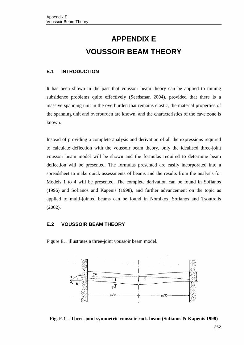
Appendix E Voussoir Beam Theory
352
APPENDIX E VOUSSOIR BEAM THEORY
E.1 INTRODUCTION
It has been shown in the past that voussoir beam theory can be applied to mining
subsidence problems quite effectively (Seedsman 2004), provided that there is a
massive spanning unit in the overburden that remains elastic, the material properties of
the spanning unit and overburden are known, and the characteristics of the cave zone is
known.
Instead of providing a complete analysis and derivation of all the expressions required
to calculate deflection with the voussoir beam theory, only the idealised three-joint
voussoir beam model will be shown and the formulas required to determine beam
deflection will be presented. The formulas presented are easily incorporated into a
spreadsheet to make quick assessments of beams and the results from the analysis for
Models 1 to 4 will be presented. The complete derivation can be found in Sofianos
(1996) and Sofianos and Kapenis (1998), and further advancement on the topic as
applied to multi-jointed beams can be found in Nomikos, Sofianos and Tsoutrelis
(2002).
E.2 VOUSSOIR BEAM THEORY
Figure E.1 illustrates a three-joint voussoir beam model.
Fig. E.1 – Three-joint symmetric voussoir rock beam (Sofianos & Kapenis 1998)
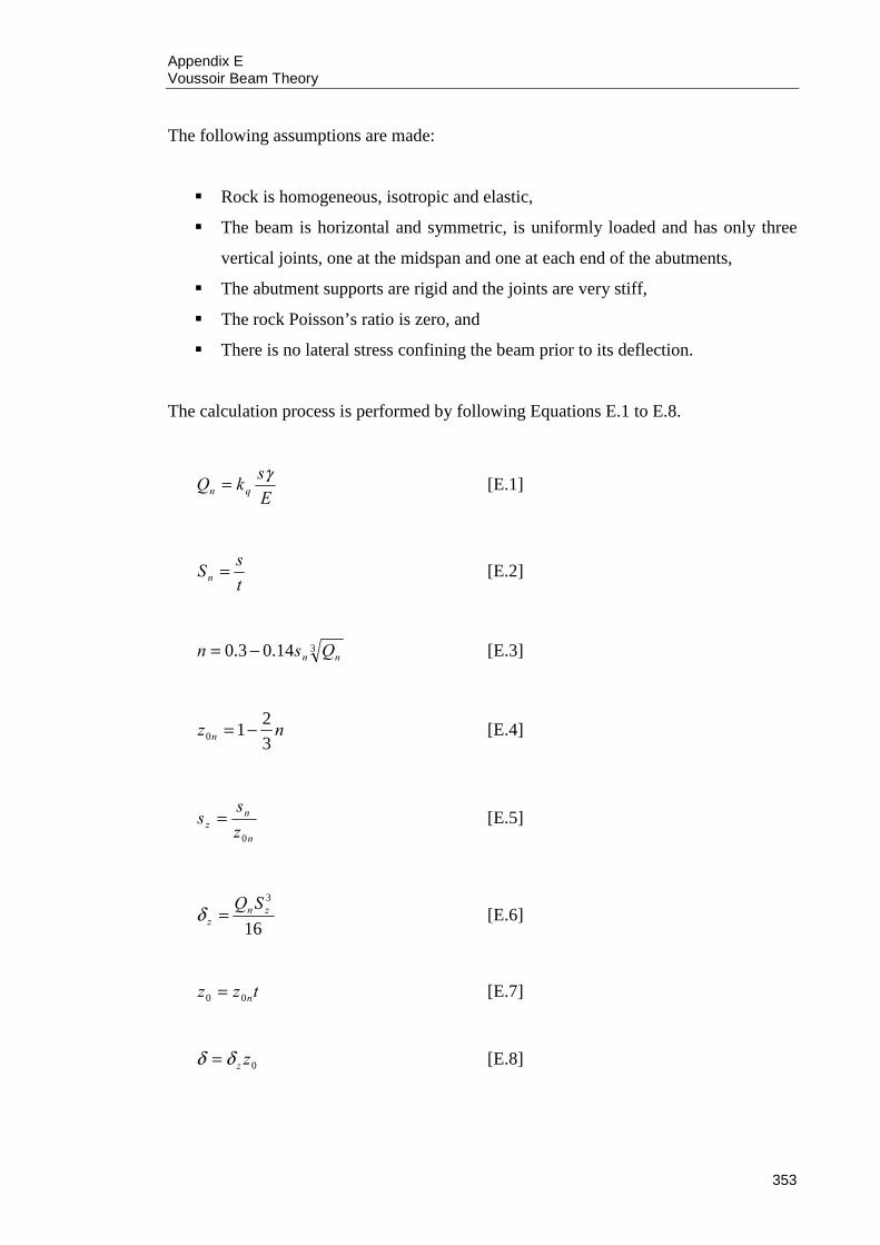
Appendix E Voussoir Beam Theory
353
The following assumptions are made:
Rock is homogeneous, isotropic and elastic,
The beam is horizontal and symmetric, is uniformly loaded and has only three
vertical joints, one at the midspan and one at each end of the abutments,
The abutment supports are rigid and the joints are very stiff,
The rock Poisson’s ratio is zero, and
There is no lateral stress confining the beam prior to its deflection.
The calculation process is performed by following Equations E.1 to E.8.
EskQ qnγ= [E.1]
tsSn = [E.2]
314.03.0 nn Qsn −= [E.3]
nz n 3210 −= [E.4]
n
nz z
ss
0
= [E.5]
16
3zn
zSQ
=δ [E.6]
tzz n00 = [E.7]
0zzδδ = [E.8]
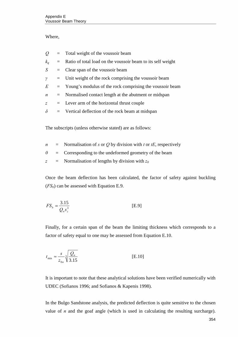
Appendix E Voussoir Beam Theory
354
Where,
Q = Total weight of the voussoir beam
kq = Ratio of total load on the voussoir beam to its self weight
S = Clear span of the voussoir beam
γ = Unit weight of the rock comprising the voussoir beam
E = Young’s modulus of the rock comprising the voussoir beam
n = Normalised contact length at the abutment or midspan
z = Lever arm of the horizontal thrust couple
δ = Vertical deflection of the rock beam at midspan
The subscripts (unless otherwise stated) are as follows:
n = Normalisation of s or Q by division with t or tE, respectively
0 = Corresponding to the undeformed geometry of the beam
z = Normalisation of lengths by division with z0
Once the beam deflection has been calculated, the factor of safety against buckling
(FSb) can be assessed with Equation E.9.
3
15.3
znb sQ
FS = [E.9]
Finally, for a certain span of the beam the limiting thickness which corresponds to a
factor of safety equal to one may be assessed from Equation E.10.
3
0min 15.3
n
n
Qzst ≈ [E.10]
It is important to note that these analytical solutions have been verified numerically with
UDEC (Sofianos 1996; and Sofianos & Kapenis 1998).
In the Bulgo Sandstone analysis, the predicted deflection is quite sensitive to the chosen
value of n and the goaf angle (which is used in calculating the resulting surcharge).

Appendix E Voussoir Beam Theory
355
Using an n value of 0.75 has proven to be effective whilst it has also been stated that for
a large number of joints, n is between 0.18 and 0.30 (Nomikos, Sofianos & Tsoutrelis
2002). The values of n used in the Bulgo Sandstone analysis have been calculated using
Equation E.3.