Computers and Geotechnics 75 (2016) 126–134

Contents lists available at ScienceDirect

Computers and Geotechnics

journal homepage: www.elsevier .com/ locate/compgeo

Research Paper

Numerical modelling of seismic slope failure using MPM

http://dx.doi.org/10.1016/j.compgeo.2016.01.0170266-352X/� 2016 Elsevier Ltd. All rights reserved.

⇑ Corresponding author at: Pfaffenwaldring 35, 70569 Stuttgart, Germany.E-mail addresses: bhandaritushar1390@gmail.com (T. Bhandari),

fursan.hamad@igs.uni-stuttgart.de (F. Hamad), christian.moormann@igs.uni-stuttgart.de (C. Moormann), kgsharmaiitd@gmail.com (K.G. Sharma),bmwest@gmx.de (B. Westrich).

1 Present address: SMEC India Pvt. Ltd., 5th Floor, Bldg. 8, Tower C, DLF Cyber CityPhase II, Gurgaon, Haryana, India.

Tushar Bhandari a,1, Fursan Hamad b, Christian Moormann b,⇑, K.G. Sharma a, Bernhard Westrich b

aDepartment of Civil Engineering, Indian Institute of Technology-Delhi, Hauz Khas, New Delhi, Indiab Institute of Geotechnical Engineering, University of Stuttgart, Stuttgart, Germany

a r t i c l e i n f o

Article history:Received 26 September 2015Received in revised form 12 December 2015Accepted 17 January 2016Available online 17 February 2016

Keywords:Material Point MethodNon-zero kinematic conditionLarge deformationLandslidesSlope failure

a b s t r a c t

The Finite Element Method (FEM) is widely used in the simulation of geotechnical applications. Owing tothe limitations of FEM to model problems involving large deformations, many efforts have been made todevelop methods free of mesh entanglement. One of these methods is the Material Point Method (MPM)which models the material as Lagrangian particles capable of moving through a background computa-tional mesh in Eulerian manner. Although MPM represents the continuum by material points, solutionis performed on the computational mesh. Thus, imposing boundary conditions is not aligned with thematerial representation. In this paper, a non-zero kinematic condition is introduced where an additionalset of particles is incorporated to track the moving boundary. This approach is then applied to simulatethe seismic motion resulting in failure of slopes. To validate this simulation procedure, two geotechnicalapplications are modelled using MPM. The first is to reproduce a shaking table experiment where theresults of another numerical method are available. After validating the present numerical scheme for rel-atively large deformation problem, it is applied to simulate progression of a large-scale landslide duringthe Chi-Chi earthquake of Taiwan in which excessive material deformation and transportation is takingplace.

� 2016 Elsevier Ltd. All rights reserved.

1. Introduction

Slopes stability has been considered as one of the most signifi-cant topic to study for the geotechnical society over many years. Inmost cases, the stability of slope is what one aims to analyse. Forthis reason, the evolution of analysis techniques has taken placein the regime of mesh based methods that can take into accountthe limiting deformations as well as the effect of supporting struc-tures. In some cases, however, it is important to study the beha-viour of the slopes beyond failure. In these cases, slope failure isinevitable and the impact of the sliding mass on low-lying areasbecomes important to investigate. The physical significance ofslope failures can be gauged in the form of landslides leading toa massive flow of debris. Landslide-debris flow is a very rapidand massive flow-like motion of soil and fragmented rock. Thematerial mobility and the impact of the avalanche can cause

significant damage to human life and engineering structures thatcome in the way of the flow.

Slope failures and landslides, in particular, can be triggered bymany factors including heavy rainfall, imposed loads, strengthdegradation due to weathering and seismic excitation. Amongthese factors, seismic excitation or earthquake has been recog-nised to be the major causes of slope failures [1]. Therefore itbecomes more important to analyse the response of a slope to aseismic event. Many methods have been developed to addressthis issue. Jibson [2] classifies the methods for assessing the per-formance of a slope during earthquakes fall into three phases: (1)pseudo static analysis, (2) permanent displacement analysis, and(3) stress–deformation analysis. Pseudo static analysis, used as apreliminary analysis method can only indicate the safety againstslope failure using a limit equilibrium method in which the seis-mic shaking is represented by a constant inertial force applied ona sliding mass. As a significant improvement to pseudo staticanalysis, permanent displacement analysis provides more quanti-tative measure to evaluate the performance of slopes duringearthquakes. A common example of the permanent displacementanalysis is the Newmark rigid-block analysis [3] where the per-manent slope deformation induced by earthquakes is estimatedby the permanent displacement of the rigid block sliding alongthe inclined plane under a base acceleration. Both pseudo static

Notations

q mass densityr the Cauchy stress tensorg gravitational acceleration vectoru displacementa nodal displacement vectore strain tensorX volumen unit normal vector

M mass matrixB gradient of the shape functionF nodal force vectorN shape function matrixC1 relaxation coefficientVp p-wave velocityvx horizontal component of velocityt time

T. Bhandari et al. / Computers and Geotechnics 75 (2016) 126–134 127

analysis and permanent displacement analysis are based onhighly simplified geometric and material models. However, thesemethods cannot be relied upon to evaluate earthquake-inducedslope deformations under complex geological conditions. For thispurpose, stress–deformation analysis is used which can accountfor complex soil behaviours (e.g., non-linear response to dynamicloading, strain softening and strain rate dependence of materialstrength) and geometric conditions. It follows the approach ofcomputing stresses in a material and its response in form ofdeformations based on a defined constitutive relationshipbetween stress and strain. A stress–deformation analysis is fre-quently performed using numerical methods like the Finite Ele-ment Method (FEM) or Finite Difference Method (FDM).However, the mesh based methods (e.g. FEM) have difficultiesin modelling large deformations due to problems of mesh distor-tion and entanglement. As a result, stress–deformation analysis iscurrently limited to estimating relatively small seismically-induced slope deformations [2]. The drawback of these methodsto deal with large deformations therefore considerably impedestheir application in the analysis of earthquake-induced slopedeformations.

In order to overcome these drawbacks in stress–deformationanalysis, various mesh-free methods have been proposed. TheMaterial Point Method (MPM) is one of these methods, whichhas shown its applicability to model granular materials like soilin different geotechnical applications [4,5]. Previous MPM researchhas focused on modelling of collapsing slopes and landslides usingstrength degradation [6]. Andersen and Andersen [7] also studiedcollapse of slopes in which the slide is initiated by increasing thedensity of material, corresponding to the behaviour during heavyrainfall. MPM has also been applied to model failure ofgeotextile-reinforced slope [8].

Although MPM represents the continuum by material points,solution is performed on the computational mesh. Thus, imposingboundary conditions is not aligned with the material representa-tion. A non-zero kinematic condition is introduced in this paperwhere an additional set of particles is incorporated to track themoving boundary. The MPM procedure is applied to simulatethe seismic excitation and dynamic response of a slope. The seis-mic history is introduced to the MPM model via the rigid bound-ary condition introduced by Hamad et al. [9,10]. Also, theproposed simulation approach is tested to model a shaking tableexperiment and to compare the results with correspondingnumerical simulation from Hiraoka et al. [11] using anothernumerical method called the Smooth Particle Hydrodynamics –SPH method. Finally, MPM is applied to simulate progression ofa large-scale landslide during the 1999 Chi-Chi earthquake of Tai-wan. In this paper, the effect of water is not considered. In manycases, water can be a triggering factor for landslides and mayimpact the simulation results significantly. However, the simula-tion of dry landslide can be very relevant in cases of dry debrisflow and rock avalanches where the controlling factor is theseismic motion.

2. Brief description of MPM

MPM can be viewed as an extension of the classical finite ele-ment procedure, in which the continuum body is discretised byLagrangian material points that can move through a fixed compu-tational mesh as shown in Fig. 1. The momentum equation issolved on the computational mesh which provides a convenientmeans of calculating discrete derivatives.

2.1. Spatial discretisation

We start with the conservation of linear momentum, whichreads

q€u ¼ r � rþ qg ð1Þwhere r(x, t) is the Cauchy stress tensor at position x and time t,q(x, t) is the mass density, g is the gravitational acceleration vector,u(x, t) is the displacement with the superposed dot denotingdifferentiation with time.

By taking the virtual displacement du as test function for adomain of volume X surrounded by boundary S, the weak formof the momentum equation can be written asZXduTq €udX ¼

ZXdeTrdXþ

ZXduTqgdXþ

ZCt

duTtdC ð2Þ

where t ¼ r � n is the prescribed traction on boundary Ct, n is theoutward unit normal and e is the strain tensor represented in vectorform. The superscript T denotes the transpose. Similar to the stan-dard finite element method, the value of a variable inside the ele-ment can be based on the nodal values and the nodal shapefunctions. Using these definitions and discretizing the momentumequation, it takes the form (e.g., [4])

M€a ¼ F ð3Þwhere M is the consistent mass matrix, €a the nodal accelerationvector, and (F = Fext–Fint) with Fext and Fint being the external andinternal nodal force vectors, respectively. In practice, the lumpedmass matrix is preferred over the consistent mass matrix. This sim-plifies the computations at the expense of introducing a slightamount of numerical dissipation [12]. Referring to Eq. (3), the inter-nal force vector is given by

Fint ¼Xnpp¼1

xpBTðxpÞrp ð4Þ

where the quotient of the material point mass and density is thevolume of the material point, xp =mp/qp and B is the gradient ofthe shape function, as also used in standard finite element method[4], rp is a vector containing the stress components at the materialpoint p. The external nodal force vector is given by

Fext ¼Xnpp¼1

mpNTðxpÞgþ

ZCt

NTtdC ð5Þ

Fig. 1. MPM representation of a continuum.

128 T. Bhandari et al. / Computers and Geotechnics 75 (2016) 126–134

where N is the global shape function matrix and np is the total num-ber of material points.

2.2. Time integration

The discretised momentum equation (Eq. (3)) needs to besolved for discrete time intervals. With the mass matrix being adiagonal matrix, the system of equations can be solved using theEuler-forward time integration scheme, i.e.

_atþDt ¼ _at þ Dt €at ; €at ¼ ½Mtl ��1

Ft ð6Þwhere Dt is the current time increment, _at and _atþDt are the nodalvelocities at time t and (t + Dt), respectively and Ml is the lumpedmass matrix. The incremental nodal displacement is obtained byintegrating the nodal velocity by the Euler-backward rule (see fore.g., Jassim et al. [13])

DatþDt ¼ Dt _atþDt ð7Þand the positions of the particles are subsequently updated from

xtþDtp ¼ xtp þ NpDatþDt ð8Þwhere xp

t and xpt +Dt are the particle positions at time t and (t + Dt)

respectively.For the present MPM solution procedure, a slightly different

algorithm has been adopted for updating the particles velocity fol-lowing Sulsky et al. [14]. By solving the equation of motion for thenodes, the elements deform and the material points in the interiorof the element move in proportion to the motion of the nodes,based on the nodal shape functions. The position of the materialpoints is updated using a single-valued continuous velocity fieldand hence the interpenetration of material is precluded. Thisautomatic feature of the algorithm allows simulations of no-slipcontact between different bodies without the need for specialinterface tracking and contact algorithms.

After getting the nodal velocities, the strain increment of amaterial point p is calculated. The constitutive model is appliedat the material points to get the incremental strain, which allowsdirect evaluation and tracking of history-dependent variables.

At the end of time step the material point variables are updatedand a new cycle begins using the information carried by the mate-rial points to initialise nodal values on the computational mesh.Note that at this stage, a new computational mesh can be definedsince all the state variables are carried by the material points. Inpractice, however, it is more efficient to use the original mesh.

2.3. Contact algorithm

The frictional contact algorithm proposed by Bardenhagen et al.[15] is used in this paper. It can be seen as a predictor–correctorscheme formulated in explicit manner, in which the velocity ispredicted from the solution of each body separately and then

corrected using the velocity of the coupled bodies followingCoulomb friction. This solution scheme uses the concept of com-paring the single and combined body velocities for a contact nodeand defining its behaviour accordingly. The algorithm is able todetect whether two bodies in contact are approaching orseparating from each other. If the two bodies are separating,the algorithm allows free separation where each body movesaccording to its own equation of motion. For more details aboutthe algorithm, the reader is referred to Ref. [15].

2.4. Prescribed velocity in MPM

In traditional dynamic FEM, the prescribed velocity is definedover nodes. These nodes always define part of the Lagrangian bodyboundary. On the other hand, in MPM the continuum is defined byLagrangian particles which might change position from one ele-ment to another. Hence, there is no defined interface surface whereprescribed velocity are applied.

Within the framework of MPM, prescribed velocity can beapplied directly on the material points of a rigid body representingthe moving boundary for simple one-dimensional problem. Forapplications with axial movement, part of the mesh can be dis-placed as a moving mesh having a prescribed value while the restis stretched uniformly [16]. This becomes very complicated andinconvenient when applied to applications like imposing seismicmotion for a slope problem. As an alternative, an additional setof particles (Fig. 2) is introduced which tracks the moving bound-ary by carrying the time-dependent boundary evolution [9]. Fol-lowing the same methodology, prescribed velocities are appliedas a boundary condition for the rigid wall and a contact is definedbetween the rigid wall and soil.

2.4.1. Non-zero kinematic conditionsIn this paper, the non-zero kinematic condition is developed as

shown in Fig. 2 where an additional set of particles is introduced,which tracks the moving boundary by carrying the time-dependent boundary evolution. At the beginning of a time step,the velocity _apðxp; tÞ of the prescribed particle p is assigned. Next,the prescribed velocity must be mapped (via the shape functions)from the prescribed particles to the computational nodes, wherethe discrete equations are solved. Nodes belonging to the elementswhere the prescribed particles are located are then tagged to beboundary nodes. It should be appreciated that the thickness ofthe boundary corresponds to one computational element. The pre-scribed values are assigned directly at the boundary nodes. As analternative, a weighted mapping procedure can be used, which ismore consistent with the principles of MPM, with the nodal veloc-ity _ai of boundary node i being obtained from [9,10]

_ai ¼P

pNiðnpÞwp _apPpNiðnpÞwp

ð9Þ

where _ap is the prescribed velocity of material point p, Ni(np) is theshape function of i being evaluated at p, and wp is a weighting func-tion (e.g. mass or volume of p). The summations in this equation runover the number of prescribed particles. Depending on the locationof the boundary particles, the number of the boundary nodes isupdated constantly as well as their values from Eq. (9).

2.4.2. Validation case: prescribed velocity with contactTo validate the procedure of introducing prescribed velocity

particles involving contact, a (1 � 1 m) square with a unit weightof 10 kN/m3 supported by 45 prescribed particles with zerovelocity is considered. After calculating the initial gravitationalstresses, the layer of prescribed particles underneath is movedsuddenly with a horizontal velocity of 2 m/s. Fig. 3 shows three

Soil

(a) Two Bodies in Contact

Contact InterfacePrescribed Velocity

(b) MPM Representation

Frictional Contact

Rigid Wall

Fig. 2. Prescribed velocity in MPM.

1.0 m

45o

0.35 0.53

1

2

Wall

Shaking Table

0.5

0.9

0.2

45o

1

2

Fig. 4. Experimental model (after Hiraoka et al. [11]).

T. Bhandari et al. / Computers and Geotechnics 75 (2016) 126–134 129

scenarios: if the standard MPM (top) is applied, the body travelstogether with the bottom; for the case where a rough contact isintroduced (middle), the glue condition is broken if the bottommoves fast enough; finally, the absence of the frictional resistancein the smooth contact case (bottom) leads to the early separationof the two bodies as shown.

3. Numerical application

In the geotechnical field, dynamic process of slope failures sub-jected to seismic loads is often investigated by means of physicalmodelling [17–19]. Slope failure under seismic excitation is imple-mented by a box filled with soil and mounted on a shaking table.These experiments play a vital role in the calibration of numericalmodels for similar applications. For assessing the performance ofMPM to simulate seismic excitation in geo-mechanical problems,a shaking table experiment is considered here and the simulatedresponse is compared with published results [11] based on SmoothParticle Hydrodynamics (SPH) method. The objective here is to testthe proposed numerical scheme in MPM (including the non-zerokinematic condition) with a simple Mohr–Coulomb failure crite-rion for simulating a dynamic test in comparison with more estab-lished numerical methods like SPH.

Fig. 3. Prescribed velocity boundary with contact: (top) standard

The shaking table experiment under consideration consists of asmall-scale cut slope as shown in Fig. 4. A steel box is mounted ontop of the shaking table. The soil slope model (0.9 � 0.6 � 0.5 m)was set in the shaking box, and the slope angle was made as 45�.The soil used in the experiment was Masa soil which is weatheredgranite commonly found in Kansai area in Japan. Laser displace-ment sensors were used to measure displacement within the slope.The slope model was subjected to the seismic wave loading shownin Fig. 5. The test runs for 14 s until the slope completely collapsed.More details about the test setup and the experiment can be foundin Ref. [11].

3.1. Reference solutions

In order to test the proposed treatment of boundary conditionsin MPM, a comparison with other numerical methods namely theFinite Element Method (FEM) and the Smooth Particle Hydrody-namics (SPH) method is provided in this paper. The FEM modelused in this research is suitable for the failure initiation wheresmall deformation theory is applicable. On the other hand, theSPH model is more appropriate for the large deformation analysis.

MPM, (middle) rough contact, and (bottom) smooth contact.

-0.15-0.10-0.050.000.050.100.15

0 2 4 6 8 10 12 14

Vel

ocity

, vx

(m/s

)

Time (s)

Fig. 5. Velocity–time history of the shaking table (after Hiraoka et al. [11]).[%]1.5

0

Fig. 6. Finite element analysis at t = 10 s: (top) deformed mesh and (bottom) shearstrain.

130 T. Bhandari et al. / Computers and Geotechnics 75 (2016) 126–134

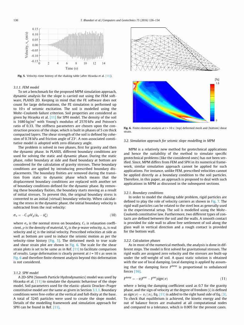
3.1.1. FEM modelTo set a benchmark for the proposed MPM simulation approach,

dynamic analysis for the slope is carried out using the FEM soft-ware, PLAXIS 2D. Keeping in mind that the FE software does notcount for large deformations, the FE simulation is performed upto 10 s of seismic excitation. The soil is modelled using theMohr–Coulomb failure criterion. Soil properties are considered asgiven by Hiraoka et al. [11] for SPH model. The density of the soilis 1680 kg/m3 with Young’s modulus of 2570 kPa and Poisson’sratio of 0.33. The stiffness parameters are chosen upon the con-struction process of the slope, which is built in phases of 5 cm thickcompacted layers. The shear strength of the soil is defined by cohe-sion of 0.78 kPa and friction angle of 23�. A non-associated consti-tutive model is adopted with zero dilatancy angle.

The problem is solved in two phases, first for gravity and thenthe dynamic phase. In PLAXIS, different boundary conditions areused for solving the static and dynamic phase. During the staticphase, roller boundary at side and fixed boundary at bottom areconsidered for the calculation of gravity stresses. These boundaryconditions are applied by introducing prescribed boundary dis-placements. The boundary fixities are removed during the transi-tion from static to dynamic phase which means that thedisplacement boundary conditions are replaced with another setof boundary conditions defined for the dynamic phase. By remov-ing these boundary fixities, the boundary starts moving as a resultof initial stresses. To prevent this, the original boundary stress isconverted to an initial (virtual) boundary velocity. When calculat-ing the stress in the dynamic phase, the initial boundary velocity issubtracted from the real velocity:

rn ¼ �C1qVpð _un � _uonÞ ð10Þ

where rn is the normal stress on boundary, C1 is relaxation coeffi-cient, q is the density of material, Vp is the p-wave velocity, _un is realvelocity and _uo

n is the initial velocity. Prescribed velocities at side aswell as bottom are used to induce the seismic motion as per thevelocity–time history (Fig. 5). The deformed mesh to true scaleand shear strain plot are shown in Fig. 6. The scale for the shearstrain plots is set to be same as in Ref. [11] to facilitate comparisonof results. Large deformation is clearly present at t = 10 s as seen inFig. 6 and therefore finite element analysis beyond this deformationis not considered.

3.1.2. SPH modelA 2D-SPH (Smooth Particle Hydrodynamics) model was used by

Hiraoka et al. [11] to simulate the dynamic behaviour of the slopemodel. Soil parameters used for the elastic–plastic Drucker–Pragerconstitutive model are the same as given in Section 3.1.1. Boundaryconditions were free-roller at the vertical and full-fixity at the base.A total of 3245 particles were used to create the slope model.Details of the modelling framework and simulation approach forSPH can be found in Ref. [11].

3.2. Simulation approach for seismic slope modelling in MPM

MPM is a relatively new method for geotechnical applicationsand hence the suitability of the method to simulate specificgeotechnical problems (like the considered ones) has not been ver-ified. Since, MPM differs from FEM and SPH in its numerical frame-work, similar simulation approach cannot be applied for suchapplications. For instance, unlike FEM, prescribed velocities cannotbe applied directly as a boundary condition to the soil particles.Therefore, in this paper, an approach is proposed to deal with suchapplications in MPM as discussed in the subsequent sections.

3.2.1. Boundary conditionsIn order to model the shaking table problem, rigid particles are

defined to play the role of velocity carriers as shown in Fig. 7. Therigid wall particles can be related to the steel box as generally usedin the experimental setup. The soil is modelled using the Mohr–Coulomb constitutive law. Furthermore, two different types of con-tacts are defined between the soil and the walls. A smooth contactis provided for side wall to allow free settlement of soil along theglass wall in vertical direction and a rough contact is providedfor the bottom wall.

3.2.2. Calculation phasesAs in most of the numerical methods, the analysis is done in dif-

ferent steps. The model is first solved for gravitational stresses. Therigid walls are assigned zero velocity and the stresses are built-upunder the self-weight of soil. A quasi static solution is obtainedwith the use of local damping. Local damping is applied by assum-

ing that the damping force Fdamp is proportional to unbalancedforces [16].

Fdamp ¼ �ajFext � F intjsignðvÞ ð11Þwhere a being the damping coefficient used as 0.7 for the gravityphase, and the sign of velocity at the degree of freedom (i) is definedas signðvÞ ¼ v i=jv ij. Eq. (11) is added to the right hand side of Eq. (3).To check that equilibrium is achieved, the kinetic energy and theout of balance forces are evaluated at all computational nodesand compared to a tolerance, which is 0.005 for the present cases.

Smooth contact µ=0

Rough contact µ=1

vx(t)= prescribed velocity (Fig. 5) vy(t)= 0

Rigid Particle

M-C Soil

Fig. 7. Dynamic boundary conditions in MPM.

M-C Soil

Rigid Wall

Fig. 8. Initial configuration of the MPM model.

[%]1.5

0

[m]

0.21

T. Bhandari et al. / Computers and Geotechnics 75 (2016) 126–134 131

After obtaining an equilibrium state of gravity stresses, nextstep for calculation is defined for dynamic analysis. The localdamping is switched off and prescribed velocities (Fig. 5) areassigned to the rigid walls which simulates dynamic motion ofthe steel box and consequent behaviour of the soil it contains tak-ing into account the external forces, body forces and the inertialforces.

0

Fig. 9. MPM analysis: (top) shear strain at t = 10 s and (bottom) norm of totaldisplacement at t = 14 s.

3.2.3. Simulated resultsTo model the seismic excitation of the soil slope in MPM, the

simulation approach as discussed in Sections 3.2.1 and 3.2.2 isused. Mesh and particle discretisation are illustrated in Fig. 8.Shear strain at t = 10 s and total displacement at t = 14 s are shownin Fig. 9.

The dynamic response of the slope can be described in the formof displacement history of specific points on the slope. The dis-placement histories of specific control points 1 and 2 as outlinedin Fig. 4 are used to compare the experimental results with thedynamic response predicted by different numerical models. Thecomparison for the vertical displacement history for point 1 andhorizontal displacement history for point 2 are shown in Fig. 10.It is evident that even with limited time i.e. t = 10 s, FEM in unableto predict the trend of deformations towards failure. The deforma-tion behaviour of the slope as predicted by MPM is in fair compar-ison with that predicted by SPH and also close to the experimentalresults. Sensitivity of the analysis results to mesh discretizationwas also assessed by solving three cases for different mesh sizes.The details of these cases are presented in Appendix A. It is notedthat like other mesh based methods, MPM results are also depen-dent on the size of mesh. With a variation of ±60% in the mesh size,the maximum total displacement varies up to around ±7%.

In the present analyses, the shape of the sliding surface is pre-dicted as almost circular, which is in agreement with the othercontinuum-based model using SPH. However, the sliding surfaceas observed from the experiment was a curved line with highercurvature angle. Hiraoka et al. [11] suggest a lack of clarity aboutthis failure mechanism observed in the experiment and attributeit to possible technical errors while removing the collapsing soilto specify the failure surface in the experiments. The SPH analysis[11] also suggests to assign a non-zero dilatancy angle (w = //2 and/) in order to come closer to the experiment. Although thisassumption improves the prediction of the failure surface, itover-predicts the plastic volumetric expansion like the soil is heav-ily compacted which contradicts the initial state of the considered

soil. Consequently, large run-out distance is observed in thenumerical model. Therefore, these analyses are excluded from thispaper.

Advanced constitutive models that consider the effect of soildegradation with the stress and density evolutions are supposedto perform better than the simple elasto-plastic Mohr–Coulombmodel being used. In principle, the implementation of these mod-els in MPM is straightforward, while the related numerical stabilityproblems are under study and the formulation under development.Considering that the soil in the experiment is reported to have 10%water content, the advanced constitutive model should be com-bined with partially saturated soil model for better simulation ofthe progressive failure of the experiment.

4. Earthquake induced landslide debris flow

The dynamic process of landslides induced by earthquakes isvery complex in its nature. Various numerical methods are usedto simulate different activities involved in the whole process ofevolution of a landslide starting from the development of a criticalsliding surface to initiation and triggering of failure to disintegra-tion of the sliding mass to debris flow and finally deposition. In thissection, MPM is used to simulate the last part of the process i.e.progression of the sliding mass and deposition. For this, theChiu-fen-erh-shan landslide of 1999 is used as a case studyexample.

-150

-125

-100

-75

-50

-25

00 2 4 6 8 10 12 14

Ver

tical

Dis

plac

emen

t (m

m)

Time (s)

Experimental SPH

PLAXIS MPM

0

50

100

150

200

0 2 4 6 8 10 12 14

Hor

izon

tal D

ispl

acem

ent (

mm

)

Time (s)Experimental SPHPLAXIS MPM

Fig. 10. Displacement history of the control points: (top) Point 1 and (bottom)Point 2.

Pre-slide TopographyPost-slide Topigraphy

500 (m)

Fig. 11. Topography of landslide (after Wu et al. [23]).

-0.4-0.20.00.20.40.60.81.0

0 20 40 60 80 100

Vel

ocity

, vx

(m/s

)

Time (s)

Fig. 12. Time history of the horizontal velocity (after Wu et al. [23]).

Fig. 13. Progression of landslide.

132 T. Bhandari et al. / Computers and Geotechnics 75 (2016) 126–134

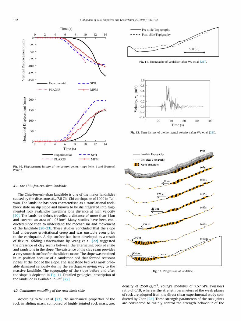
4.1. The Chiu-fen-erh-shan landslide

The Chiu-fen-erh-shan landslide is one of the major landslidescaused by the disastrousMw 7.6 Chi-Chi earthquake of 1999 in Tai-wan. The landslide has been characterised as a translational rock-block slide on dip slope and known to be disintegrated into frag-mented rock avalanche travelling long distance at high velocity[20]. The landslide debris travelled a distance of more than 1 kmand covered an area of 1.95 km2. Many studies have been con-ducted since then to understand the mechanism and movementof the landslide [20–23]. These studies concluded that the slopehad undergone gravitational creep and was unstable even priorto the earthquake. A slip surface had been developed as a resultof flexural folding. Observations by Wang et al. [22] suggestedthe presence of clay seams between the alternating beds of shaleand sandstone in the slope. The existence of the clay seam providesa very smooth surface for the slide to occur. The slope was retainedin its position because of a sandstone bed that formed resistantridges at the foot of the slope. The sandstone bed was most prob-ably damaged seriously during the earthquake giving way to themassive landslide. The topography of the slope before and afterthe slope is depicted in Fig. 11. Detailed geological description ofthe landslide is available in Ref. [22].

4.2. Continuum modelling of the rock-block slide

According to Wu et al. [23], the mechanical properties of therock in sliding mass, composed of highly jointed rock mass, are:

density of 2550 kg/m3, Young’s modulus of 7.57 GPa, Poisson’sratio of 0.19, whereas the strength parameters of the weak planesof rock are adopted from the direct shear experimental study con-ducted by Chen [24]. These strength parameters of the rock jointsare considered to mainly control the strength behaviour of the

[%]1.5

0

[%]1.5

0

[%]1.5

T. Bhandari et al. / Computers and Geotechnics 75 (2016) 126–134 133

sliding mass as movement is likely to occur along the existingweak planes in the sliding mass and thus these parameters areused directly to define the shear strength of the continuum. Thevalues adopted for the cohesion and friction are 20 kPa and 24�respectively.

In the present numerical scheme, the aim is to model the rockjoint masses as a continuum material. Therefore, the elastic modu-lus of the equivalent medium was estimated to be 500 MPa with ageological strength index range of 25–30 [25].

4.3. Material point analysis of the landslide

For the seismic motion, horizontal component of the velocity–time history of the Chi-Chi earthquake as shown in Fig. 12 wasused. This history was used by Wu et al. [23] in their discrete anal-ysis using velocities projected to the slope direction and correctedfor baseline correction. The sliding surface in MPM is modelledusing rigid particles and the velocities are imposed on theseparticles.

4.4. Simulated results

The progression of the flow resulting from the landslide isdepicted in Fig. 13. The progressive displacement of the front of

Table A.1Discretization details for cases of mesh sensitivity analysis.

S. no. Item Case-1 Case-2 Case-3

1. Number of particles 101,100 47,640 24,5402. Number of elements 16,174 7503 40293. Number of nodes 32,827 15,336 83154. Average element size 1.05 � 10�3 m 1.89 � 10�3 m 2.97 � 10�3 m

Fig. A.1. Mesh and particle discretization for cases 1, 2 and 3 (top to bottom).

0

Fig. A.2. Shear strain at t = 10 s for cases 1, 2 and 3 (top to bottom).

the sliding mass is marked for different time steps. It can be seenfrom the stabilizing displacement profile that the sliding massreaches an equilibrium state in 120 s. The final configuration assimulated by MPM is compared with the actual scenario inFig. 13 which suggests a fair match between the shape of the debrisdeposit except for a slightly different shape at the rare end of thedebris flow.

5. Conclusion and outlook

An important geotechnical application has been modelled usingthe MPM. Simulation approach to induce seismic motion in MPM istested by modelling a shaking table experiment and comparing theresults with other numerical methods. The deformation behaviourof the slope as predicted by MPM is in fair comparison with thatpredicted by SPH. A variation of the order of 5% in results isobserved and attributed to the fact that both MPM and SPH differin their basic formulation. Also, the failure criteria and implemen-tation of boundary conditions used in both the methods are differ-ent. Compared to SPH, MPM is seen to predict the dynamicresponse of the slope closer to the experimental results. However,better simulation of progressive failure can be achieved by incor-porating advanced constitutive models in the current formulationof MPM. The limitation of conventional FEM to model large defor-mation problems is also emphasised by comparing the results withFEM simulation using PLAXIS. While this limitation can largely beovercome by Lagrangian–Eulerian methods, remeshing may still berequired and state variables associated with material points needto be remapped. This is of particular concern when the history ofthe material must be taken into account.

[m]0.23

0

[m]0.21

0

[m]0.20

0

Fig. A.3. Total displacement at t = 14 s for cases 1, 2 and 3 (top to bottom).

134 T. Bhandari et al. / Computers and Geotechnics 75 (2016) 126–134

Finally, the potential of the MPM to model extensivedeformation in form of landslide debris-flow is demonstrated.MPM is seen to simulate the progression of the landslide andgenerate a reasonable post-failure configuration. The proposedsimulation approach holds well for the post failure scenariobut detailed study is required to understand the modelling ofcomplete evolution process of landslides which may include abetter contact algorithm to model the brittle behaviour of rockjoints and precise equivalent continuum modelling of rock mass.Moreover, the present approach can be extended with furtherstudies to include the effect of water and improve constitutivemodelling to take into account the behaviour of rock in dynamicconditions.

Acknowledgements

The authors acknowledge the help of ‘‘German AcademicExchange Service (DAAD)” and ‘‘Institute of Geotechnical Engineer-ing (IGS), Stuttgart” for providing the financial and physicalresources required to carry out this research. We would also liketo acknowledge ‘‘Deltares, The Netherlands” for providing accessto their MPM source code, which was further developed in thispaper.

Appendix A

To assess the sensitivity of the model to mesh discretization,three cases for different mesh sizes were solved. The discretizationdetails of these cases are presented in Table A.1.

The mesh for the three cases is shown in Fig. A.1. Analysisresults in form of contour plots for shear strain at t = 10 s and totaldisplacement at 14 s are presented in Figs. A.2 and A.3 respectivelyfor the three cases.

References

[1] Keefer DK. Landslides caused by earthquakes. Geol Soc Am Bull 1984;95(4):406–21.

[2] Jibson RW. Methods for assessing the stability of slopes during earthquakes – aretrospective. Eng Geol 2011;122(1):43–50.

[3] Newmark NM. Effects of earthquakes on dams and embankments.Geotechnique 1965;15(2):129–60.

[4] Wieckowski Z, Youn S-K, Yeon J-H. A particle-in-cell solution to the silodischarging problem. Int J Numer Meth Eng 1999;45(9):1203–25.

[5] Coetzee C, Vermeer P, Basson A. The modelling of anchors using the materialpoint method. Int J Numer Anal Meth Geomech 2005;29(9):879–95.

[6] Andersen S, Andersen L. Modelling of landslides with the material-pointmethod. Comput Geosci 2010;14(1):137–47.

[7] Andersen S, Andersen L. Material-point-method analysis of collapsing slopes.In: Proceedings of the 1st international symposium on computationalgeomechanics (ComGeo I), Juan-les-Pins, France; 2009. p. 817–28.

[8] Hamad F, Vermeer P, Moormann C. Failure of a geotextile-reinforcedembankment using the material point method. In: Proceedings of the 3rdinternational conference on particle-based methods-fundamentals andapplications, Stuttgart, Germany; 2013. p. 498–509.

[9] Hamad F, Vermeer P, Moormann C. Development of a coupled FEM-MPMapproach to model a 3D membrane with an application of releasinggeocontainer from barge. In: Proceedings of the 3rd international conferenceon installation effects in geotechnical engineering, Rotterdam, TheNetherlands; 2013. p. 176–83.

[10] Hamad F, Stolle D, Moormann C. Material point modelling of releasinggeocontainers from a barge. J Geotext Geomembranes 2016;44(3):308–18.

[11] Hiraoka N, Oya A, Bui HH, Rajeev P, Fukagawa R. Seismic slope failuremodelling using the Mesh-free SPH method. Int J GEOMATE 2013;5:660–5.

[12] Burgess D, Sulsky D, Brackbill J. Mass matrix formulation of the FLIP particle-in-cell method. J Comput Phys 1992;103(1):1–15.

[13] Jassim I, Stolle D, Vermeer P. Two-phase dynamic analysis by material pointmethod. Int J Numer Anal Meth Geomech 2013;37(15):2502–22.

[14] Sulsky D, Zhou S-J, Schreyer HL. Application of a particle-in-cell method tosolid mechanics. Comput Phys Commun 1995;87(1):236–52.

[15] Bardenhagen S, Brackbill J, Sulsky D. The material-point method for granularmaterials. Comput Methods Appl Mech Eng 2000;187(3):529–41.

[16] Jassim I, Hamad F, Vermeer P. Dynamic material point method withapplications in geomechanics. In: Proceedings of the 2nd internationalsymposium on computational geomechanics (COMGEO II), Cavtat-Dubrovnik, Croatia; 2011. p. 445–6.

[17] Kutter BL. Earthquake deformation of centrifuge model banks. J Geotech Eng1984;110(12):1697–714.

[18] Arulanandan K, Yogachandran C, Muraleetharan K, Kutter B, Chang G.Seismically induced flow slide on centrifuge. J Geotech Eng 1988;114(12):1442–9.

[19] Wartman J, Seed RB, Bray JD. Shaking table modeling of seismically induceddeformations in slopes. J Geotech Geoenviron Eng 2005;131(5):610–22.

[20] Huang C-C, Lee Y-H, Liu H-P, Keefer DK, Jibson RW. Influence of surface-normalground acceleration on the initiation of the Jih-Feng-Erh-Shan landslide duringthe 1999 Chi-Chi, Taiwan, earthquake. Bull Seismol Soc Am 2001;91(5):953–8.

[21] Hung J-J. Chi-Chi earthquake induced landslides in Taiwan. Earthq Eng EngSeismol 2000;2(2):25–33.

[22] Wang W-N, Chigira M, Furuya T. Geological and geomorphological precursorsof the Chiu-fen-erh-shan landslide triggered by the Chi-chi earthquake incentral Taiwan. Eng Geol 2003;69(1):1–13.

[23] Wu J-H, Lin J-S, Chen C-S. Dynamic discrete analysis of an earthquake-inducedlarge-scale landslide. Int J Rock Mech Min Sci 2009;46(2):397–407.

[24] Chen H. Engineering geological characteristics of Taiwan landslides. Sino-Geotechnics 2000;79:59–70.

[25] Hoek E, Diederichs MS. Empirical estimation of rock mass modulus. Int J RockMech Min Sci 2006;43(2):203–15.