numerical modelling of seismic waves scattered by hydrofractures

$: Numerical modelling of seismic waves scattered by hydrofractures$
Numerical modelling of seismic waves scattered by hydrofractures:application of the indirect boundary element method

Tim Pointer,1,* Enru Liu1 and John A. Hudson2

1 Global Seismology and Geomagnetism Group, British Geological Survey, West Mains Road, Edinburgh, EH9 3LA, UK2 Department of Applied Mathematics and Theoretical Physics, University of Cambridge, Silver Street, Cambridge, CB3 9EW, UK

Accepted 1998 June 1. Received 1998 May 18; in original form 1998 February 5

SUMMARYWe use a numerical method that can model the seismic waveforms scattered from anarbitrary number of fractures that are either empty, or contain elastic or £uid material.The indirect boundary element method (BEM) is capable of generating the full elasticwave¢eld and is programmed in two dimensions. The governing equations and discreteimplementation of the technique are described.We explain in detail a new approach forevaluating the improper boundary integrals.

The method is shown to be highly accurate from a comparison with modesummation. Subsequently, the BEM is applied to modelling hydrofractures. Syntheticexamples, calculated for cross-well and single-well geometries, demonstrate thee¡ects of crack length, opening and in¢ll on recorded displacements. It is shown thatdi¡ractions from the tips can, in principle, be used to locate and determine the hydro-fracture size. These arrivals depart from ray theoretical traveltimes due to defocusingover a Fresnel zone. S-wave di¡ractions generally have a larger amplitude than thedi¡racted P waves, and so may provide a better indication of fracture size. Energythat is converted to interface waves and subsequently di¡racted from the crack tipsis also observed. The presence of water allows energy to pass through the fracture;this is clearly evident on the cross-well seismograms. Closure of the fracture causes afurther increase in transmission amplitude as less energy is attenuated through internalmultiples.

Key words: boundary element method, crack tip di¡raction, hydrofracture,improper integral, interface waves.

1 INTRODUCTION

The motivation for analysing time-dependent seismic data isto understand how temporal changes in the elastic wave-¢eld can be generated by external in£uences such as thosethat occur during improved oil recovery (IOR). Modellingthe seismic response produced during a hydraulic fracturingtreatment is of particular interest: hydrofracturing is theprimary means of increasing the hydrocarbon production froma well (Vinegar et al. 1992). Ideally, if it were possible todetermine the location, dimensions and in¢ll of the hydro-fracture throughout the treatment then the e¤cacy of theproduction programme could be optimized accordingly.The modelling of seismic waves scattered by cracks

or fractures has taken a variety of approaches. Analyticalsolutions for the di¡racted seismic wave¢eld produced by

a fracture are only available for single cracks with a simplegeometry (Mal 1970), and in some cases are only valid inthe far ¢eld (Liu, Crampin & Hudson 1997) . Seismologistshave to employ numerical approaches in order to simulatethe di¡racted wave¢eld produced by models that approachanything like the real scenario.Each method has inherent advantages and disadvantages.

In some techniques simpli¢cations or approximations to therepresentation of the elastic wave¢eld are invoked to reducememory requirements and computation time so that complexmodels can be considered. Other methods can synthesize thefull wave¢eld but the investigator is limited to using a muchsimpler parametrization. With the advent of powerful parallelcomputers more researchers are starting to adopt the latterapproach. The techniques employed so far to study seismicwave scattering problems include Maslov theory (Chapman& Drummond 1982), the ¢nite di¡erence method (Fehler& Aki 1978), the ¢nite element method (Lysmer & Drake1972), the Born approximation (Wu & Aki 1985), the complex-screen approach (Wu 1994), Kirchho¡^Helmholtz integration

*Now at: BG Technology, Gas Research and Technology Centre,Ashby Road, Loughborough, Leicestershire, LE11 3GR, UK.E-mail: [email protected]

Geophys. J. Int. (1998) 135, 289^303

ß 1998 RAS 289

GJI000 14/9/98 13:08:23 3B2 version 5.20The Charlesworth Group, Huddersfield 01484 517077

Dow

nloaded from https://academ

ic.oup.com/gji/article-abstract/135/1/289/570126 by guest on 04 April 2019

(Neuberg & Pointer 1995), the boundary integral equationmethod (Benites, Aki & Yomogida 1992) and the boundaryelement method (BEM) (Chen & Zhou 1994).An indirect BEM is used in this paper. The main advantage

is that an integral representation of the elastic wave¢eldallows one to model fractures with an arbitrary shape. Thecomplete wave¢eld is produced, including all multiples andreverberations, and in fact the only approximation involvedis the discretization of the crack surface into a number of linearelements. To keep computation times to within reasonablelimits, the implementation is in two dimensions, and there-fore the analysis is restricted to modelling the cross-section ofa hydrofracture.In the following section the governing equations and

implementation of the BEM are examined, and the advantagesand disadvantages of using this approach are made apparent.A comparison is made with analytical solutions. This isfollowed by synthetic examples that show the e¡ects on thedi¡racted radiation pattern of di¡erent crack geometries andin¢lls. Salient features that may be evident in ¢eld data areexamined.This leads on to a ¢nal discussion and some remarks.

2 GOVERNING EQUATIONS ANDDISCRETE IMPLEMENTATION

The BEM approach to solving physical problems is based uponformulating the governing expressions in terms of boundaryintegral equations. The derivation of the background theoryhas been carried out in similar forms by Banerjee & Butter¢eld(1981), Bonnet (1989), Coutant (1989) and Sanchez-Sesma &Campillo (1991), and is explained clearly in Appendix A.

Elastic inclusions

Consider an exterior unbounded (E) region, DE, within whichthere is a source of elastic radiation, and an interior (I) region,DI, surrounded by a surface S (Fig. 1). The total displacementwave¢eld u(t) in the exterior region at a point x consists of twoparts: (i) a known incident wave u(i) due to the source alone,and (ii) a di¡racted wave u(d); it can be expressed as

u(t)j (x)~u(i)j (x)zu(d)j (x) . (1)

The total wave¢eld in the interior region comprises therefracted displacements

u(t)j (x)~u(r)j (x) . (2)

Similar expressions can be written for the tractions both insideand outside the inclusions.The boundary conditions on S are the continuity of

displacement and traction. Therefore, we can equate (1) and(2) and the corresponding expressions for the tractions atall points of S as expressed by eqs (A13). We now sub-stitute discrete versions of eqs. (A8), (A9) and (A12) for thedi¡racted and refracted displacements and tractions andobtain the following:

XMl~1

GEjk(xm, jl)�

Ekl{

XMl~1

GIjk(xm, jl)�

Ikl~{u(i)j (xm) , m~1, M ,

XMl~1

TEjk(xm, jl)�

Ekl{

XMl~1

TIjk(xm, jl)�

Ikl~{t(i)j (xm) , m~1, M.

(3)

To achieve this, the surface S has been discretized into Mlinear elements of size *Sl (l~1, 2, . . . , M). Expression (3)represents a system of linear equations for the unknownquantities �Ekl~�Ek (jl)*Sl and �Ikl~�Ik(jl)*Sl (l~1, 2, . . . , M).On the right-hand side are the incident displacements u(i) andtractions t(i) at the midpoints xm of the surface elements onthe boundary S (Fig. 1). The incident wave¢eld is that whichwould exist in the absence of any scattering surfaces, and canbe calculated analytically using for example an expression fora plane wave propagating from in¢nity or a moment tensordescription of a point source.The kernels in (3) consist of (i) G

Ejk(xm, jl) and G

Ijk(xm, jl),

the displacement Green's functions for the lth elementcorresponding to the exterior and interior regions, respectively,and (ii) TE

jk(xm, jl) and TIjk(xm, jl), the traction Green's tensors

for the lth element. They can be calculated using

Gjk(xm, jl)~�

*Sl

Gjk(xm, j)dsj (4)

and

Tjk(xm, jl)~+12

djkdmlz

�*Sl

Tjk(xm, j)dsj , (5)

where Gjk and Tjk are, respectively, the displacement andtraction Green's functions, and the z/{ signs correspondto the interior and exterior regions respectively. Ourimplementation is in 2-D isotropic media, so P^SV and SHmotions are decoupled. The full-space Green's functions areemployed and are given in Appendix B. They can also becalculated numerically using the discrete wavenumber method(Bouchon 1987). The simultaneous equations (3) are validfor three dimensions (Sanchez-Sesma & Luzon 1995) and fullanisotropy (Wang, Achenbach & Hirose 1996) providing Gjk

and Tjk can be evaluated.Integrals (4) and (5) can be calculated by numerical means,

such as Gaussian quadrature (Press et al. 1992). There is asingularity in both the displacement and the traction Green'sfunctions where the load point jl coincides with the ¢eld pointxm (Appendix C). Closed-form solutions for the displacementintegration in two dimensions have been given recently byTadeu, Kausel & Vrettos (1996). The singularity in displace-ment is logarithmic (see eq. C2) and therefore weak, so wesimply integrate as usual over the element with midpoint jl in

Figure 1. Problem con¢guration for the indirect BEM. The totalwave¢eld u(t) in the exterior region DE is the sum of the incidentwave¢eld u(i) generated by the source and the scattered wave¢eld u(d).


ß 1998 RAS, GJI 135, 289^303

290 T. Pointer, E. Liu and J. A. HudsonD

ownloaded from

https://academic.oup.com

/gji/article-abstract/135/1/289/570126 by guest on 04 April 2019

our code. However, the singularity in traction is of the form 1/r(see eq. C4), where r~jxm{jl j, and cannot be integrated over.Integral (5) is, therefore, improper (Appendix C) and mustbe understood as a Cauchy Principal Value integral, wherebythe second term on the right-hand side is null if m~l, as thelimiting form is an odd function. The preceding double Diracdelta term is positive for the interior region, as xm approachesjl from the inside of S, and negative for the exterior region, asxm approaches jl from the outside of S.The simultaneous linear equations (3) are solved for �Ejk and

�Ijk, the two ¢ctitious source distributions corresponding to theexterior and interior regions of the surface S, respectively. The¢nal step is to calculate the refracted displacement u(r) inside aninclusion or the di¡racted displacement u(d) in the exteriorregion at an arbitrary point x using the discrete versions ofeq. (A8):

u(r)j (x)~XMl~1

GIjk(x, jl)�

Ikl (6)

and eq. (A11):

u(d)j (x)~XMl~1

GEjk(x, jl)�

Ekl . (7)

It should be noted that eq. (3) is valid for any numberof arbitrarily shaped cracks each possibly enclosing adi¡erent elastic material: the kernels G

Ijk and T

Ijk simply have

to be calculated using the appropriate elastic parameterscorresponding to the interior material at each element withmidpoint jl . The matrix sizes for SH and P^SV problemsconcerning elastic inclusions in two dimension are (2M|2M)and (4M|4M), respectively.

Cavities

If all the inclusions or fractures are gas ¢lled (e¡ectively dry)then the only boundary condition is that of a traction-freeboundary, and eqs (3) reduce to

XMl~1

TEjk(xm, jl)�

Ekl~{t(i)j (xm) , m~1, M . (8)

The matrix sizes are now (M|M) and (2M|2M) for SH andP^SV problems, respectively.

Fluid inclusions

In the case of £uid-¢lled inclusions the same boundaryconditions as a cavity apply for SH waves, and once againthere is an M|M system of equations to be solved. However,for P^SV the boundary conditions are the continuity ofnormal stresses and normal displacements, and the annulmentof shear stresses within the £uid. In this case the equations areconstructed in a local coordinate system corresponding tothe normal (su¤x n) and tangential (su¤x s) directions ateach ¢eld point xm, resulting in a size reduction to 3M|3M(Coutant 1989; Dong, Bouchon & ToksÎz 1995) to give the

discrete version of eqs (A19):XMl~1

GEnk(xm, jl)�

Ekl{

XMl~1

GI(xm, jl)�

Il~{u(i)n (xm) , m~1, M ,

XMl~1

TEnk(xm, jl)�

Ekl{

XMl~1

TI(xm, jl)�

Il~{t(i)n (xm) , m~1, M ,

XMl~1

TEsk(xm, jl)�

Ekl~{t(i)s (xm) , m~1, M .

(9)

In this case the unknown ¢ctitious line forces are�Ikl~�Ek (jl)*Sl and �Il~�I(jl)*Sl (l~1, 2, . . . , M). G

Enk, T

Enk

and T Isk are the line element Green's functions as before

(eqs 4 and 5). GIand T

I are the corresponding quantities forthe £uid, with

GI(xm, jl)~

12

dml z

�*Sl

GI(xm, j)dsj (10)

and

TI(xm, jl)~{ou2

�*Sl

T I(xm, j)dsj , (11)

where o is the £uid density and u is the angular frequency.It is not possible to model liquid inclusions by substituting

a small value for the interior S-wave speed into eq. (3). Thematrix on the left-hand side becomes ill-conditioned and thenumerical solution unstable.One can assign N elements for the interior surface and M

elements for the exterior surface in the case of a solid or£uid-¢lled inclusion. This leads to a (2Mz2N)|(2Mz2N)matrix system for the case of P^SV waves interacting witha solid scatterer. If the wave speeds in the interior are muchdi¡erent from those in the exterior then a considerableamount of computer time and memory can be saved. However,the approach to element integrations of tractions over theboundary has to be modi¢ed.It is straightforward to model any combination of cavities,

and elastic and £uid inclusions. The single scattering or Bornapproximation can be evaluated by making all the matrixterms that describe crack^crack interactions in eqs (3), (8) or(9) equal to zero. It is possible to include a free surface (Yokoi& Sanchez-Sesma 1998) or to place the inhomogeneities withina layer by introducing extra elements. We do not consider asolid-¢lled fracture, which could be used to model fault gouge.In the numerical experiments in Section 4 we examine only dryand water-¢lled fractures situated in an unbounded space.

3 TEST OF ACCURACY

It is necessary to check the output of any waveform modellingcode with analytical solutions or to compare it with othermethods whose results are known to be exact. This is especiallyimportant if synthetic data are to be subsequently comparedwith observed seismograms. We computed the scatteredradiation pattern produced when a plane wave impinges on acylindrical inclusion or cavity of radius a using the method ofwave-functions expansion (Pao & Mow 1973), whereby thescattered wave¢eld is expressed as a superposition of a seriesof outgoing cylindrical standing-wave modes. The modulus of


ß 1998 RAS,GJI 135, 289^303

291Modelling seismic waves scattered by hydrofracturesD

ownloaded from



the di¡racted displacement ¢eld is calculated at 100 receiverpoints equally spaced on a circumference equal to 10a, wherea is the radius of the scatterer, in a similar manner to Beniteset al. (1992). The calculations are performed for an SH waveincident on a cavity and a hard elastic inclusion, and for aP wave interacting with a cavity, £uid-¢lled inclusion andsoft elastic inclusion, respectively (Tables 1 and 2), in eachcase for values of kba equal to 2n and 8n, where kb is theangular S-wavenumber for the exterior region. For each BEMcalculation the inhomogeneity surface was discretised into400 elements giving 16 elements per S wavelength in thecase kba~8n. The results for SH and P^SV are displayed inFigs 2 and 3, respectively.

The results show an excellent agreement between theBEM synthetic (solid lines) and mode-summation (solidcircles) results. The accuracy is obviously dependent on thenumber of elements used to prescribe the boundary: a ¢nerdiscretization is needed to produce the same accuracy at ahigher frequency. A further check could be carried out todetermine the residual tractions along the boundary (Beniteset al. 1992) .When parts of the surface are separated by only a very

small distance eqs (3), (8) and (9) become nearly degenerate.This leads to ill-conditioning of the algebraic equations(Krishnasamy, Rizzo & Liu 1994) . However, from numericaltests we found that the BEM code is accurate when modellingthe thin cracks used in the following section. A furthersuitable check would be to compare withMal's crack (Bouchon1987) .

Figure 2. The scattered radiation pattern for SH (Table 1). Themodulus of the pure di¡racted ¢eld is plotted for the cases of a planewave impinging upon (i) a cavity (cav) in (a) and (b), and (ii) an elastic(el) inclusion in (c) and (d), and in each case for values of kba~2nand 8n, respectively, where kb is the angular S wavenumber and a isthe radius. The solid lines are the numerical results produced using theBEM and the solid circles are the analytical solutions computed usingmode summation (Pao & Mow 1973).

Figure 3. The scattered radiation pattern for P^SV (Table 2). Themodulus of the pure di¡racted ¢eld is plotted for the cases of a planeP wave impinging upon (i) a cavity (cav) in (a)^(d), (ii) a £uid (£)inclusion in (e)^(h), and (iii) an elastic (el) inclusion in (i)^(l). In eachcase the calculations were performed for values of kba~2n and 8n,respectively, where kb is the angular S wavenumber correspondingto the exterior region and a is the radius. The radial and tangentialvalues are denoted r and t, respectively. The solid lines are thenumerical results produced using the BEM and the solid circles arethe analytical solutions computed using mode summation (Pao &Mow 1971) .

Table 1. The dimensionless S-wave speeds (b) and densities (o) usedfor calculating the SH radiation patterns shown in Fig. 2.

exterior interior

cavity b~1:0o~1:0

hard elastic inclusion b~1:0 b~1:6o~1:0 o~1:3

Table 2. The dimensionless P-wave speeds (a), S-wave speeds (b) anddensities (o) used for calculating the P^SV radiation patterns shownin Fig. 3.

exterior interior

cavity a~1:73b~1:0o~1:0

liquid inclusion a~1:73 a~1:0b~1:0o~1:0 o~0:8

soft elastic inclusion a~1:73 a~1:0b~1:0 b~0:7o~1:0 o~0:8


ß 1998 RAS, GJI 135, 289^303


ownloaded from



4 SCATTERING BY A HYDROFRACTURE

The BEM code was used to model the seismic wave¢elddi¡racted by a single hydrofracture. The in£uence of di¡erentcrack parameters on the scattered displacements was assessed.In particular, we wanted to see the e¡ects of fracture length,fracture opening and fracture in¢ll, and observe the di¡erencesbetween the forward- and backscattered wave¢elds.The model geometry used to generate the synthetic

seismograms is shown in Fig. 4. The source, receivers andhydrofracture are situated in an elastic (ac~3500 m s{1,bc~2023 m s{1, oc~2300 kg m{3) full space. In all theexamples, we used a dilatational line source situated atthe origin. For the cross-well geometry there are 51 receiversequally spaced between (200 m, {200 m) and (200 m, 200 m),and to represent a single well set-up the sensors are placedbetween (0, {200 m) and (0, 200 m) (Fig. 4). The centre line ofthe fracture lies between (100 m, {h/2) and (100 m, h/2),where h is the length of the crack.The source signal is a Ricker wavelet (Ricker 1977) with a

peak frequency of 100 Hz. Seismograms were calculated using128 discrete frequencies and a Nyquist value equal to 800 Hz.Both the x- and z-components of displacement are plotted foreach model. The total displacement is displayed in the caseof a cross-well geometry and the pure scattered ¢eld for the

single-well set-up. The same scale is used for all the traces andin each plot.The hydrofracture is modelled as a single crack represented

by a thin rectangle. In reality a fracture would be highlyirregular with many asperities and contact points; however,we assume that its average seismic properties can be approxi-mated with a thin planar layer (Liu et al. 1995) . Each cornernode is replaced with two nodes that are placed 0:05 timesthe local element length away from the corner, in order totreat the problem of the singularity in traction (Banerjee &Butter¢eld 1981) . We used an element length equal to 1 m,which gave 20 elements per dominant S wavelength. For eachset of seismograms the fracture in¢ll, length and thickness,together with the ¢eld geometry (cross-well or single well)are displayed above the traces. The various arrivals on eachsynthetic seismogram can be compared with the ray theoreticaltimes displayed in Fig. 5, which all have the fracture length and¢eld geometry shown.

Fracture in¢ll

The suite of seismograms shown in Fig. 6 correspond to amodel of a fracture that is 200 m in length and 1 m in thickness,with the source and receivers placed in a cross-well geometry.The top traces relate to a dry fracture and the lower ones to a

Figure 4. Cross-well and single-well geometries for calculating BEM synthetics. The source, receivers and fracture are situated in a full space. Theray paths of the P waves generated by the explosive line source that interact with the crack are shown schematically. PP and PS are P and S wavesre£ected at the crack boundary. The crack-tip P-wave di¡ractions are denoted PPdt and PPdb, where the subscripts t and b indicate whether theenergy was di¡racted at the `top' or `bottom' of the fracture, respectively. Similarly, the P-to-S converted waves that are di¡racted are called PSdtand PSdb.


ß 1998 RAS,GJI 135, 289^303


ownloaded from



water-(aw~1500 m s{1, ow~1000 kg m{3) ¢lled one. It ispossible to observe di¡ractions from the crack tips: there areP-wave di¡ractions from the top (PPdt) and bottom (PPdb) ofthe crack (more clearly seen on the x-component). Similarly,there is energy that is converted from P to S that is di¡ractedfrom the ends of the fracture (PSdt and PSdb) (more evidenton the z-component). The minimum points in the traveltimecurves of the di¡racted waves clearly de¢ne the vertical extentof the fracture (Fig. 5). The fracture causes a shadow zone inthe direct P arrivals. This is more apparent in the dry case asno energy passes through. Acoustic waves that travel throughthe £uid-¢lled crack can re-emerge as a P (PPP) or S wave(PPS). There seems to be a precursor to the PSd arrivals for thedry fracture (noticeable on the z-component between stations40 and 80 m, and {80 and {40 m in Fig. 6(a) and markedwith the label A). This is simply the e¡ect of defocusing overthe Fresnel zone: the wavelet extends in time and decreasesin amplitude. In general the PSd arrivals are larger thanthe PPd ones and therefore might be more observable in realdata. However, it is likely that they are much more stronglyattenuated due to intrinsic absorption.The boundary element program generates the full wave¢eld

including all the interface waves and all internal multiples thatconstitute waveguides. The inhomogeneous waves produced atthe crack boundary are not detectable in our synthetics due

to exponential decay of amplitude with distance. However,their subsequent conversions to body waves are visible. If thescaling was changed in the seismograms to boost the lowamplitudes one would observe two types of converted interfacewaves: (i) P waves that arrive at the centre of the hydrofracture,convert to Rayleigh (dry cracks) or Stoneley waves (£uid-¢lledcracks), and are di¡racted from the crack tips as either Pwaves or S waves; and (ii) P waves that arrive at the endsof the hydrofracture, convert to an interface wave, travel tothe opposite tip and are ¢nally di¡racted. An example of theformer type, which converts to a Stoneley wave at the crackcentre and is di¡racted as a P wave, is shown in Fig. 6(b)(label B).The models used to produce the traces in Fig. 7 are identical

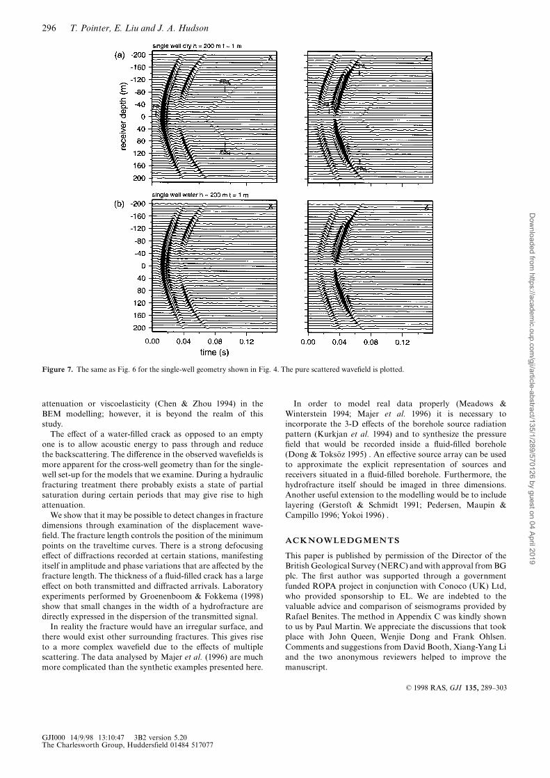
to those used for Fig. 6 except that the source and receivers arenow placed in a single-well geometry (Fig. 4). Only the purescattered ¢eld is shown. It is now possible to see the e¡ect of thepresence of a hydrofracture on the backscattered energy. There£ected (PP) and converted (PS) phases are easy to observe inaddition to the crack tip di¡ractions. As expected the re£ectedand di¡racted amplitudes are larger in the case of a cavityas some energy can travel through the £uid-¢lled fracture.However, the di¡erence in wave¢elds caused by the di¡erentin¢ll does not manifest itself so clearly as in the case of thecross-well geometry.

Figure 5. Ray-theoretical traveltimes (with respect to the centre of the incident pulse) for di¡racted, re£ected and transmitted waves (dashed). Thelabels are explained in Fig. 4. The traveltimes according to the models used to generate the seismograms in Figs 6, 8(a) and 8(c) (the change intraveltime due to the reduced crack opening is negligible) are shown in (a). The times in (b) correspond to the single-well geometry needed to produceFig. 7. The graph in (c) corresponds to Fig. 8(b)


ß 1998 RAS, GJI 135, 289^303


ownloaded from



Fracture length

A cross-well shot gather is shown in Fig. 8(b) for a water-¢lledfracture whose length is reduced to 100 m; it can be comparedwith Fig. 8(a), which is identical to Fig. 6(b). The arrival timesof the crack-tip di¡ractions are dramatically di¡erent. Thevertical extent of the fracture is still apparent from the PSdphases. There is much less transmitted energy in the form ofPPS owing to the reduced size of the fracture (clearly seen onthe z-component). The amplitude and phase of all the arrivalsare clearly a¡ected by the fracture length.

Fracture opening

A similar shot gather is shown in Fig. 8(c) for a water-¢lledcrack whose length remains at 200 m and crack openingis reduced to 0.1 m. The change in thickness allows moreenergy to pass through as PPP and PPS because lessenergy is attenuated through internal multiples. The crack-tipdi¡ractions are larger because more refracted energy canre-emerge at the crack ends. The same change in crack openingfor a dry crack has no visible e¡ect on the wave¢eld as there isno transmitted energy and the dominant wavelength is muchlarger than the crack width, although the results are not shownhere.

5 DISCUSSION

We have demonstrated that the BEM could be a useful tool foranalysing the scattering of seismic waves caused by hydraulicfractures. Our implementations for cavities and elasticinclusions is the same as those of Sanchez-Sesma & Campillo(1991) and Sanchez-Sesma & Luzon (1995), respectively,and similar to that of Coutant (1989) for the case of £uid-¢lled scatterers, except that we use the full-space £uidGreen's function. We have explained, in detail, the evaluationof the improper boundary integrals. From a comparison withanalytical solutions we have proved that our code produceshighly accurate results, although this may degenerate in theproximity of the crack corners.The synthetic experiments undertaken demonstrate how

P and S waves di¡racted at crack tips can be used to deter-mine the vertical extent of the fracture; this has beenachieved from the analysis of real data (Liu et al. 1997) . Theconverted PSd di¡ractions have a much stronger amplitudethan the PPd events, which suggests they could be a betterindicator of fracture length, with the potential to resolvesmaller-wavelength features. Energy that converts to inter-face waves at the fracture and is subsequently di¡ractedfrom the tips may be observable in real data if a suitable gain isapplied. It is straightforward to include frequency-independent

Figure 6. BEM synthetic horizontal- (x) and vertical- (z) component seismograms for the cross-well geometry depicted in Fig. 4. The total wave¢eldis plotted. The fracture length is 200 m and the fracture opening is 1 m. The traces shown in (a) and (b) correspond to a dry and a water-¢lled fracture,respectively. The energy marked with the label A occurs due to defocusing at the crack tips. The arrival labelled B is a P wave that arrives at the crackcentre, travels along the crack surface as a Stoneley wave and is di¡racted at both tips as a P wave.


ß 1998 RAS,GJI 135, 289^303


ownloaded from



attenuation or viscoelasticity (Chen & Zhou 1994) in theBEM modelling; however, it is beyond the realm of thisstudy.The e¡ect of a water-¢lled crack as opposed to an empty

one is to allow acoustic energy to pass through and reducethe backscattering. The di¡erence in the observed wave¢elds ismore apparent for the cross-well geometry than for the single-well set-up for the models that we examine. During a hydraulicfracturing treatment there probably exists a state of partialsaturation during certain periods that may give rise to highattenuation.We show that it may be possible to detect changes in fracture

dimensions through examination of the displacement wave-¢eld. The fracture length controls the position of the minimumpoints on the traveltime curves. There is a strong defocusinge¡ect of di¡ractions recorded at certain stations, manifestingitself in amplitude and phase variations that are a¡ected by thefracture length. The thickness of a £uid-¢lled crack has a largee¡ect on both transmitted and di¡racted arrivals. Laboratoryexperiments performed by Groenenboom & Fokkema (1998)show that small changes in the width of a hydrofracture aredirectly expressed in the dispersion of the transmitted signal.In reality the fracture would have an irregular surface, and

there would exist other surrounding fractures. This gives riseto a more complex wave¢eld due to the e¡ects of multiplescattering. The data analysed by Majer et al. (1996) are muchmore complicated than the synthetic examples presented here.

In order to model real data properly (Meadows &Winterstein 1994; Majer et al. 1996) it is necessary toincorporate the 3-D e¡ects of the borehole source radiationpattern (Kurkjan et al. 1994) and to synthesize the pressure¢eld that would be recorded inside a £uid-¢lled borehole(Dong & ToksÎz 1995) . An e¡ective source array can be usedto approximate the explicit representation of sources andreceivers situated in a £uid-¢lled borehole. Furthermore, thehydrofracture itself should be imaged in three dimensions.Another useful extension to the modelling would be to includelayering (Gerstoft & Schmidt 1991; Pedersen, Maupin &Campillo 1996; Yokoi 1996) .

ACKNOWLEDGMENTS

This paper is published by permission of the Director of theBritish Geological Survey (NERC) and with approval from BGplc. The ¢rst author was supported through a governmentfunded ROPA project in conjunction with Conoco (UK) Ltd,who provided sponsorship to EL. We are indebted to thevaluable advice and comparison of seismograms provided byRafael Benites. The method in Appendix C was kindly shownto us by Paul Martin. We appreciate the discussions that tookplace with John Queen, Wenjie Dong and Frank Ohlsen.Comments and suggestions from David Booth, Xiang-Yang Liand the two anonymous reviewers helped to improve themanuscript.

Figure 7. The same as Fig. 6 for the single-well geometry shown in Fig. 4. The pure scattered wave¢eld is plotted.


ß 1998 RAS, GJI 135, 289^303


ownloaded from



REFERENCES

Aki, K. & Richards, P., 1980, Quantitative Seismology: Theory andMethods,W.H. Freeman, New York.

Banerjee, P.K. & Butterfeld, R., 1981. Boundary Element Methods inEngineerng Science, McGraw-Hill, London.

Benites, R., Aki, K. & Yomogida, K., 1992. Multiple scattering of SHwaves in 2-D media with many cavities, Pure appl. Geophys., 138,353^390.

Bonnet, M., 1989. Regular boundary integral equations for three-dimensional ¢nite or in¢nite bodies with and without curved cracksin elastodynamics, Boundary Element Techniques: Applications inEngineering,ComputationalMechanicsPublications,Southampton.

Bouchon, M., 1987. Di¡raction of elastic waves by cracks or cavitiesusing the discrete wavenumber method, J. acoust. Soc. Am., 81,1671^1676.

Chapman, C.H. & Drummond, R., 1982. Body-wave seismograms ininhomogeneous media using Maslov asymptotic theory, Bull. seism.Soc. Am., 72, 277^317.

Chen, G. & Zhou, H., 1994. Boundary element modelling of non-dispersive and dispersive waves, Geophysics, 59, 113^118.

Coutant, O., 1989. Numerical study of the di¡raction of elastic wavesby £uid-¢lled cracks, J. geophys. Res., 94, 17 805^17 818.

Dom|nguez, J. & Abascal, R., 1984. On fundamental solutions forthe boundary integral equations method in static and dynamicelasticity, Eng. Analysis, 1, 128^134.

Figure 8. The synthetic seismograms in (a) are the same as in Fig. 6(b). The traces in (b) and (c) are also calculated using a cross-well geometry and awater-¢lled fracture. The fracture length in (b) is reduced to 100 m and the thickness remains at 1 m, whereas in (c) the fracture opening decreasesto 0.1 m and the length is kept at 200 m. In each case the total wave¢eld is displayed.


ß 1998 RAS,GJI 135, 289^303


ownloaded from



Dong, W., 1993. Elastic wave radiation from borehole seismic sourcesin anisotropic media, PhD thesis, MIT, Cambridge, USA.

Dong, W. & Tokso« z, M.N., 1995. Borehole seismic-source radiationin layered isotropic and anisotropic media: real data analysis,Geophysics, 60, 748^757.

Dong, W., Bouchon, M. & Tokso« z, M.N., 1995. Borehole seismic-source radiation in layered isotropic and anisotropic media:boundary element modelling, Geophysics, 60, 735^747.

Fehler, M. & Aki, K., 1978. Numerical study of di¡raction of planeelastic waves by a ¢nite crack with application to location of amagma lens, Bull. seism. Soc. Am., 68, 573^598.

Gerstoft, P. & Schmidt, H., 1991. A boundary element approachto ocean seismoacoustic facet reverberation, J. acoust. Soc. Am., 89,1629^1642.

Gra¤, D., 1946. Sul teorema di reciprocita nella dinamica dei corpoelastici, Memorie della Accademia delle Scienze, 4, 103.

Groenenboom, J. & Fokkema, J.T., 1998. Monitoring the width ofhydraulic fractures with acoustic waves, Geophysics, 63, 139^148.

Kawase, H., 1988. Time-domain response of a semi-circular canyonfor incident SV, P, and Rayleigh waves calculated by the discretewavenumber boundary element method, Bull. seism. Soc. Am., 78,1415^1437.

Krishnasamy, G., Rizzo, F.J. & Liu, Y., 1994. Boundary integralequations for thin bodies, Int. J. Num. Meth. Eng., 37, 107^121.

Kurkjan, A.L., Coates, R.T., White, J.E. & Schmidt, H., 1994. Finite-di¡erence and frequency-wavenumber modelling of seismic mono-pole sources and receivers in £uid-¢lled boreholes, Geophysics, 59,1053^1064.

Liu, E., Hudson, J.A., Crampin, S., Rizer, W.D. & Queen, J.H., 1995.Seismic properties of a general fracture, in Proc. 2nd Int. Conferenceon the Mechanics of Jointed and Faulted Rock, pp. 673^678, ed.Rossmanith, Balkema, Rotterdam.

Liu, E., Crampin, S. &Hudson, J.A., 1997. Di¡raction of seismic wavesby cracks with application to hydraulic fracturing, Geophysics, 62,253^265.

Lysmer, J. & Drake, L.A., 1972. A ¢nite element method for seismo-logy, Methods of Computational Physics, Vol. 11, Academic Press,New York.

Majer, E.L. et al., 1996. Utilising crosswell, single well and pressuretransient tests for characterising fractured gas reservoirs, LeadingEdge, 15, 951^956.

Mal, A.K., 1970. Interaction of elastic waves with a Gri¤th crack, Int.J. Eng. Sci., 8, 763^776.

Meadows, M.A. & Winterstein, D.F., 1994. Seismic detection of ahydraulic fracture from shear-wave VSP data at Lost Hills Field,California, Geophysics, 57, 11^26.

Neuberg, J. & Pointer, T., 1995. Modelling seismic re£ections fromD@ using the Kirchho¡ method, Phys. Earth planet. Inter., 90,273^281.

Pao, Y.H. & Mow, C.C., 1973. The Di¡raction of Elastic Waves andDynamic Stress Concentrations, Crane & Russak, New York.

Pedersen, H., Maupin, V. & Campillo, M., 1996. Wave di¡raction inmultilayered media with the Indirect Boundary Element Method:application to 3-D di¡raction of long-period surface waves by 2-Dlithospheric structures, Geophys. J. Int., 125, 545^558.

Press, W.H., Teukolsky, S.A., Vetterling, W.T. & Flannery, B.P., 1992.Numerical Recipes in Fortran: the Art of Scienti¢c Computing,2nd edn, Cambridge University Press, Cambridge.

Ricker, N.H., 1977. Transient Waves in Visco-elastic Media, Elsevier,Amsterdam.

Ryshik, I.M. & Gradstein, I.S., 1963. Tables of Series, Products andIntegrals,VEB Deutscher Verlag der Wissenschaften, Berlin.

Sanchez-Sesma, F.J. & Campillo, M., 1991. Di¡ractions of P, SV,and Rayleigh waves by topographic features: a boundary integralformulation, Bull. seism. Soc. Am., 81, 2234^2253.

Sanchez-Sesma, F.J. & Luzon, F., 1995. Seismic response of three-dimensional alluvial valleys for incident P, S, and Rayleigh waves,Bull. seism. Soc. Am., 85, 269^284.

Tadeu, A.J.B., Kausel, E. & Vrettos, C., 1996. Scattering of waves bysubterranean structures via the boundary element method, SoilDyn. Earthq. Eng., 15, 387^397.

Vinegar, H.J. et al., 1992. Active and passive imaging of hydraulicfractures, Leading Edge, 11, 15^22.

Wang, C.-Y., Achenbach, J.D. & Hirose, S., 1996. Two-dimensionaltime domain BEM for scattering of elastic waves in solids of generalanisotropy, Int. J. Solids Structures, 33, 3843^3864.

Wu, R.S., 1994. Wide-angle elastic wave one-way propagation inheterogeneous media and an elastic wave complex-screen method,J. geophys. Res., 99, 751^766.

Wu, R.S. & Aki, K., 1985. Scattering characteristics of elastic waves byan elastic heterogeneity, Geophysics, 50, 582^589.

Yokoi, T., 1996. An indirect boundary element method based onrecursive matrix operation to compute waves in irregularly strati¢edmedia with in¢nitely extended interfaces, J. Phys. Earth, 44, 39^60.

Yokoi, T. & Sanchez-Sesma, F.J., 1998. A hybrid calculation tech-nique of the indirect boundary element method and the analyticalsolutions for three-dimensional problems of topography, Geophys.J. Int., 133, 121^139.

APPENDIX A: 2-D BOUNDARY ELEMENTMETHOD THEORY

Elastic medium

The reciprocal theorem relates two di¡erent boundary valueproblems on the same region with the same boundary. Itstates that the work done by one set of forces f and boundarytractions t on the set of displacements u* in the other systemis equal to the work done by the second set of forcesf* and tractions t* on the ¢rst displacements u. We deal withthe steady-state elastodynamic problem and assume that thephysical components in the representation are harmonic intime with an angular frequency u. The reciprocal theorem forthe 2-D elastodynamic case (Gra¤ 1946) may be expressed as�Sti(x, u)u1i(x, u) dsz

� �D

fi(x, u)u1i(x, u) dA

~

�St1i(x, u)ui(x, u) dsz

� �D

f 1i(x, u)ui(x, u) dA , (A1)

where S is the boundary to the region D. The result is a directconsequence of the symmetry in the elastic tensor, {cijkl~cklij},which arises from the existence of a strain-energy function.A representation for the displacement ¢eld u can be obtained

by replacing the other displacement ¢eld u* with the Green'sfunction Gij , the fundamental singular solution to the elasticwave equation (Appendix B), and correspondingly the body-force term f* with a delta impulse (Aki & Richards 1980) . Theresulting Somigliana representation theorem expresses thedisplacement u(r) at a point j as an integral of the displace-ments and tractions over the boundary S (with respect to x),together with an integral over body forces within S (withrespect to y):

aIu(r)j (j, u)

~

�S[GI

ij(x, j, u)tIi (x, u){uIi (x, u)cIipkl nª pGIkj,l(x, j, u)] dsx

z

� �DI

f Ii (y, u)GIij(y, j, u) dAy ,

aI~1 j in DI ,

0 j not in DI ,

((A2)


ß 1998 RAS, GJI 135, 289^303


ownloaded from



where GIij is the Green's function for the region DI interior to

S andGIkj,l(x, j)~LGI

kj(x, j)/Lxl ; fcIijpqg are the sti¡nesses inDI,and uI and tI are the limits of u(r) and t(r) as S is approachedfrom the interior. The outward normal to S is given by nª .To evaluate the right-hand side of eq. (A2) when j is situatedon the boundary, we consider the limit as j approaches theboundary S (Appendix C), which is assumed to be smooth,from inside DI. We can rewrite eq. (A2) as

aIu(r)j (j)~P�S[GI

ij(x, j)tIi (x){uIi (x)TIij(x, j)] dsx

z

� �DI

f Ii (y)GIij(y, j) dAy , (A3)

aI~

1 j in DI ,

0 j not in DI ;

0:5 j on S ,

8>><>>:where we have substituted the expression for the tractionGreen's function Tij(x, j)~cipkl nª p(x)Gkj,l(x, j). P denotesthe Cauchy Principal Value (Appendix C). Eq. (A3) is therepresentation used in the direct BEM. The boundary con-ditions on S are applied to determine the unknown boundaryvalues uI(x) and tI(x). It is then possible to use eq. (A3) againto calculate the displacements at any point j in DI (Kawase1988).We now replace the material in the regionDE, exterior toDI,

by one that has the same sti¡nesses and density as in DI, andin which there are no sources. In doing so we shift the in£uenceof the material in DE to the boundary S. By taking the limitas j approaches S from outside DI we can write a similarrepresentation for the displacement in the exterior region:

aEu¬ j(j)~{P�S[GI

ij(x, j) t¬ i(x){u¬ i(x)T Iij(x, j)] dsx , (A4)

aE~

0 j in DI ,

1 j not in DI ;

0:5 j on S .

8>><>>:The body-force integral is dropped as it is zero. There is achange in sign in the integral over S since the sense of theoutward normal to S is reversed. We use the same Green'sfunction, GI, as for the interior region since the material is thesame. This must therefore satisfy the radiation conditions foroutgoing waves. The limiting values u¬ and t¬ of the displace-ments and tractions are unspeci¢ed as yet. We can sum eqs(A3) and (A4) to obtain a representation for the displacementat any point j on S:

12[uIj (j)zu¬ j(j)]

~P�S{GI

ij(x, j)[tIi (x){ t¬ i(x)]{T Iij(x, j)[uIi (x){u¬ i(x)]} dsx

z

� �DI

f Ii (y)GIij(y, j) dAy . (A5)

We specify the solution outside DI to be that which establisheson S exactly the same boundary displacements as those in theinitial interior-region problem [so that u¬ (j)~uI(j), j [S]. Itfollows that, in general, tI(j)=tE(j). We now substitute uI(j)

for u¬ (j) in eq. (A5) to obtain

uIj (j)~�SGI

ij(x, j)[tIi (x){ t¬ i(x)] dsxz� �

DIf Ii (y)G

Iij(y, j) dAy .

(A6)

With the notation wI(x)~tI(x){ t¬ (x), we can rewrite eq. (A6)as

uIj (j)~�SGI

ij(x, j)�Ii (x) dsxz� �

DIf Ii (y)G

Iij(x, j) dAy , (A7)

which shows that wI(x) dsx represents a ¢ctitious line-forcedistribution. Due to symmetry in the displacement Green'sfunction [Gij(x, j)~Gji(j, x)] we can restate eq. (A7) as:

uIi (x)~�SGI

ij(x, j)�Ij (j) dsjz

� �DI

f Ij (j)GIij(x, j) dAj . (A8)

This integral representation (without the last term) is knownas a single-layer potential and is classi¢ed as indirect becausethe scattered wave¢eld is given in terms of unknown sourcestrengths located on the boundary. It is a mathematicalexpression of Huygen's principle, whereby every point on theboundary can be considered as a source of secondary wavelets.We have shown above the formal equivalence of the direct(eq. A3) and indirect (eq. A8) BEMs. Note that we couldequally have chosen the solution outside S as that whichestablishes on S that tE(j)~tI(j).By application of Hooke's law to both sides of eq. (A8),

an indirect representation of the interior tractions can bestated:

tIi (x)~12�Ii (x)zP

�ST Iij(x, j)�Ij (j) dsj

zcipkl nª pL

LxlP� �

DIf Ij (j)G

Ikj(x, j) dAj , (A9)

where the ¢rst term on the right-hand side is a `free term' due tothe singularity when x coincides with j on S, which is assumedto be smooth (Appendix C). The second term must again betreated as a Cauchy Principal Value.The combination of eqs (A3) and (A4) also gives the

displacement at any point x within DI:

u(r)i (x)~�SGI

ij(x, j)�Ij (j) dsjz

� �DI

f Ij (j)GIij(x, j)dAj . (A10)

In a similar way, the di¡racted (outgoing) displacementsu(d) in the exterior region DE can be represented in terms ofunknown source functions wE:

u(d)i (x)~�SGE

ij (x, j)�Ej (j) dsjz

� �DE

f Ej (j)GEij (x, j) dAj ,

(A11)

where GEij is the appropriate Green's function for the material

in DE. The limiting values u¬ E and t¬ E of the displacements u(r)

and corresponding tractions t(r) on S are given by

uEi (x)~�SGE

ij (x, j)�Ej (j) dsjz

� �DE

f Ej (j)GEij (x, j) dAj ,

tEi (x)~{12�Ei (x)zP

�STEij (x, j)�Ej (j) dsj (A12)

zcikpqnª kL

Lxq

� �DE

f Ej (j)GEpj(x, j) dAj .


ß 1998 RAS,GJI 135, 289^303


ownloaded from



The unknown functions wE and wI are determined by matchingthe displacements and tractions on S due to, on the onehand, a combination of the interior refracted ¢eld u(r) and theexterior di¡racted ¢eld u(d), and on the other hand, the incidentradiation u(i):

uEj (x){uIj (x)~{u(i)j (x) ,

tEj (x){tIj (x)~{t(i)j (x) , x [S .(A13)

Fluid medium

A similar procedure can be used to derive direct and indirectrepresentations for wave motion in a £uid medium (Dong1993) . The direct representation for the interior displacementpotential t at a point j is, in the absence of sources,

aIt(r)(j)~P�Snª i(x) GI(x, j)

LtI(x)Lxj

{tI(x)LGI(x, j)

Lxj

� �idsx ,

(A14)

aI~

1 j in DI ,

0 j not in DI ;

0:5 j on S ,

8>><>>:where nª (x) is the outward-pointing unit normal at x and GI

is the scalar potential Green's function for a £uid medium(Appendix B). The corresponding indirect expression is

t(r)(x)~�SGI(x, j)�I(j) dsj , (A15)

where �I(j) is a distribution of ¢ctitious sources. The indirectintegral for the normal displacement u~=t . nª at a point x onthe boundary S is

uI(x)~12�I(j)zP

�sT I(x, j)�I(j) dsj , (A16)

in which T I is the normal displacement Green's function for a£uid medium:

T I(x, j)~nª i(x)LGI(x, j)

Lxi. (A17)

The pressure in the £uid is given by p(r)~ou2t(r), where o is the£uid density, so the normal traction at the boundary is

tI(x)~{pI(x)

~{ou2�SGI(x, j)�I(j) dsj , x [S .

(A18)

If the exterior region is solid, the conditions determining �I

and wE are

uEj (x)nª j(x){uI(x)~{u(i)j (x)nª j(x) ,

tEj (x)nª j(x){tI(x)~{t(i)j (x)nª j(x) ,

tEj (x)mª j(x)~{t(i)j (x)mª j(x) ,

(A19)

where mª is a unit tangent to S at x.

APPENDIX B: GREEN'S FUNCTIONS FOR2-D ISOTROPIC MEDIA

Elastic medium

The Green's function for SH motion is given by

G(x, j)~14ki

H(2)0 (kbr) , r~jx{jj , (B1)

where kb~u/b, and b and k are respectively the S-wave speedand the modulus of rigidity in the material. This represents thedisplacement at x due to an anti-plane unit force at j.For steady-state P^SV motion, the Green's function

describes the displacement at x in the ith direction as a resultof the application of an in-plane unit force in the jth directionat j:

Gij(x, j)~i4k

dijH(2)0 (kbr){

1kbr

LrLxi

LrLxj

�

| H(2)1 (kbr){

baH(2)

1 (kar)� ��

{i4k

LrLxi

LrLxj

H(2)0 (kbr){

b2

a2H(2)

0 (kar)

" #( ),

r~jx{jj , (B2)

where ka~u/a and a is the P-wave speed.

Fluid medium

The displacement potential Green's function in a £uid takes asimilar form to the displacement for SH in an elastic medium:

G(x, j)~14i

H (2)0 (kf r) , (B3)

where kf , the wavenumber inside the £uid, is given by u/c,and c is the wave speed in the £uid.The Green's functions given above can be found in

Dom|nguez & Abascal (1984).

APPENDIX C: EVALUATION OF THEBOUNDARY INTEGRALS

Expressions such as eq. (A2) for the displacement u(r)(j) withinthe region DI, that involve integrals like�SGij(x, j)(i(x) dsx

and�STij(x, j)ti(x) dsx (C1)

are not simple to evaluate in the limit as j approaches theboundary S since both Gij and Tij are singular at j~x. Weassume that the boundary is smooth and that C and yrepresent continuous functions.The Green's function Gij in plane strain (P^SV motion)

is given by eq. (B2) and is a function of kar and kbr, whereka~u/a, kb~u/b and r~jx{jj. The limit r?0 is, therefore,the same as the limit kar?0 and also u?0; that is, theasymptotic behaviour for small r is the same as that for low


ß 1998 RAS, GJI 135, 289^303


ownloaded from



frequency, or the static limit. The 2-D static Green's functionGs

ij(x, j) is given by Banerjee & Butter¢eld (1981) as

Gsij(x, j)~

{18nk(1{l)

{(3{4l) dij log r{rª i rª j}zAij , (C2)

where l is Poisson's ratio, rª i~(xi{mi)/r and Aij is a constanttensor. There is therefore a logarithmic singularity in Gij atx~j, but this is integrable. The ¢rst of the integrals in eq. (C1)may therefore be evaluated in the limit as j?xS[S by simplysetting j~xS in the integrand and evaluating the improperintegral.The second of the integrals in (C1) involves Tij(x, j), given by

Tij(x, j)~cipkl nª p(x)L

LxlGkj(x, j) , (C3)

where nª (x) is the outward normal to the boundary S. The staticequivalent of this is (Banerjee & Butter¢eld 1981)

T sij(x, j)~

{14nr(1{l)

{(1{2l)(nª j rª i{nª i rª j)

z[(1{2l)dijz2rª i rª j ]rª knª k} , (C4)

and this has a (1/r) singularity that is not integrable whenj~xS[S. We therefore need to look carefully at the details ofthe limit as j?xS, where xS is any point of S.The derivation of the ¢nal result given by Banerjee &

Butter¢eld (1981) is given only for the acoustic (scalar) caseand is, in any case, not valid in all circumstances.Consider the point j within the region DI as it approaches a

point xS on the boundary S of DI (see Fig. C1). We split thecurve S into two parts, namely S�, a section of curve centred onxS and of length � on either side, and S'~S{S�. The main taskis to evaluate

limj?xS

�S�

Tij(x, j)ti(x) dsx . (C5)

To do this, we split the integral into two further parts:�S�

Tij(x, j)ti(x) dsx~ti(xS)�S�

Tij(x, j) dsx

z

�S�

Tij(x, j)[ti(x){t(xS)] dsx . (C6)

If y is HÎlder continuous on S,

jti(x1){ti(x2)j¦Ljx1{x2ja (C7)

for any two points x1, x2 of S, where L and a are constants,with 0 < a¦1. On the assumption that this inequality holds,the second integral in eq. (C6) is integrable and bounded whenj~xS. It remains to evaluate the ¢rst of the integrals in (C6).

We have assumed that S is smooth and so wemay replace thecurve S� by a section of straight line, tangent to S� at xS (seeFig. C2) with error of the order of �:�S�

Tij(x, j) dsx~��

{�

Tij(x, j) dxzO(�) , (C8)

where we have set up axes oriented such that xS lies atthe origin, the x-axis lies along the tangent [so thatx~(x, 0), {�¦x¦�] and the y-axis points into DI so thatj~(0, g), nª (x)~(0, {1).Since jx{jj is arbitrarily small in this integral, we use the

static form for Tij. Substituting for x, j and nª in eq. (C4) weobtain

T11(x, j)~{1

4nr(1{l)gr

1{2lz2x2

r2

� �,

T12(x, j)~{1

4nr(1{l){(1{2l)

xr

{2g2xr3

� �,

T21(x, j)~{1

4nr(1{l)(1{2l)

xr{

2g2xr3

�g ,

T22(x, j)~{1

4nr(1{l)gr

1{2lz2g2

r2

� �,

(C9)

where r~(x2zg2)1=2. In the integration over x, odd powers of xgive zero contribution, so that the integrals of T12 and T21 areboth zero.The remaining integrals are��

{�

T11(x, j) dx~{g

4n(1{l)

��{�

1{2lx2zg2

z2x2

(x2zg2)2

� �dx

~{1

4n(1{l)4(1{l) tan{1 �/g{

2�g(�2zg2)

� �,��

{�

T22(x, j) dx~{g

4n(1{l)

��

{�

1{2lx2zg2

z2g2

(x2zg2)2

� �dx

~{1

4n(1{l)4(1{l) tan{1 �/gz

2�g(�2zg2)

� �.

(C10)

If we now let j?xS (g?0), we have�S�

Tij(x, j) dsx~{12

dijzO(�) . (C11)

Figure C1. The boundary S is divided into two parts by taking out asection S� of length 2�, with the boundary point xS in the middle.

Figure C2. The section of boundary S� is replaced by an interval[{�, �] on the tangent at the point xS.


ß 1998 RAS,GJI 135, 289^303


ownloaded from



Finally, we allow � to tend to zero. The integral over S' becomesa Cauchy Principal Value and the second integral on the rightof eq. (C6) tends to zero. Thus

limj?xS, j[DI

�STij(x, j)ti(x) dsx

~P�STij(x, xS)ti(x) dsx{

12tj(x

S) . (C12)

If the point j lies outside DI, we may repeat the derivation,changing the sign of g in eq. (C9). This leads to the same resultexcept that the sign of the `free term' is changed:

limj?xS, j=[DI

�STij(x, j)ti(x) dsx

~P�STij(x, xS)ti(x) dsxz

12tj(x

S) . (C13)

These results justify the step from eq. (A2) to eq. (A3).The derivation of eq. (A9) from (A8) follows a slightly

di¡erent path. Eq. (A8) shows the displacement within DI

represented in terms of a single-layer potential w; that is, withthe body force f set to zero:

ui(x)~�SGij(x,j)�j(j)dsj,, x[DI : �C14�

The corresponding stress ¢eld is

pij(x)~�ScijpqGpk,q(x, j)�k(j) dsj , x [DI . (C15)

We need to evaluate the displacements and tractions on S.As before, the singularity in Gij at x~j is integrable and wemay simply put x~xS in eq. (C13). To ¢nd the tractions, weneed to take the limit as x?xS:

ti(xS)~ limx?xS

�Scijpqnª j(xS)Gpk,q(x, j)�k(j) dsj . (C16)

This is similar to taking the limit as j?xS of the secondintegral in (C1) except that nª (x) is replaced by nª (xS) and theintegration is over j instead of x. We may in fact write

ti(xS)~ limx?xS

�SFij(x, j)�j(j) dsj , (C17)

where

Fij(x, j)~cipkl nª p(xS)L

LxlGkj(x, j) . (C18)

We proceed as before to evaluate the integral in (C17) bydividing the range of integration into a part over S� and a partover S'~S{S�. The integral over S' will become a CauchyPrincipal Value when �?0; the integral over S� is partitioned asin eq. (C6):�S�

Fij(x, j)�j(j) dsm~�j(xS)�S�

Fij(x, j) dsj

z

�S�

Fij(x, j)[�j(j){�j(xS)] dsj . (C19)

The second integral is bounded as x?xS and tends to zero as�?0. It remains, therefore, to evaluate the ¢rst integral andtake the limit as x?xS. This proceeds exactly as for the integralover Tij in (C8) except that x and j have been interchanged.Since Tij (and therefore Fij) is an odd function of rª~(x{j)/r,

the result is as before but with the opposite sign:�S�

Fij(x, j) dsj~12

dijzO(�) . (C20)

We now let �?0 to obtain

ti(xS)~P�sTij(xS, j)�j(j) dsjz

12�i(xS) , (C21)

which leads to eq. (A9).The derivation of eq. (A12) proceeds in exactly the same way

except that the limit is approached from outside DI and so thesign of the free term is changed.The corresponding expressions for the anti-plane-strain

(SH) problem involve integrals such as�sG(x, j)((x) dsx

and�sT (x, j)t(x) dsx , (C22)

where the Green's function is now (eq. B1)

G(x, j)~14ki

H(2)0 (kbr) (C23)

and

T (x, j)~knª j(x)L

LxjG(x, j)~

{kbnª j(x)rª j4i

H(2)1 (kbr) ; (C24�

nª (x) is once again the unit outward normal on S.The leading terms for the Hankel functions of small

argument are (Ryshik & Gradstein 1963)

H(2)0 (z)~

{2in

log zzO(1) ,

H(2)1 (z)~

2inz

zO(1) .

(C25)

It follows, as for the plane-strain case, that the ¢rst integral in(C22) may be evaluated directly for j~xS[S, whereas we needto take the limit j?xS to evaluate the second.We proceed, as before, to write�

ST (x, j)t(x) dsx~

�S0

T (x, j)t(x) dsxz�S�

T (x, j)t(x) dsx .

(C26)

The ¢rst integral takes the Cauchy Principal Value when x~xS

and �?0. The second integral becomes�S�

T (x, j)t(x) dsx~t(xS)�S�

T (x, j) dsx

z

�S�

T (x, j)[t(x){t(xS)] dsx : (C27)

The second integral here is bounded as x?xS (assumingHÎlder continuity for t) and tends to zero as �?0. The ¢rstbecomes�S�

T (x, j) dsx~��

{�

T (x, j) dxzO(�) (C28)

by the replacement of S� by a section of the tangent at xS

(see Fig. C2).


ß 1998 RAS, GJI 135, 289^303


ownloaded from



We choose axes so that xS~(0, 0), j~(0, g), x~(x, 0) andnª ~(0, {1); thus,

T (x, j)~{g2nr2

zO(1) , (C29)

where r2~x2zg2. Substituting back into (C28) and performingthe integration, we obtain�S�

T (x, j) dsx~{1ntan{1 (�/g)zO(�) . (C30)

Finally we take the limits g?0 and then �?0 to obtain

limj?xS

�ST (x, j)t(x) dsx~P

�ST (xS, j)t(x) dsx{

12t(xS) .

(C31)

This establishes the formula in anti-plane strain for points jon S.

Exactly the same procedure can be followed to establisheqs (A9) and (A12) and the signs of the free terms foranti-plane strain.For a £uid medium, the expressions that need to be

evaluated are the same as in eq. (C22) but with (eq. B3)

G(x, j)~14i

H (2)0 (kf r) (C32)

and

T (x, j)~nª j(x)L

LxjG(x, j)~

{kf nª j(x)rª j4i

H(2)1 (kf r) , (C33)

where kf is the wavenumber in the £uid. Thus T is exactly thesame as for anti-plane-strain (SH) motion in a solid and thelimit of the integral as x?xS[S is the same. This establishes(A14) and (A16).


ß 1998 RAS,GJI 135, 289^303


ownloaded from



numerical modelling of seismic waves scattered by hydrofractures

Documents