numerical modelling of sound transmission in lightweight ... · numerical modelling of sound...

Universitat Politecnica de Catalunya

Programa de Doctorat d’Enginyeria Civil

Laboratori de Calcul Numeric

Numerical modelling of sound

transmission in lightweight structures

by Jordi Poblet-Puig

Doctoral Thesis

Advisor: Antonio Rodrıguez-Ferran

Barcelona, January 2008

Abstract

Numerical modelling of soundtransmission in lightweight structures

Jordi Poblet-Puig

The thesis deals with the numerical modelling of sound transmission. All the

analyses are done in the frequency domain and assuming that the structures are

linear and elastic. Linear acoustics is considered for the fluid domains. Thus, the

fluid-structure interaction problems analysed here are governed by the vibroacoustic

equations. The models are applied to the field of building acoustics, with especial

interest on lightweight structures.

A set of one-dimensional models for single and layered partitions considering finite

acoustic domains is developed. Preliminary parametric analyses are done, considering

aspects like the acoustic absorption, the structural damping, the separation between

layers, the quality of absorbing material, or the influence of the eigenfrequencies of

the problem in the isolation capacity. The analytical solution of these situations is

available and it is used to test two and three-dimensional models.

Numerical-based models for vibroacoustic problems lead to large system of lin-

ear equations. This is an important drawback for mid and high-frequencies where

the computational costs become unaffordable. The block Gauss-Seidel algorithm has

been applied for sound transmission problems. Its performance has been analysed

by means of analytical expressions of the spectral radius obtained in one-dimensional

situations. Moreover, a selective coupling strategy is developed in order to efficiently

iii

solve problems where some acoustic domains are strongly coupled (i.e. double walls).

In building acoustics, the acoustic domains are often cuboid-shaped rooms. Ana-

lytical expressions of the eigenfunctions are well known and can be used in order to

obtain the pressure field by means of a modal analysis. A model that combines this

with a more general finite element (FEM) description of the structure is presented.

This mixed approach is more efficient (time and memory requirements) than a FEM-

FEM model. The most relevant aspects of the modal-FEM approach are analysed:

computational costs, modelling of acoustic absorption, selection of the modal basis.

The model is used in order to predict the isolation capacity of single and double

walls. Heavy and lightweight structures are considered. The influence on the sound

reduction index of parameters related with the wall environment like the room size,

the position of the source, the correction due to acoustic absorption is shown. Wall

properties such as its size, the damping or the boundary conditions are also considered,

as well as more specific aspects related with double walls (cavity thickness, quality of

the absorbing material).

The effect of flanking transmissions on the sound reduction index is also taken into

account. The vibration level difference and the sound transmission through several

junction types (L, T and X-shaped) are calculated. In the X-shaped junction case,

four rooms are analysed at the same time. The transmission between two of them is

only caused by flanking paths. The possibilities of numerical models are illustrated

with a case-study where the isolation capacities of a double wall with and without

an accurate acoustic design are compared. The existence of a vibration transmission

path between the floor and the leaves of the wall drastically reduces its performance.

The response of double walls depends on the type of mechanical connections be-

tween leaves. The attention is focused here on the case of lightweight steel studs. They

have been characterised by means of an equivalent spring. The value of the stiffness of

the spring is obtained by comparison of the vibration level difference between leaves

of a double wall obtained with two different models: i) considering the geometry of

the stud; ii) using springs instead of studs. Spectral structural finite elements are

used in order to increase the frequency range.

iv

These steel studs also modifie the radiation properties of unsymmetrical floors.

The different radiation efficiency between a planar face or a face with studs is cal-

culated by means of a numerical model using boundary elements. Differences are

significant. This is a clear example of how the details of the structure are important

in order to perform accurate predictions of sound isolation.

v

Acknowledgments

I would like to thank my advisor Antonio Rodrıguez-Ferran, for his dedication,

patience, and objective point of view. He has dedicated a lot of time and efforts in

order to improve the contents of the research and the quality of the final document.

This thesis has been done in an excellent research framework, the Laboratori de

Calcul Numeric (LaCaN). I am very grateful to Antonio Huerta for the extra effort

that suppose being at the head of this human group and giving me the opportunity to

join the team. I appreciate very much the support and friendship of all the colleagues

along these years. I would like to mention the help of Pedro Dıez in order to obtain the

grant and understand numerical errors, the numerous tricks revealed by the mestre

Xevi Roca, and the comprehension and scientific conversations with Nati Pastor.

It is thanks to the guideline provided by Alfredo Arnedo some years ago that I

started Ph.D. studies. He convinced me to enter into the research world.

I spent five months in the Centre Scientifique et Technique du Batiment (CSTB)

in Saint Martin d’Heres. This period has been very important in my personal and

academical education and decisive in the development of the thesis. The people that

I found there made the adaptation easy and the stage very pleasant. I would like to

thank Catherine Guigou for her sincere scientific opinions and for sharing her acoustic

knowledge and modelling results with me, Michel Villot for providing ideas, proposing

technological objectives and contributing with his experience in the field of acoustics

and vibration, and Philippe Jean for the very productive discussions on the numerical

modelling of vibroacoustic phenomena.

The development of this work has been simultaneous in time with the ‘High qual-

ity acoustic and vibration performance of lightweight steel constructions (ACOUSVI-

vii

BRA)’ project. The technological challenges and the empirical information provided

by the project have been important in order to enrich the thesis contents. I would

like to thank the partners for the nice discussions and experiences.

Many other people have helped me during this time with scientific discussions or

sending papers and references. Among others, Dr. Bouillard, Dr. Brunskog, col-

leagues and teachers of Computational Aspects of Structural Acoustics and Vibration

course at CISM and the members of the Laboratori d’Enginyeria Acustica i Mecanica

(LEAM, UPC).

I have been mainly using free software like Gmsh, PETSc, LAPACK, GSL, Open-

FEM or Code-Aster in a Linux environment during the thesis and the finite element

code CASTEM for a long time. I would also like to thank Free Field Technologies for

providing a free license for using ACTRAN and its user manual.

Thanks a lot to my family, my parents Conxa i Albert, my sister Mıriam, for

unconditional support, understanding and respect and to tiet Coque for being always

a technological reference. I appreciate very much the comprehension and opinions

from all of my friends, such as Alfredo and Giuseppe.

The financial support of the Generalitat de Catalunya i el Fons Social Europeu

(2003 FI 00652), the Research Fund for Coal and Steel, el Departament de Matematica

Aplicada III, Departament d’Infraestructura del Transport i del Territori and the Es-

cola Tecnica Superior d’Enginyers de Camins Canals i Ports is gratefully acknowl-

edged.

viii

Contents

Abstract iii

Acknowledgments vii

Contents xii

List of symbols xiii

1 Introduction 11.1 Different models for sound transmission problems . . . . . . . . . . . . 11.2 Lightweight structures and vibroacoustics . . . . . . . . . . . . . . . . . 41.3 Acoustic standards and regulations . . . . . . . . . . . . . . . . . . . . 51.4 Goals, scope and outline of the thesis . . . . . . . . . . . . . . . . . . . 81.5 Review of vibroacoustics equations . . . . . . . . . . . . . . . . . . . . 10

1.5.1 The acoustic problem . . . . . . . . . . . . . . . . . . . . . . . . 101.5.2 Acoustic problem types . . . . . . . . . . . . . . . . . . . . . . . 141.5.3 Analysis in the frequency-domain: the Helmholtz equation . . . 17

2 Review of numerical methods for vibroacoustics 232.1 Numerical methods for the low-frequency range . . . . . . . . . . . . . 24

2.1.1 The finite element method (FEM) . . . . . . . . . . . . . . . . . 242.1.2 The boundary element method (BEM) . . . . . . . . . . . . . . 262.1.3 Numerical techniques for the coupled problem . . . . . . . . . . 31

2.2 Numerical methods for the mid-frequency range . . . . . . . . . . . . . 362.2.1 Acoustic problems . . . . . . . . . . . . . . . . . . . . . . . . . 382.2.2 Structural dynamics . . . . . . . . . . . . . . . . . . . . . . . . 45

2.3 Concluding remarks . . . . . . . . . . . . . . . . . . . . . . . . . . . . . 49

3 One-dimensional model for vibroacoustics 513.1 Introduction . . . . . . . . . . . . . . . . . . . . . . . . . . . . . . . . . 513.2 One-dimensional model for undamped vibroacoustics . . . . . . . . . . 52

3.2.1 Problem statement . . . . . . . . . . . . . . . . . . . . . . . . . 52

ix

3.2.2 Analytical solution . . . . . . . . . . . . . . . . . . . . . . . . . 553.2.3 Application example . . . . . . . . . . . . . . . . . . . . . . . . 57

3.3 One-dimensional model for damped vibroacoustics . . . . . . . . . . . . 623.3.1 Problem statement . . . . . . . . . . . . . . . . . . . . . . . . . 623.3.2 Analytical solution . . . . . . . . . . . . . . . . . . . . . . . . . 633.3.3 Application examples . . . . . . . . . . . . . . . . . . . . . . . . 64

3.4 One-dimensional model of layered partitions . . . . . . . . . . . . . . . 673.4.1 Problem statement . . . . . . . . . . . . . . . . . . . . . . . . . 673.4.2 Analytical solution . . . . . . . . . . . . . . . . . . . . . . . . . 703.4.3 Application examples . . . . . . . . . . . . . . . . . . . . . . . . 71

3.5 Validation of finite element models . . . . . . . . . . . . . . . . . . . . 733.6 Concluding remarks . . . . . . . . . . . . . . . . . . . . . . . . . . . . . 75

4 The block Gauss-Seidel method in sound transmission problems 774.1 Introduction . . . . . . . . . . . . . . . . . . . . . . . . . . . . . . . . . 774.2 The block Gauss-Seidel algorithm . . . . . . . . . . . . . . . . . . . . . 784.3 Review of block iterative solvers in acoustics . . . . . . . . . . . . . . . 804.4 Influence of the degree of coupling . . . . . . . . . . . . . . . . . . . . . 814.5 Analysis of the block Gauss-Seidel method . . . . . . . . . . . . . . . . 83

4.5.1 The convergence condition . . . . . . . . . . . . . . . . . . . . . 834.5.2 Physical interpretation of the convergence condition . . . . . . . 83

4.6 Application examples . . . . . . . . . . . . . . . . . . . . . . . . . . . . 874.6.1 Influence of damping . . . . . . . . . . . . . . . . . . . . . . . . 874.6.2 Influence of the fluid density . . . . . . . . . . . . . . . . . . . . 894.6.3 Influence of particular eigenfrequencies . . . . . . . . . . . . . . 90

4.7 The case of double walls: selective coupling of fluid domains . . . . . . 914.7.1 Validation: one-dimensional example . . . . . . . . . . . . . . . 944.7.2 Application: two-dimensional example . . . . . . . . . . . . . . 94

4.8 Concluding remarks . . . . . . . . . . . . . . . . . . . . . . . . . . . . . 97

5 Combined modal-FEM approach for vibroacoustics 995.1 Introduction . . . . . . . . . . . . . . . . . . . . . . . . . . . . . . . . . 995.2 Formulation of the model . . . . . . . . . . . . . . . . . . . . . . . . . . 1025.3 Analysis of computational costs . . . . . . . . . . . . . . . . . . . . . . 1065.4 One-dimensional examples and sources of error . . . . . . . . . . . . . . 1125.5 Role of acoustic absorption and the size of the modal basis . . . . . . . 114

5.5.1 Acoustic absorption . . . . . . . . . . . . . . . . . . . . . . . . . 1145.5.2 Relationship of matrix bandwidth and the Robin boundary con-

dition . . . . . . . . . . . . . . . . . . . . . . . . . . . . . . . . 1195.5.3 Influence of frequency bandwidth . . . . . . . . . . . . . . . . . 1215.5.4 Selection of acoustic modes . . . . . . . . . . . . . . . . . . . . 121

x

5.6 Validation example . . . . . . . . . . . . . . . . . . . . . . . . . . . . . 1285.7 Concluding remarks . . . . . . . . . . . . . . . . . . . . . . . . . . . . . 131

6 Numerical modelling of sound transmission in single and doublewalls 1356.1 Introduction . . . . . . . . . . . . . . . . . . . . . . . . . . . . . . . . . 1356.2 Literature review . . . . . . . . . . . . . . . . . . . . . . . . . . . . . . 1366.3 Description of the problem analysed . . . . . . . . . . . . . . . . . . . . 1416.4 Low-frequency response . . . . . . . . . . . . . . . . . . . . . . . . . . . 1436.5 Acoustic isolation of single walls . . . . . . . . . . . . . . . . . . . . . . 147

6.5.1 Influence of the absorption correction on R . . . . . . . . . . . . 1476.5.2 Comparison between two-dimensional and three-dimensional mod-

els . . . . . . . . . . . . . . . . . . . . . . . . . . . . . . . . . . 1516.5.3 Influence of room size . . . . . . . . . . . . . . . . . . . . . . . . 1536.5.4 Influence of sound source position . . . . . . . . . . . . . . . . . 1546.5.5 Influence of window size . . . . . . . . . . . . . . . . . . . . . . 1556.5.6 Influence of the mechanical properties and boundary conditions

of the walls . . . . . . . . . . . . . . . . . . . . . . . . . . . . . 1576.6 Acoustic isolation of double walls . . . . . . . . . . . . . . . . . . . . . 158

6.6.1 Influence of the separation between leaves and the type of ab-sorbing material . . . . . . . . . . . . . . . . . . . . . . . . . . . 159

6.6.2 Effect of mechanical connections between leaves . . . . . . . . . 1616.7 Concluding remarks . . . . . . . . . . . . . . . . . . . . . . . . . . . . . 162

7 The role of studs in the sound transmission of double walls 1657.1 Introduction . . . . . . . . . . . . . . . . . . . . . . . . . . . . . . . . . 1657.2 Vibration behaviour of steel studs . . . . . . . . . . . . . . . . . . . . . 1687.3 Studs and leaves analysed . . . . . . . . . . . . . . . . . . . . . . . . . 1717.4 Identification of the stiffness of studs . . . . . . . . . . . . . . . . . . . 173

7.4.1 Cross-section structural vibration models . . . . . . . . . . . . . 1737.4.2 Influence of stud shape in the vibration level difference . . . . . 1747.4.3 Stud equivalent stiffness . . . . . . . . . . . . . . . . . . . . . . 176

7.5 Using the stiffness values in a SEA model . . . . . . . . . . . . . . . . . 1787.6 Global response of double walls . . . . . . . . . . . . . . . . . . . . . . 1837.7 Concluding remarks . . . . . . . . . . . . . . . . . . . . . . . . . . . . . 186

8 Numerical modelling of flanking transmissions 1898.1 Introduction . . . . . . . . . . . . . . . . . . . . . . . . . . . . . . . . . 1898.2 The flanking transmission model of EN 12354 . . . . . . . . . . . . . . 1928.3 Sound transmission in rigid junctions . . . . . . . . . . . . . . . . . . . 196

8.3.1 L-shaped junctions . . . . . . . . . . . . . . . . . . . . . . . . . 200

xi

8.3.2 T-shaped junctions . . . . . . . . . . . . . . . . . . . . . . . . . 2018.3.3 X-shaped junctions . . . . . . . . . . . . . . . . . . . . . . . . . 206

8.4 Case-study of flanking transmission . . . . . . . . . . . . . . . . . . . . 2078.5 Concluding remarks . . . . . . . . . . . . . . . . . . . . . . . . . . . . . 210

9 Numerical modelling of radiation efficiency 2139.1 Introduction . . . . . . . . . . . . . . . . . . . . . . . . . . . . . . . . . 2139.2 Role of beams in the radiation of a surface . . . . . . . . . . . . . . . . 2159.3 Concluding remarks . . . . . . . . . . . . . . . . . . . . . . . . . . . . . 219

10 Conclusions and future work 22110.1 Conclusions and contributions of the thesis . . . . . . . . . . . . . . . . 22110.2 Future developments . . . . . . . . . . . . . . . . . . . . . . . . . . . . 226

Bibliography 244

xii

List of symbols

Latin symbols

aj Contribution of mode j

A Acoustic admittance

A Cross section area of a beam

A,B BEM discretization matrices

B Plate bending stiffness per unit width

c Velocity of sound in air

C Proportional damping coefficient of a single mass (Chapter 3)

C Linear elastic constitutive tensor

Cac Acoustic damping matrix (FEM)

Cs Solid proportional damping matrix (FEM)

CSF ,CFS Fluid-structure coupling matrices (Chapter 4)

d Separation between leaves in a double wall

dij Vibration transmission factor

D Sound level difference between acoustic domains

Dij Vibration level difference

E Young’s modulus

f Frequency

fac Acoustic nodal force vector (FEM)

fmodac Acoustic force vector (Modal analysis)

fc Coincidence (critical) frequency of a single wall

fF Generic fluid force vector (Chapter 4)

fFS Fluid force vector due to the interaction with a structure

xiii

fgc Geometrical coincidence frequency of a mode of a finite wall (Chap-ter 9)

fm−a−m Theoretical mass-mir-mass resonance of a double fall (frequency)

fs Solid nodal force vector (FEM)

fS Generic solid force vector (Chapter 4)

fSF Structure force vector due to the interaction with a fluid

F Generic fluid matrix (Chapter 4)

g Phasor of G

G Injection/extraction of mass per unit time

G Frequency factor in Chapter 3

G Iteration matrix (Chapter 4)

h Dimensionless element size

H(2)n Hankel function of second kind and order n

i Imaginary unit,√−1

I Modulus of acoustic intensity

III Acoustic intensity

I Inertia of a beam

Jn Bessel function of first kind and order n

k Wave number

K Stiffness of a spring of a single mass

Kt Translational stiffness of a spring

Kθ Rotational stiffness of a spring

Kij Vibration reduction index

Kac Acoustic stiffness matrix

Ks Solid stiffness matrix

` Main dimension of an structural element (i.e. in the case of a beamits length)

`x, `y, `z Dimensions of a cuboid

L Sound pressure level

Lmod Fluid-structure coupling matrix when modal analysis is used in thefluid part

xiv

LSF ,LFS Geometrical fluid-structure coupling matrices

M Mass of a particle

Mac Acoustic mass matrix

Ms Solid mass matrix

Mψ Modal analysis matrix

nnn Outward unit normal

nac Number of acoustic nodes

nmod Number of acoustic modes

ns Number of solid nodes

nsd Number of space dimensions

nx, ny, nz Number of half-waves in the x, y, and z directions of a cuboid

N Number of waves (Chapter 3)

Nj Shape function

Nj Matrix shape function for the case of structural elements

p Degree of interpolation

p Phasor of the acoustic pressure

p Vector of nodal values of acoustic pressure

p0 Reference value of pressure (usually 2 · 10−5 Pa)

pd Phasor of prescribed value of the acoustic pressure

ph Numerical solution for the phasor of the acoustic pressure

phom Phasor of acoustic pressure (homogeneous solution)

pI Interpolation of the exact solution

pnnn Vector of nodal values of normal derivative of acoustic pressure

pp Phasor of acoustic pressure (particular solution)

prms Root mean square pressure

P Acoustic pressure

P Acoustic power

P0 Mean pressure

Pd Prescribed value of pressure in the Dirichlet boundary

Pin Incoming pressure

Pout Outgoing pressure

xv

Ps Scattered pressure

PT Total pressure

q Phasor of the source-strength amplitude

Q Source-strength amplitude of a punctual source

r Radial coordinate

R Sound reduction index (TL sound transmission loss in somecountries)

RT60 Reverberation time

S Surface

S Generic solid matrix (Chapter 4)

S∗ Generic solid matrix taking into account some fluid domains (Chap-ter 4)

t Thickness

ttt Phasor of surface mechanical force vector

tC T-complete system of functions

T Period

TTT Surface mechanical force vector

u Phasor of a solid displacement

uuu Phasor of the vector of solid displacements

u Vector of nodal values of solid displacements (and rotations)

UUU Vector of solid displacements

UUUD Vector of imposed solid displacements

vvv Phasor of the vector of acoustic velocity

vnnn Phasor of normal acoustic air velocity

vrms Root mean square velocity

VVV Acoustic velocity

VVV 0 Mean velocity

Vnnn Normal acoustic air velocity

VVV T Total velocity

W Acoustic power

xxx Vector of spatial coordinates

xvi

xF Generic fluid unknowns vector (Chapter 4)

xS Generic solid unknowns vector (Chapter 4)

Y Punctual mobility

Yn Bessel function of second kind and order n

Z Acoustic impedance

Zw Wall impedance

Greek symbols

α Acoustic absorption coefficient

αC Storage cost of a complex variable

αI Storage cost of an integer variable

ΓD Dirichlet boundary

ΓFS Fluid-solid interaction boundary

ΓINF Unbounded boundary

ΓN Neumann boundary

ΓR Robin boundary

δ Dirac-delta

δij Kronecker delta

∆ Determinant (Chapter 3)

η Hysteretic damping coefficient (loss factor)

θ Angle defining wave direction

ϑ Ratio of speeds (Chapter 3)

k Dimensionless wave number

λ Ratio of lengths (Chapter 3)

λair Length of waves in air

λbending Length of bending waves in a solid

µ Ratio of masses (Chapter 3)

ν Poisson’s ratio

Ξ Acoustic energy

ρ Acoustic air density

xvii

ρ0 Mean air density

ρF Fluid density (Chapter 4)

ρsolid Volumetric solid density

ρsurf Surface solid density

ρT Total air density

% Resistivity of an absorbent material

σ Radiation efficiency

σ Cauchy stress tensor

σ Phasor of σ

ς Integration constant depending on the boundary type (BEM)

τ Sound transmission coefficient and arbitrary constant in Chapter 2

τav Averaged sound transmission coefficient

ϕ Acoustic test function

Υ Robin boundary condition constant

ψ Acoustic mode

Ψ Fundamental solution (BEM)

ω Angular frequency or pulsation

ωI Imaginary part of the pulsation, Im ωωnat Eigenfrequency of a single mass (Chapter 3)

ωm−a−m Theoretical mass-air-mass resonance of a double fall (pulsation)

Ωac Acoustic domain

Operators

∇nnn Normal derivative

∇s Symmetric gradient

∇4 Biharmonic operator

Time average of

Complex conjugate of

< > Spatial average of

Dimensionless variable (Chapter 3)

xviii

char Characteristic value (Chapter 3)

ρ () Spectral radius of (Chapter 4)

Re Real part of

Im Imaginary part of

xix

Chapter 1

Introduction

To satisfy acoustic requirements is nowadays important in many sectors, such as the

automotive, aerospace and building industries, among others. A typical problem

caused by poor acoustic designs is the high sound levels that final users have to bear.

In this thesis, the problem of sound transmission is studied by means of numerical-

based models. The interest is focused on the technological field of building acoustics

with special emphasis in lightweight constructions. Most of the models used here are

deterministic approaches.

1.1 Different models for sound transmission prob-

lems

In sound transmission problems a wide frequency range has to be considered. The

human ear can hear sounds between 20 Hz and 20 000 Hz. However, the interest

is mainly focused on the low-frequency part of the spectrum. Low-frequency sound

tends to be transmitted while high-frequency sound is reflected. The main sources

of low-frequency noise as well as their consequences in people have been studied by

Berglund et al. (1996).

The large number of models of sound transmission can be classified into determin-

istic and statistical approaches. None of them is able to correctly deal with the full fre-

1

2 Introduction

quency range of interest. The type of response is very variable with frequency. While

for low frequencies the modal density is small and the response is modal-controlled,

for high frequencies the modal density is very high and the variation of the outputs

is smoother. Many different aspects can modify the obtained responses: geometrical

data (room sizes, wall dimensions, thickness of layers, position of the sound source),

mechanical properties (densities, stiffnesses of materials, damping) or acoustic param-

eters (absorption). For example, room sizes or wall boundary conditions can modify

the response for low frequencies but are much less critical for higher frequencies. This

variability of the relevant data of the problem is a demanding aspect for modelling

techniques. Most of the existing models can only consider some of the problem vari-

ables. This determines the frequency range where the results can be considered as

valid.

Deterministic models can be divided between those dealing with the vibroacoustic

equations without additional hypotheses and those that make extra simplifications,

like considering infinite acoustic domains. The former often use numerical techniques

in order to solve the equations (i.e. finite and boundary element methods, Atalla and

Bernhard (1994)). They are very accurate since they can consider the exact geom-

etry of the problem and use only basic data (densities, damping coefficients, Young

modulus,...). Since the pressure and vibration fields are provided by these models,

the detail level can be as high as necessary. All the different response types (modal,

critical frequencies,...) are obtained in a natural way without modifying the model.

These realistic models have two main drawbacks: (1) the computational cost and (2)

the loss of meaning of a deterministic solution and the uncertainty of the validity of

the dynamic properties (or even the governing equations) at high frequencies. The

high computational cost is caused by the required discretisations of the geometry of

the problem and the large number of situations to be analysed. The discretisation

criteria depend on the ratio between the length of the expected waves (oscillations of

acoustic pressure or structural vibrations) and the dimension of the studied domains

(rooms, walls,...). These systems have to be successively solved in order to reproduce

the reverberant pressure fields, to cover an acceptable frequency range or to check the

1.1 Different models for sound transmission problems 3

influence of some of the parameters of the model. The type of models developed in

the thesis mainly belong to this first group: deterministic models without additional

hypotheses. The most often used hypothesis is to consider unbounded acoustic do-

mains and structures. This simplifies the equations and even analytical solutions can

be obtained (i.e. the mass law, Fahy (1989)). The wave approach is a clear example

of a deterministic model with an additional hypothesis. It is not expensive and can be

phenomenologically enriched with experimental information. Nevertheless, it cannot

be considered a general technique since different models have to be developed for each

new situation: single walls, double walls, double walls with flanking paths between

leaves,... Examples can be found in Guigou and Villot (2003).

At high frequencies the response of the vibroacoustic system is diffuse. Any small

modification in the geometry or the mechanical properties can completely change the

detail of the solution (i.e. velocity field over a structure). Then, deterministic solutions

become meaningless. The interest must not be focused on the detail because it is very

variable. Statistical outputs like the averaged velocity on a part of the structure

have physical meaning and are useful from an engineering point of view. They are

often independent of small variations of the problem data. The more efficient way

to obtain these outputs is by means of a statistical model. Most of them use the

statistical energy analysis technique (SEA, Fischer (2006)). The whole domain is

split in subsystems. Each of them is described by its energy. Averages in excitation

and observation points, and in frequency bandwidths are considered. If the modal

density is high and a large number of points are considered (i.e. rain-on-the-roof

excitation) it leads to very simplified expressions. Dissipation of energy as well as

power transfer between subsystems are also taken into account. The coupling factors

are more difficult to obtain and so often deterministic models or experimental data

are used to provide this important information. This can lead SEA models to be

based in something more than the classical vibroacoustic equations and to incorporate

phenomenological data. A general overview of SEA can be found in Fahy (1994). SEA

has been used in order to study the sound transmission in buildings. See, for example,

Craik (1996) and Koizumi et al. (2002).

4 Introduction

1.2 Lightweight structures and vibroacoustics

Lightweight structures are characterised by an optimal performance with a minimum

mass. The total mass of a lightweight structure is minimised by means of an accurate

design that is oriented to the specific function of the structure.

The frontier between the concepts of heavy and lightweight can be rather diffuse

and depends on the technological field. Moreover, since the structure is designed

depending on the final functions, the typology of lightweight structures is wide. We

can be using the lightweight concept for a satellite, a cover constructed by means of

textile membranes or even a competition car. In the context of this thesis, the concept

of lightweight structures is applied to building constructions and more specifically

to walls and floors. These lightweight construction elements can be made of very

different materials like steel, wood, gypsum, mineral wool,... but rarely with concrete

or masonry which are the typical options that lead to a heavy element. The former

are more expensive and elaborate, but since inferior quantities are required the final

structure can be cheaper. An important difference is that while heavy structures are

often homogeneous and simple, the lightweight structures are heterogeneous and have

a lot of construction details (i.e. connections between elements).

A typical example of the lightweight structures studied here is a double wall (see

Fig. 1.1). It is usually constructed by means of a wood or steel framework that

provides stability and resistance and plasterboards and mineral wools that guarantee

the other functions: to create a physical separation between contiguous rooms and

provide thermal and acoustic isolation. The design is optimised in the sense that

the steel framework is, in general, less resistant that a concrete or masonry wall but

the minimal requirements are satisfied by both structural solutions. The materials

used in the core of the double wall are chosen in order to be efficient in the heat and

sound isolation. The lightweight wall has advantages in terms of economical costs and

construction, transport and installation facilities.

Lightweight structures require more elaborate modelling techniques. For example,

their failure can often be caused by local and global bucking instead of plastification

due to high stresses. Several relevant modelling aspects must be taken into account

1.3 Acoustic standards and regulations 5

when dealing with sound transmission problems. Considering construction details

can be important. A typical case are the connections between the elements that

compose the wall and the type of junctions with other walls and floors. Cold-formed

steel profiles are often used and some of the structural assumptions valid for heavy

structures can lead to unexpected results. Deformations (and vibrations) at cross

section level are possible. The structure can be composed of different parts. This

often leads to more elaborate models. The critical frequency of lightweight structures

is higher than for the case of heavy structures. In the first case the forced transmission

(caused by the geometrical coincidence of pressure and displacement waves) can be

important while in the second case the sound is mainly transmitted due to resonant

transmission (caused by the excitation of the closer modes in the structure and the

acoustic domains). Moreover, the vibration wave lengths in a lightweight structure

are shorter than in a heavy structure. This reduces the frequency range where the

response is modal, but can accentuate the geometry effects of damping (i.e. in a

lightweight structure the effects of a punctual force can be localised while for the

same frequency and force, the displacements are large all around a heavy structure).

In future chapters calculations on lightweight and heavy structures will be shown.

The comparison between both type of responses enriches the discussions. The tech-

niques exposed here are valid for both types of structures. However, some of the topics

of the thesis are specific of lightweight structures: double walls, characterisation of

the connecting elements, and modification in the radiation efficiency due to stiffeners

(steel beams are not used in concrete or masonry walls).

1.3 Acoustic standards and regulations

Two general issues have to be considered in order to perform good acoustic designs

of buildings: to control the quality of sound inside rooms and to isolate them from

exterior noise (i.e. sound generated in contiguous rooms or coming from the exterior

of the building).

The key parameter in the first aspect is the reverberation time, which measures the

6 Introduction

(a) (b)

Figure 1.1: Lightweight structures. (a) Detail of a double wall. (b) Construction of alightweight house. Source: Kesti et al. (2006).

decay of sound in the room. A low reverberation time is important in order to ensure

speech intelligibility. In small rooms it is mainly controlled by the amount of acoustic

absorption. The problem is much more complicated in concert halls or auditoriums,

where other aspects such as the room shape or the relative position between the

sources of sound (i.e. loudspeakers, lecturers) and the audience is important.

Several phenomena are distinguished in order to study the isolation capacity of

floors and walls:

• Impact noise is sound generated by fast mechanical excitations of structures

(e.g. footsteps). The sound is heard more clearly in other rooms different from

the one where it is produced.

• The direct airborne sound transmission between contiguous rooms (i.e. the

sound generated in a room is transmitted to another due to direct acoustic

excitation of the separating element).

• Flanking transmissions, that is the amount of sound not transmitted by the

1.3 Acoustic standards and regulations 7

direct path (through the wall) but through indirect paths in the structure.

The thesis is focused on the analysis, development and application of prediction

techniques of sound transmission. They have been mainly used in order to predict

the direct sound transmission and flanking transmissions, and to provide acoustic

data like the radiation efficiency or the vibration level difference between structural

elements.

Several parameters are defined by building acoustic regulations (e.g. the Spanish

CTE (2007) or the European EN-12354 (2000) regulations) in order to ensure that

structural elements have sufficiently good isolation capacities. These parameters are

measured in the field or in the laboratory. The goal of modelling techniques is to

predict the acoustic response of structural elements and provide tools in order to

improve the acoustic design.

The proposed parameters concerning direct airborne transmission between con-

tiguous rooms and its limit value for some national European regulations are sum-

marised in Table 1.1.

Country UK France Spain1 Spain2 Finland

Limitation (DnT,w DnTA > 53 RA > 45dBA DnTA > R′

w > 55

+Ctr,1003150) ≥ 45 45 − 55 dBA

Country Sweden Norway Denmark Iceland Netherlands

Limitation (Rw with (Rw with Rw ≥ 52− 53 Rw ≥ 55 Rw ≥ 51

C50−3150) ≥ 52 C50−5000) ≥ 55

Table 1.1: Summary of requirements for airborne sound insulation for separatingwalls and floors (dB) in several European countries. For Spain: 1 Old regulationNBE-CA-88, it can be used till October 2008. 2 New regulation CTE.

Several parameters are used to measure the isolation capacity of a wall. The

sound level difference D is the most intuitive one since it is the difference between the

sound level in the sending room and the receiving room. It is a global measure in the

sense that it includes all the aspects involved in the sound transmission problem: i)

net isolation capacity of the wall; ii) effect of room characteristics like the size, the

8 Introduction

absorption, or the position of the source; iii) sound caused by flanking transmissions.

Thus, the same wall has different values of sound level difference D depending on

other parameters (laboratory where it is tested or design of the building including the

furniture).

In order to have a measure more related only with the wall, the sound reduction

index R is defined. It is a logarithmic ratio between the incident acoustic power on

the wall (face of the sending room) and the transmitted acoustic power. It is also

known (with minor modifications) as transmission loss (ASTM E-90) in the US and

other countries. Both D and R are frequency-dependent parameters and are often

measured at each third octave band. More detailed definitions are given in Chapters 3

and 5 or Josse (1975); Beranek and Ver (1992). As shown in Table 1.1, there are other

parameters like DnT , which is a sound level difference measured with empty rooms

and corrected with a normalised reverberation time or R′w (ISO 717-1), which is a

scalar value characterising the wall (instead of a frequency-dependent parameter).

In the remainder of the thesis the sound level difference D and the sound reduction

index R are used as output parameters. D is used in Chapters 3 to 5, where the

discussion is not focused on the acoustic results but on the performance of methods.

The discussion on the influence of the acoustic absorption is done in Sections 5.5.1 and

6.5.1. In the other sections, where the attention is more focused on the application of

models, R is used as main output parameter.

1.4 Goals, scope and outline of the thesis

In Section 1.5 the vibroacoustic equations are presented with special emphasis on the

acoustic part of the problem. A review of the numerical techniques currently used in

order to solve these equations is done in Chapter 2. Classical methods that can be

used in the low-frequency range as well as new techniques trying to extend the use of

numerical methods to mid frequencies are considered.

In Chapter 3 a one-dimensional model for vibroacoustics is presented. Since it

deals with a very simplified situation, obtaining the analytical solution is possible.

1.4 Goals, scope and outline of the thesis 9

The model lies between the mass-law models that consider unbounded domains and

models considering the exact geometry (bounded domains). Finite acoustic domains

are considered and modal responses can be obtained. The analytical solutions are

used in order to check the two and three-dimensional codes developed for the thesis

(note that an exact check of a numerical solution cannot be done by means of wave-

based approaches). Approximate solutions and fast parametric analyses in order to

assess the sensitivity of sound isolation to each parameter can be done.

The performance of the block Gauss-Seidel algorithm for the linear system of

equations obtained after the discretisation of the vibroacoustic equations is analysed

in Chapter 4. Fluid-structure interaction problems often lead to matrices with a

particular block structure. Moreover, in the case of sound transmission, the coupling

between the fluid and the structure can be weak. These two aspects are exploited in

order to efficiently solve the systems of equations. The solver is modified in order to

deal with double walls and other structures where some of the acoustic domains are

strongly coupled. A selective coupling strategy is presented.

Some of the results presented in the thesis have been obtained by means of the

finite element method, the boundary element method or spectral methods. However,

they can be time-consuming for sound transmission problems (especially if the prob-

lem is three-dimensional). It also represents a limitation in the maximum frequency

analysed. A model where the cuboid-shaped acoustic domains are solved by means

of modal analysis (with available analytical solution) is presented in Chapter 5. The

analytical solutions are combined with finite elements (for the structure). The main

improvements done with respect to similar models already used are the generalisation

to more elaborate situations (it is not restricted to the study of sound transmission

through single walls and it is extended to the use in double walls, and flanking trans-

missions) and the use of the solver presented in Chapter 4 (which allows an adequate

treatment of strongly coupled situations). An analysis of the computational costs of

the model as well as the influence of some of the parameters is done.

This model is used in Chapter 6 in order to predict sound transmission in single

and double walls. In Chapter 7, the steel studs often used between the leaves of a

10 Introduction

double wall are characterised. Three-dimensional finite element models of laboratory

tests as well as two-dimensional models using spectral finite elements are used in

order to obtain values of spring stiffnesses characterising the transmission of vibrations

through the steel studs (at cross section level). In Chapter 8 flanking transmissions are

modelled. Comparisons of the predictions done by the EN-12354 model and numerical

results for the cases of L-shaped, T-shaped, and X-shaped junctions are presented.

The results shown have been obtained by means of the three-dimensional version of

the model presented in Chapter 5. In Chapter 9 the radiation efficiency of floors with

stiffeners is studied. Finally, the conclusions of the thesis and proposals for future

work are exposed in 10.

1.5 Review of vibroacoustics equations

1.5.1 The acoustic problem

The linear theory of sound will be used in order to describe the fluid (acoustic) domains

(Pierce (1981), Kinsler et al. (1990)). Air is considered as a perfect, compressible and

adiabatic fluid. Its weight is neglected and it is assumed that acoustic perturbations

cause small changes in displacement and velocity of fluid particles. The basic variables

of a fluid from a constitutive point of view are the total pressure PT and the total

density ρT . Both are described by means of a steady or mean value (P0 and ρ0) and

small variations (acoustic variables: P and ρ). The total acoustic velocity VVV T can

also be described in the same way

PT (xxx, t) = P0(xxx)+P (xxx, t); ρT (xxx, t) = ρ0(xxx)+ρ(xxx, t);VVV T (xxx, t) = VVV 0(xxx)+VVV (xxx, t) (1.1)

Conservation of mass and linear momentum laws can be rewritten in terms of acoustic

variables∂ρ(xxx, t)

∂t+ ρ0∇ ·VVV = 0 (1.2)

1.5 Review of vibroacoustics equations 11

∇P (xxx, t) = −ρ0∂VVV (xxx, t)

∂t(1.3)

An equation describing the physics between pressure and density is required. A linear

relationship between acoustic pressure and air density is assumed. Only the first term

in

P (ρ) =

(∂PT∂ρT

)

ρ0

ρ+1

2

(∂2PT∂ρ2

T

)

ρ0

ρ2 + . . . (1.4)

is considered. The constitutive equation for the acoustic fluid can be written as

P (xxx, t) = c2ρ(xxx, t) (1.5)

It can be shown (see for example Pierce (1981)) that c is the velocity of propagation of

waves in the fluid. It is a constant value for linear fluids. The constitutive relation (1.5)

can be introduced in Eqs. (1.2) and (1.3) in order to obtain the governing equation

of an acoustic fluid:

4P (xxx, t) =1

c2∂2P (xxx, t)

∂t2(1.6)

This is the wave equation, which is also the governing equation of other physical

phenomena. Boundary conditions are required to have a well-posed boundary value

problem. Defining the normal derivative as ∇nnn (•) = nnn · ∇ (•) (nnn is the fluid normal

vector), the Neumann boundary condition can be written as

∇nnnP (xxx, t) = −ρ0dVnnndt

(1.7)

It is used in order to impose a known value of normal velocity (Vnnn) in the contour. The

fluid velocity is related to the normal derivative of the pressure field by multiplying

Eq. (1.3) by the normal vector. The physical meaning of this boundary condition is

to have a vibrating surface in the acoustic domain. The Robin boundary condition

can be written as

∇nnnP (xxx, t) = −ρ0dΥP (xxx, t)

d t(1.8)

12 Introduction

In that case, the normal velocity in the boundary is an unknown value. Υ is a

parameter defining the Robin contour. Its physical meaning, when it is invariable

with time, is the relationship between the normal derivative of the pressure field and

the normal velocity. The Robin boundary condition is used in order to introduce

attenuation into the model. For the case of acoustic it is the absorption. Details and

discussions will be done in following chapters. The Dirichlet boundary condition

P (xxx, t) = Pd (1.9)

which is very usual in other physical problems, is rarely used in acoustics. A special

boundary condition (Sommerfeld radiation condition)

limr→∞

(r

nsd−1

2

(∂P

∂r+

1

c

∂P

∂t

))= 0 (1.10)

which ensures the uniqueness of the solution has to be imposed in the unbounded

acoustic domains. r is a radial coordinate and nsd the number of space dimensions.

The results presented in following chapters deal with bounded acoustic domains and

these last two boundary conditions have not been used.

The acoustic energy per unit volume is defined as

Ξ =1

2ρ0(VVV ·VVV )︸︷︷︸

kinetic

+1

2

P 2

ρ0c2︸︷︷︸potential

(1.11)

It can be interpreted as the kinetic energy of the fluid particles due to their oscillatory

movement and the potential energy due to the compression of the fluid (like if it was

an elastic spring). The conservation equation of acoustic energy is

∂Ξ

∂t+ ∇ · III = 0

∫

Ω

Ξ dΩ +

∫

∂Ω

III ·nnn dS = 0 (1.12)

Both differential and integral forms have been written. III = PVVV is the acoustic

intensity. It is a measure of the power flow per unit of surface. It is a vectorial


variable since the flow is different in each direction.

1.5.1.1 Punctual sound sources. Non-homogeneous wave equation

Acoustic sources will not be modelled in detail (i.e. the shape of a loudspeaker and

how it can modify the radiation in several directions). Their effect in the acoustic

fluid is modelled by means of punctual sound sources. The parameter characterising

an acoustic sound source is the source-strength amplitude (Q). For the case of a

small sphere (radius r) vibrating in an unbounded medium, Q = 4πr2vr(t). It can be

interpreted as the volume of air displaced by the source per unit time.

Q =

∫

∂Ω

VnnndΓ (1.13)

The sound source has to be introduced in the differential equation (1.6). This leads

to the non-homogeneous wave equation (see for more details Kinsler et al. (1990))

4P (xxx, t) − 1

c2∂2P (xxx, t)

∂t2= −∂G(xxx, t)

∂t(1.14)

where G(xxx, t) is the injection/extraction of mass per unit time (its magnitude is

[G(xxx, t)] = M/TL3). For a punctual sound source, G can be defined with the aid

of the Dirac delta function: G(xxx, t) = G(t)δ(xxx0,xxx).

Integrating the Eq. (1.14) over a very small domain (which must include the sound

source) we obtain

−ρ0∂

∂t

∫

∂Ω

VnnndΓ − 1

c2

∫

Ω

∂2P

∂t2dΩ = −∂G(t)

∂t(1.15)

The domain of integration Ω can be as small as necessary. In the limit the volume

integral vanishes and G can be expressed as G(t) ' ρ0Q ([G(t)] = M/T).

14 Introduction

1.5.2 Acoustic problem types

The acoustic problems are often classified depending on their goals and boundary

conditions (Ochmann and Mechel (2002)). Every situation can model a wide group

of practical applications. The set of equations to be solved as well as its boundary

conditions are different in every problem type. This influences the choice of the

adequate numerical method. The acoustic problems can be classified as follows:

1. Exterior problem 1: Radiation

The study of the sound field generated by a sound source in an unbounded do-

main is known as the radiation problem (Fig. 1.2(a)). The Sommerfeld boundary

condition (1.10) has to be imposed at ΓINF in all the problems involving infinite

domains. The wave equation (1.6) will be solved in ΩEXT . The sound source is

usually modelled by means of a Neumann boundary condition (1.7), considering

a known imposed velocity.

The radiation efficiency (σ) of a sound source is a typical output of interest of

the radiation problem. It can be defined as

ρ0cS < V 2nnn > σ = P with P =

∮IIIdS (1.16)

P is the power of the source, S is the surface of of the radiating body and < V 2nnn >

is the space-average (along the vibration surface) value of the time-average vi-

bration velocity.

2. Exterior problem 2: Scattering

The response of a body inside an unbounded domain to an incoming sound wave

(Fig. 1.2(b)) is the solution of an scattering problem. The incoming wave has to

be known a priori and then the wave equation is solved in terms of the scattered

(reflections of the incident, Pin, wave in the body) wave: Ps = Ptotal − Pin. The

scattered pressure has to satisfy the Sommerfeld boundary condition (1.10) in

the exterior contour. In the interior contour the radiation boundary conditions


have to be reformulated in terms of the scattered pressure. For the case of an

infinitely rigid body

∇nnnPtotal(xxx, t) = 0 ∀ xxx ∈ Γint ⇒ ∇nnnPs = −∇nnnPin ∀xxx ∈ Γint (1.17)

The target strength which is a ratio between the scattered and the incoming

intensities at a distance of 1 m is a typical result of the scattering problem.

3. Interior problem

An interior problem (Fig. 1.2(c)) is an acoustic problem solved inside a bounded

domain. Only Neumann, Robin and Dirichlet boundary conditions can be im-

posed. The main characteristic of the interior problems is their modal behaviour.

4. Vibroacoustic problem

Vibroacoustic problems are those with acoustic (fluid) and solid domains. The

acoustic domain is modelled by the governing equations presented in Section 1.5.1.

The solid domain is usually considered as a linear elastic solid with small strains

and displacements (this hypothesis will be sufficient for our purposes). The vi-

bration behaviour of the solid (due to pressure waves for example) is studied.

Continuity of normal velocities and pressures in the interface are imposed in

order to couple the solid and acoustic domains. The set of equations governing

16 Introduction

the vibroacoustic problem are

Acoustic domain:

4P (xxx, t) − 1

c2∂2P (xxx, t)

∂t2=

∑

s

−∂(Gs(t)δ(xxxs,xxx))

∂tin Ωac (1.18)

∇nnnP (xxx, t) = −ρ0dVnnndt

on ΓN (1.19)

∇nnnP (xxx, t) = −ρ0dΥP (xxx, t)

dton ΓR (1.20)

P (xxx, t) = PD on ΓD (1.21)

limr→∞

(r

nsd−1

2

(∂P

∂r+

1

c

∂P

∂t

))= 0 on ΓINF (1.22)

∇nnnP (xxx, t) = −ρ0d2(UUU ·nnn)

dt2on ΓFS (1.23)

Solid domain:

∇ · σ(xxx, t) = ρsolidd2UUU

dt2in Ωs (1.24)

σ = C : ∇sUUU in Ωs (1.25)

σ(xxx, t) · nnn = TTT (xxx, t) on ΓsN (1.26)

UUU(xxx, t) = UUUD on ΓsD (1.27)

σ(xxx, t) · nnn = −P (xxx, t)nnn on ΓsFS (1.28)

where UUU is the solid displacement (measured like in the case of acoustic pres-

sure as a variation from a reference configuration), σ is the Cauchy stress ten-

sor, ρsolid is the density of the solid, TTT is the vector of solid forces and UUUD

are the imposed displacements in the solid, and the deformation of the solid

is: ∇sUUU = 12(∇UUUT + UUU∇T ). nnn is the exterior normal for every domain (see

Fig. 1.2(d)). The weight of the solid is neglected because vibrations around the

deformed shape (due to self weight) are considered.


5. Transmission problem

A particular case among all the vibroacoustic problems is the study of sound

transmission. A special mention to this physical situation is done because one of

the main goals of the present work is the study of sound transmission between

acoustic domains and through solids.

ΩINT

INTΓ

ΩEXT

Γ INF

(a)

ΩINT

INTΓ

ΩEXTpIN

Γ INF

pS

(b)

ΓN

Ω INT

Γ

Γ

D

R

(c)

ΓN

ΩINT

ΩS

ΓFS

Γ

Γ

D

Rt

n

n

(d)

Figure 1.2: Problem types in acoustics. (a) Radiation (b) Scattering (c) Interiorproblem (d) Vibroacoustic problem

1.5.3 Analysis in the frequency-domain: the Helmholtz equa-

tion

Physical phenomena like acoustic control, structural dynamics, marine engineering,

seismic engineering and electrical engineering have a common feature: its oscillatory

18 Introduction

time dependence. Temporal data is often post-processed in terms of Fourier series

which introduce the concepts of amplitude and frequency.

The solution methods for time-dependent phenomena can be classified in two

categories: time-domain and frequency-domain approaches. The choice depends on

several factors. In general, processes with transient time-dependence and with short

duration are studied in the time-domain. On the contrary, physical phenomena which

tend to be steady-harmonic and prolonged in time are usually studied in the frequency-

domain. Vibroacoustics and noise control are, in general, studied in the frequency-

domain. It will be the choice in this work. For example, an imposed normal velocity

(with periodicity T ) can be described as

Vnnn(t) =+∞∑

j=−∞

v(j)nnn ei

jπTt (1.29)

The temporal function Vnnn(t), has been transformed to discrete values of amplitude

v(j)nnn and pulsation, jπ/T . It can be done by means of a Fourier series for periodic

signals or a Fourier transform for arbitrary excitations. Details of these techniques

can be found in Smith (1997).

The main advantages of working in the frequency-domain are:

• Better understanding of physical phenomena. Parameters and responses are

frequency-dependent.

• The initial time-domain problem can be decomposed in several frequency-domain

problems which are simpler to solve. The time-domain solution can be recovered

by combining all the frequency-domain solutions.

• As discussed in Sections 1.5.1 and 1.5.2, we will deal with linear problems.

Superposition can be done without problems due to linearity.

We will assume all the variables of the problem to be steady-harmonic. Pressure

and displacements can then be expressed as

P (xxx, t) = Rep(xxx)eiωt

UUU(xxx, t) = Re

uuu(xxx)eiωt

(1.30)


where p(xxx) ∈ C is the spatial variation of pressure (or its Fourier transform), and

uuu(xxx) ∈ C is the spatial variation of solid displacements (phasor).

The angular frequency (pulsation) of the steady-harmonic dependence is ω =

ωR + ωIi, where ωR = 2πf , being f the frequency. It has to be interpreted as an

harmonic oscillation and an exponential attenuation:

eiωt = eiωRt︸︷︷︸harmonic

· e−ωIt︸︷︷︸attenuation

(1.31)

The split decomposition for the basic unknowns (1.30) can now be used in order to

reformulate the vibroacoustic problem (Eqs. (1.18) to (1.28)) in the frequency-domain.

Acoustic domain:

4 p(xxx) + k2p(xxx) = −∑

s

iωgsδ(xxxs,xxx) in Ωac (1.32)

∇nnnp(xxx) = −iρ0ωvnnn on ΓN (1.33)

∇nnnp(xxx) = −iρ0ωAp(xxx) on ΓR (1.34)

p(xxx) = pd(xxx) on ΓD (1.35)

limr→∞

(r

nsd−1

2

(∂p

∂r+ ikp

))= 0 on ΓINF (1.36)

∇nnnp(xxx) = ρ0ω2(uuu · nnn) on ΓFS (1.37)

Solid domain:

∇ · σ(xxx) = −ρsolidω2uuu in Ωs (1.38)

σ(xxx) = C : ∇suuu in Ωs (1.39)

σ(xxx) · nnn = ttt(xxx, t) on ΓsN (1.40)

uuu(xxx) = uuud on ΓsD (1.41)

σ(xxx) · nnn = −p(xxx)nnn on ΓsFS (1.42)

The new governing equation (1.32) for the acoustic domains is the Helmholtz equation.

k = ω/c is the wave number. A is the admittance of the Robin contour and Z the

impedance: A = 1/Z = vnnn/p. A is a known frequency-dependent parameter. Note

20 Introduction

that the frequency ω is a known data of the problem. vnnn and q are the coefficients of

the Fourier decomposition and they are known values too. The only unknown of the

problem is p(xxx).

The discussion on the type of solutions obtained in the frequency domain is limited

for simplicity to the acoustic problem. The general problem Eqs. (1.32) to (1.35) is

split into an homogeneous problem

4phom(xxx) + k2phom(xxx) = 0 ∀xxx ∈ Ωac

∇nnnphom(xxx) = 0 ∀xxx ∈ ΓN

∇nnnphom(xxx) = −iρ0ωAphom(xxx) ∀xxx ∈ ΓR

phom(xxx) = 0 ∀xxx ∈ ΓD

limr→∞

(r

nsd−1

2

(∂phom∂r

+ ikphom

))= 0 ∀xxx ∈ ΓINF

(1.43)

and a particular problem

4pp(xxx) + k2pp(xxx) = −iρ0ω∑

s

qsδ(xxx,xxxs) ∀xxx ∈ Ωac

∇nnnpp(xxx) = −iρ0ωvnnn ∀xxx ∈ ΓN

∇nnnpp(xxx) = −iρ0ωApp(xxx) ∀xxx ∈ ΓR

pp(xxx) = pd(xxx) ∀xxx ∈ ΓD

limr→∞

(r

nsd−1

2

(∂pp∂r

+ ikpp

))= 0 ∀xxx ∈ ΓINF

(1.44)

The solution is split too: p(xxx) = pp(xxx) + phom(xxx).

If the given pulsation ω is not an eigenfrequency of the problem (1.43), the homo-

geneous solution will be null (phom(xxx) ≡ 0) and only the particular problem has to be

solved.

If no Robin boundary condition is used, the eigenfrequencies of problem (1.43)

can be pure real values. If our given pulsation ω (in general a pure real value) co-

incides with an eigenfrequency, more than an unique solution exists. Nevertheless, a

correct physical modelling always includes a Robin boundary condition (it has to be


interpreted as the attenuation of the system). In that case the eigenfrequencies are

always complex values and the general problem always has a unique solution for the

pure real values of pulsation.

In the results presented in following chapters only the frequency response of the

vibroacoustic systems will be analysed. The most important outputs shown here

(sound reduction index, sound levels, radiation efficiencies, vibration levels) can be

understood in the frequency-domain. Time-dependent results are difficult to interpret

and very often meaningless. Moreover, some of the vibroacoustic parameters are

frequency-dependent (i.e. wall admittances). It would be different for the case of

transient phenomena like the reverberation time of rooms.

The eigenfrequencies of the problem (1.43) have been used in Chapter 5 in order to

solve the acoustic problem by means of modal analysis. The spatial description of the

solution is done by means of a basis composed of eigensolutions. This has physical

meaning and some orthogonality properties simplifies the solution of the problem.

Details on the modal analysis applied to acoustics can be found in Pierce (1981),

Kuttruff (1979) and Davidsson (2004).

Chapter 2

Review of numerical methods for

vibroacoustics

Numerical methods are a precise and rigorous tool in order to solve the vibroacoustic

equations. However, wave problems require a fine discretisation of the domains and

the resolution of multiple frequencies in order to obtain valid engineering results. This

causes numerical methods to be computationally expensive. Wave phenomena were

considered by Zienkiewicz (2000) as one of the open problems in the field of numerical

methods.

A very important aspect is the relationship between the expected wave lengths in

the solution and the physical dimensions of the studied domains. We distinguish then

between low-frequency and mid or high-frequency problems. In the first case there

is a small number of waves in the physical domain. The modal density is low and

the eigenfrequencies of the problem can be clearly distinguished. On the contrary, for

mid and high-frequency problems the wave length is small when compared with the

characteristic length of the problem and the modal density is high. This classification

is important from both a numerical and a modelling point of view. The physical

response is also different depending on the frequency.

This chapter is a review of numerical techniques for the vibroacoustic equations.

The discussion is slightly oriented to the field of sound transmission. Thereby more

23

24 Review of numerical methods for vibroacoustics

emphasis is put in problems formulated in the frequency domain and the extension of

numerical techniques to the mid-frequency range. The numerical methods discussed

here can be classified into two categories: the more consolidated methods mainly

used for low frequencies (Atalla and Bernhard (1994)) and the new methods under

development for mid and high frequencies (Desmet (2002)). The distinction between

methods used for acoustics (Helmholtz equation) and for structural dynamics is also

done.

2.1 Numerical methods for the low-frequency range

2.1.1 The finite element method (FEM)

2.1.1.1 Acoustics

Two main FEM formulations are used for acoustic problems. On the one hand the

mixed formulation where the acoustic medium is characterised by means of the acous-

tic pressure and velocity fields. On the other hand the classical formulation where the

unknown is only the acoustic pressure. Detailed descriptions of the available options

can be found in Stifkens (1995), Everstine (1997) and Junger (1997). Modifications

of the mixed formulation and formulations in which only displacements are employed

for both the acoustic and the solid domains can be found in Bathe et al. (1995),

Bermudez and Rodrıguez (1999) and Bermudez et al. (2000).

In the mixed formulation the coupling with solids is simpler due to the use of the

velocity in the acoustic domain as variable. Moreover, the acoustic intensity can be

obtained as a direct postprocess. However, it is more expensive because both the

pressure and the velocity fields have to be solved while in the classical formulation

the only unknown is the pressure. Velocity is a vectorial variable and two (2D) or

three (3D) degrees of freedom per node have to be added. The classical formulation

of acoustics will be considered from now on.

By applying the usual weighted residual approach, the strong form (1.32) is trans-

2.1 Numerical methods for the low-frequency range 25

formed into the weak form

∫

Ω

∇p · ∇ϕdΩ +

∫

ΓR

iρ0ωApϕdΓ −∫

Ω

k2pϕdΓ =

∫

Ω

iωρ0

∑

s

qsδ(xxx,xxxs)ϕdΩ −∫

ΓN

iρ0ωvnnnϕdΓ (2.1)

where ϕ is the test function. A typical FEM interpolation is used (Zienkiewicz and

Taylor (2000), Mathur et al. (2001)),

p(xxx) =nac∑

j=1

Nj (xxx) pj ; pj ∈ C ; Nj : Rnsd 7→ R (2.2)

Using the Galerkin formulation, the discretised form of the acoustic problem can be

written as(Kac + iωCac − ω2Mac

)p = fac (2.3)

where Mac,Cac,Kac are the mass, absorption and stiffness matrices defined as

(Kac)ij =

∫

Ω

∇Ni · ∇NjdΩ (2.4)

(Cac)ij =

∫

ΓR

ρ0ANiNjdΓ (2.5)

(Mac)ij =1

c2

∫

Ω

NiNjdΩ (2.6)

Kac and Mac are the usual, real-valued, stiffness and mass matrices (with the

only difference that Mac is multiplied by 1/c2 and Kac can be multiplied by 1 +

ηi if hysteretic damping is considered). Cac makes necessary the use of complex

arithmetics because A is a complex value. The force vector takes into account two

sound sources: vibrating panels (non-homogeneous Neumann boundary condition)


and punctual sources

(fac)i = iρ0ω∑

s

∫

Ω

qsδ(xxx,xxxs)NidΩ −∫

Γn

iρ0ωNivnnndΓ (2.7)

2.1.1.2 Structural dynamics

Finite elements have been widely used for solid mechanics and structural problems.

Details on the use of FEM for solid and structural dynamics can be found in Argyris

and Mlejnek (1991), Clough and Penzien (1993), Hughes (1987), Bathe (1996) and

Zienkiewicz and Taylor (2000).

2.1.2 The boundary element method (BEM)

2.1.2.1 Acoustics

The other low-frequency method considered here is the boundary element method

(BEM). A general overview of the method can be found in Chen and Zhou (1992),

Brebbia and Domınguez (1992), Hunter and Pullan (1997) and Bonnet (1999). More

specific descriptions of the BEM oriented to acoustic problems can be found in

Ciskowski and Brebbia (1991), Von Estorff (2000), Kirkup (2007) and Shaw (1988).

Even if a complete discretisation of the domain is not required by BEM (only bound-

aries are discretised), FEM is more popular and more widely used (especially for

structural problems). The use of BEM for nonlinear problems and in heterogeneous

domains can be quite complicated (with respect to FEM). However, BEM has very

interesting properties for the acoustic problem. It seems to be a numerical method

especially designed to deal with the Helmholtz equation.

The direct version of the BEM can be formulated beginning with the integral

equation

∫

Ω

p4ϕdΩ −∫

Ω

ϕ4pdΩ +

∫

∂Ω

ϕ∇nnnpdΓ −∫

∂Ω

p∇nnnϕdΓ = 0 (2.8)

For the case of the Helmholtz equation it can be obtained by means of a double


application of the Green-Gauss theorem. BEM requires a fundamental solution. It is

the Green function of the problem in an unbounded domain. This is the solution of

the governing equation when a punctual force is acting in our domain. The force can

be a mechanical force, a heat source, a punctual sound source,. . . depending on the

problem type. Boundary conditions do not have to be satisfied by the fundamental

solution. For the case of the Helmholtz equation the fundamental solution Ψ satisfies

4Ψ(xxx,xxx0) + k2Ψ(xxx,xxx0) = δ(xxx− xxx0) (2.9)

The expression of Ψ for the two-dimensional Helmholtz problem is

Ψ(xxx,xxx0) =H

(2)0 (kr)

4i(2.10)

where H(2)0 is the Hankel function of second kind (H

(2)n (z) = Jn(z)−iYn(z)). Jn and Yn

are the n-order Bessel functions of first and second kind. And for a three-dimensional

Helmholtz problem

Ψ(xxx,xxx0) =e−ikr

4πr(2.11)

where r is the distance between xxx and xxx0.

In order to reduce the formulation of the problem to the boundary, the test function

ϕ in Eq. (2.8) is replaced by the fundamental solution The following property can

now be used: Ψ(xxx,xxx0)4p(xxx)− p(xxx)4Ψ(xxx,xxx0) = δ(xxx−xxx0). It can be obtained by the

addition of Ψ times the homogeneous Helmholtz equation plus −p times Eq. (2.9).

Finally the boundary integral equation for the homogeneous Helmholtz equation is

∫

∂Ω

p(xxx)∇nnnΨ(xxx,xxx0)dΓ −∫

∂Ω

Ψ(xxx,xxx0)∇nnnp(xxx)dΓ =

∫

Ω

p(xxx)δ(xxx− xxx0)dΩ (2.12)

The volume integral can be computed analytically:

∫

Ω

p(xxx)δ(xxx− xxx0)dΩ = ς(xxx0)p(xxx0) ∀xxx ∈ Ω (2.13)

The value of ς(xxx0) depends on the location of xxx0 (inside the domain or at the boundary)


and on the type of boundary (smooth or if xxx0 is a corner in an angular boundary).

Eqs. (2.1) and (2.12) are the basis of the discretisation process in FEM and BEM

respectively. Note that while in Eq. (2.1) there are volume and surface integrals,

Eq. (2.12) only contains surface integrals. In FEM the unknown variable is p in the

whole domain while in BEM we have p and ∇nnnp at the boundaries. Finally, the role

of the FEM test function is assumed by the fundamental solution Ψ in BEM.

Once the weak formulation and the fundamental solution are known, a discretisa-

tion of the boundary can be done. The discretisation procedure is similar for FEM

and BEM. In BEM, not only the variable p is discretised but also its normal derivative

p(xxx) =

nod∑

j=1

Nj(xxx)pj ; ∇nnnp(xxx) =

nod∑

j=1

Nj(xxx) (pnnn)j (2.14)

Considering xxx0 of Eq. (2.12) to be every node in the boundary a linear system of

equations can be obtained

(A− ςI)p = Bpnnn (2.15)

where

(A)ij =

∫

∂Ω

∇nnnΨ(xxx,xxxi)Nj(xxx) dS (2.16)

(B)ij =

∫

∂Ω

Ψ(xxx,xxxi)Nj(xxx) dS (2.17)

(ς)ij = δijς(xxxi) (2.18)

It should be noted that matrix coefficients are complex numbers (like the fundamental

solutions). In addition, matrices are full and non-symmetric. Some usual linear solvers

for banded matrices (typical of FEM) cannot be used. Harari and Hughes (1992)

carried out a comparative study of the computational costs of solving both types of

matrices (large, symmetric, banded matrices in FEM versus small, non-symmetric,

full matrices in BEM). They concluded that although matrices derived from FEM are

larger, numerical solvers can be faster and sometimes it is more efficient to deal with


a larger matrix but that has an a priori known structure (banded in that case). In

any case, the choice between FEM and BEM depends on the type of problem (where

other aspects different from the numerical cost of solving the linear system of equations

will be considered) and especially on the personal preference. All these considerations

have to be modified for vibroacoustic problems. Due to the fluid-structure interaction,

FEM matrices are no longer banded. The choice of the more adequate solver depends

on other factors (i.e. degree of coupling, type of formulation of the problem, ...)

A critical issue in the BEM is the computation of the integrals in Eqs. (2.16) and

(2.17). Singularities due to the fundamental solutions used can be found (especially

for diagonal coefficients). Moreover, for the case of Helmholtz equation fundamental

solutions are oscillatory. Several options are available. The first option is to use Gauss

quadratures of adaptive order. The number of Gauss points is changed depending on

the distance to the singularity and the wave length. This option is not the most

efficient one but can be implemented without major difficulties. Another option is to

develop specific quadratures to deal with the singularities of the fundamental solu-

tions. This has been done in Ozgener and Ozgener (2000). For more general methods

on integration of singular and oscillatory functions, see Milovanovic (1998). Finally,

the fundamental solutions can be approximated by an analytical expression around

the singularity (i.e. by means of Taylor series). The integration in that case is done

analytically. An example of this technique can be found in Ramesh and Lean (1991).

The complete solution of the problem is split in two steps. First the boundary is

solved and once variables on the boundary are known the values of the solution inside

the domain can be evaluated. This is one of the main advantages of BEM. Only the

boundary and the interesting points in the domain (and not all the domain) have to

be solved. Only in the first step a system of linear equations has to be solved. The

evaluations of the variable in the interior of the domain requires as major task the

computation of integrals (2.16) and (2.17). xxxi is now the position of the interior point

where the solution will be evaluated.

The modifications to be done in Eq. (2.15) in order to take into account the

boundary conditions are simpler than in other problems because Dirichlet boundary


conditions are rarely used in acoustics. Then, p is always unknown.

It is in general more difficult to solve non-homogeneous equations with BEM (i.e.

Poisson problem 4ψ(xxx) = g(xxx)). The force term in the integral formulation has to be

evaluated by means of a volume integral which is an important break down within the

philosophy and the general organisation of the method. However, it is not a problem

for the case of punctual sound sources. The integration of a Dirac-delta is directly

done. The new force term in the integral (2.13) is

ς(xxx0)p(xxx0) −∑

s

iρ0ωqsΨ(xxxs,xxx0) ∀xxx ∈ Ω (2.19)

BEM is less adequate than FEM for the eigenfrequency analysis of the acoustic prob-

lem. In FEM, the problem can be formulated in terms of mass, stiffness and absorption

matrices. The pulsation ω of the problem can be isolated. On the contrary, in BEM,

the fundamental solutions include the frequency parameter and the classical matrix

formulation of the eigenvalue problem is not obtained. Special eigenvalue techniques

must be used. An example of a purely numerical technique for transcendental eigen-

problems 1 is found in Zhaohui et al. (2004). A review of the techniques based in the

modification of BEM formulations for eigenvalue analysis is done in Ali et al. (1995).

Two of them are the Internal cell method (Ciskowski and Brebbia (1991)) and the

Dual reciprocity method (Partridge et al. (1992)). In the first case the Helmholtz

problem is considered as a Laplace problem. The main difficulty is that the mass con-

tributions require volume integrals (all the other parts of the problem can be reduced

to the boundary using the fundamental solution of the Laplace problem). The dual

reciprocity method reduces the eigenvalue problem to the boundary by interpolating

the solution (eigenfunctions) by means of harmonic shape functions.

1An eigenvalue problem where the eigenvalue parameter is included in the formulation of matricesand cannot be isolated analytically.


2.1.2.2 Structural dynamics

BEM has also been used for solid mechanics in Domınguez (1993) and structural

dynamics (see for example Providakis and Beskos (1989) and Palermo (2007)). How-

ever, the most common option is to use FEM for the structural part of the problem.

Formulations are simpler and the use of structural finite elements better established.

There are also more software and libraries available.

2.1.3 Numerical techniques for the coupled problem

Two possibilities will be considered in this short review of vibroacoustic formulations

for low frequencies. On the one hand, using FEM for both the acoustic and the

structural domain and on the other hand using FEM for the structural domain and

BEM for the acoustic domain.

2.1.3.1 FEM-FEM

Assuming that the structural problem is linear elastic and can also be formulated in

the frequency domain, it can be written in matrix form as

(Ks + iωCs − ω2Ms

)u = fs (2.20)

where Ms, Cs and Ks are the mass, damping and stiffness matrices. Their particular

expression depends on the specific structural formulation. fs is the vector of structural

forces and u the vector of structural displacements (and rotations).

If this structural problem is coupled with the FEM formulation of the acoustic

problem presented in Section 2.1.1, the global system is

[ω2

(−Ms 0

ρ0LFS −Mac

)+ iω

(Cs 0

0 Cac

)+

(Ks −LSF

0 Kac

)]u

p

=

fs

fac

(2.21)

LFS and LSF are the coupling matrices. LFS takes into account the effect of the

structure over the acoustic fluid. The structural vibration causes an imposed normal


velocity in the acoustic contour (boundary condition of Eq. (1.37)). Only normal

continuity of displacement is imposed and the tangential effects are not taken into

account due to the lack of viscosity of the acoustic fluid.

The interaction with the structure adds an integral in the left-hand-side of the

weak formulation of the acoustic problem (2.1)

∇nnnp(xxx) = ρ0ω2(uuu ·nnn) =⇒

∫

ΓFS

ρ0ω2ϕ(uuu · nnn)dΓ (2.22)

note that nnn is here the outward unit normal with respect to the acoustic domain. If

the structural displacement field is interpolated as

uuu(xxx) =ns∑

j

Nj(xxx) · uuuj (2.23)

where Nj are the shape functions and a Galerkin formulation is also used for the

structure, the expression of the acoustic nodal forces due to the vibroacoustic coupling

is

(fFS)i = −ρ0ω2ns∑

j

(∫

ΓFS

−Naci (nnn · Nj)dΓ

)

︸︷︷︸(LFS)ij

uj (2.24)

where (LFS)ij is the sub-matrix that links the acoustic force in node i with the struc-

tural displacements of the structural node j.

LSF takes into account the effect of the acoustic fluid over the structure. The

contribution of the acoustic pressure of node j to the mechanical force of the structural

node i can be expressed as

(fSF )i =nac∑

j

(∫

ΓFS

Ni · (−nnn)Nacj dΓ

)

︸︷︷︸(LSF )ij

pj (2.25)

Note that LFS = LTSF .

The first examples of the use of finite elements for acoustic and vibroacoustic

problems are usually related to automotive applications. Car cabins are much smaller


than rooms in laboratories or apartments, so the computational cost of the simula-

tion is also much smaller. Car designers have always been interested in the control

of the resonances in the car cabin at low frequencies, which is a problem where de-

terministic models based in the numerical resolution of vibroacoustic equations can

contribute with more detailed information than other modelling approaches (i.e. pres-

sure distribution in a cabin for frequencies closer to a resonance). In Craggs (1972)

the eigenfrequencies of a car cabin are calculated. The sound transmission between

the motor cavity and the car cabin is modelled in Craggs (1973). Flanking or indirect

paths are included in the analysis. The same author performs a vibroacoustic mod-

elling in the time domain of a plate radiating sound inside a room (Craggs (1971)).

Later, Ramakrishnan and Koval (1987) use finite elements to study the sound trans-

mission through a plate. The excitation pressure wave is imposed by means of an

analytical formula while the receiving room is modelled with finite elements. Kang

and Bolton (1996) use two-dimensional finite element models to study sound trans-

mission through single and layered structures. Absorbent materials are also modelled.

The dimensions of the studied systems are small. The modelling of absorbent mate-

rials is a field where finite elements have often been used. In Panneton and Atalla

(1996) and Panneton and Atalla (1997) the modelling effort is concentrated only in

the solid, a piece of absorbent material with or without solid layers. More recently, in

Maluski and Gibbs (2000), finite elements have been used for building acoustics. The

sound transmission through partitions is modelled. The attention is focused on low

frequencies and the modal response. Validation with a reduced scale model is done.

In Maluski and Gibbs (2004) the effect of room sizes and room absorption in the

sound reduction index is checked. The effect of the room absorption is also studied

in Melo et al. (2002). The reported results are in the low-frequency range and have

been obtained using the commercial software Sysnoise.

The courage and effort of the first users of finite elements for vibroacoustic prob-

lems is admirable. The computational resources in the 70’s or even in the beginning

of the 90’s cannot be compared with today’s computers.


2.1.3.2 FEM-BEM

The other coupling possibility that is often considered for vibroacoustic problems is

the use of BEM for the acoustic part and FEM for the structural part. The idea

is to combine the interesting properties of BEM for acoustics (facilities to deal with

unbounded domains and reduction of the dimension of the problem to the boundary)

with the well established FEM formulations, solid/beam/shell elements and imple-

mentations for the structural part of the problem. Moreover, the disadvantage of

BEM with respect to FEM due to the type of matrices obtained is not so important

in a vibroacoustic problem, where other aspects influence the structure of the global

matrix (i.e. type of variables chosen for the description of each domain, and the use

or not of a block solver or a semi-decoupled approach).

The two matrices modelling the coupling between a FEM structural domain and

the BEM acoustic fluid have to be reformulated. In order to take into account the

force of the fluid over the solid the correct shape functions for the acoustic part have

to be considered: while in Eq. (2.25) the finite element shape functions reduced to

the boundary are used, here the boundary element interpolation of the pressure in

the boundary NBEMj is considered

(fSF )i =ns∑

j

(∫

ΓFS

Ni · (−nnn)NBEMj dΓ

)

︸︷︷︸(LBEM

SF)ij

pj (2.26)

On the other hand the acoustic force in node i due to the structural displacement of

node j can be obtained by means of

(fFS)i =

∫

∂Ω

Ψ(xxx,xxxi) (∇nnnp(xxx)) dS = ρ0ω2

ns∑

j

(∫

ΓFS

Ψ(xxx,xxxi)(nnn · Nj)dΓ

)

︸︷︷︸(LBEM

FS)ij

uj (2.27)

Note that while in Eq. (2.24), Ni was the acoustic test function here the fundamental

solution Ψ has to be used.


The system of linear equations to be solved for FEM-BEM coupling is

((ω2Ms + ωCs + Ks) −LBEM

SF 0

−ρ0ω2LBEM

FS A −B

)

u

p

pnnn

=

fs

fac

(2.28)

Examples of FEM-BEM coupling applied to vibroacoustics can be found in Wu and

Dandapani (1994). The sound transmission between two rooms and from the interior

to the exterior of an sphere is modelled. In Suzuki et al. (1989) the numerical model

is used in order to predict the response of car, aircraft or train cabins. Interesting

numerical details are also shown. On the one hand, boundaries with vibroacoustic

coupling (fluid-solid interaction) and absorption (Robin boundary condition) are con-

sidered. On the other hand comparison between coupled and uncoupled results are

shown. Finally, in Coyette (1999) layered solids as well as absorbent materials placed

inside are modelled by means of finite elements. The rectangular structure is baffled

and the radiation is calculated by means of BEM.

The criteria in order to decide the element size of the meshes for the fluid and

structure domains depend on the length of waves in the medium. The wave lengths

depend on the physical properties of the medium. Then, in both types of couplings

reviewed here, meshes for the structural and for the acoustic part of the problem

can be different. The possibility of working with nonconforming meshes is desirable.

On the one hand, having different element sizes at each side of the coupling contour

minimise the total number of elements used (avoid a size transition zone around

the coupling boundary). On the other hand the meshing construction procedure is

simplified and it can be done faster. To deal with nonconforming meshes has to be

taken into account in the implementation of the coupling matrices as well as in the

integration procedures of them.


2.2 Numerical methods for the mid-frequency ran-

ge

Errors in Helmholtz equation differ from errors in static linear elasticity or heat prop-

agation problems. In these problems the error is local and concentrated around singu-

larities of the domain (i.e. corners, stiffeners of a structure,...) or boundary conditions

(i.e. supports of a structure or punctual sources). Very often the solution has high

gradients only in some parts of the domain and the error does not propagate from

one zone to another. In the Helmholtz problem it is completely different. The error

is global and it propagates all around the domain due to the nature of the differential

operator. Geometrical singularities or boundary conditions can also be a source of

error, especially at low frequencies. The study, prediction and estimation of error

in Helmholtz equation must differ from the techniques used for elastostatics or heat

propagation problems.

In the field of numerical acoustics, a usual rule of thumb is that six linear fi-

nite elements per wave length are enough in order to obtain accurate results. It is

a frequency-dependent criterion since wave length depends on the frequency of the

problem and the physical properties of the studied media. The wave length can be

calculated as the length of a wave propagating in an unbounded medium or the wave

length of the nearest eigenfrequency. Using this criterion it can be seen that the

computational costs soon become unaffordable. The maximum calculable frequency

is often too small.

More detailed analyses (Ihlenburg (1998), Ihlenburg and Babuska (1997)) predict

that the interpolation error for linear elements can be estimated as

|p− pI |1|p|1

= Clocalkh (2.29)

where k = k`char and h = h/`char are dimensionless wave number and element size,

`char is a characteristic length of the problem, Clocal is a constant that depends on

each particular situation but it is independent of k and h, p is the exact solution and

2.2 Numerical methods for the mid-frequency range 37

pI is an interpolation of p. The six-elements-per-wave-length rule of thumb only takes

into account this local interpolation error. Nevertheless, two additional phenomena

make this criterion insufficient: the dispersion effect (k-singularity) and the existence

of eigenfrequencies of the equation (λ-singularity) (Bouillard and Ihlenburg (1999)).

The wave number of the numerical solution has been proved to be different from

the exact wave number in the Helmholtz equation (for a linear one-dimensional finite

element solution of Helmholtz equation we have knumerical = k − bk3bh2

24+ o(k5h4)).

This causes an increasing phase shift of the discrete solution. The error affects all

the domain. Due to dispersion, a numerical solution obtained by keeping constant kh

would have more error for high frequencies. The increase of error due to the increase of

dimensionless wave number k is known as pollution effect (Deraemaeker et al. (1999)).

Introducing the numerical wave number (affected by dispersion error) in the anal-

ysis, an expression for the total error can be obtained as

|p− ph|1|p|1

≤ C1

(kh

2p

)p

+ C2k

(kh

2p

)2p

kh < 1 (2.30)

ph is the numerical solution obtained by FEM. C1 and C2 are constants that should be

calculated for each particular situation (but they are independent of k and h) and p

the degree of polynomial interpolation. This is an important drawback because these

a priori error estimates give a tendency but the mesh should be correctly designed

for each problem. Note that in Eq. (2.30) we can associate the first term (multiplied

by C1) with the interpolation or local error (eI = (p− pI) /p) and the second term

(multiplied by C2) with the pollution error (epol =(pI − ph

)/p). The errors become

large also around the natural frequencies of the problem. This is especially important

for high frequencies and for undamped problems.

Interpolation errors, pollution effect and the effect of eigenfrequencies implies the

use of fine meshes and thereby the increase of computational costs. This is a limitation

(in frequency) on the use of numerical methods (especially FEM). In the remainder of

this chapter, some of the techniques recently developed in order to extend numerical

techniques to the mid-frequency range will be presented.


2.2.1 Acoustic problems

2.2.1.1 Knowledge-based FEM

Knowledge-based FEM are a group of techniques that incorporate a priori known

information of the problem in the finite element method. This information is in general

based in the fact that we expect an oscillatory solution. On the one hand we have

the stabilisation techniques: Galerkin least-squares (GLS), Galerkin gradient least-

squares (G∇LS) and Galerkin generalised least-squares (GGLS). All of them introduce

additional parameters at weak formulation level in order to relax the equations. The

modification of numerical integration rules in order to reduce dispersion proposed by

Guddati and Yue (2004) has also been included in this group. On the other hand the

discontinuous Galerkin (DG) method and the partition of unity method (PUM). In

both techniques the interpolation basis can be enriched with trigonometric functions

(i.e. plane waves). These enrichment functions are similar to the expected solution

and can be exactly interpolated.

Stabilisation techniques Several attempts have been done in order to obtain a dis-

persion-free version of the FEM (see Harari (1997)). All of them introduce artificial

and more or less arbitrary terms in the weak formulation (Eq. (2.1)) of the problem

a(ϕ, ph) = (ϕ, f ac). They are not required from the point of view of the governing

equations but can be used in order to control the dispersion error (it is only a numerical

modification). However, the typical structure of the finite element procedures remains

unaltered. The existing FEM codes can be recycled. It is a common advantage of the

stabilisation techniques presented here.

In the GLS stabilisation, the modified weak formulation is written as

a(ϕ, ph) +

∫

Ω

τL(ϕ)rhdΩ = (ϕ, f ac) (2.31)

where rh is the residual, defined as rh = L(ph) − f ac. L() is the Helmholtz operator.

The residual vanishes if the discrete solution exactly satisfies the governing equations

(i.e. consistent stabilisation). In that case, the classical weak form of the problem is


recovered. The new parameter τ is an arbitrary constant. Its value can change from

element to element and it is chosen in order to reduce the dispersion error.

As we can see in Thompson and Pinsky (1995), numerical experiments can be

done in order to determine an optimal value for τ . In the one-dimensional Helmholtz

equation values of τ which lead to a nondispersive solution can be obtained. However,

this is not possible, in general, for a two or three-dimensional problems.

A variation of the GLS is the Galerkin gradient least-squares, G∇LS (Harari (1997)

and references therein). They are very similar methods but now the modification for

the weak formulation is done by means of the gradient of residual terms

a(ϕ, ph) +

∫

Ω

τ∇∇L(ϕ)∇rhdΩ = (ϕ, f ac) (2.32)

It seems to be a method more adequate for elastic waves in solids than for acoustic

problems. A third option is the Galerkin generalised least squares (GGLS) (Grosh

and Pinsky (1998)). The weak formulation is

a(ϕ, ph) +

nh∑

i=1

∫

Ω

(hiL(ϕ))(hirh)dΩ = (ϕ, f ac) (2.33)

where nh is the number of parameters (hi). It is arbitrary. The GGLS is like a

generalisation of the previous methods. GLS and G∇LS can be recovered defining

hi =√τ or hi =

√τ∇ respectively.

All the stabilisation techniques improve the standard FEM formulation and the

range of frequencies that can be solved is larger. However, two important drawbacks

have to be mentioned. On the one hand, the method is still based on a discretisation

of the domain and a finite element mesh is required. Sooner or later the computa-

tional cost due to the number of nodes becomes unaffordable. On the other hand the

constants appearing in the new weak formulation have to be calibrated by means of

a numerical experiments. The dispersion error cannot be completely eliminated even

for a good calibration of the constants.

A different idea in order to reduce the dispersion error of the numerical solution


has been presented first in Guddati and Yue (2004) for the case of time harmonic

acoustics (frequency domain) and afterwards in Yue and Guddati (2005) for a time-

domain analysis. The dispersion is there reduced by shifting the local coordinates

of the integration points in Gauss-Legendre quadratures. The numerical solutions

obtained with these modified finite elements have a considerably better convergence.

The modifications required in a FEM code are very small since only the integration

points must be shifted. Moreover the method is more effective and general than

stabilisation techniques.

Discontinuous Galerkin Discontinuous Galerkin methods are mainly used for fluid

mechanics problems (the general aspects of the the technique can be found in Cock-

burn (2003)). The weak formulation of the problem is considered for every single

element. This is completed with the physical boundary conditions (for the elements

at the boundary) and an imposed weak continuity between elements. It adds ad-

ditional terms in the weak formulation of each element that can be understood as

numerical fluxes.

The method has also been used for the Helmholtz equation. In Benitez Alvarez

et al. (2006), the numerical flux between elements is defined in order to reduce the

dispersion error of the solution. Several analytical problems are solved in order to

determine the optimal numerical parameters. An interesting property of DG methods

is that the interpolation space can be different in each element (continuity of the shape

functions between elements is not required). In Farhat et al. (2003) plane waves are

used in each element and the weak continuity between them is imposed by means of

Lagrange multipliers.

Partition of unity method The partition of unity method (PUM, Babuska and Me-

lenk (1997)) can be seen as a generalisation of the FEM. The interpolation space can

be easily customised. Considering the case of the Helmholtz equation, plane waves

travelling in a direction θ can be used as enrichment functions:

Fj(xxx) = eiknnnjxxx = eik(x cos θj+y sin θj) (2.34)


Although this leads to the exact solution for the one-dimensional Helmholtz equation,

it is not the situation for two or three-dimensional domains. An infinite number of

plane waves (different propagation directions) would be needed.

The weak formulation of the problem can now be discretised using the interpo-

lation defined above. Some features of FEM are kept (banded matrices). However

specific integration schemes have to be used. The interpolation coefficients lose their

physical meaning (nodal pressures). This makes more difficult imposing boundary

conditions, the coupling with solids and the postprocess of the solution. The num-

ber of equations is increased too. In general, more than one coefficient per node is

required. Modifications are often required when defining the interpolation basis in

order to avoid singularities of the system of linear equations.

2.2.1.2 Mesh-free methods

Mesh-free methods are an alternative technique in order to solve partial differential

equations. In Liu (2003), Fernandez-Mendez (2001) and Huerta et al. (2004) a com-

plete description of these methods is done. They are younger than FEM and not yet

widely used for industrial applications. The discussion here will be focused on the

formulations using the moving-least-squares interpolation (MLS).

Mesh-free methods have specific properties. A true mesh is not required. It is

enough to define a background grid to carry out numerical integration and establish

relationships between the points in the cloud. Adaptivity can be done in an easier

way by simply adding new points. Dirichlet boundary conditions, one of the main

difficulties of mesh-free methods, are rarely imposed in vibroacoustics. And the most

interesting property for the particular case of the Helmholtz equation: shape functions

can be customised in a natural way. In the moving-least-squares interpolation, shape

functions are generated in order to be able to exactly interpolate a functional space. A

typical interpolation space is the polynomials of degree 2. In that case the functional

space is defined as: P (xxx) = (1, x, y, x2, y2, xy)T.

Bouillard and Suleau (1998) showed that even in the standard version of MLS

formulation, where the functional basis is a polynomial basis, the mesh-free methods

are less dispersive than FEM. In Suleau et al. (2000), the interpolation basis is enriched

with trigonometric functions:

P T (x) =< 1, cos(kx), sin(kx) > (2.35)

With this basis, the exact solution is obtained in 1D problems. For two-dimensional

problems the following basis has been used:

P T (xxx) =< 1, cos(k cos(θ)x + k sin(θ)y), sin(k cos(θ)x + k sin(θ)y),

cos(−k cos(θ)x + k sin(θ)y), sin(−k cos(θ)x+ k sin(θ)y) >(2.36)

This leads to frequency-dependent shape functions that can interpolate plane waves

(the direction depends on the angle θ). The number of plane waves in the basis can

be increased in order to reduce errors.

In a first approach, a finite number of directions was used. This idea has been

generalised in Lacroix et al. (2003) where now the basis is defined as

P T (xxx) =< 1, cos(θ∗(xxx)), sin(θ∗(xxx)) > (2.37)

where θ∗(xxx) is an unknown angle and can be different for every position of the domain.

An iterative procedure is proposed in order to chose the correct function θ∗(xxx) that

minimises the dispersion error. Results are successful but the procedure can be quite

expensive.

2.2.1.3 Trefftz methods

The original Trefftz method can be used in order to solve boundary value problems.

It is less popular than FEM or BEM and also less flexible. However, it has interesting

properties and can be more efficient than FEM and BEM for mid and high frequencies.

A mesh of the domain is not required, so this approach can be regarded as a boundary

method. An overview of the Trefftz method can be found in Kita and Kamiya (1995).

A set of functions that satisfy the homogeneous differential equation is required


(note that nothing is said about the boundary conditions). They are called T-complete

systems and examples of them can be found in Kita and Kamiya (1995) or Cheung

et al. (1991). This functions are different for each differential equation. For the

two-dimensional Helmholtz equation

tC =

Jn(kr)e

inθ

n = 0, 1, 2, ... (2.38)

where Jn are the Bessel functions of the first kind and order n, and r and θ polar co-

ordinates. T-functions have to be independent of the geometry. A particular solution

of the non-homogeneous equation is also required.

In the indirect version of the Trefftz method, the numerical solution is interpolated

by means of the set of T-complete functions and the particular solution. The discrete

solution exactly satisfies (by construction) the differential equation inside the domain,

but not the boundary conditions. An error function can be defined with the residuals

for the Dirichlet, Neumann and Robin contours. The unknown coefficients of the

discrete function can be determined by minimisation of this error function. Punctual

collocation, least-square and Galerkin versions of the minimisation procedure have

been used. A direct version of the Trefftz method also exists. It is more similar to

BEM and variables are only interpolated at boundaries.

An element-based version of the Trefftz method is included in the overview by

Jirousek and Wrolewski (1995). A partition of the domain with softer requirements

than a finite element mesh is needed. The subregions can be distorted but they must

cover all the domain. T-elements can be used to solve both structural mechanics

problems (Jirousek and Wrolewski (1996)) and Poisson, Laplace or Helmholtz equa-

tions (Jirousek and Stojek (1995)). T-complete functions using local polar coordinates

are used in order to interpolate the variable inside the element. Continuity between

elements and boundary conditions must be imposed. The most common technique

are the so-called hybrid T-elements where an interface variable is defined in order to

impose continuity (Jirousek and Zielinski (1997)). However, it can also be imposed

by means of least-squares. T-elements imposing continuity in that way have been


successfully used for Helmholtz equation in Stojek (1998).

A more specific approach called the wave based prediction technique has also been

used for vibroacoustic problems. The physical domains should be inserted in a box

being as small as possible. It is used in order to define a set of plane waves travelling

in different directions and that are solutions of the acoustic or structural dynamic

problems. They are used as interpolating functions. The unknown coefficients are

obtained after the minimisation of the errors at boundaries (using for example least-

squares minimisation or a Galerkin formulation). The method has been compared

with finite element results in Pluymers et al. (2003) and with experimental results in

Pluymers et al. (2003), with satisfactory agreements. It has been also used in vibroa-

coustic problems with infinite domains and coupled with finite elements in Pluymers

et al. (2004), and for the study of shell vibrations in Desmet et al. (2002) and Vanmaele

et al. (2003).

2.2.1.4 Spectral methods

The use of finite elements with enriched shape functions has often been considered

an alternative in order to improve the performance. In this kind of problems having

oscillatory solutions, the inclusion of high-order polynomials or even trigonometric

functions in the interpolation basis can reduce the numerical errors. We can see the

influence of the degree of the polynomials in the interpolation space in Eq. (2.30).

The expected FEM error for elements with interpolations based on higher order poly-

nomials is smaller than for linear elements.

A general approach to the spectral concept can be found in Boyd (1999). In

Babuska et al. (1981) the mathematical basis of the p-version of the FEM is discussed.

Several options exists in order to create element families of arbitrary degree of

the polynomials used for interpolation. A review of the most frequently used as

well as a comparison of the convergence depending on the polynomial family can be

found in Petersen et al. (2006). Besides convergence, other important aspects must

be considered. Among them, the condition number of the mass and stiffness matrices

obtained.


The most classical options are to use Lagrange or hierarchic polynomials. The

use of triangular and quadrilateral Lagrangian elements can be found in Warburton

et al. (1999). How to make an efficient implementation is shown in Hesthaven and

Warburton (2002), where tetrahedra are also used in three-dimensional problems. The

main advantage of using Lagrangian polynomials is that the unknown variables keep

a physical meaning. The correct location of the nodes inside the element in order to

avoid ill-conditioned matrices is a very important aspect in their use.

In the hierarchic elements, the shape functions of degree p can be obtained by

adding a new function to the p− 1 family. Moreover the matrices of order p− 1 are

included in the larger matrices of order p. This allows a reduction in the number of

operations to be done during the p refinement if the code is correctly optimised. How-

ever, to perform a correct implementation and guarantee continuity between elements

is not simple and requires additional topological information. Details on the correct

use of hierarchic elements are shown in Ainsworth and Coyle (2001) for problems us-

ing quadrilateral and triangular elements, and in Ainsworth and Coyle (2003) for the

more difficult case of tetrahedra in three-dimensional problems.

2.2.2 Structural dynamics

The computational cost of the structural part of the vibroacoustic problem is often

smaller than the cost of the acoustic part. Shells or plates (two-dimensional elements)

are often used in three-dimensional situations and beams (one-dimensional elements)

for two-dimensional vibroacoustic problems. Finally, while the acoustic waves are

nondispersive, the bending waves in plates are dispersive. Nondispersive waves have

the same wave velocity for every frequency and the relationship between the wave

number and the frequency is linear. On the contrary, dispersive waves have a different

wave velocity for every frequency and the relationship between the wave number and

the frequency is nonlinear. For low frequencies structural waves are shorter than

acoustic waves. The element size in the structure is smaller than in the acoustic

domain. However, after the critical frequency the acoustic wave length become smaller

while the bending wave length is almost constant. The size of finite elements in the


acoustic part is then smaller than in the structure. In any case, some techniques

have also been used in order to improve the efficiency of numerical methods in the

structural part of the vibroacoustic problem.

The same idea of the partition of unity method (generalised FEM) that is used

for Helmholtz equation (see Section 2.2.1.1), has been applied to structural problems,

by Bouillard et al. (2002) and Bouillard et al. (2004) for beam elements, and De Bel

et al. (2004) for plates.

High-order polynomial shape functions, have also been used for solid mechanic

problems. In Duster (2001) p-FEM is used for modelling structures with anisotropy.

Implementation details can be found in Campion and Jarvis (1996). However, for

structural finite elements the interpolation space has more frequently been enriched

by using trigonometric shape functions than with high order polynomials. Both Euler-

Bernoulli beam elements and plate elements use cubic polynomials as shape functions

and it is not easy to generate shape functions of arbitrary order due to the continu-

ity requirements between elements (C1). The p-FEM has also been used in Bardell

(1996) for static problems and for composite panels in Bardell et al. (1997) where

the interpolation basis has been enriched with trigonometric functions. In Beselin

and Nicolas (1997) the bending eigenfrequencies of a rectangular plate with arbitrary

boundary conditions have been calculated. A trigonometric functional basis is used

instead of a polynomial basis. Due to the simple geometry of the problem, a pure

spectral approach is considered (it is not an element formulation). However, it is

valid in order to see the efficiency of spectral methods for dynamic problems and to

compare the performance of polynomial-based versus trigonometric-based functional

spaces. It has been shown that the polynomial basis leads to large numerical er-

rors and ill-conditioned matrices for very high interpolation orders. On the contrary,

trigonometric basis have a better numerical performance and can deal correctly with

the eigenfrequencies of the plate in a higher frequency range. This idea of generating

functional basis by means of trigonometric functions is generalised by Houmat (2005)

in order to obtain an element-based formulation that is useful for more complicated

geometries. A very versatile triangular element of arbitrary degree is formulated by


combining polynomial and trigonometric functions using the area coordinates. The

resulting element inherits properties from the Lagrangian elements and also from the

hierarchic elements. On the one hand shape functions can easily be associated with

a node of the element and vanish on the other nodes. On the other hand, the new

shape functions of higher degree can be obtained without modifying the previous ones.

The examples shown in Houmat (2005) deal with membranes also governed by the

Helmholtz equation (these elements could be used for acoustics). The same author

has extended the idea to quadrilateral elements in Houmat (2006). Again an eigen-

value analysis is used in order to compare the efficiency of the new elements against

standard Lagrangian elements of low order. Leung et al. (2004) propose a similar

formulation for trapezoidal elements in plane dynamic problems. Continuity is not

achieved automatically and additional topological information is required. Due to

the small number of elements that can be used (increasing the interpolation degree),

the geometry is often not properly described. In that situations some technique like

blending functions is necessary (Duster (2001)).

The family of spectral elements described in Doyle (1997) is also a powerful tool

in order to deal with high-frequency structural vibration problems. They were firstly

formulated in order to solve time-domain problems in the frequency domain by using

fast Fourier transforms. They differ from the p-element formulations mentioned be-

fore because now the weak formulation of the problem is not necessary. The chosen

interpolation field must exactly satisfy the differential equation inside the element

and the interpolation constants are obtained by dynamic equilibrium. In previous

spectral elements the exact solution inside the elements cannot be satisfied by the

interpolation field and minimisation of errors is afterwards imposed by means of the

weak formulation.

The exact solution is obtained in one-dimensional structural elements (beams) by

using the following interpolation of the displacement field:

u(x) = C1ek1x + C2e

k2x + C3e−k1x + C4e

−k2x + up(x) (2.39)

where Ci i = 1, 2, 3, 4 are constants, up(x) is a function taking into account the


distributed loads and

k1 =

√√ω2ρsolidA

EIk2 =

√

−√ω2ρsolidA

EI(2.40)

ρsolid, A, E and I are the density, the cross section area, the Young modulus and the

inertia of the beam. The general procedure to derive dynamic stiffness matrices of

structural elements is detailed in Banerjee (1997).

These elements have been used for framed structures in Igawa et al. (2004) and

Lee (2000), for the case of Timoshenko beams in Ahmida and Arruda (2001), Rayleigh

beams (taking into account dynamic influence of rotational inertia), rods and beams

with elastic support in Yu and Roesset (2001). Very small changes (with respect to a

standard finite element formulation) are needed in the equations and implementation

in order to take into account all these beam theories in the same finite element code.

Moreover modifications of the method which take into account contraction of cross

section in beams can be found in Yu and Roesset (2001) and in Gopalakrishnan (2000).

The generalisation for multi-dimension structural elements is not trivial. Since the

analytical solution of the problem is required, the two-dimensional problems analysed

are often infinite or semi-infinite. A spectral plate formulation can be found in Lee and

Lee (1999), Danial et al. (1996), Danial and Doyle (1992), Danial and Doyle (1995)

and Rizzi and Doyle (1992). More complex geometries discretised by means of shell

spectral elements have been solved in Solaroli et al. (2003). In Gopalakrishnan and

Doyle (1995) the spectral solution has been combined with two-dimensional structural

elements. In Doyle (2000), the application of these spectral elements to a vibroacoustic

problem with curved beam and shell elements can be found. An interesting property

is that the solution inside the element is not interpolated and can be exactly known

by evaluation of exponential or trigonometric shape functions. It is an interesting

property in order to calculate the coupling terms. The spectral element methods

lead to dynamic stiffness matrices where the mass and stiffness matrices cannot be

separated and the pulsation of the problem is implicitly included. A linear eigenvalue

problem cannot be obtained and especial techniques must be used Zhaohui et al.

2.3 Concluding remarks 49

(2004).

Finally, the hybrid approach for structures at high frequencies presented in Ohayon

and Soize (1998) must be mentioned. It is more than a finite element formulation or

an efficient numerical method. The theory exposed there is based in the viewpoint

that an statistical understanding of the problem is required in the high-frequency

range. The concept of fuzzy structure is introduced. In general, the variables are

described by a mean value and an uncertain variation of it.

2.3 Concluding remarks

This review has been focused only on numerical-based techniques. In the examples

shown in the following chapters, finite elements (Chapters 4 to 9) and boundary

elements (Chapter 9) have been used for the low-frequency range. For the two-

dimensional vibrational problems of Chapter 7, the structural spectral method pro-

posed in Doyle (1997) has been used in order to avoid discretisation errors and extend

the analysis to higher frequencies. For vibroacoustic problems in the mid-frequency

range, a model combining finite elements and the analytical solution of some of the

acoustic domains has been used in order to reduce the numerical cost (the detailed

description is done in Chapter 5).

FEM and BEM (Section 2.1) are consolidated techniques that have been used

and tested for vibroacoustic problems. Moreover, even some open and commercial

codes (EDF (2007), Free-Field-Technologies (2007)) and libraries (INRIA and SD-

Tools (2007)) exists which is a proof of maturity and a guarantee that engineering

results can be obtained (at least for low frequencies). Most of the main problems that

can be found (numerical errors, meshing criteria, implementation tricks) have already

been documented. On the contrary, most of the techniques presented in Section 2.2

are very recent. Their use is not generalised beyond the research groups that have

developed them. All of them have better performance than FEM when analysed in

terms of meshing requirements or degrees of freedom per frequency. However, most

of them also require non-standard tools or numerical techniques: specific integration


rules, additional geometrical data (connectivities), to perform interpolations of pres-

sure fields... i.e. it is well known that an efficient implementation of a mesh-free

software is more difficult that and efficient implementation of FEM. The possible

advantages of mesh-free methods can then be hidden if a non-efficient implementa-

tion is used. The same conclusion is also valid for some of the other new numerical

techniques.

Chapter 3

One-dimensional model for

vibroacoustics

3.1 Introduction

An usual simplification in sound transmission models is to deal with unbounded acous-

tic domains and structures. This hypothesis, where the modal behaviour is completely

neglected, is more adequate for high frequencies and makes it less difficult to obtain

analytical solutions. On the contrary, numerical methods and deterministic models

based on the vibroacoustic equations deal with acoustic domains and structures of

finite size and have been mainly applied in the low frequency range.

In this chapter, a one-dimensional model where the vibroacoustic equations are

solved analytically will be presented. Solutions can be obtained by solving only a

linear system of equations and the model can deal with sound transmission through

layered partitions. The model also considers the various relevant sources of damping.

Two main applications are envisaged. On the one hand, to have an analytical

solution is an important tool to test elaborate numerical models (two and three-

dimensional models must be able to solve one-dimensional situations too). On the

other hand, the most important properties of deterministic solutions can be under-

stood through the one-dimensional model. How to obtain classical acoustic outputs

51

52 One-dimensional model for vibroacoustics

(sound reduction index or sound intensity) with a model that determines the total

pressure (instead of a wave splitting of the pressure field) will be shown. The model

can also be used to perform simple parametric analyses.

The chapter is structured as follows. In Section 3.2 the main features of a simple

version (undamped) of the model are presented. A first example where the modal

behaviour of a vibroacoustic response is shown will be presented and the most impor-

tant parameters will be defined. In Section 3.3 the model is enriched with acoustic

absorption and structural damping effects. Modifications in the model caused by

the consideration of “double walls” and acoustically absorbing materials are done in

Section 3.4. The ability of the modified model to describe the influence of the air

gap between double walls and the improvement of the vibroacoustic response due to

absorbing materials is shown in two new examples. In Section 3.5 a comparison of

the analytical model with some numerical solutions with one-dimensional behaviour

is carried out. Some two-dimensional vibroacoustic examples solved by means of nu-

merical models that have been tested with the one-dimensional solution proposed here

are presented. Finally, the conclusions of the work are summarised in Section 3.6.

3.2 One-dimensional model for undamped vibroa-

coustics

3.2.1 Problem statement

In its simpler version, the model for vibroacoustics is based on the conceptual device

of Fig. 3.1. The structure (e.g. partition wall) is represented by a particle of mass M

connected to a spring of stiffness K. It separates two acoustic domains (e.g. rooms) Ω1

and Ω2 of lengths `1 and `2. The sound source is the vibrating panel in the left edge,

while the right edge represents a pure reflecting contour. Note that, for convenience,

a different coordinate is used in each acoustic domain (i.e. x1 ∈ (0, `1) for Ω1 and

x2 ∈ (0, `2) for Ω2).

The unknowns are the acoustic pressure P (x, t) in domains Ω1 and Ω2 and the par-

3.2 One-dimensional model for undamped vibroacoustics 53

x x

K

MΩ1

Ω2

l 1 l 2

1 2

Figure 3.1: Conceptual model of undamped vibroacoustics

ticle displacement U(t). Assuming steady-harmonic solutions, they can be expressed

as

P (x, t) = Rep(x)eiωt

(3.1)

U(t) = Reueiωt

(3.2)

where p(x) ∈ C is the spatial variation of pressure, u ∈ C is the phasor of the

displacement of the mass particle and ω = 2πf is the angular frequency (f frequency).

For simplicity, the case of real frequencies ω (steady-harmonic excitation with no

attenuation) is considered here.

3.2.1.1 Dimensional equations

The one-dimensional differential model for undamped vibroacoustics is summarised in

Table 3.1. In each acoustic domain, a Helmholtz equation governs the spatial variation

of pressure, Eqs. (3.3) and (3.4), with k = ω/c (k: wave number; c: speed of sound

in air). The particle moves according to the undamped equation of dynamics (3.5),

with the external force given by the pressure difference in its two interfaces (times a

surface S required for dimensionality).

By replacing expressions (3.1) and (3.2) into Eq. (3.5), the particle displacement

can be solved in closed form as

u =S

K − ω2M[p1(`1) − p2(0)] . (3.10)

Differential equations

Acoustic domain Ω1:d2p1

dx2+ k2p1 = 0 in 0 < x < `1

(3.3)


dx2+ k2p2 = 0 in 0 < x < `2

(3.4)

Particle: MU +KU = S [P1(`1) − P2(0)] (3.5)

Boundary conditions

Vibrating panel:dp1

dn≡ −dp1

dx= −iρ0ωvn at x = 0 (3.6)

Interface Ω1–particle:dp1

dn≡ dp1

dx= ρ0ω

2u at x = `1 (3.7)


dn≡ −dp2

dx= −ρ0ω

2u at x = 0 (3.8)

Reflecting contour:dp2

dn≡ dp2

dx= 0 at x = `2 (3.9)

Table 3.1: One-dimensional differential model for undamped vibroacoustics

The boundary conditions (BC) for the Helmholtz equations are also shown in Ta-

ble 3.1. The vibrating panel is represented by a non-homogeneous Neumann BC,

Eq. (3.6), where vn is the prescribed normal velocity of the panel. An homogeneous

Neumann BC, Eq. (3.9), models the reflecting contour. The interfaces between the

acoustic domains and the particle are coupling BC, Eqs. (3.7) and (3.8), that couple

the two acoustic domains. In these BC, ρ0 is the density of air and n denotes the

outer unit normal.


3.2.1.2 Dimensionless equations

The dimensionless version of the differential model will give insight into the relevant

factors that control the vibroacoustic response. The characteristic values of length,

frequency (i.e. time) and pressure (i.e. force) and the corresponding dimensionless

variables, denoted by a , are shown in Table 3.2.

Magnitude Characteristic value Ddimensionless variableLength `char := `1 x := x/`char

Frequency ωchar := ω ω := ω/ωchar = 1Pressure pchar := ωMc/S p = p/pchar

Table 3.2: Characteristic values for adimensionalisation

With these new variables, the dimensionless version of the model shown in Ta-

ble 3.3 is obtained. Note that the equation of dynamics does not longer appear

explicitly in the model. Instead, its closed-form solution, Eq. (3.10), has been used in

the dimensionless Robin BC, Eqs. (3.14) and (3.15).

Five dimensionless numbers appear naturally during the adimensionalisation pro-

cess. All these numbers, see Table 3.4, have a clear physical interpretation. N/2π is

the number of waves that fit into acoustic domain Ω1. λ is the ratio of lengths of the

two acoustic domains. µ is the ratio of masses between the acoustic domain Ω1 (mass

of air: density times length times surface) and the particle. ϑ is a ratio of speeds

(speed of vibrating panel and speed of sound). Finally, G is a factor that depends on

the ratio of frequencies (frequency of acoustic wave and natural frequency of particle).

3.2.2 Analytical solution

Due to its one-dimensional nature, the model of Table 3.3 is a very simple system of

ordinary differential equations (ODE), with analytical solution

p1(x) = C1 cos(Nx) + C2 sin(Nx) ; p2(x) = C3 cos(Nx) + C4 sin(Nx) (3.17)

dx2+N2p1 = 0 in 0 < x < 1 (3.11)


dx2+N2p2 = 0 in 0 < x < λ (3.12)

Boundary conditions

Vibrating panel:dp1

dx= iµϑ at x = 0 (3.13)


dx= µG [−p1(1) + p2(0)] at x = 1 (3.14)


dx= µG [−p1(1) + p2(0)] at x = 0 (3.15)

Reflecting contour:dp2

dx= 0 at x = λ (3.16)

Table 3.3: Differential model for undamped vibroacoustics, dimensionless version

Definition MeaningN := k`1 Waves in acoustic domain Ω1

λ := `2/`1 Ratio of lengthsµ := ρ0`1S/M Ratio of massesϑ := vn/c Ratio of speeds

G := 1/ (1 − ω2nat/ω

2) with ωnat :=√K/M Frequency factor

Table 3.4: Dimensionless numbers for undamped vibroacoustics

where the integration constants Ci (i = 1 . . . 4) are determined with the boundary

conditions. Eqs. (3.13) and (3.16) yield

C2 =iµϑ

N; C4 cos(Nλ) = C3 sin(Nλ) (3.18)


whereas Eqs. (3.14) and (3.15) lead to the linear system of equations

(−µG cosN +N sinN µG

−µG cosN µG−N tan(Nλ)

)C1

C3

=

C2(µG sinN +N cosN)

C2µG sinN

(3.19)

The eigenfrequencies of the coupled vibroacoustic problem are the zeros of the deter-

minant of system (3.19) regarded as a function of G (i.e. for fixed values of N , λ and

µ):

∆(G;N, λ, µ) = N[−N sinN tan(Nλ) + µG

(sinN + cosN tan(Nλ)

)](3.20)

For frequencies other than eigenfrequencies, the unique solution is given by

p1(x) =−iµϑ

∆[N tan(Nλ) cosN + µG (tan(Nλ) sinN − cosN)] cos(Nx)+

+iµϑ

Nsin(Nx) (3.21)

p2(x) =−iµ2ϑG

∆[cos(Nx) + tan(Nλ) sin(Nx)] (3.22)

3.2.3 Application example

In this section, the model will be applied to a particular situation. The data of Ta-

ble 3.5 have been used. Note that a single mass without stiffness has been considered.

Thereby it is like a wall that can freely vibrate. The total mass of the wall is 750 kg

(M = S · ρwall · t). Some basic acoustic parameters will be introduced here.

The analytical solution for the proposed data is plotted in Fig. 3.2. There is a

large difference between the values of acoustic pressure in the first and second acoustic

domains (orders of magnitude).

Acoustic magnitudes (logarithmic scale) will be used. The sound pressure level L

is obtained from a steady-harmonic pressure as

L = 10 log10

(p2rms

p20

)where p2

rms =1

t2 − t1

∫ t2

t1

p2(t)dt (3.23)


Meaning Symbol ValueDensity of the wall ρwall 2500 kg/m3

Thickness of the wall twall 0.1 mLength of domain 1 l1 3 mLength of domain 2 l2 4 mSurface of the wall S 3 m2

Stiffness of the single mass K 0 N/mNormal velocity of the vibrating panel vnnn 7.5 · 10−3 − 2.5 · 10−3i m/s

Table 3.5: Geometric and material data for the examples with a single mass

-4

-2

0

2

4

0 1 2 3 4 5 6 7

φ (P

a)

x (m)

φ1im

φ2im

φ1re

φ2re

(a)

-0.004

-0.002

0

0.002

0.004

3 3.5 4 4.5 5 5.5 6 6.5 7

φ (P

a)

x (m)

φ2im

φ2re

(b)

Figure 3.2: Dimensional solution for the undamped one-dimensional model: (a) do-mains 1 and 2; (b) Zoom for domain 2. Frequency = 270 Hz

Taking into account that the root mean square pressure can be obtained as prms =

|p|/√

2, the sound pressure level can be rewritten as

L = 10 log10

( |p|22p2

0

)(3.24)

where p0 is a reference value of pressure (it typically is the lowest limit of audible

pressure p0 = 2·10−5 Pa) and prms is the root mean square pressure. The time interval

t2 − t1 must be large enough in order to include several cycles in the integration. The

isolation capacity of a mass is estimated by means of the sound level difference D

between acoustic domains

D =

∫Ω1

L1(x)dx

`1−∫Ω2

L2(x)dx

`2(3.25)

D can be obtained by averaging 1 the total pressure in the sending and receiving

domains. In other deterministic acoustic models it is very common to split the pressure

field between incident, reflected and transmitted waves. The isolation capacity is then

measured by means of the sound reduction index R, defined as

R = 10 log10

(IincItr

)(3.26)

Iinc is the incident acoustic intensity and Itr the transmitted acoustic intensity.

These duality of outputs is a drawback for the models considering finite acoustic

domains (instead of unbounded) and dealing with the total value of pressure like the

one-dimensional model and almost all the numerical models. R is a natural output

for the wave-based models because incident and transmitted waves can be naturally

distinguished. However, D cannot be obtained. On the contrary, D is a natural

output of numerical models butR has to be obtained by making additional hypotheses,

since it is not possible to distinguish (in two or three-dimensional situations) between

incident, reflected and transmitted waves 2. There is a relationship between the sound

level difference and the sound reduction index for the case of reverberant pressure

fields. It will be discussed in Chapters 5 and 6.

An analysis of the eigenfrequencies of the problem is carried out. The eigenfre-

quencies of the coupled model are the roots of Eq. (3.20). With the numerical values

employed in the current example, µ = 0.014 and G = 1.0, µG << N and we can

consider that

∆(G;N, λ, µ) ' −1

cos(Nλ)

(N sin(Nλ) sin(N)

)(3.27)

1Since the analytical solution is available, the spatial average is done here by means of an analyticalintegration. However, it is in practise estimated by averaging the pressure in some points of theacoustic domain.

2The one-dimensional situation is the only one, among the models considering bounded domains,where the incident and reflected waves can be directly obtained from the analytical solution of p.


The physical meaning of this simplification is the interpretation of vibroacoustic eigen-

frequencies as the pure acoustic eigenfrequencies of the acoustic domains with pure

reflecting contours (eigenfrequencies of a linear ODE of second order, fn = nc/2`,

with c the velocity of sound in air and l the length of the acoustic domain). The

vibroacoustic eigenfrequencies and the pure acoustic eigenfrequencies of each acoustic

domain are compared in Table 3.6. This approximation can be done for light fluids

(small µ) like air. Although the eigenfrequencies can be accurately approximated con-

sidering uncoupled acoustic problems, the modes (eigenfunctions) are not uncoupled.

While the eigenfrequencies of the receiving domain only cause a relevant increase

of sound level in the receiving domain, the eigenfrequencies of the sending acoustic

domain cause an increase of sound in both domains. This is illustrated in Fig. 3.3,

where the sound levels for problems with equal rooms and different rooms are plotted.

The dips in the sound level difference occur for the eigenfrequencies of the receiving

acoustic domain, see Fig. 3.3(b).

The influence of the stiffness in the vibroacoustic eigenfrequencies can be studied

by means of the dimensionless parameter G. It only has a localised (in the frequency

range) effect closer to the natural frequency of vibration (ωnat) of the single mass. Its

effect is completely negligible away from that frequency where G ≈ 0 (for ω ≈ 0) or

G ≈ 1 (for ω ωnat). In both situations G N . Around the eigenfrequency of the

single mass the sound level in both acoustic domains is very similar and consequently

the isolation capacity is poor.

The main advantage of the one-dimensional model presented here with respect to

other analytical formulations as the mass law (Fahy (1989), Beranek and Ver (1992)),

is the ability to predict the modal response of the sound reduction index. The sim-

plified formulations which only deal with unbounded acoustic domains and structures

cannot predict the influence of the modal behaviour of finite acoustic domains. In

Maluski and Gibbs (2000) and Maluski and Gibbs (2004), it has been shown by

means of numerical (Finite Element Method) and laboratory experiments that the

sound reduction index of a given wall not only depends on its physical properties

(mass, stiffness, damping...) but also on the geometrical characteristics of the rooms


separated by the isolation element. The response is very modal at low frequencies.

coupled Room 1 Room 2 coupled Room 1 Room 22.824 0.000 0.000 283.350 283.33342.581 42.500 297.512 297.50056.748 56.667 340.024 340.000 340.00085.041 85.000 382.509 382.500113.374 113.333 396.679 396.667127.527 127.000 425.008 425.000170.047 170.000 170.000 455.344 453.333212.516 212.500 467.508 467.500226.687 226.667 510.016 510.000 510.000255.014 255.000

Table 3.6: Coupled vibroacoustic eigenfrequencies (in Hz) compared with pure acous-tic eigenfrequencies of each room.

20

40

60

80

100

120

0 50 100 150 200 250 300

(dB

)

f (Hz)

L1 L2 D

(a)

20

40

60

80

100

120

0 50 100 150 200 250 300

(dB

)

f (Hz)

L1 L2 D

(b)

Figure 3.3: Influence of room modes in the sound level difference (D) and the soundpressure levels for every room (L1, source room and L2, receiving room). (a) Equalrooms (λ = 3/3). (b) Different rooms (λ = 4/3).


3.3 One-dimensional model for damped vibroacous-

tics


To enrich the model of Section 3.2, attenuation effects are added here. The two

relevant sources of damping are considered, see the conceptual device of Fig. 3.4:

structural damping and acoustic absorption.

x x

l 1 l 2

K

MΩ1

Ω2

1 2

C

A

Figure 3.4: Conceptual model of damped vibroacoustics

Structural damping is modelled by the usual velocity-proportional damping term.

Acoustic absorption in the receiving room is taken into account by means of a Robin

boundary condition. An attenuated excitation is represented by a complex frequency

ω = ωR + ωIi.


Only two modifications to the undamped model of Table 3.1 are needed to incorporate

damping:

• Adding the damping force Cu (C: damping coefficient; u: particle velocity) to

the equation of dynamics (3.5), which can be solved in closed form into

u =S

K + iωC − ω2M

[p1(`1) − p2(0)

](3.28)

3.3 One-dimensional model for damped vibroacoustics 63

• Replacing the homogeneous Neumann boundary condition (3.9) by the Robin

BC

Absorbing contour:dp2

dn≡ dp2

dx= −iρ0ωAp2 at x = `2 (3.29)

where A is the admittance of the absorbing material.


The dimensionless version of Eq. (3.29) is


dx= −iNAp2 at x = λ (3.30)

where a new dimensionless number appears, see Table 3.7: the ratio of admittances

A. It is the ratio between the physical admittance A and the admittance of a plane

acoustic wave (Kinsler et al. (1990)). In an anechoic situation (see for example Kang

and Bolton (1996)), the value of A is 1. Note also that the frequency factor G has

been enriched with the structural damping term. Cc is the critical damping of a

single-degree-of-freedom system (Clough and Penzien (1993)).

Definition Meaning

G := 1/

(1 − ω2

nat

ω2− 2

C

Cci

)Frequency factor

with ωnat :=√K/M and Cc := 2Mω

A := A/ (1/ρ0c) Ratio of admittances

Table 3.7: Additional dimensionless numbers for damped vibroacoustics


The analytical solution of the dimensionless model of damped vibroacoustics is

p1(x) =C1eiNbx + C2e

−iNbx

p2(x) =C3eiNbx + C4e

−iNbx(3.31)


where complex arithmetics are needed because N ∈ C. The integration constants Ci

(i = 1 . . . 4) are determined with the boundary conditions. Eqs. (3.13), (3.14) , (3.15)

and (3.30) lead to the linear system of equations

a −a 0 0(b + a

)ea

(b− a

)e−a −b −b

bea be−a a− b −a− b

0 0(A+ 1

)eaλ

(A− 1

)e−aλ

C1

C2

C3

C4

=

iµϑ

0

0

0

(3.32)

with a = iN and b = µG. Note that, due to damping effects, the four constants are

coupled. System (3.32) can be solved symbolically with a good algebraic manipulator,

but the resulting analytical expressions are rather cumbersome and provide little

insight. It is more convenient to solve the system of equations numerically for a given

set of parameters. Eigenfrequencies can be determined as the (complex) zeros of the

determinant of the matrix in Eq. (3.32).

3.3.3 Application examples

3.3.3.1 Influence of damping on the sound level difference

The effect of the introduction of damping in the model will be studied in the example

presented in Section 3.2.3. Several values of the admittance (Robin boundary condi-

tion of Eq. (3.30)) will be considered. Each of them corresponds to a percentage of

acoustic absorption (ratio between incident and reflected intensities). The values are

presented in Table 3.8.

In Fig. 3.5 we can see that the variation of sound level difference due to the at-

tenuation effects is significant. On the one hand the pattern in the modal behaviour

of the sound reduction index remains unaltered (the reduction in the isolation capac-

ities decreases around more or less the same frequencies). But on the other hand,

in the detail of Fig. 3.5(b) we can see a progressive attenuation of the influence of

vibroacoustic modes when the absorption increases. The attenuation affects both the

dips around eigenfrequencies and the intervals of maximum sound level difference be-

3.3 One-dimensional model for damped vibroacoustics 65

Admittance A (m3/Ns) Absorption αn (%) Ratio of admittances A0 0 0

6.57 · 10−5 − 4.15 · 10−7i 10 2.64 · 10−2 − 1.66 · 10−4i2.22 · 10−4 − 4.14 · 10−6i 30 8.91 · 10−2 − 1.66 · 10−3i4.28 · 10−4 − 1.84 · 10−5i 50 1.72 · 10−1 − 7.38 · 10−3i7.29 · 10−4 − 3.53 · 10−5i 70 2.92 · 10−1 − 1.41 · 10−2i

2.492 · 10−3 100 1

Table 3.8: Admittance values

tween eigenfrequencies. In the limit, for the anechoic case the receiving domain is

unbounded. This is the situation assumed in order to deduce mass-law type expres-

sions. In that case, the value of D should be similar to the value of R predicted by

this expressions because it is not affected by reflections in the receiving domain. Two

different situations have been analysed for the anechoic case. While in the first one

(α = 100 %) the sound pressure level in the sending domain is obtained by averaging

the total pressure, in the second one (α = 100 % inc.) L has been obtained consider-

ing only the part of the solution that corresponds to the incident pressure wave. In

both cases the dips caused by the eigenfrequencies of the problem disappear (like in

the mass-law). However, the second case has a better agreement with the mass law.

If the averaged pressure level in the sending room is obtained considering the total

pressure, the obtained values are slightly over the mass-law predicted results.

3.3.3.2 Influence of damping on the eigenfrequencies

Previously, the effect of acoustic absorption in the sound level difference for the case

of pure harmonic acoustic force has been studied. In general terms, the response is

attenuated. Here, the modification caused by acoustic absorption on the eigenfre-

quencies of the problem will be shown. The sound level difference has been plotted

in the two-dimensional space (f ;ωI, ω = 2πf + ωIi). Fig. 3.6 is an iso-value map of

sound level difference, we can see drastic reductions of the isolation capacity around

some singular points. They are some of the complex vibroacoustic eigenfrequencies

of the damped model. In Fig. 3.7 two detailed iso-value maps are compared. On the


-20

-10

0

10

20

30

40

50

60

70

0 100 200 300 400 500

D (

dB)

f (Hz)

mass law α = 0 %

α = 100 % α = 100 %, only incident

(a)

0

10

20

30

40

50

70 75 80 85 90 95 100 105

D (

dB)

f (Hz)

mass law α = 0 % α = 10 % α = 30 % α = 50 % α = 70 % α = 100 % α = 100 %, inc.

(b)

Figure 3.5: Influence of the acoustic absorption in the sound level difference (D)

left (a) an undamped situation (example of Section 3.2.3) where the eigenfrequencies

are located on the pure harmonic axis (ωI = 0). On the right (b) the damped exam-

ple studied in this section, where the eigenfrequencies have attenuation component

(ωI > 0).

It can be concluded that the acoustic absorption also attenuates the eigenfrequen-

cies of the problem. They are shifted into the complex plane (f ;ωI). There is no

pure harmonic vibroacoustic eigenfrequency. This has two important physical con-

sequences. On the one hand, when studying a damped vibroacoustic system that is

excited with pure harmonic forces, a pure resonance is never found. In other words,

the systems to be solved numerically will never be singular. On the other hand, if the

system is studied in the time domain its response will also be attenuated after the

action of forces. In these situations the behaviour of the system is described by the

eigenfrequencies and all of them have attenuation component.

3.4 One-dimensional model of layered partitions 67

−75

−100

−50

−25

0

25

50

75

100

0 50 100 150 200 250 300f (Hz)

I (Hz)ω

Figure 3.6: Iso-values of sound level difference. General view for the damped situation.

10 20 30 40 500

f (Hz)

ω (Hz) I

(a) (b)

10 20 30 40 500

7

−7

Figure 3.7: Effect of the damping in the eigenfrequencies. Iso-values of sound reduc-tion index. (a) Undamped. (b) Acoustic absorption (10 %) The eigenfrequencies haveattenuation component.

3.4 One-dimensional model of layered partitions


Single massive walls have limited acoustic isolation capabilities. In order to improve

the performance, layered partitions are typically used. Sandwich panels consist of two

layers with an acoustically absorbent material (glass fiber, cotton, mineral wools, etc.)


in between. In some cases, the space between the two layers is simply an air cavity. To

account for layered partitions in the model, a second mass and an absorbent domain

between the two masses have been added, see Fig. 3.8. The pressure field in the

absorbent cavity can be correctly modelled using equivalent fluid models. In Delany

and Bazley (1970), frequency-dependent empirical laws for the propagation velocity

of sound and the density of the medium are proposed. They are obtained by means

of laboratory measurements. The pressure field inside the cavity can the be expressed

as

p(x, t) = Repmaxe

−ikmediumxeiωt

(3.33)

x x

2

Ω2

Ω3k = (ω /c) k = (ω /c)

Ω1

1

l 1

M

C

K

M

2

C

A

l

1

1

1

1K

l3

2

2

2

k or Γ

Figure 3.8: Conceptual model of sound insulation in a layered partition


The new governing equations for the model with two masses are summarised in Ta-

ble 3.4.1.1. The main difference can be found in Eq. (3.34). When the intermediate

acoustic domain has no absorbent material, the wave number is k = ω/c. When an

absorbent material is modelled, the wave number k has to be replaced by the material

propagation constant (kmedium) that is also a frequency-dependent parameter.


If absorbent material is considered, a dimensionless number with new physical mean-

ing has to be defined: γ. It is the ratio between the wave numbers of the medium

and the air (γ = kmedium/kair). Moreover, µ and G have to be particularised for each

dx2+ k2p1 = 0 in 0 < x < `1


dx2+ k2p2 = 0 in 0 < x < `2


dx3+ k2

mediump3 = 0 in 0 < x < `3

(3.34)

Particle 1: M1u1 + C1u1 +K1u1

= S [p1(`1) − p3(0)]

Particle 2: M2u2 + C2u2 +K2u2

= S [p3(`3) − p2(0)]

Boundary conditions

Vibrating panel:dp1

dn≡ −dp1

dx= −ρ0iωvn at x = 0

Interface Ω1–particle 1:dp1

dn≡ dp1

dx= ρ0ω

2u1 at x = `1


dn≡ −dp3

dx= −ρmediumω2u1 at x = 0


dn≡ dp3

dx= ρmediumω

2u2 at x = `3


dn≡ −dp2

dx= −ρ0ω

2u2 at x = 0


dn≡ dp2

dx= −ρ0iωAp2 at x = `2

Table 3.9: One-dimensional differential model for damped vibroacoustics with twomasses

single mass involved in the equation and depending on the density of the medium in

each side of the mass. The new definition for µ is

µij = (ρmedium)i `1

(S

M

)

j

(3.35)

where i indicates the medium and j the mass. The dimensionless equations can be

obtained in a similar way to Section 3.2.1.2. The only new dimensionless equation is

due to the absorbent material:

d2p3

dx2+ (γN)2p3 = 0 in 0 < x < λ2 (3.36)


The same strategy of Section 3.3.2 can be used to obtain the analytical solution. The

following generic solution is proposed

p1(x) = C1eiNbx + C2e

−iNbx; p2(x) = C3eiNbx + C4e

−iNbx; p3(x) = C5eiγNbx + C6e

−iγNbx

(3.37)

The only additional consideration is for the intermediate domain, where the possibility

of the absorber propagation constant has to be taken into account. Now, six arbitrary

constants have to be determined. The particular value for the constants will be

determined numerically for every specific case solving the following linear systems of

equations

Ac = b c = (C1, C2, C5, C6, C3, C4)T (3.38)


a11 = iN a12 = −iN

a21 = µ11G1eiN + iNeiN a22 = µ11G1e

−iN − iNe−iN

a23 = −µ11G1 a24 = −µ11G1

a31 = µ31G1eiN a32 = µ31G1e

−iN

a33 = iγN − µ31G1 a34 = −iγN − µ31G1

a43 = µ32G2eiγNλ2 + iγNeiγNλ2 a44 = µ32G2e

−iγNλ2 − iγNe−iγNλ2

a45 = −µ32G2 a46 = −µ32G2

a53 = µ22G2eiγNλ2 a54 = µ22G2e

−iγNλ2

a55 = iN − µ22G2 a56 = −iN − µ22G2

a65 = iNAeiNλ1 + iNeiNλ1 a66 = iNAe−iNλ1 − iNe−iNλ1

b1 = iµ1ϑ

(3.39)

3.4.3 Application examples

3.4.3.1 Influence of the type of absorbent material on the sound level

difference

The effect of the resistivity of the absorbing material on the sound level difference

has been studied by means of the one-dimensional solution presented in Section 3.4.2.

The parameters used in the analysis can be found in Table 3.10. The length of the

intermediate cavity is constant (0.07 m) and the resistivity of the absorbing material

is modified. The obtained results have been plotted in Fig. 3.9(a). It can be seen that

the effect of the absorbent material is important for very low and for high frequencies.

3.4.3.2 Influence of the air gap thickness on the sound level difference

In the second example, the influence of the air gap thickness between wall has been

studied. Several examples with increasing air gap length have been computed, see

Fig. 3.9(b).

The difference between double walls with wide and with narrow air cavities is large

for low frequencies and becomes smaller with the increase of frequency.

The more efficient strategy in order to improve the isolation abilities seems to be


as follows (from less isolation capacity to more isolation capacity):

1. Use a single massive wall

2. Use a double wall. A small air gap (' 5 cm) full with an ordinary absorbing

material, (R1 ' 7 kN · s/m4) seems to be the most efficient option.

3. In order to improve the isolation, increasing the air gap will be slightly better

than increasing the quality of the absorbing material.

The most relevant improvement in the isolation capacity takes place between situa-

tions 1 and 2. These results provide a preliminary information on the basic parameters

for the problem of sound transmission. Similar tendencies have been found in the two

and three-dimensional analyses of Chapter 6. However, important effects like the

resonance cannot be considered by this simplified model.

0

10

20

30

40

50

60

70

80

90

5000

4000

3150

2500

2000

1600

1250

1000

800

630

500

400

315

250

200

160

125

100

80

63

50

40

31.5

25

20

D (

dB)

f (Hz)

air σ = 5 kN s/m4 σ = 10 kN s/m4 σ = 50 kN s/m4

(a)

-10

0

10

20

30

40

50

60

70

50

100

150

200

250

300

350

400

D (

dB)

f (Hz)

0.05 m 0.10 m 0.15 m 0.20 m

(b)

Figure 3.9: Parametric analysis of the two-masses model: (a) Influence of the ab-sorbent material (constant cavity thickness, 0.07 m). (b) Influence of the thickness ofthe air cavity.

3.5 Validation of finite element models 73

Meaning Symbol ValueDensity of leave 1 ρwall 913 kg/m3

Thickness of leave 1 twall 0.013 mDensity of leave 2 ρwall 809 kg/m3

Thickness of leave 2 twall 0.009 mLength of domain 1 `1 3 mLength of domain 2 `2 4 mAir gap length `3 0.07 mSurface of the wall S 3 m2

Stiffness of the single mass K 0 N/mStructural damping (C = 2 βωnat M) β 0 N s/m kgNormal velocity of the vibrating panel vnnn 7.5 − 2.5 · 10−3i m/sAdmittance A 0 m3/Ns

Table 3.10: Geometrical and material data for the example presented in Fig. 3.9

3.5 Validation of finite element models

Although some vibroacoustic phenomena can be correctly described by the one-

dimensional model, this is not its only use. In fact, it has been mainly conceived

as a bridge between numerical methods applied to vibroacoustic formulations and

the classical analytical approaches. Traditional analytical formulations typically deal

with unbounded domains. Infinite domains (Astley (2000)) are difficult to model nu-

merically and moreover they do not reproduce the typical situations where sound is

transmitted between rooms.

An analytical solution of reference for a vibroacoustic problem can be used in three

different ways for someone studying vibroacoustics from a numerical point of view.

Firstly, the numerical implementation can be tested. Solving correctly a one-

dimensional problem does not ensure that the numerical model is totally correct but

it is an important test. Secondly, the one-dimensional model can give additional

information. The expected behaviour of the numerical response (modal response) as

well as a coarse approximation of the obtained results is correctly predicted. And

finally, the analytical solution can be used in order to measure the numerical error

and adjust parameters like the mesh size.


The main drawback of the model is the inability to reproduce structural waves

(the wall is only modelled by means of a mass with a single degree of freedom).

The reference example of Sections 3.2.3 and 3.3.3 has been solved using a two-

dimensional finite element model. Two-dimensional domains (Fig. 3.10(a)) must be

correctly adapted to reproduce the one-dimensional situation. Uniform normal ve-

locity field has to be imposed on the left boundary. Horizontal contours have to

be considered to be pure reflecting boundaries (homogeneous Neumann boundary

condition) while the right contour can be a pure reflecting or a Robin (absorbent)

contour. The boundary conditions in the structure must allow translational displace-

ment. Moreover, flexural or axial waves have to be avoided.

Γn

Γny Γn

y

l2l1

Γny Γn

y

l3Ω1 Ω2Γn/r

(a)

-2.6

-2.4

-2.2

-2

-1.8

-1.6

-1.4

-1.2

-1

-0.8

-0.6

-2.8 -2.6 -2.4 -2.2 -2 -1.8 -1.6 -1.4

log(

e)

log(h)

F.E.M. (f=270 Hz)

(b)

Figure 3.10: Comparison of a FE solution in a two-dimensional domain and thesolution obtained with the one-dimensional model. (a)Two-dimensional model withone-dimensional behaviour. (b) Global relative error e vs. dimensionless element size

h

The numerical solution converges to the analytical solution when the mesh is

refined. A global measure of the error (Eq. (3.40), where • denotes complex conjugate

of •) has been plotted in Fig. 3.10(b)

∣∣e∣∣2 =

∫Ω

(p− ph)(p− ph)dΩ∫ΩppdΩ

(3.40)



A one-dimensional model for vibroacoustics has been developed. Several versions

of the model have been presented: with one or two masses and with and without

attenuation effects. The analytical solution for the case of one mass without damping

effects has been obtained. It can also be done for more elaborate situations where

damping effects are considered or two masses included in the model.

The main advantage of the presented model with respect to other simplified for-

mulations available in the literature is the ability to deal with vibroacoustic modes

which highly influence the outputs of interest. The model is closer to the type of

vibroacoustic solutions obtained by means of numerical methods.

The presented model can be used to understand and describe sound transmission.

The influence of several physical parameters: density of the wall, acoustic absorption,

structural damping, influence of the air gap inside a double wall, increase of sound

reduction index due to isolating materials... can be studied. The analytical solution

of the model can be used in order to test numerical tools or to obtain discretisa-

tion criteria and estimate the error due to a given discretisation of the vibroacoustic

domain.

Chapter 4

The block Gauss-Seidel method in

sound transmission problems

4.1 Introduction

Fluid-structure interaction is the key aspect of many acoustic problems of practical

interest. This is the case, for instance, of sound propagation through partitions in

buildings. Finite element discretisation of this coupled problem leads to a coupled

linear system of equations. In the more widely used formulations, the unknowns

are acoustic pressures and structural displacements (see Morand and Ohayon (1992),

among many others). The diagonal blocks in the global matrix are typically symmetric

and indefinite, but the off-diagonal blocks (which represent the coupling between the

acoustic fluid and the elastic structure) break the symmetry of the global matrix.

For this reason, a monolithic solution approach requires the use of general solvers

for unsymmetric and indefinite matrices, such as Crout factorisation or GMRES iter-

ations with an appropriate preconditioner Barrett et al. (1994),Saad (2000). Alterna-

tively, block iterative solvers can be used. By doing so, the symmetry of the diagonal

blocks can be exploited, and the storage requirements are decreased.

The block Gauss-Seidel iterative solver is considered here. The well-known conver-

gence condition (spectral radius of iteration matrix smaller than one) is interpreted

77

78 The block Gauss-Seidel method in sound transmission problems

from a physical viewpoint, by considered simple, one-dimensional vibroacoustic mod-

els. This analysis shows the detrimental effect on the convergence of the iterative

solver of i) the excitation frequency being close to an acoustic or structural eigenfre-

quency and ii) the level of coupling between the acoustic fluid and the structure.

An outline of the chapter follows. The block Gauss-Seidel solver and block iterative

solvers in vibroacoustics are reviewed in Sections 4.2 and 4.3. The influence of the

degree of coupling is discussed in Section 4.4. The convergence condition and its

physical interpretation are covered in Sections 4.5 and 4.5.2. The application examples

of Section 4.6 corroborate this interpretation, and motivate the selective coupling

strategy presented in Section 4.7, which is applied to the problem of sound propagation

through double walls. The concluding remarks of Section 4.8 close the chapter.

4.2 The block Gauss-Seidel algorithm

The block Gauss-Seidel algorithm will be presented in matrix form. The coupled

system of linear equations is

[F CFS

CSF S

]xF

xS

=

fF

fS

(4.1)

The pressure-displacement formulation is taken as reference here. F is the flexibility

matrix governing the fluid domain with unknown values xF (typically pressures) and

S is the stiffness matrix governing the structural domain with unknown values xS

(typically displacements and rotations). If FEM is used, F and S are typically sparse,

symmetric and indefinite matrices. fF and fS are the forces acting in the fluid and

structural domains. The coupling is taken into account by means of matrices CFS

and CSF . The forces acting on the structure due to the acoustic pressures in the fluid

are

fSF = CSFxF (4.2)

4.2 The block Gauss-Seidel algorithm 79

and the acoustic forces in the fluid contour caused by the structural vibrations are

fFS = CFSxS (4.3)

CFS is proportional to ρFω2 and CSF to the contact surface. The global matrix of

Eq. (4.1) is non-symmetric for the more widely used formulations. The block Gauss-

Seidel algorithm is summarised in Table 4.1.

Choose an initial guess x(0)S , x

(0)F

for i = 0, 1, 2, . . .

Fx(i+1)F = fF − CFSx

(i)S

Sx(i+1)S = fS − CSFx

(i+1)F

check convergence; continue if necessary

end

Table 4.1: The block Gauss-Seidel method

The initial guess can be chosen as the solution of the uncoupled problems. The

convergence is checked by means of the relative errors in the solution

e(i)F =

∣∣∣∣x(i)F − x

(i+1)F

∣∣∣∣∣∣∣∣x(i+1)

F

∣∣∣∣ ; e(i)S =

∣∣∣∣x(i)S − x

(i+1)S

∣∣∣∣∣∣∣∣x(i+1)

S

∣∣∣∣ (4.4)

and the relative residual

r(i)F =

∣∣∣∣Fx(i)F + CFSx

(i)S − fF

∣∣∣∣∣∣∣∣fF

∣∣∣∣ (4.5)

The two systems of equations in Table 4.1 have to be solved several times with

different force vectors but constant matrices F and S. This has to be exploited

for maximum efficiency. A first option is to use a direct solver (for small matrix

dimensions) and save the factorisation of the matrices. Another possibility is to use

the adequate iterative solver (GMRES, MINRES,... see Barrett et al. (1994); Saad

(2000) for more details and Balay et al. (2001), Balay et al. (2004), Balay et al. (1997)

for robust implementations) and save the preconditioner, which is calculated only once


for i = 0 and can be reused for the successive iterations. Wave problems often require

to perform calculations for successive frequencies or different types of force terms.

Matrices are then very similar. The possibility of using the same preconditioner for

several successive frequencies has also to be considered.

4.3 Review of block iterative solvers in acoustics

The block Gauss-Seidel method can be understood as a domain decomposition method.

These methods base their efficiency in the splitting of the physical domain of the prob-

lem into smaller subdomains. The system of equations is then solved at two different

levels. On the one hand each subdomain and on the other hand the continuity between

them. These techniques have been mainly designed to be used in parallel computing

machines. Each CPU deals with a single smaller domain using the more adequate

solver for each region.

In Farhat et al. (2000) and Farhat et al. (2000) domain decomposition techniques

have been used in order to solve scattering problems governed by the Helmholtz

equations in big physical domains. The continuity of the pressure field (and its nor-

mal derivative) in the interface between regions is imposed by means of Lagrange

multipliers. Moreover each subdomain has to be regularised by means of fictitious

boundary conditions in order to avoid problems caused by artificial eigenfrequencies.

The method has also been used for vibroacoustic problems. In Mandel (2002) the

partitions have been done in both the acoustic domains and the structure. Finally, in

Feng (1998), Cummings and Feng (1998) and Feng and Xie (1999), block Jacobi and

block Gauss-Seidel algorithms have been used for vibroacoustic problems where the

decomposition of the domain strictly respects the physical regions (fluid and struc-

ture). The only interface between subdomains is the fluid-structure boundary. Since

the goal of the authors is to propose a general solver (also for strongly coupled prob-

lems) their discussion is focused on the convergence of the methods. It seems clear

that using the physical interface conditions in order to transfer information between

fluid and structural subdomains leads to divergence in a large number of situations.

4.4 Influence of the degree of coupling 81

They propose relaxed coupling conditions that cause the block Gauss-Seidel algorithm

to have fast convergence for all the analysed situations. However, the application ex-

amples shown using this method are rather poor (as well as the information of the

physical data employed in the examples and the numerical parameters used to ensure

convergence). The performance of the modified algorithms around the eigenfrequen-

cies of the problem has not been analysed. Moreover, the use of the modified interface

conditions require some modifications at finite element level.

4.4 Influence of the degree of coupling

It is important here to distinguish between the coupling understood as a physical

phenomenon and the consequences of coupling for the block Gauss-Seidel algorithm

or the organisation of the blocks in the algorithm. Based on these two concepts three

different situations can be described.

First the problems where the physical coupling is weak and decoupled solving

strategies are adequate. This is a frequent situation in sound transmission problems.

In those cases the interaction forces are small (at least the forces of the fluid over

the structure). The decoupled strategy is also called chained approach and can be

understood as a single iteration of the block Gauss-Seidel solver with the appropriate

ordering of blocks. The global system is solved in a successive way. The domain with

acoustic sources is firstly solved. The obtained pressure is imposed on the structure

and finally the obtained displacement field is used to generate sound in the receiving

acoustic domain. If the excitation is a mechanical force, the structural problem is

firstly solved. The main problem of assuming weak coupling between the acoustic

domains and the structure is that there is no practical criterion to check the validity

of the hypothesis. It depends on too many factors (geometrical dimensions of the

problem, physical data, analysed frequency).

The second type of problems that can be distinguished are those where the physical

coupling is important, the chained approaches lead to solutions with significant errors

but the block Gauss-Seidel solver can be used and converges. Examples are shown in


Section 4.6.3.

Finally, there are also situations that are strongly coupled from a physical point of

view and where a standard block Gauss-Seidel solver without modifications cannot be

used, because it diverges. Typical examples are coupled problems with dense fluids

(Section 4.6.2) and sound transmission problems with double walls (Section 4.7).

Our reasons for the use of the standard block Gauss-Seidel vs. a monolithic solver

are:

1. No assumptions on level of coupling. Since the iterations are not stopped till

convergence is reached, the hypothesis of weak coupling is not necessary (how-

ever, if it is true, iterations are drastically reduced). As will be shown below,

one iteration (like in chained approaches) or two are enough for weakly cou-

pled situations. However, when necessary (due to strong coupling), the solver

automatically iterates in order to reduce errors.

2. Increase of efficiency and decrease of calculation times. The calculations pre-

sented here have not been performed using parallel processing machines (which

is one of the goals of domain decomposition methods). A single CPU has been

used. However, it is more efficient to solve a vibroacoustic problem using a block

Gauss-Seidel procedure than a solver considering the global matrix.

3. Improvement of storage costs. In the context of an analysis in the frequency

domain where multiple frequencies have to be considered, the use of block Gauss-

Seidel implies an improvement in the storage of coupling matrices. The coupling

force vectors are obtained from a function where the coupling matrix is an input

parameter. The pulsation of the problem or the density can be other input

parameters. The outputs are fFS and fSF . Only one coupling matrix (with

basically geometrical information) is then required for each acoustic domain.

On the contrary, for coupled problems this cost is multiplied by three: one

matrix has to be stored to be used for other frequencies and the global system

of equations includes two coupling matrices per acoustic domain.

4.5 Analysis of the block Gauss-Seidel method 83

4.5 Analysis of the block Gauss-Seidel method

4.5.1 The convergence condition

As other stationary iterative methods, the block Gauss-Seidel algorithm converges if

the spectral radius ρ (i.e. the maximum modulus of the eigenvalues) of the iteration

matrix G is less than one, see Saad (2000). The algorithm in Table 4.1 can be

rewritten as

x

(i+1)F

x(i+1)S

=

[0 −F−1CFS

0 S−1CSFF−1CFS

]x

(i)F

x(i)S

+

F−1fF

S−1 (fS − CSFF−1fF )

(4.6)

The iteration matrix G is the matrix in Eq. (4.6), so the convergence condition is

ρ(S−1CSFF

−1CFS

)< 1 (4.7)

4.5.2 Physical interpretation of the convergence condition

The simplified model of Fig. 4.1 will be used in order to understand and illustrate the

phenomena of vibroacoustic coupling and the performance of the block Gauss-Seidel

algorithm.

x

K

ΩF

M

u(t)

vn

ρF , c

l

Figure 4.1: Simple one-dimensional coupled system with two degrees of freedom.

A vibrating mass is coupled with an acoustic domain. Both can be excited: the

mass by means of an exterior force F (t) = Reϕeiωt

and the acoustic fluid cavity by

an exterior imposed velocity vnnn. Note that the model is formulated for a unit surface.

Thereby ϕ is the phasor of force per unit surface, and M and K the mass and stiffness

per unit surface.

The interaction between the acoustic fluid and the single mass can be characterised

by the pressure applied by the fluid on the mass and the displacement imposed by

the mass at the acoustic contour.

The governing equation and boundary conditions for the fluid domain are

d2 p(x)

d x2+ k2p(x) = 0 x in ΩF (4.8)

d p(x)

d x

∣∣∣x=0

= ρFω2u (4.9)

d p(x)

d x

∣∣∣x=`

= −ρF iωvnnn (4.10)

and if the frequency of the problem is a real value, the pressure field is

p(x) = C1 cos(kx) + C2 sin(kx) (4.11)

where C1 and C2 are unknown complex constants. Taking into account the dynamic

equilibrium of the single mass, a linear system with three equations results:

sin(k`) − cos(k`) 0

0 1 −ρFωc1 0 K − ω2M

C1

C2

u

=

ρF icvnnn

0

ϕ

(4.12)

This system is the particularisation for this simple one-dimensional example of Eq. (4.1).

The convergence condition (4.7) leads to

ρ (G) =cos (k`) ρFωc

sin (k`) (K − ω2M)< 1 (4.13)

A similar analysis can be done for the one-dimensional situation with two fluid do-

mains studied in Section 3.2. The expression of the spectral radius is

ρ (G) =ρFωc

K − ω2M

(cos (k`1)

sin (k`1)+

cos (k`2)

sin (k`2)

)(4.14)

4.5 Analysis of the block Gauss-Seidel method 85

Several conclusions can be obtained from Eqs. (4.12) and (4.13). The method is less

efficient for denser fluids (i.e. larger density ρF ) or fluids with higher wave speed c,

because the coupling between the structure and the fluid increases.

The geometry of the problem is also important. For this one-dimensional case, the

geometry is represented by terms cos (k`) and sin (k`). If sin(k`) ≈ 0 the method will

not converge. This happens for the eigenfrequencies of the acoustic cavity, k = nπ/`,

but also when ` is very small (small fluid domains). If cos(k`) = 0 the method

converges in one iteration. This is a very specific situation of the one-dimensional

model and cannot be generalised to higher dimensions.

Note that the method also diverges for frequencies close to the structural eigenfre-

quency√K/M . Finally, Eq. (4.13) also shows that the performance of the iterative

solver increases with the frequency.

A similar parameter (λ = ρF c/ρStω) has been defined by Atalla and Bernhard

(1994). t is the typical thickness of the structure and ρS its density. However, λ does

not take into account the influence of the geometry nor the stiffness.

By condensing out the unknown C2 and noting from Eq. (4.11) that C1 is p(x = 0),

system (4.12) can be recast as

[sin(k`) −ρFωc cos(k`)

1 K − ω2M

]p(x = 0)

u

=

ρF icvnnn

ϕ

(4.15)

and ρ (G) can then be viewed as the ratio of stiffness of the fluid and the structure,

including the effect of coupling:

ρ (G) =(d p(x = 0)/d u)F(d p(x = 0)/d u)S

(4.16)

The subscript F (S) means here derivative from the point of view of the fluid (struc-

ture).

The conceptual behaviour of the fluid-structure system has been plotted in Fig. 4.2.

The harmonic equilibrium is reached at the pair x∗

S−x∗

F . The acoustic pressure caused


by the structural displacement is

xFS = −F−1CFSx∗

S (4.17)

and the displacement caused by the pressure is

xSF = −S−1CSFx∗

F (4.18)

They are caused by the coupling effect.

xF

*xS

xFunc.

xSunc.

xS

xFS

xSF

*

1

xF 1

FLUIDSTRUCTURE

−1−F CFS

−S C−1

SF

Figure 4.2: Conceptual behaviour of a coupled fluid-structure system.

Fig. 4.3 shows a sketch of the convergence and divergence of the algorithm de-

pending on the spectral radius.

4.6 Application examples 87

Gρ( ) < 1

Sx(0)Sx(2)

Fx(1)Fx(2)

xS

xF

Sx(1)

Fx *

Sx *

STRUCTURE

FLUID

(a)

Sx(0)Sx(1)

Fx(1)

Gρ( ) > 1

xS

xF

Fx *

Sx *

FLUID

STRUCTURE

(b)

Figure 4.3: Convergence of the block Gauss-Seidel algorithm: (a) Convergence forρ(G) < 1; (b) Divergence for ρ(G) > 1.

4.6 Application examples

The performance of the block Gauss-Seidel method is illustrated here with various

two-dimensional vibroacoustic problems (sound transmission through a single wall).

The goal is to illustrate the influence on the convergence of the iterative solver of

i) the damping, ii) the coupling between fluid and structure and iii) acoustic and

structural eigenfrequencies. A FEM-FEM approach (i.e. finite elements for the fluid

and acoustic domains) is used here. In Chapters 6 and 8, the algorithm is used to solve

realistic three-dimensional problems treated with the combined modal-FEM approach

presented in Chapter 5.

4.6.1 Influence of damping

Two acoustic domains are separated by a single wall (represented in this two-dimen-

sional setting by a concrete beam), see Fig. 4.4. The acoustic excitation is a punctual

sound source placed in the left bottom corner of the first domain, at a distance of 0.5


m to the contours. The room dimensions are 3 × 3 m2 and 4 × 3 m2. The material

and geometrical parameters are summarised in Table 4.2. Note that we are dealing

with air, which is a very light fluid. This is the typical situation where the method

will have a very good behaviour. A relative tolerance of 10−9 is used in the stopping

criteria defined in Eqs. (4.4) and (4.5)

1 m

Sound source

Robin or pure reflectingboundary

Structural element(Euler beam)

Figure 4.4: Sound transmission through a single wall

STRUCTURE

Meaning Symbol Heavy Lightweight

Young’s modulus E 2.943 · 1010 N/m2 4.5 · 109 N/m2

Poisson’s ratio ν 0.25 0.25

Wall density ρS 2500 kg/m3 913 kg/m3

Wall thickness t 0.10 m 0.013 m

Loss factor η 0 − 5 % 0 − 5 %

FLUID

Meaning Symbol Value

Speed of sound c 340 m/s

Density of fluid ρF 1.18 kg/m3

Source strength Q 0.005i m3/s

Acoustic absorption α 0 − 30 %

Table 4.2: Material parameters for the acoustic and structural domains

Two different situations have been analysed. On the one hand, an undamped

4.6 Application examples 89

problem (no acoustic absorption and no structural damping). On the other hand,

the same problem with an acoustic absorption of 30% at the boundaries (introduced

by means of a Robin boundary condition) and hysteretic structural damping (5%).

These are reasonable values, which have not been chosen for numerical convenience.

The results (number of iterations required) have been plotted in Fig. 4.5. Note

that damping considerably decreases the number of iterations required, especially near

eigenfrequencies.

0

10

20

30

40

50

20 40 60 80 100 120 140 160 180 200

f (Hz)

Iterations Eig. ΩF

(1) Eig. ΩF

(2) Eig. Structure

(a)

0

10

20

30

40

50

20 40 60 80 100 120 140 160 180 200

f (Hz)

Iterations Eig. ΩF

(1) Eig. ΩF

(2) Eig. Structure

(b)

Figure 4.5: Iterations of the block Gauss-Seidel solver: (a) undamped problem; (b)damped problem (30 % acoustic absorption and 5 % structural damping). Eigenfre-

quencies of the sending and receiving domains, Ω(1)F and Ω

(2)F , and the structure are

also shown.

4.6.2 Influence of the fluid density

The example of Section 4.6.1 (concrete wall and damping) is solved now for increasing

values of the fluid density (ρF , 10ρF and 30ρF ) and a constant frequency of 100 Hz.

The only parameter that has been changed besides the density is the admittance A

of the acoustic contours, in order to keep a constant value of absorption (30 %). In

view of the positive effect of damping pointed out in Section 4.6.1, this precaution is

necessary for a fair comparison.


The convergence results (relative error vs. iterations) of Fig. 4.6 show the expected

behaviour. The convergence rates (i.e. absolute value of the slope) are 2.05, 0.92 and

0.43 for fluid density ρF , 10ρF and 30ρF respectively. When the density is increased

by a factor of 10 (30), the convergence rate decreases by 1.13, (1.62), close to the

theoretical value of log10 10 = 1 (log10 30 = 1.48).

As discussed in Section 4.5.2, taking a larger fluid density increases the coupling

between the acoustic and structural domains. The eigenfrequencies are virtually un-

changed by these modifications in fluid density and admittance, so 100 Hz is not

close to an eigenfrequency for any of the three cases. Thus, changing ρF can be

regarded as a ‘clean’ way of modifying the degree of coupling without affecting the

frequency spectrum. If one plays with the wave speed c, on the contrary, the problem

eigenfrequencies change.

1e-09

1e-08

1e-07

1e-06

1e-05

1e-04

0.001

0.01

0.1

1

10

0 5 10 15 20

e F(i)

i

ρF = 1.18 kg/m3

ρF = 10•1.18 kg/m3

ρF = 30•1.18 kg/m3

Figure 4.6: Influence of the fluid density in the convergence of the block Gauss-Seidelalgorithm

4.6.3 Influence of particular eigenfrequencies

The performance of the block Gauss-Seidel solver for three particular frequencies has

been analysed. The example of Section 4.6.1 has been considered (damped situation).

4.7 The case of double walls: selective coupling of fluid domains 91

The aim of the analysis is to show differences in the efficiency of the method depending

on the type of eigenfrequencies that are close to the excitation frequency. The studied

frequencies are: i) 70 Hz, which is close to uncoupled eigenfrequencies of the structure

(70.83 Hz) and the receiving room (69.27 Hz); ii) 90 Hz, which is not close to any

of the eigenfrequencies of the problem; iii) 156 Hz, which is close to an uncoupled

eigenfrequency of the structure (156.22 Hz).

Results are presented in Fig. 4.7. The better convergence is found for the case ii)

that is not affected by any eigenfrequency of the problem. More iterations are required

in situations i) and iii). The eigenfrequencies of the problem increase the value of the

spectral radius of the iteration matrix. This phenomenon has already been predicted

in the one-dimensional model presented in Section 4.5.2, see Eqs. (4.13) and (4.14).

The evolution of the relative error of the spatial averaged mean pressure < p2rms >

(the most frequently used output in sound transmission) is shown in Fig. 4.7(b).

prms = |p|/√

2 is the root mean square pressure that can be obtained from the pressure

phasor p. For most of the excitation frequencies, the error is small from an engineering

point of view (< 10 %) after just two iterations. However, for excitation frequencies

that are close to the eigenfrequencies or for undamped problems, the error is larger

and more iterations are needed.

4.7 The case of double walls: selective coupling of

fluid domains

All the examples shown in Section 4.6 deal with single walls. For typical geomet-

rical and material parameters, the acoustic domains (sending and receiving rooms)

and the structure are weakly coupled, and thereby chained approaches have a good

performance.

This is not the case, however, for double walls (consisting on two leaves separated

by a cavity, either filled with an acoustic absorbing material or not), see Fig. 4.8.

For these applications, a chained approach or even the iterative block Gauss-Seidel

method are not efficient or diverge. The reason is that the air cavity between walls is

1e-10

1e-08

1e-06

1e-04

0.01

1

0 2 4 6 8 10 12 14

e F(i)

i

f = 70 Hz f = 90 Hz f = 156 Hz

1e-08

1e-07

1e-06

1e-05

1e-04

0.001

0.01

0.1

1

0 2 4 6 8 10 12 14

|()(i)

- (



)(*) |/(



)(*)

i

f = 70 Hz f = 90 Hz f = 156 Hz

(b)

Figure 4.7: Behaviour of block Gauss-Seidel solver for several particular eigenfrequen-cies: (a) Relative error in the sending domain; (b) Relative error of < p2

rms > in thereceiving domain.

usually small (cavity thickness between 2 cm and 8 cm), and thereby, k` is also small.

As shown in Section 4.5, this increases the stiffness of the acoustic domain and causes

the divergence of the block Gauss-Seidel algorithm.

Ω F(3) Ω F

(4) Ω F(5) Ω F

(6)

Ω F(1)

Ω F(2)

Figure 4.8: Sketch of a double wall. The sending and receiving rooms (1 and 2)are weakly coupled with the structure while the cavities (3, 4, 5 and 6) are stronglycoupled. This information is used in the solver.

To overcome these difficulties, we present here a modification of the block Gauss-

Seidel algorithm. The goal is to deal with situations where some of the fluid domains

are strongly coupled to the structure. The matrices in Eq. (4.1) can be written in


detail as

F =

F(1) 0 · · · · · · 0

0 F(2) . . ....

.... . .

. . .. . .

......

. . .. . . 0

0 · · · · · · 0 F(n)

(4.19)

and

CFS =

C(1)FS

C(2)FS

...

...

C(n)FS

CSF =[

C(1)SF C

(2)SF · · · · · · C

(n)SF

](4.20)

where n acoustic domains are assumed.

A selective coupling strategy will be used. The m problematic fluid domains will

now be solved together with the structure. They are in general the smaller fluid

domains (i.e. the air cavities inside the double wall, see Fig. 4.8), which are strongly

coupled with the structure. A new matrix for the structural part of the problem

including these coupled acoustic domains can be written as

S∗ =

F(1) 0 · · · 0 C(1)FS

0. . .

. . ....

......

. . .. . . 0

...

0 · · · 0 F(m) C(m)FS

C(1)SF · · · · · · C

(m)SF S

(4.21)

The double wall in Fig. 4.8 is a typical situation where this selective coupling is very

efficient. The sending room Ω(1)F and the receiving room Ω

(2)F are weakly coupled with

the structure, so the matrices describing this part of the problem are considered as

independent blocks. On the contrary, the cavities between leaves (acoustic domains

Ω(3)F , Ω

(4)F , Ω

(5)F and Ω

(6)F ) are strongly coupled with the structure, so their related


matrices are solved in the same block as the structural part of the problem, in matrix

S∗.

Due to this coupling, matrix S∗ loses the symmetry of matrix S, so an unsymmetric

solver is required. However, the coupled acoustic domains are small and the increase

in the size of the matrix is moderate. Apart from the definition of matrix S∗, the rest

of the iterative process remains unchanged.

4.7.1 Validation: one-dimensional example

The selective coupling strategy has been used in order to solve the one-dimensional

problem for layered partitions presented in Section 3.4. The example of Section 3.4.3

with data in Table 3.10 has been used to illustrate the performance of selective cou-

pling, as compared to the standard block Gauss-Seidel algorithm. Note that there is

no damping.

In Fig. 4.9(a) the spectral radius of the iteration matrix for several values of the

cavity thickness is shown. The frequency of the problem is 100 Hz, not close to any

eigenfrequency. The standard algorithm only converges for wide air cavities, whereas

selective coupling converges for all the thickness range.

Fig. 4.9(b) shows the evolution of the spectral radius with frequency for the case

of a 7 cm thick cavity. Again, only selective coupling is convergent for all the range

of interest (problems around eigenfrequencies are caused by the lack of damping).

4.7.2 Application: two-dimensional example

Selective coupling has also been used for two-dimensional problems. The example of

Fig. 4.4 is solved again, but replacing the single wall by a lightweight double wall.

The material and geometrical data of the leaves can be found in Table 4.2. The

cavity between leaves is 0.07 m thick. Two cases have been considered: air cavity and

absorbing material (resistivity % = 104 N/ (s · m4)). The acoustic absorption is 30 %

and the structural damping 5 %.

The two larger acoustic domains have been considered as independent blocks while


0.01

0.1

1

10

0 0.05 0.1 0.15 0.2 0.25

ρ(G

)

l3 (m)

Standard BGS Selective coupling

(a)

0.001

0.01

0.1

1

10

100

200 160 125 100 80 63 50 40 31.5

ρ(G

)

f (Hz)

Standard BGS Selective coupling

Eig. ΩF(1)

Eig. ΩF(2)

(b)

Figure 4.9: Selective coupling strategy applied to a one-dimensional model for a doublewall. Evolution of the spectral radius of the Gauss-Seidel iteration matrix: (a) vs.cavity thickness, for a constant frequency of 100 Hz; (b) vs. frequency, for a constantthickness of 0.07 m.

the acoustic cavity between leaves and the structural matrix, as well as the coupling

matrices between them, have been assembled together in S∗. The number of iterations

required vs. the frequency has been plotted in Fig. 4.10, for both the standard block

Gauss-Seidel and the selective coupling strategies.

It has to be noted that an iteration of the selective coupling strategy is computa-

tionally more expensive because of the cost of solving the linear system with matrix

S∗ (as compared to solving a system with matrix S and other small systems with

matrices F(j)).

However, this fact is more than compensated by the better convergence behaviour

of selective coupling. The convergence is quickly reached in all the frequency range;

eigenfrequencies do not drastically increase the number of iterations. In fact, the only

situation of non-convergence takes place for the mass-air-mass resonance of the wall.

This is an eigenfrequency that couples all the subdomains of the problem (for more

details, see Fahy (1989)). For the studied double wall it is 91.2 Hz. This only happens

for double walls without absorbing material placed in the cavity.


0

20

40

60

80

100

50 100 150 200 250

f (Hz)

Selective Coupling Standard BGS Eig. ΩF

(1)

Eig. ΩF(2)

Eig. Leaves Nonconvergence

(a)

0

20

40

60

80

100

50 100 150 200 250

f (Hz)

Selective Coupling Standard BGS Eig. ΩF

(1)

Eig. ΩF(2)

Eig. Leaves Nonconvergence

(b)

Figure 4.10: Application of the selective coupling to a problem of sound transmissionthrough a lightweight double wall. Iterations required for each algorithm: (a) aircavity; (b) absorbing material. Tolerance: = 10−9; maximum number of iterations:100.


As shown in Fig. 4.10, when the problem is solved by means of a totally un-

coupled procedure (i.e. standard block Gauss-Seidel), convergence is rarely reached.

Sound transmission through double walls is a clear example where selective coupling

is necessary.


The performance of the block Gauss-Seidel solver for interior vibroacoustic problems

has been assessed both analytically and numerically. A physical interpretation of the

well-known convergence condition (spectral radius of iteration matrix smaller than

one) is provided. For simple one-dimensional problems, analytical expressions of the

spectral radius have been obtained.

These expressions clearly reveal the negative impact of a strong coupling between

the acoustic domains and the structure. Even for moderate degrees of coupling, the

usual chained approach (which may be regarded as one block Gauss-Seidel itera-

tion with the appropriate ordering of blocks, along sound trajectory) is not accurate

enough, and iterations up to convergence are required.

For larger degrees of coupling, these iterations may fail to converge. This is the

case, for instance, in the numerical simulation of sound transmission through double

walls: the two leaves and the small acoustic cavity between them are strongly coupled.

This observation has suggested a selective coupling strategy, where the structure

and the problematic acoustic domains (e.g. the cavity in a double wall) are treated

together, in the same block.

The convergence analysis also shows the negative effect of an excitation frequency

close to an (acoustic or structural) eigenfrequency for undamped problems. However,

the convergence improves significantly if one uses realistic values of structural damping

and acoustic absorption.

One and two-dimensional numerical examples have been used to illustrate the

capabilities of the block Gauss-Seidel solver. The systematic use of this solver for the

numerical simulation of sound transmission through single and double walls will be


reported in Chapter 6 and for flanking transmissions in Chapter 8.

Chapter 5

Combined modal-FEM approach

for vibroacoustics

5.1 Introduction

Accurate predictions of sound transmission through room partitions are important

for the building industry. The development of new solutions or the improvement of

existing construction technologies require the use of prediction tools. The increase in

the isolation capacities is often caused by the modification of some construction de-

tails in the structure (use of new materials, improved connections between elements,

modification of the shape and size of some of the components,...) and some of the

existing models cannot deal correctly with them due to their simplifying assump-

tions (use of unbounded acoustic domains and structures, simplifications in geometry

descriptions).

An alternative is to do some engineering simplifications and combine numerical

methods with other approaches such as statistical methods or analytical solutions.

Very often the outputs of interest in sound transmission problems are averaged quan-

tities and the additional information provided by a numerical method or an analytical

solution is not necessary. When we are studying the acoustic isolation capacity of a

wall, the most important part of the problem is the structure. We are mainly inter-

99

100 Combined modal-FEM approach for vibroacoustics

ested in measuring how can the mechanical, physical and geometrical properties of

the wall improve its performance. Nevertheless the computational cost of modelling

the rooms surrounding the wall is frequently larger than the computational cost of

the wall itself. The correct modelling of the acoustic part of the problem (sound gen-

eration, acoustic domains like rooms, acoustic absorption) is also necessary but it can

be simplified.

In this chapter, the acoustic domains are supposed to be cuboids. This is a reason-

able hypothesis that considerably diminishes the computational cost of the problem.

The larger acoustic domains (source and receiving rooms) can then be solved using a

modal analysis with known eigenfrequencies and eigenfunctions, while the structure

(and the interior acoustic cavities in the wall, if necessary) are solved using the finite

element method. Similar models have been proposed in the literature (i.e. Gagliardini

et al. (1991), Davidsson et al. (2004), Jean et al. (2006)). Here, a block organisation of

the model and a FEM description of the structure enable the extension of the model

to situations not allowing the assumption of chained approaches (double walls) as well

as the study of more complex structures (flanking transmissions).

This assumption on the geometry of the acoustic domains has been frequently

exploited before in the study of sound transmission. In Josse and Lamure (1964)

the sound transmission of an homogeneous supported plate between rooms is studied

using modal analysis for the acoustic domains and for the plate. The most impor-

tant resonance effects taking into account the possible matching between the shape

of acoustic and solid modes are described. They are basically the forced sound trans-

mission, the resonant transmission and the coincidence effect. In the first case, the

transmission is mainly caused by the geometrical similarity between the shape of the

pressure field and the vibration field on the wall. In the second situation, the vibration

field on the wall is mainly caused by modes with an eigenfrequency that is similar to

the excitation frequency. Finally, the coincidence effect occurs when the wave lengths

of the acoustic and structural modes directly excited by the frequency of the problem

are similar.

Gagliardini et al. (1991) follow the same idea but consider a baffled plate between

5.1 Introduction 101

rooms. More recently, in Jean and Roland (2001) and Jean and Rondeau (2002),

a similar idea has been employed in order to study the sound transmission through

plates modelled with finite elements or by means of modal analysis taking into account

different types of boundary conditions. Comparisons between laboratory experimen-

tal data and this kind of models can be found in Jean et al. (2006). Moreover, a sketch

on how to combine commercial finite element software with in-house made software

dealing with simplified descriptions of the acoustic domains is given. All these refer-

ences deal with acoustic domains that are softly coupled. Chained approaches (where

first the sending domain is solved, afterwards the obtained pressure field is applied on

the structure and finally the velocity field of the structure is used to generate sound

in the receiving room) must be applicable. If there are acoustic cavities that cannot

be uncoupled in the solving procedure, the resolution has to be performed with an

external vibroacoustic code (the acoustic domains have to be solved at the same time

than the structure).

In Davidsson et al. (2004) the analysis has been extended to double walls. Coupling

is considered in order to deal with interior cavities in the double wall. The increase of

computational cost due to coupling restricts the obtained results to the low frequency

range (frequency bands under 200 Hz, with a maximum room dimension of 5.2 m).

In Brunskog and Davidsson (2004) the rooms are considered like waveguides (tubes).

Since the rooms are then unbounded, the pressure method is no longer valid. The

sound reduction index is then obtained by means of measurements of the incident and

radiated intensities in both faces of the wall.

The aim of this chapter is to present a model combining modal analysis and

FEM and to analyse some aspects related to its numerical performance and modelling

details. Some validation examples will also be presented. The systematic application

of the modelling tool to the problem of sound transmission, however, is not included

here but in Chapters 6 and 8.

The chapter is organised as follows. In Section 5.2 the basic equations are pre-

sented. An analysis of the computational costs is done in Section 5.3. One-dimensional

examples that illustrate the main aspects of the use of modal-FEM models for sound


transmission problems are shown in Section 5.4. Both numerical aspects related with

the performance of the model and physical details important for the correct modelling

are analysed in Section 5.5. Finally some validation examples are shown in Section 5.6

before the conclusions of Section 5.7.

5.2 Formulation of the model

The formulation of a vibroacoustic problem by means of the finite element method

has been detailed in Chapter 2. It can also be found in Zienkiewicz and Taylor

(2000), Everstine (1997) and Atalla and Bernhard (1994) among others. Only the

modifications caused by the use modal analysis in some of the acoustic domains will

be explained.

If the acoustic domains are cuboids, the eigenfunctions are

ψ (x, y, z) = cos

(nxπ

`xx

)cos

(nyπ

`yy

)cos

(nzπ

`zz

)nx, ny, nz = 0, 1, 2, . . . (5.1)

and the eigenfrequencies are

fi =cki2π

with k2i (nx, ny, nz) =

(nxπ

`x

)2

+

(nyπ

`y

)2

+

(nzπ

`z

)2

(5.2)

where ki (nx, ny, nz) is the wave number of the eigenfrequency i, defined by the number

of half-waves in each direction nx, ny and nz. c is the speed of sound and `x, `y, `z

are the dimensions of the cuboid.

These eigenfunctions can be used in order to solve the acoustic problem (for an

arbitrary frequency f) in a modal way. The pressure phasor p can be interpolated

using a basis of eigenfunctions

p(xxx) =∑

j

ajψj(xxx) (5.3)

aj are the modal contributions. Replacing Eq. (5.3) in Eq. (2.8), including the punc-

tual sound sources and using the eigenfunctions as test functions, the integral formu-

5.2 Formulation of the model 103

lation of the acoustic problem can be obtained

∑

j

aj(k2 − k2

i

) ∫

Ω

ψi(xxx)ψj(xxx)dΩ −∑

j

aj

∫

∂Ω

ψj(xxx) 5nnn ψi(xxx)dΓ

−iρ0ω

∫

ΓN

vnnnψi(xxx)dΓ +∑

j

aj (−iρ0ω)

∫

ΓR

Aψi(xxx)ψj(xxx)dΓ+

+ρ0ω2

∫

ΓFS

ψi(xxx)unnndΓ = −∑

s

ρ0iωqs

∫

Ω

δ(xxxs,xxx)ψi(xxx)dΩ (5.4)

Here, ω = 2πf is the pulsation of the problem, vnnn is the phasor of imposed

velocity on Neumann boundaries, A is the admittance in absorbing boundaries, qs is

the phasor of source strength amplitude of the sound source s, unnn is the phasor of

normal displacement of the structure in the coupling contours and δ is the Dirac-delta.

The notation of the boundaries and fluid and solid domains can be seen in Fig. 1.2(d).

ρ0 and k are the density of the acoustic medium and the wave number respectively.

The acoustic medium is typically air, but the modal interpolation can also be used

for absorbing media (see for example Davidsson (2004)). If the acoustic fluid is air,

the density ρ0 and the wave number k = 2πf/c are directly known. In the case of

absorbing media, equivalent fluid models provide frequency-dependent expressions for

ρ0 and k. They also depend on the resistivity of the medium (see for example Delany

and Bazley (1970)). The second integral in Eq. (5.4) vanishes (5nnnψi(xxx) = 0 due to

the type of basis used).

When combined with the other parts of the problem (modelled by means of the

finite element method) the following system of linear equations is obtained:

Ks + iωCs − ω2Ms −LSF −LmodSF

ρ0ω2LFS Kac + iωCac − ω2Mac 0

ρ0ω2Lmod

FS 0 Mψ

u

p

a

=

fs

fac

fmodac

(5.5)

Ks, Cs and Ms are the stiffness, damping and mass matrices of the structure; Mψ,

LmodSF , Lmod

FS and fmodac are the matrices and vector obtained after the use of modal


analysis for the acoustic domains. They are new blocks in Eq. (5.5) with respect

to Eq. (2.21). The existence of acoustic domains modelled with FEM has also been

considered. Kac, Cac and Mac are the stiffness, damping and mass matrices of these

acoustic domains; LSF and LFS are FEM coupling matrices between the acoustic

domains modelled with FEM and the structure. It is the case of a double wall where

the rooms are modelled using modal analysis and the air cavity between leaves by

means of finite elements. If FEM is not used, the second row and column in Eq. (5.5)

can be suppressed. The expression for Mψ is

(Mψ)ij

= δij(k2 − k2

i

) ∫

Ω

ψi(xxx)ψj(xxx)dΩ − iρaω

∫

ΓR

A(xxx)ψi(xxx)ψj(xxx)dΓ (5.6)

∫

Ω

ψi(xxx)ψi(xxx)dΩ =`x`y`zεxεyεz

with εq =

1 if nq = 0

2 if nq 6= 0(5.7)

nq is the number of half-waves in each direction (q = x, y, z). Note that Mψ can be

a diagonal matrix if no Robin boundary conditions exist or if the coupling between

different eigenfunctions in the Robin contour is neglected (similar assumptions can be

found in Pierce (1981)).

In the cases where Mψ is diagonal, the effect of the absorption is only approximated

by the model. The error caused by considering only diagonal terms is analysed in

Section 5.5.2. Another possibility is the use of eigenfunctions especially generated for

the one-dimensional Helmholtz equation with Robin boundary conditions. Supposing

functions of the type

ψ(s) = C1eiks + C2e

−iks s = x, y (5.8)

the eigenfrequencies of the problem are the zeros of the equation

(cρa(A1A2)

A1 + A2+

1

cρaω(A1 + A2)

)tanh(k`s) + 1 = 0 k ∈ C (5.9)

A1 and A2 are the admittances in s = 0 and s = `s. This procedure is theoretically

5.2 Formulation of the model 105

correct but the cost of generating a modal basis adequate for Robin contours (i.e. with

normal derivative of pressure not null) is high because finding the roots of Eq. (5.9)

in the complex plane is an expensive procedure. It has not been considered in the

present model but these modified shape functions could improve the precision.

The force term of the modal part of the problem is

(fmodac

)i= iρaω

∫

ΓN

vnnn(xxx)ψi(xxx)dΓ −∑

s

ρ0iωqs

∫

Ω

δ(xxxs,xxx)ψi(xxx)dΩ (5.10)

Two terms can be distinguished: due to the imposed vibration in the Neumann con-

tour ΓN and due to the monopole sound sources in the acoustic domain.

The coupling between the cuboid acoustic domains and the structure is modelled

by means of matrices LmodFS and Lmod

SF . These matrices are essentially the same type

of matrices employed for the finite element method (where the structural normal dis-

placement is expressed by means of its interpolation shape functions) but changing

the finite element acoustic test functions by the eigenfunctions ψi (used as test func-

tions for the modal acoustic domains). This change has important implications in

the implementation of the model. The required topological and geometrical data is

quite different. On the fluid-structure contour there are a large number of structural

elements per mode side. The expression of the coupling matrices is

(LmodFS

)ij

=

∫

ΓFS

ψi(xxx)(Nj ·nnn)dΓ ;(LmodFS

)T= −Lmod

SF (5.11)

where Nj are the structural shape functions and nnn the outward normal vector of the

acoustic domain. Note that(LmodFS

)ij

is a row vector where the coefficients are the

structural degrees of freedom of the node j.

In the three-dimensional case, DKT shell elements have been used for the struc-

ture (Batoz (1980) and Batoz (1982)). Linear interpolation has been used for mem-

brane stresses which are less restrictive in terms of meshing requirements. The shape

functions (interpolation of the normal shell displacement) of a DKT element are not

defined. They are necessary for the calculation of the mass matrix (if it is not lumped)

and especially for coupling matrices. We have borrowed them from the plate element


described in Spetch (1988), which is an already tested solution for dynamic problems

(Mohan (1997)).

An adaptive integration procedure has also been implemented. The key is to take

into account that while the normal displacement field inside a shell element is always

a cubic polynomial, the acoustic wave length is frequency-dependent. Depending on

the ratio between the structural wave length and the acoustic wave length, a different

integration rule has been employed. For the more unfavourable situations, high-order

Gauss quadrature rules have been used (see Cools (2003) and Wandzura and Xiao

(2003)).

5.3 Analysis of computational costs

The main goal of the modal description of acoustic domains is to reduce the computa-

tional costs of solving the vibroacoustic problem. Both memory storage and number

of operations required for each single frequency are important factors. The method

will be now analysed focusing the attention on the simpler case of two rooms sepa-

rated by a single (rather than a double) wall. In that case there is weak coupling

between the rooms and the structure. The block Gauss-Seidel solver (Chapter 4 and

Poblet-Puig and Rodrıguez-Ferran (2008)) is used.

In order to compare the FEM with the combined modal-FEM approach, it will be

assumed that six linear acoustic finite elements per wave length are needed to solve

the Helmholtz equation in the acoustic domains. This requirement could be more

restrictive, especially for mid and high frequencies, if the a priori error estimation

criteria proposed in Ihlenburg (1998) or Bouillard and Ihlenburg (1999) were assumed.

Since the displacement interpolation is done by means of polynomial of degree three,

five finite elements per structural wave length (bending) are considered to be enough.

These two criteria are kept constant throughout the analysis.

The bending wave length on the structure (λbending) and the length of acoustic

5.3 Analysis of computational costs 107

waves in air (λair) can be expressed as

λbending = 2π

(1

ω

) 1

2

(B

ρsolidt

) 1

4

with B =1

12 (1 − ν2)Et3; λair =

c

f(5.12)

where t is the thickness of the shell, ρsolid is the volume density of the shell, ν the

Poisson ratio, E the Young modulus and c the speed of sound in air.

Sending and receiving rooms with the same dimensions `x, `y and `z will be

assumed for simplicity. The wall is considered to be rectangular (with dimensions

`y × `z). The number of nodes in each acoustic domain nac and in the structure ns

are

nac '63`x`y`zλ3air

and ns '52`y`zλ2bending

(5.13)

Sparse storage is used for FEM matrices. It will be assumed that each node in the

acoustic domain is connected to 26 other nodes and that each node in the wall is

connected to eight other nodes. This is approximately true for structured meshes. In

the first case the node belongs to eight linear hexahedra. In the second case, the node

is shared by four linear quadrilaterals. There is one complex unknown per acoustic

node (pi) and six complex unknowns per shell node (three displacements and three

rotations in global coordinates).

The dimensions of the square matrix corresponding to the structure are (6ns) ×(6ns). Assuming again a structured mesh of quadrilaterals with a mean connectivity

between nodes of eight, the non-zero entries per row in a sparse matrix are (6 × 9).

These numbers can be slightly modified depending on the implementation of the

FEM but they will provide a correct approximation of the memory requirements of

the problem.

The number of non-zero entries in the FEM coupling matrix can be estimated

with the following assumptions:

1. The number of acoustic nodes in the fluid-structure interaction contour is ap-

proximately Sstr/`2e,Ac, where Sstr is the surface of the wall and `e,Ac is the mean

size of acoustic finite elements.


2. The number of structural nodes related to an acoustic node by means of the

integral of the coupling matrix is(√

4`2e,Ac/`2e,Str + 1

)2

, where `e,Str is the mean

size of structural elements. It is assumed that meshes are structured in both

domains.

The size of the modal matrices depend on the dimension of the modal basis. The

number of acoustic modes in an acoustic domain below a frequency f can be estimated

(Pierce (1981)) as

nmod (k) =1

6

`x`y`z2π

k3 +1

4

`x`y + `x`z + `y`z2π

k2 +1

8

`x + `y + `zπ

k +1

8(5.14)

It will be shown later that the series of modes employed in order to interpolate the

pressure field can be truncated. Accurate solutions can be obtained using only the

modes whose associated frequency fi belongs to the frequency band [f − ∆f, f + ∆f ].

The number of modes for the acoustic domain is then nmod (f + ∆f)−nmod (f − ∆f).

In order to translate costs to Megabytes, it will be assumed that a complex coeffi-

cient using double precision variables requires αC = 16 bytes of memory (full matrices)

and a coefficient in a sparse matrix αC + 2αI bytes (taking into account compact row

storage and collateral basic operations). αI = 4 bytes is the cost of storage of an

integer variable. Again, the cost of storage of a sparse coefficient depends on the

implementation but this number can provide a correct approximation.

Number of matrices

Matrix type Memory requirement FEM Modal-FEM

Acoustic Modal (Diagonal) αCnmod 0 1

Acoustic FEM (Sparse) (αC + 2αI) 27nac 3 0

Shell FEM (Sparse) (αC + 2αI) 62ns · 9 3 3

Coupling Modal-FEM (Full) αCnmod6ns 0 1

Coupling FEM (Sparse) (αC + 2αI) 6

(√4`2

e,Ac

`2e,Str

+ 1

)2

Sstr

`2

e,Ac

1 0

Table 5.1: Memory costs for the problem of sound transmission through a single wall,FEM vs. combined modal-FEM approach. The number and required storage for eachtype of matrix are indicated.


The memory costs of the vibroacoustic problem have been summarised in Table 5.1.

The storage requirements and instances in the two approaches of five types of matrices

are shown. ‘Acoustic modal’ is the diagonal matrix Mψ, Eq. (5.6); ‘Acoustic FEM’

are the acoustic finite element matrices Kac and Mac; ‘Shell FEM’ are the structural

finite element matrices Ks and Ms; ‘Coupling Modal-FEM’ is the (6ns × nmod) full

matrix LmodSF ; ‘Coupling FEM’ is matrix LSF .

Two cases are analysed next. These two situations are the most favourable and

unfavourable for the modal-FEM approach in terms of storage requirements. In the

first example (Fig. 5.1), the structure is a concrete wall and few shell elements are

required. This diminishes the size of the coupling matrix. Moreover, the rooms are

big (`x = 6.5 m, `y = 5.5 m, `z = 3.5 m), and this penalises the use of acoustic

finite elements. Modal analysis can then be more efficient. The inverse situation is

found in Fig. 5.2. A plasterboard is placed between two rooms which are not very big

(`x = 3.5 m, `y = 2.2 m, `z = 2.8 m). Since the structure is lightweight, a lot of finite

elements are necessary in order to describe the bending waves. This highly penalises

the coupling modal matrix.

In both situations, we can see that the more expensive part in the FEM ap-

proach are the acoustic matrices and in the Modal-FEM approach the coupling ma-

trix. Acoustic or structural matrices are a very basic part of the problem. On the

contrary, the coupling matrices can be considered as a ‘negotiable’ cost. They are,

of course, also important but their main function is to transfer information from one

sub-problem to another, and this can be done in different ways. In a chained approach

it would be enough to read and write data from files (especially if different software

is used for the acoustic and structural parts). However, as discussed in Chapter 4,

one or three coupling matrices have to be stored if a block Gauss-Seidel procedure is

used or the problem has to be solved by means of a monolithic solver.

Depending on the bandwidth ∆f considered for the modal basis the use of this

hybrid approach can be more or less memory-demanding than a pure FEM approach.

For heavy structures, the modal method is less memory-demanding than FEM but the

situation can even be reversed when the bending waves in the structure are shorter.


0.01

0.1

1

10

100

1000

10000

2000

1600

1250

1000

800

630

500

400

315

250

200

160

125

100

80

63

50

40

31.5

25

20

16

Mby

tes

f (Hz)

Acoustic Modal ∆f = 100 Hz Acoustic FEM (Sparse) Shell FEM (Sparse)

Coupling Modal-FEM (Full) Coupling FEM-FEM (Sparse)

(a)

0.01

0.1

1

10

100

1000

10000

2000

1600

1250

1000

800

630

500

400

315

250

200

160

125

100

80

63

50

40

31.5

25

20

16

Mby

tes

f (Hz)

FEM-FEM Sparse Modal-FEM ∆f = 25 Hz

Modal-FEM ∆f = 100 Hz Modal-FEM ∆f = 300 Hz

(b)

Figure 5.1: Memory requirements for the problem of sound transmission through a0.1 m thick concrete single leave: (a) for each type of matrix, with ∆f = 100 Hz forthe modal approach; (b) for the complete problem, with various ∆f for the modalapproach.

Even if memory expenses can be reduced when modal bases are employed, the

most important advantage of using analytical modal basis for acoustic domains is

found in the required calculation times. In Table 5.2 the most expensive operations

related with acoustic domains are summarised (again, weak coupling is assumed).

Operation FEM Sparse Modal-FEMCreate Matrices Summation of matrices Calculation of nmod coefficientsSolve Acoustic Domain Solve an Solve a diagonal

indefinite system systemAcoustic info ↔ Structure Matrix × vector Matrix × vector

Table 5.2: Main algebraic operations related with acoustic domains.

The reason why modal methods are faster than FEM is the type of system of

equations to be solved. While in FEM we have to deal with indefinite systems, using

modal analysis we only have to solve a diagonal system. In the first situation a solver

like MINRES or GMRES (Saad (2000) and Barrett et al. (1994)) is required while


0.01

0.1

1

10

100

1000

10000

2000

1600

1250

1000

800

630

500

400

315

250

200

160

125

100

80

63

50

40

31.5

25

20

16

Mby

tes

f (Hz)

Acoustic Modal ∆f = 100 Hz Acoustic FEM (Sparse) Shell FEM (Sparse)

Coupling Modal-FEM (Full) Coupling FEM-FEM (Sparse)

(a)

0.01

0.1

1

10

100

1000

10000

2000

1600

1250

1000

800

630

500

400

315

250

200

160

125

100

80

63

50

40

31.5

25

20

16

Mby

tes

f (Hz)

FEM-FEM Sparse Modal-FEM ∆f = 25 Hz

Modal-FEM ∆f = 100 Hz Modal-FEM ∆f = 300 Hz

(b)

Figure 5.2: Memory requirements for the problem of sound transmission through a0.013 m thick plasterboard single leave: (a) for each type of matrix, with ∆f = 100Hz for the modal approach; (b) for the complete problem, with various ∆f for themodal approach.

the cost of solving the second system of equations is negligible.

Besides memory requirement and computation times there are other aspects to

be emphasised. Post-processing is an important part of vibroacoustic problems. In

a pure FEM approach, the root mean square pressure at nodes is directly obtained

since the nodal variable is the pressure phasor: prms = |p|/√

2. Afterward some

type of spatial average can be done. On the contrary, when the pressure field of the

acoustic domain is expressed by means of a modal basis, the acoustic unknowns are

the modal contributions a. Pressures can be obtained after a modal combination.

This operation is repetitive (it has to be done for a quite large number of points

in the acoustic domain and for every discrete frequency) and time consuming. It

is very convenient to optimise this part of the process. An easy way to do it is to

pre-evaluate the eigenfunctions in the points that are going to be used for the spatial

average. These values can be stored in a matrix that will be used each time to obtain

punctual values of pressure from modal contributions an that has only to be created

once at the beginning (before the frequency loop).

5.4 One-dimensional examples and sources of error

The one-dimensional vibroacoustic problems presented in Chapter 3 have been solved

here using in vacuo modal basis for the acoustic domains. The solution for the case

of a single mass have been plotted in Fig. 5.3. The frequency bandwidth used to

truncate the modal basis in each domain is ∆f = 50 Hz. This small value has been

chosen in order to highlight differences between modal and analytical solutions.

-4

-2

0

2

4

0 0.5 1 1.5 2 2.5 3

p <

N/m

2 >

x (m)

Re(pana)Re(pmod)

Im(pana)Im(pmod)

(a)

-0.004

-0.002

0

0.002

0.004

3 3.5 4 4.5 5 5.5 6 6.5 7

p <

N/m

2 >

x (m)

Re(pana)Re(pmod)

Im(pana)Im(pmod)

(b)

Figure 5.3: Comparison between an analytical solution and a modal solution in aone-dimensional vibroacoustic problem (sound transmission through a single mass):(a) sending domain; (b) receiving domain. The lengths of the acoustic domains are`x1 = 3 m, `x2 = 4 m. The single mass is like a 0.1 m thick concrete single wall. Theexcitation frequency is 270 Hz.

Errors in the modal solution can be classified as follows:

• Lack of normal velocity at vibrating contours (imposed velocity and inter-

faces with vibrating structures). Solutions are really bad around these bound-

aries because in vacuo eigenfunctions have no normal velocity at contours and it

5.4 One-dimensional examples and sources of error 113

is not possible to exactly reproduce the analytical solution that does not belong

to the space generated by the eigenfunctions. However, this type of error is

very local. Its influence is concentrated in half a wave length from the contour

(Fig. 5.3(a)). This error zone is reduced if more eigenfunctions are included in

the basis.

• Lack of normal velocity at absorbing contours. Caused by the same

reasons than the previous error but the consequences are not only localised in

the boundaries of the acoustic domain. The wave tends to be shifted (phase

error) all around the acoustic domain. Fig. 5.3 does not show the effect of

absorption because it is an undamped situation.

• Difficulties to reproduce pressure fields around punctual sound sources.

Typical solutions of an acoustic field with a sound source exhibit large values of

pressure gradient around the source. The geometric attenuation of this pressure

is also important and in the other zones of the acoustic domain the pressure

field tends to be similar to the modal shapes. A Dirac delta requires modal con-

tributions from the whole frequency spectrum (0,+∞). With a base composed

of modes concentrated in a relatively narrow frequency bandwidth, the pressure

field in the surroundings of the source cannot be correctly approximated. The

approximation is better in the other zones of the domain. In order to reduce

this local error, the number of eigenfunctions used to interpolate the pressure

field should be increased. Information of all the spectrum is required. However,

this zone is small and its effect on the spatial averages is very limited.

The first and second error types are caused by the use of the in vacuo modal basis

in a vibroacoustic problem instead of the modal basis obtained from a coupled (fluid-

structure) eigenvalue problem. This latter option leads to a quadratic eigenvalue

problem that is difficult to solve.

The current approach has to be understood as a ‘cheap’ and fast option to obtain

good approximations of the pressure fields in the acoustic domains. The evolution of

the modal density with frequency in the rooms and the location of particular modes


are correctly described. Moreover, the effect of localised errors of the pressure field

over the structures are less important if frequency averages are considered. The exact

and modal mean forces on the structure are then very similar.

5.5 Role of acoustic absorption and the size of the

modal basis

Three different aspects of the model are analysed here. They are important in order

to perform an accurate modelling but they are also related with the computational

efficiency. First, the capacity to introduce the adequate amount of acoustic absorption

is analysed. Second, the influence of the frequency bandwidth ∆f considered in order

to define the basis is analysed. It is very important from a computational point of

view. Finally, the parameters that vary for each eigenfunction for a given frequency

of excitation have been analysed. It is important in order to have some quantitative

justification of the use of a truncated modal basis (justify the chosen values of ∆f).

5.5.1 Acoustic absorption

The most usual way to measure the sound reduction index R (defined in Section 3.2.3)

of a wall placed between two rooms in the laboratory is by means of the pressure

method:

R = L1 − L2 + 10 log10

(S

Areceiving

)(5.15)

L1 and L2 are the mean sound pressure levels in the sending and receiving rooms, S

is the surface of the tested wall, and Areceiving the absorption in the receiving room.

It is usually calculated by means of the reverberation time of the room (Areceiving '0.16V/RT60, V is the volume of the room and RT60 its reverberation time).

In models where the acoustic domains are supposed to be unbounded (i.e. Brun-

skog and Davidsson (2004), Guigou and Villot (2003)), the correction due to the

absorption in acoustic boundaries is not necessary. The sound reduction index is

calculated by means of the intensity method, see Hongisto (2000). It is the more

5.5 Role of acoustic absorption and the size of the modal basis 115

natural way to do it since incident, reflected and transmitted acoustic waves can be

distinguished.

Here, a locally reacting admittance value (A = vnnn/p) is used at boundaries. A

value of absorption α can be calculated for each admittance by means of theoretical

formulas (Pierce (1981), Bell and Bell (1993)). The absorption of the receiving room

can then be expressed as Areceiving =∑

i Siαi, where Si is the surface of each Robin

boundary and αi its absorption coefficient.

Eq. (5.15) assumes that the pressure field is diffuse in each room. The incident

intensity is then expressed as

Iinc =< p2

rms >

4ρ0c(5.16)

where prms is the root mean square pressure and < • > means spatial averaged inside

the room.

Some acoustic (not vibroacoustic, structures are not considered) problems have

been solved in order to verify if the proposed model can reproduce these hypotheses

(diffuse pressure field and correct amount of acoustic absorption introduced in the

acoustic domains). If the absorbed acoustic energy in the room is known, the mean

absorption coefficient of the boundaries can be expressed as

α =SRobinIabsSRobinIinc

=Pabs

Pinc

(5.17)

Pabs and Pinc are the total absorbed and incident acoustic powers. As shown in

Section 5.4, the obtained pressure field is, at least in a broad part of the room, an

acceptable approximation of the exact solution. Unfortunately, it would be incorrect

to calculate local outputs at boundaries. A large error is made in the calculation of

acoustic intensities at the contours of the room. This is a drawback of the presented

model, caused again by the lack of normal velocity at contour of the modal basis. The

same thing can be said in the nearest surroundings of the sound source. However, the

acoustic intensity can be quite correctly calculated in an intermediate region between

the source and the boundaries.


Using a closed surface that includes the punctual source, the outgoing power flow

can be calculated as

P =

∮III ·nnn dS with III =

1

2Re pvvv (5.18)

where III is the time average of the acoustic intensity III. p is the pressure phasor and

can be directly obtained using the modal basis and vvv is the acoustic velocity phasor

(when the control surface is a sphere, vr = vvv · nnn is the radial velocity). The acoustic

velocity can be obtained by means of numerical differentiation of the pressure field.

The differentiation procedure must be adapted to the acoustic wave length.

While in wave-based models incident, absorbed and reflected waves can be dis-

tinguished in a natural way, in the models considering bounded domains this is not

possible. All variables (in particular, the pressure phasor) are global variables. This

means that the calculated acoustic power is the net acoustic power flow. For the case

of the single room, acoustic energy is destroyed only in Robin boundaries. It means

that the calculated power is equal to the absorbed power, P = Pabs. The averaged ab-

sorption coefficient α can be calculated using Eqs. (5.16) and (5.17) and the calculated

value of absorbed power Pabs.

The averaged absorption coefficient has been calculated using the described pro-

cedure in different rooms with a punctual sound source. The dimension of the rooms

are: `x = 2.5 m, `y = 2.2 m, `z = 2.8 m and `x = 6.35 m, `y = 4.2 m, `z = 3 m.

The punctual sound source is placed in a corner of the room and separated 0.5 m

from each contour. Different values of admittance have been used. They are listed

in Table 5.3. Three different configurations of the absorbing boundaries have been

considered:

1. All the walls of the room are absorbing boundaries and acoustic energy can be

absorbed. The same admittance is used for all of them.

2. All the walls of the room except one of them (its surface is `y×`z) are absorbing

boundaries. This situation is like in the receiving room of a sound reduction

index test.


3. Only one of the walls (its surface is `y × `z) is considered to be a absorbing

boundary. Less acoustic energy is absorbed in that case.

α(%) Z/ρac Z (Ns/m3) A (m3/Ns)

5 78.4 3.1454 · 104 3.1792 · 10−5

10.098 38 1.52456 · 104 6.55927 · 10−5

20.353 18.0 7.2216 · 103 1.38473 · 10−4

30.306 11.5 4.6138 · 103 2.16741 · 10−4

50.136 6.17 2.4754 · 103 4.03974 · 10−4

86.263 2 + 0.8i 8.024 · 102 + 3.2096 · 102i 1.07436 · 10−3 − 4.29745 · 10−4i

97.817 1.5 + 0.2i 6.018 · 102 + 80.24i 1.63266 · 10−3 − 2.17688 · 10−4i

Table 5.3: Values of admittance used. The absorption coefficient α is calculated bysimplified expressions.

In Fig. 5.4, the absorbed power and the averaged pressure level obtained for the

same room changing the admittance of the Robin boundaries have been plotted. The

numerical power flow has been compared with the theoretical expression of a monopole

radiating in an unbounded domain

P =2π|S|2ρ0c

with S =−iωρ0Qs

4π(5.19)

S is the monopole amplitude and Qs is the source strength amplitude. The variation

of the power flow due to room absorption is small. However, for cases with nearly non-

absorbent walls, the modal behaviour of the room can be seen. Values of radiated

power in finite acoustic domains are smaller than in an unbounded domain (α =

100 %). Differences in the mean pressure level of the room are more relevant. The

sound level in the room decreases for higher values of the absorption.

The difference between the prediction of the absorption using simplified expressions

(see Pierce (1981) and Bell and Bell (1993)) and the value calculated by means of the

numerical model has been plotted in Fig. 5.5 (∆α = αnumerical − αsimplified). The

differences between the three different configurations of absorbing walls described

above are small and almost constant with frequency (especially for high frequencies).

1e-04

0.001

0.01

0.1

1

1000

800

630

500

400

315

250

200

160

125

100

Pow

er (

N•m

/s)

f (Hz)

exact, α = 100 %num. (α = 10 %)

num. (α = 30 %)

(a)

0.01

0.1

1

10

100

1000

800

630

500

400

315

250

200

160

125

100



f (Hz)

(α = 10 %)(α = 20 %)

(α = 30 %)(α = 50 %)

(b)

Figure 5.4: Punctual sound source inside a room. Effect of room absorption: (a)acoustic power flow; (b) averaged pressure level.

The largest differences are found at low frequencies. This is caused by the poor

modal density. It does not satisfy the hypothesis of a diffuse field and a uniform

distribution of incidence angles for the pressure waves. This uniformity in incidence

angles is assumed by the analytical formulations of the absorption coefficient.

The difference is larger for more absorbent rooms. The modal approach has better

performances for low absorption situations due to the type of basis employed.

For a given value of the admittance, the numerical absorption is, in general, larger

than the absorption predicted by simplified expressions. This difference has conse-

quences in the calculation of the sound reduction index by means of numerical methods

(if the simplified expressions of the absorption coefficient are used instead of the sys-

tematic calibration of the room absorption shown here). The correction term due to

acoustic absorption in the receiving room of Eq. (5.15) takes into account the averaged

absorption coefficient as −10 log10 (α). With the differences shown in Fig. 5.5, it can


-6-4-20246

800

630

500

400

315

250

200

160

125

100

∆α (

%)

f (Hz)

Expected absorption: 5 %

800

630

500

400

315

250

200

160

125

100

f (Hz)


-6-4-20246

∆α (

%)



Figure 5.5: Differences between the absorption coefficients ∆α = αnumerical−αsimplifiedobtained by means of the numerical model (punctual sound source in a room) or bysimplified expressions. The case 1 for the configuration of absorbing walls is plotted.Cases 2 and 3 are very similar. Note that they are signed absolute differences and notrelative differences.

be said that the differences in the pressure measurement of the sound reduction index

due to the absorption modelling are not larger than ±1 dB. The model will tend in

general to predict slightly higher values of sound reduction index.

5.5.2 Relationship of matrix bandwidth and the Robin bound-

ary condition

In Eq. (5.6), it can be seen that the bandwidth of matrix Mψ depends on the treatment

of Robin boundaries. If there are no Robin boundaries, the matrix is diagonal and if all

the eigenfunctions are considered in Robin integrals, the matrix is full. Nevertheless

the main advantage of using this model is the fast resolution of acoustic domains (with

diagonal matrix).

In Fig. 5.6 the influence of the bandwidth is shown. The Kundt’s tube has been

solved using modal analysis for different bandwidths of the acoustic matrix. The

modal solution has been compared with the available analytical solution and the

relative error in the mean pressure level of the acoustic domain calculated. The value

of absorption used for the example is high (A = 4.03974 · 10−4 m3/Ns, α = 50 %).

The errors in the modal approach are larger for higher values of absorption, this is an

unfavourable situation for the modal approach.

0

1

2

3

4

5

6

50 100 150 200 250

e<

Prm

s2 > %

f (Hz)

No Absorption BW = 0 (Diag.) Full BW = 5

Figure 5.6: Influence of the bandwidth of matrix Mψ (i.e. number of modes consideredto represent Robin boundary conditions). 4 m length Kundt tube with an admittanceA = 4.03974 · 10−4m3/Ns.

The eigenfunctions in the modal basis are ordered by eigenfrequency and not by

geometrical affinity at absorbing contours. A measure of the affinity could be

∫ΓRψi(xxx)ψj(xxx)dΓ∫

ΓRψi(xxx)dΓ

∫ΓRψj(xxx)dΓ

(5.20)

This information cannot be known a priori with a reasonable cost. In addition, the

ordering of the eigenfunctions in that way would only be interesting for this part

of the problem (frequency ordering is more important in order to choose significant

eigenfunctions, Section 5.5.3). This means that considering a matrix bandwidth is a

random process, in the sense that the off-diagonal terms are chosen with no physical

criterion. In the results shown in Fig. 5.6 four different situations are considered: i)

diagonal matrix Mψ where absorption is not modelled (‘No absorption’); ii) diagonal

matrix Mψ where the absorption is considered by means of the diagonal coefficients

(bandwidth = 0, this is the option used in the three-dimensional calculations); iii)

all the off-diagonal terms have been taken into account (‘full’); iv) an intermediate


situation with matrix bandwidth = 5.

In the case i), the modal solution is very bad but the error is concentrated around

eigenfrequencies. This shows that the main role of acoustic absorption is to attenuate

the resonant responses. In the case ii), the error is almost constant and bounded

within an acceptable range (below 4 %). It has been the option used in the model

implementation. The other options studied reduce the error between eigenfrequencies

but the improvement is not clear at resonances (even for the case of full matrix).

5.5.3 Influence of frequency bandwidth

As shown in Section 5.3, the number of modes used to interpolate the pressure field is

an important parameter. It controls the computational efficiency of the method and

also the quality of the obtained solution. The modal basis is defined with the modes

whose eigenfrequency belongs to a given bandwidth ∆f .

The most relevant modal contributions are found around the excitation frequency.

Modes falling outside a reasonable frequency bandwidth (in this case ±200 Hz) have

a poor modal contribution.

The influence of the frequency bandwidth in the solution of a one-dimensional

sound transmission problem can be seen in Fig. 5.7. The relative error between the

analytical solution and the modal solution is plotted. The chosen outputs are the

averaged root mean square pressure in sending and receiving domains. The error is

reduced when the bandwidth is increased. The improvement is more important in the

sending domain.

5.5.4 Selection of acoustic modes

Two different mechanisms of sound transmission have been historically distinguished:

resonant transmission and forced transmission. In the first case vibrations in the

structure are mainly caused by direct excitation of modes whose eigenfrequency is

close to the analysed frequency (resonant modes). This kind of vibration is only found

in structures of finite size. In the second mechanism, the structure vibrates in order

1e-04

0.001

0.01

0.1

1

10

500

400

315

250

200

160

125

100

e 

%

f (Hz)

∆f = 10 Hz∆f = 100 Hz

∆f = 1000 Hz

(a)

1e-04

0.001

0.01

0.1

1

10

500

400

315

250

200

160

125

100

e 

%

f (Hz)

∆f = 10 Hz∆f = 100 Hz

∆f = 1000 Hz

(b)

Figure 5.7: Error in the outputs of a one-dimensional vibroacoustic problem, de-pending on the frequency-bandwidth employed to define the modal basis: (a) sendingacoustic domain; (b) receiving acoustic domain.

to be geometrically coincident with the incident acoustic pressure field. Thus, the

vibration shapes can be different from resonant modes. This phenomenological way

of understanding the problem of sound transmission has been especially used in order

to simplify analytical models and deal with these two paths of sound transmission

separately.

The proposed model provides a global description of the physical variables without

making differences between sound transmission paths. However, these two mecha-

nisms can also be identified in Eqs. (5.6), (5.10) and (5.11). The forced transmission

or geometrical coincidence between pressure (in the acoustic part) and displacement

waves (in the structural part) modifies the value of the force vector in Eq. (5.10).

The force vector depends on the shape of the vibration field and how is it coupled

with the matrix Lmod in Eq. (5.11). The greater the coincidence, the larger the force

term. The resonance of the acoustic domains depends on the diagonal coefficients of

the matrix Mψ in Eq. (5.6). For small diagonal coefficients the modal contribution aj

is larger.


This physical interpretation of the phenomenon provides criteria to decide how to

truncate the modal basis. In Gagliardini et al. (1991) a nice discussion on how to

choose acoustic and plate modes is done (the model presented there is analytical and

finite elements are not used for the structure). It is illustrated by Fig. 5.8 for the

cases of a frequency f1 below the coincidence frequency fc and a frequency f2 above

the coincidence frequency. In both situations, the resonant R modes of the acoustic

domains and the structure are excited. The pressure waves can generate vibrations

on the structure at non-resonant frequencies due to geometric coincidence Fa→s and

the displacement waves can generate sound by geometrically coincidence with acous-

tic modes Fs→a. Non-resonant transmissions Fa→s and Fs→a can be important below

and around the critical frequency, but for higher frequencies the possibility of forced

transmission diminishes due to the large values of the frequency gaps |f2a − f2| and

|f2s − f2|. Geometry coincidence takes place in the contact surface. Thus, a displace-

ment field can be coincident with more than one acoustic mode because the vibration

field of the structure is only in contact with the pressure field in some face of the

acoustic mode.

k

ffc

kc

f1

Ra

Rs

f1a

Fs --> a

f1s

Fa --> s

f2

Rs

Ra

f2a

Fs --> a

f2s

Fa --> s

kbending kair

Figure 5.8: Selection of acoustic modes. Conceptual plot with the mechanisms ofsound transmission depending on the excitation frequency and the wave numbers inthe acoustic domains and the structure. R means resonance excitation and F forcedexcitation (geometrical coincidence between structural and acoustic modes), ‘a’ meansair and ‘s’ structure.

In the proposed modal-FEM approach, only the acoustic modes have to be chosen.

0

5

10

15

20

0 50

100

150

200

250

300

350

400 e

%

∆f (Hz)

f = 200 Hz, <prms2>sending

f = 200 Hz, <prms2>receiving

f = 200 Hz, <urms2>

f = 654.8 Hz, <prms2>sending

f = 654.8 Hz, <prms2>receiving

f = 654.8 Hz, <urms2>

Figure 5.9: Convergence of the outputs of interest depending on the bandwidth con-sidered in the definition of the modal basis. Relative error by comparison with areference value (modal basis with ∆f = 600 Hz).

l x2

l y1 l y2

l x1

Sending roomReceivingroomS

Figure 5.10: Sketch of a sound transmission problem between two rooms.

However, these considerations should be also taken into account to define meshing

criteria for the FEM part of the problem. The actual importance of both transmission

paths has been studied by means of the two-dimensional example of Fig. 5.10. Since it

is a two-dimensional problem, the geometrical coincidences can be exactly controlled.

In all the situations analysed the dimensions of rooms are `x1 = 4 m, `y1 = 3.5 m,

`x2 = 3 m, `y2 = 3.5 m, S = 3 m. The single wall, modelled with beam elements,

is simply supported with allowed rotations at the endings. With these dimensions it

is ensured that structural modes with 3 waves (n = 6) and acoustic modes with 6.5


waves in the vertical direction (ny = 7, nx = 0, 1, 2, . . .) are geometrically coincident.

Wall 1 Wall 2Meaning Symbol Value ValueYoung’s modulus E 4.8 · 109 N/m2 2.94 · 1010 N/m2

Solid density ρsolid 913 kg/m3 2500 kg/m3

Wall thickness t 0.03 m 0.1 mHysteretic damping coefficient η 3 % 3 %Critical frequency fc 926.54 Hz 371.51 Hz

Table 5.4: Material and geometrical properties of two single walls.

Two different single walls have been analysed (geometric and mechanical properties

in Table 5.4). In the first one (plasterboard) the eigenfrequency of the wall with

3 waves (n = 6) is 124.95 Hz. In the second one (concrete) this eigenfrequency

is 654.83 Hz. The first problem is solved for a frequency of 124.90 Hz (below the

critical frequency fc) in order to force the wall to have a vibration shape similar to

the eigenshape of mode n = 6. This structural vibration is geometrically coincident

in the coupling surface with the modes of the receiving room having n(2)y = 7 and

n(2)x = 0, 1, 2, 3, . . .. The eigenfrequencies for this family of modes are: 340.0, 344.7,

358.4, 380.1, 408.6, 442.6, 480.83, 522.44, 566.66, 612.9, 660.8, 710.0, . . . Hz. The

frequency chosen for the second wall is 654.80 Hz. It is also close to the eigenfrequency

of the wall n = 6. In Fig. 5.11, the modal contributions (frequency spectrum) of the

sending and receiving acoustic domains have been plotted. In all the situations, the

dominating part of the frequency spectrum is around the studied frequency (resonant

modes). However, in the first wall where this frequency is under the critical frequency,

we can distinguish around 340 Hz a group of modes generated by the forced path of

sound transmission.

Nevertheless, the contribution of these modes to the total pressure level in the

room is small. The same calculations have been performed with different modal

bases. They are created considering the eigenfunctions with eigenfrequency in the

band [f0 − ∆f, f0 + ∆f ]. f0 is the excitation frequency and ∆f is a variable param-

eter. It can be seen in Fig. 5.9 that variations are smaller for values of ∆f larger


0.001

0.01

0.1

1

800

630

500

400

315

250

200

160

125

100

80

63

|aj|

fj (Hz)

Sending roomf = 124.9 Hz, fc = 371.51 Hz

(a)

0.001

0.01

0.1

1

1000

800

630

500

400

315

250

200

160

125

100

80

63

|aj|

fj (Hz)

f = 654.8 Hz, fc = 926.54 Hz Sending room

(b)

0.001

0.01

0.1

1

800

630

500

400

315

250

200

160

125

100

80

63

|aj|

fj (Hz)

Receiving roomf = 124.9 Hz, fc = 371.51 Hz

Acoustic modes: ny = 7, nx = 0,1,2,...

(c)

1e-05

1e-04

0.001

0.01

1000

800

630

500

400

315

250

200

160

125

100

80

63

|aj|

fj (Hz)

Receiving roomf = 654.8 Hz, fc = 926.54 Hz

(d)

Figure 5.11: Modal contributions of two-dimensional acoustic domains in two differentsound transmission problems: (a) heavy single leave, sending room; (b) lightweightsingle leave, sending room; (c) heavy single leave, receiving room, the geometricallycoincident acoustic modes are indicated; (d) lightweight single leave, receiving room.


than 200 Hz. This means that only resonant modes are important because the modal

contribution of the modes with frequency that is very different from the excitation

frequency is small. A residual error (under 5 %) can never be eliminated. It is due

to the basis used. We know a priori that with a basis composed of eigenfunctions the

exact solution is never reached because it is a vibroacoustic problem and the acoustic

absorption is 10 %.

An study of the factors involved in the acoustic modal analysis has also been done

in order to find some additional guideline to determine the parameter ∆f (especially

for the case of geometrically coincident modes that are non resonant). The modal

contribution ai of an uncoupled acoustic domain that is only excited by means of an

structural vibration field can be expressed as

ai =−ρ0 ω

2

∫

Ω

ψi(xxx)ψi(xxx)dΩ

︸︷︷︸(Int1)

1

(k2 − k2i )

∫

ΓFS

ψi(xxx)unnndΓ

︸︷︷︸(Int2)

(5.21)

This expression can be obtained by simplification of Eq. (5.4). For a constant

frequency of excitation, the variable contributions to ai are the factors marked with

Int1, Int2 and 1/(k2 − k2

j

). Int1 has the same value for most of the modes.

The effect of resonance is included in the factor 1/(k2 − k2

j

), see Fig. 5.12(a).

It represents a factor 100 if a very resonant eigenfrequency is compared with an

eigenmode which differs 100 Hz from the excitation frequency.

The contribution of the geometrical coincidence is included in Int2. The value

of this integral depends on two characteristics of the pressure and vibration waves:

similarity of wave number and phase. The following numerical experiments have been

done in order to quantify the importance of each factor:

1. Pressure and displacement fields with the same wave number but a difference

in phase. It would be the case of the two-dimensional example presented before

if the vertical dimensions of the rooms were `y1 = `y2 = 3. It would never be

exact coincidence between both wave types due to the boundary conditions in


the structure. The parameter controlling this phenomenon is

∫ yb

yasin(kbendingy) sin(kay + ξπ

16)dy

yb − yawith ka = kbending (5.22)

kbending is the wave number of bending waves and ka the wave number over the

structure of acoustic waves. ξ controls the shifting of the pressure and velocity

waves.

2. Pressure and displacement fields having different wave length

∫ yb

yasin(kbendingy) sin(ξkay)dy

yb − yawith ka = kbending (5.23)

The variation of these two factors depending on the value of ξ (ξ = 0 implies

exact coincidence in Eq. (5.22) and ξ = 1 for the case of Eq. (5.23)) can be seen in

Fig. 5.12(b) and Fig. 5.12(c). Except for very particular situations the ratio between

geometrically coincident modes and the others is not larger than 10.

The parameter 1/(k2 − k2

j

)is more important than the two analysed integrals.

Thus, geometrically coincident modes are only important if they are close to the

problem frequency. According to the presented analysis, good results can be obtained

with ∆f = 200 Hz.

5.6 Validation example

The model has been used in order to calculate the sound reduction index of a single

plasterboard. The material properties are those of Table 5.4. The dimensions of the

sending and receiving rooms are: `x = 5.7 m, `y = 4.7 m, `z = 3.7 m (sending); and

`x = 6.35 m, `y = 5 m, `z = 4 m (receiving). The dimensions of the plasterboard are

`y = 4 m and `z = 3 m. The wall is supported. The acoustic absorption of the rooms

is 10 %.

Since the dimensions of the rooms are large, the modal behaviour is reduced to

the very low frequency range and comparisons with classical prediction formulas of

5.6 Validation example 129

1e-05

1e-04

0.001

0.01

0.1

1

10

100

1 10 100 1000

1/(k

(f)2 -

k(f

+∆f

)2 )

∆f (Hz)

f = 50 Hz f = 100 Hz f = 500 Hz f = 1000 Hz

(a)

0

0.05

0.1

0.15

0.2

0.25

0.3

0.35

0.4

0.45

0.5

0.55

1000 100 10

<(s

in(k

x)s

in(k

x +

ξ π

/16)

)>

f (Hz)

ξ = 0 ξ = 1 ξ = 2

ξ = 3 ξ = 4 ξ = 5

ξ = 6 ξ = 7

(b)

0 0.2 0.4 0.6 0.8

1 1.2 1.4 1.6

5000

4000

3150

2500

2000

1600

1250

1000

800

630

500

400

315

250

200

160

125

100

80

63

50

40

31.5

25

20

16

<si

n(k

x) s

in(ξ

k x

))>

f (Hz)

ξ = 1.0 ξ = 0.5 ξ = 0.1

(c)

Figure 5.12: Evolution of parameters controlling the modal contribution (line in-tegrals): (a) resonance parameter; (b) shifting of waves that have the same wavenumber; (c) coincidence of waves with different wave number.


sound transmission are quite adequate (more details can be found in Fahy (1989)

and Beranek and Ver (1992) as well as in Chapter 6). The critical frequency of the

plasterboard is 2138 Hz. The numerical model cannot be used in this frequency range.

Meaning Symbol ValueYoung’s modulus E 4.8 · 109 N/m2

Poisson’s ratio ν 0.2Solid density ρsolid 913 kg/m3

Wall thickness t 0.013 mHysteretic damping coefficient η 0.5 %

Table 5.5: Geometric and material properties of the plate.

Results are shown in Fig. 5.13. The pressure field in each room and the vibration

field of the structure have been plotted in Fig. 5.14 for a frequency of excitation of 150

Hz. Four different numerical simulations have been included. Each of them has been

generated with a different scale factor of the laboratory: ξ = 0.3, 0.5, 0.7, and 1 (actual

size). The influence of modal behaviour is more important for higher frequencies if

the laboratory size is small.

0

5

10

15

20

25

30

35

40

630 500

400 315

250 200

160 125

100 80 63 50 40 31.5

25 20 16

R (

dB)

f (Hz)

Field incidence Diff. field (f > fc)

ξ = 0.3 ξ = 0.5

ξ = 0.7 ξ = 1.0

Figure 5.13: Sound reduction index of a single plasterboard. Different dimensions ofthe same problem (ξ is the scale factor).

The slope of the curve is similar to the slope of the field incidence mass law,


which predicts too low values of isolation for the lower frequencies. In this zone, the

presented model provide higher values of sound reduction index. The low-frequency

laboratory measurements presented in Fausti et al. (1999) are also over the mass-law

predictions.

The mass law supposes infinite structures and unbounded acoustic domains while

the presented modal approach supposes finite rooms and bounded structures. Mass-

law expressions provide the same result independently of boundary conditions and

dimensions of the structure and rooms. Differences between theories assuming finite

and infinite structures has already been found in Takahashi (1995) and Kernen and

Hassan (2005). This can explain why numerical results are consistently over the mass

law predictions.


A model for sound transmission problems has been presented. The vibroacoustic

equations are solved by means of a hybrid approach. Finite elements are combined

with truncated modal basis of cuboid acoustic domains. The main differences with

existing similar models in the literature are the block organisation of the code in order

to deal with coupling with the block Gauss-Seidel strategy presented in Chapter 4,

and the extension of the model to situations different from a single or double wall. In

Chapter 8 it is used for flanking transmission problems.

The computational costs of the model have been analysed. Memory requirements

can be smaller than the cost of a FEM analysis. It depends on the type of problem

analysed and the adequate definition of the modal basis. The model is more efficient

(in terms of storage costs) for heavy walls with large rooms. On the contrary for

lightweight walls between small rooms the improvement with respect to FEM is small.

The critical parameter for efficiency is to choose the adequate bandwidth in which

the modal basis is defined. In any case the computation times are largely reduced

since in the acoustic part of the problem only a diagonal system of equations has to

be solved.


Figure 5.14: Sound reduction index of a single plasterboard. Sound pressure levelin the rooms of the laboratory in dB and velocity field over the tested plasterboardv2rms(m

2/s2). Scale factor of the plot 0.5 and frequency, 150 Hz.

The obtained solutions have localised errors (around vibrating surfaces, absorbing

surfaces or sound sources). They are mainly caused by the lack of normal velocity of

the eigenfunctions at boundaries and the finite number of eigenfunctions considered

in the modal basis. Their effect on the averaged outputs is not important.

The modelling of the absorption done by means of the presented model has been

compared with the predicted values obtained with simplified formulations. Differences

are large for low frequencies but the (∆α) is not larger than 2 % above 300 Hz (for

α = 10 − 20 %).


The importance of the bandwidth considered in the definition of the modal basis

has also been analysed. This has been done by direct observation of the variation

of the outputs (sound levels and sound reduction index) or by means of an analysis

of several critical parameters. In both cases the conclusion is that with values of

∆f = 200 Hz, acceptable solutions are obtained.

The predictions of sound reduction index of a plasterboard obtained by means of

the modal-FEM model have been compared with the results obtained by means of

the field incidence mass law. The slope of both R− f curves is almost the same. The

values of R obtained by the model are slightly higher than the values provided by

the field incidence mass law. The approximation in the modelling of the absorption

can cause a difference of 1 dB. The finite dimensions of the wall and the damping

can explain the other differences. Note that the field incidence mass law provides the

same results for walls having different dimensions and damping. More comparisons

will be done in Chapter 6.

Chapter 6

Numerical modelling of sound

transmission in single and double

walls

6.1 Introduction

Predicting the acoustic isolation capacity of room partitions is of great interest in order

to perform correct acoustic designs of buildings. The influence on the sound isolation

of the wall properties (materials, dimensions, construction type) and environmental

parameters (like room and wall dimensions or room absorption) has been studied

here. The model presented in Chapter 5 has been used for the prediction of sound

transmission through single and double walls. Two-dimensional and three-dimensional

versions of the model have been considered.

In Section 6.2 a literature review of basic formulations for the prediction of the

sound reduction index of single and double walls is done. The situations analysed are

described in Section 6.3. The results are divided in three parts. In the first one, in

Section 6.4, the low-frequency response illustrates the type of output obtained from

a numerical model and the effect of each parameter in the sound level difference.

Afterwards, in Section 6.5, the influence of some aspects more related with the envi-

135

136 Numerical modelling of sound transmission in single and double walls

ronment of the wall like the size of rooms or the sound source position is discussed. In

Section 6.6 attention is focused on some particular aspects related with double walls

like the effect of absorbing material or the role of steel connections. The concluding

remarks of Section 6.7 close the chapter.

6.2 Literature review

The airborne sound isolation of walls is quantified by means of the sound reduction

index

R = 10 log10

(1

τ

)= 10 log10

(IinIout

)(6.1)

which is a measure of the ratio between incoming (Iin) and transmitted (Iout) inten-

sities. These intensities are caused by incoming and outgoing pressure waves, pin and

pout. τ is the transmission coefficient. The sound reduction index is a parameter char-

acterising only the isolated wall. Only three different waves are considered: incoming

and reflected (sending side), and transmitted (receiving side). This ideal situation is

only found in unbounded acoustic domains.

pout

p− p+

pout

pin

pin

θ

Figure 6.1: Sketch with the incoming (and reflected) pressure wave pin and the pres-sure wave generated by the radiation of the wall pout. The pressure fields in thereceiving side p− and sending side p+ are generated by the combination of thesewaves.

As explained in Section 1.1, different techniques have been considered in the pre-

diction of sound transmission. Among them, useful analytical solutions of the sound

transmission through a single wall can be found in Fahy (1989), Josse (1975) or Be-

6.2 Literature review 137

ranek and Ver (1992). Thesa analytical expressions can be obtained because the

unbounded situation is assumed (the wall and the rooms on each side are infinite).

Otherwise it is very difficult to find analytical solutions of the sound transmission

problem. The sound reduction index can be calculated by means of mass-law type

expressions like

R = 10 log10

(∣∣∣∣1 +Z cos θ

2ρ0c

∣∣∣∣2)

(6.2)

where ρ0 is the air density, c is the speed of sound in air, θ is the angle of incidence of

acoustic waves (θ = 0 for normal incidence) and Zw is the wall impedance defined as

Zw =p− − p+

vnnn(6.3)

vnnn is the phasor of normal wall velocity. p+ is the complex amplitude (phasor) of the

sound pressure wave on the receiving side. It is fully caused by the radiation of the wall

that generates an outgoing wave pout. p− = 2pin−pout is the complex amplitude of the

pressure wave on the source-side of the wall. This is caused by blocked pressure field

and the pressure wave radiated by the wall into the sending domain. The blocked

pressure field is composed by the incoming wave (pin) and its reflected wave on a

perfectly rigid boundary, see Fig. 6.1. Zw usually deals with mass, bending and shear

effects. The mass law is obtained when the impedance only includes mass effects,

Zw = iρsurfω (ρsurf is the surface density of the wall). Attenuation in the structure

can be introduced by means of hysteretic damping, where the Young’s modulus of

the material is E∗ = E (1 + ηi). η is the damping coefficient. More details on the

modelling of damping can be found in Nashif et al. (1985).

An expression of the transmission coefficient of a single wall including mass and

stiffness effects is (see for example Beranek and Ver (1992))

1

τ (θ)=

[1 + η

(ωρsurf cos θ

2ρ0c

)(ω2B sin4 θ

c4ρsurf

)]2

+

[(ωρsurf cos θ

2ρ0c

)(1 − ω2B sin4 θ

c4ρsurf

)]2

(6.4)

where ω = 2πf is the pulsation of the problem and B the bending stiffness per unit


width. Eq. (6.4) has to be averaged. This technique was used in London (1950) and

Mulholland et al. (1967) and reproduces the effect of a reverberant pressure field. It is

done by considering multiple incoming waves from all the directions (in the wall plane)

and having incidence angles θ between 0 (normal incident waves) and θlim (oblique

incidence). θlim is a value varying from 70 to 85. This angle is measured in planes

that are orthogonal to the wall plane. The following equation is obtained after the

double average (more details can be found in Pierce (1981))

τav =

∫ θlim

0τ (θ) cos θ sin θdθ

∫ θlim

0cos θ sin θ dθ

(6.5)

The theoretical sound reduction index curve for a single wall can be split in three

zones, see Fig. 6.2(a): low frequencies, coincidence frequency and high frequencies.

The smallest values of sound reduction index are found at low frequencies. The re-

sponse can be modal dependent or mass controlled. In the modal zone, there are large

variations of sound reduction index caused by the resonances. The values can even

be negative for certain frequencies. Between the modal zone and the coincidence fre-

quency, the increase of isolation is around 6 dB per octave. The pressure waves make

the vibration shape of the wall to be similar to the pressure field in the surroundings.

This causes forced sound transmission. Sound reduction index can then be predicted

by the random incidence mass law

Rrandom = R (θ = 0) − 10 log10(0.23R (θ = 0)) (6.6)

R (θ = 0) is the normal incidence mass law, obtained by considering only mass effects

and orthogonal incoming pressure waves in Eq. (6.2). Eq. (6.6) is the result of the

average proposed in Eq. (6.5) with θlim = π/2 using an expression of τ that takes only

into account the mass effects. Discrepancies with laboratory measurements are found

and a new expression is proposed, the field incidence mass law

Rfield = R (θ = 0) − 5 (6.7)

6.2 Literature review 139

which can be obtained in the same way as Eq. (6.6) but using θlim = 4π/9.

An important drop of the sound reduction index is found around the coincidence

frequency. It is caused by the geometrical matching between the shape of pressure and

bending waves. For frequencies below the coincidence, the length of bending waves is

smaller than the length of pressure waves. Expressions (6.6) and (6.7) cannot predict

the dip because stiffness effects are not considered. For the case of a beam (single

wall of a two-dimensional problem) the coincidence frequency is

fc =c2

2π

√ρsolidA

EI(6.8)

where I is the inertia, A is the cross section area and ρsolid is the volumetric density of

the wall. If unbounded domains are considered, an exact coincidence between waves

can always be found. However, if models considering bounded domains are used (i.e.

the model presented in Chapter 5), it depends on the geometry of the problem and

the boundary conditions. In those cases, perfect coincidence is rarely found. Around

the critical frequency the response is controlled by the damping of the structure.

For frequencies over the critical frequency the sound reduction index can be pre-

dicted with the following formula proposed in Josse (1975)

R = 10 log10

(1 +

(ωρsurf2ρ0c

)2)

+ 10 log10

(f

fc

)− 10 log10

(1

η

)− 3 (dB) (6.9)

Similar expressions are found in Fahy (1989) and Schmitz et al. (1999). For high

frequencies the stiffness becomes the important parameter and the slope of the curve

increases. It can be around 18 dB per octave.

Numerical results presented in this chapter have been compared with some of these

analytical expressions. The notation used in the plots is ‘Field incidence’ for the case

of Eq. (6.7) and ‘Diff. field (f > fc)’ for the case where R is obtained using Eq. (6.9).

Similar models have been developed for the case of double walls. In Hongisto

(2006), seventeen models have been analysed. They cover a complete range of sit-

uations: double walls with and without absorbing material inside the cavity, with

140 Numerical modelling of sound transmission in single and double wallsR

(dB

)

fc (f)

Modal

log10

Coincidence

Mass contro

lled (6 dB/Octave)

(a)

Mod

al

R (dB

)

Coincidence

Mass−Air−Mass

Resonances

Mass contro

lled

(6 dB/Octave)

18 d

B/O

ctav

e

f m−a−m fc

12 d

B/Oct

ave

log10

(f)

(b)

Figure 6.2: Expected evolution of the sound reduction index with frequency for: (a)single walls; (b) double walls.

and without mechanical connections between leaves and considering or not averaged

incoming pressure waves. Only models that provide a set of analytical expressions in

order to evaluate the sound reduction index have been considered. Numerical-based

models or SEA models are not covered in the study. The conclusions of the paper

are not hopeful at all since differences larger than 20 dB between comparable models

and between models and experimental data have been found. Some other models of

double walls not appearing in the study are also interesting. In Kropp and Rebillard

(1999) and Wang et al. (2005) the possibility of considering mechanical devices con-

necting the two leaves of a double wall has been considered. In Brunskog (2005), the

influence of the mechanical path (stud) and the cavity path in the sound reduction

index of double walls have been studied. The dynamic equations have been simplified

due to the periodicity of structures. Afterwards they have been solved by means of

wave approach. The cavities between leaves have been described by means of a modal

basis expansion.

The expected evolution of sound reduction index with frequency has been plotted

in Fig. 6.2(b), according to the model for double walls proposed in Fahy (1989). In

spite of the discrepancies found in the analytical models for double walls, most of

6.3 Description of the problem analysed 141

them define the mass-air-mass resonance as

fm−a−m =1

2π

√√√√(ρ0c2

d

)(ρ

(1)solidt

(1) + ρ(2)solidt

(2)

ρ(1)solidt

(1)ρ(2)solidt

(2)

)(6.10)

where d is the separation between two leaves with volumetric densities ρ(1)solid, ρ

(2)solid

and thicknesses t(1), t(2). This resonance is the eigenfrequency of a system composed

by two masses (the two leaves of the double wall) separated by an air gap of length d

that acts as spring. For frequencies below the mass-air-mass resonance, the isolation

of the double wall is equivalent to the isolation provided by a single wall with the

same mass, R(ρ(1)solidt

(1) + ρ(2)solidt

(2)). For higher frequencies the isolation of a double

wall with an empty cavity can reach R(ρ(1)solidt

(1))+R(ρ(2)solidt

(2))+ 6 dB. This optimum

behaviour is altered by two resonance phenomena. On the one hand, the resonances

of the air in the cavity. Analytical formulations only take into account resonances in

the shortest direction of the cavity (thickness d). They are found at high frequencies

and can be attenuated if absorbing material is placed between leaves. On the other

hand the coincidence frequencies of each single leave. This effect is more important if

both leaves are equal.

6.3 Description of the problem analysed

The model problem considered here can be seen in Fig. 5.10. Sound is transmitted

through a single or double wall of finite dimensions. The wall separates two rooms.

Rooms 1 and 2 are the sending and receiving rooms respectively. Results presented in

Section 6.4 have been obtained using only finite elements in order to solve vibroacous-

tic equations. The results in other sections have been obtained with the combined

modal-FEM model presented in Chapter 5.

A punctual sound source is placed in the sending room. Its source-strength am-

plitude is Q = 4.2 · 10−2 m3/s (see Kinsler et al. (1990) for more details). Since the

problem is linear, this value is only important in order to guarantee a minimum value

of sound pressure level in the sending room. For the examples presented here, it is


always around 100 dB. The partition can be a single or a double wall. In the case of a

double wall the cavity between leaves is often full with absorbing material. The fluid

equivalent model proposed by Delany and Bazley (1970) is used.

Three different wall types have been considered: heavy single walls, lightweight

single walls and lightweight double walls, see Table 6.1. The heavy single wall is made

of concrete and the mechanical properties of the other structural elements are typical

of gypsum plasterboards. The dimensions for the sending and receiving rooms in the

single wall two-dimensional examples are l(1)x = 4 m, l

(1)y = 3 m, l

(2)x = 3.5 m, l

(2)y = 2.8

m; and for the double wall examples l(1)x = 6.35 m, l

(1)y = 4 m, l

(2)x = 5.7 m, l

(2)y = 3.7

m. In the three-dimensional problems analysed, the notation for the third dimension

will be lz.

Single walls Double walls

Meaning Symbol Heavy Lightweight Leave 1 Leave 2

Thickness t 0.05 m 0.02 m (2D) / 0.013 m 0.009 m

0.013 m (3D)

Young’s mod. E 2.943 · 1010 N/m2 4.5 · 109 N/m2 4.8 · 109 N/m2 3.8 · 109 N/m2

Density ρsolid 2500 kg/m3 900 kg/m3 913 kg/m3 806 kg/m3

Damping η 2 % 2 % 2 % 2 %

Length ` 2.5 m 2.5 m 3 m 3 m

Critical freq. fc 371.5 Hz 1425.1 Hz 2138.16 Hz 3261.38 Hz

Table 6.1: Geometrical and mechanical properties of the two single walls and theleaves of the double wall used in the examples.

All the boundaries of the acoustic domains that are not in contact with the struc-

ture are considered absorbing boundaries. The acoustic absorption of rooms is related

to the impedance Z of these boundaries (see for example Bell and Bell (1993))

αθ =Iabs−θIinc−θ

= 1 −

∣∣∣∣∣∣∣∣

Z

ρ0c cos θ− 1

Z

ρ0c cos θ+ 1

∣∣∣∣∣∣∣∣

2

(6.11)

The values of absorption used here are can be found in Table 6.2.

6.4 Low-frequency response 143

Z

ρ0c3 4 6 10 20 40 70

α 0.79 0.67 0.51 0.34 0.18 0.1 0.06

Table 6.2: Values of normalised impedance and averaged absorption for the Robinboundary condition.

6.4 Low-frequency response

Discussion in this section is focused on the low-frequency response. All the results

presented here have been obtained using only finite elements. They are presented

without averaging in frequency bands in order to preserve the detail. The study of

the low-frequency response is useful in order to understand the phenomena of sound

transmission in models considering bounded domains. A wave-based interpretation

does not lead to a correct understanding in this context (mainly due to the modal

behaviour). Low-frequency results also provide useful information in order to decide

the value of some parameters required by the numerical model (i.e. the number of

situations per Hz to be calculated). SEA, wave approaches, or phenomenological

models cannot be used to perform this kind of analysis.

Two different situations have been considered: sound transmission through a single

heavy wall and sound transmission through a double lightweight wall. The heavy

(rather than the lightweight) single wall is chosen in order to have a lower modal

density and to be able to differentiate the vibration modes.

In Fig. 6.3 the sound level difference between two rooms separated by the single

heavy wall has been plotted. Each curve has been obtained with a different value

of acoustic absorption in the rooms (see Table 6.2). The hysteretic damping of the

wall has been kept constant (η = 2 %). The eigenfrequencies of the undamped

vibroacoustic problem are also shown. It is not necessary here to consider the damped

eigenproblem that leads to a quadratic eigenvalue problem (Tisseur and Meerbergen

(2001)). This hypothesis is based in the results shown in Chapter 3, where the real

part of the eigenfrequencies of the damped and undamped eigenvalue analysis were

very similar. Only qualitative information is required here in order to understand the


sound level difference curve.

5 10 15 20 25 30 35 40 45 50 55 60

50 100 150 200 250 300

D (

dB)

f (Hz)

α = 0 % Z/(ρac) = 20, α = 18 %

Z/(ρac) = 10, α = 34 % Z/(ρac) = 4, α = 67 %

Eig. structure (bending) Eig. sending room

Eig. receiving room

Figure 6.3: Heavy single wall. Sound level difference for the low-frequency rangeshowing the modal behaviour.

The response of the system is modal-dependent. The system is weakly coupled, and

the value of the coupled eigenfrequencies is very similar to the values of the in vacuo

eigenfrequencies of each part: sending room, receiving room and wall. In Table 6.3,

the lower eigenfrequencies (except 0 Hz) of each part have been compared with the

eigenfrequencies obtained from the coupled analysis. This weak coupling is often found

in sound transmission problems and justifies simplifying assumptions. The coupled

and uncoupled eigenfrequencies are similar. However, the associated eigenfunctions

have different support. The modal shapes associated with an eigenfrequency of the

sending room have high values of pressure in this room but also in the receiving room,

as well as important displacements in the wall. Similar conclusions have been obtained

in Chapter 3 with the one-dimensional model.

Dips in the sound level difference are found around eigenfrequencies corresponding

to resonances in the receiving room or modes of vibration of the structure. The

sound level difference around these frequencies can even be negative as predicted in

Mulholland and Lyon (1973). Acoustic absorption attenuates the first type of dips

while the others are controlled by structural damping. The low values of D caused by

structural resonance remain unchanged here because the damping in the structure is

constant along this analysis. On the contrary, the dips caused by acoustic resonances

6.4 Low-frequency response 145

Wall Sending room Receiving roomuncoupled coupled uncoupled coupled uncoupled coupled

12.45 12.73 42.5 42.64 48.57 48.7349.82 49.28 56.67 56.83 60.71 60.89112.18 111.23 70.83 71.03 77.75 77.99

Table 6.3: Heavy single wall. Comparison between the eigenfrequencies of the coupledvibroacoustic problem and the eigenfrequencies of the isolated parts of the system.

are attenuated by acoustic absorption.

Acoustic absorption and structural damping are necessary in order to perform an

accurate physical modelling. Moreover, they are positive from a numerical point of

view since they can improve the efficiency of numerical solvers (see Chapter 4 and

Poblet-Puig and Rodrıguez-Ferran (2008)) and attenuate the oscillations of the sound

reduction index curve. This last aspect is very important in order to decide the

number of calculations to be done in every frequency band.

The oscillations are found between modes. It is necessary to perform some calcula-

tions between these modes in order to accurately reproduce the sound level difference

curve. The modal density grows with frequency (for the present case, two modes per

Hz are expected at 500 Hz, eight at 2000 Hz, and twelve at 3000 Hz), so the number of

calculations to be done should also grows with frequency. This is an important draw-

back because the cost of solving a single calculation also increases with frequency, as

shown in Chapter 5. However, looking at Fig. 6.4 we can affirm that this restrictive

reasoning is only completely true for undamped situations. Sound level difference

curves become smoother if attenuation is considered in the model. The number of

calculations per Hz can then be decreased. In the examples presented here, one fre-

quency per Hz has been analysed for frequencies below 500 Hz and 1.5 for frequencies

over 500 Hz.

A similar analysis has been done for the case of a lightweight double wall without

absorbing material in the cavity (0.175 m thick). The sound level difference curve

and the eigenfrequencies of the system are presented in Fig. 6.4. All the comments on

modal analysis as well as on acoustic absorption and structural damping done for the


-30

-20

-10

0

10

20

30

20 40 60 80 100 120 140 160

D (

dB)

f (Hz)

α = 0 % Z/(ρac) = 20, α = 18 % Z/(ρac) = 6, α = 51 %

Eig. leave 1 Eig. leave 2 Eig. sending room

Eig. receiving room Eig. cavity Coupled eig.

Figure 6.4: Lightweight double wall. Sound level difference for the low-frequencyrange showing the modal behaviour.

case of the single wall are still valid. Several phenomena increase the complexity of

the problem. On the one hand, new modes of vibration appear. The structural modes

can be caused by vibrations in both leaves and the air cavity between them can also

resonate. On the other hand, the system is not weakly coupled and new mode types

are found. These are mass-air-mass type resonances where the two leaves and the air

cavity inside have an important interaction. They cannot be related to any in vacuo

mode. The first of them is found at 83.70 Hz by means of a vibroacoustic eigenvalue

problem. The two leaves vibrate in their first mode. The value of the mass-air-mass

frequency predicted by Eq. (6.10) (66.22 Hz for this double wall) is obtained with a

numerical-based model if the eigenvalue analysis of a double wall with free leaves is

performed.

In Table 6.4 low frequency eigenvalues obtained in three different ways are shown:

i) complete eigenvalue analysis where the sending room, the receiving room and the

double wall with air cavity are considered at the same time (‘cou.’ in Table 6.4) ;

ii) uncoupled eigenfrequencies (‘unc.’ in Table 6.4); iii) analysis of only the double

wall (two leaves and air cavity) without considering the sending and receiving rooms

(‘DW’ in Table 6.4).

The agreement between the three analyses is quite correct except for the first

modes and the very coupled resonances. It can be seen that the modal behaviour

6.5 Acoustic isolation of single walls 147

of the double wall (even the very coupled eigenfrequencies) is correctly obtained in

case iii) where rooms are not considered. The first coupled mode is almost the same

in both modal analyses: 83.70 Hz for the complete case i) and 83.75 Hz for the

isolated situation iii). The modal density is high even for low frequencies due to room

dimensions and leave characteristics. The coupled modes are between a lot of another

modes.

Leave 1 Leave 2 Send. Room Recei. Room Cavity

cou. unc. DW cou. unc. DW cou. unc. cou. unc. cou. unc. DW2.9 1.5 1.32 5.34 3.94 2.99 27.4 26.77 30.37 29.82 57.89 56.67 61.65.63 6.01 5.53 7.73 8.86 7.8 42.68 42.5 46.22 45.95 110.51 113.33 117.4712.64 13.52 12.79 14.52 15.75 14.77 50.41 50.23 55.27 54.7822.92 24.53 23.22 23.2 24.62 23.51 52.68 53.54 61.37 59.65

Table 6.4: Comparison between the eigenfrequencies obtained by means of a vibroa-coustic eigenvalue problem (cou.), the eigenfrequencies of the isolated parts of thesystem (unc.) and the eigenfrequencies of the double wall (DW).

6.5 Acoustic isolation of single walls

The increase of modal density makes the analysis done in Section 6.4 impossible for

higher frequencies. In order to obtain useful engineering outputs, the numerical results

must be post-processed by means of space and frequency averages. From now on the

results will be presented averaged in third frequency bands. This is a clearer way to

understand the behaviour of a vibroacoustic system and obtain useful conclusions.

The discussion is focused here on environmental aspects, which are independent of

the wall type analysed. Thus, simple walls have been used in order to avoid additional

and unnecessary complications that could mask the relevant discussion of each section.

6.5.1 Influence of the absorption correction on R

The results in Section 6.4 have been presented in terms of the sound level difference

D. It is a global measure that not only contains information about the studied wall

but also about the test environment. D is the direct output obtained from a pressure

field measurement or from the models used here, but its value highly depends on the

acoustic absorption. On the contrary, the sound reduction index R defined in Eq. (6.1)

is a parameter that only depends on the wall.

Two main techniques are used in order to measure R in the field or the laboratory

(see Hongisto (2000) for more details and references). On the one hand, intensity

measurements which are laborious but provide interesting information on the spatial

distribution of sound transmission (i.e. leakages or sound bridges can be detected).

The required intensities cannot be easily obtained from the numerical results (it is

difficult to split the pressure field into incoming, reflected and radiated fields). On the

other hand, the more often used pressure measurements. The sound reduction index

is obtained indirectly by means of

R = L1 − L2︸︷︷︸D

+10 log10

(S

SRobinα

)(6.12)

where L1 and L2 are the mean sound pressure levels in the sending and receiving

rooms, S is the surface of the wall, SRobin the absorbing surface (the Robin boundary

in the numerical model) and α the averaged absorption coefficient. Eq. (6.12) is valid

for steady harmonic states where the acoustic power radiated by the wall is in dynamic

equilibrium with the absorption of acoustic energy by room contours (it is the case

of the used model). It has to be assumed that the incoming acoustic intensity on the

wall can be expressed as III ∝< p2rms > /ρ0c. prms is the root mean square pressure,

supposing that the acoustic field is reverberant. The assumption of reverberant field

in the numerical model is quite reasonable due to the frequency average.

In this section, the correction proposed in Eq. (6.12) in order to transform D into R

is used for the numerical results. D can be obtained post-processing the pressure fields.

The absorption α can be obtained by means of Eq. (6.11) using the impedances Z of

Robin boundaries. The expected result is that several sound level difference curves of

the same wall obtained with different values of acoustic absorption provide the same

sound reduction index curve. The equivalent situation in a laboratory would be to

modify the absorption of the receiving room (the reverberation time) and compare


the sound reduction index measurements in each case.

Both two-dimensional (heavy single wall) and three-dimensional (heavy and lightweight

single walls) examples are shown. The dimensions for the two-dimensional rooms are

those listed in Section 6.3. For the three-dimensional rooms they are: l(1)x = 2.8 m,

l(1)y = 4 m, l

(1)z = 3 m, l

(2)x = 3.3 m, l

(2)y = 4 m, l

(2)z = 3 m (heavy single wall); and

l(1)x = 2.8 m, l

(1)y = 3 m, l

(1)z = 2.5 m, l

(2)x = 3.2 m, l

(2)y = 3 m, l

(2)z = 2.5 m (lightweight

wall). The thickness of the lightweight wall for the three-dimensional example is 0.013

m.

In Fig. 6.5 the sound level differenceD and the sound reduction index R for the case

of the two-dimensional heavy single wall have been plotted. The three-dimensional

results can be found in Fig. 6.6 (for the heavy wall) and in Fig. 6.7 (for the 0.013 m

thick lightweight wall).

In the two-dimensional analysis the differences between sound level difference

curves are large (around 15 dB). After the transformation to sound reduction index

by means of Eq. (6.12), the differences are reduced to 5 dB. At very low frequencies

and around coincidence frequency, the differences are larger.

Similar comments are valid for the three-dimensional examples. Differences in the

sound level difference curves are larger than for the two-dimensional case (they are

around 25 dB). After the calculation of R they are not larger than 5 dB. This is not

valid for cases with very large values of absorption (α > 50 %).

The absorption correction provided by Eq. (6.12) is quite satisfactory. Differences

between curves corresponding to values of absorption not larger than 50 % are smaller

than 5 dB. This is not true for very low frequencies where it would be better not to

use the correction and around the coincidence frequencies where differences in the R

curves are larger than in the other zones.

The same value of absorption α can be obtained with different values of impedance

Z. It has been checked that using these different values of impedance, equivalent sound

level difference curves are obtained. Thereby, sound reduction index curves are also

equal.

The values of R predicted by the numerical models are slightly higher than those


20

30

40

50

60

70

2000

1600

1250

1000

800

630

500

400

315

250

200

160

125

100

80

63

50

40

31.5

25

20

D (

dB)

f (Hz)

Field incidence, θlim = 4π/9 Diff. field (f > fc)

(a)

20

30

40

50

60

70

2000

1600

1250

1000

800

630

500

400

315

250

200

160

125

100

80

63

50

40

31.5

25

20

R (

dB)

f (Hz)

Z/(ρac) = 3, α = 79 % Z/(ρac) = 4, α = 67 %

Z/(ρac) = 10, α = 34 % Z/(ρac) = 70, α = 6 %

(b)

Figure 6.5: Two-dimensional analysis of a heavy single wall: (a) sound level differenceD; (b) sound reduction index R.

predicted by mass-law type expressions. The agreement is better with the field inci-

dence mass-law, Eq. (6.7), than for the random incidence mass-law, Eq. (6.6). These

differences occur because the compared models are very different (i.e. finite vs. in-

finite). Differences are especially important for low frequencies where the mass law

cannot correctly reproduce the modal behaviour and underestimates the sound reduc-

tion index of the walls. The modal zone depends on the room dimensions but also on

the wall type. While for the three-dimensional heavy single wall case it is found for

frequencies under 450 Hz, for the case of lightweight single wall, modal behaviour is

only found under 80 Hz.

R is also underestimated in the coincidence frequency of the heavy single walls.

As justified in Section 6.2, pure coincidence will never be found in that case due to

the geometry and boundary conditions of the model.

In the following examples of the chapter, an acoustic absorption α = 18 % has


been considered.

20

25

30

35

40

45

50

55

60

65

1250

1000

800

630

500

400

315

250

200

160

125

100

80 63 50 40 31.5

25

D (

dB)

f (Hz)


(a)

20

25

30

35

40

45

50

55

60

65

1250

1000

800

630

500

400

315

250

200

160

125

100

80 63 50 40 31.5

25

R (

dB)

f (Hz)

α = 5 % α = 10 %

α = 30 % α = 50 %

(b)

Figure 6.6: Three-dimensional analysis of a heavy single wall. Influence of acousticabsorption: (a) sound level difference, D; (b) sound reduction index, R.

6.5.2 Comparison between two-dimensional and three-dimen-

sional models

In Section 6.5.1, results obtained with a two-dimensional or a three-dimensional ver-

sion of the model have been shown. The frequency range analysed with the two-

dimensional model is larger since the computational costs are smaller. The sound

reduction index of the heavy wall of Section 6.5.1 has been calculated now with the

three-dimensional version of the model. Different values of the third dimension lz

have been considered. The comparison has been plotted in Fig. 6.8.

Differences are not large between the two-dimensional and three-dimensional mod-

els. Two-dimensional predictions of R are slightly over the three-dimensional results.

The variations of R due to the increase of lz are not important.


5

10

15

20

25

30

35

40

45

630

500

400

315

250

200

160

125

100

80

63

50

40

31.5

25

D (

dB)

f (Hz)


(a)

5

10

15

20

25

30

35

40

45

630

500

400

315

250

200

160

125

100

80

63

50

40

31.5

25

R (

dB)

f (Hz)

α = 5 % α = 10 %

α = 30 % α = 50 %

(b)

Figure 6.7: Three-dimensional analysis of a lightweight single wall. Influence of acous-tic absorption: (a) sound level difference, D; (b) Sound reduction index, R.

25

30

35

40

45

50

55

60

65

2000

1600

1250

1000

800

630

500

400

315

250

200

160

125

100

80

63

50

40

31.5

25

20

16

R (

dB)

f (Hz)

Field incidence Diff. field (f > fc) 2D lz = 2 m (3D) lz = 4 m (3D)

Figure 6.8: Sound reduction index of the heavy single wall. Comparison between thetwo-dimensional model and three-dimensional solutions with different problem widthlz.


This analysis has been done in a problem where all the elements of the three-

dimensional model (geometry, boundary conditions, properties of the structure, the

excitation on the structure caused by a diffuse pressure field,...) can be obtained

by extrusion of the two-dimensional model. In general, three-dimensional problems

cannot be easily reduced to a two-dimensional situation (i.e. impact sound where

the excitation is a punctual force on a floor). On the one hand, modes can exist

in the third dimension. On the other hand, the modal density evolution with fre-

quency of a two-dimensional structure (shell in the three-dimensional problem) and a

one-dimensional structure (beam for the two-dimensional problem) is different. This

difference comes from the nature of the governing equations. For the former case the

modal density increases with frequency and for the latter it decreases. In any case,

for the presented situation, a two-dimensional model provides a good approximation

to the three-dimensional case. This means that two-dimensional models can provide

more than a qualitative description of a problem. In the present case a first approx-

imation to the numerical result is obtained. An important part of the models and

formulations for sound transmission found in the literature are two-dimensional and

have been used in three-dimensional problems.

6.5.3 Influence of room size

The room size can be a source of discrepancies between measurements of sound re-

duction index obtained in different laboratories and in field measurements. Here nine

different situations combining three different types of rooms have been analysed. The

dimensions of the rooms and their combination can be found in Table 6.5.

Receiving room Room sizeSmall Medium Big `x (m) `y (m)

Sendin

g

room Small 1 2 3 3 2.8Medium 4 5 6 5 4

Big 7 8 9 7 6

Table 6.5: Rooms employed in every case (cases 1 to 9) and room dimensions.


Some of the results are presented in Fig. 6.9. It is possible to see that differences

due to the room size are only important for low frequencies but not for mid and high

frequencies (especially for frequencies over the critical frequency of the wall). The

sound reduction index is more dependent on the size of the receiving room than on

the size of the sending room. As discussed in Sections 3.2.3 and 6.4 the dips in sound

reduction index are more influenced by the modes due to resonances in the receiving

room than modes due to resonances in the sending room.

20

25

30

35

40

45

50

55

60

65

2000

1600

1250

1000

800

630

500

400

315

250

200

160

125

100

80

63

50

40

31.5

25

20

R (

dB)

f (Hz)

Field incidence Diff. field (f > fc) Case 1

Case 4 Case 7

20

25

30

35

40

45

50

55

60

65

2000

1600

1250

1000

800

630

500

400

315

250

200

160

125

100

80

63

50

40

31.5

25

20

R (

dB)

f (Hz)

Field incidence Diff. field (f > fc) Case 3

Case 6 Case 9

Figure 6.9: Heavy single wall. Influence of room size in the sound reduction index:(a) small receiving room; (b) large.

6.5.4 Influence of sound source position

The influence of sound source position has been also studied. Results are presented

in Fig. 6.10. The source has been placed in two corners of the room (positions 1 and

4), in the centre (position 2) and just in front of the wall (position 3).

The differences in sound reduction index are important. The largest differences

are found in the low-frequency range. However, above the critical frequency they are


also around 5 dB.

It justifies the usual practise done in laboratory measurements of sound reduction

index. The final result is the average between the measurements obtained for several

positions of the sound source in the sending room. It is more representative of a real

situation where the sound source (television, music device, industry machinery) can

be placed everywhere.

10

20

30

40

50

60

70

2000

1600

1250

1000

800

630

500

400

315

250

200

160

125

100

80

63

50

40

31.5

25

20

R (

dB)

f (Hz)

Field incidence Diff. field (f > fc) Position 1

Position 2 Position 3 Position 4

23

41

4 m

3 m

Figure 6.10: Heavy single wall. Influence of the sound source position.

6.5.5 Influence of window size

Sometimes the dimensions of the tested element are smaller than the laboratory wall

sizes, see for example Fig. 6.11. There also are laboratories that have a window in a

wall that separates two rooms. The tested element has to be placed there. In this

section, the effect of this window size on the sound reduction index has been checked.

The results presented here have been obtained with a three-dimensional model.

The dimensions of the rooms for the heavy and lightweight cases are l(1)x = 2.8 m,

l(1)y = 4 m, l

(1)z = 3 m, l

(2)x = 3.3 m, l

(2)y = 4 m, l

(2)z = 3 m. The dimensions of the wall

are βl(1)y m × βl

(1)z m. The same problem has been solved by changing the dimension

of the tested wall (window): β = 0.2, 0.4, 0.5, 0.6 and 0.8. Results are presented in

Fig. 6.12.


(a)

yl(2)

xl(2)

zl(2)

xl(1)

yl(1)

zl(1)

β yl(2)

β zl(2)

(b)

Figure 6.11: Influence of window size: (a) in the Acoustical and Mechanical Engi-neering Laboratory (UPC), the tested wall is placed in a window between two rooms.This is a double wall where the plasterboard has been removed and the absorbingmaterial can be seen; (b) sketch and notation for the numerical model.

20

30

40

50

60

70

80

1600

1250

1000

800

630

500

400

315

250

200

160

125

100

80

63

50

40

31.5

25

R (

dB)

f (Hz)

Field incidence Diff. field (f > fc) β = 0.2

β = 0.5 β = 0.8

5

10

15

20

25

30

35

40

45

50

630

500

400

315

250

200

160

125

100

80

63

50

40

31.5

25

R (

dB)

f (Hz)

Field incidence Diff. field (f > fc) β = 0.2

β = 0.5 β = 0.8

Figure 6.12: Influence of the window size in the sound reduction index. Three-dimensional calculations: (a) heavy single wall; (b) lightweight single wall.


The size of the tested wall has several effects in the sound reduction index curve.

For small walls the frequency range where the behaviour is modal is larger. There

exists a frequency under which the sound reduction index is very high. This is caused

by the poor radiation capacity of a wall under its first eigenfrequency. This frequency

is higher for smaller walls. Finally, in the high frequency zone the size of the wall can

modify the sound reduction index around ±5 dB (better isolation for small walls). It

can be seen for the case of the plasterboard for frequencies over 250 Hz. It has also

been found in Kernen and Hassan (2005) using analytical formulations that take into

account the finite size of walls.

A similar analysis has been carried out with the two-dimensional model. The

influence of wall length on the isolation is shown in Fig. 6.14(a). The sound reduction

index for three different heavy walls (2.5 m, 1.5 m and 0.5 m in length) has been

plotted. The first eigenfrequencies are 12.45 Hz, 34.59 Hz and 312.45 Hz respectively.

It can be seen that the sound reduction index is high below this frequency because it

is difficult for the wall to radiate sound into the receiving room. It is a clear example

that shows how the low and high frequency concepts depend a lot on the geometry.

For the last wall, 1000 Hz is still in the low-frequency range.

6.5.6 Influence of the mechanical properties and boundary

conditions of the walls

For models considering bounded domains, the boundary conditions of the tested wall

are required. Their effect on sound reduction index and also the importance of the

structural damping will be discussed in this section.

In Fig. 6.13 the effect of boundary conditions for the cases of a heavy and a

lightweight single wall can be seen. Several combinations have been considered (sup-

ported, clamped and free). For both types of wall, a low-frequency zone where bound-

ary conditions are important can be distinguished. For the case of the heavy wall, the

limit frequency is around 400 Hz while for the case of the lightweight wall it is around

50 Hz. In this limit frequency the vibration wave length is equal to the length of the

structure divided by 2.5.


10

20

30

40

50

60

70

2000

1600

1250

1000

800

630

500

400

315

250

200

160

125

100

80

63

50

40

31.5

25

20

R (

dB)

f (Hz)

Field Incidence Diff. Field (f > fc) s-s s-c

c-c c-f f-f

(a)

10

15

20

25

30

35

40

45

2000

1600

1250

1000

800

630

500

400

315

250

200

160

125

100

80

63

50

40

31.5

25

20

R (

dB)

f (Hz)

Field Incidence Diff. Field (f > fc) s-c

c-c c-f f-f

(b)

Figure 6.13: Influence of the boundary conditions (s = simply supported, c = clamped,f = free) of the wall in the sound reduction index: (a) heavy single wall; (b) lightweightsingle wall.

The effect of structural damping is shown in Fig. 6.14(b). It has no importance in

the low-frequency range where the response is controlled by room modes. However,

around and above the critical frequency it can improve the acoustic isolation and

attenuate the coincidence effect.

6.6 Acoustic isolation of double walls

Double walls are a common type of construction, widely used in practice. Quite good

acoustic performance can be reached by means of a reasonable low use of material.

The vibration mechanisms are very different from those of a single wall. As described

in Section 6.2, the interaction between leaves and the cavity inside is very important.

From a numerical point of view, there also are differences between vibroacoustic

problems dealing only with single walls and those dealing with double walls. The for-

mulation of the problem remains unchanged but some procedures have to be modified

due to the strong coupling of the cavity (i.e. the solver presented in Chapter 4 and

6.6 Acoustic isolation of double walls 159

20

30

40

50

60

70

80

90

2000

1600

1250

1000

800

630

500

400

315

250

200

160

125

100

80

63

50

40

31.5

25

20

R (

dB)

f (Hz)

Field incidence Diff. field (f > fc) l = 0.5 m

l = 1.5 m l = 2.5 m

(a)

20

30

40

50

60

70

2000

1600

1250

1000

800

630

500

400

315

250

200

160

125

100

80

63

50

40

31.5

25

20

R (

dB)

f (Hz)

Field incidence Diff. field (f > fc) η = 1%

η = 10% η = 20%

(b)

Figure 6.14: Heavy single wall. Influence of wall properties on the sound reductionindex: (a) length; (b) damping.

the selective coupling strategy).

The discussion is focused here on two particular aspects of double walls: the

effect of the type of absorbing material placed inside and the influence of mechanical

connections in the sound reduction index. The other parameters of the problem

are kept constant as described in Section 6.3. The effect of these two parameters

has also been studied in Novak (1992) and Hongisto et al. (2002) where laboratory

measurements can be found.

6.6.1 Influence of the separation between leaves and the type

of absorbing material

A double wall is rarely used without absorbing material placed in the cavity. The effect

of the quality of the absorbing material and the importance of the cavity thickness

have been studied by means of two-dimensional numerical simulations. The Delany

and Bazley (1970) model has been used in order to take into account the absorbing

material as an equivalent fluid. Thus, it is characterised by the resistivity. The


equations corresponding to this part of the model as well as the two leaves have

been solved by means of finite elements. If no absorbing material is placed in the

cavity, finite elements have also been used due to its reduced dimensions. On the

contrary, the rooms have been modelled by means of the modal approach. Results

obtained have been plotted in Fig. 6.15. The double wall described in Section 6.3 has

been analysed for two different cavity thicknesses (0.07 m and 0.175 m) and also for

different resistivity values of the absorbing material (% = 104, 3·104 and 5·104 Ns/m4).

10

20

30

40

50

60

70

80

90

100

3150

2500

2000

1600

1250

1000

800

630

500

400

315

250

200

160

125

100

80

63

50

40

31.5

25

20

R (

dB)

f (Hz)

air

σ = 10000 N•s/m4

σ = 30000 N•s/m4

σ = 50000 N•s/m4

(a)

10

20

30

40

50

60

70

80

90

100

3150

2500

2000

1600

1250

1000

800

630

500

400

315

250

200

160

125

100

80

63

50

40

31.5

25

20

R (

dB)

f (Hz)

air

σ = 10000 N•s/m4

σ = 30000 N•s/m4

σ = 50000 N•s/m4

(b)

Figure 6.15: Influence of the type of absorbing material on the sound reduction indexof double walls, for two wall thicknesses: (a) 0.07 m; (b) 0.175 m.

The effect of the absorbing material is important at very low and at high frequen-

cies. Around the mass-air-mass frequency, the sound reduction index is considerably

increased when absorbing material is placed inside the cavity. The quality of the

material is also important. Between this resonance and the coincidence frequency of

the leaves the increase of R is smaller. Finally, the effect of absorbing material is very

important for high frequencies and especially around the coincidence frequency.

Increasing the cavity thickness improves the isolation capacity of the double wall

for all the frequencies. Moreover, it also emphasises the effect of the quality of the

6.6 Acoustic isolation of double walls 161

absorbing material. The differences between R curves corresponding to different values

of resistivity are more relevant for double walls with a larger separation between leaves.

The general tendency and the influence of each parameter found in Fig. 6.15 is

similar to the prediction done by the one-dimensional model (see the example in

Section 3.4.3). This confirms that even if the one-dimensional model cannot be used

in order to perform very accurate predictions of the sound reduction index, it can give

a first approximation of the influence of each parameter.

6.6.2 Effect of mechanical connections between leaves

Mechanical connections between leaves have to be often used in order to provide a

minimum structural stability to the double wall. However, they create a new path

of sound transmission. This new path can be modelled by means of translational or

rotational springs that establish a link between points in both leaves. Numerical-based

models can deal with these springs with minor modifications in their implementation

(i.e. modification of the stiffness matrix or use of Lagrange multipliers).

A double wall with a 0.175 m thick cavity full of absorbing material (% = 8000

N/ (s · m4)) has been used in order to illustrate the effect of mechanical connections

(i.e. springs) in the sound reduction index. This is an adequate example because the

isolation of the wall without mechanical connections (with only cavity path) is high

(see results in Section 6.6.1). The springs have been placed each 0.6 m (four springs

per 3 m length double wall).

Four different values of translational stiffness and five of rotational stiffness have

been considered: Kt = 105, 106, 107 and 108 N/m2; Kθ = 10, 103, 104, 105 and 106 N·m/rad ·m. These ranges of variation are very related with the type of wall considered

(i.e. lightweight or heavy) and the isolation capacity of the cavity path. Thresholds

of stiffness over and under which the isolation capacity is not modified can be found.

Results are shown in Fig. 6.16.

In the low-frequency range (with the dimensions and material properties of the

problem, frequencies below 200 Hz) the value of stiffness is not important. It can be

seen that almost the same sound reduction index curve is obtained for all the studied


spring stiffnesses. On the contrary, for higher frequencies, the sound reduction index of

the double wall is completely dependent on the stiffness of the springs placed between

leaves. Differences larger than 40 dB are found.

The translational stiffness has more influence in the sound reduction index curves

than the rotational stiffness. It can be seen that variations in the translational stiffness

always cause modifications in the isolation (for all the studied values of rotational

stiffness). On the contrary, the value of rotational stiffness is irrelevant if high values

of translational stiffness are considered (i.e. for Kt = 108N/m2, where the same sound

reduction index is obtained for all the values of rotational stiffness).

The minimum frequency above which the rotational stiffness is an important pa-

rameter depends on the value of translational stiffness. For Kt = 105N/m2, the

influence of rotational stiffness begins at 315 Hz while for Kt = 107N/m2 it begins at

1000 Hz.

The translational stiffness is more important for mid frequencies. This changes

the slope of the curve. Rotational stiffness is more important for high frequencies

and especially around the critical frequency. The rotational stiffness also controls the

maximum value of sound reduction index reached. The different importance in the

frequency range is explained by the type of vibration waves found in the structure.

For low and mid frequencies, the vibrations of the structure are of large wave length.

The displacements are more translational than the rotational. On the contrary, for

high frequencies the displacements of the structures are very small and the rotations

large. These results will be used in Chapter 7 in order to model the role of steel studs

in the transmission of vibrations between leaves.


The sound reduction index of single and double walls has been predicted using numerical-

based models. The frequency range analysed is quite reasonable and interesting in-

formation for engineers is obtained. The vibroacoustic equations have been solved

without excessive simplifications and bounded domains and structures have been con-


20

30

40

50

60

70

80

90

100

3150

2500

2000

1600

1250

1000

800

630

500

400

315

250

200

160

125

100

80 63 50 40 31.5

25 20 16

R (

dB)

f (Hz)

Kt = 105 N/m2

Kt = 107 N/m2

Kθ = 101 N•m/rad•m





20

30

40

50

60

70

80

90

100

3150

2500

2000

1600

1250

1000

800

630

500

400

315

250

200

160

125

100

80 63 50 40 31.5

25 20 16

R (

dB)

f (Hz)

Kt = 106 N/m2

Kt = 108 N/m2






Figure 6.16: Influence of the translational and rotational stiffness of mechanical con-nections (i.e. springs) between leaves in the sound reduction index of double walls.

sidered. This allows the analysis of environmental parameters (i.e. room sizes or

boundary conditions of the wall) besides the intrinsic parameters of the wall (i.e.

density or thickness).

A low-frequency study of the sound level difference of single and double walls has

been done. Two main conclusions can be obtained. On the one hand, the causes of

poor isolation at some particular frequencies can be the resonances of the wall or the

receiving acoustic domain. These dips in the sound level difference curve are attenu-

ated by structural damping and acoustic absorption. On the other hand, the number

of analysed situations per Hz depends on the attenuation of the problem (structural

damping and acoustic absorption reduce the number of required calculations).

Two and three-dimensional results of sound transmission for the same wall have

been compared. In spite of the differences in the modal density evolution of each

model version, the results are similar. Thus, with two-dimensional models, correct


approaches of the sound reduction index of prismatic situations (geometry, excitation

and boundary conditions) can be obtained.

The sound level difference curves of the same wall have been obtained for different

values of room absorption. The correction for absorption proposed by the pressure

method, Eq. (6.12), has been used in order to obtain sound reduction index curves.

Differences between R curves corresponding to different absorptions are around 5

dB (0 dB would be a perfect result in this analysis). Discrepancies are larger for

low frequencies and around coincidence frequency. The predicted values of sound

reduction index by the numerical model are always slightly higher than those predicted

by mass law type expressions.

The modelling of double walls has also been considered. It is more demanding

for the numerical model mainly due to the strong coupling between the leaves and

the cavity and the modelling of absorbing material. This second aspect is important

around eigenfrequencies, where sound reduction index can be significantly increased.

The separation between leaves is important in the whole frequency range.

Chapter 7

The role of studs in the sound

transmission of double walls

7.1 Introduction

Double walls are a common solution in lightweight structures. They are typically

constructed by means of two thin leaves (plasterboards, wood plates or similar) and

some kind of absorbing material placed inside the air cavity to improve the acoustic

isolation capacity of the system. In order to satisfy construction requirements and to

give a certain stiffness to the wall, some kind of connection has to be employed. Wood

beams or steel studs are examples of actual solutions. The studied double walls can

be seen in Fig. 1.1.

Cavity path Stud path

Figure 7.1: Sound transmission paths in a double wall with studs.

165

166 The role of studs in the sound transmission of double walls

These connecting elements cause the actual acoustic response of the wall to be

worse than that of an ideal double wall without connections between leaves. A new vi-

bration transmission path (besides the airborne or cavity path) is created, see Fig. 7.1.

Studs act as sound bridges between the two leaves. The decrease in the sound reduc-

tion index of the double walls highly depends on the mechanical properties (mainly

stiffness) of the connecting elements. An ideal one would be so flexible that does

not transmit vibrations from one leave to the other. In this chapter, the attention

is focused on the study and characterisation of lightweight cold-formed steel studs.

Their effect is very influenced by the cross-section shape.

Two direct applications can be mentioned. On the one hand, stud manufacturers

are interested in knowing which stud is better from an acoustic (vibration transmis-

sion) point of view. On the other hand, wave approach or statistical energy analysis

models cannot reproduce the exact geometry of the stud and require some parameters

describing its mechanical response. Some of these parameters can be provided by a

numerical model because it can deal with accurate geometry descriptions. Numerical

models can also deal with the whole problem. However, working with two different

levels of detail (rooms - double wall and stud shape) increases the meshing tasks and

the computational cost. Thereby, it is also interesting for a numerical approach to

simplify the modelling of the stud.

Several models dealing with double walls with connections can be found in the

literature. In the simplest cases the studs are considered as infinitely rigid connections

between the leaves (Fahy (1989)). Such models can be quite correct for rigid studs

(i.e. wood studs) but underestimate the isolating capacity of lightweight double walls

by neglecting the benefits of using steel studs, which are more flexible. In Wang et al.

(2005) or Kropp and Rebillard (1999) the two leaves of the double walls are supposed

to be connected by means of springs. Both translational and rotational springs are

considered. The value of the stiffness is considered to be constant in the frequency

range and it is typically taken from an elastic measurement (i.e. elastic stiffness of the

flange of the stud). In the model proposed by Davy (1991), each transmission path

is described by a different expression. They are piecewise-defined in the frequency


domain and based on ad-hoc considerations, not in any governing equation. This

contrasts with Wang et al. (2005) and Kropp and Rebillard (1999), which solve the

vibroacoustic equations of the double wall by means of a wave approach.

All the models cited above predict the acoustic isolation of the double wall with

studs, but the characterisation of the connecting element is not their main goal. A

review of the more referenced models of sound transmission in double walls is done in

Hongisto (2006). It shows that only five of the seventeen models considered take into

account the possible existence of studs. Moreover only two of them allow these studs

to be flexible.

There are not many references dealing with the characterisation of the connecting

element. Some laboratory measurements of the effect of the studs in the sound reduc-

tion index can be found in Green and Sherr (1982a) and Green and Sherr (1982b).

The same type of steel studs studied in this chapter has been characterised in Hongisto

et al. (2002). Measurements of the dynamic stiffness of the isolated stud and its ef-

fect on the sound reduction index of double walls have been done. In Larsson and

Tunemalm (1998), studs with non-conventional cross-section shape have been tested

in order to check the improvement in sound isolation. However, studies dealing with

a deterministic approach to the problem (exact descriptions of stud geometry and

solution of the problem by means of analytical or numerical methods) can be rarely

found. No practical rule on how to choose the correct value of the stud stiffness has

been found. It is a necessary parameter in most of the models mentioned before. The

aim of our research is to study in detail how to characterise the studs.

The vibration response of small pieces of studs has been studied. Laboratory

measurements of the point mobility of the studs due to the application of a punctual

force in the upper flange have been compared with numerical models. The results

presented in Section 7.2 illustrate the main phenomena found in the vibration response

of this kind of structural elements.

The situations analysed (types of studs and double walls) are presented in Sec-

tion 7.3. Section 7.4 deals with the characterisation of the studs. Two different

models are employed. One reproduces the geometry of the stud while the other uses


translational and rotational springs instead of studs. They are presented in detail in

Section 7.4.1. Differences in the performance of a double wall depending on the stud

type are shown in Section 7.4.2. A strategy based on the equivalence of transmission

of vibrations between leaves is employed in Section 7.4.3 in order to identify the values

of the spring stiffness. These values are employed in Section 7.5 as input data for an

statistical energy analysis model reproducing the same situation.

In Section 7.6 the sound reduction index between two rooms has been calculated

for different stud and wall types. The concluding remarks of the study are presented

in Section 7.7.

7.2 Vibration behaviour of steel studs

Several small pieces of steel studs have been tested in acoustique et eclairage depart-

ment of the Centre Scientifique et Technique du Batiment (CSTB) at Saint Martin

d’Heres (France), see Fig. 7.2. A punctual force is applied on the upper flange while

the lower flange is glued over a nut. The punctual mobility (Y = v/F , v is the velocity

and F the force) is measured in the point of application of the load.

A finite element model, using shell elements, has been developed. Several details

have been considered:

• Exact shape of the support zone.

• Geometry of the stud, taking into account the thermal slots in the web.

• Inclusion or not of the laboratory devices (vibrating machine which is in contact

with the top flange of the stud).

A typical result can be seen in Fig. 7.3. The measurement in laboratory of the point

mobility in a C-shaped section is compared with several numerical models. In the first

numerical model, only the steel stud has been considered. In the second one, both

the steel stud and the laboratory device have been included. For all the numerical

models the hysteretic damping is η = 3 %. This is a realistic value and causes the

attenuation of resonance peaks.

7.2 Vibration behaviour of steel studs 169

(a) (b)

K

M

F

R

(c)

Figure 7.2: Vibration behaviour of isolated studs: (a) experimental set-up; (b) finiteelement mesh; (c) mechanical device: the reaction R is different from the applied forceF .

The agreement between the laboratory measurements and the numerical results is

better in the second case. This indicates that, when measuring the point mobility (and

the dynamic stiffness) of a steel stud, the boundary conditions are very important.

The laboratory device gives an additional stiffness to the steel piece that modifies the

value of point mobility.

Various factors make the accurate agreement between the laboratory measure-

ments and the predicted response difficult. When testing an isolated stud piece, it

is too free to move. Some of the parameters are not well known, like the correct

amount of damping, the degree of constraint between solids or the characteristics of

the laboratory equipment.

In the low frequency range (f < 1000 Hz for this type of problem), a modal

behaviour zone can be seen. On the contrary, for high frequencies, the measured

curves become smoother.

If the stud is isolated, it is difficult to distinguish between translational and ro-

tational effects. Moreover, it is not clear that all the required information is well


represented by the punctual mobility. It is a local measurement and the transmission

of vibrations from the upper to the lower flange is produced along the stud. The

reaction at the bottom flange can differ a lot from the applied force. Consider as an

example the device of Fig. 7.2(c). The reaction in the base R (t) = Re reiωt can be

expressed in terms of the applied force F (t) = Re ϕeiωt as

r =−Kϕ

−K + ω2M(7.1)

where K is the stiffness of the device and M its mass. This equation shows that the

reaction can differ a lot from the applied force depending on the frequency. The same

effect can be observed for some sections and it is difficult to know a priori when this

is important or not in order to predict the vibration transmission. For these reasons

and because of the importance of boundary conditions, we will consider from now on

the entire package leave-studs-leave, see Fig. 7.4. This situation is closer to the actual

use of studs in the double wall.

1e-05

1e-04

0.001

0.01

0.1

1

10

0 1000 2000 3000 4000 5000 6000

|Y| [

m/(

s N

)]

f (Hz)

measuredC + lab. deviceonly CEigenfrequencies

Figure 7.3: Comparison of the point mobility of a C-shaped stud measured in thelaboratory and the results obtained with two different numerical models. While oneof them considers only the stud piece the other takes into account laboratory devices.

7.3 Studs and leaves analysed 171

Figure 7.4: Laboratory tests of the entire package (studs and leaves).

7.3 Studs and leaves analysed

The analysis has been extended to several stud sections. The results presented here are

by default obtained using double walls with a separation between leaves (stud height)

of 0.07 m. Two other stud heights (0.125 m and 0.175 m) have been considered in

the analysis. For every height, several cross-section shapes have been studied. Five of

them will be employed in order to illustrate the most interesting aspects of the study.

They are plotted in Fig. 7.5, and the dimensions for the 0.07 m series can be found

in Table 7.1. Both conventional studs (TC, S, O) and acoustic studs (AWS, LR) are

analysed. Acoustic studs have a similar stiffness in the beam direction but are more

flexible at cross-section level than conventional studs. Experimental studies of the

influence of cross-sectional shape on acoustic performance can be found in Hongisto

et al. (2002) and Larsson and Tunemalm (1998).

Besides the changes at cross-section level, three different floor typologies have been

considered, see Tables 7.2 and 7.3. For all the situations, the length of the double

wall is 3 m and the separation between studs is 0.6 m (four studs employed in every

double wall). The leaves are supported at the beginning and ending points.

Efforts are focused on the characterisation of the studs by means of simple pa-


TC AWS OS

d1

d2 d2 d4d5

d5

d4

d3d4

LR

Figure 7.5: Sketch of the stud cross sections.

Section d1 [m] d2 [m] d3 [m] d4 [m] d5 [m] e [mm]TC 0.07 0.04 0.01 – – 0.47LR 0.07 0.04 0.01 0.7·d2 0.2·d1 0.47S 0.07 0.04 0.01 0.2·d1 – 0.47O 0.07 0.04 – – – 0.47AWS 0.07 0.04 0.01 0.0241 0.013 0.47

Table 7.1: Dimensions of the cross sections according to the notation in Fig. 7.5. e isthe thickness of the section.

rameters like the translational stiffness Kt and the rotational stiffness Kθ of springs.

They are useful in order to describe vibration transmission, and provide useful data

for global models and manufacturers (decide which stud is better or if it is necessary or

not to improve it). Another important aspect to be checked is the need of considering

frequency-dependent parameters.

Case Upper leave Lower leave Connection ` [m] no. studsTest 1 GN GN ux, uy and θ 3 4Test 2 GN GEK ux, uy and θ 3 4Test 3 GEK GN ux, uy and θ 3 4

Table 7.2: Description of the three floor typologies.

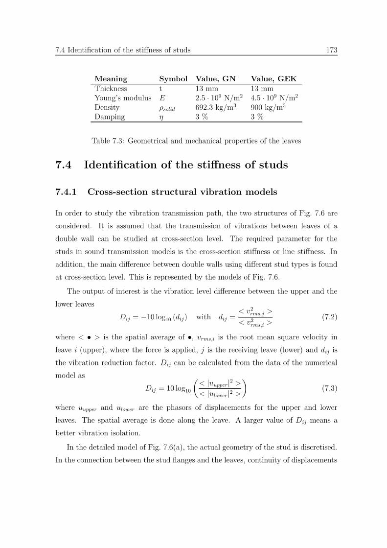
7.4 Identification of the stiffness of studs 173

Meaning Symbol Value, GN Value, GEKThickness t 13 mm 13 mmYoung’s modulus E 2.5 · 109 N/m2 4.5 · 109 N/m2

Density ρsolid 692.3 kg/m3 900 kg/m3

Damping η 3 % 3 %

Table 7.3: Geometrical and mechanical properties of the leaves

7.4 Identification of the stiffness of studs

7.4.1 Cross-section structural vibration models

In order to study the vibration transmission path, the two structures of Fig. 7.6 are

considered. It is assumed that the transmission of vibrations between leaves of a

double wall can be studied at cross-section level. The required parameter for the

studs in sound transmission models is the cross-section stiffness or line stiffness. In

addition, the main difference between double walls using different stud types is found

at cross-section level. This is represented by the models of Fig. 7.6.

The output of interest is the vibration level difference between the upper and the

lower leaves

Dij = −10 log10 (dij) with dij =< v2

rms,j >

< v2rms,i >

(7.2)

where < • > is the spatial average of •, vrms,i is the root mean square velocity in

leave i (upper), where the force is applied, j is the receiving leave (lower) and dij is

the vibration reduction factor. Dij can be calculated from the data of the numerical

model as

Dij = 10 log10

(< |uupper|2 >< |ulower|2 >

)(7.3)

where uupper and ulower are the phasors of displacements for the upper and lower

leaves. The spatial average is done along the leave. A larger value of Dij means a

better vibration isolation.

In the detailed model of Fig. 7.6(a), the actual geometry of the stud is discretised.

In the connection between the stud flanges and the leaves, continuity of displacements


and rotations is imposed. In the simplified model of Fig. 7.6(b), the stud is replaced

by a translational spring, a rotational spring and concentrated masses. The equiva-

lence between both models has been established by comparison of the vibration level

difference Dij.

For all the results presented here, four load configurations have been considered,

see Fig. 7.6(b). The positions of punctual loads have been chosen in order to be

representative: load applied over the stud or between studs, and at the centre of the

double wall or on the side. The study is done in terms of averaged responses: average

of the load position, average in time (over a period), average in frequency (the results

are given in third frequency bands) and average in space. Two different regions, the

upper and lower leaves, have been considered in order to perform space averages. One

analysis per Hz is carried out in order to describe the response spectrum; this implies

20 000 elastic calculations per case (case means, analysed section or analysed value of

stiffness in one of the three tests).

The structural spectral element method (see Doyle (1997) or Yu and Roesset

(2001)) has been chosen. In two-dimensional situations, the exact solution is reached

using only the necessary elements in order to describe the geometry (i.e. 5 elements

are required for the case of the TC cross-section, 9 for the AWS and 4 for the O). This

is a very important advantage since typical mesh requirements of the finite element

method can be forgotten. Results presented in Sections 7.4.2 and 7.4.3 are obtained

using this model.

7.4.2 Influence of stud shape in the vibration level difference

Fig. 7.7 is an example of the results obtained when comparing several sections. For

all of them, the isolation of vibrations in the low frequency range is really poor. It

cannot be improved by changing the stud shape. Note that standard sections like

TC, O or S provide an almost constant level of vibration isolation. On the contrary,

acoustic sections like LR or AWS improve the isolation of vibrations in the mid and

high frequency range (but they can be worse than the others for some frequencies in

the low frequency range).


M

F

relationship: u u ( )x y θ

(a)

F 3

K Kθt

M/2F 1 F 2 F 4

(b)

Figure 7.6: Models of the leave-stud-leave package: (a) detailed model with the actualgeometry of the studs; (b) simplified model with studs modelled as a translationalstiffness Kt, a rotational stiffness Kθ and two concentrated masses M/2. F i indicatesthe four load positions considered.

-5

0

5

10

15

20

25

30

35

1000

800

630

500

400

315

250

200

160

125

100

80

63

50

40

31.5

25

20

16

Dij

f (Hz)

AWSO

STC

LR

(a)

10

20

30

40

50

60

70

6300

5000

4000

3150

2500

2000

1600

1250

1000

Dij

f (Hz)

AWSO

STC

LR

(b)

Figure 7.7: Comparison of the vibration level difference for several studs with differentcross-section: (a) low-frequency range; (b) mid-frequency range. Note the differentvertical scales.


The vibration level difference Dij is a useful parameter in order to compare the

performance of different studs used in the same double wall. However, it is an

environment-dependent parameter: the values of Dij do not only depend on the stud

type. They also depend on other variables, such as leave properties and boundary

conditions. Thus, Dij is not a parameter characterising the stud. As shown in the

following sections, the stiffness of the stud is a better parameter, less dependent on

each particular situation and more related with every stud type.

7.4.3 Stud equivalent stiffness

A set of admissible values of rotational and translational stiffness can be obtained by

comparing the two deterministic models presented in Fig. 7.6. The key is to find pairs

of values that provide, for a given frequency, the same vibration level difference.

This requires to generate surfaces of vibration level difference in the plane Kt -

Kθ for every third frequency band. The surfaces obtained for 200, 500, 1000 and

3150 Hz and for test 2 are shown in Fig. 7.8. They have been generated analysing

36 different situations combining values of Kt = 104, 105, 106, 107, 108, 109 N/m2 and

Kθ = 101, 102, 103, 104, 105, 106 N · m/ (rad · m).

Once the surfaces have been generated, the admissible values of rotational and

translational stiffness can be obtained by imposing the same value of vibration level

difference for both models of Fig. 7.6:

D(simplified)ij (Kt, Kθ) = D

(detailed)ij (7.4)

Both the surface D(simplified)ij (obtained with the simplified model, see Fig. 7.8) and the

value D(detailed)ij (obtained with the detailed model) are known. The equality provides

a set of admissible values (Kt, Kθ), which yield the same vibration isolation in the

simplified model and the detailed model.

The values for the TC section and test 2 can be seen in Fig. 7.9. Three sets of

figures like these ones have been obtained for every section (one for each test).

Several important aspects have to be highlighted. On the one hand, an equivalent


0 10 20 30 40 50 60 70 80 90

f = 0200.0 Hz

10000 100000

1e+06 1e+07

1e+08 1e+09Kt [N/m2] 10

100

1000

10000

100000

1e+06

Kθ [N•m/rad•m]

0 20 40 60 80

100

Dij [dB]

0 10 20 30 40 50 60 70 80 90

f = 0500.0 Hz

10000 100000

1e+06 1e+07

1e+08 1e+09Kt [N/m2] 10

100

1000

10000

100000

1e+06

Kθ [N•m/rad•m]

0 20 40 60 80

100

Dij [dB]

0 10 20 30 40 50 60 70 80 90

f = 1000.0 Hz

10000 100000

1e+06 1e+07

1e+08 1e+09Kt [N/m2] 10

100

1000

10000

100000

1e+06

Kθ [N•m/rad•m]

0 20 40 60 80

100

Dij [dB]

0 10 20 30 40 50 60 70 80 90

f = 3150.0 Hz

10000 100000

1e+06 1e+07

1e+08 1e+09Kt [N/m2] 10

100

1000

10000

100000

1e+06

Kθ [N•m/rad•m]

0 20 40 60 80

100

Dij [dB]

Figure 7.8: Vibration level difference Dij in test 2 as a function of translationalstiffness Kt and rotational stiffness Kθ, for various frequencies.

effect in terms of Dij can be obtained using: i) only a translational spring; ii) only

a rotational spring; iii) and adequate combination of both. The option chosen here

is to use Kθ = 0 and a frequency-dependent Kt. On the other hand, a frequency

dependence of the parameters is observed. For low frequencies the values of stiffness

are smaller (around the typical values of elastic measurements), and they generally

increase with frequency.

For a given section, similar results are obtained for the three different tests. This

indicates that a steel stud can be characterised by parameters that not depend on

the environment (boundary conditions, leaves, symmetry of the double wall,...). In


1e+01

1e+02

1e+03

1e+04

1e+05

1e+071e+061e+051e+04

Kθ

[N•m

/rad

•m]

Kt [N/m2]

f = 200 Hzf = 250 Hzf = 315 Hzf = 400 Hz

f = 500 Hzf = 630 Hzf = 800 Hzf = 1000 Hz

1e+01

1e+02

1e+03

1e+04

1e+05

1e+071e+061e+051e+04

Kθ

[N•m

/rad

•m]

Kt [N/m2]

f = 1250 Hzf = 1600 Hzf = 2000 Hzf = 2500 Hz

f = 3150 Hzf = 4000 Hzf = 5000 Hzf = 6300 Hz

Figure 7.9: Admissible values of rotational and translational stiffness for the TCsection obtained by comparison of deterministic models. Test 2.

Fig. 7.10, the results of tests 1, 2 and 3 for the AWS section are compared. The

agreement is not perfect; however, the tendencies are correct. The lines corresponding

to the same frequency are close together. The dispersion is more important for low

frequencies, where the modal behaviour governs the response and the number of modes

in the third frequency band is smaller. In the low-frequency range (frequencies under

200 Hz) it is difficult to obtain this kind of laws. The values of D(simplified)ij oscillate

between 0 dB and 5 dB depending on the value of the stiffnesses and the mechanical

and geometrical characteristics of the leaves. Thus, the intersection of the D(simplified)ij

surface with a constant value D(detailed)ij does not provide smooth curves like in Fig. 7.9.

In Fig. 7.11 a typical final output for this kind of analysis can be seen. Frequency-

dependent translational stiffness laws are presented for every section.

7.5 Using the stiffness values in a SEA model

The values of stiffness characterising the sections can be used as input data for other

modelling techniques. A clear example is its use as input data for Statistical Energy

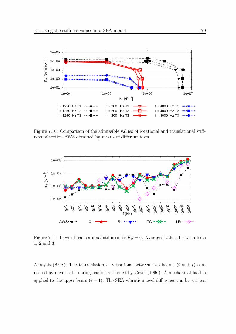
7.5 Using the stiffness values in a SEA model 179

1e+01

1e+02

1e+03

1e+04

1e+05

1e+071e+061e+051e+04

Kθ

[N•m

/rad

•m]

Kt [N/m2]

f = 1250 Hz T1f = 1250 Hz T2f = 1250 Hz T3

f = 200 Hz T1f = 200 Hz T2f = 200 Hz T3

f = 4000 Hz T1f = 4000 Hz T2f = 4000 Hz T3

Figure 7.10: Comparison of the admissible values of rotational and translational stiff-ness of section AWS obtained by means of different tests.

1e+05

1e+06

1e+07

1e+08

6300

5000

4000

3150

2500

2000

1600

1250

1000

800

630

500

400

315

250

200

160

125

100

KT (

N/m

2 )

f (Hz)

AWS O S TC LR

Figure 7.11: Laws of translational stiffness for Kθ = 0. Averaged values between tests1, 2 and 3.

Analysis (SEA). The transmission of vibrations between two beams (i and j) con-

nected by means of a spring has been studied by Craik (1996). A mechanical load is

applied to the upper beam (i = 1). The SEA vibration level difference can be written


as

Dij = D12 = 10 log10

(m2η2ω

|Y1 + Y2 + Yt|2nRe Y2

)(7.5)

where m2 is the mass per unit length, η2 is the loss factor, n is the number of con-

nections (springs) per unit length, Y1 and Y2 are the mobility of the two beams and

Yt is the mobility of a point connecting tie. The last parameter can be related to the

dynamic stiffness of this tie, Yt = v/F = iω/Kt, where Kt is the stiffness (in this SEA

model, only translational stiffness is considered), and v is the rate of length change

of the spring. For the mobility of the two beams, the formulas given in Cremer et al.

(1973) can be used

Y∞beam =1

4Ysemi-∞beam =

(1 − i)

4m`cBwith cB =

ω4

√ω2m`/E I

. (7.6)

m` is the density per unit length of the beam, E the Young’s modulus and I the inertia.

Note that two reference cases have been considered: infinite and semi-infinite beams.

The former provides better approximations for high frequencies where the influence

of boundaries is not important and the vibrations are localised due to damping. The

latter is a better approximation for low frequencies or situations where the mechanical

load is close to the boundary.

We have considered first the case of two beams connected by means of springs, see

Fig. 7.6(b). In this case the value of the stiffness is known and a ‘pure’ comparison

between the SEA model and the numerical method (SFEM) can be established with-

out additional errors caused by the uncertainties due to the characterisation of the

stud shape.

The results are presented in Fig. 7.12. The transmission of vibrations in test 2 has

been calculated with the numerical model and with the SEA model considering two

situations: infinite and semi-infinite beams. The agreement is correct. The numerical

results are closer to the infinite beam curve. Differences are smaller for mid and high

frequencies.

The modal behaviour at low frequencies is affected by the value of the stiffness.

For the smaller values of Kt, the two leaves are weakly connected and vibrations are

7.5 Using the stiffness values in a SEA model 181

20

30

40

50

60

70

80

90

100

6300

5000

4000

3150

2500

2000

1600

1250

1000

800

630

500

400

315

250

200

160

125

100

Dij

f (Hz)

Kt = 104 N/m2

0

10

20

30

40

50

60

70

80

6300

5000

4000

3150

2500

2000

1600

1250

1000

800

630

500

400

315

250

200

160

125

100

Dij

f (Hz)

Kt = 105 N/m2

-10

0

10

20

30

40

50

60

6300

5000

4000

3150

2500

2000

1600

1250

1000

800

630

500

400

315

250

200

160

125

100

Dij

f (Hz)

Kt = 106 N/m2

-5

0

5

10

15

20

25

30

35

40

6300

5000

4000

3150

2500

2000

1600

1250

1000

800

630

500

400

315

250

200

160

125

100

Dij

f (Hz)

SFEM

Kt = 107 N/m2

-4

-2

0

2

4

6

8

10

12

14

16

6300

5000

4000

3150

2500

2000

1600

1250

1000

800

630

500

400

315

250

200

160

125

100

Dij

f (Hz)

SEA inf

Kt = 108 N/m2

-4

-2

0

2

4

6

8

10

12

14

6300

5000

4000

3150

2500

2000

1600

1250

1000

800

630

500

400

315

250

200

160

125

100

Dij

f (Hz)

SEA semi-inf

Kt = 109 N/m2

Figure 7.12: Two leaves connected with springs. Comparison of the vibration leveldifference obtained by means of a numerical model (SFEM) and statistical energyanalysis. Note the different scale for Dij.


developed all along the span length (3 m). Nevertheless, for larger values ofKt the link

between leaves becomes stronger, and each leave cannot be considered as a 3 m long

beam. Due to the connections it behaves like a group of short cells (space between

springs). Oscillations in the response curve are then important for frequencies below

400 Hz (Kt = 107 N/m2), 2000 Hz (Kt = 108 N/m2) and 4500 Hz (Kt = 109 N/m2).

Results presented here are also important in order to understand the type of laws

obtained for the translational and rotational stiffnesses. The values of Dij for some

of the studied sections have an small variation range. See for example the variation

of O, TC and S studs in Fig. 7.7(b), where the values of Dij are between 15 and

35 dB. On the contrary, the variation range of Dij for some cases of constant spring

stiffness is very large (see Fig. 7.12, Dij ∈ [25, 90] for Kt = 104 N/m2, Dij ∈ [10, 80]

for Kt = 105 N/m2, Dij ∈ [0, 60] for Kt = 106 N/m2 . . .). This means that the studied

sections behave like a spring of variable, rather than constant, stiffness. If the required

stiffness was constant, the variation of Dij obtained with the model considering the

geometry of the stud would be larger. This is not the case.

The same method has been used for the case where the two leaves are connected

by means of steel studs, see Fig. 7.6(a). In this case, two different errors are possible.

On the one hand the agreement between a SEA model and a numerical model (shown

with the previous example). On the other hand, the correct characterisation of steel

studs (Kt − f laws).

The results for AWS and TC studs are presented in Fig. 7.13. Again the vibration

level difference calculated by means of a numerical model and by means of the SEA

model is compared. Now, for the case of the SEA model, the value of stiffness is

variable with frequency. The laws obtained in Section 7.4.3 have been used as input

data.

This example shows how the double wall behaviour predicted by a model that

considers the geometrical detail of the studs can be reproduced by means of a SEA

model, where the geometrical complexity has been reduced to the use of a frequency-

dependent stiffness law.

7.6 Global response of double walls 183

0

10

20

30

40

50

60

70

6300

5000

4000

3150

2500

2000

1600

1250

1000

800

630

500400

315

250200160

125100

Dij

f (Hz)

SFEM

(a)

0

10

20

30

40

50

60

70

6300

5000

4000

3150

2500

2000

1600

1250

1000

800

630

500400

315

250200160

125100

Dij

f (Hz)

SEA infinite

(b)

Figure 7.13: Comparison of vibration level difference obtained by i) a detailed nu-merical model where the actual geometry of the studs is discretised (SFEM) and ii)a SEA model, which uses a frequency-dependent stiffness provided by the numericalmodel: (a) acoustic stud AWS; (b) standard stud TC.

7.6 Global response of double walls

In previous sections the effort has been focused on the characterisation of flexible steel

studs and the study of the vibration transmission path (vibration level difference). It

is only one of the parts of the problem of sound transmission. The performance of

the studs and the validity of results obtained in Section 7.4 is now verified in a two-

dimensional vibroacoustic problem. This means that both the stud path and the

cavity path are considered at the same time, see Fig. 7.1.

The relevance of acoustic design of studs depends on the type of double wall. If

the cavity path is very insulating, the stud path will be the critical path and then the

type of stud used is very important. On the contrary, if the isolation of the cavity

path is poor, the type of stud used will not be relevant because most of the sound is

not transmitted through the stud.


The effect of mechanical connections between leaves has been studied in Sec-

tion 6.6.2. The main conclusion is that there are limit values of stiffness below and

above which the effect of the stud is not important. These limit values depend on the

type of double wall (separation between leaves, use or not of absorbing material, type

of leaves). If the modifications in the stud (shape, thickness, materials, damping) can

change its stiffness in this frequency range the optimisation is possible, otherwise the

type of stud used is not an important variable of the problem.

The model presented in Chapter 5 has been used. The studs have been considered

now, see the finite element mesh of Fig. 7.14. Two rectangular acoustic domains, the

two leaves connected by means of a steel stud and the cavity between leaves can also be

seen. The dimensions of the rooms are 5.7 m × 4.7 m and 6.35 m × 5 m. The double

wall is 3 m long. For some cases absorbing material (resistivity % = 8000 Pa · s/m2) is

placed inside the air cavity. The cavity has been considered continuous through the

studs. The opposite situation where small cavities between the studs are modelled

instead of a large single cavity can also be reproduced with the numerical model.

However, the thermal slots in the studs web establish a continuity in the air between

leaves that justifies the use of a single air cavity. A sound source has been placed in

the lower left corner of the sending room (separated 0.5 m from each wall). The value

of impedance in Robin contours is Z/ (ρ0c) = 19.03.

In Fig. 7.15 the sound level difference for the 0.07 m thick double wall with and

without absorbing material in the cavity can be seen. Several values of translational

stiffness have been considered. The limit values for this double wall are 105 N/m2 and

108 N/m2. It can be seen that the improvement by the use of flexible studs is larger if

there is absorbing material in the cavity (high cavity path isolation) than in the case

of air cavity (poor cavity path isolation).

Fig. 7.16 shows the results obtained from the vibroacoustic model where the springs

have been replaced by studs. A set of TC studs with increasing value of thickness

(0.00047 m, 0.001 m and 0.003 m) have been considered. The translational stiffness

laws obtained by means of the analysis presented in Section 7.4 for these TC studs

and the sound level difference of every section can be seen in Fig. 7.16(a). The value

7.6 Global response of double walls 185

(a) (b)

Figure 7.14: Finite element mesh used to solve the vibroacoustic problem: (a) generalview of the two rooms and the double wall; (b) detail in the double wall zone.

10

20

30

40

50

60

70

80

2500

2000

1600

1250

1000

800

630

500

400

315

250

200

160

125

100

80 63 50 40 31.5

25 20 16

D (

dB)

f (Hz)

Kt <= 105 N/m2

Kt = 106 N/m2Kt = 107 N/m2

Kt >= 108 N/m2

(a)

10

20

30

40

50

60

70

80

2500

2000

1600

1250

1000

800

630

500

400

315

250

200

160

125

100

80 63 50 40 31.5

25 20 16

D (

dB)

f (Hz)

Kt <= 105 N/m2

Kt = 106 N/m2Kt = 107 N/m2

Kt >= 108 N/m2

(b)

Figure 7.15: Influence of the value of translational stiffness Kt (Kθ = 0). Sound leveldifference D: (a) double wall with air cavity; (b) double wall with absorbing material.Thickness of double wall: d = 0.07 m.


of sound level difference provided by every stud is coherent (comparing Kt − f laws

and isolation of double walls with springs). Taking, for example the 0.001 m thick TC

stud, it can be seen in Fig. 7.16(a) that its Kt−f law goes from values under 107 N/m2

to values close to 108 N/m2. Fig. 7.16(b) shows that the sound level difference curve

of this stud also goes from values under the Kt = 107 N/m2 curve to values that are

close to the Kt = 108 N/m2 curve.

1e+06

1e+07

1e+08

1e+09

6300

5000

4000

3150

2500

2000

1600

1250

1000

800

630

500

400

315

250

200

Kt (

N/m

2 )

f (Hz)

0.00047 m0.001 m

0.003 m

(a)

30

40

50

60

70

80

2500

2000

1600

1250

1000

800

630

500

400

315

250

200

160

D (

dB)

f (Hz)

e = 0.00047 me = 0.001 me = 0.003 m

Kt = 106 N/m2

Kt = 107 N/m2

Kt = 108 N/m2

(b)

Figure 7.16: Influence of the thickness e of the studs: (a) Kt− f laws for a set of TCstuds; (b) sound level difference of a double wall with TC-studs and with springs ofconstant stiffness.


The influence of the stud type in the vibration transmission between leaves of a double

wall have been shown in Section 7.4.2. The results are dependent on many factors

like: local resonances; mechanical properties of materials that are always important

at least in some frequency range; type of link between the leaves and the studs. This


variability of the results is a found all along the study. However, it can be concluded

that some sections like AWS and LR provide a slightly better isolation of vibrations

than more usual sections (S,TC and O). The improvement is more important for

high frequencies. For low frequencies the difference of Dij between stud shapes is

small. Moreover it has no practical relevance if the entire vibroacoustic problem is

considered, see the low-frequency response in Fig. 7.15.

Two reasons explain the improvement in the isolation of vibrations of acoustic

studs. On the one hand, they are more flexible due to their cross-section shape.

However, this intuitive increase of flexibility is only true around the eigenfrequencies

where the central part of the stud acts as a spring, see Fig. 7.17(a). On the other hand,

acoustic studs have a larger perimeter. This represents an increase of the effective

damping in the vibration transmission path from the upper to the lower parts of the

stud. This is mainly relevant for high frequencies where the length of vibration waves

is smaller than a characteristic length of the stud. The displacements are small but

fast and dissipation is more relevant. This is the case of Fig. 7.17(b). The increase

of the vibration isolation in this frequency range could also be achieved by means of

some damping mechanism in the stud (i.e. use of materials with high damping). This

has not been considered here.

A methodology for the characterisation of studs has been presented. They can be

modelled by means of a translational spring with a frequency-dependent stiffness law.

In all the sections analysed the stiffness increases with frequency. These frequency-

dependent laws have been successfully used in SEA models of beams connected by

means of springs.

The effect of the stiffness of the spring connecting leaves of several double walls

has been studied. There are a minimum and a maximum value of stiffness below and

above which the isolation capacity of the wall is not modified. These two characteristic

values of the wall determine if it is important or not to improve the flexibility of the

stud. There is also a threshold of frequency below which the response of the wall is

not controlled by the stiffness of the connecting elements.

A comparison with the sound level difference of walls with springs between leaves


0 1.1e-06 2.2e-06

|u| f=50 Hz

(a)

0 4e-09 8e-09

|u| f=2000 Hz

(b)

Figure 7.17: Different vibration shapes of a TC stud placed between leaves (zoom ofthe entire package): (a) f = 50 Hz, the stud vibrates by separating its upper andlower parts like an spring; (b) f = 2000 Hz, the vibration wave length is shorter thanthe stud.

and walls with studs has been done. The sound level difference curve of the double

walls with studs crosses the sound level curves of constant spring stiffness value. This

means that the stiffness of the stud is increasing with frequency. The behaviour is

correctly predicted by the obtained frequency-dependent stiffness laws.

Chapter 8

Numerical modelling of flanking

transmissions

8.1 Introduction

The sound transmission loss of building walls measured in the field (i.e. apartments,

offices, industries...) is often smaller than expected results. One of the possible

causes of a poor field response of an element with good properties in the laboratory

are flanking transmissions. That is, the indirect transmission of sound from one room

to another through any part of the building that is in contact with the wall (other

walls, floors, pipes,...). Prediction models and laboratory measurements usually deal

with an individual wall and only direct transmissions are considered.

Field measurements of flanking transmissions have been reported in the literature.

In Fothergill (1980) some real situations of apartments with poor sound isolation

properties are described. The cause is in most of them the existence of transmission

paths not considered during the design phase. The final solutions and measurements

showing the improvement (if possible) are shown for each case. Another example of

apartment affected by indirect transmission is shown in Hongisto (2001). Intensity

measurement methods are employed in order to characterise the transmission path.

This experimental technique not only provides spatial averaged information for every

189

190 Numerical modelling of flanking transmissions

room (pressure) but also qualitative information in the sense that the zones with

higher acoustic intensity can be characterised. Intensity methods have also been

used by van Zyl et al. (1986) in order to avoid the influence of flanking paths in

sound reduction index measurements. In Esteban et al. (2006) the effect of flanking

transmissions in buildings made of masonry walls is shown. The discussion is focused

on a paradoxical situation where the heaviest wall does not provide the highest sound

transmission loss. The increase of mass is, in that particular situation, positive from

the point of view of direct transmissions but negative for indirect transmissions. The

best solution is an intermediate wall with adequate properties for both types of sound

transmission.

The accurate modelling of flanking transmissions requires the consideration of

structural paths of vibration transmission. This can be done by means of simple

devices or coefficients connecting simplified structural elements (such as semi-infinite

plates) or by performing a detailed description of the structure. The importance

of construction details and boundary conditions is a significant challenge from the

modelling point of view. Due to the difficulties of sound transmission modelling,

these aspects are often simplified in the study of direct transmissions. This is not

valid for the case of indirect transmissions. In addition, the size of the problems is

increased due to the consideration of larger and more complex structures.

The number of available models for flanking transmission is not large, especially

when compared with models developed for direct sound transmission through single

and double walls. In Craik (2001), statistical energy analysis is used in the study of

long structural paths of sound transmission in buildings. A SEA model is also devel-

oped in Guyader et al. (1986). It is used in the modelling of a laboratory experimental

set-up. Theoretical results are compared with measurements with good agreement.

Experimental measurements in a flanking laboratory where different walls have an in-

tentional flanking path (transmission between floors) are reported in Hopkins (1997).

In Craik et al. (1997), a wave approach model is developed. Wave approaches are

based on the assumption of infinite or semi-infinite structures. Thus, this model is

limited to the study of a junction instead of an entire building or laboratory. The


transmission of vibrations through an X-shaped junction involving a double wall is

calculated and used for the prediction of sound transmission. The data obtained by

means of the wave approach model is then used in a SEA model that considers both

airborne and structural paths. Numerical-based models have also been used in order

to predict flanking transmissions. In Clasen and Langer (2007), results obtained by

means of a two-dimensional finite element model have been compared with laboratory

measurements. The measurements have been done in a reduced scale laboratory. The

numerical model has been used in order to model in detail the junctions between the

floors and the walls. It has been shown that using elastic materials can improve the

isolation of the flanking paths.

The most global model for flanking transmissions is the one presented in Gerretsen

(1979) and Gerretsen (1986). The formulation is based on parameters characterising

the individual building components (sound reduction index, radiation efficiency and

surface of the partitions). The information of the relationship between the components

of the building that are in contact is reduced to a single parameter, the vibration

reduction factor (transmission of vibrations between floors, adjacent walls, floors and

walls,...). This model is the basis of the European regulation EN-12354 (2000). More

details will be given in the following sections since this code will be compared with

numerical results. The model is also assumed with minor modifications by some

national standards, which is the case of Spain in the new building regulation (CTE

(2007)). Field measurements are being done in order to ensure that the European

standard is also valid for the typical type of Spanish buildings (made of masonry or

stone), see Esteban et al. (2003). More simplified models are also assumed by other

regulations, Szudrowicz and Izewska (1995).

The numerical model presented in Chapter 5 has been used in order to predict

flanking transmissions in the case of acoustic excitation. Since the structure is mod-

elled by means of finite elements, both structural details and links (boundary con-

ditions) between walls can be considered. All the calculations presented here have

been done using a three-dimensional version of the model. In Section 8.3 some junc-

tions between monolithic structural elements will be analysed. A good and a poor


acoustic design of the junction between a double wall and a floor will be modelled in

Section 8.4.

8.2 The flanking transmission model of EN 12354

The more basic aspects of the EN 12354 model will be reviewed here. The goal of

this section is only to outline the simplified model used to compare with the obtained

numerical results. For a more detailed description of the model, the original papers

by Gerretsen (1979), Gerretsen (1986) or more recent discussions of the model like

Nightingale (1995) should be checked. The practical use of the model is described in

EN-12354 (2000) or CTE (2007).

The entire structure (building) is understood as an assembly of smaller structures

(typically walls and floors). The main assumption is that the total transmitted sound

is the addition of the sound transmitted through each of the paths (from one structure

to another). It is also assumed that there is no interaction between different paths (the

transmission of sound and vibrations through a given path is completely independent

from the others). Two important aspects in order to perform accurate predictions

are to correctly define the division of the building into structures and to identify

each transmission mechanism. The second aspect can depend on construction details

and more than one transmission path should be considered between two structures if

necessary (i.e. transmission from floor to floor due to structural continuity but also

due to passing pipelines).

The incident acoustic power in structure i caused by an acoustic excitation in the

sending room (reverberant field) can be expressed as WInc,i = Si⟨p2rms,s

⟩/4ρ0c. Si is

the surface of structure i,⟨p2rms,s

⟩is the mean pressure level in the sending room, ρ0

is the density of air and c the speed of sound in air. The power radiated by structure

j due to the excitation of structure i (caused by the pressure field in the sending

room) can be expressed as Wrad,j = ρ0cSjσj⟨v2rms,ij

⟩. σj is the radiation efficiency of

structure j and vrms,ij is the averaged root mean square velocity in structure j due to

the vibration of structure i. In the global problem the velocity of structure j is the

8.2 The flanking transmission model of EN 12354 193

addition of the velocities of each path ij, v2rms,j =

∑i v

2rms,ij .

The key idea of the model is to express Wrad,j as a function of the pressure in

the sending room. With this goal, the vibration transmission factor is defined as

dij = v2rms,j/v

2rms,i (j is the receiving structure and i the excited one). It characterises

the vibration path between structures i and j. The contribution to the pressure field in

the receiving room due to the transmission path ij,⟨p2r,ij

⟩, as well as the transmission

factor for path ij, can be expressed as

⟨p2r,ij

⟩=σjSjdij

⟨p2rms,s

⟩

σiAreceivingand τij =

Wrad,j

Winc,i

=σjSjdijτiσiS0

(8.1)

where Areceiving is the absorption in the receiving room, τi the sound reduction index

of structure i, and S0 the surface area of the element defining the direct transmission

path. The sound reduction index of path ij can then be expressed as

Rij := 10 log10

(1

τij

)= Ri +Dij + 10 log10

(σiσj

)+ 10 log10

(S0

Sj

)(8.2)

where Ri := 10 log10 (1/τi) is the sound reduction index of structure i and Dij =

−10 log10 (dij) the vibration level difference.

Historically, reciprocity (Rij = Rji) has been assumed. Thus, the radiation effi-

ciencies can be suppressed from the formula

R =1

2(Rij +Rji) =

1

2(Ri +Rj) +

1

2(Dij +Dji) + 10 log10

(S0√SiSj

)(8.3)

The averaged vibration level difference is maybe the key parameter in order to ac-

curately predict flanking transmissions. Since Dij depends on the damping and di-

mensions of the structure, standards tend to use the more environment-independent

vibration reduction index

Kij = Dν,ij + 10 log10

(`ij√aiaj

)with Dν,ij =

1

2(Dij +Dji) (8.4)

where `ij is the length of the junction and ai the characteristic absorption length of


structure i. An accepted approximation is to use ai = Si/L0 and L0 = 1 m. This

assumption is used in order to calculate Dν,ij . More accurate prediction formulas for

the characteristic length can be found for example in Crispin et al. (2006). The aim is

that Kij depends only on the junction type (shape) and the density and thicknesses

of the adjoint elements, and not on the particular dimensions and damping of the

structure.

Empirical expressions of Kij for several junction types are provided in the regu-

lation EN-12354 (2000). The transmission of vibrations through junctions has also

been modelled using a wave approach and compared with experimental data in Ped-

ersen (1995). This model has been largely applied for the prediction of flanking paths

in heavy monolithic constructions. In those cases, the critical frequency is low and

the sound transmission is mainly resonant. During the last years several comparisons

between the model proposed in the regulation and empirical measurements have been

published. Some of them have been summarised in Table 8.1. A brief description

of the measurement type, main results obtained and causes of discrepancy have also

been included. More details can be found on the cited references. This is especially

important in the field of flanking transmissions where small modifications of the input

data cause large variations of the final outputs.

Predictions can be inaccurate for the case of lightweight constructions. As dis-

cussed in Nightingale (1995), Guigou-Carter et al. (2006) and Villot (2002), indirect

transmissions are mainly a resonant phenomenon (the forced excitation of structures

by means of a coincident pressure field does not cause flanking transmissions). The

laboratory measurements of sound reduction index of individual elements (as well

as the data provided by models on sound transmission) include both the resonant

and the forced components. Data considering only the resonant component would be

necessary. Since it is often not available or not considered in usual expressions, the

EN 12354 model for flanking transmissions can underestimate the sound reduction

index of the flanking paths (especially below the critical frequency). Note that the

transmission factor of the excited structure τi is used in Eqs. (8.1) and (8.2).

In the following sections, the simplified model results (labelled EN in the plots)

8.2 The flanking transmission model of EN 12354 195

Reference Type Mat. Parameter Diff. (dB) Reason• Metzen (1999) I H, L R 2.0 ± 1.8 I, D, S• Pedersen (1999) I H, L R, Ln H : 0.3 ± 2.2

L : 0.25 ± 3.1• Esteban et al. (2003) I B Ki,j: X,T,E −2 to −10 S• Crispin et al. (2006) S C Ki,j: X,T,E −3.5 to 2 M, W• Galbrun (2007) FL C, B Di,j −1 to 5 L, I, D

Table 8.1: Recent published comparisons between EN 12354 and empirical data.Type of measurement (Type): in situ (I), flanking laboratory (FL), isolated structuralelement (S). Structure material (Mat.): heavy structures in general (H), lightweightstructures (L), concrete (C), hollow bricks (B). Analysed parameters (Parameter):vibration level difference (Di,j), vibration reduction index (Ki,j: X, T, L, H indicatethe junction type and E if elastic layer is considered for some of them), sound reductionindex (R), impact noise (Ln). The difference (Diff.) is always: predicted by EN 12354minus measured. Reason of discrepancies between predictions and measurements(Reason): consideration of details at junction level are necessary (D), the structure isnot monolithic (S), the modal density of the tested elements is low (M), long flankingpaths should be considered (L), an improvement of the input data is necessary (I),effect of workmanship (W).

are obtained using the expression

R =1

2(Ri +Rj) +Kij + 10 log10

(S0

`ijL0

)(8.5)

The sound reduction index of individual elements can be calculated by means of

the formulas discussed in Section 6.2 or in Beranek and Ver (1992), Josse (1975),

Fahy (1989) or Hongisto (2006). Most of the expressions found in the literature

mainly consider forced transmission. Their use leads to underestimation of the sound

reduction index on indirect paths in lightweight structures, especially for frequencies

below the critical frequency.


8.3 Sound transmission in rigid junctions

Different junction types have been analysed: L-shaped, T-shaped and X-shaped.

Rigid junctions have been considered. All the structures that coincide in the junction

are monolithic elements. Details like the existence of a pipeline or more complex

junction types (i.e. junctions with steel beams and plasterboards that are screwed)

have not been included in the analysis. In all the situations, the numerical results

are compared with the solutions obtained using the model described in Section 8.2.

The sound transmission between two rooms (L and T junctions) or four rooms (X

junction) is calculated. In Fig. 8.1 sketches and notation of the analysed situations

can be seen. The dimensions of the rooms are listed in Table 8.2.

Room 1 (and 4) Room 2 (and 3)Junction `x `y `z `x `y `z

L-shaped 2.24 2.56 2.4 2.64 2.56 2.4T-shaped (1st) 2.24 2.56 2.4 2.64 2.56 2.4T-shaped (2nd) 2.8 3.2 3 3.3 3.2 3X-shaped 2.5 2 2.3 2.8 2 2.3

Table 8.2: Room dimensions (in m) in each analysed situation.

All the calculations presented here have been carried out using a three-dimensional

numerical model. To the author’s knowledge, such three-dimensional simulations have

not been previously reported. The structure is modelled by means of finite elements

and the acoustic domains using modal analysis (see Chapter 5 for more details). The

sending room is room 1 (R1) in all cases. The absorption in all the rooms is α = 20 %.

The displacements in the contour of the structure are blocked. The material properties

for every case have been listed in Table 8.3. These values have been chosen in order to

maximise the effect of transmission paths according to the available empirical formulas

(minimise the vibration reduction index). In actual constructions there usually are

more differences between the stiffnesses and masses of orthogonal structures (floors

and walls).

In the case of the L-shaped junction, heavy and lightweight materials have been

considered. Thus, results for situations where the resonant transmission is predomi-

8.3 Sound transmission in rigid junctions 197

lylx

lz

!!!!!!!!!!!!!!!!!!!!!!!!!!!!!!!!!!!!!!!!!!!!!!!!!!!!!!!!!!!!!!!!!!!!!!!!!!!!!!!!!!!!!!!!!!!!!!!!!!!!!!!!!!!!!!!!!!!!!!!!!!!!!!!!!!!!!!!!!!!!!!!!!!!!!!!!!!!!!!!!!!!!!!!!!!!!!!!!!!!!!!!!!!!!!!!!!!!!!!!!!!!!!!!!!!!!!!!!!!!!!!!!!!!!!!!!!!!!!!!!!!!!!!!!!!!!!!!!!!!!!!!!!!!!!!!!!!!!!!!!!!!!!!!!!!!!!!!!!!!!!!!!!!!!!!!!!!!!!!!!!!!!!!!!!!

"""""""""""""""""""""""""""""""""""""""""""""""""""""""""""""""""""""""""""""""""""""""""""""""""""""""""""""""""""""""""""""""""""""""""""""""""""""""""""""""""""""""""""""""""""""""""""""""""""""""""""""""""""""""""""""""""""""""""""""""""""""""""""""""""""""""""""""""""""""""""""""""""""""""""""""""""""""""""""""""

########$$

%%%%%%%%%%%%%%%%%%%%%%%%%%%%%%%%%%%%

&&&&&&&&&&&&&&&&&&&&&&&&&&&&&&''''''''''''''''''((((((((((((((((((((

))))))))))))))))))))))))))))))))))))))))))

********

++++++++

,,,,,,,,

------------------------------

...................................

////////

00000

11111111111111111111111111111111111

2222222222222222222222222222222222222222222222222222222222222222222222222222222222222222222222222222222222222222222222222222222222222222222222222222222222222222222222222222222222222222222222222222222222222222222222222222222222222222222222222222222222222222222222222222222222222222222222222222222222222222222222222222222

333333333333333333333333333333333333333333333333333333333333333333333333333333333333333333333333333333333333333333333333333333333333333333333333333333333333333333333333333333333333333333333333333333333333333333333333333333333333333333333333333333333333333333333333333333333333333333333333333333333333333333333333333333333333333333

44444444

5555555555555555555555555555555555556666666 7777777777

8888888888

999999999999999999::::::::

;;;;;;;;

<<<<<<<<<<<<<<<<<<<<

====================>>>>>>>>?????????????????????????????? @@@@@@@@@@@@@@@@@@@@

AAAAAAAAABBBBBBBB

CCCCCCCCCCCCCCCCCCCCCCCCCCCCCCCCCCCCDDDDD

EEEEEEEEEEEEEEEEEEEE FFFFFFFFFFFFFFFFFF

GGGGGGGGGGGGGGGGGGGG

HHHHHHHHHHHHHHHHHHHH

IIIIIIIIIIIIIIIIIIIIIIIIIIIIII

JJJJJJJJJJJJJJJJJJJJJJJJJJJJJJJJJJJJJJJJJJJJJJJJJJJJJJJJJJJJJJJJJJJJJJJJJJJJJJJJJJJJJJJJJJJJJJJJJJJJJJJJJJJJJJJJJJJJJJJJJJJJJJJJJJJJJJJJJJJJJJJJJJJJJJJJJJJJJJJJJJJJJJJJJJJJJJJJJJJJJJJJJJJJJJJJJJJJJJJJJJJJJJJJJJJJJJJJJJJJJJJJJJJJJJJJJJJJJJJJJJJJJJJJJJJJJJJJJJJJJJJJJJJJJJJJJJJJJJJJJJJJJJJJJJJJJJJJJJJJJJJJJJJJJJJJJJJJJJJ

KKKKKKKKKKKKKKKKKKKKKKKKKKKKKKKKKKKK

R1R2

L−shaped (B)

X−shaped

L−shaped (A)

T−shaped

R1

R1

R4

R315

3

4 6

2

R1

R2F

D d

D d

f F f

D d

R2

Ff

R1−Dd−R2

R2dD

R1−Ff−R3

U u

DfDd

Fd

Ff

Df

Dd

Fd

Dd

R1−Fu−R3

Figure 8.1: Cases analysed (and notation) of rigid monolithic junctions.

Junction Structure E (N/m2) ρsolid (kg/m3) η (%) thickness (m)

L-shaped (heavy) A, B F, f, D 2.943 · 1010 2500 3 0.06L-shaped (lightweight) A, B F, f, D 4.8 · 109 913 3 0.03T-shaped (heavy) A F, f 2.943 · 1010 2500 1 0.06T-shaped (heavy) A D 2.943 · 1010 2500 1 0.10T-shaped (heavy) B F, f, D 2.943 · 1010 2500 1 0.10T-shaped (heavy) C D 2.943 · 1010 2500 1 0.06T-shaped (heavy) C F, f 2.943 · 1010 2500 1 0.10X-shaped (heavy) F, f, D, U 2.943 · 1010 2500 3 0.05

Table 8.3: Geometric and mechanical data of each structural zone.

nant (low critical frequency for heavy structures) and for situations where the forced

transmission is dominant (high critical frequency for lightweight structures) will be

obtained. Two different floor positions are possible: floor over the sending room (A)

or floor over the receiving room (B). In both cases, there is a direct path (Dd) and


a flanking path (case A: Fd; case B: Df). The face 4 of the cuboid without fluid-

structure interaction is purely reflecting. It is the only surface that is not in contact

with a structure and has no absorption along all the analysis.

For the case of the T-shaped junction, only heavy structures have been considered

but two sets of room dimensions have been used. The aim is to check the effect of

small modifications in room dimensions for the flanking transmission problem. Three

different situations regarding the mass ratio between the floors (F,f) and the wall

(D≡d) have been taken into account: A, with lighter floors; B, where the floors and

the wall have the same thickness and mechanical properties and finally C, with heavier

floors.

Finally, for the case of the X-shaped junction, the interest has been focused on

the sound transmission caused only by indirect flanking paths. It is the case of

transmission between rooms 1 and 3. The flanking paths analysed in detail are those

that begin at the first floor (F): R1-Fu-R3 and R1-Ff-R3. Only heavy structures have

been considered and the room dimensions have been slightly diminished in order to

reduce computational costs.

One of the advantages of a numerical model is the possibility of studying situations

that are virtual modifications of the reality (i.e. boundary conditions can be easily

modified in the numerical model while it is difficult in a building). Each transmission

path can be modelled separately. This facilitates the understanding of the physical

phenomenon. Table 8.4 is a summary of the coupling boundary conditions used for

each junction type and for each analysed path. The ‘Complete’ situation is the actual

one. A building or a laboratory where there is interaction between each structure

and all the contiguous acoustic domains. On the contrary, in situations named Fd,

Dd, Df, R1-Ff-R3, . . . only some flanking path is allowed. Note that the sending and

receiving rooms are only indicated for the case of an X-shaped junction. The path

R1-Ff-. . . can generate sound in rooms 2 and 3.

For example, in the second row of Table 8.4, ‘L-shaped A Fd’, an L-shaped junction

in the configuration A (floor over the sending domain) is analysed. The allowed path

is the Fd since we can see that the sending acoustic domain is coupled with the floor F


but not with the wall face D. The receiving acoustic domain is coupled with the wall

face d. Then, the only possible path is: acoustic excitation of floor F in the sending

room, vibration transmission to the wall d which radiates sound into the receiving

room. Similar interpretations can be done for the other examples analysed. The

outputs obtained in this incomplete problems are the sound reduction index Rij of

the path and the vibration level difference Dij.

The notation used in the figures showing the numerical results is illustrated by the

following example:

T-B F-f DF,d (8.6)

Three items are identified: where three item make possible the definition of the anal-

ysed situation:

1. Structure analysed. In that example the T-shaped junction with the material

properties B (T-B). The other possibilities are: L-A, L-B, T-A, T-B, T-C and

X.

2. Flanking path allowed (fluid-structure boundary condition). In that example

transmission through the floor (Ff). The first symbol is always related with the

sending room and the second one with the receiving room. The notation deals

only with the structural parts of the path, see Fig. 8.1.

3. Finally, the type of output calculated is shown. This can be the sound reduc-

tion index or the vibration level difference. In the example, the vibration level

difference between the first floor F and the wall d has been calculated. Note

that for the case of the X-shaped junction the notation U,u is introduced for the

upper wall. All the reference values obtained from the EN 12354 or the Spanish

technical code are indicated with EN or CTE respectively (the mass-law type

expressions found in Fahy (1989); Beranek and Ver (1992) are used for the direct

paths). For the case of sound reduction index, the situations where the total

sound reduction index (all the possible paths are considered and contribute to

the final value) has been calculated, have the subindex of the sending and re-

ceiving rooms (i.e. RR1,R2). For the cases of the sound reduction index of an


individual path, the structural elements defining the path are used as subindices

(i.e. RF,u).

Junction Case Room Coupling Room Couplingfaces faces

L-shaped A Complete 1 3, 4 2 1L-shaped A Fd 1 4 2 1L-shaped A Dd 1 3 2 1L-shaped B Complete 1 3 2 1, 4L-shaped B Df 1 3 2 4L-shaped B Dd 1 3 2 1T-shaped Complete 1 3, 4 2 1, 4T-shaped Ff 1 4 2 4T-shaped Fd 1 4 2 1T-shaped Df 1 3 2 4T-shaped Dd 1 3 2 1X-shaped Complete 1 3, 4 2 1, 4

3 1, 2 4 2, 3X-shaped S0 = D, R1-Ff-R2 1 4 2 4X-shaped S0 = D, R1-Fd-R2 1 4 2 1X-shaped S0 = D, R1-Df-R2 1 3 2 4X-shaped S0 = D, R1-Dd-R2 1 3 2 1X-shaped Only Flk, R1-Ff-R3 1 4 3 2X-shaped Only Flk, R1-Fu-R3 1 4 3 1

Table 8.4: Definition of the allowed flanking paths and boundary conditions in eachsituation.

8.3.1 L-shaped junctions

The vibration reduction index in the corner of a structure (L-shaped) can be predicted

using the following formula proposed in CTE (2007):

Kij = max (15|M | − 3,−2) (dB) with M = log10

((ρsurf)⊥i(ρsurf)i

)(8.7)

(ρsurf)i is the surface density of the excited structure i and (ρsurf)⊥i is the surface

density of the orthogonal structure (in the case of an L-shaped junction, the structure

j). Eq. (8.7) will be used in the simplified calculation of all transmission paths.

In Fig. 8.2, the results obtained for the heavy structure are plotted. The vibration


level difference is quite constant with frequency and no large differences exist between

paths (reciprocity can be assumed). However, the numerical values are considerably

larger than the values obtained with the simplified model (2 to 8 dB higher). This

causes important differences in the sound reduction index of the indirect paths. While

in the numerical model the difference between direct and indirect paths is around 8

dB, the simplified model predicts differences around 4 dB. With these numerical val-

ues, the effect of the flanking path can be neglected and cases A and B are equivalent.

Moreover, numerical isolation predictions for a single path are also higher than the

classical predictions using equations Eqs. (6.4), (6.5) and (6.9) (this has also been

seen in Chapters 5 and 6). This is caused, on the one hand, by the discrepancy fi-

nite structure/infinite structure, especially important at low frequencies. The effect

of the finite size of panels on the sound reduction index has been studied in Kernen

and Hassan (2005) and differences around 3 dB have also been found. On the other

hand, Eq. (6.5) especially takes into account the effect of coincidence. In heavy finite

structures with low critical frequency, a pure coincidence would rarely be found. Low

modal densities (limited number of wave types) as well as different boundary condi-

tions for the structure (supported, Dirichlet) and for the air pressure (low absorption

and almost purely reflecting acoustic boundaries) makes it difficult to find perfectly

matching pressure and displacement waves.

The same comments are valid for the case of the lightweight construction presented

in Fig. 8.3. The main difference is the frequency range where the response is modal.

While for the heavy structure the response is modal for frequencies below 350 Hz, for

the lightweight case it is only modal under 100 Hz.

8.3.2 T-shaped junctions

For the case of the T-shaped junctions a larger number of situations have been anal-

ysed. In situation ‘A’, the wall D≡d is heavier than the two floors F and f. Case

‘C’ is the inverse situation (F and f heavier). Finally, in case ‘B’ all structures are of

the same type. The first set of room dimensions (see Table 8.2) has been used in ‘A’,

while the second set for ‘B’ and ‘C’.


-4

-2

0

2

4

6

8

10

12

14

1000

800

630

500

400

315

250

200

160

125

100

80

63

50

(Dij)

num

and

(D

ν, ij

) CT

E (

dB)

f (Hz)

L-A, DF-d CTE L-B, DD-f CTE L-A, D-d DD,F

L-A, F-d DF,d L-B, D-d DD-f L-B, D-f DD,f

(a)

20

25

30

35

40

45

50

55

60

1000

800

630

500

400

315

250

200

160

125

100

80

63

R (

dB)

f (Hz)

L-B, RD,f EN L-B, D-f RD,f L-B, D-d RD,d

L-B, RR1,R2 EN L-B, Complete RR1,R2

(b)

Figure 8.2: L-shaped junction of a heavy structure: (a) vibration level difference; (b)sound reduction index of each flanking path for case B (S0 = SD). The equivalentfigure for case A is very similar.

0

2

4

6

8

10

12

500

400

315

250

200

160

125

100

80

63

50

(Dij)

num

and

(D

ν, ij

) CT

E (

dB)

f (Hz)

L-A, DD-F CTE L-B, DD-f CTE L-A, D-d DD,f

L-A, F-d DF,d L-B, D-d DD,f L-B, D-f DD,f

(a)

10

15

20

25

30

35

40

45

50

500

400

315

250

200

160

125

100

80

63

R (

dB)

f (Hz)

L-B, RD,f EN L-B, D-f RD,f L-B, D-d RD,d

L-B, RR1,R2 EN L-B, Complete RR1,R2

(b)

Figure 8.3: L-shaped junction of a lightweight structure: (a) vibration level difference;(b) sound reduction index of each flanking path for the case B (S0 = SD). Theequivalent figure for case A is very similar.


The formula providing the value of the vibration reduction index between struc-

tures F and f and vice versa can be found in EN-12354 (2000) and CTE (2007)

Kij = 5.7 + 14.1M + 5.7M 2 (dB) (8.8)

and for the transmission between orthogonal structures

Kij = 5.7 + 5.7M 2 (dB) (8.9)

The calculated values of vibration level difference for the case of a heavy structure

have been plotted in Fig. 8.4 (case A) and Fig. 8.5 (case B). The agreement is better

than for the previous case (L-shaped junction) and differences for the higher calcu-

lated frequencies are not larger than 4 dB. The sense of vibration transmission is

very important now for the case of orthogonal structures. This is illustrated by the

differences between the values of DF,D and DD,F , see Fig. 8.4. Reciprocity cannot be

accepted in this situation. This hypothesis is assumed by the simplified model and

can be a source of error. Again, moderate variations with frequency in the vibration

reduction index have been found.

Since the discrepancies between numerical results and the empirical formulas in

the prediction of Kij are smaller, the agreement in terms of sound reduction index

is better. In Fig. 8.6 the sound reduction index for situations ‘A’ and ‘C’ has been

plotted. The difference between flanking paths is the same in the numerical and the

simplified results. In ‘A’ the effect of flanking transmissions is around 2 dB, and in

‘C’ they have no influence on the results. This can be explained by means of the

difference in the isolation of the direct path. While in ‘A’ the differences in the sound

reduction index of the direct and the flanking paths are around 5 dB, in ‘C’ they are

around 15 dB. In this second case, the flanking path can be neglected.


6

8

10

12

14

16

18

20

22

1000

800

630

500

400

315

250

200

160

125

100

80

63

50

(Dij)

num

and

(D

ν, ij

) EN

1235

4 (

dB)

f(Hz)

T-A, Dν, F-f EN T-A, Ff DF,f T-A, Fd DF,f

(a)

0

5

10

15

1000

800

630

500

400

315

250

200

160

125

100

80

63

50

(Dij)

num

and

(D

ν, ij

) EN

1235

4 (

dB)

f(Hz)

T-A, Dν, F-d EN T-A, D-f DD,F T-A, F-f DF,D T-A, D-f DD,f

(b)

Figure 8.4: Vibration level difference for the case A of a T-shaped junction in a heavystructure: (a) between floors; (b) between the floors and wall.

0

5

10

15

20

1250

1000

800

630

500

400

315

250

200

160

125

100

80

63

50

(Dij)

num

and

(D

ν, ij

) EN

1235

4 (

dB)

f(Hz)

T-B, Dν, F-f EN T-B, F-f DF,f T-B, F-d DF,f

(a)

0

5

10

15

20

1250

1000

800

630

500

400

315

250

200

160

125

100

80

63

50

(Dij)

num

and

(D

ν, ij

) EN

1235

4 (

dB)

f(Hz)

T-B, Dν, F-D EN T-B, D-f DD,F T-B, F-f DF,d T-B, D-f DD,f

(b)

Figure 8.5: Vibration level difference for the case B of a T-shaped junction in a heavystructure: (a) between floors; (b) between the floors and wall.


20

25

30

35

40

45

50

55

60

1000

800

630

500

400

315

250

200

160

125

100

80

63

50

40

31.5

25

20

R (

dB)

f (Hz)

T-A, RF,f, EN T-A, F-f, RF,f

T-A, RD,d, EN T-A, D-d, RD,d

T-A, RR1,R2, EN T-A, Complete, RR1,R2

(a)

20

30

40

50

60

70

1250

1000

800

630

500

400

315

250

200

160

125

100

80

63

50

40

31.5

25

20

R (

dB)

f (Hz)

T-C, RF,f, EN T-C, F-f, RF,f

T-C, RD,d, EN T-C, D-d, RD,d

T-C, RR1,R2, EN T-C, Complete, RR1,R2

(b)

Figure 8.6: T-shaped junction in a heavy structure: (a) the wall is heavier than thefloors (case A); (b) inverse situation (case C). Sound reduction index for some of theflanking paths: transmission through the floors F,f; only direct transmission D,d; andcomplete situation R1,R2. S0 = SD.


8.3.3 X-shaped junctions

The case of an X-shaped junction has also been analysed. It is a larger problem since

four acoustic domains are involved: one sending room and three receiving rooms.

Moreover, in the sound transmission from room 1 to room 3 only flanking paths exist.

The expression provided by EN-12354 (2000) and CTE (2007) for the X-shaped

junction and transmission of vibrations between aligned elements (F ↔ f and D ↔U) is

Kij = 8.7 + 17.1M + 5.7M 2 (dB) (8.10)

and for orthogonal structures (F/f ↔ D/U) the expression is

Kij = 8.7 + 5.7M 2 (dB) (8.11)

In Fig. 8.7, vibration level differences predicted by means of Eqs. (8.10) and (8.11) have

been compared with numerical results. Only some representative vibration transmis-

sion paths have been plotted (i.e. results obtained for the path ‘X, F-f DF,d’ are very

similar than for the paths ‘X, F-f DF,u’, ‘X, F-d DF,u’ and ‘X, F-d DF,d’). The agree-

ment is acceptable for all the analysed situations, with differences less than ±2.5 dB.

The junction analysed has the same masses in all the surrounding structures. Thus,

the reciprocity (Di,j = Dj,i) of vibration transmission paths has not been verified for

that junction type.

Sound reduction index calculations in the case of the X-shaped junction are shown

in Fig. 8.8. The discussion is focused on two different situations of sound transmission:

from room 1 to room 2 (Fig. 8.8(a), with direct and indirect paths) and from room

1 to room 3 (Fig. 8.8(b), where there are only indirect paths). In the first case, the

nominal surface is the surface of structure D (S0 = SD). In the second, the nominal

surface has been taken as all the surfaces receiving incident acoustic power in the

sending room (S0 = SF + SD).

The comparison with the EN-12354 (2000) model is very similar to that of the

T-shaped junction. The same comments are valid: correct characterisation of paths

and slightly higher isolation predicted by the numerical model. Each flanking path

8.4 Case-study of flanking transmission 207

4

6

8

10

12

14

16

18

1250

1000

800

630

500

400

315

250

200

160

125

100

80

63

50

(Dij)

num

and

(D

ν, ij

) EN

1235

4 (

dB)

f(Hz)

X, Dν, F-f EN X, F-f DF,f X, F-d DF,f

(a)

2

4

6

8

10

12

14

16

18

1250

1000

800

630

500

400

315

250

200

160

125

100

80

63

50

(Dij)

num

and

(D

ν, ij

) EN

1235

4 (

dB)

f(Hz)

X, Dν, F-d EN X, F-f DF,d X, D-d DD,F X, D-d DD,f

(b)

Figure 8.7: Vibration level difference for an X-Shaped junction (heavy structure).Only some representative transmission paths are shown: (a) between floors; (b) be-tween orthogonal elements (floor wall). Only rooms 1 and 2 considered.

contributes in the same way to the sound transmission between rooms 1 and 3.

The velocity field of the X-shaped structure and the pressure distribution in each

of the four rooms at a frequency of 100 Hz are plotted in Fig. 8.9.

8.4 Case-study of flanking transmission

In the examples of previous section, flanking transmissions were not the dominant

transmission path. The global sound reduction index is only slightly smaller than the

sound reduction index of the main path (direct transmission). Differences increase if

the four walls in the rooms (four indirect paths) were considered. In order to illustrate

the possible importance of flanking transmissions, a structure with an intentional

flanking path and a direct path with high acoustic isolation has been analysed, see

Fig. 8.10. Two rooms are separated by a heavy double wall and the floor in the first

room is connected to the first or to the second leave of the double wall. This can be

understood as a comparison between a correct and a poor building acoustic design.


15 20 25 30 35 40 45 50 55 60 65 70

1250

1000

800

630

500

400

315

250

200

160

125

100

80

63

50

40

R (

dB)

f (Hz)

X, RF,d, EN X, F-d, RF,d

X, RD,d, EN X, D-d, RD,d

X, RR1,R2, EN (with flk) X, Complete, RR1,R2

(a)

25

30

35

40

45

50

55

60

65

70

1250

1000

800

630

500

400

315

250

200

160

125

100

80

63

50

40

R (

dB)

f (Hz)

X, RF,f, EN X, F-f, RF,f

X, RF,u, EN X, F-u, RF,u

X, RR1,R3, EN X, Complete, RR1,R3

(b)

Figure 8.8: Sound reduction index for several flanking paths in an X-shaped junctionin a heavy structure: (a) between rooms 1 and 2, direct and flanking transmissionS0 = SD; (b) between rooms 1 and 3, all the transmission is caused by flanking paths,

S0 = (l(s)x + l

(s)z ) × l

(s)y = SD + SF .

8.4 Case-study of flanking transmission 209

(a) (b)

Figure 8.9: Sound transmission in an X-shaped junction (heavy structure): (a) veloc-ity field, v2

rms = |vvv|2/2 (m2/s2); (b) sound pressure level L (dB). f = 100 Hz.

The air cavity between concrete leaves (D and d) is strongly coupled. The coupling

of the main rooms is weak. This has to be taken into account when solving the linear

system of equations in order to be efficient. The block Gauss-Seidel strategy with

selective coupling presented in Chapter 4 has been used.

Coupling Absorption Structure

R1 R2

(A)

R1 R2

(B)F F

D d D d

s

Figure 8.10: Case-study of flanking transmission. In case (A) only direct transmissionD-d is possible. In case (B), the path F-s-d is also possible.

The list of analysed situations (and flanking paths) can be seen in table 8.5. In the


A-type cases, only the first leave D of the double wall is connected to the structure

F while in the B-type this leave is not attached but the second leave d is linked to

structure F by means of the small piece s. Two different transmission paths have

been analysed: direct transmission through the double wall (R1-D-d-R2) and indirect

transmission from the flanking structure to the radiating leave (R1-F-s-d-R2).

Case Structures Room Coupling Room Coupling(A) Complete F,D,d 1 3, 4 2 1(B) Complete F,s,D,d 1 3, 4 2 1

(B) F-d F,s,D,d 1 4 2 1(B) D-d F,s,D,d 1 3 2 1

Table 8.5: Definition of the allowed flanking paths in the example of the double wall.

The calculated sound reduction indices between rooms 1 and 2 have been plotted in

Fig. 8.11. For frequencies below 80 Hz the isolations in all situations are very similar.

However, for higher frequencies, two different response types can be distinguished. On

the one hand, cases ‘(A) Complete’ and ‘(B) D-d’. All the sound is here transmitted

through the double wall, which leads to large values of sound reduction index. On the

other hand, cases ‘(B) Complete’ and ‘(B) F-d’. Here the main path is the flanking

path. In both situations the upper structures can directly transmit vibrations to the

second leave d. The sound does not need to pass through the air cavity. Sound

reduction index is very similar in these two situations. This means that the sound

transmitted through the double wall can be neglected if compared with the sound

transmitted via flanking path (in case ‘(B) Complete’ both transmission paths are

possible while in (B) F-d only the indirect one).


A numerical-based model for flanking transmissions has been presented. Finite struc-

tures and bounded acoustic domains have been considered. The analysed acoustic

domains (dimensions) could perfectly be small building or laboratory rooms and the

frequency range considered is more than a low-frequency approach.


20

30

40

50

60

70

80

90 800

630

500

400

315

250

200

160

125

100

80

63

50

40

31.5

25

20

R (

dB)

f (Hz)

(A) Complete (B) Complete (B) F-d (B) D-d

Figure 8.11: Sound reduction index in a situation with important flanking transmis-sions.

The effort has been focused on the analysis of junctions between monolithic struc-

tural elements. This is a geometrically simple case where other formulations (EN-

12354 (2000)) and experimental measurements are available. This has been considered

correct for a first numerical approach to flanking transmissions.

The type of results obtained are similar than the experimental measurements

shown in Hopkins (1999). They are characterised by a large variation in the low-

frequency range that diminishes for higher frequencies. The comparisons with the

expressions proposed in EN-12354 (2000) for the vibration reduction index Kij have

bounded discrepancies (see Table 8.1 that illustrates typical ranges of variation for

flanking transmission problems). However, these oscillations in results have been often

found around the expected value of Kij. The causes of this response type are:

• EN 12354 expressions are based in large statistical analyses dealing with real

building constructions (mainly monolithic and made of concrete). These con-

structions are not perfectly homogeneous (like a finite element shell) since often

have details at junction level.

• The modal density of most of the structural elements included in the EN 12354

statistical analysis is higher than the modal density of the analysed structures.


Moreover, a constant value of Kij is only found at high frequencies.

Both aspects are future improvements to be taken into account in the FEM modelling

of flanking transmissions.

The most important differences between the numerical results and the EN 12354

predictions have been found for the L-shaped junction. The numerical isolation of the

flanking path is larger than the predicted value.

The consequences of flanking transmissions for a double wall have also been anal-

ysed. Large differences have been found between the correct acoustic design, where

the transmission of vibrations through the floor is not possible, and the poor acoustic

design, where a flanking transmission path through the floor exists.

This is an example of how numerical-based models can provide useful information

in the field of flanking transmissions. To model a more detailed junction or structure

does not imply very important modifications of a numerical model. Flanking trans-

missions are based in statistical results (i.e. Ki,j). This requires the analysis of a large

number of situations. The measurements are often complicated. On the one hand,

tests in flanking laboratories are expensive and time-consuming (each structure has

to be built). On the other hand, field measurements often have uncertainties in the

real data of the walls and junctions (how has the building really been constructed).

These drawbacks of flanking transmission analysis can be overcome by means of nu-

merical models. To analyse a large number of situations is only a matter of time and

the material data and junction details are exactly known. In addition, the increase

of computational resources and the improvement of numerical techniques will make

possible to increase the frequency range of the analyses or the number of analysed

situations and parameters.

Accurate predictions of flanking transmissions in the low-frequency range cannot

be done by means of the EN12354 simplified model. The averaged parameters lead

to large differences between prediction and measurements.

Chapter 9

Numerical modelling of radiation

efficiency

9.1 Introduction

Studying the radiation characteristics of vibrating bodies has historically been an im-

portant topic of acoustic engineering. The way in which the vibration of an elastic solid

in an acoustic fluid generates sound is the typical situation of interest. The response

of the system depends on the physical properties of the fluid (speed of propagation

of sound c and density of the fluid ρ0) and the physical and geometrical properties of

the solid.

The most relevant output of interest is the radiation efficiency σ, defined as

ρ0cS < V 2nnn > σ = P with P =

∮III ·nnndS (9.1)

where P is the acoustic power flow through a closed, arbitrary surface radiated by

the vibrating solid (source of sound), III is the acoustic intensity, S is the surface of

the radiating body and Vnnn is the normal velocity of the vibrating surface, averaged in

time (•) and in space (< • >).

The radiation efficiency is a useful parameter which describes, in general terms,

how much sound is a body able to radiate. Comparisons between the radiation ca-

213

214 Numerical modelling of radiation efficiency

pability of solids with different body shapes, material properties, types of boundary

conditions and excitations,... can be done. The radiation efficiency is an input of

some acoustic models based in SEA. Its experimental or analytical determination is

not simple.

The problem of acoustic radiation has been solved analytically for solids with

simple shapes. The most typical example is the radiation of sound by rectangular

plates, see for example Wallace (1970), Gomperts (1977) and Berry et al. (1990).

However, it has also been necessary to study the radiation efficiencies of solids with

arbitrary shapes. Several integral formulations of the problem were developed by

Copley (1968), Chen and Schweikert (1963) and Chertock (1964). They are, in fact,

the precedent of the numerical methods most frequently used nowadays in order to

solve radiation problems (i.e. BEM).

The more academic solutions (plates, spheres) are the basis for models that con-

sider details of the structure. Examples can be found in Villot et al. (2001), where

the radiation efficiency of finite plates is calculated by means of a combination of a

wave-based approach and a windowing technique (which allows to take into account

the finite size of the studied bodies), or Jeyapalan and Richards (1979), where the

radiation efficiency of beams with arbitrary cross section is studied.

An important issue in building acoustics is to know whether the radiation efficiency

of a wall or a floor is the same for both faces of the element. As shown in Chapter 8,

an usual hypothesis in sound transmission models is to assume a single radiation

efficiency for each element, which is independent on the sense of radiation. However,

structural elements are often not symmetric. A typical example is a floor or a wall

consisting of a plane board with beams in one side.

In Section 9.2, the problem is studied at the cross-section level. Two-dimensional

FEM and BEM models are used in order to calculate the radiation efficiency of a floor

with and without beams. Since we are interested in taking into account the particular

shape of the beams, the acoustic domains are not rectangular. For this reason, the

model presented in Chapter 5 cannot be used.

9.2 Role of beams in the radiation of a surface 215

9.2 Role of beams in the radiation of a surface

In the examples presented here, unbounded domains are not considered. The radiation

efficiency (9.1) is indirectly calculated by means of data obtained from the numerical

model. The averaged velocity < V 2nnn > is a direct output and the acoustic power flow

P is obtained like in Chapter 5 by supposing a reverberant pressure field. The only

data required from the numerical model is the averaged pressure.

The first situation studied is the radiation of a simply supported wood beam that

is excited by means of a punctual force and radiates sound into a rectangular room, see

Fig. 9.1(a). The mechanical and geometrical properties are summarised in Table 9.1.

Meaning Symbol ValueYoung’s modulus E 1010 N/m2

Poisson’s ratio ν 0.25Solid density ρsolid 400 kg/m3

Thickness t 0.02 mBending inertia I 6.67 · 10−7 m4/mArea A 0.02 m2/mWall length ` 3 m

Table 9.1: Material and geometrical properties for the example of a single vibratingelement.

The calculated radiation efficiency is plotted in Fig. 9.2. The smaller values of

radiation are found for low frequencies, where oscillations caused by the modal be-

haviour of the structure are found. The radiation efficiency is small below the critical

frequency fc. At the critical frequency the wave length of acoustic and vibration

waves is the same and the radiation efficiency reaches its maximum value. For high

frequencies the radiation efficiency tends to a constant value (σ ≈ 1, see for example

Fahy (1989)).

As described in Wallace (1970), the radiation efficiency of finite structural elements

and the critical frequency can be understood through a modal analysis. The parameter

γ = k/kn, where k = ω/c is the wave number of the acoustic waves in air and

kn = 2πfn/c = nπ/` is the wave number of the studied structural eigenfrequency fn,


is the most important parameter in order to understand when the radiation is high.

Each structural mode has two relevant frequencies. On the one hand its eigenfre-

quency. For the case of the n-mode of a simply supported beam

fn =1

2π

√√√√EI

ρsolid

(A− I

(nπ`

)2)(nπ`

)2

(9.2)

On the other hand the geometrical coincidence frequency, fgc. At that frequency, the

length of acoustic waves in air and the length of vibration waves in the structure are

the same. For the case of the beam and considering parallel acoustic waves, it can be

expressed as fgc = knc/2π (this value is different if other directions of acoustic waves

are considered). At the geometrical coincidence frequency fgc, γ = 1.

The maximum radiation is reached when the frequency of the excitation f is

similar to the two frequencies fn and fgc. In this situation, the frequency is exciting

the eigenfrequencies of the structure that can radiate more sound. It is the critical

frequency, f = fc. In the example studied here it happens between modes 11 and 12

(see Table 9.2).

n 1 2 3 4 5 6 7 8fgc 56.67 113.33 170 226.67 283.33 340 396.67 453.33fn 5.04 20.15 45.35 80.64 126.02 181.50 247.10 322.83n 9 10 11 12 13 14 15 16fgc 510 566.67 623.33 680 736.67 793.33 850 906.67fn 408.71 504.76 610.99 727.44 854.12 991.07 1138.32 1295.89

Table 9.2: Eigenfrequency fn and geometrical coincident frequency fgc of every struc-tural mode.

The peak in radiation that can be seen in Fig. 9.2 is related with modes 11 and

12.

The situation presented in Fig. 9.1(b) has been analysed in order to compare the

differences in radiation depending on the side of the floor. The floor is composed of

a wood leave and I-shaped profiles (73 mm in width and 140 mm in height). The

separation between steel beams is 350 mm.

9.2 Role of beams in the radiation of a surface 217

F2

rms

(a)

F

upward

downward

(b)

steel and wood

wood

steel

(c)

Figure 9.1: Sketch of the problems analysed: (a) radiation of sound into a rectangularroom of a single leave (beam) that is mechanically excited; (b) radiation of an asym-metric floor into two rooms; (c) detail of the three zones (with different material andgeometrical properties) considered in the modelling of the floor.

-14

-12

-10

-8

-6

-4

-2

0

2

1600

1250

1000

800

630

500

400

315

250

200

160

125

100

10 lo

g 10(

σ)

f (Hz)

Figure 9.2: Radiation efficiency of case of Fig. 9.1(a).


The structural cross section has been modelled by means of beam finite elements.

As seen in Fig. 9.1(c), three different regions have been considered in order to assign

the geometrical and material properties of Table 9.3: zones where there only is wood

board, zones with only steel stud and zones where the wood board and the steel stud

are overlapped. Homogenised values of geometrical and mechanical properties have

been used in the latter case (they are indicated with ∗).

In both situations, floor with and without steel beams, the surface considered to

calculate the radiation efficiency is S = 3 m. It is the horizontal length of the vibrating

floor. The perimeter of the floor taking into account the steel studs is 5.55 m.

Physical region: Wood plate Steel section

Meaning Symbol Value Value

Young’s modulus E 1010 N/m2 2.0601 · 1011 N/m2

Hysteretic damping coefficient η 0.05 0.05

Density ρsolid 400 kg/m3 7500 kg/m3

Thickness t 0.04 m 0.01 m

Physical region: wood and steel

Meaning Symbol Value

Young’s modulus E∗ 2.0601 · 1011 N/m2

Hysteretic damping coefficient η∗ 0.05

Density ρ∗solid 7620.39 kg/m3

Equivalent thickness t∗ 1.194 · 10−2 m

Equivalent inertia per unit width I∗ 1.358 · 10−6 m3

Table 9.3: Geometrical and mechanical properties for the floors composed by a woodplate and steel sections. ∗ means homogenised value.

The floor is again excited by a punctual force and can radiate sound upwards and

downwards. The results are presented in Fig. 9.3. The radiation efficiency is larger

for the side with steel studs (non-planar face). The radiation upwards (planar face) is

very similar to the radiation calculated for a leave without studs. The pressure level

in the lower room is higher than in the upper room, see Fig. 9.3(b).

The steel profiles act as shakers of the acoustic fluid in the room downstairs, so

it is reasonable that the sound level there is higher. This effect can only be captured

by models taking into account the geometry of the floor. The differences in σ are

relevant.

-25

-20

-15

-10

-5

0

5

10

2500

2000

1600

1250

1000

800

630

500

400

315

250

200

160

125

100

10 lo

g 10(

σ)

f (Hz)

Without beamsI-beams downwardsI-beams upwards

(a)

0.1

1

10

100

1600

1250

1000

800

630

500

400

315

250

200

160

125

100

Rat

io o

f pre

ssur

e

f (Hz)

(b)

Figure 9.3: Results for the example in Fig. 9.1(b): (a) radiation efficiency ofa floor depending on the side; (b) ratio of pressures, pressure downwards (facewith steel profiles) divided by the pressure upwards (radiation of a planar face),< p2

rms >downwards / < p2rms >upwards.


The effect of steel beams in the radiation efficiency of a wood board has been studied.

A two-dimensional and numerical-based model that describes the actual geometry at

cross-section level has been used. The calculated differences in the radiation efficiency

between plane and irregular shaped (due to the studs) floors are around 4 dB.

The obtained results suggest that considering the exact geometry can be rele-

vant for the radiation efficiency of floors and walls. For some construction elements,

considering only the mass and thickness is not enough in order to perform accurate

predictions of sound transmission.

The modelling of flanking transmissions (i.e. the models used in the EN-12354


(2000) and CTE (2007) regulations presented in Chapter 8) is a typical case where it

is assumed that the radiation of sound is equal in both faces of a wall or a floor. It

has been shown here that this hypothesis can be inadequate for asymmetric elements.

Chapter 10

Conclusions and future work

This thesis deals with the numerical modelling of the sound transmission problem.

Three different parts can be distinguished: i) a general introduction to the problem

with emphasis on building acoustics and a review of existing numerical techniques,

done in Chapters 1 and 2; ii) developments of numerical-based models, in Chapters 3

to 5; iii) technological applications, in Chapters 6 to 9.

The most important contributions of the thesis are summarised in Section 10.1.

Future research lines are suggested in Section 10.2.

10.1 Conclusions and contributions of the thesis

1. One-dimensional model for vibroacoustics. The main difference between the pre-

sented model and other existing simplified models for sound transmission prob-

lems is the consideration of finite acoustic domains. Some vibroacoustic phe-

nomena cannot be reproduced due to its one-dimensional nature. However, ana-

lytical solutions that can be compared with numerical-based models considering

bounded domains are obtained. Basic parametric analyses can be successfully

performed (i.e. influence of acoustic absorption, separation between leaves of

a layered partition or the effect of the resistivity of absorbing materials placed

inside air cavities). Two important conclusions of Chapter 3 are:

221

222 Conclusions and future work

• Structural damping and acoustic absorption provide attenuation (i.e. pos-

itive imaginary part of the pulsation ω) to the vibroacoustic eigenfrequen-

cies. On the one hand, this ensures that a pure real value of the excitation

frequency will never be an eigenfrequency of the problem (leading to singu-

lar matrices in two and three-dimensional problems). On the other hand,

the undamped eigenproblem provides accurate approximations to the real

part of the damped eigenfrequencies.

• The dips in the sound reduction index are mainly caused by the resonances

of the receiving domain and the structure. This aspect (among others) that

can be predicted with a one-dimensional solution has also been found in

two and three-dimensional models.

2. The block Gauss-Seidel method in sound transmission. The performance of the

block Gauss-Seidel solver for interior vibroacoustic problems has been assessed

both analytically and numerically. A physical interpretation of the well-known

convergence condition (spectral radius of iteration matrix smaller than one) is

provided. For simple one-dimensional problems, analytical expressions of the

spectral radius have been obtained. The main contributions of Chapter 4 are:

• Proposal of a selective coupling strategy where some of the acoustic blocks

are solved at the same time than the structural blocks. This has been

used for the case of double walls where the cavity blocks are solved at the

same time than the structure. Otherwise, a sound transmission problem

with double walls cannot be solved with the standard block Gauss-Seidel

approach.

• The most influencing aspects in the convergence of a block iterative solver

in sound transmission problems are shown by the analytical expressions of

the spectral radius. They are the ratio of stiffnesses of the structure and

the acoustic domains, the degree of coupling (dependent on the density of

the fluid and the speed of sound) and the eigenfrequencies of the problem.

3. Combined modal-FEM approach for vibroacoustics. The proposed model is an

10.1 Conclusions and contributions of the thesis 223

efficient approach to the solution of the vibroacoustic equations when the acous-

tic domains are cuboids (which is often the case of rooms). The main conclusions

of the analysis of the presented formulation as well as the improvements with

respect to similar approaches are:

• A general block implementation is done. In consequence, the analyses can

be extended to situations different from the sound transmission between

two rooms (i.e. flanking transmissions). Moreover, the solver presented

in Chapter 4 is used and no assumptions on the level of coupling between

the acoustic domains and the structure is required (the iterations are not

stopped till convergence).

• The actual acoustic absorption in the numerical model has been compared

with the simplified expressions (see Pierce (1981) and Bell and Bell (1993))

often used for the calculation of the sound reduction index. In the low-

frequency range differences are large due to the poor modal density (dif-

fuse pressure field is required for the simplified expressions). For higher

frequencies, the agreement is better but the absorption provided by the

numerical model is slightly higher than the one calculated with simplified

expressions from the same values of admittance. In practise it represents

a difference inferior to 1 dB in sound reduction index predictions.

4. Numerical modelling of sound transmission in single and double walls. The nu-

merical model presented in Chapter 5 and a FEM-FEM model have been used

in order to calculate the sound reduction index of single and double walls. Some

of the more relevant aspects of the obtained results are:

• The sound reduction index curves for single walls obtained with numerical

based models are slightly over the predictions done by means of classical

mass-law type expressions.

• The same consequences of acoustic absorption and eigenfrequencies on the

sound reduction index predicted by the one-dimensional model of Chapter 3

have been found with a two-dimensional FEM-FEM model.


• Similar sound reduction index curves have been obtained with two and

three-dimensional versions of the modal-FEM model. This analysis has

been done in a problem where all the elements of the three-dimensional

model (geometry, boundary conditions, properties of the structure, the

excitation on the structure caused by a diffuse pressure field,...) can be

obtained by extrusion of the two-dimensional model.

• The influence of most of the analysed parameters (i.e. position of the

sound source, room dimensions, boundary conditions of the structure) is

important for the lower frequencies. The influence zone depends on the

structure type (i.e. heavy or lightweight).

• Other parameters, like the size of walls and windows, can be important in

the whole frequency range.

5. The role of studs in the sound transmission of double walls. One of the analysed

parameters of double walls in Chapter 6 has been the influence of the stiffness

of springs connecting leaves in the sound reduction index. This variation is

large. Numerical models have been used in order to characterise the role of

steel studs in the vibration transmission path. This is a difficult task. A lot

of parameters are important: cross-section shape of the stud, geometrical and

mechanical properties of the studs and the leaves of the double wall, type of con-

nection stud-leave, degree of constraint. In addition, many other aspects have

not been considered by the numerical models used: point connections instead

of line connections, influence of the quality of the workmanship, consideration

of non-linearities (i.e. contact between the stud and the leave or non-harmonic

oscillations). The most important aspects derived from the analysis are:

• In the low-frequency range, the differences in the vibration level difference

caused by the use of different studs are not important.

• Acoustic studs provide better isolation of vibrations than standard studs.

The comparison has to be done by considering the whole frequency range

and not only particular frequencies. The causes of improvement are the in-

10.1 Conclusions and contributions of the thesis 225

crease of flexibility at cross-section level and the additional damping caused

by an increase of perimeter.

• Frequency-dependent laws of stiffness are proposed in order to reproduce

the stud behaviour by means of a spring.

• The predictions obtained by means of a SEA model have been reproduced

with the numerical models.

6. Numerical modelling of flanking transmissions. Sound transmission problems

where more than the direct path is possible has also been considered. It is

the case of structures that are more complex than a single or a double wall.

Two problems have been analysed: transmission of vibrations through different

junctions types (L, T and X shaped junctions) and sound transmission through

a double wall with or without flanking transmissions from the floor. Only three-

dimensional structures have been considered. Several aspects of the analysis

should be highlighted:

• The general agreement between the numerical results and the predictions

done by means of the simplified model proposed in EN-12354 (2000) is

good. The important transmission paths have been correctly identified.

• Due to the nature of the model used (three-dimensional FEM with bounded

structures and acoustic domains, limitation to low and mid frequencies),

the calculation of the vibration reduction index Ki,j have important vari-

ations in the low-frequency range. However, these oscillations have often

been found around the expected value of Ki,j and diminish with frequency

or averaging the results of multiple situations.

• If the EN-12354 (2000) is used to analyse the sound transmission in the

low-frequency range, large errors will be found.

• The most important discrepancies have been found for the case of an L-

shaped junction.


7. Numerical modelling of radiation efficiency. The radiation efficiency of asym-

metric structural elements (i.e. lightweight floors with a planar face and steel

beams on the other side) has been calculated. Differences around 4 dB depend-

ing on the radiation side have been found. This means that for some structures

the principle of reciprocity is not valid and considering details is important for

the accurate predictions of sound reduction index.

10.2 Future developments

1. Precision estimation. Numerical-based models are a very useful and precise tool.

However, their use is also time consuming and computationally expensive. The

vibroacoustic phenomena are often complex and depend on many factors. Some-

times uncertainties on the data of the problem are important. It is then nec-

essary to know how these uncertainties affect the outputs of interest (R, L, %,

Kij). This information is very interesting in order to decide the type of model

to be used and if the precision provided by a numerical-based tool is masked or

not by the uncertainties of the problem data.

2. Improvement of modal analysis for vibroacoustic problems. This may be done

along the following two lines and trying to keep the important advantages of

modal analysis (i.e. the systems of linear equations to be solved are very simple):

• Enrichment of the interpolation space in order to have normal acoustic ve-

locity at contours. Two possibilities should be considered: i) use of eigen-

functions of different eigenproblems (i.e. eigenfunctions with null pressure

at contours); ii) overlapping of finite elements and a modal basis in some

parts of the domain.

• Combination of modal analysis with standard numerical techniques like

FEM or BEM in order to analyse more complex geometries efficiently. This

would be of great interest in problems like the radiation efficiency of floors

analysed in Chapter 9. The surroundings of the studs would be modelled

10.2 Future developments 227

by means of FEM or BEM while the rest of the acoustic domain could be

described by means of a modal approach.

3. Error estimation for vibroacoustics. To the author knowledge, there are no anal-

yses of the effect of vibroacoustic coupling on the numerical error. To check if

the well-known a priori error estimators for the acoustic and dynamic uncoupled

problems remain unmodified for the vibroacoustic problem would be necessary.

4. Flanking transmissions.The analysis presented in Chapter 8 can be improved

and extended. The following lines are proposed:

• Consider more complex situations or detailed structures that are often

found in actual buildings (i.e. structures with a framework made of steel

beams and single and isolated walls linked only to the steel frame). Numer-

ical models can provide information for detailed structures without major

modifications of the formulation.

• Consider the case of impact noise. Flanking transmissions could be more

important due to mechanical (instead of acoustic) excitation.

• Extend the presented examples in number and frequency (by optimisa-

tion of the numerical tool) in order to generate more data to be treated

statistically.

• Provide numerical comparisons between Di,j and Ki,j. Analyse the effect

of damping and the dimensions of the structural element.

5. Study the effect of slits in sound transmission. This is an example of vibroa-

coustic situation where numerical-based models can provide very useful informa-

tion. The geometry is important and analytical solutions or simplified models

are not easy to formulate. Slits are found in real life measurements. The main

drawback is the need to perform calculations at mid and high frequencies where

the influence of slits is more important.

Bibliography

Ahmida, K. and J. Arruda (2001). Spectral element-based prediction of active powerflow in Timoshenko beams. Int. J. Solids Struct. 38 (10–13), 1669–1679.

Ainsworth, M. and J. Coyle (2001). Hierarchic hp-edge element families for Maxwell’sequations on hybrid quadrilateral/triangular meshes. Comput. Methods Appl. Mech.Eng. 190, 6709–6733.

Ainsworth, M. and J. Coyle (2003). Hierarchic finite element bases on unstructuredtetrahedral meshes. Int. J. Numer. Methods Eng. 58, 2103–2130.

Ali, A., C. Rajakumar, and S. Yunus (1995). Advances in acoustic eigenvalue analysisusing boundary element method. Comput. Struct. 56 (5), 837–847.

Argyris, J. and H. Mlejnek (1991). Texts on computational mechanics. Volume V.Dynamics of structures. Amsterdam: North–Holland.

Astley, R. (2000). Infinite elements for wave problems: a review of current formula-tions and an assessment of accuracy. Int. J. Numer. Methods Engng. 49, 951–976.

Atalla, N. and R. Bernhard (1994). Review of numerical solutions for low-frequencystructural-acoustic problems. Appl. Acoust. 43, 271–294.

Babuska, I. and J. Melenk (1997). The partition of unity method. Int. J. Numer.Methods Eng. 40, 727–758.

Babuska, I., B. Szabo, and I. Katz (1981). The p-version of the finite element method.SIAM J. Numer. Anal. 18 (3), 515–545.

Balay, S., K. Buschelman, V. Eijkhout, W. D. Gropp, D. Kaushik, M. G. Knepley,L. C. McInnes, B. F. Smith, and H. Zhang (2004). PETSc users manual. TechnicalReport ANL-95/11 - Revision 2.1.5, Argonne National Laboratory.

Balay, S., K. Buschelman, W. D. Gropp, D. Kaushik, M. G. Knepley,L. C. McInnes, B. F. Smith, and H. Zhang (2001). PETSc Web page.http://www.mcs.anl.gov/petsc.

229

230 BIBLIOGRAPHY

Balay, S., W. D. Gropp, L. C. McInnes, and B. F. Smith (1997). Efficient manage-ment of parallelism in object oriented numerical software libraries. In E. Arge,A. M. Bruaset, and H. P. Langtangen (Eds.), Modern Software Tools in ScientificComputing, pp. 163–202. Birkhauser Press.

Banerjee, R. (1997). Dynamic stiffness formulation for structural elements: a generalapproach. Comput. Struct. 63 (1), 101–103.

Bardell, N. (1996). An engineering application of the h-p version of the finite elementmethod to the static analysis of a Euler-Bernoulli beam. Comput. Struct. 59 (2),195–211.

Bardell, N., J. Dunsdon, and R. Langley (1997). Free vibration analysis of coplanarsandwich panels. Compos. Struct. 38 (1–4), 463–475.

Barrett, R., M. Berry, T. F. Chan, J. Demmel, J. Donato, J. Dongarra, V. Eijkhout,R. Pozo, C. Romine, and H. V. der Vorst (1994). Templates for the Solution ofLinear Systems: Building Blocks for Iterative Methods, 2nd Edition. Philadelphia,PA: SIAM.

Bathe, K. (1996). Finite element procedures. Prentice Hall.

Bathe, K., C. Nitikitpaiboon, and X. Wang (1995). A mixed displacement-based finiteelement formulation for acoustic fluid-structure interaction. Comput. Struct. 56 (2),225–237.

Batoz, J. (1980). A study of three-node triangular plate bending elements. Int. J.Numer. Methods Eng. 15, 1771–1812.

Batoz, J. (1982). An explicit formulation for an efficient triangular plate-bendingelement. Int. J. Numer. Methods Eng. 18, 1077–1089.

Bell, L. and D. Bell (1993). Industrial noise control. New York: Dekker.

Benitez Alvarez, G., A. Dourado Loula, E. Gomez Dutra do Carmo, andF. Alves Rochinha (2006). A discontinuous finite element formulation for Helmholtzequation. Comput. Methods Appl. Mech. Eng. 195 (33-36), 4018–4035.

Beranek, L. and I. Ver (1992). Noise and vibration control engineering. John Wileyand sons.

Berglund, B., P. Hassmen, and J. Soames (1996). Sources and effects of low-frequencynoise. J. Acoust. Soc. Am. 99 (5), 2985–3002.

BIBLIOGRAPHY 231

Bermudez, A., R. Duran, R. Rodrıguez, and J. Solomin (2000). Finite element analysisof a quadratic eigenvalue problem arising in dissipative acoustics. SIAM J. Numer.Anal. 38 (1), 267–291.

Bermudez, A. and R. Rodrıguez (1999). Modeeling and numerical solution of elas-toacoustic vibrations with interface damping. Int. J. Numer. Methods Eng. 46 (10),1763–1779.

Berry, A., J. Guyader, and J. Nicolas (1990). A general formulation for the soundradiation from rectangular, baffled plates with arbitrary boundary conditions. J.Acoust. Soc. Am. 88 (6), 2792–2802.

Beselin, O. and J. Nicolas (1997). A hierarchical functions set for predicting very highorder plate bending modes with any boundary conditions. J. Sound Vibr. 202 (5),633–655.

Bonnet, M. (1999). Boundary integral equation methods for solids and fluids. Wiley.

Bouillard, P. and F. Ihlenburg (1999). Error estimation and adaptivity for the finiteelement method in acoustics: 2D and 3D applications. Comput. Methods Appl.Mech. Eng. 176 (1–4), 147–163.

Bouillard, P., V. Lacroix, and E. De Bel (2002). A meshless approach for 2D vibro-acoustic problems. Revue europeenne des elements finis 11 (7–8), 947–964.

Bouillard, P., V. Lacroix, and E. De Bel (2004). A wave-oriented meshless formulationfor acoustical and vibro-acoustical applications. Wave Motion 39, 295–305.

Bouillard, P. and S. Suleau (1998). Element-free Galerkin solutions for Helmholtzproblems: formulation and numerical assessment of the pollution effect. Comput.Methods Appl. Mech. Eng. 162 (1–4), 317–335.

Boyd, J. (1999). Chebyshev and Fourier spectral methods. New York: Dover.

Brebbia, C. and J. Domınguez (1992). Boundary elements an introductory course.Boston: WITpress.

Brunskog, J. (2005). The influence of finite cavities on the sound insulation of double-plate structures. J. Acoust. Soc. Am. 117 (6), 3727–3739.

Brunskog, J. and P. Davidsson (2004). Sound transmission of structures. A finite ele-ment approach with simplified room description. Acta Acust. United Acust. 90 (5),847–857.

Campion, S. and J. Jarvis (1996). An investigation of the implementation of thep-version finite element method. Finite Elem. Anal. Des. 23, 1–21.

232 BIBLIOGRAPHY

Chen, G. and J. Zhou (1992). Boundary element methods. London: Academic press(Computational mathematics and applications).

Chen, L. and D. Schweikert (1963). Sound radiation from arbitrary body. J. Acoust.Soc. Am. 35 (10), 1626–1632.

Chertock, G. (1964). Sound radiation from vibrating surfaces. J. Acoust. Soc.Am. 36 (7), 1305–1313.

Cheung, Y., W. Jin, and O. Zienkiewicz (1991). Solution of Helmholtz equation byTrefftz method. Int. J. Numer. Methods Eng. 32 (1), 63–78.

Ciskowski, R. and C. Brebbia (1991). Boundary element methods in acoustics.SouthamptonBoston : Computational Mechanics Publications London New York :Elsevier Applied Science, cop.

Clasen, D. and S. Langer (2007). Finite element approach for flanking transmissionin building acoustics. J. Building Acoustics 14 (1), 1–14.

Clough, R. and J. Penzien (1993). Dynamics of structures. Mc-Graw Hill InternationalEditors.

Cockburn, B. (2003). Discontinuous Galerkin methods. Z. Angew. Math.Mech. 83 (11), 731–754.

Cools, R. (2003). An encyclopedia of cubature formulas. J.Complexity 19 (3), 445–453.

Copley, L. G. (1968). Fundamental results concerning integral representations inacoustic radiation. J. Acoust. Soc. Am. 44 (1), 28–32.

Coyette, J. (1999). The use of finite-element and boundary-element models for pre-dicting the vibro-acoustic behaviour of layered structures. Adv. Eng. Softw. 30,133–139.

Craggs, A. (1971). The transient response of a coupled plate-acoustc system usingplate and acoustic finite elements. J. Sound Vibr. 15 (4), 509–528.

Craggs, A. (1972). The use of simple three-dimensional acoustic finite elements fordetermining the natural modes and frequencies of complex shaped enclosures. J.Sound Vibr. 23 (3), 331–339.

Craggs, A. (1973). An acoustic finite element approach for studying boundary flexi-bility and sound transmission between irregular enclosures. J. Sound Vibr. 30 (3),343–357.

BIBLIOGRAPHY 233

Craik, R. (1996). Sound transmission through buildings using statistical energy anal-ysis. England: Gower.

Craik, R. (2001). The contribution of long flanking paths to sound transmission inbuildings. Appl. Acoust. 62, 29–46.

Craik, R., T. Nightingale, and J. Steel (1997). Sound transmission through a doubleleaf partition with edge flanking. J. Acoust. Soc. Am. 101 (2), 964–969.

Cremer, L., M. Heckel, and E. Ungar (1973). Structure-borne sound. Berlin: Springer-Verlag.

Crispin, C., B. Ingelaere, M. Van Damme, and D. Wuyts (2006). The vibrationreduction index Kij: Laboratory measurements for rigid junctions and for junctionswith flexible interlayers. J. Building Acoustics 13 (2), 99–112.

CTE (2007). Codigo Tecnico de la Edificacion. Documento Basico HR. Proteccionfrente al ruido. (draft, spanish regulation). Technical report, Ministerio de lavivienda.

Cummings, P. and X. Feng (1998). Domain decomposition methods for a systemof coupled and elastic Helmholtz equations. In 11th International conference ondomain decomposition methods (www.ddm.org), Greenwich (England).

Danial, A. and J. Doyle (1992). Spectral analysis of wave motion in plane solids withboundaries. J. Vib. Acoust.-Trans. ASME 114, 133–140.

Danial, A. and J. Doyle (1995). Transverse impact of a damped plate near a straightedge. J. Vib. Acoust.-Trans. ASME 117, 103–108.

Danial, A., J. Doyle, and S. Rizzi (1996). Dynamic analysis of folded plate structures.J. Vib. Acoust.-Trans. ASME 118, 591–598.

Davidsson, P. (2004, August). Structure-acoustic analysis; finite element modellingand reduction methods. Ph. D. thesis, Division of Structural Mechanics, LTH, LundUniversity, Sweden, Box 118, SE-221 00 Lund, Sweden.

Davidsson, P., J. Brunskog, P. Wernberg, G. Sandberg, and P. Hammer (2004). Anal-ysis of sound transmission loss of double-leaf walls in the low-frequency range usingthe finite element method. J. Building Acoustics 11 (4), 239–257.

Davy, J. (1991). Predicting the sound insulaion of stud walls. In A. Lawrence (Ed.),Proceedings Inter-Noise 91, Sydney, pp. 251–254. Australian acoustical society.

234 BIBLIOGRAPHY

De Bel, E., P. Villon, and P. Bouillard (2004). Forced vibrations in the mediumfrequency range solved by a partition of unity method with local information. Int.J. Numer. Methods Eng. 62 (9), 1105–1126.

Delany, M. and E. Bazley (1970). Acoustic properties of fibrous absorbent materials.Appl. Acoust. 3, 105–116.

Deraemaeker, A., I. Babuska, and P. Bouillard (1999). Dispersion and pollution ofthe FEM solution for the Helmholtz equation in one, two and three dimensions.Int. J. Numer. Methods Eng. 46, 471–499.

Desmet, W. (2002). Mid-frequency vibro-acoustic modelling: challenges and potentialsolutions. In I. procedings. (Ed.), International conference on noise and vibrationengineering, Leuven, pp. 835–862.

Desmet, W., B. van Hal, P. Sas, and D. Vandepitte (2002). A computationally efficientprediction technique for the steady-state dynamic analysis of coupled vibro-acousticsystems. Adv. Eng. Softw. 33 (7–10), 527–540.

Domınguez, J. (1993). Boundary elements in dynamics. Southampton Boston: Com-putational mechanics publications and Elsevier applied science.

Doyle, J. (1997). Wave propagation in structures: spectral analysis using fast discretefourier transforms. New York: Springer.

Doyle, J. (2000). Application of the spectral element method to acoustic radiation.In NASA/CR-2000-210642, Purdue University, West Lafayette, Indiana.

Duster, A. (2001, June). High order finite elements for three-dimensional, thin-wallednonlinear continua. Ph. D. thesis, Technische Universitat Munchen.

EDF (2007). Code-aster home page. http://www.code-aster.org.

EN-12354 (1999-2000). Building Acoustics: Estimation of the acoustic performanceof buildings from the performance of elements. (Acoustique du batiment: Calcul dela performance acustique des batiments a partir de la performance des elements).Technical Report 1–4.

Esteban, A., A. Cortes, M. Villot, and C. Martin (2003). Vibration reduction indexKij in hollow constructions: application of the european standard EN-12354 to thespanish constructions. In Tecniacustica, Bilbao.

Esteban, A., M. Cortes, M. Fuente, and S. Arines (2006). On the paradox of brickinfluence on vertical sound insulation. In Euronoise proceedings, Tampere (Finland).

BIBLIOGRAPHY 235

Everstine, G. (1997). Finite element formulations of structural acoustics problems.Comput. Struct. 65 (3), 307–321.

Fahy, F. (1989). Sound and structural vibration. London: Academic Press.

Fahy, F. (1994). Statistical energy analysis: a critical overview. Philosophical trans-actions of the royal society of London 346, 429–554.

Farhat, C., I. Harari, and U. Hetmaniuk (2003). A discontinuous Galerkin methodwith Lagrange multipliers for the solution of Helmholtz problems in the mid-frequency regime. Comput. Methods Appl. Mech. Eng. 192, 1389–1419.

Farhat, C., A. Macedo, and M. Lesoinne (2000). A two-level domain decompositionmethod for the iterative solution of high frequency exterior Helmholtz problems.Numer. Math. 85, 283–308.

Farhat, C., A. Macedo, M. Lesoinne, F. Roux, F. Magouls, and A. de La Bourdonnaie(2000). Two-level domain decomposition methods with Lagrange multipliers forthe fast iterative solution of acoustic scattering problems. Comput. Methods Appl.Mech. Eng. 184, 213–239.

Fausti, P., R. Pompoli, and R. Smith (1999). An intercomparison of laboratory mea-surements of airborne sound insulation of lightweight plasterboard walls. J. BuildingAcoustics 6 (2), 127–140.

Feng, X. (1998). Interface conditions and non-overlapping domain decompositionmethods for a fluid-solid interaction problem. Cont.Math. 218.

Feng, X. and Z. Xie (1999). Domain decomposition methods for a coupled vibra-tion between an acoustic field and a plate. In T. Chan, T. Kako, H. Kawarada,and O. Pironneau (Eds.), 12th International conference on domain decompositionmethods (www.ddm.org), Chiba (Japan).

Fernandez-Mendez, S. (2001, September). Mesh-free methods and finite elements:friend or foe? Ph. D. thesis, U.P.C.

Fischer, M. (2006, April). Seminar: Vibrations and structure-borne sound in civilengineering - theory and applications. Technical report, Joint advanced studentschool, St. Petersburg.

Fothergill, L. (1980). Case studies of attempts to improve the sound insulation betweendwellings. Appl. Acoust. 13, 291–311.

Free-Field-Technologies (2007). Actran home page. http://www.fft.be.

236 BIBLIOGRAPHY

Gagliardini, L., J. Roland, and J. Guyader (1991). The use of a functional basis tocalculate acoustic transmission between rooms. J. Sound Vibr. 145 (3), 457–478.

Galbrun, L. (2007). The prediction of airborne sound transmission between two roomsusing first-order flanking paths. Appl. Acoust., ‘Accepted’.

Gerretsen, E. (1979). Calculation of the sound transmission between dwellings bypartitions and flanking structures. Appl. Acoust. 12 (6), 413–433.

Gerretsen, E. (1986). Calculation of airborne and impact sound insulation beteendwellings. Appl. Acoust. 19 (4), 245–264.

Geuzaine, C. and J. Remacle (2007). Gmsh reference manual.http://www.geuz.org/gmsh/.

Gomperts, M. (1977). Sound radiation from baffled, thin, rectangular plates. Acus-tica 37, 93–102.

Gopalakrishnan, S. (2000). A deep rod finite element for structural dynamics andwave propagation problems. Int. J. Numer. Methods Eng. 48, 731–744.

Gopalakrishnan, S. and J. Doyle (1995). Spectral super-elements for wave propagationin structures with local non-uniformities. Comput. Methods Appl. Mech. Eng. 121,77–90.

Green, D. and C. Sherr (1982a). Sound transmission loss of gypsum wallboard parti-tions. Report 1. Untilled steel stud partitions. J. Acoust. Soc. Am. 71 (1), 90–96.

Green, D. and C. Sherr (1982b). Sound transmission loss of gypsum wallboard par-titions. Report 2. Steel stud partitions having cavities filled with glass fiber batts.J. Acoust. Soc. Am. 71 (4), 902–907.

Grosh, K. and P. Pinsky (1998). Galerkin generalized least squares finite elementmethods for time-harmonic structural acoustics. Comput. Methods Appl. Mech.Eng. 154 (3–4), 299–318.

Guddati, M. and B. Yue (2004). Modified integration rules for reducing dispersionerror in finite element methods. Comput. Methods Appl. Mech. Eng. 193 (3–5),275–287.

Guigou, C. and M. Villot (2003). Modelling of sound transmission through lightweightelements with stiffeners. J. Building Acoustics 10 (3), 193–209.

Guigou-Carter, C., M. Villot, and R. Wetta (2006). Prediction method adapted towood frame lightweight constructions. J. Building Acoustics 13 (3), 173–188.

BIBLIOGRAPHY 237

Guyader, J., C. Boisson, C. Lesueur, and P. Millot (1986). Sound transmission bycoupled structures: application to flanking transmission in buildings. J. SoundVibr. 106 (2), 289–310.

Harari, I. (1997). Reducing spurious dispersion, anisotropy and reflection in fi-nite element analysis of time-harmonic acoustics. Comput. Methods Appl. Mech.Eng. 140 (1–2), 39–58.

Harari, I. and T. Hughes (1992). A cost comparison of boundary element and finiteelement methods for problems of time-harmonic acoustics. Comput. Methods Appl.Mech. Eng. 97 (1), 77–102.

Hesthaven, J. and T. Warburton (2002). Nodal high-order methods on unstructuredgrids I. Time-domain solution of Maxwells equations. J. Comput. Phys. 181, 186–221.

Hongisto, V. (2000, December). Airborne sound insulation of wall structures - mea-surement and prediction methods. Ph. D. thesis, Department of electrical and com-munications engineering, Helsinki University of technology.

Hongisto, V. (2001). A case study of flanking transmission through double structures.Appl. Acoust. 62, 589–599.

Hongisto, V. (2006). Sound insulation of double panels - comparison of existingprediction models. Acta Acust. United Acust. 92, 61–78.

Hongisto, V., M. Lindgren, and R. Helenius (2002). Sound insulation of double walls- an experimennntal parametric study. Acta Acust. United Acust. 88, 904–923.

Hopkins, C. (1997). Sound transmission across a separating cavity wall constructionand flanking. Appl. Acoust. 52 (3–4), 259–272.

Hopkins, C. (1999). Measurement of the vibration reduction index, Kij on free-standing masonry wall constructions. J. Building Acoustics 6 (3–4), 235–257.

Houmat, A. (2005). Free vibration analysis of membranes using the hp version of thefinite element method. J. Sound Vibr. 282, 401–410.

Houmat, A. (2006). Free vibration analysis of arbitrarily shaped membranes usingthe trigonometric p-version of the finite-element method. Thin-Walled Struct. 44,943–951.

Huerta, A., T. Belytschko, S. Fernandez-Mendez, and T. Rabczuc (2004). Ency-clopedia of computational mechanics, Volume 1, Chapter Meshfree methods, pp.279–309. Wiley.

238 BIBLIOGRAPHY

Hughes, T. (1987). The finite element method : linear static and dynamic finiteelement analysis. Prentice-Hall International.

Hunter, P. and A. Pullan (1997). FEM/BEM notes. The university of Auckland:Department of engineering ecience.

Igawa, H., K. Komatsu, I. Yamaguchi, and T. Kasai (2004). Wave propagation analysisof frame structures using the spectral element method. J. Sound Vibr. 227, 1071–1081.

Ihlenburg, F. (1998). Finite element analysis of acoustic scattering. Springer.

Ihlenburg, F. and I. Babuska (1997). Finite element solution of the Helmholtz equationwith high wave number part II: the h-p version of the FEM. SIAM J. Numer.Anal. 34 (1), 315–358.

INRIA and SDTools (2007). OpenFEM home page. http://www-rocq.inria.fr/OpenFEM/.

Jean, P. and J. Roland (2001). Application of the green ray integral method (GRIM)to sound transmission problems. J. Building Acoustics 8 (2), 157–174.

Jean, P. and J. Rondeau (2002). A simple decoupled modal calculation of soundtransmission between volumes. Acta Acust. United Acust. 88, 924–933.

Jean, P., H. Siwiak, and G. Joubert (2006). A decoupled vibro-acoustic developmentof FEM: application to laboratory modelling. J. Building Acoustics 13 (2), 83–98.

Jeyapalan, R. and E. Richards (1979). Radiation efficiencies of beams in flexuralvibration. J. Sound Vibr. 67 (1), 55–67.

Jirousek, J. and M. Stojek (1995). Numerical assessment of a new T-element approach.Comput. Struct. 57 (3), 367–378.

Jirousek, J. and A. Wrolewski (1995). T-elements: a finite element approach withadvantages of boundary solutions methods. Adv. Eng. Softw. 24 (1–3), 71–88.

Jirousek, J. and A. Wrolewski (1996). T-elements: state of the art and future trends.Arch. Comput. Method Eng. 3, 323–434.

Jirousek, J. and A. Zielinski (1997). Survey of Trefftz-type element formulations.Comput. Struct. 63 (2), 225–242.

Josse, R. (1975). La acustica en la construccion. Barcelona: Gustavo Gili.

BIBLIOGRAPHY 239

Josse, R. and C. Lamure (1964). Transmission du son par une paroi simple. Acus-tica 14, 266–280.

Junger, M. (1997). Acoustic fluid-elastic structure interactions: basic concepts. Com-put. Struct. 65 (3), 287–293.

Kang, Y. and J. Bolton (1996). A finite element model for sound transmission throughfoam-lined double-pannel structures. J. Acoust. Soc. Am. 99 (5), 2755–2765.

Kernen, U. and O. Hassan (2005). Airborne sound insulation of a thin plate of finitedimensions. Acta Acust. United Acust. 91 (4), 732–739.

Kesti, J., S. Hicks, J. Rackham, J. Widman, M. Villot, C. Guigou, A. Rodrıguez-Ferran, J. Poblet-Puig, P. Sipari, A. Talja, F. Ljunggren, and A. Agren (2006). HighQuality Acoustic and Vibration Performance of Lightweight Steel ConstructionsAcousvibra (Final Report). Technical report, Research Programme of the ResearchFund for Coal and Steel Steel.

Kinsler, L., A. Frey, and A. Coppens (1990). Fundamentals of acoustics. Noriegaeditores.

Kirkup, S. (2007). The boundary element method in acoustics.

Kita, E. and N. Kamiya (1995). Trefftz method: an overview. Adv. Eng. Softw. 24 (1–3), 3–12.

Koizumi, T., N. Tsujiuchi, H. Tanaka, M. Okubo, and M. Shinomiya (2002). Predic-tion of the vibration in buildings using statistical energy analysis. In Proceedingsof the 20th international modal analysis conference (IMAC), Los Angeles.

Kropp, W. and E. Rebillard (1999). On the air-borne sound insulation of double wallconstructions. Acta Acust. United Acust. 85, 707–720.

Kuttruff, H. (1979). Room Acoustics. London: Aplied science editors.

Lacroix, V., P. Bouillard, and P. Villon (2003). An iterative defect-correction typemeshless method for acoustics. Int. J. Numer. Methods Eng. 57, 2131–2146.

Larsson, H. and L. Tunemalm (1998). Innovative acoustic studs for interior and exte-rior walls. In The International Conference on Steel in Green Building Construction- Sustainable Steel, Orlando, USA. From Swedish Institute of Steel Construction.

Lee, U. (2000). Vibration analysis of one-dimensional structures using the spectraltransfer matrix method. 22, 681–690.

240 BIBLIOGRAPHY

Lee, U. and J. Lee (February 1999). Spectral-element method for levy-type platessubject to dynamic loads. J. Eng. Mech.-ASCE , 243–247.

Leung, A., B. Zhu, J. Zheng, and H. Yang (2004). Analytic trapezoidal Fourierp-element for vibrating plane problems. J. Sound Vibr. 271, 67–81.

Liu, G. (2003). Mesh free methods. Moving beyond the finite element method. CRCPress.

London, A. (1950). Transmission of reverberant sound through double walls. J.Acoust. Soc. Am. 22 (2), 270–279.

Maluski, S. and B. Gibbs (2000). Application of a finite-element model to low-frequency sound insulation in dwellings. J. Acoust. Soc. Am. 108 (4), 1741–1751.

Maluski, S. and B. Gibbs (2004). The effect of construction material contents androom geometry on the sound field in dwellings at low frequencies. Appl. Acoust. 65,31–44.

Mandel, J. (2002). An iterative substructuring method for coupled fluid-solid acousticproblems. J. Comput. Phys. 177 (1), 95–116.

Mathur, G. P., C. L. Chin, M. A. Simpson, and J. T. Lee (2001, November). Structuralacoustic prediction and interior noise control technology. Technical report, TheBoeing Company, Long Beach, California.

Melo, G., B. Gibbs, and S. Maluski (2002). Finite element model of absorbent furni-ture in small rooms at low frequencies. In 9th International congress on sound andvibration.

Metzen, H. (1999). Accuracy of CEN-prediction models applied to german buildingsituations. J. Building Acoustics 6 (3–4), 269–288.

Milovanovic, G. (1998). Numerical calculation of integrals involving oscillatory andsingular kernels and some applications of quadratures. Comput. Math. Appl. 36 (8),19–36.

Mohan, P. (1997, November). Development and applications of a flat triangular el-ement for thin laminated shells. Ph. D. thesis, Faculty of Virginia polytechnicinstitute. Aerospace engineering., Blacksburg, Virginia.

Morand, J. and R. Ohayon (1992). Interactions fluides-structures. Paris: Masson.

Mulholland, K. and R. Lyon (1973). Sound insulation at low frequencies. J. Acoust.Soc. Am. 54 (4), 867–878.

BIBLIOGRAPHY 241

Mulholland, K., H. Parbrook, and A. Cummings (1967). The transmission los ofdouble panels. J. Sound Vibr. 6 (3), 324–334.

Nashif, A., D. Jones, and J. Henderson (1985). Vibration Damping. Wiley.

Nightingale, T. (1995). Application of the CEN draft building acoustics predictionmodel to a lightweight double leaf construction. Appl. Acoust. 46 (3), 265–284.

Novak, R. (1992). Sound insulation of lightweight double walls. Appl. Acoust. 37,281–303.

Ochmann, M. and F. Mechel (2002). Analyticl and numerical methods in acoustics.Springer–Verlag.

Ohayon, R. and C. Soize (1998). Structural acoustics and vibration. Academic press.

Ozgener, B. and H. Ozgener (2000). Gaussian quadratures for singular integrals inBEM with applications to the 2D modified Helmholtz equation. Eng. Anal. Bound.Elem. (24), 259–269.

Palermo, L. (2007). On the harmonic response of plates with the shear deformationeffect using the elastodynamic solution in the boundary element method. Eng.Anal. Bound. Elem. 31, 176–183.

Panneton, R. and N. Atalla (1996). Numerical prediction of sound transmissionthrough finite multilayer systems with poroelastic materials. J. Acoust. Soc.Am. 100 (1), 346–354.

Panneton, R. and N. Atalla (1997). An efficient finite element scheme for solving thethree-dimensional poroelasticity problem in acoustics. J. Acoust. Soc. Am. 101 (6),3287–3298.

Partridge, P., C. Brebbia, and L. Wrobel (1992). The Dual reciprocity boundaryelement method. SouthamptonLondon : Computational Mechanics Publication-sLondonNew York : Elsevier Applied Science.

Pedersen, D. (1995). Estimation of vibration attenuation through junctions of buildingstructures. Appl. Acoust. 46 (3), 285–305.

Pedersen, D. (1999). Evaluation of en 12354 part 1 and 2 for nordic dwelling houses.J. Building Acoustics 6 (3–4), 259–268.

Petersen, S., D. Dreyer, and O. von Estorff (2006). Assessment of finite and spec-tral element shape functions for efficient iterative simulations of interior acoustics.Comput. Methods Appl. Mech. Eng. 195 (44–47), 6463–6478.

242 BIBLIOGRAPHY

Pierce, A. (1981). Acoustics. An introduction to its physical principles and aplications.New York: McGraw Hill.

Pluymers, B., W. Desmet, D. Vandepitte, and P. Sas (2003). On the use of a wavebased prediction technique for steady-state structural-acoustic radiation analysis.

Pluymers, B., W. Desmet, D. Vandepitte, and P. Sas (2004). Application of anefficient wave-based prediction technique for the analysis of vibro-acoustic radiationproblems. 168, 353–364.

Pluymers, B., A. Hepberger, W. Desmet, H. Priebsch, D. Vandepitte, and P. Sas(2003). Experimental validation of the wave based prediction technique for theanalysis of the coupled vibro-acoustic behaviour of a 3D cavity. In Second MITConference on Solid and Fluid Mechanics (MIT2), Boston, Massachusetts, USA,pp. 1483 – 1487.

Poblet-Puig, J. and A. Rodrıguez-Ferran (2008). The block Gauss-Seidel methodin sound transmission problems. Submitted for publication to the Int. J. Numer.Methods Engng..

Providakis, C. and D. Beskos (1989). Free and forced vibrations of plates by boundaryelements. Comput. Methods Appl. Mech. Eng. 74, 231–350.

Ramakrishnan, J. and L. Koval (1987). A finite element model for sound transmissionthrough laminated composite plates. J. Sound Vibr. 112 (3), 433–446.

Ramesh, P. and M. Lean (1991). Accurate integration of singular kernels in boundaryintegral formulations for Helmholtz equation. Int. J. Numer. Methods Eng. 31,1055–1068.

Rizzi, S. and J. Doyle (1992). A spectral element approach to wave motion in layeredsolids. J. Vib. Acoust.-Trans. ASME 114, 569–577.

Saad, Y. (2000). Iterative methods for sparse linear systems. http://www-users.cs.umn.edu/˜saad/books.html.

Schmitz, A., A. Meier, and G. Raabe (1999). Inter-laboratory test of sound insulationmeasurements on heavy walls: Part I – Preliminary test. J. Building Acoustics 6 (3–4), 159–169.

Shaw, R. (1988). Integral equation methods in acoustics. In C. Brebbia (Ed.), Bound-ary elements X, pp. 221–244.

Smith, S. (1997). The scientist and engineer’s guide to digital signal processing. SanDiego: California technical publishing.

BIBLIOGRAPHY 243

Solaroli, G., Z. Gu, A. Baz, and M. Ruzzene (2003). Wave propagation in periodicstiffened shells: spectral finite element modelling and experiments. J. Vib. Con-trol 9, 1057–1081.

Spetch, B. (1988). Modified shape functions for the three-node plate bending elementpassing the patch test. Int. J. Numer. Methods Eng. 26, 705–715.

Stifkens, F. (1995, August). Elements finis en acoustique. Technical Report Manuelde reference R4.02.01, Electricite de France (EDF), Avenue du general de Gaulle –BP 408 – F92141 Clamart CEDEX.

Stojek, M. (1998). Least-squares Trefftz-type elements for the Helmholtz equations.Int. J. Numer. Methods Eng. 41 (5), 831–849.

Suleau, S., A. Deraemaeker, and P. Bouillard (2000). Dispersion and pollution ofmeshless solutions for the Helmholtz equation. Comput. Methods Appl. Mech.Eng. 190, 639–657.

Suzuki, S., S. Maruyama, and H. Ido (1989). Boundary element analysis of cavity noiseproblems with complicated boundary conditions. J. Sound Vibr. 130 (1), 79–91.

Szudrowicz, B. and A. Izewska (1995). Simplified evaluation of flanking transmissionbased on the mean mass and mean area of flanking elements. Appl. Acoust. 46 (3),307–317.

Takahashi, D. (1995). Effects of panel boundedness on sound transmission problems.J. Acoust. Soc. Am. 98 (5), 2598–2606.

Thompson, L. and P. Pinsky (1995). A Galerkin least-squares finite element methodfor the two-dimensional Helmholtz equation. Int. J. Numer. Methods Eng. 38 (3),371–397.

Tisseur, F. and K. Meerbergen (2001). The quadratic eigenvalue problem. SIAMRev. 43 (2), 235–286.

van Zyl, B., P. Erasmus, and G. van der Merwe (1986). Determination of soundreduction indices in the presence of flanking transmission. Appl. Acoust. 19, 25–39.

Vanmaele, C., W. Desmet, and D. Vandepitte (2003). A wave based prediction tech-nique for the steady-state dynamic analysis of three-dimensional plate structures.In Tenth international congress on sound and vibration, Stockholm (Sweden).

Villot, M. (2002). Modeling flanking transmissions in lightweight constructions. InForum acusticum, Sevilla.

244 BIBLIOGRAPHY

Villot, M., C. Guigou, and L. Gagliardini (2001). Predicting the acoustical radiationof finite size multi-layered structures by applying spatial windowing on infinitestructures. J. Sound Vibr. 245 (3), 433–455.

Von Estorff, O. (2000). Boundary element in acoustics: advances and applications.Wit Press.

Wallace, C. (1970). Radiation resistance of a rectangular panel. J. Acoust. Soc.Am. 51 (3), 946–952.

Wandzura, S. and H. Xiao (2003). Symmetric quadrature rules on a triangle. Comput.Math. Appl. 45, 1829–1840.

Wang, J., T. Lu, J. Woodhouse, R. Langley, and J. Evans (2005). Sound transmis-sion through lightweight double-leaf partitions: theoretical modelling. J. SoundVibr. 286 (4–5), 817–847.

Warburton, T., S. Sherwin, and G. Karniadakis (1999). Basis functions for triangularand quadrilateral high-order elements. SIAM J. Sci. Comput. 20 (5), 1671–1695.

Wu, T. and A. Dandapani (1994). A boundary element solution for sound transmissionthrough thin panels. J. Sound Vibr. 171 (2), 145–157.

Yu, C. and J. Roesset (2001). Dynamic stiffness matrices for linear members withdistributed mass. Tamkang journal of science and engineering 4 (4), 253–264.

Yue, B. and M. Guddati (2005). Dispersion-reducing finite elements for transientacoustics. J. Acoust. Soc. Am. 118 (4), 2132–2141.

Zhaohui, Q., D. Kennedy, and F. Williams (2004). An accurate method for tran-scendental eigenproblems with a new criterion for eigenfrequencies. Int. J. SolidsStruct. 41, 3225–3242.

Zienkiewicz, O. (2000). Achievements and some unsolved problems of the finite ele-ment method. Int. J. Numer. Methods Engng. 47, 9–28.

Zienkiewicz, O. and R. Taylor (2000). The finite element method. Butterworth-Heinemann.

numerical modelling of sound transmission in lightweight ... · numerical modelling of sound...

Documents