numerical predictions of short-pulsed laser transport … laser transport in absorbing and...

Numerical predictions of short-pulsed laser transport in absorbing and scattering media.

I – A time-based approach with flux limiters.

D.R. ROUSSE* Laboratoire de Thermique

Department of Mathematics, Computer Sciences, and Engineering Université du Québec à Rimouski – Campus Lévis

55, rue du Mont-Marie Lévis, Québec, G6V 8R9

Telephone : (418) 833-8800 Ext. 333 Fax : (418) 833-1113

[email protected]

* Corresponding author

mailto:[email protected]

2

A one-dimensional transient radiative transfer problem in the Cartesian coordinate system

involving an absorbing and scattering medium illuminated by a short laser pulse has

computationally been solved by use of a Finite Volume Method (FVM). Previous works

have shown that first order spatial interpolation schemes can not represent the physics of

the problem adequately as transmitted fluxes emerge before the minimal physical time

required to leave the medium. In this paper, the Van Leer and Superbee flux limiters,

combined with the second order Lax-Wendroff scheme, are used in an attempt to prevent

this. Results presented in this work show that despite significant improvement, flux

limiters fail to completely eliminate the physically unrealistic behavior. Therefore, a

numerical approach into which temporal variables are transformed into frequency-

dependent variables is presented in the companion paper [1] to this work.

Keywords: radiative transfer; transient regime; short laser pulse; flux limiters; finite volume method

3

NOMENCLATURE

a asymmetry factor of the linear scattering phase function, -

c speed of electromagnetic wave, ms-1

C0 Courant number, -

H Heaviside function, -

I intensity, Wm-2sr-1µm-1

j spatial node, -

m discrete direction, -

n temporal step, -

r ratio of interpolation slopes, -

Sc source function due to the scattering of the collimated component of intensity,

Wm-2µm-1

t time, s

t* dimensionless time, -

T hemispherical transmittance, -

wm angular weight, solid angle, -

zL thickness of the medium, m

Greek letters

β extinction coefficient, m-1

∆+ slopes between intensities at nodes j and j + 1

4

∆- slopes between intensities at nodes j – 1 and j

θ polar angle, rad

µ direction cosine relative to the polar angle, -

τ optical depth, -

τL optical thickness, -

φ azimuthal angle, rad

Φ scattering phase function, -

Ψ flux limiter, -

ω albedo for single scattering, -

Subscripts/Superscripts

′ other directions

0 incident collimated beam

c collimated component

d diffuse component

j refers to a spatial node

j ± ½ refers to the boundaries of a control volume

L refers to medium thickness

m refers to a discrete direction

n refers to a temporal step

p refers to the pulse

5

1. INTRODUCTION

Since the original work of Rackmil and Buckius [1], interest for transient radiative

transfer has recently increased, mainly because of numerous possible uses of short pulse

lasers in a wide variety of engineering and biomedical applications [2]. Optical diagnosis

of absorbing and scattering media using temporal distributions of transmittance and/or

reflectance remains a promising application of transient radiative transfer [2,3].

Transient effects associated with radiation heat transfer can be neglected when the

time needed by the photons to leave a medium is shorter than the period of variation of

the radiative source, which is the case in most engineering applications. However, a

radiative flux emitted in a short time scale (from picosecond to femtosecond), such as a

pulsed laser, involves non-negligible unsteady effects. Therefore, a typical transient

radiative transfer problem arises when an absorbing and scattering medium is illuminated

by a short laser pulse, for which the duration is of the same order of magnitude, or less,

than the time required by the radiation to leave the medium [2].

A wide variety of computational methods have been developed in order to solve

the Transient Radiative Transfer Equation (TRTE), which describes the spatial and

temporal variations of the radiation intensity into a participating medium along a

particular direction. Among these methods: the Monte Carlo formulations [4,5], the

classical Spherical Harmonics [2], the modified MP1/3A [6], the two-flux approaches [2],

the Radiation Element Methods [7], the Discrete Ordinates approaches [8-10], the

6

integral formulations [11,12] and, more recently, a backward method of characteristics

[13,14].

In this paper, a Finite Volume Method (FVM) is proposed in the context of a one-

dimensional problem. The reasons underlying this choice can be summarized as follows:

(1) it makes use of an appropriate representation of the angular dependence of the

radiation intensity (unlike a two-flux method), (2) it allows simplicity of implementation

and solution (unlike high order Spherical Harmonics), (3) it involves relatively short

computational times for convergence (unlike Monte Carlo formulations), and (4) it

broadens the possibilities of angular discretization (unlike discrete ordinates methods).

Preliminary results [15] obtained with the FVM embedding first order spatial

interpolation schemes (upwind and exponential), have shown that the model induces

transmitted radiative fluxes that emerge earlier than the minimal time required by the

radiation to leave the medium. This unphysical result has been reported elsewhere in the

literature [8-10] and constitutes the main drawback of the FVM and other methods

applied to the solution of 1-D transient radiative transfer. This is caused mainly by the

interdependence between the spatial and temporal discretizations, and the numerical

approximations embedded within the application of an interpolation scheme. Here, the

main objective of this paper is to minimize the unphysical results associated with the

propagation of a sharp wave front. This is done by the implementation of a second order

interpolation scheme (Lax-Wendroff) coupled with flux limiters into the FVM as some

researchers [8,9,16,17] have proposed similar ideas in attempts to overcome the problem.

7

The theoretical formulation is summarized in the second section: the problem is

described, the assumptions are formulated, and the TRTE is presented. The FVM

formulation along with the application of the Van Leer and Superbee flux limiters are

afterwards the subject matter of section 3. The proposed method is then applied to two

typical 1D transient radiative transfer problems, and results are compared with those

obtained with a first order exponential scheme [15] and with those available in the

literature. Concluding remarks are presented in the fifth section of the paper.

2. THEORETICAL FORMULATION

2.1. Transient radiative transfer problem description and assumptions

Throughout this paper, the following assumptions apply: (1) the medium is a plane-

parallel semi-infinite layer of thickness zL; (2) the layer is composed of an non-emitting,

absorbing and scattering homogeneous medium, with a relative refractive index of unity;

(3) radiative properties are calculated at the central wavelength of the pulse’s spectral

bandwidth and, consequently, reference to wavelength is omitted in the notations; (4)

scattering is assumed to be independent; (5) boundaries are transparent; (6) the layer is

subject to a collimated short square pulse of radiation at normal incidence (the problem is

azimuthally symmetric); (7) a pure transient radiative transfer regime is considered, i.e.

the pulse width is less than the characteristic time for the establishment of any other

8

phenomenon [2]. This typical one-dimensional transient radiative transfer problem is

schematically depicted in figure 1.

[Insert figure 1 about here]

The fraction of the incident collimated radiation beam which is not scattered

crosses the medium in a straight line. Therefore, for this fraction of the beam, the time

required to leave the medium is the shortest that is tL = zL/c. For an optically thick and

highly scattering medium, an important part of the photons are scattered in all directions

(travel paths L1 and L2). Therefore, the time required by these photons to leave the

medium at the boundary z = zL is necessarily greater than tL, since the traveling distances

are longer. This means that the total duration of the transmitted radiative flux at the

boundary z = zL (called the transmittance) is longer than the duration of the pulse. This

transmitted signal is dependent on the radiative properties of the medium, since its

duration and shape are dependent of the traveling paths of the photons inside the medium.

In turn, the traveling paths are directly related to the absorption and scattering

coefficients. Therefore, the analysis of temporal distributions of transmittance could be

used for some metrological applications [2,3,18]. A similar conclusion holds with

respect to temporal distributions of the reflectance.

2.2. Mathematical modeling

9

Since the problem deals with collimated irradiation, the most convenient approach to

fulfill this need for a mathematical solution is to consider a separate treatment of the

diffuse-scattered component (Id) of the radiative intensity [19]. Variations of the

collimated intensity (Ic) are simply described by a spatial exponential decay and a

temporal term originating from the propagation of the pulse [8].

The TRTE describes spatial and temporal variations of the diffuse component of

the intensity along the direction µ in the absorbing and scattering medium. Using

dimensionless time (t* = βct) and optical depth (τ = βz) as variables, the one dimensional

TRTE is written as follows [19]:

=∂

∂+

∂∂

τµτ

µµτ ),,(),,( *

*

* tIt

tI dd

),,(),(),,(2

),,( *1

1

** tSdtItI cdd µτµµµµτωµτ +′′Φ′+− ∫−

(1)

The first and second terms on the right-hand side of equation (1) represent

respectively the attenuation by absorption and scattering, and the reinforcement due to

the scattering of the diffuse part of intensity. In the particular case of a square pulse of

dimensionless duration tp*, the radiation source term Sc, due to the scattering of the

collimated intensity, is given by [8,15] :

),1()]()()[exp(4

),,( ***0

* µτττπ

ωµτ Φ−−−−−= pc ttHtHItS (2)

10

In post-treatment, the hemispherical transmittance is calculated and can be written

as :

0

*1

0

*

*

),(),,(2)(

I

tIdtItT

LcLd τµµµτπ +=

∫ (3)

3. NUMERICAL SOLUTION

3.1. Finite Volume formulation

The radiation intensity, following the assumptions stated in the previous section, is

space, direction, and time dependent. As analytical solutions are few, it is therefore

necessary to discretize these three independent variables in order to solve the TRTE

computationally.

In a one-dimensional Finite Volume approach in Cartesian coordinates, the spatial

domain is discretized in J non-overlapping control volumes ∆τj. The method

implemented here also involves a discretized angular domain into M directions of equal

angular weight wm [19]. This uniform angular discretization respects the half-range first

moment as well as the full-range zeroth moment to fulfill this need for energy

conservation [20]. Finally, the temporal variations of the TRTE are approximated by

defining N finite time steps *nt∆ .

11

Then, integrating the TRTE over a control space *nmj tw ∆∆τ with a temporal

implicit scheme yields [15]:

112

)(1

*

,

1

,,21

,21

1,*

,

+∆

+Φ+−∆

−∆

=∑

=′

′′′−+

−

n

nmc

M

m

mmj

nmjm

jnmj

nmj

j

mnmj

nnmj

t

SIwIIIt

Ij

ωτ

µ

(4)

In the above, nmjI , is the intensity at node j, in direction m, and at time step n,

while nmjI ,

21± are the intensities at the boundaries of the control volume. The subscript d,

referring to the diffuse component of the intensity, is omitted for clarity.

To solve equation (4), one needs to relate the value of the intensity at a node (…, j

– 1, j, j + 1,…) – for a specific direction and time step – to the value of the intensity at

control volume faces (j ± ½), provided that here a prevailing assumption is implicitly

involved for both the value of intensity over a control solid angle wm and over a control

time step ∆tn*.

When an appropriate spatial interpolation scheme is selected, equation (4) is then

solved for each node j, in each direction m, and for each time step n of the spatial,

angular, and temporal discretizations, respectively. An iterative scheme, based upon the

convergence of the source term due to the scattering of the diffuse part of intensity, is

used.

12

3.2. Flux limiters

A moving pulsed collimated radiation beam in an absorbing and scattering medium is

schematically depicted in figure 2. This figure can be seen as a snapshot of the wave front

of the pulse at a particular instant *nt .


As described in figure 2 at instant *nt , the front of the pulse is located at position τj

(node j). Consequently, from a theoretical point of view, intensities located within the

range of the front of the pulse (τ ≤ τj) are necessarily greater than zero, while intensities

located beyond this front (τ > τj) are equal to zero. However, from a numerical point of

view, intensities at nodes j + 1, j + 2, …, J could be non-zero due to the numerical

approximations embedded in the interpolation scheme. This temporal numerical diffusion

would then lead to the aforementioned error, that is radiative fluxes emerging earlier than

the minimal time required by the radiation to leave the medium. A FVM coupled with

first order spatial interpolation schemes leads to such unrealistic results [15]. These early

transmitted radiative fluxes can be partially minimized by applying the Courant stability

criteria expressed here as: ∆tn* < min{∆τj} [15,21]. This condition simply ensures that for

a given temporal step, the wave front of the pulse can not propagate within more than one

control volume at a time. Here, the Courant number C0 has been defined as

13

∆tn*/min{∆τj}. Therefore, the temporal numerical diffusion decreases with decreasing

Courant numbers.

However, this has been found to be insufficient and the second order spatial

interpolation Lax-Wendroff (L-W) scheme, originally proposed for Eulerian transport

problems in hydrodynamics, is used in this work [21]. This scheme, based on the

decomposition of the dependent variable (radiation intensity) into Taylor series expansion

truncated after the second order term, implies (for µ > 0) [21]:

))(1(21 ,

1,*,,

21nm

jnm

jjnnm

jnm

j IItII −+ −∆∆−+= τ (5)

Equation (5) stipulates that the intensity at the boundary j + 1/2 of the control

volume is computed with a linear interpolation (figure 3), where the slopes are

represented by ∆+ (between nodes j and j +1) and ∆- (between nodes j – 1 and j).


This numerical approach has been found to reduce the temporal numerical

diffusion, but introduces, in counterpart, significant oscillations near the discontinuity

(i.e., at the front of the pulse) [21]. In that case, a correction factor must be introduced in

order to ensure a monotonicity preserving scheme [8,17,19,22]. Such a monotonicity

preserving scheme ensures that when the initial distribution of a moving quantity is

monotonic, the resulting distribution is also monotonic. In other words, this condition

14

prevents the creation of false extremas, or a false amplification of existing extremas (i.e.

eliminates the oscillations).

The introduction of a flux limiter Ψj in equation (5) enables one to keep the

solution monotonic and allows the accuracy of a second order spatial interpolation

scheme. The L-W scheme is consequently modified such that (for µ > 0) [17,21]:

))(1(21 ,

1,*,,

21nm

jnm

jjnjnm

jnm

j IItII −+ −∆∆−Ψ+= τ (6)

The value of Ψj must be determined by the spatial distribution of intensity; this is

done by the introduction of the variable rj [17]:

nmj

nmj

nmj

nmj

j IIII

r ,1

,

,,1

−

+

−

−= (7)

The right-hand side of equation (7) simply represents the ratio of the slopes ∆+

and ∆- in the particular case of a regular spatial discretization (see figure 3). In this work,

the Van Leer flux limiter is used, and is written as [17,21]:

j

jjj r

rr

+

+=Ψ

1 (8)

15

Equation (8) implies that when there is a discontinuity around node j (slopes ∆+

and ∆- of opposite signs), rj takes a negative value and the flux limiter Ψj becomes equal

to zero. Consequently, the interpolation scheme is akin to the upwind scheme. On the

other hand (slopes ∆+ and ∆- of same signs), the interpolation slope at the node j is

determined by the harmonic mean of the slopes ∆+ and ∆-.

Another flux limiter, called Superbee, is used in this paper, and is defined as

[17,21]:

)].2,min(),2,1min(,0max[ jjj rr=Ψ (9)

In this case, the value of Ψj is determined by comparing the slopes ∆+ and ∆-

around node j. As for the Van Leer flux limiter, Ψj equals zero when the slopes ∆+ and ∆-

are of opposite signs. It is important to note that numerical details regarding flux limiters

are beyond the scope of this paper, and are available elsewhere [21].

4. NUMERICAL RESULTS

Two typical transient radiative transfer problems are solved in this section; in both cases,

the absorbing and scattering medium is illuminated by a square pulsed collimated

radiation beam of unit intensity (I0 = 1) and unit dimensionless duration ( *pt = 1) on its

boundary at τ = 0 (figure 1). When the medium is anisotropically scattering, the linear

anisotropic phase function is considered (Φ(µ,µ′) = 1 + aµµ′) [19].

16

The numerical implementations of the proposed formulation are written in

FORTRAN and originally compiled with Microsoft Developer Studio – Fortran

PowerStation 4 on a single processor desktop PC.

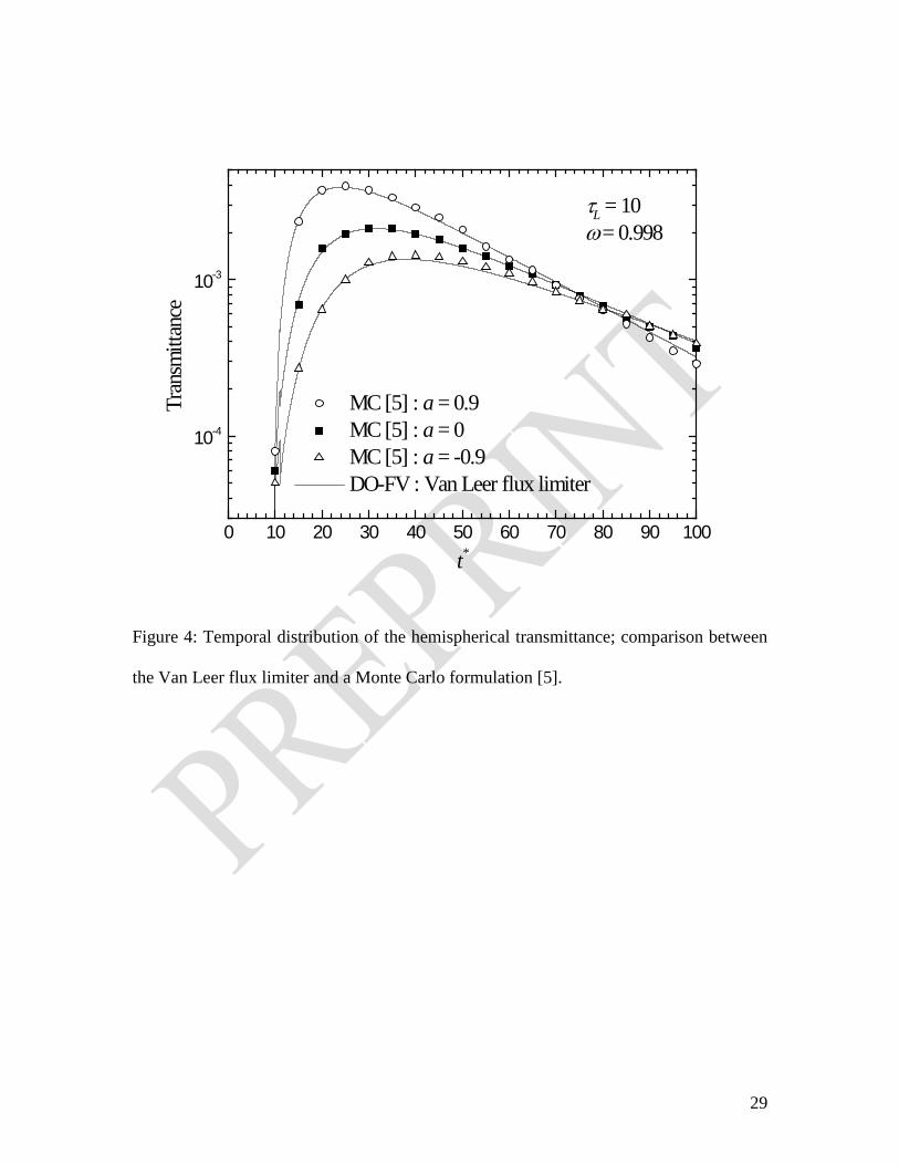
4.1. Problem 1: Optically thick and highly scattering medium

In this first problem, the optical thickness of the medium is τL = 10 while the scattering

albedo is ω = 0.998. The transmittance is calculated for three types of scattering media:

isotropic (a = 0), highly forward scattering (a = 0.9), and highly backward scattering (a =

-0.9). For this problem, 100 spatial nodes and 10 directions (equal weights polar

quadrature [22]) are sufficient to discretize the spatial and directional domains; no

significant improvement of the results has been observed beyond these thresholds. The

temporal discretization is determined by analyzing the Courant number defined in section

3.2; numerical simulations have been performed, and a Courant number of 0.2 has been

found to be optimal (results not presented).

Transmittances obtained from the DO-FV and the Van Leer flux limiters are

presented in figure 4, and compared with those obtained from a Monte Carlo (MC)

formulation for the same problem [5]. It is important to note that since the optical

thickness of the slab is 10, the minimal dimensionless time required by the radiation to

leave the medium is also 10.

17


The sharp diminution of transmittance at *t = 11, followed by an increase, is due

to fact that the collimated component of intensity has left the medium (square pulse of

dimensionless duration *pt = 1). A highly forward scattering medium (a = 0.9) leads to a

higher maximum of transmittance, since this phase function tends to throw the scattered

photons at the boundary τ = τL. On the other hand, a highly backward scattering phase

function (a = -0.9) produces longer travel paths of the scattered photons, leading to a

weaker maximum of transmittance. For a longer period of time, the transmittance is

higher for the backward scattering phase function (from t* ≈ 85) due to a more important

photons retention. Therefore, the transmittance vanishes more quickly when a = 0.9.

Figure 4 clearly indicates that for a large time scale (from 0 to 100), results

obtained with the Van Leer flux limiter are in good agreement with those obtained with a

reference Monte Carlo approach, even at early time periods. The same conclusion is

applicable for the Superbee flux limiter, as shown in figure 5.


In order to analyze more precisely the relative accuracy of flux limiters, the

transmittances are compared at early time periods with results obtained with a first order

exponential scheme [15]. Only results for a = 0.9 are shown, since early transmitted

radiation becomes more important as the medium is highly forward scattering.

18


Figure 6 shows that the radiative flux leaving the medium before the minimal

physical dimensionless travel time *Lt = 10 is considerably decreased with the flux

limiters. Generally, for all simulations carried out prior to this paper, the Superbee flux

limiter lead to more accurate results than the Van Leer. Despite this fact, early

transmitted radiation can not be completely avoided.

4.2. Problem 2: Medium of unit optical thickness and variable scattering albedo

In this second problem, the optical thickness of the medium is fixed at 1=Lτ while the

scattering albedo ω is variable (0.25, 0.50, 0.75 and 0.90). In all cases, the medium is

isotropically scattering (a = 0). This second test problem has been solved with a Discrete

Ordinates approach coupled with the Piecewise Parabolic Advection scheme (DO-PPA)

[8], which has been validated with a Monte Carlo formulation [5]. The same spatial,

angular, and temporal discretizations used for the first problem are found sufficient.

The transmittances, obtained from the DO-FV method coupled with the Van Leer

and Superbee flux limiters, are presented in figures 7 and 8, respectively. In this case, the

minimal dimensionless time needed by the radiation to leave the slab of unit optical

thickness is *Lt = 1.

19



The transmittance is more important as the scattering albedo increases. This can

be explained by the fact that a larger proportion of the pulsed collimated radiation beam

is scattered in the medium. Moreover, an increase of the scattering albedo leads to a

diminution of the mean free path of scattering, and hence to an increase of multiple

scattering, longer photons travel paths, and, consequently, a larger transmitted temporal

signal. Here again, the decrease of transmittance at t* = 2 is due to the fact that the

collimated component of radiation intensity has left the medium. After t* = 2, the

transmittance is only due to the diffuse part of radiation intensity.

It can be seen in figures 7 and 8 that the temporal distributions of transmittances

are, in general, in good agreement with those obtained from the DO-PPA. However, early

transmitted radiation can be observed on a temporal scale from 0 to 10, for both types of

flux limiters.

Figure 9 shows a comparison between transmittances obtained with the first order

exponential scheme [15] and flux limiters at early time periods for a scattering albedo of

ω = 0.9.


20

It is clear from figure 9 that the Superbee flux limiter leads to more accurate

results, even if there is still radiation transmitted before t* = 1.

5. CONCLUSION

The one-dimensional transient radiative transfer problem for absorbing and scattering

media has been solved in Cartesian coordinates using a Discrete Ordinates – Finite

Volume approach. The Van Leer and Superbee flux limiters, based on the second order

spatial scheme Lax-Wendroff, have been used in order to minimize the transmitted fluxes

emerging before the minimal time required by the radiation to leave the medium.

In general, results from the DO-FV coupled with flux limiters are in close

agreement with those from the literature. Moreover, a comparison at early time periods

with the transmittance obtained from a DO-FV and a first order exponential scheme has

shown that the flux limiters can substantially decrease the temporal numerical diffusion.

However, there is still a low transmitted flux before the minimal physical time required

by the radiation to leave the medium.

High order schemes coupled with flux limiters can not totally avoid this problem.

Indeed, a DO-FV formulation based in the space-time domain will never completely

prevent this problem due to the interdependence between the spatial and temporal

discretizations.

21

Therefore, second part of this work is devoted to the formulation, implementation,

and validation of a method for which the transient radiative transfer problem is solved in

the space-frequency domain.

ACKNOWLEDGMENTS

The author acknowledges Mathieu Francoeur (Radiative Transfer Laboratory, University

of Kentucky) and Rodolphe Vaillon (CETHIL, INSA de Lyon) for their collaboration

during these research works. The author is also grateful to Alan Wright (Invited

professor, UQAR-Lévis) and to the Natural Sciences and Engineering Research Council

of Canada (NSERC).

22

REFERENCES

[1] Rackmil, C.I. and Buckius, R.O., Numerical solution technique for the transient

equation of transfer. Numerical Heat Transfer, 1983, 6, 135-153.

[2] Kumar, S. and Mitra, K., Microscale aspects of thermal radiation transport and laser

applications. Advances in Heat Transfer, 1998, 33, 187-294.

[3] Boulanger, J. and Charette, A., Numerical developments for short-pulsed near infra-

red laser spectroscopy. Part II: inverse treatment. Journal of Quantitative Spectroscopy

and Radiative Transfer, 2005, 91, 297-318.

[4] Guo, Z., Kumar, S. and San, K.-C., Multidimensional monte carlo simulation of short-

pulse transport in scattering media. Journal of Thermophysics and Heat Transfer, 2000,

14(4), 504-511.

[5] Sawetprawichkul, A., Hsu, P.-F., Mitra, K. and Sakami, M., A monte carlo study of

transient radiative transfer within the one-dimensional multi-layered slab, in Proceedings

of the ASME, 2000, 366(1), 145-153.

[6] Wu, C.-Y. and Ou, N.-R., Differential approximations for transient radiative transfer

through a participating medium exposed to collimated irradiation. Journal of Quantitative

Spectroscopy and Radiative Transfer, 2002, 73, 111-120.

23

[7] Guo, Z. and Kumar, S., Radiation element method for transient hyperbolic radiative

transfer in plane-parallel inhomogeneous media. Numerical Heat Transfer part B, 2001,

39, 371-387.

[8] Sakami, M., Mitra, K. and Hsu, P.-F., Transient radiative transfer in anisotropically

scattering media using monotonicity-preserving schemes, in Proceedings of the ASME,

2000, 366(1), 135-143.

[9] Sakami, S., Mitra, K. and Hsu, P.-F., Analysis of light transport through two-

dimensional scattering and absorbing media. Journal of Quantitative Spectroscopy and

Radiative Transfer, 2002, 73, 169-179.

[10] Boulanger, J. and Charette, A., Numerical developments for short-pulsed near infra-

red laser spectroscopy. Part I: direct treatment. Journal of Quantitative Spectroscopy and

Radiative Transfer, 2005, 91, 189-209.

[11] Wu, S.-H. and Wu, C.-Y., Integral equation solution for transient radiative transfer

in nonhomogeneous anisotropically scattering media. Journal of Heat Transfer, 2000,

122, 818-822.

[12] Tan, Z.-M. and Hsu, P.-F., An integral formulation of transient radiative transfer.

Journal of Heat Transfer, 2001, 123, 466-475.

24

[13] Katika, K.M. and Pilon, L., Backward method of characteristics in radiative heat

transfer, in 4th International Symposium on Radiative Transfer, 2004.

[14] Katika, K.M. and Pilon, L., Ultra-short pulsed laser transport in a multilayered turbid

media, in Proceedings of IMECE, 2004, 1-9.

[15] Francoeur, M., Rousse, D.R. and Vaillon, R., Analyse du transfert radiatif

instationnaire en milieu semi-transparent absorbant et diffusant, in Compte-Rendus du VIe

Colloque Interuniversitaire Franco-Québécois, 2003, 08-07.

[16] Stone, J.M. and Mihalas, D., Upwind monotonic interpolation methods for the

solution of the time dependent radiative transfer equation. Journal of Computational

Physics, 1993, 100(2), 402-408.

[17] Ayranci, I. and Selçuk, N., MOL solution of DOM for transient radiative transfer in

3-D scattering media. Journal of Quantitative Spectroscopy and Radiative Transfer,

2004, 84, 409-422.

[18] Francoeur, M., Vaillon, R. and Rousse, D.R., Theoretical analysis of frequency and

time-domain methods for optical characterization of absorbing and scattering media.

Journal of Quantitative Spectroscopy and Radiative Transfer, 2005, 93, 139-150.

25

[19] Modest, M.F., Radiative Heat Transfer, 2nd edition, 2003 (Academic Press: San

Diego).

[20] Rousse, D.R., Numerical Predictions of Two-Dimensional Conduction, Convection,

and Radiation Heat Transfer. I – Formulation, Int. J. Thermal Sciences, 2000, 39, no. 3,

315-331.

[21] Leveque, R.J., Finite Volume Methods for Hyperbolic Problems, 2002 (University

Press: Cambridge).

[22] Colella, P. and Woodward, P.R., The piecewise parabolic method (PPM) for gas-

dynamical simulations. Journal of Computational Physics, 1984, 54, 174-204.

[23] Rousse, D.R., Numerical predictions of multidimensional conduction, convection

and radiation heat transfer in participating media, 1994, PhD thesis, McGill University.

26

FIGURES

0I

θ

µ

,z τcI

0τ = Lτ τ=,β ω

φ

0z = Lz z=

LL

ztc

=Lz

1

1L L

Lt tc

= >1L

2L2

2L L

Lt tc

= >

pt dI

nL

Figure 1: Schematic representation of the transient radiative transfer problem under

consideration.

27

jτ21−j 21+j

j

nmjI ,

nmjI ,

21+nm

jI ,21−

nmjI ,

1−nm

jI ,1+

1−j 1+j

µ

τ

0=τ

θ

Figure 2: Schematic representation of a pulsed collimated radiation beam propagating in

a participating medium.

28

−∆

+∆

j

1−j

1+j

21+j21−j

jτ∆

nmjI ,

1−

nmjI ,

nmjI ,

1+

τ

Figure 3: Representation of a control volume and its surrounding nodes.

29

0 10 20 30 40 50 60 70 80 90 100

10-4

10-3

τL = 10ω = 0.998

MC [5] : a = 0.9 MC [5] : a = 0 MC [5] : a = -0.9 DO-FV : Van Leer flux limiter

Tran

smitt

ance

t*

Figure 4: Temporal distribution of the hemispherical transmittance; comparison between

the Van Leer flux limiter and a Monte Carlo formulation [5].

30

0 10 20 30 40 50 60 70 80 90 100

10-4

10-3

τL = 10ω = 0.998

MC [5] : a = 0.9 MC [5] : a = 0 MC [5] : a = -0.9 DO-FV : Superbee flux limiter

Tran

smitt

ance

t*


the Superbee flux limiter and a Monte Carlo formulation [5].

31

8,0 8,5 9,0 9,5 10,0 10,5 11,0 11,5 12,010-5

10-4

10-3

τL = 10ω = 0.998a = 0.9

DO-FV : Exponential scheme [15] DO-FV : Van Leer flux limiter DO-FV : Superbee flux limiter

Tr

ansm

ittan

ce

t*


the Van Leer and Superbee flux limiters and the exponential interpolation scheme at early

time periods.

32

0 1 2 3 4 5 6 7 8 9 1010-4

10-3

10-2

10-1

100

τL = 1a = 0

DO-PPA [8] : ω = 0.25 DO-PPA [8] : ω = 0.50 DO-PPA [8] : ω = 0.75 DO-PPA [8] : ω = 0.90 DO-FV : Van Leer flux limiter

Tran

smitt

ance

t*


the Van Leer flux limiter and the DO-PPA method [8].

33

0 1 2 3 4 5 6 7 8 9 1010-4

10-3

10-2

10-1

100

τL = 1a = 0

DO-PPA [8] : ω = 0.25 DO-PPA [8] : ω = 0.50 DO-PPA [8] : ω = 0.75 DO-PPA [8] : ω = 0.90 DO-FV : Superbee flux limiter

Tr

ansm

ittan

ce

t*


the Superbee flux limiter and the DO-PPA method [8].

34

0,5 0,6 0,7 0,8 0,9 1,0 1,1 1,2 1,3 1,4 1,510-4

10-3

10-2

10-1

100

τL = 1ω = 0.9a = 0 DO-FV : Superbee

flux limiter DO-FV : Van Leer

flux limiter DO-FV : Exponential

scheme [15]

Tr

ansm

ittan

ce

t*


the Van Leer and Superbee flux limiters and the exponential interpolation scheme at early

time periods.

numerical predictions of short-pulsed laser transport … laser transport in absorbing and...

Documents