Mathematical and Computer Modelling 50 (2009) 653–664

Contents lists available at ScienceDirect

Mathematical and Computer Modelling

journal homepage: www.elsevier.com/locate/mcm

Numerical schemes for a size-structured cell population model withequal fissionL.M. Abia, O. Angulo ∗, J.C. López-Marcos, M.A. López-MarcosDepartamento de Matemática Aplicada, Universidad de Valladolid, Valladolid, Spain

a r t i c l e i n f o

Article history:Received 19 September 2008Accepted 12 December 2008

Keywords:Cell population modelSize-structured populationNumerical simulationConvergence analysisStable size distribution

a b s t r a c t

We study numerically the evolution of a size-structured cell population model, with finitemaximum individual size and minimum size for mitosis. We formulate two schemes forthe numerical solution of such a model. The schemes are analysed and optimal rates ofconvergence are derived. Some numerical experiments are also reported to demonstratethe predicted accuracy of the schemes.We also consider the behaviour of themethodswithrespect to the different discontinuities that appear in the solution to the problem and thestable size distribution. In addition, the numerical schemes are used to study asynchronousexponential growth.

© 2009 Elsevier Ltd. All rights reserved.

1. Introduction

Structuredpopulationmodels describe the evolution of a population bymeans of the individuals’ vital properties (growth,division, mortality, fertility, etc.) which depend on individual physiological characteristics (structuring variables such as ageor size). In this work, we analyse the evolution over time of the density of a size-structured cell population described by alinear size-structured model. In the study of cell-population dynamics, linear structured models were first introduced byBell and Anderson [1,2] and Fredrickson et al. [3] (this work was motivated by the study of the growth of a procaryotic cellpopulation). Sinko and Streifer [4] also presented a nonlinear model based on reproduction by fission. However, the linearmodels maintained their interest due to the existence of the stable-type size distribution property and the asynchronousexponential growth, which show the behaviour of the growth of cells in an in vitro culture. The existence of a stable sizedistribution property in some cases was studied by Diekmann et al. [5] in a variant of the Bell–Anderson [1,2] model for size-structured cell population growth (reproduction occurs by fission into two equal parts). We refer to the books by Metz andDiekmann [6], Lasota andMackey [7,8] and Perthame [9] to illustrate the principal mathematical problems to be solved andthe main tools to be used in this context. The study of cell distribution is also taken into account in a cell dwarfism modelconsidered in [10] and in a recent paper [11] in which an inverse problem for an integro–differential equation is given toobtain the division rate from the measured stable size distribution of the population.We shall here concentrate on the size-structured cell population model proposed by Diekmann et al. [5]. In this model,

the reproduction is given by the fission of the cell in two equal parts (mitosis). The model also assumes that cells divideafter they have reached aminimal size a > 0. Therefore, there exists a minimum size whose value is a2 . Moreover, cells haveto divide before they reach a maximal size, which is normalized to be x = 1. It is also supposed that the environment isunlimited and all possible nonlinear mechanisms are ignored. The model is given by a conservation law,

ut(x, t)+ (g(x) u(x, t))x = −µ(x) u(x, t)− b(x) u(x, t)+ 4 b(2 x) u(2 x, t), (1.1)

∗ Corresponding address: Departamento de Matemática Aplicada, Escuela Universitaria Politécnica, Universidad de Valladolid, C/ Fco. Mendizabal, 1,47014 Valladolid, Spain. Tel.: +34 983 423000x6805; fax: +34 983 423490.E-mail addresses: abia@mac.cie.uva.es (L.M. Abia), oscar@mat.uva.es (O. Angulo), lopezmar@mac.uva.es (J.C. López-Marcos), malm@mac.uva.es

(M.A. López-Marcos).

0895-7177/$ – see front matter© 2009 Elsevier Ltd. All rights reserved.doi:10.1016/j.mcm.2009.05.023

654 L.M. Abia et al. / Mathematical and Computer Modelling 50 (2009) 653–664

a2 < x < 1, t > 0, a boundary condition,

u( a2, t)= 0, t > 0, (1.2)

and an initial size distribution,

u(x, 0) = ϕ(x),a2≤ x ≤ 1. (1.3)

The independent variables x and t represent size and time, respectively. The dependent variable u(x, t) is the size-specificdensity of cells with size x at time t , and we assume that the size of any individual varies according to the following ordinarydifferential equation:

dxdt= g(x). (1.4)

The nonnegative functions g ,µ and b represent the growth,mortality and division rate, respectively. These are usually calledthe vital functions and define the life history of the individuals. Note that all of them depend on the size x (the internalstructuring variable). We should point out that, in (1.1), the reproduction process into two equal parts has been consideredin the two terms in which the division rate appears. Here, we have to note that the term 4 b(2 x) u(2 x, t) is interpreted aszero whenever x > 1

2 . The condition (1.2) reflects that cells with a size less thana2 cannot exist; this is a consequence of the

fact that cells only divide after the minimal size a > 0.In accordance with accepted biological wisdom, there exists a maximum size [24]. This means that cells will divide or

die with probability one before reaching it. Thus, if we consider the survival property, i.e. the probability that an individualof size x0 reaches size x,

Π(x) = exp(−

∫ x

x0

µ(s)+ b(s)g(s)

ds),a2≤ x0 <

12,

the hypothesis of considering a maximum size implies that limx→1− Π(x) = 0. One of the forms in which this fact could bereflected consists in taking into account the growth functions introduced by Von Bertalanffy [12]. This kind of functionssatisfies

∫ 1x0

dsg(s) = ∞, which is enough to verify the required condition whenever µ and b are positive and bounded

functions. Biologically it means that cells die or divide before they reach the maximum size. Note that if g is a continuousfunction defined on

[ a2 , 1

]then this hypothesis implies that g(1) = 0. Moreover, the solution of the problem must satisfy

u(1, t) = 0, t > 0, because we suppose that initially there are no cells of maximum size [13].On the other hand, the smoothness of the solution of the problem depends on the smoothness properties of the vital

functions and the initial condition. It is also important to consider the compatibility between the initial and the boundaryconditions which impose restrictions on the initial value of the solution at the minimum size. The solution and/or some ofthe derivativeswould have discontinuities at the corresponding point of the characteristic curve that begins at x = a

2 , if someof the compatibility conditions are not satisfied. One of these is ϕ(0) = 0, which implies the logic continuity property of thesolution. Moreover, we consider that the solution vanishes out of the domain (see Cushing [13]). The solution would be zeroat the maximum size in order to be continuous. However, the properties of the product b u could provoke a discontinuityat the maximum size. This would introduce a discontinuity in the second derivative of the solution at x = 1

2 and at thecorresponding locus at the characteristic curve that begins at that point. Therefore, the solution would be only continuouslydifferentiable.From a numerical point of view, the integration of cell models has been studied in recent years. In the following, we will

introduce the studies in which numerical schemes are proposed in order to solve size-structured cell population models.We discuss the problems in which the domain of the spatial variable could be both finite and infinite. The first proposalswere developed in order to solve the problem in which the maximum size was not considered. The work carried out by Liouet al. [14] presents a theoretical approach based on a successive generations technique. Later,Mantzaris et al. [15] proposed afinite difference scheme to solve the problem and Angulo and López-Marcos [16] introduced a characteristic curves schemeand completed the first convergence analysis made within this framework. The maximum size of the cell is a biologicalwisdomwhichmakes these models unrealistic. These models also avoid treatment of the discontinuities caused by it. Otherauthors considered models in which the finite interval case is considered. Mantzaris et al. [17–19] proposed numericalschemes of high order based on finite differences, spectral and finite element methods, respectively. These authors showthe efficiency of each scheme. However, they do not pay attention to either the compatibility of the initial and boundaryconditions or the discontinuities caused by the maximum size. The problem of the maximum size is not considered withinthe test problems that the authors proposed. They do not demonstrate the convergence of the numerical schemes presented.Moreover, the lack of smoothness properties of the solution would negatively affect the efficiency of such higher ordermethods.The paper is organized as follows. In Section 2, we introduce the numerical schemes employed: a method based on an

upwind discretization and a scheme based on a representation of the solution along the characteristic curves which aredescribed in detail. Section 3 is entirely devoted to the convergence analysis for both methods. We believe that they arethe first convergence analyses for schemes applied to the problem (1.1)–(1.3). In Section 4, we introduce the numericalexperimentation. We present two different test problems: one of them satisfies three compatibility conditions and the

L.M. Abia et al. / Mathematical and Computer Modelling 50 (2009) 653–664 655

other only satisfies the continuity one, which introduces a discontinuity in the first derivative at the characteristic curve thatbegins at the minimum size. We show the convergence of both schemes and their efficiency with a plot (CPU time versusglobal errors on a logarithmic scale). We also validate our numerical simulation with comparisons related to the stable sizedistribution and we compare the behaviour of both schemes with respect to the discontinuities of the derivatives.

2. Numerical methods

We will now introduce two new numerical schemes of first order which adapt the peculiarities of the cell populationmodel. We will not employ higher order methods due to the fact that the solution is only first order continuously differen-tiable and they would increase the computational cost and the algorithm complexity without any guarantee of obtaining abetter solution.The first one is a finite difference method based on an upwind technique following the direction of the characteristic

curves. The size discretization is built in order that if x is a grid point then 2 x is also. Below, we describe the numericalscheme.Let J be a positive integer. We introduce the grid points xj = a

2 + j h, 0 ≤ j ≤ J + J∗, where h = a

2 J is the mesh size; thismeans that xJ = a, and J∗ =

[ 1−ah

]. The step length in time is denoted by k, and tn = n k, 0 ≤ n ≤ N , N = [T/k], are the

discrete time levels. We also define r = kh . The subscript j refers to the grid point xj and the superscript n to the time level tn.

If Unj are the numerical approximations to the values u(xj, tn), 0 ≤ j ≤ J + J∗, 0 ≤ n ≤ N , the scheme can be obtained by

discretizing the derivatives in (1.1) in the following way:

Un+1j − Unjk

+gj Unj − gj−1 U

nj−1

h= −(µj + bj)Un+1j + 4 bJ+2 j UnJ+2 j, (2.1)

j = 1, 2, . . . , J + J∗, where gj = g(xj), µj = µ(xj), bj = b(xj), 0 ≤ j ≤ J + J∗, and

bj Unj ={bj Unj , j ≤ J + J∗,0, j > J + J∗.

In addition, we set Un0 = 0, 0 ≤ n ≤ N due to the boundary condition (1.2). The implicit formula in (2.1) can be easilytransformed into the following explicit one:

Un+1j =Unj − r

(gj Unj − gj−1 U

nj−1

)+ 4 k bJ+2 j UnJ+2 j

1+ k (µj + bj), (2.2)

j = 1, 2, . . . , J + J∗.The second approach is a numericalmethodwhich integrates the problem along the characteristic curves. It also employs

a theoretical representation of the solution. Now, we introduce the theoretical framework of this method.We begin by rewriting the partial differential equation. If we define µ∗(x) = g ′(x) + µ(x) + b(x), then (1.1) can be

transformed intout(x, t)+ g(x) ux(x, t) = −µ∗(x) u(x, t)+ 4 b(2 x) u(2 x, t), (2.3)

a2 < x < 1, t > 0. The model is completed with the initial condition (1.3) and the boundary condition (1.2).Now, we denote the characteristic curve of the Eq. (1.1) which takes the value x∗ at the time instant t∗ by x(t; t∗, x∗). This

characteristic curve is the solution of the following initial value problem:{ ddtx(t; t∗, x∗) = g(x(t; t∗, x∗)), t > t∗,

x(t∗; t∗, x∗) = x∗.(2.4)

Then, we define the functionw(t; t∗, x∗) = u(x(t; t∗, x∗), t), t ≥ t∗, (2.5)

which satisfies the following initial value problem:{ ddtw(t; t∗, x∗) = −µ∗ (x (t; t∗, x∗)) w(t; t∗, x∗)+ 4 b(2 x (t; t∗, x∗)) u(2 x (t; t∗, x∗) , t), t ≥ t∗,

w(t∗; t∗, x∗) = u(x∗, t∗),(2.6)

and whose solution has the following representation formula:

w(t; t∗, x∗) = u(x∗, t∗) exp{−

∫ t

t∗µ∗ (x (τ ; t∗, x∗)) dτ

}+

∫ t

t∗exp

{−

∫ t

τ

µ∗ (x (s; t∗, x∗)) ds}

× 4 b(2 x (τ ; t∗, x∗)) u(2 x (τ ; t∗, x∗) , τ )dτ , t ≥ t∗. (2.7)Therefore, the partial differential equation (2.3) is reduced to a family of differential equations. Note thatwehave to integratetwo types of problem: an equation that defines the characteristic curves (2.4) and another that obtains the solution of theproblem (2.6) through (2.7). We also have to take into account that, in these last two equations, we have again considereda term which is zero when the structuring variable is greater than 12 .

656 L.M. Abia et al. / Mathematical and Computer Modelling 50 (2009) 653–664

Below, we will describe the characteristic curves scheme. Given a positive integer N , we define k = T/N and introducethe discrete time levels tn = n k, 0 ≤ n ≤ N . Next, we obtain a grid on the space variable which is nonuniform and invariantwith time, due to the fact that the growth rate depends only on x. It is usually called the natural grid, as considered in [20,21],

a2= x0 < x1 < · · · < xJĎ < xJĎ+1 = 1, (2.8)

such that the points (xj, tn) and (xj+1, tn+1), 0 ≤ j ≤ JĎ − 1, 0 ≤ n ≤ N − 1, belong to the same characteristic curve. Ingeneral, this is not possible because we are unable to solve (2.4) in an analytical way, so we integrate (2.4) numerically bymeans of the modified Euler method,

x0 =a2,

xj+1 = xj + k g(xj +

k2g(xj)

), 0 ≤ j ≤ JĎ − 1.

Now, in actuality, the points (xj, tn) and (xj+1, tn+1), 0 ≤ j ≤ JĎ, 0 ≤ n ≤ N − 1, are not necessarily on the same character-istic curve. In addition, Angulo et al. [21] established the conditions on which we can choose positive constants K0 and K1,independent of h, such that

K0 h ≤ 1− xJĎ ≤ K1 h,

for sufficiently small h, property that is required in the analysis. We refer to [21] for further details.Next, we refer to the grid point xj by a subscript j and to the time level tn by a superscript n, and we define unj = u(xj, tn),

0 ≤ j ≤ JĎ + 1, 0 ≤ n ≤ N . Let Unj be a numerical approximation to unj , 0 ≤ j ≤ JĎ + 1, 0 ≤ n ≤ N − 1. The next stage in

our method is to obtain an approximation Un+1j+1 to un+1j+1 for 0 ≤ j ≤ JĎ − 1, 0 ≤ n ≤ N − 1.

Un+1j+1 = Unj exp

{−kµ∗

(xj)}+ 4 k exp

{−kµ∗

(xj)}¯b2·j ¯U

n

2·j, (2.9)

where, if we consider xn as the corresponding approximation at tn of the characteristic curve which begins at x = a2 ,¯b2·j ¯U

n

2·jis defined by means of the following interpolation technique because, in general, 2 xj does not belong to the spatial grid:

¯b2·j ¯Un

2·j =

{b(2 xj)UnM−1, xM−1 ≤ 2 xj < xM ≤ 1, xM ≤ xn,b(2 xj)UnM , xM−1 ≤ 2 xj < xM ≤ 1, xM > xn,0, 2 xj ≥ 1.

Therefore,we define it depending onwhich side of xnwe find xM . In this definition,we have taken into account twoproblems.First, the solution of (2.3) is zero out of the interval

[ a2 , 1

]and second, the initial and the boundary conditions may not be

compatible. We also have to consider Un+1JĎ+1 = 0, 0 ≤ n ≤ N − 1, because x = xJĎ+1 is a characteristic curve and there areno cells with the maximum size.

3. Convergence analysis

In this section, we carry out the convergence analysis of both schemes. We know that there is a discontinuity at x = 12

on all the second derivatives; therefore we only suppose that u is the solution of the problem (1.1)–(1.3), and has Lipschitzcontinuous first derivatives in [ a2 , 1]. Fromnowon,C will denote a positive constantwhich is independent of k,n (0 ≤ n ≤ N)and j (0 ≤ j ≤ J); C possibly has different values in different places.

3.1. Upwind method

Below, we complete the convergence proof of the upwind basedmethod. First, we study the consistency of the proposednumerical method. We define

unj = u(xj, tn), 0 ≤ j ≤ J + J∗, unj ={unj , j < J + J∗,0, j ≥ J + J∗, (3.1)

0 ≤ n ≤ N and the local discretization error,

τ n+1j =un+1j − u

nj

k+gj unj − gj−1 u

nj−1

h+ (µj + bj) un+1j − 4 bJ+2 j u

nJ+2 j, (3.2)

1 ≤ j ≤ J + J∗, 0 ≤ n ≤ N − 1.

Lemma 1. Let functions µ, b, g be C1([ a2 , 1]) and let u have Lipschitz continuous first derivatives in [a2 , 1]. Then, as k→ 0, the

following estimates hold:

|τ n+1j | = O(k+ h), 1 ≤ j ≤ J + J∗, 0 ≤ n ≤ N − 1. (3.3)

L.M. Abia et al. / Mathematical and Computer Modelling 50 (2009) 653–664 657

Proof. If we take into account that the data functions are sufficiently smooth, we obtain

τ n+1j = (ut)nj + ((g u)x)nj + (µj + bj) u

nj − 4 bJ+2 j u

nJ+2 j +

∫ 1

0

(ut(xj, tn + s k)− ut(xj, tn)

)ds

+

∫ 1

0

((g u)x(xj + σ h, tn)− (g u)x(xj, tn)

)dσ + k (µj + bj) ut(xj, tn + ε k), ε ∈ (0, 1), (3.4)

1 ≤ j ≤ J + J∗, 0 ≤ n ≤ N − 1. Then, as ut and (g u)x are Lipschitz continuous, we have

|τ n+1j | ≤ C (h+ k), (3.5)

1 ≤ j ≤ J + J∗, 0 ≤ n ≤ N − 1. And the estimates hold. �

Now, we define

en = (en0, . . . , enJ+J∗), enj = u

nj − U

nj , 0 ≤ j ≤ J + J∗,

0 ≤ n ≤ N , where unj are the nodal values of the theoretical solution and Unj are the numerical approximations obtained by

means of our numerical method, and

enj ={enj , j < J + J∗,0, j ≥ J + J∗,

0 ≤ n ≤ N . Also,

‖p‖∞ = max0≤j≤J+J∗

{|pj|}, p = (p0, p1, . . . , pJ+J∗).

In the following, we prove the convergence of the numerical scheme.

Theorem 2. Under the hypotheses of Lemma 1, if ‖e0‖∞ = O(k), as k→ 0, where r is a fixed constant that satisfies r ‖g‖∞ < 1,then

‖en‖∞ ≤ C k, 0 ≤ n ≤ N. (3.6)

Proof. From Eqs. (2.2) and (3.2) we obtain

en+1j =

(1− r gj

)enj + r gj−1 e

nj−1 + 4 k bJ+2 j e

nJ+2 j + k τ

n+1j

1+ k (µj + bj), (3.7)

1 ≤ j ≤ J + J∗, 0 ≤ n ≤ N − 1. Due to the properties of the functions data

|en+1j | ≤ (1+ C k) ‖en‖∞ + 4 k bJ+2 j ‖en‖∞ + k ‖τn+1‖∞, (3.8)

1 ≤ j ≤ J + J∗, 0 ≤ n ≤ N − 1. Then, by means of a recursive argument, we arrive at

‖en‖∞ ≤ (1+ C k)n ‖e0‖∞ + kn∑l=0

(1+ r k)n−l ‖τ l‖∞, (3.9)

1 ≤ n ≤ N , and by means of (3.3), we have

‖en‖∞ ≤ eC T ‖e0‖∞ + C k, 1 ≤ n ≤ N. � (3.10)

3.2. Characteristics scheme

Next, we study the consistency of the method that integrates along the characteristic curves using a representation ofthe solution. We define

unj = u(xj, tn), ¯un2·j =

{unM−1, xM−1 ≤ 2 xj < xM ≤ 1, xM ≤ xn,unM , xM−1 ≤ 2 xj < xM ≤ 1, xM > xn,0, 2 xj ≥ 1,

(3.11)

0 ≤ j ≤ JĎ + 1, 0 ≤ n ≤ N , where xn is the corresponding approximation at tn of the characteristic curve which begins atx = a

2 , 0 ≤ n ≤ N . And the local discretization error,

τ n+1j+1 =1k

(un+1j+1 − u

nj exp

{−kµ∗

(xj)}+ 4 k exp

{−kµ∗

(xj)}¯b2·j ¯u

n2·j

), (3.12)

0 ≤ j ≤ JĎ − 1, 0 ≤ n ≤ N − 1.

658 L.M. Abia et al. / Mathematical and Computer Modelling 50 (2009) 653–664

Lemma 3. Let g be two times continuously differentiable and functionsµ∗, b and u be continuously differentiable. Then, as k→ 0,the following estimates hold:

|τ n+1j+1 | = O(k), 0 ≤ j ≤ JĎ, 0 ≤ n ≤ N − 1. (3.13)

Proof. If we take into account the convergence properties of the rectangular quadrature rule, the modified Euler method,the extrapolation procedure and that the function g is C2, and that the functionsµ∗, b and u are continuously differentiable,we obtain

|τ n+1j+1 | ≤1k

∣∣un+1j+1 − u (x (tn+1; xj, tn) , tn+1)∣∣+1k

∣∣unj ∣∣ ∣∣∣∣exp{− ∫ tn+1

tnµ∗(x(τ ; tn, xj

))dτ}− exp

{−kµ∗

(xj)}∣∣∣∣

+4k

∣∣∣∣∫ tn+1

tnexp

{−

∫ tn+1

τ

µ∗(x(s; tn, xj

))ds}b(2 x

(τ ; tn, xj

)) u(2 x

(τ ; tn, xj

), τ )dτ

−

∫ tn+1

tnexp

{−(tn+1 − τ) µ∗

(x(τ ; tn, xj

))}b(2 x

(τ ; tn, xj

)) u(2 x

(τ ; tn, xj

), τ )dτ

∣∣∣∣+4k

∣∣∣∣∫ tn+1

tnexp

{−(tn+1 − τ) µ∗

(x(τ ; tn, xj

))}b(2 x

(τ ; tn, xj

)) u(2 x

(τ ; tn, xj

), τ )dτ

− k exp{−kµ∗

(xj)}b(2 xj) u(2 xj, tn),

∣∣∣∣+ 4 exp {−kµ∗ (xj)} b(2 xj) ∣∣∣u(2 xj, tn)− ¯un2·j∣∣∣≤ C k,

0 ≤ j ≤ JĎ − 1, 0 ≤ n ≤ N − 1. And the estimates hold. �

In the following result, we prove the convergence of the numerical method. We defineen = (en0, . . . , e

nJĎ , e

nJĎ+1), enj = u

nj − U

nj , 0 ≤ j ≤ JĎ + 1,

0 ≤ n ≤ N , where unj are the nodal values of the theoretical solution and Unj are the numerical approximations obtained by

means of our numerical method. And

¯en2·j =

{enM−1, xM−1 ≤ 2 xj < xM ≤ 1, xM ≤ xn,enM , xM−1 ≤ 2 xj < xM ≤ 1, xM > xn,0, 2 xj ≥ 1,

0 ≤ j ≤ JĎ + 1, (3.14)

0 ≤ n ≤ N , where xn is, again, the corresponding approximation at tn of the characteristic curve which begins at x = a2 ,

0 ≤ n ≤ N .

Theorem 4. Under the hypotheses of Lemma 3, if ‖e0‖∞ = O(k), as k→ 0, then

‖en‖∞ ≤ C k, 0 ≤ n ≤ N. (3.15)

Proof. From Eqs. (2.9) and (3.12), we have

en+1j+1 = enj exp

{−kµ∗

(xj)}+ 4 k exp

{−kµ∗

(xj)}¯b2·j ¯e

n2·j + k τ

n+1j+1 , (3.16)

0 ≤ j ≤ JĎ − 1, 0 ≤ n ≤ N − 1. Then, taking into account the smoothness properties of the functions µ∗ and b, we arrive at

|en+1j+1 | ≤ (1+ C k) |enj | + C k ‖e

n‖∞ + k |τ n+1j+1 |, (3.17)

0 ≤ j ≤ JĎ − 1, 0 ≤ n ≤ N − 1, and

|en+1j+1 | ≤ (1+ C k) ‖en‖∞ + k ‖τn+1‖∞, (3.18)

0 ≤ j ≤ JĎ − 1, 0 ≤ n ≤ N − 1. Then, by means of a recursive argument, we obtain

|enj | ≤ (1+ C k)n‖e0‖∞ + k

n∑l=1

(1+ C k)n−l ‖τ l‖∞, (3.19)

1 ≤ j ≤ JĎ, 0 ≤ n ≤ N − 1. And, using (3.13), we arrive at

‖en‖∞ ≤ eC T ‖e0‖∞ + C k, (3.20)

1 ≤ n ≤ N , and the estimative holds. �

L.M. Abia et al. / Mathematical and Computer Modelling 50 (2009) 653–664 659

Table 1Test Problem 1. Results for the upwind scheme. Upper number: error; left-lower number: CPU time (in seconds), right-lower number: numericalconvergence order.

k h1.25e−2 6.25e−3 3.125e−3 1.563e−3 7.813e−4 3.906e−4

1.111e−1 2.192e−20.811

5.556e−2 2.348e−2 1.459e−21.613 3.224 0.587

2.778e−2 2.417e−2 1.614e−2 8.812e−33.294 6.530 0.541 13.16 0.727

1.389e−2 2.449e−2 1.683e−2 1.002e−2 4.781e−36.379 12.89 0.521 26.09 0.688 52.23 0.882

6.944e−3 2.465e−2 1.717e−2 1.058e−2 5.598e−3 2.256e−312.97 25.80 0.513 52.99 0.670 111.1 0.840 214.3 1.08

3.472e−3 2.472e−2 1.733e−2 1.085e−2 5.989e−3 2.752e−3 7.959e−426.04 52.35 0.508 105.2 0.662 211.7 0.821 422.4 1.02 845.4 1.50

Remark. Both methods give positive solutions, although we have not presented their proof due to their simplicity.

4. Numerical results

We have carried out an exhaustive numerical experimentation with the schemes defined in Section 2. We haveconsidered different test problems but, in this work, we present the results obtained with two of them. The numericalintegration for each numerical experiment was carried out on the time interval [0, 10].

Test Problem 1. Weemploy an initial conditionwhich satisfies three compatibility conditions and a division functionwhichis continuously differentiable. We consider the minimum size at which a cell divides as a = 1

4 . We choose the size-specificgrowth rate as g(x) = 0.1 (1− x) and the size-specific division rate function as

b(x) =

0, x ∈

[ a2, a],

g(x)φb(x)

1−∫ xa φb(s) ds

, x ∈ [a, 1] ,

0, x > 1,

where we have considered that each cell has a stochastically predetermined size at which fission has to occur, which is givenby a probability density φb [6]. In this case it is given by

φb(x) =

160117

(−23+83x)3, x ∈

[a,a+ 12

],

32117

(−20+ 40 x+

3203

(x−

58

)2+51209

(x−

58

)3 (83x−

113

)), x ∈

(a+ 12

, 1].

We consider that the mortality rate is µ(x) = 0. Finally, we take the initial condition as ϕ(x) = (1 − x)(x− a

2

)3. As wepointed out, the initial and boundary conditions satisfy three compatibility conditions because ϕ( a2 ) = ϕ

′( a2 ) = ϕ′′( a2 ) = 0.

Thus, the only discontinuity is caused by the maximum size at x = 12 and at the characteristic curve which begins at this

point.

Test Problem 2. In this case only one compatibility condition is satisfied. Then, new discontinuities appear in the first andsecond derivatives which propagate along the characteristic that begins at x = a

2 . We use the same vital functions as in TestProblem 1, but the initial condition is given by

ϕ(x) = (1− x)(x−

a2

),

which only satisfies ϕ( a2 ) = 0, the first compatibility condition.

Since we do not know the analytical solutions of both problems, in order to estimate experimentally the order ofconvergence (and to verify the theoretical results), we build error tableaux where we take as the theoretical solution thenumerical approximation obtained with k∗ = 1.736111e−3 and h∗ = 1.953125e−4, in the case of the upwind basedscheme and k∗ = 7.8125e−3 for the characteristics scheme. In addition, we can compare their computational efficiency.In Tables 1 and 2, we present the results obtained for the first test problem with the upwind scheme and the

characteristics method, respectively. Tables 3 and 4 show the results for the second test problem. In each entry of columns

660 L.M. Abia et al. / Mathematical and Computer Modelling 50 (2009) 653–664

Table 2Test Problem 1. Results for the characteristics method. Error, numerical convergence order and CPU time (in seconds).

k Error Order CPU time

1 4.688e−2 0.0305e−1 3.815e−2 0.297 0.1402.5e−1 2.560e−2 0.576 0.6611.25e−1 1.528e−2 0.744 2.9846.25e−2 8.318e−3 0.878 13.623.125e−2 4.353e−3 0.934 61.421.563e−2 2.226e−3 0.967 273.9

Table 3Test Problem 2. Results for the upwind scheme. Upper number: error; left-lower number: CPU time (in seconds), right-lower number: numericalconvergence order.

k h1.25e−2 6.25e−3 3.125e−3 1.563e−3 7.813e−4 3.906e−4

1.111e−1 6.597e−20.831

5.556e−2 7.278e−2 4.387e−21.663 3.244 0.588

2.778e−2 7.551e−2 5.013e−2 2.836e−23.224 6.500 0.538 13.08 0.629

1.389e−2 7.676e−2 5.271e−2 3.349e−2 1.733e−26.449 13.05 0.519 26.33 0.582 52.69 0.711

6.944e−3 7.735e−2 5.390e−2 3.567e−2 2.135e−2 9.481e−312.92 26.26 0.510 52.51 0.564 105.5 0.650 211.1 0.870

3.472e−3 7.764e−2 5.446e−2 3.669e−2 2.308e−2 1.252e−2 3.924e−326.01 52.18 0.506 105.2 0.555 210.5 0.628 421.1 0.770 843.9 1.27

Table 4Test Problem 2. Results for the characteristics method. Error, numerical convergence order and CPU time (in seconds).

k Error Order CPU time

1e−0 1.008e−1 0.04115e−1 6.385e−2 0.659 0.1302.5e−1 3.779e−2 0.757 0.6411.25e−1 2.124e−2 0.831 2.9646.25e−2 1.121e−2 0.923 13.583.125e−2 5.774e−3 0.957 61.181.5625e−2 2.930e−3 0.979 273.2

two to seven of Tables 1 and 3, the upper value represents the global error for the upwind based method,

ek,h = ‖UNk,h − UNk∗,h∗‖∞,

where k and h are the discretization parameters that we employed in the corresponding numerical experiment and themaximum norm only takes into account the values on the coarsest grid. The lower number on the left is the CPU timemeasured in seconds and the lower number on the right is the order s of the method as computed from

s =log(e2 k,2 h/ek,h)

log(2).

In Tables 2 and 4, the second column shows the global error for the characteristics scheme,

ek = ‖UNk − UNk∗‖∞,

where k is the discretization parameter that we employed in the corresponding numerical experiment and, again, themaximum norm only takes into account the values on the coarsest natural grid. In the third column, the order s is computedas

s =log(e2 k/ek)log(2)

.

Finally, the fourth column shows the CPU time measured in seconds.Each row (and each column) of the tables corresponds to a different value of the time (and spatial) discretization

parameters, respectively. The values in Tables 1 and 3 allow us to comment that the upwind based method is not ableto obtain the solution of the problem when the CFL condition (Courant–Friedrichs–Lewy condition) is not satisfied. Thissituation is shown in Theorem 2, where the condition r ‖g‖∞ < 1 is needed for the convergence of the method. The results

L.M. Abia et al. / Mathematical and Computer Modelling 50 (2009) 653–664 661

100

101

102

103

10–4

10–3

10–2

10–1

cpu time

erro

r

Upwind MethodCharacteristic Method

Fig. 1. Efficiency plot for Test Problem 1. Characteristic method (*) and upwind method (+).

in Tables 1 and 2 clearly confirm the expected first order of convergence for bothmethods. On the other hand, when the lackof compatibility appears (for the second test problem) Table 3 shows how the upwind based method loses the convergenceorder and the results in Table 4 confirm that the characteristics scheme keeps the order of convergence.In Fig. 1, we show an efficiency plot in logarithmic scale (corresponding to the first test problem) where we present the

error (in the vertical axis) and the work, measured as the CPU time spent in seconds (in the horizontal axis). We present theresults obtained when the ratio employed (r = k

h = 8.889) is the most efficient for the upwind method among the valuespresented in the Table. The characteristics based method is also more efficient than the upwind scheme for the second testproblem.Our numerical schemes can be used to study the stable size distribution, u(x). It can be computed by taking into account

that

u(x, t) ≈ C eσ t u(x),∫ 1

a/2u(x) dx = 1,

where σ is the Malthusian parameter (intrinsic rate of natural increase). Both u(x) and σ do not depend on the initialcondition and only the constant C depends on the initial condition. References [22,23] treat the stable size distributionfor age-structured models. In the case of size-structured models, the work of Diekmann [5] proved the existence of a stablesize distribution if g(2 x) < 2 g(x). From our numerical approximations to the density of the population, we can computean approximation to the stable size distribution because

u(x, t)∫ 1a2u(x, t) dx

≈ u(x).

In the case of the first test problem, we can describe the evolution of the frequency of the cell volume distribution, whichapproaches a stable size distribution, computing

UnjL−1∑j=0

hj2 (U

nj + U

nj+1)

≈ U∗j , hj = xj+1 − xj, (4.21)

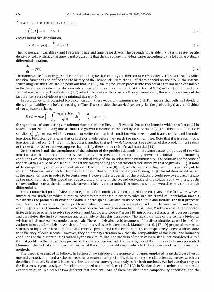
where for the upwind method hj = h and L = J + J∗, and for the characteristics scheme L = JĎ + 1. In Fig. 2, we presentthe results obtained by means of the characteristics scheme, T = 1000 and k = 0.03125. The upwind method gives thesame plot. Furthermore, we approximate the Malthusian parameter by means of a least squares technique using the Matlabroutine lsqcurvefit. Thus, in the case of the first test problem, we obtain for both schemes approximations to bothparameters C and σ . If we use T = 1000, h = 0.003125, k = 0.01389, for the upwind method we have C = 0.0272,σ = 0.0621; and using T = 1000 and k = 0.03125 for the characteristics scheme we obtain C = 0.0271, σ = 0.0616. Ifwe employ a different initial condition (u(x, 0) = 2ϕ(x)), C = 0.0541 with the upwind method and C = 0.0540 with thecharacteristics scheme and the estimation computed for σ is the same.A validation of the approximations obtained for the Malthusian parameter and the stable size distribution is given by

testing their relationship with the corresponding eigenvalue problem. The value (1 + σ k) is a good approximation to the

662 L.M. Abia et al. / Mathematical and Computer Modelling 50 (2009) 653–664

01

0.80.6

0.40.2

0 1000800

600

timecell size

freq

uenc

y

400 2000

1

2

3

4

5

6

Fig. 2. Frequency distribution of the evolution of the cell population computed with the characteristics method, T = 1000 and k = 0.03125.

0.46 0.48 0.5 0.52 0.54

At x=1/2. Upwind Method.

0.78 0.8 0.82 0.84

0

5

10

15

20

Along Characteristic that begins at x=1/2. Upwind Method.

0.46 0.48 0.5 0.52 0.54

At x=1/2. Characteristics Method.

0.78 0.8 0.82 0.84

Along Characteristic that begins at x=1/2. Characteristic Method

–12

–10

–8

–6

–4

–2

0

–12

–10

–8

–6

–4

–2

0

0

10

20

30

40

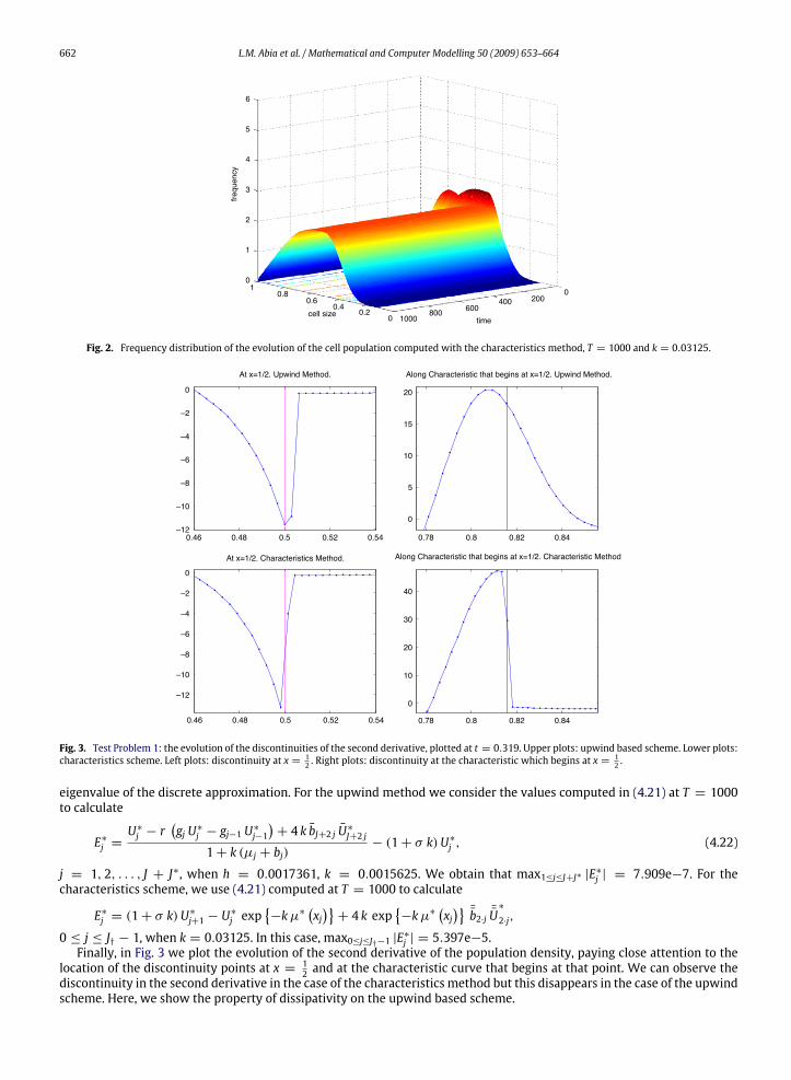
Fig. 3. Test Problem 1: the evolution of the discontinuities of the second derivative, plotted at t = 0.319. Upper plots: upwind based scheme. Lower plots:characteristics scheme. Left plots: discontinuity at x = 1

2 . Right plots: discontinuity at the characteristic which begins at x =12 .

eigenvalue of the discrete approximation. For the upwind method we consider the values computed in (4.21) at T = 1000to calculate

E∗j =U∗j − r

(gj U∗j − gj−1 U

∗

j−1

)+ 4 k bJ+2 j U∗J+2 j

1+ k (µj + bj)− (1+ σ k)U∗j , (4.22)

j = 1, 2, . . . , J + J∗, when h = 0.0017361, k = 0.0015625. We obtain that max1≤j≤J+J∗ |E∗j | = 7.909e−7. For thecharacteristics scheme, we use (4.21) computed at T = 1000 to calculate

E∗j = (1+ σ k)U∗

j+1 − U∗

j exp{−kµ∗

(xj)}+ 4 k exp

{−kµ∗

(xj)}¯b2·j ¯U

∗

2·j,

0 ≤ j ≤ JĎ − 1, when k = 0.03125. In this case, max0≤j≤JĎ−1 |E∗

j | = 5.397e−5.Finally, in Fig. 3 we plot the evolution of the second derivative of the population density, paying close attention to the

location of the discontinuity points at x = 12 and at the characteristic curve that begins at that point. We can observe the

discontinuity in the second derivative in the case of the characteristics method but this disappears in the case of the upwindscheme. Here, we show the property of dissipativity on the upwind based scheme.

L.M. Abia et al. / Mathematical and Computer Modelling 50 (2009) 653–664 663

First Derivative. Along Characteristic that begins at x=a/2.

0.34 0.36 0.38 0.4 –5

0

5

10

15

20

25

Second Derivative. Along Characteristic that begins at x=a/2

0.46 0.48 0.5 0.52 0.54

Second Derivative. At x=1/2.

0.6 0.62 0.64 0.66

Second Derivative. Along Characteristic that begins at x=1/2

0.34 0.36 0.38 0.4

–2

0

2

4

6

8

10

12

0.5

1

1.5

2

2.5

3

–24

–22

–20

–18

–16

–14

–12

–10

Fig. 4. Test Problem 2: evolution of the discontinuities for the upwind method, plotted at t = 0.365. Upper plots: discontinuity of the first (on the left)and second (on the right) derivatives along the characteristic curve that begins at x = a

2 . Lower plots: discontinuities of the second derivatives at x =12

(on the left) and along the characteristic curve that begins at x = 12 (on the right).

0.54 0.56 0.58 0.6

First Derivative. Along Characteristic that begins at x=a/2.

0.54 0.56 0.58 0.6

Second Derivative. Along Characteristic that begins at x=a/2

0.46 0.48 0.5 0.52 0.54

–14

–12

–10

–8

–6

–4

–2

0

Second Derivative. At x=1/2.

0.72 0.74 0.76 0.78

Second Derivative. Along Characteristic that begins at x=1/2

–0.5

0

0.5

1

1.5

2

2.5

3

3.5

0

100

200

300

400

500

600

–5

0

5

10

15

20

25

30

35

Fig. 5. Test Problem 2: evolution of the discontinuities for the characteristics scheme, plotted at t = 0.565. Upper plots: discontinuity of the first (on theleft) and second (on the right) derivatives along the characteristic curve that begins at x = a

2 . Lower plots: discontinuities of the second derivatives atx = 1

2 (on the left) and along the characteristic curve that begins at x =12 (on the right).

In Figs. 4 and 5, we present the first and second derivatives of the density distribution of the solution at t = 0.365 andt = 0.565 for the upwind method and the characteristics scheme, respectively. In these figures, we plot the discontinuitiesof the derivatives. We observe how the behaviour is better for the solution given by the characteristics scheme than for theupwind basedmethod because the characteristics scheme conserves them. Again, this shows the dissipativity of the upwindbased scheme.

664 L.M. Abia et al. / Mathematical and Computer Modelling 50 (2009) 653–664

Acknowledgements

The authors were supported in part by the project of the Ministerio de Educación y Ciencia MTM2008-06462-C02-02,FEDER, by the project of the Junta de Castilla y León and Unión Europea F.S.E. VA046A07 and by the 2009 Grant Program forExcellence Research Group (GR137) of the Junta de Castilla y León.

References

[1] G.I. Bell, E.C. Anderson, Cell growth and division, I. A mathematical model with applications to cell volume distributions in mammalian suspensioncultures, Biophys. J. 7 (1967) 329–351.

[2] G.I. Bell, Cell growth and division, III. Conditions for balanced exponential growth in a mathematical model, Byophys. J. 8 (1968) 431–444.[3] A.G. Fredrickson, D. Ramkrishna, H.M. Tsuchiya, Statistics and dynamics of procaryotic cell populations, Math. Biosci. 1 (1967) 327–374.[4] J.W. Sinko, W. Streifer, A model for populations reproducing by fission, Ecology 52 (1971) 330–335.[5] O. Diekmann, H.J.A.M. Heijmans, H.R. Thieme, On the stability of the cell size distribution, J. Math. Biol. 19 (1984) 227–248.[6] J.A.J. Metz, O. Diekmann (Eds.), Dynamics of Physiologically Structured Populations, in: Lecture Notes Biomath, vol. 86, Springer-Verlag, New York,1986.

[7] A. Lasota, M.C. Mackey, Probabilistic Properties of Deterministic Systems, Cambridge University Press, London, 1985.[8] A. Lasota, M.C. Mackey, Chaos, Fractal and Noise. Stochastic Aspects of Dynamics, in: Appl. Math. Sci., vol. 97, Springer-Verlag, New York, 1994.[9] B. Perthame, Transport Equations in Biology, Birkhäuser, Basel, Switzerland, 2007.[10] K.E. Howard, A size-structured model of cell dwarfism, Discrete Contin. Dyna. Syst. B 4 (3) (2001) 471–484.[11] B. Perthame, J.P. Zubelli, On the inverse problem for a size-structured population model, Inverse Problems 23 (2007) 1037–1052.[12] A.J. Fabens, Properties and fitting of the von bertalanffy growth curve, Growth 29 (1965) 265–289.[13] J.M. Cushing, An Introduction to Structured Population Dynamics, in: CMB-NSF Regional Conference Series in Applied Mathematics, SIAM, 1998.[14] J.J. Liou, F. Srienc, A.G. Fredrickson, Solutions of population balance models based on a successive generations approach, Chem. Eng. Sci. 52 (1997)

1522–1540.[15] N.V. Mantzaris, J.J. Liou, P. Daoutidis, F. Srienc, Numerical solutions of a mass structured cell population balance model in an environment of changing

substrate concentration, J. Biotech. 71 (1999) 157–174.[16] O. Angulo, J.C. López-Marcos, A numerical scheme for a size-structured cell population model, in: V. Cappasso (Ed.), Mathematical Modelling and

Computing in Biology and Medicine, Esculapio, Bolonia, 2003, pp. 485–496.[17] N.V. Mantzaris, P. Daoutidis, F. Srienc, Numerical solutions of multi-variable cell population balance models, I. Finite difference methods, Comput.

Chem. Eng. 25 (2001) 1411–1440.[18] N.V. Mantzaris, P. Daoutidis, F. Srienc, Numerical solutions of multi-variable cell population balancemodels, II. Spectral methods, Comput. Chem. Eng.

25 (2001) 1441–1462.[19] N.V. Mantzaris, P. Daoutidis, F. Srienc, Numerical solutions of multi-variable cell population balance models, III. Finite element methods, Comput.

Chem. Eng. 25 (2001) 1463–1481.[20] K. Ito, F. Kappel, G. Peichl, A fully discretized approximation scheme for size-structured population models, SIAM J. Numer. Anal. 28 (1991) 923–954.[21] O. Angulo, J.C. López-Marcos, Numerical schemes for size structured population equations, Math. Biosci. 157 (1999) 169–188.[22] N. Keyfitz, Introduction to the Mathematics of Population, Addison Wesley, 1968.[23] F. Hoppensteadt, Mathematical Theories of Populations: Demographics, Genetics and Epidemics, SIAM, 1975.[24] O. Angulo, J.C. López-Marcos, F.A. Milner, The application of an age-structured model with unbounded mortality to demography, Math. Biosci. 208

(2007) 495–520.