numerical simulation of the flow field in a friction-type ... · bladeless turbine; instead of...
TRANSCRIPT

DIPLOMA THESIS
Numerical Simulation of the Flow Field in a Friction-Type Turbine (Tesla Turbine)
written at the Institute of Thermal Powerplants
Vienna University of Technology
by Andrés Felipe Rey Ladino
National University of Colombia, School of Engineering Calle 57c No. 40-51 Ap. 419, Bogotá, Colombia,
supervised by Ao.Univ.Prof. Dipl.-Ing.Dr. Reinhard Willinger
Vienna University of Technology Institute of Thermal Powerplants
and
Prof. Engineer Javier Castro Mora
National University of Colombia, School of Engineering.
Vienna, 14th June 2004

Abstract In this Diploma thesis the results of the investigation of a Numerical Simulation of the Flow Field in a Friction-Type Turbine is presented. The Tesla turbine, an unconventional turbomachinery that uses smooth disks instead of blades, is described principally by the loading coefficient curve, the efficiency and degree of reaction vs. the flow rate parameter. In order to describe its behaviour, the rotational speed is maintained constant and the flow rate is changed with the purpose of simulate a virtual brake, and obtain the performance curves of the Tesla turbine. Since the flow is characterized in a transitional regime, both laminar and turbulent cases are simulated. The work presented represents an initial significant step towards the analysis of this type of flow using CFD tool. Starting from a simple axi-symmetric model of the flow between two co-rotating disks in two dimensions, the model is improved including the outlet of the turbine with the casing, and at the end a 3D simulation of a single disk is performed including the effects of the nozzles. A complete model of a Tesla turbine is restricted by computer resources.
Kurzfassung In dieser Diplomarbeit werden die Ergebnisse der Untersuchung einer numerischen Simulation der Strömung in Reibungsturbomaschinen dargestellt. Die Tesla Turbine, eine unkonventionelle Turbomaschine, welche glatte Scheiben anstelle der Blätter benutzt, wird hauptsächlich durch die wichtigsten Parameter, d.h. Leistungskoeffizient, Wirkunsgrad und Reaktionsgrad gegen die Durchflusszahl gekennzeichnet. Um das Verhalten dieser Turbomaschine zu beschreiben, wird die Winkelgeschwindigkeit konstant gehalten, und die Durchflusszahl geändert, um die Kennlinien der Tesla Turbine zu erreichen. Damit wird eine virtuelle Bremse simuliert. Da die Strömung vom Übergangsmodel bestimmt ist, werden sowohl der laminare, als auch der turbulente Fall simuliert. Die vorliegende Arbeit stellt einen ersten bedeutenden Schritt in Richtung einer Analyse dieser Art der Strömung mit CFD als Werkzeug dar. Ausgehend von einem einfachen achssymmetrischen Modell der Strömung zwischen zwei rotierenden Scheiben in zwei Dimensionen, wird das Modell mit dem Ausgang der Turbine und einem teil des Gehäuses erweitert. Als letztes Modell wird eine 3D Simulation von einer einzigen Scheibe durchgeführt, welches die Effekte der Düsen berücksichtigt. Die genaue Simulation eines kompletten Modells einer Tesla Turbine ist durch die vorhandenen Computerressourcen eingeschränkt.
Resumen En esta tesis de investigación se presentan los resultados obtenidos de la simulación numérica del campo de velocidades y del flujo en una turbina de fricción. La turbina Tesla, una turbomáquina poco convencional que utiliza diskos planos y lisos en lugar de álabes, es caracterizada principalmente por la curva de coeficiente de carga, la eficiencia y el grado de reacción contra el coeficiente volumétrico. Para describir su comportamiento, la velocidad angular se mantiene constante y el caudal se varia con el propósito de simular un freno virtual, obteniéndose las curvas de funcionamiento de la turbina Tesla. Puesto que el flujo se encuentra en régimen transitorio, se simulan ambos casos laminar y turbulento. Este trabajo representa un paso inicial significativo hacia el análisis de este tipo de flujo usando CFD como herramienta. Comenzando desde un modelo simple axisimétrico del flujo entre dos diskos corotantes en dos dimensiones, el modelo se mejora incluyendo la salida de la turbina y parte de la carcaza, y finalmente se realiza una simulación 3D de un solo disko que incluye los efectos de las toberas. Un modelo completo de la turbina Tesla es restringido por recursos computacionales.
i

Acknowledgments The present Diploma thesis was carried out in winter and summer semester 2003-2004 at the Institute of Thermal Powerplants at the University of Technology of Vienna (Austria). I sincerely thank Em. o.Univ.Prof. Dipl.Ing. Dr.techn. Hermann Haselbacher for the opportunity to work at this Institute and for his sponsorship. I would like to express my gratitude to Ao.Univ.Prof. Dipl.Ing. Dr.techn. Reinhard Willinger for all the support, trust, supervision and opportune guidance in this thesis. Without his explanations, opinions, and contributions, this work could never have been possible. I also thank to Prof. Engineer Javier Castro Mora, for his support and advice from Colombia, Ing. Gerhard Kanzler, Univ.Ass. Dipl.Ing. Klaus Hörzer, Univ.Ass. Dipl.Ing. Dr.techn. Franz Wingelhofer, and Hr. Franz Trummer for their constant support and cordiality. To the seminar students and diplomanden and to Gustavo Cañón. I enormously appreciated the help and hospitality that family Krenn showed me at every time, finally I sincerely thank all the students and people I met in Vienna, specially Aurore Desavoye and Barbara Windtner for the corrections made, and for the time we spend together and help in the good and bad moments, these times will always remained in my mind. I dedicated this work to my parents and my brothers. They are my deepest motivation, for continuing working. Thank you for all your encouragements and motivation. To all the foregoing and also they who are not mentioned here I extend my sincere thanks. Dedico este trabajo a mi familia , y les doy mi más sincera gratitud por todo su apoyo, ánimo, fortaleza y por todas sus oraciones y esfuerzos. A Helen por su Amor. Finalmente doy Gracias a Dios Padre, a Jesús y al Espíritu Santo quienes hacen posible todas las cosas.
ii

Preface The simulation could be defined as the admirable method of learning
by doing. Jakub Polkowski.
Nikola Tesla, one of the geniuses of our century contributes in many fields of the technique. He was born in Smiljan, former part of Austrian-Hungary empire (actually Croatia) in 1856, and he died in New York, EEUU in 1943. Between his prolific inventions it is found the bladeless turbine; instead of using fan-type blades, Tesla turbine utilized solid disks of metal, and relied on what is called the boundary layer effect. His turbine ran on either compressed air or steam. This machine is the subject of this work, in which CFD –Computational Fluid Dynamics- tool is used in order to solve the mathematical equations that govern the fluid. Researches on this topic have been made from different initial statements and the results are diverse. Many analytical and experimental efforts and achievements have been made on this field but at the present no much works using CFD have been published. This work does not pretend to answer all the questions that have been formulated for the Tesla turbine, but an approximation of the “analytically unsolved Navier-Stokes equations” using Fluent Software. The Tesla turbomachinery is a new topic in the Institute of Thermal Turbomachines and Powerplants, and it has been support by the National University of Colombia and the Vienna University of Technology. It has been extensively studied in EEUU, Germany and Japan as well as others studies have appeared in other nations as France, Canada, India and the United Kingdom. The applications of the principle that this turbine uses are wide and the future will undertake the development of this unconventional turbine. The search of new sustainable ways of managing the energy on the world will take us to the analysis of new machines that are able to deal with new form of production and energy transformation.
iii

Contents
1. Introduction ........................................................................................................................ 1
2. Literature Review............................................................................................................... 2
2.1. Introduction and History of the Tesla Turbine........................................................... 2
2.2. Analytical and Experimental Literature Review........................................................ 3
2.3. Stability of Laminar Flow .......................................................................................... 8
2.4. One Dimension Model ............................................................................................... 9 3. Description of the Tesla Disk Turbine ............................................................................. 11
3.1. Geometrical, Dynamic and Physical Operation Description ................................... 11
3.2. Dynamic and Operation Description........................................................................ 13
3.3. Characterization of the Flow.................................................................................... 15
3.4. Reversibility of Operation........................................................................................ 16
3.5. Losses ....................................................................................................................... 16
3.6. Advantages ............................................................................................................... 18
3.7. Disadvantages........................................................................................................... 20
3.8. Actual Tesla-Type Machines ................................................................................... 20 4. Fluid Dynamics ................................................................................................................ 22
4.1. Control Volume Concept ......................................................................................... 22
4.2. Non-dimensional Analysis ....................................................................................... 24
4.2.1. Geometrical Similarity ............................................................................. 27
4.2.2. Flow Regime Similarity ........................................................................... 27
4.2.3. Non-dimensional Performance Parameters .............................................. 29 4.3. Laminar Flow ........................................................................................................... 32
4.4. Swirling and Rotating Flows.................................................................................... 33
4.5. Navier Stokes Equations .......................................................................................... 33
4.5.1. Momentum Conservation Equation for swirl Velocity ............................ 34
4.6. Turbulence, The Reynolds–Averaged Equations..................................................... 34
4.7. Transition ................................................................................................................. 36
4.7.1. Modes of Transition ................................................................................. 38
4.8. Relaminarization ...................................................................................................... 38
4.9. Theory of Boundary Layer....................................................................................... 38 5. Modeling in CFD and Results.......................................................................................... 41
5.1. The Models and their Limitations ............................................................................ 41
5.2. Built of the Model .................................................................................................... 42
iv

5.3. Geometry.................................................................................................................. 42
5.4. Restrictions of the Grid ............................................................................................ 43
5.5. Mesh ......................................................................................................................... 43
5.6. Convergence............................................................................................................. 47
5.7. Working Fluid Properties ......................................................................................... 47
5.8. Boundary Conditions................................................................................................ 48
5.9. Laminar Solution...................................................................................................... 48
5.9.1. Convergence of Laminar Solution ........................................................... 48
5.9.2. Post-processing of the Laminar Solution ................................................. 50
5.10. Comparison Results with Experiment for Selection of the Turbulence Model ... 58
5.11. Turbulent Solution................................................................................................ 61
5.11.1. Numerical Characterization of the Relaminarization............................... 71
5.12. Simulation of the Turbine with Full Peripheral Admission. ................................ 72
5.13. 3D Slide Model, Simulation and Results ............................................................. 82
5.13.1. Setting up of 3D slide model.................................................................... 86
5.13.2. Boundary conditions ................................................................................ 86
5.13.3. Convergence............................................................................................. 87
5.13.4. Results ...................................................................................................... 88 6. Discussion and Conclusions............................................................................................. 94
6.1. Discussion ................................................................................................................ 94
6.2. Future Work ............................................................................................................. 96
Appendix A .............................................................................................................................. 97 Tesla Turbomachinery Tested and Reported in Technical Papers ........................... 97
Appendix B ............................................................................................................................ 100 Variation of Reynolds Number in the Flow Between two Disks........................... 100
Appendix C ............................................................................................................................ 101 1. Low Reynolds Number Effects and Turbulence Low Re k-� Model................. 101 2. Launder-Sharma Model...................................................................................... 101
Bibliography........................................................................................................................... 102 Literature about Turbines ....................................................................................... 102 Literature about Tesla Pumps................................................................................. 104
List of Figures ........................................................................................................................ 106
List of Tables.......................................................................................................................... 108
v

Notation and Nomenclature Latin characters Symbol Unit Description
A [ ] Area. 2mB [ ] Body force per unit area / mass. Nb [ ] Spacing between disks. m
���� ,21 ,,, kCCC [-] Constant in Reynolds stress k-� equations.
c [ sm ] Total Velocity (Velocity Magnitude ).
e [ kgKJ ] Specific internal energy.
F [ ] Force due to flow, External force per unit area / mass. Nf,g [-] Functions. h [ kg
KJ ] Specific enthalpy.
K [-] Acceleration parameter
k [ 22
sm ] Specific turbulent kinetic energy.
L [-], [m] Characteristic length, length. Ma [-] Mach number. M [kg] Mass. m� [ s
kg ] Mass flow rate.
N [-] Property of a system. n [-] Specific property of a system. Normal vector.
P [W , HP], [ 32
sm ] Power, turbulent production rate.
p [Pa],[-] Pressure, Pohlhausen parameter. q [ kg
KJ ] Energy rate transfer.
Q [ sm3 ] Volume flow rate between disks.
r [ ] General radial coordinate. mR [ Kkgmol
KJ�
],[-] Universal constant of gases, degree of reaction.
Re [-] Reynolds number. s [ kg
KJ ] Specific entropy.
t [ s ],[m] Time, width of plate. T [°C, K] Temperature. T [N-m] Torque. TI [%,-] Turbulence intensity. U� [-] Velocity wall friction u,U [ s
m ] Radial component of velocity.
vi

v,V [ sm ], [ ] Tangential (Swirl) component of velocity, Volume. 3
m
w,W [ sm ] Axial component of velocity.
x [-] Cartesian coordinate, variable, �-exponent. y [-] Cartesian coordinate, �-exponent. z [-] Cartesian coordinate, �-exponent.
Greek Characters Symbol Unit Description
�� � [-] Viscogeometric parameter.��� [°] Angle between the tangential and magnitude component
of velocity; at station 1 is the angle of the nozzle. �� [-] Variable for Kronecker delta function, thickness of
boundary layer. �* [-] Moment thickness of the boundary layer �� [ 3
2
sm ] Specific turbulent dissipation rate.
� [-] Ratio of specifics heats. �� [%] Efficiency. [-] Flow coefficient. � � �� � � � Loading coefficient.��� [ sPa � s
m�kg ] Viscosity of fluid. �� [ s
m2 ] Kinematic viscosity of fluid. �� [-] ���Buckhingam numbers. �� [ 3m
kg ] Density of fluid. �� [Pa] Reynolds stress. � [Pa] Shear stress. ����� [ s
rad ] Angular velocity.
Subscripts Symbol Description
0 Inlet station at the nozzle 1,o Inlet station of the rotor (outer) 2,i Outlet station of the rotor (inner) A Available b Related to the gap D Related to flow in pipe d Related to the disk e Effective
vii

�� Freestream flow i,j Coordinates in tensorial form k Kinetic N Net r Radial direction, Related to the radius rel Relative s Isentropic, static t Stagnation condition, total t Turbulent tr Transition w Wall � Dissipative �� t� Tangential direction � Related to the angular speed
Upscripts Symbol Description
� Average value in time �� Variable for the nozzle, fluctuations of turbulent velocity ��� Variable for the rotor �� Variable per unit of time
*� Non-dimensional variable + Sublayer-scaled value t Turbulent
Abbreviations 2D Two dimensions 3D Three dimensions CFD Computational Fluid Dynamics CS Control Surface CV Control Volume GUI Graphical User Interface k-� (turbulent) Kinetic energy / dissipation model NS Navier Stokes RANS Reynolds Average Navier Stokes TI Turbulence Intensity
viii

Chapter 1 1. Introduction The flow inside a Tesla Turbine as well as the flow of a fluid between two parallel corotating disks is of general interest in the technical field. The turbomachinery applications have several variants, each idea comes to help to construct the world of power. One of this ideas was put into real world by Nikola Tesla, in his application of a friction turbine, with new concepts of energy transfer, using the properties of the fluids as viscosity, adhesion and cohesion instead of the conventional energy transfer mechanism in bladed turbines. The application of this special turbine is not on the normal spectrum range of turbomachinery for as powerplants or aeroderivative turbines, but its use is intended for small applications. Different concepts and theories have been used to explain the behaviour of this machine in the analytical field, besides the physical testing has been also used by researches, and with the upcoming of the computer age and the availability of numerical methods, the numerical solution has been conducted over an extensive formulation of the NS equations using several methods and assumptions. In the present work CFD tools are used to understand the overall flow inside the turbine. It presents the numerical simulation of the flow field in a friction-type turbine. The commercial Computational Fluid Dynamics code FLUENT as well as the grid generation software GAMBIT have been used for the investigation. The aim of the work is to provide an objective point of view of the flow in 2D and 3D flow space. With a selected turbine configuration, which is supported by experimental flow results, is showed a 2D simulation over an isolated rotor (flow between two disks). It is important to state that the analysed geometry is not optimised, as the researcher of this turbine states in reference [32], who takes the initial geometry from the patent of Tesla [37]. In addition, the CFD method is used to compute the flow field in a Tesla turbine consisting of rotor and stator (nozzles), using the 3D capabilities of modern computational fluid dynamics codes for complicated 3D-geometries. The computed results are analysed and compared with theoretical and experimental facts gained from the literature. The modelling of the 3D flow in the whole turbine is of great practical relevance but the limitation and restrictions of computer resources dictate a different approach of modelling this turbine instead of simulating a complete 3D model. The obtained results are diskussed. The work concludes with a summary of conclusions and some guidelines concerning future flow research on this field.
1

Chapter 2 2. Literature Review This chapter presents a short history of this turbomachine and a summary of some of the works conducted by different researches of Tesla turbine; they described the analytical approach as well as experimental results. 2.1. Introduction and History of the Tesla Turbine One of the inventions that the engineer and inventor Nikola Tesla conceived was the Tesla disk turbine. With this device he proposed to make an useful and efficient handle of the energy especially on electric generation, fluid power and engines field. Therefore, the Tesla turbine also called and denoted in literature as Tesla turbomachines, multiple-disk, shear, shear force or boundary layer turbomachinery, is a rotatory fluids machine that works with compressible and incompressible fluid. The direction of the fluid flows in the radial and tangential direction, forming spirals streamwise and operates principally on the laminar regime. He referred to it as a thermodynamic converter in his original patented. More over of conceiving the Tesla turbine, Nikola Tesla provided an useful design for other machines operating the principle of the Tesla disk. Examples of these machines are an air compressor, an air motor engine, a vacuum exhauster or vacuum pump. These machines use the Tesla method of “fluid propulsion” that is based on two basic principals of physics of the fluids: “adhesion and viscosity”. These types of turbomachinery can be applied as liquid pumps, liquid or vapor or gas turbines, and gas compressors [37]. On October 21st, 1909 Nikola Tesla filled a patent for a pump, which uses smooth rotating disks inside a volute casing. In the patent (which he received May 6th, 1913, U.S. Patent No.1,061,142) Tesla began by pointing out the benefits of a smooth transition of energy: "In the practical application of mechanical power based on the use of fluid as the vehicle of energy, it has been demonstrated that, in order to attain the highest economy, the changes in velocity and direction of movement of the fluid should be as gradual as possible." The Tesla turbine invention was discussed in the semitechnical press at the time of the invention [13-40]. What Tesla claims in his patents was a high efficiency due to the form of energy transfer, based on the assumption that a highest economy will be attained when the changes in velocity and direction of the movement of the fluid is as gradual as possible. This can be accomplished causing the propelling fluid moving in natural paths or streamlines of least resistance, free from constraints and disturbances caused by vanes or intricate devices in common turbomachinery, and changing the fluid velocity and direction of movement by imperceptible degrees.
2

2. LITERATURE REVIEW
Figure 2.1. American patent No. 1,061,206 of Tesla turbine [37].
Besides, the employment of the usual devices for deriving energy from a fluid, such a pistons, paddles, naves and blades, necessarily introduces numerous limitations, constraints and adds to the complication, cost of production and maintenance of the machines. The idea of Tesla, was to incorporate this turbine to the Wandercliff project where he expected to deliver a low cost energy for popular use. Then, his first prototypes were big in size, and the success for high power was not achieved; the Allis Chalmers Company also bet for this design and built a friction turbine, and later ceased their tests because of the low efficiency obtained for big sizes and early problem with the materials [29]. 2.2. Analytical and Experimental Literature Review Tesla conducted experiments of his turbine between 1906 and 1914 [38], then there was little activity on this field until a revival of interest began in the 50´s. After that, research was widespread in analytical field [28-6,5,22,18,14,23], experimental tests [13,1,32,2,27] and recently CFD modelling of the flow in the space between two disks in a rotor [30,14,68,72]. The research began with studies on disk rotating inside a fluid for brake systems [13] and for coupling systems, an analytical concept approaches as well as approximations of the behaviour of the disk resistance due to the friction and overall parameters such torque and power [28]. Later, different methods were used for the solution of the flow field with an approach with friction factors in order to simplify the Navier-Stokes (NS) equations [32]; with the availability of numerical methods, the numerical solution was conducted over an extensive formulation of the NS equations using several schemes, methods and assumptions, first with laminar flow and on the 80´s years with turbulent considerations [11,47,48,72]. Analytical researches on the following topics for the Tesla turbine are available:
3
2. LITERATURE REVIEW
�� Laminar approach [24,6,5,22,18,42,15,43]. �� Turbulent approach [11,47,48,72]. �� Solution with incompressible fluid [most of literature]. �� Solution with compressible fluid [18,43,30]. �� Heat transfer in frictions turbines [15,14] �� Multiphase fluids [43,42]
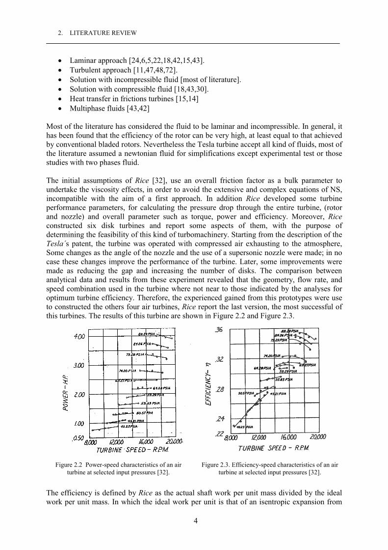
Most of the literature has considered the fluid to be laminar and incompressible. In general, it has been found that the efficiency of the rotor can be very high, at least equal to that achieved by conventional bladed rotors. Nevertheless the Tesla turbine accept all kind of fluids, most of the literature assumed a newtonian fluid for simplifications except experimental test or those studies with two phases fluid. The initial assumptions of Rice [32], use an overall friction factor as a bulk parameter to undertake the viscosity effects, in order to avoid the extensive and complex equations of NS, incompatible with the aim of a first approach. In addition Rice developed some turbine performance parameters, for calculating the pressure drop through the entire turbine, (rotor and nozzle) and overall parameter such as torque, power and efficiency. Moreover, Rice constructed six disk turbines and report some aspects of them, with the purpose of determining the feasibility of this kind of turbomachinery. Starting from the description of the Tesla´s patent, the turbine was operated with compressed air exhausting to the atmosphere, Some changes as the angle of the nozzle and the use of a supersonic nozzle were made; in no case these changes improve the performance of the turbine. Later, some improvements were made as reducing the gap and increasing the number of disks. The comparison between analytical data and results from these experiment revealed that the geometry, flow rate, and speed combination used in the turbine where not near to those indicated by the analyses for optimum turbine efficiency. Therefore, the experienced gained from this prototypes were use to constructed the others four air turbines, Rice report the last version, the most successful of this turbines. The results of this turbine are shown in Figure 2.2 and Figure 2.3.
Figure 2.2 Power-speed characteristics of an air
turbine at selected input pressures [32]. Figure 2.3. Efficiency-speed characteristics of an air
turbine at selected input pressures [32].
The efficiency is defined by Rice as the actual shaft work per unit mass divided by the ideal work per unit mass. In which the ideal work per unit is that of an isentropic expansion from
4

2. LITERATURE REVIEW
the actual turbine inlet temperature and pressure to the actual turbine exhaust pressure, with zero velocity assigned the flow at the beginning and end of the isentropic expansion. Rice developed a simple initial analysis using pipe flow theory with bulk coefficients for friction that gives some qualitative understanding through graphs as it is shown in Figure 2.4 and Figure 2.5. With this graphs it is possible to obtain approximate values of efficiencies for different flow rates, but for the specified geometry ro/b= 50.
Figure 2.4.: Typical results for maximun efficiency as a funtion of flow rate and speed parameter. Plotted for
f=0.05, ro/b=50 [32].
Figure 2.5.: Typical results for pressure-change parameter as a function of flow rate and speed parameters. Plotted for f= 0.05, ro/b=50 [32].
Figure 2.4 shows that high efficiencies is only obtain for very low flow rates at values of
0001.03�� orQ , and the second turbine tested by Rice has a value of 01256.03
�� orQ , then, the efficiencies are expected to be under 40% as it is shown in Figure 2.4. Figure 2.5 depicts the change of pressure, for higher tangential velocities, the change of pressure is higher, and for higher flow rates the change of pressure is lower, this is because the change of pressure occurs only in the boundary layer due to the effects of viscosity and with the increase of flow rate, the velocity increase and the thickness or region of the boundary layer diminishes. Other multiple disk friction turbine was tested and reported by Elkouh et al. [1]; they remark that with this configuration, the disks would not have bending loads and can support higher temperatures using the high temperature characteristics of ceramics and avoids the low ductility problem set by these materials. They reports a maximum turbine efficiency of 41 percent. Other analytical approaches were made with numerical methods; a finite difference scheme for calculating the radial outward flow between corotating disks was presented by Breiter and Pohlhausen [50], a similar method of calculation was applied for radially inward flow by Boyd and Rice [6] using finite difference solution, which modelled the inlet region of the
5

2. LITERATURE REVIEW
turbine, and take into account the inner region which develop an asymptotic flow, solution for flow with high Reynolds number. They report at inner radii, away from the inlet, some asymptotic field with high local Reynolds number and furthermore, they hypothesized that in a region where an inflection of the radial velocity profile is presented, the flow will undergo transition from laminar flow to turbulent flow. In addition, they also stated that with the same flow parameter Uo
* and Vo*, and Reynolds number Reb, associated to the gap (for an
explication of non-dimensional numbers see section 4.2.2), the fields computed at inner radii were independent of the distributions of the settled profiles at the inlet of the rotor: u(z) for radial and v(z) for tangential. It is interesting that for the flow between disks exist several different phenomena for the field flow. These conditions are turbulent inlet, laminarization from turbulent to laminar due to thickness of boundary layer, inflection of the profile, forward transition, acceleration of the flow due to continuity and conservation of angular momentum, creating a free vortex flow near the inner radius of the disk with high local Reynolds number and reverse transition or relaminarization. Matsch and Rice [24] performed a analytical treatment using and asymptotic solution for laminar and incompressible, their results show some kind of inflection at r = 0.15 and show the acceleration of the flow starting at a radius of 0.4 which agree with the results of Boyd naming it as the asymptotic flow region, and because of this special behaviour, Murata [62] proposed to divide the domain in three regions to overcome the difficulty of the slow convergence at inlet and outlet stations in the following way: for the entrance Görtler series was applied, at the inner region, the analytical perturbation solution was utilized, and for the mid region that connects the two extremes an implicit finite difference was used. For the purpose of comparing all analytical data generated by several methods and researches, and to overcome with the questions of transition and inflection, Adams and Rice [2] performed a experiment over an isolated disk, inward flow in which the fluid entry at the periphery with a certain pressure and velocity and the disks are driven by a motor; this means that is not the configuration of a turbine but rather the sink flow configuration. In this research the parameter for characterizing the flow are the Reb, the flow parameter Uo
* and the tangential velocity Vo
*. He reports the static pressure difference along the radius. Adams and Rice did not report velocities profile in his investigation due to the lack of accurately instruments for smalls gaps without introducing errors in the measurement. Between his conclusions stated that very near the outer periphery, the analytical curve do not lie on the experimental results primarily because of partial admission effects due to the finite nozzle configuration and besides the presence of effects of laminarization and relaminarization. Adams and Rice proposed a limit for the laminar flow assuming that the inflection of the profile is the initial of instabilities, and this occurs approximately at a Reb=10, since all calculated radial velocity profiles are after that inflected. The characteristics of the tested turbines are summarized in the Table 2.1. An explication of the different numbers reported here is given in the section 4.2.2 non-dimensional analysis.
6

2. LITERATURE REVIEW
Reference Research topic Fluid r1/b r1/r2 Re� Rer Reb Mach
1 Warren Rice, 1965.
Flow between Corotating disk, Turbine air 56 5.30 8,850 496,000 158 0.26
2 Warren Rice, 1965.
Flow between Corotating disk, Turbine air 87 5.30 5,215 456,000 60 0.24
3 Warren Rice, 1965.
Flow between Corotating disk, Turbine air 200 6.06 5,180 1,036,000 25.91 0.48
4 A.F. Elkouh : 1961 Gas Turbine for High temperatures air 79.5 1.64 9,000 719,300 113.8 0.24
5 R.Adams, W. Rice 1970
Driven Flow between Corotating disk Sink Flow (Turbine effect)
water-ethylene glycol 133 8.00 97,200 12,971,700 729.6 0.21
6 Nendl, D. 1973 Friction Turbine water Comparison - 2.5- - 4.3 -
7 Nendl, D. 1973 Friction Turbine Oil Comparison - 2.5- - 12.8 -
Table 2.1. Non-dimensional parameters and characteristics of tested turbines.
One of the conclusions of Rice is that the results indicate that multiple disks turbines may be attractive and feasible in the low power part of turbines applications, with small configurations. The gap distance as well as his relation with the Reynolds number Reb cannot be found by methods of high efficiency because at maximum efficiency there is no trade of energy, and this relations have been studied by Lawn and Rice [22], in order to give some maps and data of the turbine with a incompressible fluid for an optimum design. These maps show the quantitative dependence of turbine efficiency, total pressure and delivered power on the turbine geometry and speed on the tangential and radial velocity, in other words on the nozzle direction, and also on the Reynolds number or fluid properties. Lawn and Rice concluded from his work that the greatest efficiency occurs near a value of Reb=4 for low radial velocity obtained with small angles of the nozzle. Figure 2.6 shows one of the solution of Lawn and Rice, in which can be seen that high efficiencies are obtain with low flow coefficient.
Figure 2.6.: Constant efficiency lines on Re and Uo*, for Vo*= 1.1, r* = 0.3, and parabolic inlet velocities [22].
Later, Nendl [26] performed an experiment to characterize the turbulent flow between rotating disks and reports the velocity profile over a gap of seven milimeters. Nendl also provide a
7

2. LITERATURE REVIEW
value of Reb=12.8 (see Figure 2.7) as the limit for laminar flow and the initial of instabilities. The non-symmetry disturbances of the profiles are due to the presence of the measurement element. The gap considered by Nendl is quite thick for turbine applications.
Figure 2.7. Tangential velocity profile through gap with different Reb numbers [27].
2.3. Stability of Laminar Flow All laminar flows become unstable at a finite Reynolds number, depending of their geometry and fluid properties. Laminarization or relaminarization occurs and it has been suggested that it is caused by thickening of the viscous layer and acceleration effects. Analytical work of Peube, as reported by Kreith [58] established that at radii less that a critical value, where the velocity profile in radial diffusers contain an inflection point, implies a point of flow instability; Boyd and Rice make the same suggestion for the turbine case [6]. Higgings as reported by Tabattatai and Pollard [36] performed measurements, using hot wire anemometry at various radial locations and flow rates. He gives a number of Rer,r < 8 (reduced associated with the radius r, see section 4.2, Rer,r= , RebRetan4 �� � b < 5.5) as initial point of transition phenomena, for the geometrical arrangement angle of nozzle of 20°. Nendl [27] gives a value
8

2. LITERATURE REVIEW
of Reb= 12.8 as the limit, Adams and Rice [2] proposed a value for the inflected velocity and thus the initial of instabilities with a value of Reb>10. Tabattatai and Pollard also report a Reynolds associated to the gap Rer,l= Re�.< 800; taking into account that the hydraulic diameter Dh for plates distances by a gap is 2b, the Reynolds number would be the double Re=1600 and can be comparable to one for internal flow pipe in which the transition regime is consider for 2,000 < ReD < 4,000. Piesche [70] states that a determined region for an optimal point of operation must be evaluated for 5 < Reb< 15. Nendl introduces the viscogeometric parameter, which describes the flow regime together with the geometry, that is, a Reynolds number with a geometrical parameter in a non-dimensional number. From experiments results of Nendl the limits are established in the following ranges: using the viscogeometric parameter � < 7.5 laminar, 7.5 � � � 17.5 transitional and � > 17.5 turbulent [26]. Then, most of the tested turbines reported in the literature fall in the case of transition case or turbulent case, nevertheless most of the literature presents laminar approach for the treatment of the solution. 2.4. One Dimension Model The flow between spaces of disks of a friction turbine is two-dimensional and axisymmetric. These conditions are sufficient for an explanation of the principle of the transfer of energy, but for simplicity it can be analysed in 1D model, as it was proposed by Nendl [27] for an initial analytical approach; nevertheless, in 3D calculations it is hoped to view other effects due to the strong viscosity effects near the walls and near the outlet when high vorticity flow is presented. For 1D model, consider two parallels, infinitely large disks with small space between them (Figure 2.8). Through an available nozzle, the fluid with viscosity � will be brought in the gap and so parallels flows layers would be developed.
Figure 2.8. Principle of energy transfer through friction.
This layer has one symmetric meridian profile of velocity, whose absolute mean value will be denoted with c. By the friction, the fluid will transfer the force over both adjacent surfaces; velocity of disk is denoted with v and naturally has only tangential component. The relative velocity relv between the disks is calculated from
9

2. LITERATURE REVIEW
vcrel ��v Eq. 2.1
The force depend on the gradient of velocity following the Stoke´s law for shear stress of a newtonian fluid,
)(n
vAF rel
�
��� � Eq. 2.2
with A as the area of the adjacent surface of the disk. From the theorem of momentum, the drop of pressure in the direction of the flow will be
tbFp�
��2 Eq. 2.3
(with b as gap and t as width of plate). The maximum drive power exerted by the movement of the fluid is
)(22 relA vvFcFcsbp �����������P Eq. 2.4
The net power PN is Eq. 2.5 vFPN ��� 2
(2.5) therefore the efficiency of energy transfer:
vvvvF
vFPP
relrelA
N
�
�
�
���
1
1)(2
2� Eq. 2.6
With relv = 0, � = 1, but for this condition there is no energy transfer mechanism, although the losses are the minimum at this point. The flow between the spaces of disks of a friction turbine is two-dimensional and axisymmetric for an initial approach. But more features and behaviour can be found in a 3D model. All the analytical studies as well as CFD simulations of the flow between rotating disks have been impeded by the lack of knowledge concerning the criteria for transition from laminar to turbulent flow and relaminarization from turbulent to laminar. In addition in the bibliography of some analytical studies for the Tesla pump configuration are collected and they are more extensive that literature for the turbine configuration [49-60].
10

Chapter 3 3. Description of the Tesla Disk Turbine 3.1. Geometrical, Dynamic and Physical Operation Description The Tesla turbomachinery is distinguished by the fact that the rotor is composed of parallel corotating disks arranged normal to a shaft. These disks are flat, thin and smooth and spaced along the shaft with thin gaps. It is compose by three main subassemblies, runner and shaft, casing and accessories such valves and nozzles.
A
A´
Figure 3.1. Schematic diagram of Tesla turbine [23].
Figure 3.2. Geometry of an isolated rotor, section A-A´.
The runner is composed of several flat disks set horizontally with gaps between each disk using star washers spacers, ring washers spacers and rivets. The shaft consists on: the shaft, the shaft keys, the bearings and lock nuts, no counting the seals. Normally this shaft is three times the length of the intended width of the runner.
11

3. DESCRIPTION OF TESLA TURBINE
Figure 3.3. Runner of 26 disks [12].
The thickness of the spacers and also the dimension of the interdiscular space can be approximated using the depth of boundary layer of the working fluid adjacent to the surface of the disk. The boundary layer will depend upon the temperature and density of the working fluid (density is important in compressible flows). Being the air, the working fluid and drawing on the science of aerodynamics the boundary layer for an aircraft flight is approximately 0.020 in (0.508 mm) in depth (see Figure 4.13). Then the interdiscular dimension would be the double 0.040 in (1.016 mm) because there are two faces for each gap (these values are empirical assumptions of initial designs). If this were assumed there would be a space through which some of the propelling fluid could flow into the transition regime to turbulent and diminish the overall efficiency of the turbine. Then a better dimension for this gap between disks is 0.030 in (0.762 mm) overlapping the two boundary layers. For water as a working fluid the gap between disks reach a dimension of 0.120 in (3 mm). The turbine that Tesla patented, has the following disk dimensions: outer diameter 9 ¾ in (247.6 mm), inner diameter 3 5/8 in (92 mm) and a thickness of 1/32 in (0.794 mm).
Figure 3.4. A single flat disk with star spacers washers and rivets [35].
There are several configurations for the case; usually the casing is composed of two laterals casting parts. Designers bias to three parts casing consisting on two circular lateral covers and a toroidal body and rare times some turbines have been built with four parts: top, bottom, left and right covers. There are several accessories for a Tesla turbine but the principals are valves and nozzles.
12

3. DESCRIPTION OF TESLA TURBINE
Nozzles: The main is the inlet nozzle through which the propelling fluid is introduced, but if reversibility of operation is desired (as a pump machine), a second inlet can be installed in the inner ratio for the introduction of fluid in the opposite direction, and a diffuser in the outlet. Valves: located in the inlet opposite one to the another, if reversibility of operation is desired, (see Figure 2.1). Other accessories are electronics control such as RPM speed sensors or controls, high temperature sensors or controls, and pressures gauges. 3.2. Dynamic and Operation Description Fluid enters the turbine to the nozzles and is injected into the spaces between the disks in a direction approximately tangential to the rotor periphery, at a � , the angle of the nozzle. The triangle of velocities is show in Figure 3.5.
Figure 3.5. Triangle of velocities for the Tesla turbine.
The fluid follows a spiral path between the disks and finally exhausts from the rotor through holes or slots near the shaft as is shown in Figure 3.6. This turbine is a high-speed low-torque machine.
Figure 3.6. Schematic diagram of the turbine showing the path of fluid [32].
In general, it has been found that the efficiency of the rotor can be very high for an optimum design (optimum gap for a point of operation) -a design parameter that most of the time is difficult to assure, and present strong variation to the viscosity of the fluid-, at least equal to that achieved by conventional bladed rotors. But at off-design points the efficiency is found
13

3. DESCRIPTION OF TESLA TURBINE
very low, that is with different rotational speed, fluid viscosity and geometrical configuration. For this reason an optimum design only serves to work at design point operation, and it is no very easy to assured because of the unsteadiness of transition behaviour.
Figure 3.7.: Detail of the velocity inlet and coordinates.
The interchange of energy can be understood from the h-s diagram. The station 0 is before the nozzle, the station 1 at the inlet of the rotor and the station 2 at the outlet of the rotor.
Figure 3.8.: Diagram h-s for the rotor and stator.
It is assumed an isentropic nozzle, where no change of entropy occurs and all the pressure head is converted into kinetic head. The stagnation pressure does not change between stations 0 and 1. At station 1 the fluid enters into the rotor and the it is accelerate until station 2 due to the geometry, but the stagnation value is decreasing while the entropy generation increases and the energy is interchange by means of viscosity in the boundary layer.
14

3. DESCRIPTION OF TESLA TURBINE
For incompressible flow the change of internal energy is neglected and the change of enthalpy is defined as the change of stagnation pressure: �tt ph ��� . The turbine is characterized by the high swirling velocity at the outlet, therefore high kinetic energy is through away from the turbine, without further useful utilization of the energy in the fluid. In the calculations is not include the benefit of an exhaust diffuser. Also with high velocities, the gradients of velocity normal the walls are higher and the transfer of energy is higher but the losses increases at the same time. These are some of the reasons why this turbine has low efficiencies. The high velocities at the outlet can be converted again in static pressure and uses it in a second stage increasing the efficiency of the turbine or system. In the nozzle the following assumption is used in order to calculated the degree of reaction, for the calculation of the rotor where no data of the nozzle is simulated.
2
21cp
��
� Eq. 3.1
The performance of the Tesla turbine is characterized by the laminar flow, with regions of low turbulence and transition regions, and due to this type of laminar flow (without energy dissipation due to turbulence), Tesla turbomachinery claims to have high rotor efficiencies. But it has proved very difficult to achieve efficient nozzles in the case of turbines because the high velocity of the fluid when it enters to the outlet nozzle and high swirling velocities near the outlet of the rotor due to the free vortex. Nowadays, many new applications are waiting to be developed, with the concept of the principle working of Tesla, especially for small geometries. The new applications included the use of high viscous fluids, fluids containing particles, and two-phases fluids. As an example a pump for a heart ventricle is referenced in [59]. 3.3. Characterization of the Flow It is established that a wide range of types (or regimes) of flow can occur between corotating disks including wholly laminar flow, laminar flow with regions of bursting process, wholly turbulent, laminar flow proceeding through reverse transition or relaminarization from turbulent to laminar. There are experimental evidences concerning these flows [26,36,58]. In a descriptive way, the flow describes the following behaviour: It is assumed that the flow enters in turbulent regime and at the leading edge, starts the formation of the boundary layer, the thickening of the boundary layer occupied all the gap between the disks and the viscous forces become predominant over the inertial forces; the turbulence level is reduced due to the dissipation of energy by means of viscous effects in the boundary layer, and the profile became laminar. After the boundary layer build up, the forward transition to turbulent appears caused by the increase of velocity. Then, the fluids accelerates in the radial direction and the thickness of boundary layer decreases, appearing again the inviscid zones where inertial forces are predominant and turbulence is expected to increase but with high acceleration the flow vortex in the turbulent boundary layer became stretched and the vorticity is dissipated through the viscous effects, this process is called reverse transition or relaminarization.
15

3. DESCRIPTION OF TESLA TURBINE
Inlet region
Forward transition region to turbulent and further to asymptotic
region.
Relaminarization or reverse transition due to acceleration of the flow.
Laminarization region, Boundary layer build up.
Developed flow region, laminar.
Figure 3.9.: Laminarization and transition modes present in the gap.
3.4. Reversibility of Operation This term reversibility does not refer to thermodynamically reversibility, rather it refers to the clockwise or counterclockwise operation, just changing the valve configuration at the inlets and the same rotor can be used in clockwise or counter clockwise direction. Besides, the same rotor can be used for turbines or pumps taking unto account some variation of his geometrical dimensions and the type of working fluid. That is, as a turbine the multiple-disk rotor is contained in a housing provided with nozzles to supply high-speed fluid approximately tangential to the rotor. The fluids flows spirally inward and finally exhaust from the rotor through holes near the shaft. As a pump or compressor, fluid enters the rotor through holes near the shaft, flows spirally outward and exhaust from the rotor into a diffuser such as a volute scroll. For reversibility it is necessary, as was mentioned, different nozzles und valves for fluid controls. 3.5. Losses In general any flow behaviour that reduces the efficiency of a turbomachine is called loss and this dissipation of energy can be defined in terms of entropy increase. The low efficiency presented by this machine can be explained using the definition of entropy creation valid for adiabatic by Denton [8]:
� ������ dVolFVT
smS 1�� Eq. 3.2
Where V is the local flow velocity and F is the local viscous force vector, and shows that the entropy creation rate is likely to be high in regions where high velocities coincide with high
16

3. DESCRIPTION OF TESLA TURBINE
viscous forces as is present in the inner region of the disks. Moreover with higher mass flow the total entropy creation is also higher. The mechanism for entropy creation are:
�� Viscous friction in either boundary layer or free shear layer. �� Heat transfer across finite temperature differences. �� Non-equilibrium processes such as occur in very rapid process
The first mechanism include all the losses in the rotor and the losses due to the interaction between the fluid and the solid components of the turbine and the viscous force acting in every particle of fluid –not only the drag on the solid boundaries–, the second can be neglected if no change of temperature is assumed (for example in the third turbine that Rice tested), and the third mechanism occurs in the nozzle and at the outlet of the rotor, where strong changers of areas appears. The losses in a disk turbine can be classify in the following way:
Friction through gap
Leading edge
Trailing edge
Friction: housing-rotor
Disks
Union elementsspacers
Partial admission
Inner the rotor
Irreversibility of nozzles
Loss at the exhausting
Leakage
Mechanic friction
Outer the rotor
Total losses
Figure 3.10.: Losses in disk turbine.
Inner the rotor: Interaction of the fluid with the solid components: Since the principle of working is the viscous effect in the boundary layer concept the friction through the gap plays an important roll; it is very know that in most boundary layers the velocity changes most rapidly near the surface; then, most of the entropy generation is concentrated at the inner part of the layer. In turbulent boundary layers the generation of entropy occurs within the laminar sublayer and the logarithmic region referring to the universal law wall function. This effect is present in the gap, moreover this loss can be extend to the energy dissipated due to shear forces on the outer
17

3. DESCRIPTION OF TESLA TURBINE
surface of the rotor on the sides of the outer disks and edges of all disks and the friction interaction of the fluid between the housing and the fluid. On the leading edge and trailing edge exist also the creation of entropy. On the leading edge exist an effect of admission blockage caused by finite thickness of the disks, and second at the trailing edge, it is presented, because of the change of geometry and also the trailing edge acts as a mixing process. The high swirling rotation near the axis increase the viscosity effects and it is also a reason of the entropy increment. Union and spacers elements: Contributes to the disturbances of the field and the losses due to drag when the fluid pass around the elements. Partial Admission: The partial admission is due to the finite numbers and nozzles, when fully peripheral admission is not present, some ventilations behaviours and differences in the radial and tangential gradient of velocity generating non-symmetry of the fluid and increasing the viscosity effects in such a manner they not contribute to the torque of the rotor. Outer the rotor: Losses of available energy due to irreversibility of the nozzles that supply the fluid to the rotor. Losses of available energy in the exhaust process due to uncontrolled diffusion. The change of flow direction from radial to axial involves a 90° bend, which causes stronger secondary flows; besides the flow at the outlet has a high swirling flow. Mechanical losses from bearings and seals; can be defined a mechanical efficiency for the shaft and its components. Leakage, small part of fluid leaks trough the bearing and seals and is fluid that no contributes to the amount of torque in the rotor. A volumetric efficiency can be defined. The patent of Nikola Tesla uses a labyrinth seals for reducing the leakage trough the outside. 3.6. Advantages Some of the main advantages as well as disadvantages of Tesla turbine are described next: Use of different kind of exotics fluids, with particles, droplets, multiphase, etc.; bladeless turbines can ingest liquids with solids particles in the working fluid or fuel without damage. In geothermal applications can ingest the total effluent without heat exchangers and or steam brine separators as are used in Kalina cycle process for geothermal applications; besides, for pump case, a complete list of fluids and materials that have been pumped successfully are reported by Possell [31], showing the versatility of the bladeless of Tesla pump and the utility of Tesla turbine to handle different kinds of fluids. Then, unlike conventional pumps and turbines that are easily damaged by contaminants, the bladeless Tesla turbine or pump can handle particles and corrosives in the flow as well as gases with particles or ash or high viscosity fluids. Friction pumps are commercialized now by Discflo [9] demonstrating its feasibility for hard pumps fluids.
18

3. DESCRIPTION OF TESLA TURBINE
Fluid Mixtures tested by Posell Abrasive solids Marbles Fish Salt Aggregates Methane Flour Sawdust Alfalfa Molasses Gases Seawater Apples Mud Geothermal affluent Seaweed Ash sump Oil Glass Seeds Avocados Oil sludge Grains Shrimp Berries Ore Grout Slimes Blood [59] Ozone Foam (fire fighting) Sludge Boiler feed water Peas Hot sodium phosphate Slurries Boiling liquids Chip suspensions Industrial sewage Sulphuric acid Cabbages Clinker Pellets Toxic wastes Carbon Coal Potato peeling slurry Vegetable wastes Cement Corn Raw sewage Water Chemicals Ferrous Chloride Rice Wheat
Table 3.1.: Materials pumped by the bladeless pumps [31] .
As a rotatory machine, the Tesla turbine will operate virtually without vibration, and therefore with low noise but a high velocities vibrations can appear and the rotor has to be manufactured carefully. With lower vibration, the overall safety of the machine increases. Besides, it has proved good behaviour on intermittent operation, shut off and rapid load variation. The bladeless Tesla turbine engine can turn at much higher speeds with total safety. If a conventional bladed turbine engine goes critical or fails, it will has exploding parts slicing through hydraulic lines, control surfaces and maybe even personal. With the bladeless Tesla turbine this is not a danger because it will not explode. If it does go critical, the failed component will not explode but implode into tiny pieces, which are ejected through the exhaust while the undamaged components continue to provide thrust. Destructive effects and deposition or impingement is no present in this machine due to the principle of impulsion that uses the fluid characteristics of adhesion and viscosity, and not pressure and impact as conventional turbines, which suffer high structural loads with the differential pressure phenomena between the sides of a blade. Another facility of the principle of the Tesla disk is the double clockwise and anticlockwise direction of rotation in a single machine. Besides, with the gradual change of direction of the velocity and also the fact that flow separation is no presented because the fluid is accelerated in the flow between corotating disks then unstable flow is no present with undesirable vibrations. With these characteristics this machine can be operated at high velocities without mechanical problems, speeds until 250,000 rpm in a turbine, were reported by Navy of USA [31] and angular speeds until 28,000 rpm in an oil pump were reported by Posell [31]. Considered from the mechanical standpoint, the turbine is astonishingly simple and economical in construction, (low first costs) and by the very nature of its construction, (ease of balancing) should prove to possess such a better durability and freedom from wear and breakdown than others, far in advance of any type of steam or gas motor of the present day. The internal static pressure inside the housing is very low, for this reason heavy cast housings are not necessary in order to assure its structural resistance.
19

3. DESCRIPTION OF TESLA TURBINE
Safety features of the bladeless devices are inherent in their design and operation. Low vibration increases safety over the structural assembly. While conventional turbines will overspeed to destruction without special sensors, bladeless turbines has its own overspeed protection: As load is removed and the rotor begins to gain speed the centrifugal force increases at a rate which is the square of the speed and this force will equal the inward pressure. 3.7. Disadvantages Tesla turbomachinery proclaims high rotor efficiency for optimum design, but experimentally has been found many difficulties to achieve high efficiencies in nozzles and rotors, in the case of turbines, because of the high velocity of the fluid when it flows through the inlet nozzle. This means that the performance of the overall turbine is strongly dependent on the efficiency of the nozzle and the nozzle-rotor interaction and its irreversibility. As a result, only modest machines efficiencies have been demonstrated. Principally for these reasons the Tesla-type turbomachinery has had little utilization. In conventional bladed turbine the total losses are a fraction of the available energy. This fraction increase rapidly when turbine size decreased because the losses are proportional to the wetted area of the housing and static parts. For this reason, multiple disks turbines are not competitive with conventional turbines over the major portion of the power-size spectrum, because of the high velocity of the flow at outer radius, in bigger turbines. This turbine is a high-speed low-torque machine. Therefore, low performance is achieved in applications with big sizes. The inertia of market to common engines, lack of technology and understanding of friction turbine have impended the development of this technology, then great producers of turbomachines must evaluate the viability of this technology. 3.8. Actual Tesla-Type Machines Many attempts have been made to commercialize Tesla-type turbomachines, especially pumps, but no widespread applications are apparent. Many individual and groups attempting to commercialize Tesla-type turbomachines have designed, constructed and operated them. Pumps have received the most interest, but compressors and turbines have also been built and operated. Much of these useful test data has, no doubt, been recorded but very little published or made known because of a perceived need for keeping information secret. Most Tesla-types turbines and pumps have been designed using intuition and simple calculations or empirical experience. These have almost always led to the use of inadequate larges spaces between disks and there is lack of good process of optimization in the design or Tesla Type turbomachinery. A good reference map (calculated design data) for optimum design was made by Lawn and Rice [22].
20

3. DESCRIPTION OF TESLA TURBINE
Recently, (2001) a Biomass boundary layer turbine power system [34] was tested, using different fluids and were obtained the followings results: Case Working
fluid/fuel Firing rate
[Btu/hr]
Temperature
[°C]
Pressure
[bar]
RPM
[min-1]
Power
[kW]
IsentropicEfficiency
[%] 1 Compressed
air Not available
Unknown 5.93
8,193 8,650 Unknown
2 Compressed air
Not available
20.5°C 2.27 1,100 447 16%
3 Natural gas flue gas
173,000
444°C 2.41 6,218 3,430 12.25 %
4 Biomass flue gas
192,600
392°C 2.76 6,284 3,206 11 %
5 Saturated Steam
Unknown 170°C 6.89 6,500 9,246 13.7 %
Table 3.2.: Performance of boundary layer turbine tested and reported by Schmidt [34].
In all the cases is visible the low isentropic efficiency of the turbine, and the power output is for small applications and small powerplants. Applications are diverse and many some examples can be found in reference [35]. The simpleness of the construction can be seen on the reference [10] with a prototype construction, it was made using compact disks.
21

Chapter 4 4. Fluid Dynamics 4.1. Control Volume Concept In thermodynamics, a control volume is defined as a fixed region in space where one studies the masses and energies crossing the boundaries of the region. This concept of a control volume is also very useful in analysing fluid flow problems through turbomachinery. The boundary of this domain for the fluid flow is usually taken as the physical boundary of the part through which the flow is occurring. The control volume concept is used in fluid dynamics applications, using the continuity, momentum, and energy principles. Once the control volume and its boundary are established, the various forms of energy crossing the boundary with the fluid can be dealt with in equation form to solve the fluid problem. Since the fluid cross the boundaries of the control volume in any turbine, the control volume approach is referred to as an "open" system analysis, which is similar to the concepts studied in thermodynamics. Regardless of the nature of the flow, all flow situations are found to be subject to the established basic laws of nature that engineers have expressed in equation form. Conservation of mass and conservation of energy are always satisfied in fluid problems, along with Newton’s laws of motion. In addition, each problem will have physical constraints, referred to mathematically as boundary conditions, that must be satisfied before a solution to the problem will be consistent with the physical results and therefore have an appropriate convergence of the CFD model.
Figure 4.1. Control volume approach.
����� ���
.... VCSC
dvndAVndtdN
�� Eq. 4.1
(1) (2) (3) (1) Rate of change of property N for the system in the time (2) Flux of property N through the control surface
22

4. FLUID DYNAMICS
(3) Rate of change of property N inside the control volume Then, N is an extensive property such as mass n = N/M=1, linear momentum n = V, angular momentum n=r x V, or stored energy e, and N is extensive property per unit mass of the intensive property n.
������
����
....
0VCSC
dvt
dAV �� Eq. 4.2
�����������
�����
........
)()(VCSCVCSC
dvVt
dAVVdvBFdA ��� Eq. 4.3
���������� ��
��������
........
))(())((VCSCVCSC
dvVrt
dAVVrdvBrFdAr ��� Eq. 4.4
And first law of thermodynamics for the system becomes
���������
�������
......
)(VC
tSC
tVC
s dvet
dAVhdvVBdt
dWdtdq
��� Eq. 4.5
Where F is the force per unit area acting on the control surface. B is the force per unit mass, such as gravity, acting inside the control volume, q is the heat transferred to the control volume, Ws is the work done on the control volume by the rotor and by shear forces, and ht is the stagnation enthalpy
�tP
tt eh �� . For steady state flows and using the angular momentum equation because of his usefulness for rotating turbomachinery, the equations Eq. 4.2, Eq. 4.4 and Eq. 4.5 give: Continuity
0..
����SC
dAV� Eq. 4.6
Angular momentum
� � ������� ������
......
))((SCVCSC
dAVVrdvBrFdAr �� Eq. 4.7
Energy
����� ������
.... SCt
VCshearshaft dAVhdvVBPPq ��� Eq. 4.8
Applying this integral analysis to the friction-type rotor gives the loading coefficient. That can be obtained also from non-dimensional analysis. Consider the angular momentum equation
���������� ��
��������
........
))(())((VCSCVCSC
dvVrt
dAVVrdvBrFdAr ��� Eq. 4.9
(1) (2) (3) (4)
23

4. FLUID DYNAMICS
The friction forces over the control surfaces is neglected, the first (1) term is near zero, and for steady-state the fourth term is also zero. The body force is B, and is the force that the fluids exert over the rotor and will be only tangential.
����� ����
....
))((SCVC
dAVVrdvFr ��� Eq. 4.10
For integral over the inlet and outlet stations
������� �������
OutletInletVC
dAVVrdAVVrdvFr ))(())(( 2222211111..
���� Eq. 4.11
Applying continuity principle:
������ ��
..2211
..
)()(SCVC
mdVrVrdvrF ���
�
�
Eq. 4.12
And the differential of torque per unit mass is
� )()( 2211 VrVrmddT �� � Eq. 4.13
Thus, power on the shaft is define as , and with the averages U , U dTdPshaft �� 11 r�� 22 r��
� )()( 2211 VrVrm
Pshaft���
�� Eq. 4.14
4.2. Non-dimensional Analysis The principle of similarity proposed by Buckingham is a powerful tool for the analysis of global and local parameters in a test prototype or a virtual prototype. The Buckingham theorem [7] states that the physical laws are independent from the system units because all of them are homogeneous in all dimensions:
�
Consider a function
)...,,( 321 no xxxxgx � Eq. 4.15 other way to write it and generate a new function f is
01)...,,(
)...,,,(321
321 ���
n
ono xxxxg
xxxxxxf Eq. 4.16
For the Tesla turbine the physical variables that describes the complete behaviour in this function will content the followings variables:
),,,,,,,,,(0 21121 brrRTppmf ttt ����� Eq. 4.17
A fluid flows trough the turbine with a , at an operating condition at the inlet , and at the outlet , with the stagnation temperature at inlet and his constant for a fixed fluid,
m� 1tp
2tp 1tRT
24

4. FLUID DYNAMICS
the fluid, in this case a perfect gas, will have its intensive properties fixed as ratio of specific heats, � , and kinematic viscosity, � , for air as the working fluid the density can be obtain from the ideal gas law. The fluid trade his energy into the rotor, which rotates with an angular speed , and finally the geometrical dimensionality for fix a geometrical similarity will the outer radius , the inner radius and the gap between the disks b.
�
1r 2r
1
1
1L
0L
1�LM
01t
� �1x
0M
1
p
� �2 x
�
21
1RTt
A total of 10 variables are established and 3 fundamental units such as mass M, length L, and time t. According to the Buckingham theorem, if there are n variables an m fundamental units the equations can be collected and expressed in (n-m) non-dimensional numbers, that is 7 dimensionless numbers. One of them is
�
� which is already a non-dimensional number the other six numbers will be obtain for the theorem:
0 �
� tMm� 2121, �
� tpp tt220
1�
� tLMRTt120 �
� tLMv
0 �
� tM� 01 LMr �
0102 tLMr � � = [-]
010 tLMb �
We select m=3 variables pt1, RTt1, r1, to combine we the others remaining n = 6 variables
� � � � 111 ��mrRT zytt �
� � � � � � 0
11010102211
������ tLMtLMtLtLM zy
therefore,
�x , 21
��y , 2��z
one of the groups is: 1
1 rpm
t
���
Similarly, it can be obtain other dimensionless numbers, having in mind that if it is combined a dimensionless number with other dimensionless number, the new number is also dimensionless;
combining the m variables with pt2, one get 1
22
t
t
pp
�� , ratio of stagnation pressure
combining the m variables with � , one get 1
13
tRTr�
� � , and combining � we obtain the
Mach number at the outer radius since the speed of the sound is 1tRT��a
combining the m variables with r2, one get 1
24 r
r�� , ratio of radii
combining the m variables with b, one get 1
5 rb
�� , relation between the gap and the outer
radius, and finally,
combining the m variables with v, one get vr 21
6�
� � , Reynolds number associated with the
outer radius.
25

4. FLUID DYNAMICS
Now the function f can be written as
��
�
�
��
�
��
11
22
1
1
12
11
1
1
2 ,,,,,,0rb
rr
vr
RTr
rpRTm
ppf
tt
t
t
t ��
�� Eq. 4.18
For a fixed geometry or geometrical similitude it is possible to reduce the function to:
��
�
�
��
�
��
vr
RTr
rpRTm
gpp
tt
t
t
t2
1
1
12
11
1
1
2 ,,, ��
�� Eq. 4.19
and therefore:
��
�
�
��
�
���
vr
RTr
rpRTm
ghtt
tts
21
1
12
11
11 ,,, �
���
��
�
�
��
�
��
vr
RTr
rpRTm
gPtt
t2
1
1
12
11
12 ,,, �
���
Eq. 4.20
��
�
�
��
�
��
vr
RTr
rpRTm
gtt
t2
1
1
12
11
13 ,,, �
��
��
The numbers are related to the loading coefficient, Mach number, working fluid, and Reynolds number as follows: For a turbine the stagnation pressure is related to the stagnation pressure by the equation:
�
�
�
1
12
1 11
�
��
�
�
��
�
� ��
t
t
t
t
TT
pp Eq. 4.21
Then 1t
t
TT� is related to the same non-dimensional parameters, and Eq. 4.19 is valid for:
��
�
�
��
�
��
�
vr
RTr
rpRTm
gTT
tt
t
t
t2
1
1
12
11
1
1
,, ��� Eq. 4.22
Dividing at both sides by the second parameter � �
1
212
3tRT
r��� will no affect the relation
� � ���
����
�
��
vr
rpRTmg
rTC
t
ttp2
13
11
12
1
,1
,1, �
�
�
��
� Eq. 4.23
for a fixed fluid with a determined� , at a certain Mach Number M, and a set Reynolds number in order to assure similarity, this relation becomes to:
� �� ��
�
�
�� g
br
rbrUg
rm
Pshaft
����
����
��� 1
31
112
1
2� Eq. 4.24
26

4. FLUID DYNAMICS
Then the loading coefficient is function of the flow parameter as well as the efficiency and the degree of reaction. All this numbers have a physical interpretation, as it follows: 4.2.1. Geometrical Similarity If we fix the geometry for a specific analysis, the geometrical simillarity is assured, that is � and . These non-dimensional geometrical parameters are reported for the experimental tested turbines in Table 2.1.
4
5�
The inverse of 1
24 r
r�� ,
2
1
rr is the ratio of outer radius to inner radius.
Also the inverse of 1
5 rb
�� is the relation between the outer radius to the gap.
Other geometrical characteristic is the angle of the nozzle at the inlet, which is related to the components of velocity that is related to the flow parameter.
��
���
��
VU
�tan , see Figure 3.5. This parameter is related to the flow parameter.
4.2.2. Flow Regime Similarity Two dimensionless numbers Reynolds (Re), and Mach (Ma) establish the flow behaviour. In terms of laminar or turbulent is determined by the Reynolds number and it is define as the relation between the inertial forces and the viscous forces:
�
�VL�Re Eq. 4.25
As already noted in the literature review, researches reported three different Reynolds number, each research decide which is the characteristic length and the velocity. Moreover, because of the value velocity of the fluid is nearly to the value velocity of the tangential velocity of the disk, researches define the Reynolds number with the tangential outer velocity of the disk or with a fictional velocity related to the gap b, and with a fixed geometry they used other definitions for the variables of Reynolds, relating it to the gap.
��
� �v
rrvr
r11
21
6 Re ��
� ��� , associated to the outer radius using its tangential velocity.
��
�
�2
Re bb
�
� , associated to the gap and a fictional velocity � , b
�� and �
�
�
br �
�1Re , using tangential velocity and the gap as characteristic length
The Reynolds related to flow parameter used in experimental calculations is
��
�
bUQ
�
�Re , and is related to the using the angle of the nozzle �
Re � ,
�� Nendl [28,27,26] uses the viscogeometric parameter �
U�
rb2
� that can be understand as
the Reynolds combine with the geometrical parameter.
27

4. FLUID DYNAMICS
��
�
�dP � Pohlhausen defines also the Pohlhausen parameter.
However, all of these numbers are related with the geometry and simple correlations exist between them:
21ReRe ��
���
��
br
br ��
���
��
br
b1ReRe
� �
�
���
��
br
r1ReRe
�
rb Re
ReRe
2�
�
24Re P���
Qb
r Re1 ���
���
��
�� RetanRe ��Q
brr rb
vUr Retan42Re
2
, ����
���
�� � with � as the nozzle angle and the hydraulic diameter Dh=2b
Mach Number Form parameter � converts in the Mach number combining with 3 � :
RTcM�
� Eq. 4.26
Where c is the fluid velocity, and it is approximated by researches to the tangential velocity of the disk. The Mach number characterizes the flow for incompressibility or compressibility. As it can be seen in the Figure 4.2 above Mach number 0.4 effects on compressibility, make changes on the solution of the pressure and of course on the related velocity field.
Mach Number
0.0 0.2 0.4 0.6 0.8 1.0
/ P
0.8
1.0
1.2
1.4
1.6
1.8
2.0
IncompressibleCompressible
P o
p o/p
Figure 4.2.: Difference of the stagnation pressure for compressible or incompressible flow.
28

4. FLUID DYNAMICS
4.2.3. Non-dimensional Performance Parameters Flow parameter The flow parameter or flow coefficient is defined with the radial velocity at the inlet reference to the tangential velocity of the disk, that is:
0r
u�
�� Eq. 4.27
An associated flow parameter useful for experiments analysis in which the volumetric flow rate can me measured is:
�� br
Q2
02�� Eq. 4.28
Loading coefficient The power deduced from the volume concept Eq. 4.14, the same known as the Eulerian equation for turbomachinery, referenced to the circumferential velocity of the disks, give us the loading coefficient:
� �� � 2
1
22112
1
221121
21 r
VrVrr
VrVrVm
T
Vm
P
dd
shaft
�
�
�
�
�
�
��
��
�
�
��� Eq. 4.29
From the post processing of Fluent solution, can be extracted the integral values as the momentum forces over surfaces, or mass averaged values of the tangential velocity at the outlet. Efficiency As it was mentioned the efficiency is also function of the flow parameter � , and is defined for an incompressible flow as the loading coefficient to the available energy of an isentropic expansion:
)(�f�
�
�� p
mP
h
shaft
s ��
��
� Eq. 4.30
Degree of reaction The degree of reaction is defined by Eq. 4.31 and it is useful to classify a turbine between an impulsive type or a reaction type.
turbinetheaccrossdropenthalphyStaticrotortheaccrossdropenthalphyStatic
hh
hRss
s�
���
��
��
� Eq. 4.31
Assuming incompressible flow the degree of reaction is related to the pressure drop and has the following meanings:
�� R = 0% , impulse turbine, all the drop of pressure occurs across the stator or nozzle �� R = 100% all the pressure drop occurs across rotor.
For calculations the drop of pressure on the nozzle is assumed to have the inlet from a big reservoir with zero velocity assigned at the entry of the nozzle the drop of pressure across the nozzle can be define as:
29

4. FLUID DYNAMICS
And the degree of reaction can be calculated reading the static pressure P1 at the inlet from the results:
2
21Cp
���
� Eq. 4.32
� �1
21
21
21
1
1
1
pVU
R
p
p�
�
�
�
�
���
���
�
�
Eq. 4.33
Tesla turbine has been classified as an impulse turbine, and it is know that reactive turbines have better efficiency than impulse turbine.
12
2
11
2
2
1
2
11
2
2
1
tan111
tan2
11tan
21
���
��
�
����
�
�
����
�
�
���
���
�����
���
����
�
�
����
�
�
���
���
������
���
rrr
r
rrr
r
R
Eq. 4.34
Eq. 4.34 is extracted from model from pipe flow theory with the assumption of constant tangential velocity. This assumption makes weak the model because in the reality this velocity is increasing, but gives qualitative information of the behaviour.
Figure 4.3.: Behaviour of the degree of reaction vs. flow rate with constant inlet angle as a parameter
With lower angles of nozzle at the inlet of the rotor the degree of reaction reduces as is showed in Figure 4.3, the tangential velocities are higher and more power can be extracted from the fluid to the disks, then is expected better performance, but also the path of the fluid is larger and so the losses due to friction. The change of the degree of reaction can be appreciated better in the Figure 4.4, for angles lower than 20° the degree of reaction is lower than 80 %, and values higher than 20° do not show significant changes, thus better performance is not obtained.
30

4. FLUID DYNAMICS
Inlet angle of the nozzle �
0 20 40 60 80
R Degree of reaction
[-]
0.0
0.2
0.4
0.6
0.8
1.0
Flow rate constant ��= 1.1
shshshR
������
����
[°]o
o
rU�
�
��
Figure 4.4.: Behaviour of the degree of reaction vs. inlet angle with the flow rate as a parameter.
Results of ��Method, non-dimensional numbers:
�-Products for turbine analysis �-Products Mass Flow Coefficient 3
11 r
m��
���
3
11
�
�
��
Flow parameter 5
13
12 r
Pr
U���
� ��� � � 53
12 2 ���
�
��
Power Coefficient 5
133 r
P��
�� 21
7
3
13
1�
�
�
�
�
���
����
� ��
Loading Coefficient 2
124 r
mPshaft
��
���� � � ���
�
�
�
�
�
tan211
5
2
1
733
14 ��
�
����
� ��
Isentropic Work Coefficient
21
24 rhW ts
s�
����
� � ���
�
�
�
�
�
tan211
5
2
1
733
14
ss ��
�
����
� ��
Mach number 1
15
tRTr
�
���
7
35
�
�
��
Reynolds number v
rr
21
6 Re �
��� 66 ���
Efficiency total to total s
tt W 41
3
��
���
��
st
shaft
tt hm
P
�
��
��
Efficiency total to static Wts
�� � (With zero velocity assigned the flow at the
beginning and end of the isentropic expansion) [32]. ss
shaft
ts hm
P
�
��
��
211
11 rp
RTm
t
t���
1
22
t
t
pp
��
1
13
tRTr�
� �
1
24 r
r��
15 r
b��
vr 21
6�
� �
�� �7
Table 4.1.: Summarize of principal parameters that describe the Tesla turbine.
31
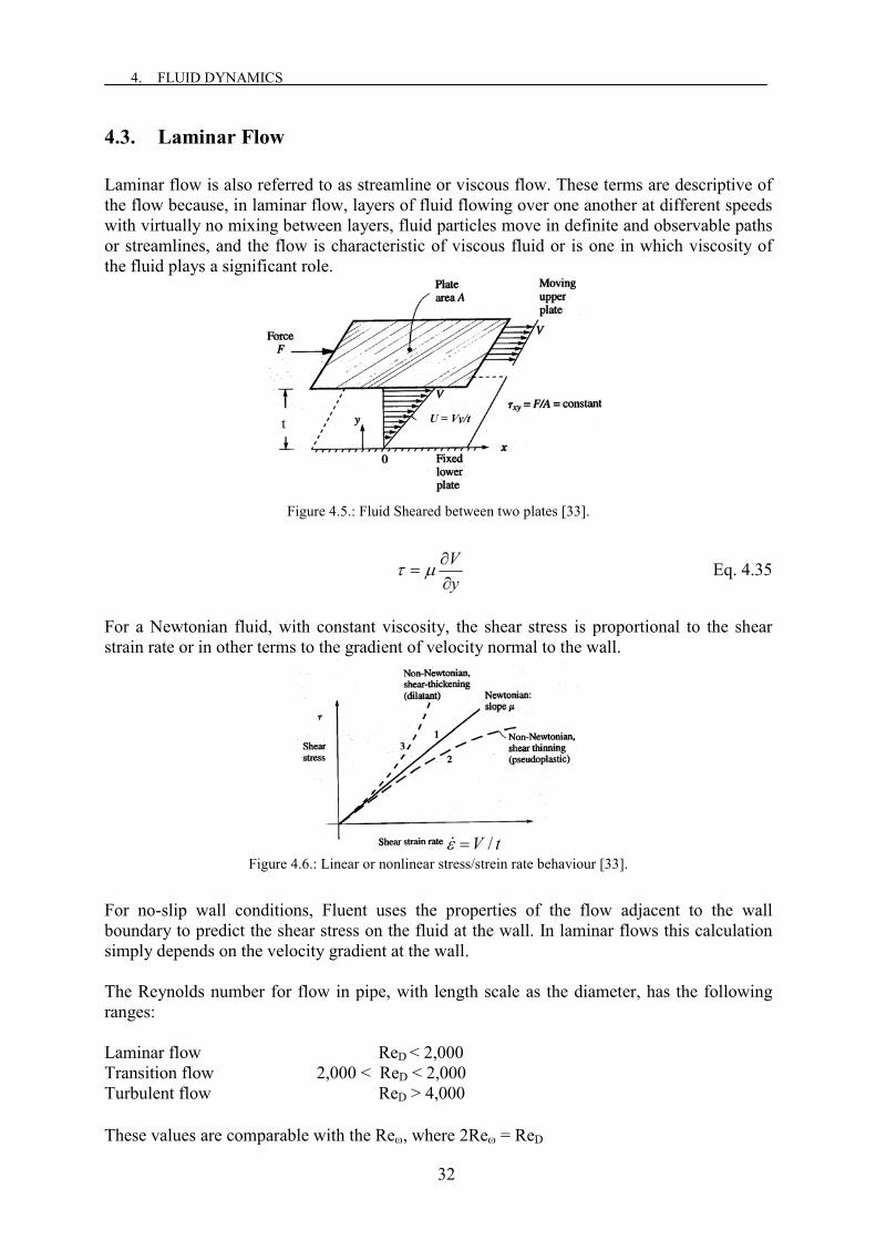
4. FLUID DYNAMICS
4.3. Laminar Flow Laminar flow is also referred to as streamline or viscous flow. These terms are descriptive of the flow because, in laminar flow, layers of fluid flowing over one another at different speeds with virtually no mixing between layers, fluid particles move in definite and observable paths or streamlines, and the flow is characteristic of viscous fluid or is one in which viscosity of the fluid plays a significant role.
t
For a Newtonian fluid,strain rate or in other ter
Figu
For no-slip wall condiboundary to predict thesimply depends on the v The Reynolds number franges: Laminar flow Transition flow Turbulent flow These values are compa
Figure 4.5.: Fluid Shea
��
with constant viscosms to the gradient of
re 4.6.: Linear or nonline
tions, Fluent uses t shear stress on the felocity gradient at th
or flow in pipe, with
ReD < 2,000 < ReD < ReD >
rable with the Re�, w
U = Vy/t
red between two plates [33].
yV�
�� Eq. 4.35
ity, the shear stress is proportional to the shear
velocity normal to the wall.
tV /���
ar stress/strein rate behaviour [33].
he properties of the flow adjacent to the wall luid at the wall. In laminar flows this calculation e wall.
length scale as the diameter, has the following
2,000 2,000 4,000
here 2Re� = ReD
32
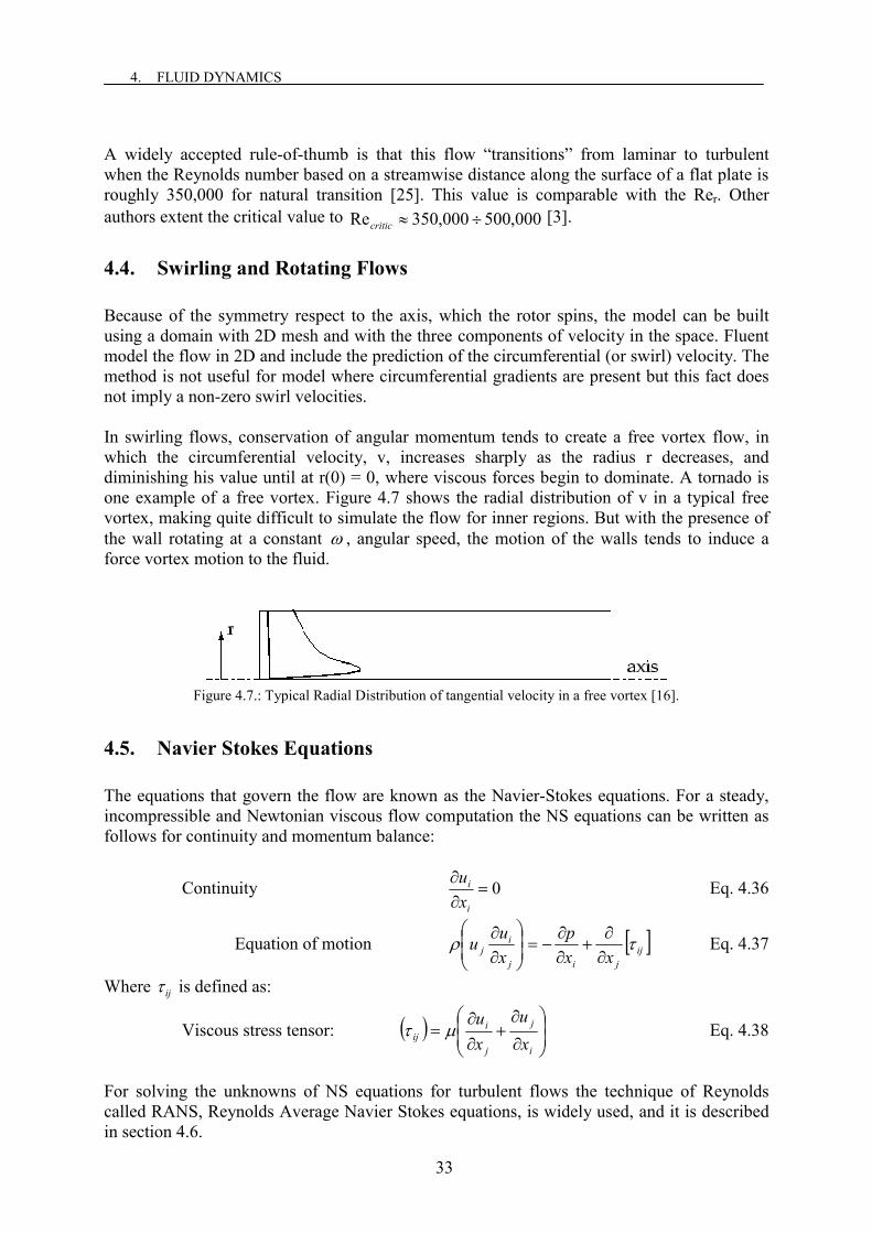
4. FLUID DYNAMICS
A widely accepted rule-of-thumb is that this flow “transitions” from laminar to turbulent when the Reynolds number based on a streamwise distance along the surface of a flat plate is roughly 350,000 for natural transition [25]. This value is comparable with the Rer. Other authors extent the critical value to 000,500000,350Re ��critic [3]. 4.4. Swirling and Rotating Flows Because of the symmetry respect to the axis, which the rotor spins, the model can be built using a domain with 2D mesh and with the three components of velocity in the space. Fluent model the flow in 2D and include the prediction of the circumferential (or swirl) velocity. The method is not useful for model where circumferential gradients are present but this fact does not imply a non-zero swirl velocities. In swirling flows, conservation of angular momentum tends to create a free vortex flow, in which the circumferential velocity, v, increases sharply as the radius r decreases, and diminishing his value until at r(0) = 0, where viscous forces begin to dominate. A tornado is one example of a free vortex. Figure 4.7 shows the radial distribution of v in a typical free vortex, making quite difficult to simulate the flow for inner regions. But with the presence of the wall rotating at a constant � , angular speed, the motion of the walls tends to induce a force vortex motion to the fluid.
Figure 4.7.: Typical Radial Distribution of tangential velocity in a free vortex [16].
4.5. Navier Stokes Equations The equations that govern the flow are known as the Navier-Stokes equations. For a steady, incompressible and Newtonian viscous flow computation the NS equations can be written as follows for continuity and momentum balance:
Continuity 0��
�
i
i
xu Eq. 4.36
Equation of motion � �ijjij
ij xx
pxuu ��
�
��
�
���
��
�
�
��
�
� Eq. 4.37
Where � is defined as: ij
Viscous stress tensor: � ���
�
�
��
�
�
�
��
�
�
i
j
j
iij x
uxu
�� Eq. 4.38
For solving the unknowns of NS equations for turbulent flows the technique of Reynolds called RANS, Reynolds Average Navier Stokes equations, is widely used, and it is described in section 4.6.
33

4. FLUID DYNAMICS
4.5.1. Momentum Conservation Equation for swirl Velocity The NS equations for 2D model can be reduce to one equation in the form of tangential momentum equation for 2D, swirling flow that is used by Fluent and can be written as:
ruv
rv
xr
rrxvr
xruv
rrvwr
xrv
t������ ��
�
���
��
��
�
�
�
����
���
�
�
�
�
��
�
��
�
��
�
� 32
11)(1)(1)( Eq. 4.39
where x is the axial coordinate, r is the radial coordinate, v is the swirl velocity, u is the radial velocity and w is the axial velocity. 4.6. Turbulence, The Reynolds–Averaged Equations The equations for stationary, incompressible and turbulent flow will be used. Turbulence is defined as an eddy-like state of fluid motion where the inertial-vortex forces are larger than any other forces that tend to damp them out. Turbulent flow is characterized by the rapid, and random fluctuations of field variables that lay over a more or less mean value due to the decay large instabilities. This fluctuation will affect the path of the particles travelling in irregular paths with no observable pattern and no definite layers. There is no definite frequency as there is in wave motion. (See Figure 4.12).
Figure 4.8.: Velocity fluctuation for turbulence Model.
Osborne Reynolds, in 1895, exploited this idea by defining every property u to the sum of a time-mean value u plus a fluctuation . u�
dtuT
uTt
t��
�0
0
1 Eq. 4.40
and the velocity field and pressure is
uuu ��� uvv ��� www ��� ppp ��� Eq. 4.41 In the present work was used the standard k-� turbulence model with near wall treatment. A comparison between the standard k-� turbulence model of Launder and Spalding and the low Re k-� model of Launder and Sharma (see Appendix A), was made for selecting the most suitable using the experimental results of Adams and Rice [2]. (See section 5.10). When Eq. 4.41 is applied in momentum equations, the tensor of Reynolds stress is symmetric, and appears six new unknown variables,
34

4. FLUID DYNAMICS
����
�
�
����
�
�
������
������
������
�
wwvwuwwvvvuvwuvuuu
tij� Eq. 4.42
The system has as unknowns the pressure and three components of velocity, plus the 6 new unknown stress gives a total of 10 unknowns with 4 equations, the continuity and three of impulse. For close the system is used Boussinesq assumption
Effective viscosity Eq. 4.43 te ��� ��
The Reynolds-stress terms uses the eddy viscosity from Boussinesq assumption:
� � iji
j
j
itji
tij k
xu
xuuu �����
32
���
�
�
��
�
�
�
�
�
���� Eq. 4.44
where � is the Kronecker delta function defined as: ij
ji
caseotherfor
ij���
�01
� Eq. 4.45
And k is the turbulent kinetic energy:
2wwvvuuk��������
� Eq. 4.46
And the dissipation rate of turbulent energy is formulated as:
��
�
�
��
�
�
��
����
jj
ii
xxuu
�� Eq. 4.47
Thus, the unknowns for the system is reduce to two unknowns and for closure the problem the standard turbulence k-� model of Launder and Spalding [21] is used in this investigation. Following the non-dimensional analysis, the closure equation can be founded as a function:
0),,( ��� kF t Eq. 4.48 Using the �-Theorem, the kinematic eddy viscosity is:
�
��
2kCt � Eq. 4.49
The model of k-� variables in the transport equations give in 3D case:
�
�
�
�
�
�
�
����
���
�
��
�
�
�
�
���
�
���
�
���
�
�
�
�
���
�
���
�
��
�
�
�
�
��
�
��
�
��
�
� Pzk
zyk
yxk
xzkw
ykv
xku
k
t
k
t
k
t Eq. 4.50
and
kCP
kC
zzyyxxzw
yv
xu ttt
2
21���
�
��
�
��
�
����
���
����
���
�
��
�
�
�
�
���
�
���
�
���
�
�
�
�
���
�
���
�
��
�
�
�
�
��
�
��
�
��
�
� Eq. 4.51
35

4. FLUID DYNAMICS
with the following empiric constants:
�C k� �
� 1C 2C 0.09 1.0 1.3 1.44 1.92 Table 4.2.: Constants of k-� model.
And the turbulent production rate is define in terms of average velocity
� �j
iji x
uuuP�
����� Eq. 4.52
in 3D case derivates to the form of:
��
���
��
���
��
���
�
��
�
���
��
�
��
�
����
���
�
��
�
��
��
�
�
��
�
��
��
�
����
���
�
���
��
�
��
222222
yw
zv
xw
zu
xv
yu
zw
yv
xuvP t Eq. 4.53
4.7. Transition Transition is not an easy issue, generally is treated as a 2D, steady phenomenon proceeding in the direction from laminar to turbulent, but it is actually much more complex; it is a stochastic, 3D, unsteady process which may proceed in either forward (laminar to turbulent) or reverse direction (turbulent to laminar). Roughly describing, transition is the intermediate flow between laminar and turbulent, the transition starts with some bursting process as depicts the Figure 4.9. The subsequent growth of the unstable waves and their breakdown into turbulence is not so well understood and a little detail of the actual process itself is known, but there have been many experiments and transition correlations.
Figure 4.9.: Bursting process in transition from laminar to turbulent [33].
Depending upon the case laminar or turbulent the friction factor will vary and different values of torque are expected as the shows, in a modification of the Moody diagram. The localization of the design point is with a very low Reynolds number in the laminar range, in order to have a high shear stress, or friction force over the walls of the disks.
36

4. FLUID DYNAMICS
Figure 4.10.: The flat plate Boundary layer (a) geometry with the boundary layer thickness and (b) typical shear
and heat flux distributions [33].
Furthermore, the real local Reynolds (not using the velocity of the wall) will be higher at the outlet than at the inlet, this is because the flow is accelerating (see Figure 5.33), due to the convergence of the geometrical configuration of the turbine, and at the inlet a process of laminarization are present because of thickening of the boundary layer and then transition from laminar to turbulent due to the fluid acceleration.
1 2 3 4 5
Figure 4.11.: Natural transition to turbulent over a flat plate [33].
37

4. FLUID DYNAMICS
4.7.1. Modes of Transition Mayle [25] present four important modes of transition: natural transition, bypass transition, separated flow transition and reverse transition (relaminarization). The first mode of transition depicted in Figure 4.11, which was first described by Tollmien and Schlichting (1979) [33], begins with a weak instability in the laminar boundary layer and proceeds to various stages (2-5) of amplified instabilities to fully turbulent flow. The second mode of transition is called bypass and it is caused by large disturbances in the external flow, bypassing the Tollmien-Schlichting (T/S) mode of instability, the first and second stage (see Figure 4.11) are completely bypassed. Mayle affirmed that the bypass mode is the common mode of transition in gas turbines engines. The third mode, separated flow transition does not occur in Tesla turbine since the flow is always accelerating due to the geometry of the rotor and separation of the boundary layer does not occur. In the Tesla turbine natural transition and bypass transition can take place, it strongly depends of the velocity of operation, roughly speaking, for lower speed natural transition would occur and for higher speeds the bypass transition mode is more common where only process of production, growth and convection of turbulent spots appears. 4.8. Relaminarization Transition from turbulent to laminar can arise with very strong acceleration [25] as it is found in the inner region of the rotor. Although little detail of the actual process itself is known, Mayle stated that the streamwise vortex associated with the turbulence in the boundary layer become greatly stretched as a result of the large acceleration and the dissipation of vorticity through the viscous effects. Relaminarization involves a balance between convection, production and dissipation of turbulent kinetic energy within the boundary layer. For evaluating the occurrence of relaminarization Mayle uses the acceleration parameter K defined by Schraub and Kline (1965), reported by Mayle [25] as:
dXdU
UK 2
�
� Eq. 4.54
and they settled that reverse transition can be expected to occur at low turbulence levels (TI < 5%) if the acceleration parameter is greater than 3x10⁻⁶ and as a result forward transition cannot take place if K is greater that K>3x10⁻⁶ . The acceleration parameter K represents the effect of free stream acceleration in the boundary layer. 4.9. Theory of Boundary Layer In Tesla turbine the effects of boundary layer are of main importance and through the boundary layer occurs all the change of energy. Figure 4.10 and Figure 4.11 depict the formation of a boundary layer near the leading edge of the boundary layer and its transition to turbulent. Fluid dynamic forces depend in a complex way on the viscosity of the fluid. As the fluid moves, the molecules right next to the surface stick to the surface. The molecules just above
38

4. FLUID DYNAMICS
the surface are slowed down in their collisions with the molecules sticking to the surface. These molecules in turn slow down the flow just above them. The farther one moves away from the surface, the fewer the collisions affected by the object surface. This creates a thin layer of fluid near the surface in which the velocity changes from zero at the surface to the free stream value away from the surface. This layer is what is called the boundary layer because it occurs on the boundary of the fluid. In reality, the effects of vortices and instabilities are three-dimensional.
Figure 4.12.: Schematic representation of laminar and turbulent boundary layer.
Boundary layers may be either laminar (layered), or turbulent (disordered) depending on the value of the Reynolds number. For lower Reynolds numbers, the boundary layer is laminar and the streamwise velocity changes uniformly in the direction away normal to the wall, as shown on the left side of the Figure 4.12. For higher Reynolds numbers, the boundary layer is turbulent and the streamwise velocity is characterized by unsteady swirling flows inside the boundary layer, as shown on the right side of the Figure 4.12. Besides Figure 4.12 shows the boundary layer thickness � and the displacement thickness of the boundary layer � , which its solution for a flat plate are due to Blausius and is defined in Eq. 4.55 and Eq. 4.56.
*
x
xRe
5�� with �
� xUx
�
�Re Eq. 4.55
��
��
0
* )(1 dyuUU
� Eq. 4.56
The plots showed in Figure 4.13 are only for laminar built up layer, they are plotted until the transitional Reynolds number.
39

4. FLUID DYNAMICS
Figure 4.13.: Plot of the boundary layer of the solution of Blausius for a flow over a flat plate.
For Figure 4.13 can be stated that with higher velocities the thickness of the boundary layer is lower, and the critical point (end of the line plot defined by the critical Reynolds of transition Rextr) starts nearer to the leading edge. Moreover the boundary layer for the air is thicker than for the water due to the fact that the air has a lower kinematic viscosity than the air. Generally, the thickness of a turbulent boundary layer is larger than that of a laminar boundary layer owing to the greater energy losses and mixing transports in the turbulent layer. At the outer region of the rotor of the turbine the local average velocity is lower than at the outlet, then formation or build up of boundary layer is present at the beginning, and transition to turbulent happens when the flow accelerates. In conclusion both laminar and turbulent boundary layers, with present of a core external flow (external to the boundary layer), are present inside the rotor of the turbine. The external flow reacts to the edge of the boundary layer just as it would to the physical surface of an object. The order of magnitude of all the terms in momentum equations at of order of magnitude equal to the thickness of the boundary layer because the region of external flow is minimum, and the boundary layer is in order of magnitude equal to the gaps between disks in the rotor of the turbine, then all the terms in NS equations have to be solved, and analytical exact solution does not exist for turbulent flow, so the most powerful tool nowadays is the CFD tool. However it is important to highlight that the tool is not so powerful for flows in transition region.
40

Chapter 5 5. Modeling in CFD and Results This section presents the following order: the results from laminar solution are presented in dimensional values and his corresponding similitude model in non-dimensional values. Next a comparison made between experiments and CFD is reported in order to select a suitable model for turbulence, and subsequent the results from turbulent simulation are documented. The entire rotor with 24 disks is simulated and its results are summarized. Finally, a 3D slide model is presented in which more features of the flow inside the turbine can be seen. 5.1. The Models and their Limitations A complete 3D model of the entire turbine with an acceptable grid resolution is not feasible due to restriction in time and computer resources. Then, incompressible flow is analyzed starting from a simple 2D model of one gap. This first turbine model, compound of one gap, does not allow for resisting torques acting in the turbine rotor, due to rotor-to-housing “disk friction”, bearings, seals, etc. Furthermore, the model ignores pressures losses that will occur in an actual turbine due to interference of the disk edges with the nozzle exit flow, due to irreversibility in the nozzle flow, and due to exit passage area changes and frictional losses. The final loss at the exhaust, may be actually be a gain, if the exit passage can be designed to produce a pressure recovery from the kinetic energy exhausting from the rotor, but the turbine model assumes no such recovery. To overcome some of the deficiencies of this model a second model was made and presented in section 5.12, which include the effects of the rotor-to-housing, and the outlet flow behaviour without the benefit of a pressure recovery device as an exhaust diffuser. Moreover, the two last models are not able to simulate the complete flow through the turbine, a last 3D model is proposed and solved with the presence of the nozzles, simulating one disk, (slide model) using periodic conditions, as it is used for cascades blades in conventional turbomachinery. The limitations of this model are that it does not take into account the presence of rotor-to-housing flow and the exhaust flow. Since the flow field is in transition regime the capabilities of CFD are limited, and both laminar solution and turbulent solution where performed for the initial models, and latter only the turbulent solution is obtained with the ground of the higher velocity obtained at the inner region of the rotor and the results extracted from section 5.10. Finally, another restriction is that for high velocities where the Tesla turbine claims higher efficiencies, the compressible effects became important, but this feature goes beyond the scope of the present work.
41

5. MODELING IN CFD AND RESULTS
5.2. Built of the Model The following general settings of the software and assumptions are consider into the CFD model:
Model Assumptions Settings Numeric Double Precision Space 2D Axisymmetric Swirl Time Steady-state flow Solver Segregated Energy Incompressible fluid Gravitational force is neglected Absolute reference frame
Discretization Scheme Variable Scheme Pressure PRESTO! Pressure Staggering Option Pressure-Velocity Coupling SIMPLE (Semi-Implicit Method for
Pressure-Linked Equations) Momentum Second Order Upwind Swirl Velocity Second Order Upwind For turbulent simulations k Second Order Upwind �� Second Order Upwind
Table 5.1.: General parameters used in Fluent.
5.3. Geometry The geometry was generated from the selected geometry of the turbine experimented by Rice [32]. This turbine was selected, because his performance parameters were reported and the author describes good behaviour after built two others similar turbines. An initial simple model is only the flow between the disks, very useful for a first approach.
Variables Non-dimensional Dimensional [mm] Outer Radius ro 200 101.6 Inner Radius ri 33 16.8 Width 1 0.508
Geometrical parameters ro/b 200 ro/ri 6.06
Table 5.2.: Geometry of domain.
The geometry is initially obtained from the patent of Nikola Tesla but modified by Rice in order to increase his performance. Nevertheless this geometry is not optimised as the same author accepts, there is not much technical literature that reports experimental results as it was made by Rice.
42

5. MODELING IN CFD AND RESULTS
Figure 5.1.: Geometry for CFD model, one gap model.
5.4. Restrictions of the Grid For an axisymmetric problem, the axis of rotation must be the x-axis and the grid must lie on or above the y = 0 line. In addition, it is required a sufficient resolution in the grid near the outlet region. Besides, rotating boundary layers may be very thin, and the Fluent model will require a very fine grid near a rotating wall. 5.5. Mesh The mesh and geometry was generated using GAMBIT 2.1.2, a software package of Fluent Inc. designed to pre-process the model for computational fluid dynamics (CFD), through its graphical user interface (GUI). Its basics steps are building, meshing, and assigning zone types to a model. The 2D structured mesh is used for an isolated rotor of the turbine, because of the simplicity of the geometry, and the advantage of a faster meshing and a faster solution. Besides, with Fluent it is possible to simulate the entire rotor in a 2D model grid using the capability of Fluent to handle 2D axysimmetric model with swirl, allowing to input the three components of the velocity in the space. The mesh used for laminar is showed in Figure 5.4 and it will be used the same mesh for the turbulent model with full resolution at the wall in order to apply near wall treatment instead of the commonly used wall functions for turbulence model that are no feasible because of the small gap of the fluid domain, as it can be seen in Figure 5.6. For an accurately solution at the vicinity of the wall, it is necessary a high resolution of the mesh for both solutions, for laminar, and for turbulent with near wall treatment. Therefore to
43
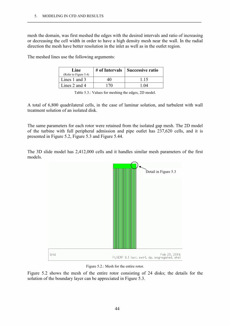
5. MODELING IN CFD AND RESULTS
mesh the domain, was first meshed the edges with the desired intervals and ratio of increasing or decreasing the cell width in order to have a high density mesh near the wall. In the radial direction the mesh have better resolution in the inlet as well as in the outlet region. The meshed lines use the following arguments:
Line (Refer to Figure 5.4)
# of Intervals Successive ratio
Lines 1 and 3 40 1.15 Lines 2 and 4 170 1.04
Table 5.3.: Values for meshing the edges, 2D model.
A total of 6,800 quadrilateral cells, in the case of laminar solution, and turbulent with wall treatment solution of an isolated disk.
The same parameters for each rotor were retained from the isolated gap mesh. The 2D model of the turbine with full peripheral admission and pipe outlet has 237,620 cells, and it is presented in Figure 5.2, Figure 5.3 and Figure 5.44.
The 3D slide model has 2,412,000 cells and it handles similar mesh parameters of the first models.
Detail in Figure 5.3
Figure 5.2.: Mesh for the entire rotor.
Figure 5.2 shows the mesh of the entire rotor consisting of 24 disks; the details for the solution of the boundary layer can be appreciated in Figure 5.3.
44

5. MODELING IN CFD AND RESULTS
Figure 5.3.: Detail of the mesh of Figure 5.2.
Figure 5.4.: 2D mesh for laminar and turbulent model with full resolution at the wall.
45

5. MODELING IN CFD AND RESULTS
In GAMBIT 2.1.2 there is the option of pre-setting the boundary conditions that will be used in Fluent (this boundary conditions can be modified also in Fluent); these boundary conditions are showed in Figure 5.4. One characteristic of quadrilateral/hexahedral cells that might make them more economical in this situation is that they permit a much larger aspect ratio than triangular/tetrahedral cells. A large aspect ratio in a triangular/tetrahedral cell will invariably affect the skewness of the cell, which is undesirable as it may impede accuracy and convergence. Therefore, for a relatively simple geometry as in the case of the Tesla turbine in which the flow conforms well to the shape of the geometry, it can be used a mesh of high-aspect-ratio quadrilateral/hexahedral cells. The mesh is likely to have far fewer cells than if you use triangular/tetrahedral cells. At the middle radius of the disks, the mesh presents the highest aspect ratio element with a value of 600, as it is showed in Figure 5.5, but because of the alignment of the flow with the grid using quadrilateral/hexahedral, this high aspect ratio is allowed.
Figure 5.5.: Mesh at the middle radius.
Some attempts of meshing the domain in order to use the wall functions for the standard k-� turbulence model were made but it showed not validity because of the thin gap of the configuration. Figure 5.6 shows this fact and some reasons are the high velocity, and also the small gap. The cell near the wall reaches to take almost 30 % of the domain, for a correct value of y+ > 30. With ��
�yuy ���
� . This would exhibit a wrong analysis because avoids the treatment near the wall.
46

5. MODELING IN CFD AND RESULTS
Figure 5.6.: Mesh for using wall functions in k-� turbulence model.
5.6. Convergence
Convergence as at first glance was no obtain when residuals were monitored, even with low values of residuals, first because the initial guess on the flow vas very near to the final solution a second the process is believed to be unsteady because the presence of transition phenomena. The criterion used for evaluating convergence was after reaching a value lower than 3 orders of magnitude 10-3, and one important quantity as the tangential at the outlet was monitor and verified that its value do not change anymore when increasing the number of iterations. Convergence was improved when the double precision characteristic of Fluent were used. The increase of a relaxation factor in Fluent means an acceleration of the convergence and the decreasing means a smaller value of the difference of a quantity. The residual of any variable computed by Fluent´s segregated solver is the imbalance in a cell, and can be interpreted as a type of mass generation or destruction. For this reason is also recommend by Fluent that the net mass imbalance between the inlet and outlet should be a small fraction lower than 0.5%. Settings for the solver controls:
Variable Relaxation factor Pressure 0.3 Density 1 Body Forces 1 Momentum 0.7 Swirl Velocity 0.9
Table 5.4.: Relaxation factors.
5.7. Working Fluid Properties
The fluid used for the dimensional simulation is air, with the following properties taken from [33]. Property for air @ 37 °C Symbol Value Units Viscosity � 1.9x10⁻⁵ smkg �
Density � 1.1387 3/ mkg Kinematic viscosity � 1.66856x10⁻⁵ sm 2 Reference pressure Pref 101325 Pa Enthalpy reference temperature Tref 273.15 K Specific heat capacity Cp 1.0052 kgKJ / Universal gas constant R 8314 kgmolKJ / Molecular weight M 28.97 kgmolkg / Constant of the air R/M 287 kgKJ /
Table 5.5.: Properties of working fluid.
47

5. MODELING IN CFD AND RESULTS
5.8. Boundary Conditions Inlet The inlet condition was specified with a velocity-inlet boundary, with a fixed value of velocity. For the inlet velocity is not necessary a profile because the gap is very thin compared to the area of the nozzle. For this model it is consider fully peripheral admission. For the turbulence simulations were selected a value of 5% of turbulence intensity, a mean value between a high and no presence of turbulence. Outlet The outlet condition was specified with a pressure-outlet boundary, with a gauge pressure value of 0. The reference pressure is set to ISO-conditions: Pa. 325,101�refp
Disks A no slip condition that means a value of zero relative velocity assigned to the wall. 5.9. Laminar Solution The solution presented in this section was taken from the post-processing of one of the seven simulations (those made to generated plot Figure 5.20). The case presented correspond to tangential velocity equal to 199 m/s (V=1.1).
Material Properties Dimensional Non-dimensional Density 1.1387 kg/m3 1 [-] Viscosity 1.9 x 10⁻⁵ kg/(ms) 1.9305 x 10⁻⁴ [-]
Boundary conditions Zones Value Value Inlet Velocity
Velocity Magnitude Radial component Tangential Component Axial Component
199.27 m/s 68,15 m/s 187,25 m/s 0
1.17 [-] -0.4 [-] 1.1 [-] 0 [-]
Outlet pressure p = 0 Pa P = 0 [-] Walls Rotation Speed of the disks
1675.2 m/s
0.005 [-], no slip condition
Table 5.6.: Data for laminar simulation.
The reference value of velocity is the outer tangential velocity of the disk. The Reynolds number Reb is 25.9. The velocity of sound is 2.07 times to the reference velocity. 5.9.1. Convergence of Laminar Solution For judging the convergence of the model is not only necessary to judge the values of the residuals plotted in Fluent, and showed in Figure 5.7, but also to monitor one of the solution parameters. In this case was selected the mass weighted average tangential velocity at the outlet and Figure 5.8 presents that his final value do not change after 150 iterations.
48

5. MODELING IN CFD AND RESULTS
Figure 5.7.: Convergence of laminar solution.
Figure 5.8.: Controling the convergence of swirl velocity at the outlet.
Characterization of the flow
Reynolds : 9.25Re2
�
�
�
�
� bb
, 180,5ReRe ���
���
��
bro
b�
The Reynolds number comparable to flow pipe is then 590,22 ��
Re , hence the flow is in the transition range.
-Mach 56.0352199
��M at inlet.
Surfaces integrals: Viscous moment: 0.14432 N-m
Viscous coefficient : 0.5474
Mass Flow Rate 0.02517 (kg/s)
Difference 4.27261x10⁻⁶ � 1.69x10⁻⁶ % Fluent [16] recommend at least < 0.5% as a parameter of controlling continuity and evaluating convergence.
49

5. MODELING IN CFD AND RESULTS
Mass Averaged Swirl Velocity at the outlet = 790.22 (m/s)
Mass-Weighted Average Total Pressure
pressure_outlet 576,541 (Pa)
velocity_inlet 676,479 (Pa)
Power for an isolated disk WTPshaft 8.241�� �
Using Euler is obtain the same value (for verification).
WVrVrmPshaft 4.241)7900168.01871016.0(675,1025167.0)( 2211 ����������
��
For n=24 disks HPWnPshaft 13.7318,5)1( ����
Efficiency %94.10��
��
�Pm
TP
mPshaft
�
� ��
�
�
5.9.2. Post-processing of the Laminar Solution The three components of velocity are presented in Figure 5.9, Figure 5.10, Figure 5.13 and Figure 5.14: velocity magnitude, radial, swirl (tangential) and the axial components. The post-processing of details of flow and profiles is made only for the case of tangential velocity, V= 187 [m/s] or V=1.1 [-].
Figure 5.9.: Velocity magnitude laminar solution, non-dimensional values.
From Figure 5.9 it is observed that the laminar solution presents a high acceleration of the fluid, nearly 5 times the inlet velocity. It can be understood that the tangential component of velocity will produce moment while the radial component of velocity will produce only losses.
50

5. MODELING IN CFD AND RESULTS
Figure 5.10.: Radial velocity, laminar solution, non-dimensional values.
The laminar velocity profile shows an inflection after the middle radius as it can be seen in Figure 5.11, and it agrees with the laminar solutions described by Matsch [24], which reports inflection at the inner region of the rotor. The inflection is also reported in literature in reference [51] for a pump case with Reb=20.
Figure 5.11.: Inflection of radial velocity for different radial stations, dimensional values.
This inflection appears after r=100 [-], 50.8 [mm], the middle inner region; the development of the inflection is shown in Figure 5.11. The inflection does not mean a reduction of velocity
51

5. MODELING IN CFD AND RESULTS
at the middle of the gap, but means different directions of the velocity vector as it can be seen in Figure 5.12.
-1400
-1200
-1000
-800
-600
-400
-200
0
0.000.050.100.150.200.250.300.350.400.450.500
200400
600800
10001200
1400
Rad
ial [
m/s
]
Gap [mm]
Tangential [m/s]
3D Graph Velocity Magnitude
Figure 5.12.: 3D plot of the velocity magnitude at the outlet of the rotor, dimensional values.
Figure 5.13.: Tangential velocity plotted with velocity magnitude.
Figure 5.13 depicts the tangential velocity compared to the total magnitude, it can be seen that the tangential velocity is predominant, where the two velocities are closed in values.
52

5. MODELING IN CFD AND RESULTS
Figure 5.14.: Axial velocity laminar solution, non-dimensional values.
A component of the axial velocity appears through the rotor, pronounced at the outlet and this can be explained with the thinning of the boundary layer due to the acceleration of the flow, with axial velocity in direction toward the walls (Figure 5.14). The axial profile describes also a symmetric behaviour.
Figure 5.15.: Total, dynamic and static pressure distribution along radius, laminar solution.
The total pressure at the middle plane (x=0.5), shows a small variance between inlet and outlet station, the total pressure difference increase near the wall, the plane X=0.05 is a value 5 % far away from the wall.
53

5. MODELING IN CFD AND RESULTS
Figure 5.16.: Total pressure for different radial station, laminar solution.
Figure 5.16 shows the variation of total pressure through the inlet to the outlet, this variation shows the region where energy is transferred by viscosity. Approximately 40% of the gap is used for effective transfer of the energy. If the stagnation pressure difference is very high, the efficiency is lower; these effects can be seen in the vicinity of the walls where the transfer of energy occurs. Further, it is concluded from these results that the gap can be reduced, for this geometry and at this regime of operation, in order to increased the efficiency.
Figure 5.17.: Variation of tangential wall shear stress along the radius, laminar and non-dimensional values.
The shear stress over the walls is finally the responsible of torque in the rotor, in Figure 5.17, this variable is plot and depicts a moment balance along all the rotor, at high values of radius low friction forces and a radius near the outlet high values of friction force showing a constant
54

5. MODELING IN CFD AND RESULTS
torque over the walls of the rotor. Once more it is concluded that the energy transfer and also the losses are higher at the inner region of the disks.
Figure 5.18.: Contours of stream functions at three radial stations.
The stream functions of the turbine are shown in Figure 5.18, in three radial stations; actually, there is not strong variations of streamlines but it can be appreciated a slightly variation at the middle of the rotor. Hence, it can be seen that closer are the streamlines to each other, higher is the velocity.
Figure 5.19.: Contours of axial velocity at inlet and outlet.
55

5. MODELING IN CFD AND RESULTS
As it is shown in Figure 5.19, the values of axial velocity are only significant in the inlet and outlet stations. For the inlet the formation of the boundary layer causes this behaviour. Another characteristic of the flow is that at the inlet with the build up of the boundary layer the axial velocity has the directions toward the centre and at the outlet toward the walls where the boundary layer is thinner due to the acceleration of the flow. The loading coefficient for an isolated disk is present in the Figure 5.20. In order to obtain this graphic, were performed seven simulations, with the same angular speed and increasing the mass flow (varying the inlet velocity, flow parameter), in order to simulate labs conditions of brake coupled to the turbine. In general, with higher mass flow the torque is higher in a linear relationship and the efficiency decrease with higher mass flow. The maximal efficiency is found at �=0.3 for V= 144 [m/s] or V=0.8 [-].
���Flow Parameter [-]
0.20 0.25 0.30 0.35 0.40 0.45 0.50
�Loading
Coefficient[-]
0.15
0.20
0.25
0.30
0.35
0.40
0.45
oU��
� �2orm
T
�
�
�
�
�
��
Figure 5.20.: Characteristic curve, loading coefficient., laminar solution.
Mass Flow [kg/s]
0.014 0.016 0.018 0.020 0.022 0.024 0.026 0.028 0.030 0.032
Power per disk[W]
50
100
150
200
250
300
350
Figure 5.21.: Characteristic curve, dimensional values.
For comparisons purposes with the results from Rice [32] and as a reference to compare with other machines, the dimensional values are presented for an isolated disk in Figure 5.21.
56

5. MODELING IN CFD AND RESULTS
The power output computed for the rotor of the turbine is simple the power per disks times the disks, for example for a mass flow of 0.03 kg/s is read a power per disk of, 350 W x 24 disks = 8,400 W; Rice [32] report values between 1 and 4 hp with efficiencies from 23% to 36%. These values are higher to those obtained by Rice [32] but these results are without the effects of the housing and nozzles. Efficiency of an isolated rotor; the high efficiencies expected by the one dimensional model presented by Nendl [27] presented in section 2.4 is not feasible due to the acceleration of the flow, the highest efficiency is obtained with lower mass flow.
���Flow Parameter [-]
0.20 0.25 0.30 0.35 0.40 0.45 0.50
Efficiency[%]
0
5
10
15
20
oU��
�
�
Totalo
shaf
pm
tP
��
�
Figure 5.22.: Efficiency of an isolated disk, laminar solution.
The lower efficiencies can be corroborated with the results from the theoretic model of Rice [32] showed in Figure 2.4. For the simulated turbine the parameter of flow rate and speed is
01256.03��rQ , and the value of 74.2�� oo Ur , which is the inverse of the flow
parameter. Following this, the efficiency will have values between 10% and 20% and it is achieved by laminar calculations.
���Flow Parameter [-]
0.20 0.25 0.30 0.35 0.40 0.45 0.50
Degree of
reaction[-]
0.75
0.80
0.85
0.90
0.95
1.00
o
rU�
�
��
1
21
21
1
PC
R�
�
�
Figure 5.23.: Degree of reaction for the laminar solution.
57

5. MODELING IN CFD AND RESULTS
Figure 5.23 shows that the Tesla turbine is a reaction type turbine with a high degree of reaction, contrary to the suggestion of Rice [32]. As it is known, highly impulse turbines have lower efficiencies. In addition the degree of reaction do not presents changes, with the variation of the flow parameter. Data obtain from Fluent:
Surface integrals, mass weighted average values V1
[m/s] U1
[m/s] V2
[m/s] V1* [-]
U1*=� [-]
U2 [m/s]
pt1 [Pa]
pt2 [Pa]
p1
[Pa] � [-]
� [%]
R [-]
119 43 524.14 0.7 0.2548 322 295784 243266 0.1896 0.189 11.90 0.9692136 49 586.58 0.8 0.2912 367 370265 308129 0.2288 0.228 12.13 0.9679153 56 651.8 0.9 0.3276 415 457939 384652 0.2653 0.265 11.93 0.9671170 62 719.45 1 0.3640 464 559303 473457 0.2995 0.299 11.49 0.9668187 68 790 1.1 0.4004 515 676479 576541 0.3308 0.330 10.94 0.9667204 74 860 1.2 0.4368 567 804184 689353 0.3626 0.362 10.39 0.9668221 80 933.68 1.3 0.4732 619 947961 816879 0.3909 0.390 9.83 0.9668
Table 5.7.: Summarize of performance of the turbine for laminar solution.
5.10. Comparison Results with Experiment for Selection of the Turbulence
Model
For the selection of the more suitable model was made a simulation of another geometry in order to compared it with the results of the experiment conducted by Adams and Rice [2], in which they reports the pressure difference field along an isolated rotor; the experimental fluid was chosen to be a water-ethylene glycol with a viscosity of 5 centistokes. This is useful because although the characteristic of the flow seems to have a low Reynolds number, the flow accelerates and the solution can change in the region of local high Reynolds number. The experiment of Adams and Rice [2] was required in order to confirm the initial results obtained by analytical and numerical solutions in [32, 24, 6, 5].
The comparison is made between the experiment data of Adams and Rice [2] and the laminar solution, the turbulent solution using the standard k-� with the standard empirical constants of Launder and Spalding [21] and with near wall treatment using high resolution near the wall, and finally with the low Re k-� variation model of Launder and Sharma [45] using viscous damping functions. Fluent uses the Launder and Sharma as default for low Re k-� simulations; the Launder and Sharma modification is presented in Appendix C. The target variable to compare is the static pressure difference because is reported by Adams and Rice, due to the facility to obtain its measurements from the experiments, in addition it can be related to the velocity field and Adams and Rice report its variation through the radial coordinate.
One issue that Adams and Rice [2] describe and accept is that for a big size the fluid flowing between the disks produces a turbine effect; however, for the single pairs of disks, insufficient torque is produced to maintain rotation in the presence on restraining torques incident to the experimental apparatus. And this fact reveals that this turbine is an impulse type one.
58

5. MODELING IN CFD AND RESULTS
Geometry of model is presented in Figure 5.24. The same boundary conditions of preliminary simulations were used.
Figure 5.24.: Geometry for the Adams experiment simulation.
The solution of model is also of interest because of the lack of experimental data reported in technical publications of the entire turbine. Through the comparison made with this simulation is validated on extension the calculation with CFD the simulation of the geometry used in this work. Settings: Reynolds Number Reb= 4.291 Radial Velocity Uo
*= -0.2338 [-] Tangential Velocity Vo
*= 0.7793 [-] Angle of the nozzle � = 16.7° [-] Viscosity [-] 0013655.0*
�vDensidad [-] 1*
��
Angular speed [-] 005859.0*��
The non-dimensional difference static pressure is defined as:
22*
orpp
��� Eq. 5.1
59

5. MODELING IN CFD AND RESULTS
Results and comparison for simulation of experiment of Adams and Rice:
r [-]0.0 0.2 0.4 0.6
Pressure Difference
[-]
0
2
4
6
8
10
EEEEEEEEEEEEEEEEEEEEEEEEEEEEEEEEEE
EEE
EEEEEE E E E E E E E E E E E E E E E E E E E E E E
Experimental Data from AdamsLaminar Incompres ibleTurbulent Lo Re k e IncompressibleTurbulent sk IncoE
� �2o
ist
rpp
��
[2]
�
Figure 5.25.: Comparison numerical solutions with experiment fr
These CFD results present good agreement with the experimeaccount that some degree of variation is obtained, because in thused. The experiment was design to provide full admission as numerical simulations is used the condition of fully admission in
60
s-�
mpressiblew-e�
0.8 1.0
E E E E E E E E E EEEEEEEEEEEEEEEEEEEEEEEEEEEEEEEEEEEEEEEEEEE
om Adams and Rice [2].
ntal but it must to take into e experiment 30 nozzles were nearly as possible, and in the the periphery.

5. MODELING IN CFD AND RESULTS
Figure 5.25 depicts the results of the comparison; as it can be seen the Low Re k-� model shows a strong variation in the inner part of the disks at the outlet, where the flow accelerates. It is easy to see that the low Re k-� do not work very good for the region that is called by the referenced literature as asymptotic region –called for flows with high Reynolds numbers–, where the local Reynolds is high and the solution present strong variation from the point at radius r=0.4 [-]. Furthermore, the real local Reynolds (not using the velocity of the wall, but the actual fluid velocity) will be higher at the outlet than at the inlet, this is because the flow is accelerating. Adams refers to it as the asymptotic flow in the inner region of the disks. Primary, for these reasons, the method of low Re k-� is not so useful and fails to achieved a good approach in the inner radius region on the flow field of pressure in comparison with the experimental data of Adams and Rice [2], and will be not used in the present investigation. The selected turbulent model is the standard model k-� with near wall treatment. To handle turbulent solution and option is allow in Fluent the near wall treatment, as it has been investigated by Haroutunian and Engelman [19], it is possible to simulate turbulence with high resolution near the wall, using the standard k-� model, controlling that the value of y+ for the first cell must be accomplished y+ < 5. 5.11. Turbulent Solution Hereinafter only non-dimensional cases are going to be threatened. The same parameters of laminar solution were used in turbulent case. Adding the following values, to turbulent conditions:
� �2
23 uk �� , � �2*
23 TIk � Eq. 5.2
where TI is the turbulence intensity defined as uu 2�
�TI , and the selected value is chosen
between low turbulence intensity and high turbulence intensity, TI = 5%.
mlkC
23
43
�� � , *
**
23
43
mlkC
�� � Eq. 5.3
where lm is the mixing small length scale defined as , and hm Dl �� 07.0 bDh 2�
Turbulence Value Units (Non-dimensional)
Kinetic energy k 0.00375 [-] Dissipation �� 2.6953x10⁻⁴ [-]
Table 5.8.: Turbulent boundary conditions at the inlet.
The turbulent boundary conditions at walls is k = � = 0, and at the outlet are the same that at the inlet for the computations when backflow happens.
61

5. MODELING IN CFD AND RESULTS
Figure 5.26.: Values of y+ for the cells adjacent to the walls.
Figure 5.26 depicts the values of y+ along the walls, in the radial coordinate are lower than 2.5 succeeding the rule of being lower than 5 to near wall treatment in standard k-� turbulence model.
Figure 5.27.: Velocity magnitude, turbulent case.
It is important to observe in Figure 5.27 the strong reduction of the higher value of velocity at the outlet in comparison to the laminar solution (see Figure 5.9); this difference of results can be interpreted as the type flow regime, between laminar and turbulent solutions, and furthermore shows the important roll of viscosity effects in the transition and turbulent regime.
62

5. MODELING IN CFD AND RESULTS
Figure 5.28.: Radial velocity, turbulent case.
The radial velocity do not present the inflection found in the laminar case; as it is showed Figure 5.28. The inflection does not mean a reduction velocity but indicates a change of direction of the velocity magnitude, this change is lower in turbulence case where the mixing and viscosity effects are higher and modifies the direction of the velocity vector; the higher value of effective viscosity compared to laminar can be the reason to this balance in the direction of the total and radial velocity. Figure 5.29 shows the tangential velocity profile for turbulent case.
Figure 5.29.: Tangential velocity, turbulent case.
63

5. MODELING IN CFD AND RESULTS
Figure 5.30.: Axial velocity, turbulent case.
The axial component depicted in Figure 5.30 presents different behaviour compared Figure 5.14 with stronger variation near the wall, in the boundary layer. The velocity normal to the wall increase with the present of the boundary layer; the higher value is observed at the outlet of the rotor. Comparison between laminar axial velocity (Figure 5.14) and turbulent axial profile gives a difference of ten times, because the components normal to the wall in the mixing length theory are trade by energy. The vector of the axial velocity in turbulent is also in the contrary direction than laminar, the direction of the vector point at the middle plane because of the thickening of the turbulent boundary layer; this occurs not in the laminar since there is no mass transfer in the normal direction to the wall. From here it is deduced the important roll that the axial velocity plays as a source of instabilities and the increment of the turbulence intensity as well as the drag over the disks.
Figure 5.31.: Plot of vectors in 2D plane.
64

5. MODELING IN CFD AND RESULTS
Figure 5.31 shows the vectors of velocity, in a 2D plane. It presents the low velocity presented at the inlet and higher in the inner region. The purpose of the plot is only for visualize the type of flow between two disks. For a better understanding of the real direction of the vectors of magnitude velocity see Figure 5.12.
Radius [-]
0.0 0.2 0.4 0.6 0.8 1.0
Velocity Magnitude
[-]
0
1
2
3
4
Velocity at the wallsVelocity in the mid-plane between the disks
Relative Velocity
Figure 5.32.: Velocity magnitude through radius, V*= 1.1, U*= -0.4.
With high velocities at the inner region, the losses are higher and the transfer of momentum through friction is higher. With the lower value of radius, the momentum is considered to be balanced. At some flow parameters the effect of ventilation appears, especially at low flow rates, with the rotational speed constant. About the Reynolds number The Reynolds number is calculated with the velocity at the wall at the entry, the velocity of the wall decreases, while the velocity of the fluid increases, there is not sense of speaking about the local Reynolds with the velocity of the wall, is more representative the local Reynolds with the computed velocity taken from CFD, then the asymptotic region is where the high velocities are present at the inner region of the rotor as it is showed in Figure 5.33. The critical Reynolds related to a plate Re=3x10⁵ is found at the middle radius with the velocity of the wall, where the radial velocity in laminar solution starts to present inflection of the profile. Therefore, problems of instabilities appear at the outer region when Standard k-� is used where there is a low local Reynolds and for the low Reynolds turbulence model, problems appear at the inner region as it is shown in Figure 5.25.
65

5. MODELING IN CFD AND RESULTS
Figure 5.33.: Plot of local Reynolds number along the radius, turbulent case.
Figure 5.34.: Total, dynamic and static pressure curve along the radius, turbulent case.
Figure 5.34 depicts the pressure curve along the radius, and comparing it to the laminar solution in Figure 5.15, can be concluded that the qualitative behaviour are the same but, the pressure level is lower for turbulent case, for which the efficiency is higher.
66

5. MODELING IN CFD AND RESULTS
Figure 5.35.: Flow angles values along the radius, turbulent case.
With the change of the angle � it is possible to view the change of direction of the path along the radius. Two plots were made in Figure 5.35, one in the middle of the disks on the other near the disks surface. The path of the fluid can be viewed as the change of velocity vector, through the radius. Moreover is also of interest to say that the path presents a smooth natural change of direction from 20° to 45° from inlet to outlet, the difference of values, depicts in Figure 5.35 between a curve at the disk plane and a plane at the middle of the gap, explains the existences of different paths in the space for a particle of fluid.
���Flow Parameter [-]
0.20 0.25 0.30 0.35 0.40 0.45 0.50
�Loading
Coefficient[-]
0.3
0.4
0.5
0.6
0.7
0.8
0.9
oU��
� �2orm
T
�
�
�
�
�
��
Figure 5.36.: Loading coefficient for turbulent solution, isolated disk.
67

5. MODELING IN CFD AND RESULTS
The values of Figure 5.36 are higher for turbulent solution, nearly two times compared with laminar case showed in Figure 5.20.
���Flow Parameter [-]
0.20 0.25 0.30 0.35 0.40 0.45 0.50
Efficiency[%]
0
5
10
15
20
oU��
�
�
Totalo
shaf
pm
tP
��
�
Figure 5.37.: Efficiency for turbulent solution, isolated disk.
The efficiency showed in Figure 5.37 is also higher for turbulent case that those from laminar solution (compared with Figure 5.22).
Flow Parameter0.20 0.25 0.30 0.35 0.40 0.45 0.50
RDegree of Reaction
0.5
0.6
0.7
0.8
0.9
1.0
flow parameter vs R laminar Analytical Model flow parameter vs R turbulent
o
o
rU�
�
��
shshshR
������
����
Figure 5.38.: Degree of reaction for turbulent solution in comparison with laminar solution, isolated disk.
The analytical model made to reach the Eq. 4.34, with bulk parameters for the characteristics curves as Rice [32] used, were developed using the assumption that the tangential velocity remains constant through the radius, which makes the model weak, but can proportionate us a good point of qualitative comparison. This assumption have the ground that in the Tesla turbine, contrary to conventional turbomachinery, the angle at the outlet of stage - the relative outlet angle of an airfoil- is not known from the geometry due to the natural path of the flow through the disks. The others curves using this analytical model, such loading coefficient and efficiency are qualitative useful but not numerically.
68

5. MODELING IN CFD AND RESULTS
Figure 5.39.: Contours of pressure at the outlet of the gap.
From Figure 5.39 can be seen that the total pressure is lower at the walls where the dynamic head is zero, and is higher at the middle of the gap, a better reference for this graph is the plot show in Figure 5.16. The change of total pressure is accomplished near the wall in the boundary layer region, where the energy transfer occurs.
V1* U1*=� V2* pt1* pt2* p1* � � [%] R 0.7 0.2548 1.884 5.263 3.057 4.986 0.3886 17.62 0.947 0.8 0.2912 2.029 6.324 3.726 5.962 0.4646 17.88 0.943 0.9 0.3276 2.175 7.51 4.468 7.051 0.5405 17.77 0.939 1 0.3640 2.3218 8.811 5.281 8.245 0.6164 17.46 0.936 1.1 0.4004 2.4662 10.211 6.156 9.526 0.6926 17.08 0.933 1.2 0.4368 2.611 11.742 7.118 10.927 0.7685 16.62 0.931 1.3 0.4732 2.7558 13.368 8.141 12.411 0.8448 16.16 0.928
Table 5.9:. Summarize of performance of the turbine for turbulent solution.
Figure 5.40, Figure 5.41 and Figure 5.42 show the differences between the laminar and turbulent solution, for each type of pressure.
69

5. MODELING IN CFD AND RESULTS
Radius [-]20 40 60 80 100 120 140 160 180 200
Pressure [-]
0
5
10
15
20Dynamic pressure turbulentDynamic pressure laminar
Figure 5.40.: Dynamic pressure through the radius.
Radius [-]20 40 60 80 100 120 140 160 180 200
Pressure [-]
0
5
10
15
20
Static pressure turbulentStatic pressure laminar
Figure 5.41.: Static pressure through the radius.
The big differences between the two models, give us an idea about the difficulties of modelling such flows using CFD and these problems is also explained with the suddenly change in the Moody diagram between laminar and turbulent, in transition regime (See Figure 4.10).
70

5. MODELING IN CFD AND RESULTS
Radius [-]20 40 60 80 100 120 140 160 180 200
Pressure [-]
0
5
10
15
20
radius vs total_pr_turb radius vs total_pr_lam
Figure 5.42.: Total pressure through the radius.
5.11.1. Numerical Characterization of the Relaminarization The relaminarization can be predicted using the theory proposed by Mayle [25] and presented in section 4.8; the radial distance at which relaminarization occurs can be extracted from Figure 5.43. The two solutions are very similar in the outer region, but for a lower radius in the asymptotic regions the two solutions show different tendency.
Radius [-]40 60 80 100 120 140 160 180 200
Acceleration Parameter K=�/U2(dU/dx)
[-]
-5e-5
-4e-5
-3e-5
-2e-5
-1e-5
0
1e-5Upper Specification
TurbulentLaminarUpper Specification
Schraub and Kline (1965)
Reverse transition
Beginning of reverse transition (Relaminarization)
K= -3e-6
Figure 5.43.: Distribution of the acceleration parameter for the radial flow between disks.
For both cases laminar and turbulent the relaminarization takes place at a radius of 110, at 55% of radial distance to the outlet radius; approximately the same region where laminar
71

5. MODELING IN CFD AND RESULTS
solution becomes inflected, see Figure 5.11. Further, it is also visible the strong acceleration presented at the outlet. 5.12. Simulation of the Turbine with Full Peripheral Admission. For this simulation the same parameters of the isolated gap turbulent simulation were retained, for the grid as well as for the boundary conditions. It was solved using 2D axysimmetric solver of Fluent with one plane of symmetry to obtain the entire rotor of 24 disks. Figure 5.44 depicts the entire turbine but the model is composed of only one quadrant using axisymmetry and one plane of symmetry. The outlet is fixed for both sides, simply with a pipe. At the outlet there is no diffuser. Change of direction takes place with a change of area, which works as a nozzle. This model is useful in order to observe the effects due to the outlet of the turbine and the lateral sides of the housing.
Detail in Figure 5.50
Figure 5.44. 2D model of the turbine with full peripheral admission.
The outlet is characterized by high swirling flows with two regions of recirculation, as it can be seen in Figure 5.56. The extension of the outlet was extended in order to assure a flow without backflow.
72

5. MODELING IN CFD AND RESULTS
The convergence history of residuals and static pressure at the outlet are depicted in Figure 5.45 and Figure 5.46, characteristic curves for the turbine and plots with qualitative behaviour of the flow are presented from Figure 5.52 to Figure 5.62.
Figure 5.45.: Convergence of 2D turbine model.
Figure 5.46.: Convergence history of static presssure for 2D turbine model.
73

5. MODELING IN CFD AND RESULTS
Flow Parameter ����]
0.20 0.25 0.30 0.35 0.40 0.45 0.50
� Loading
Coefficient[-]
0.3
0.4
0.5
0.6
0.7
0.8
0.9
Figure 5.47.: Loading coefficient for turbulent solution, turbine.
Figure 5.47 shows the results for the Tesla rotor and they are very close to that obtained in one gap as it is shown in Figure 5.36. The power is not strong affected by the presence of the
outlet, or the presence of the lateral static walls of the housing.
Flow Parameter �����
0.20 0.25 0.30 0.35 0.40 0.45 0.50
� Efficiency
[%]
0
5
10
15
20
flow parameter vs efficiency_rotor flow parameter vs efficiency_57
Figure 5.48.: Efficiency for turbulent solution, turbine.
The method of computing the efficiency reveals the change of the properties at the outlet of the turbine; the plane 57 is localized in the pipe at a distance downstream from the symmetry
74

5. MODELING IN CFD AND RESULTS
plane of 57. Nevertheless the loading coefficient is not affected, it is concluded that the effects, at the outlet is reduced in approximately 6 points in the efficiency, due to the viscosity losses caused by the change of direction, change of area, highly rotating swirl flow and recirculation as well as the losses at the trailing edge.
Flow Parameter
0.20 0.25 0.30 0.35 0.40 0.45 0.50
R Degree of reaction
[-]
0.5
0.6
0.7
0.8
0.9
1.0
Figure 5.49.: Degree of reaction for turbulent solution, turbine.
Surface integrals, mass weighted average values V1* U1*=� V2* U2* pt1* pt2* p1* � � R
0.7 0.2548 1.790 1.6 9.59 7.16 9.31 0.3828 15.75% 0.974 0.8 0.2912 1.933 1.84 11.62 8.73 11.26 0.4631 16.02% 0.972 0.9 0.3276 2.076 2.06 13.71 10.32 13.25 0.5436 16.04% 0.969 1 0.3640 2.220 2.29 15.89 11.96 15.32 0.6239 15.88% 0.967 1.1 0.4004 2.360 2.51 18.38 13.87 17.69 0.7041 15.61% 0.966 1.2 0.4368 2.500 2.74 21.05 15.91 20.23 0.7835 15.24% 0.965 1.3 0.4732 2.643 2.97 23.93 18.13 22.97 0.8636 14.89% 0.963
Table 5.10.. Summarize of performance of the turbine for turbulence solution.
75

5. MODELING IN CFD AND RESULTS
Figure 5.50.: Detail of the grid.
The values y+ were checked and the grid was adapted in order to have values lower than 5 for y+ near the walls. This value is monitored and presented in Figure 5.51.
Figure 5.51.: Values for y+ along the housing wall.
76

5. MODELING IN CFD AND RESULTS
Figure 5.52.: Plot of vector of velocities at the trailing edge.
From Figure 5.52 to Figure 5.60 can be appreciated some visualizations and details of the flow, vectors of velocity and zones of recirculation which increase the losses of the turbine, especially the increment due to the losses at the leading edge, trailing edge and at the outlet.
Figure 5.53.: Plot of vector of velocities at the leading edge.
77

5. MODELING IN CFD AND RESULTS
Figure 5.54.: Plot of vector of velocities at the leading edge, detail at last disk.
Figure 5.55.: Plot of vector of velocities at the outlet of the rotor.
In Figure 5.55 and Figure 5.60 is it visible the effects of the trailing edge of the disks, where eddies are presented. These effects with the zone of recirculation increase the losses at the outlet of the turbine.
78

5. MODELING IN CFD AND RESULTS
Figure 5.56.: Plot of vector of velocities at the center of the turbine.
Figure 5.57.: Path lines along the turbine.
Figure 5.57 shows the path lines along the turbines, especially the behaviour at the outlet of the turbine, showing the highly swirling component near the axis, where zones of recirculation come into sight, effect that continues through the outlet until the exhaust.
79

5. MODELING IN CFD AND RESULTS
Figure 5.58:. Detail of path lines at the leading edge, the plot shows the half of the rotor.
Figure 5.58 presents details of the flow at the leading edge of the rotor. The leading edge of the rotor can be improved, to handle an smoother entry of the flow to the rotor.
Figure 5.59.: Detail of path lines at the leading edge between two disks.
Figure 5.59 shows a detail of the plot of Figure 5.58. The velocity increase nearly to the double at the inlet of the rotor.
80

5. MODELING IN CFD AND RESULTS
Figure 5.60.: Detail of path lines at the trailing edge.
The zones where there are no path lines (Figure 5.60), are zones of recirculation, also the lower pressure is found in the zones of recirculation (see Figure 5.61 and Figure 5.62).
Figure 5.61.: Contours of pressure for the Tesla turbine.
81

5. MODELING IN CFD AND RESULTS
Figure 5.62.: Details of contours of pressure for the Tesla turbine at the outle of the rotor.
5.13. 3D Slide Model, Simulation and Results
For the 3D simulation the inlet nozzles were added to the rotor at an angle �� 20� ; two nozzles were disposed in opposite diametric points as it was made in the experiments of Rice [32]. A complete simulation of the turbine with the 24 disks of the rotor, the inlet nozzles and the outlet is prohibited and restricted by the computational resources. Therefore, a model of one slide of the turbine, containing a single disk, with periodic conditions at both lateral sides, was simulated. Figure 5.63 presents the geometry of the model, the model do not consider the effects of the outlet.
Figure 5.63.: Side view of one slide for the tesla turbine.
82

5. MODELING IN CFD AND RESULTS
For meshing the volume, the domain was divided in 16 volume regions, with the purpose of meshing each edge controlling its parameters in order to get a similar grid as the one used in 2D simulations. These volumes are depicts in Figure 5.64. The finite volumes used were hexahedral using the mapped scheme. A slide gives a total of 2,412,000 cells and one iteration takes 3 minutes, a solution with good convergence was found to be at 5,000 iterations (see Figure 5.69), were some of the instabilities of the axial velocity disappears, and it takes more or less fourteen days.
7
8
1 1
3
6
2
5
4
Figure 5.64.: 3D plot of the domain with subdivisions in smaller volumes.
The grid used is presented in Figure 5.65 to Figure 5.68. The disk is in the middle of the domain with two regions at each side that conformed the gap, the axial distance is not in scale in Figure 5.64. This model includes the effects of the presence of the nozzles, and effects due to interaction with the housing, but the effects due to the outlet and due to the housing at the lateral faces, cannot be simulated by this model, due to geometrical restrictions using periodic conditions.
83

5. MODELING IN CFD AND RESULTS
Figure 5.65.: Mesh for the 3D slide model.
Figure 5.66.: Detail of the mesh at the nozzle
In Figure 5.66 is visible the mesh of the gap between the rotor and the housing. The non-dimensionless radius of the housing is 204 [-].
84

5. MODELING IN CFD AND RESULTS
Figure 5.67.: Detail of the mesh at the outlet.
In Figure 5.67 and Figure 5.65 can be seen the high resolution of the mesh obtained at the outlet for an appropriated mesh at the outer radius, and very useful for the high velocities presented at the inner region.
Figure 5.68.: Detail of the mesh of the disk.
Figure 5.68 shows the high resolution used near the vicinity to the walls of the disk, with the aim of obtaining an appropriated solution of the equations near the wall.
85

5. MODELING IN CFD AND RESULTS
5.13.1. Setting up of 3D slide model The geometrical values for the mesh used in this model are nearly to those used in 2D models (Table 5.3) and they are showed in Table 5.11. The geometry of the nozzle is settled by the � angle and the area. The area of one nozzle is 80 [-], the width is 2 [-] the gap ant the disk with the same spacing, and in dimensional case for the turbine of Rice, would represent a pipe with diameter of 1½ in; the nozzle has a convergence angle of 1.5° degrees.
Line (Refer to Figure 5.64)
# of Intervals Successive ratio Line 1 20 1.1 Line 2 40 1.04 Line 3 150 1 Line 4 10 1 Line 5 170 1.01 Line 6 125 1 Line 7 125 1 Line 8 16 1
Table 5.11.: Values for meshing the edges, 3D model.
5.13.2. Boundary conditions The new boundaries conditions included are the periodic ones. The others are the same of the last models; the housing is a wall with condition of no slip. Periodic boundary condition: The face of each side is physically connected to the another lateral face, and this is feasible due to the symmetry of the flow in the middle of the gap, without any pressure drop across the periodic planes. Periodic boundary conditions are used when the physical geometry of interest and the expected pattern of the flow solution have a periodically repeating nature; in this case can be simulated one disk, an extent the solution for an infinite number of disks in the axial direction. The model uses conformal periodic boundaries, in which the periodic zones must have identical grids. The conformal periodic boundaries can be created in GAMBIT when the volume mesh is generated. Symmetry planes are not possible due to the presence of nozzles. Inlet velocity boundary condition: The velocities at the inlet of the nozzle were chosen with the purpose of generate approximately the same mass flow as those obtained in 2D simulations, the values are shown in Table 5.12. With the presence of the nozzle the values of inlets velocities are nearly 3 times comparing to the full peripheral admission of 2D models.
86

5. MODELING IN CFD AND RESULTS
Velocity inlet conditions for the nozzle V Dimensionless velocity
0.7 2 0.8 2.29 0.9 2.57 1.0 2.85 1.1 3.14 1.2 3.43 1.3 3.71
Table 5.12.: Velocity inlet values for the nozzle.
5.13.3. Convergence The convergence in the initial iterations shows good behaviour but integral parameters, as the outlet velocity mass weighted average value and static pressure at the inlet still continues changing at 1,000 iterations; later the instabilities of the component of axial velocity appear and the torque continue increasing (the turbulence viscosity increases with the increase of turbulence in the normal direction to the wall), after 5,000 iterations the integrals parameter do not change anymore and the higher residual stabilizes near a value in order of magnitude of 1x10⁻⁵.
Figure 5.69.: Convergence history of residuals.
In Figure 5.69 can be noticed that the instabilities of residuals is due to the axial velocity and affects the residuals of the continuity. The instabilities give evidence of the difficulties of the model to converge fast.
87

5. MODELING IN CFD AND RESULTS
Iterations0 1000 2000 3000 4000 5000
Velo
city
Mag
nitu
de o
n pr
essu
re_o
utle
t.2
0
1
2
3
4
5
Figure 5.70.: Convergence history of velocity magnitude.
Even though the velocity magnitude do not change beyond 2,000 iterations, the torque will stabilize after 3,000 iterations (see Figure 5.70), where some instabilities appear, then it was necessary to observe if this instabilities will increase or decrease; finally they decrease until, as sometimes is referred, the convergence at the level of machine accuracy, which is a good indicator of convergence when the residuals flatten as it happens at the end of the plot (of residual value vs. iteration Figure 5.69). 5.13.4. Results This model is not exactly comparable with the 2D models. The presence of nozzles makes it different, but gives a closer approximation of what happens inside the Tesla turbine. The post-processing was made for the case of tangential velocity of 1.3 [-]. The torque increases significantly, with the presence of the nozzle in comparison to 2D simulations, as it is visible in Figure 5.71, due to the high velocity at the nozzles and higher turbulence at the leading edge.
���Flow Parameter [-]
0.20 0.25 0.30 0.35 0.40 0.45 0.50
�Loading
Coefficient[-]
1.6
1.8
2.0
2.2
2.4
2.6
2.8
3.0
Figure 5.71.: Loading coefficient for 3D slide model.
88

5. MODELING IN CFD AND RESULTS
���Flow Parameter [-]
0.20 0.25 0.30 0.35 0.40 0.45 0.50
Efficiency[%]
0
5
10
15
20
25
Figure 5.72.: Efficiency of 3D slide model
Figure 5.72 presents the efficiency of the turbine when it is simulated with the nozzles, it is seen that for lower mass flow the efficiency increase more sensible that for the simulation of the rotor (see Figure 5.37).
Figure 5.73.: Path lines colored by velocity magnitude.
The path lines is one of the most useful plots to visualize the flow patterns, and what makes CFD a cheaper and powerful tool in contrast to the expensive costs of experimental installation requirements, the particle path lines presented are absolute. They present regions where the disks act as a brake especially near the nozzles, where some recirculation zones take place, these phenomena are called by literature as ventilation problems. The regions where the path lines are near to each other indicate a high velocity, and can be appreciated in Figure 5.73; (not all the path lines are plotted). In addition, the plot of Figure
89

5. MODELING IN CFD AND RESULTS
5.73 give evidence that the paths of the spiral are short and do not flow in many circular paths as it was suggested by Tesla and reported by Rhetta [31].
Figure 5.74.: Contours of total pressure at the surface of the disks.
In Figure 5.74 the contours of total pressure are plotted with a maximum value of 30.9 at the inlet of the nozzle, value that is higher in comparison with the 2D case (see Figure 5.42). This is caused by the presence of the nozzles with higher velocities, besides it can be seen that the pressure is axysimmetric presenting concentric values after the first third of the radius, before this point the disturbances of the nozzles cause non-symmetry.
Figure 5.75.: Contours of total pressure at the middle of the gap.
90

5. MODELING IN CFD AND RESULTS
For the total pressure at the middle of the gap (Figure 5.75), the distortion of the pressure field is higher than at the disk and the pressure is concentric after the middle section of the radius.
Figure 5.76.: Contours of total pressure at leading edge in the middle of the rotor.
In Figure 5.76 can be appreciated an increment of the total pressure in the leading edge, where the area reduces to the half, due to the contribution of the axial component., when it changes its vector direction.
Figure 5.77.: Vectors of velocity magnitude and total pressure contours at the middle of the gap.
91

5. MODELING IN CFD AND RESULTS
The flow field of velocities presented in Figure 5.77 shows high values in the zones after the nozzles and at the outlet of the rotor, and some regions of low velocity, particularly near the housing and in the rotor before the flow entry to the rotor through the nozzles.
Figure 5.78.: Detail of vectors of velocity magnitude near the wall of the housing.
The profile near the neighborhood of the housing is visible in Figure 5.78, where the condition of no slip is satisfied, the vector velocities at the gap between the rotor and the housing is between the range 4.09x10⁻¹ to 8.18 x10⁻¹, which indicates that the flow is acting as a brake in 75% of the periphery of the disks, only nearly after the nozzle the velocity is higher than the velocity of the disk.
Figure 5.79.: Veloctiy magnitude, through the radius.
The gradual change of the direction of velocity is plotted in Figure 5.79, it proves the idea of
92

5. MODELING IN CFD AND RESULTS
Tesla that the changes in velocity and direction of movement of the fluid should be as gradual as possible (see section 2.1), and furthermore, with the presence of the nozzle the assumption of constant tangential velocity used for obtaining Eq. 4.34, is not far away from reality.
Figure 5.80.: Contours of axial velocity at the middle of the gap.
The origin of the axial velocity component is found at the leading edge. At outlet of the rotor it is very high and has opposite directions, the acceleration behaviour is also visible in Figure 5.43.
Figure 5.81.: Wall shear stress over the disk.
The wall shear stress shows the regions where the field flow produces torque, in this case the transfer of energy is high after the nozzles and at the inner region of the rotor. The low wall shear stress showed at the outer region of the rotor is compensated with the radial distance giving a similar torque as in the inner region. The gap between the rotor and the housing as well as the aft region near the nozzle work as brakes zones.
In the 3D model, more flow features and visualizations of the flow inside the turbine was depicted, with the purpose of showing more qualitative characteristics of the flow.
93

Chapter 6 6. Discussion and Conclusions 6.1. Discussion The flow in the Tesla turbine was simulated with different geometrical models, as well as laminar and turbulent approach. Since the flow itself is found in a transition regime with multiple processes -as transition, relaminarization, recirculation, between other phenomena- an exact simulation that full fills all the physical requirements is quite difficult to achieve with CFD tool. Nevertheless both approximations are valid and they would show different features, characteristics and behaviour typical for each case and in extension for the Tesla turbine. One of these differences is that the inflection point of radial velocity profile presented in laminar solution disappears in the turbulence model, for which the turbulent effects act as a mechanism of balanced in the axial direction. In contrast, experimental research cannot measured velocities profiles, only static pressure as it was reported by Adams and Rice [2], due to the gap between disks is very thin; CFD provide solution to this problem and furthermore to micro turbines. Generally, there is a lack of reports of experimental works; for this analysis the geometry selected from Rice [32] to perform the simulations was not possible to compared with the experimental data because of omitted data in the reported experiment, but good agreement was found between the models and the experimental results of Adams and Rice [2]. In this last comparison, it is visible that turbulent approach describes better the flow inside the turbine for this geometry and operation point. Besides, the field of static pressure and his corresponding velocity field show good agreement with experimental results. Separately from transition problems, the flow has also high swirling velocity components with significant gradients of acceleration at the inner region of the rotor, which make the solution more complicated to solve and need extra iterations in order to achieve a good convergence solution. Convergence is an important issue in CFD because of the iterative nature of the solution, and it can give evidence of a well posed model indicating some physical facts, for example a turbulent flow will not convergence easily with a laminar approach or vice versa. Simulation with very low flow coefficients do not show convergence because physically the flow would go in outward radial direction and the turbine would work a with big zones of ventilation when the angular speed is maintain constant. Additionally, there is no unification of the Reynolds number and dimensionless number presented by several researches. The numbers reported in this work can be compared with flow pipe theory (Re�), or with flow over a flat plate (Rer). Therefore, the three Reynolds numbers (Reb, Rer, Re�) are creditable and they present the same features of the flow from different points of references. The Reb is the most known by authors on this topic (and not comparable with theoretical models), and reflects also the same behaviour of transition of regime as it is described in section 2.3, showing that when the gap is reduced the flow will become laminar. Besides, the Reynolds characterizes the flow at the inlet, it varies through the rotor what makes difficult to simulate in transition regime.
94

6. CONCLUSIONS AND DISKUSSION
The results show that multiple disk turbines are workable and feasible, in the engineering sense, but they present a low efficiency in both laminar and turbulent cases; lower for laminar case; the difference between these cases is significant. A good parameter for evaluating the performance of the Tesla turbine is the loading coefficient, which reflects the amount of torque obtained from the turbine. It is noticeable that for turbulent case the amount of torque is higher, nearly the double, for which the total viscosity is higher with the present of the turbulent viscosity. The concept used for evaluating efficiency was the total-to-total efficiency. The 2D model present that the efficiency of the rotor is not as high as it is suggested by literature. Moreover, the results of 3D slide model shows that losses due to the presence of the nozzles are not very high as reported in literature and for low mass flow the efficiency increases in comparison with the model wit out nozzles. Rice [32] anticipate to this results with his analytical solution presented in Figure 2.4, indicating low efficiencies for common operation points, for which the mass flow is high. The efficiencies are similar in the three models. The machine is feasible for a low range of power where the efficiency of conventional turbomachinery is not very high and it can handle working fluid with particles, contaminants and high viscosity. Bigger turbines are not feasible for this kind of machines and they are not worthy of further investigation. In the Moody diagram (Figure 4.10) can be see also that if the Reynolds is number reduced the laminar regime would show a higher wall shear stress. With higher turbulence levels the transfer of energy is higher due to the drag is higher, similarly the torque increase and present higher efficiency even though the losses are higher for turbulent flows. The angle of the nozzle plays an important role as it is depicted in Figure 4.4, with lower angles, the degree of reaction are lower, and the torque will increase. Some conclusions of each model are: 2D two disks model:
�� For the laminar solution, the profile of the radial velocity component shows an inflection at about the middle radius.
�� The flow presents strong acceleration especially at the outlet. �� The gap can be reduced (Figure 5.16).
2D turbine model:
�� The effects of the walls on the overall performance are not much significant when the efficiency is compared with 2D two disks model.
�� The losses due to the outlet are high, where the flow presents high swirls and change of area and direction.
�� The leading edge and trailing edge of each disk can be improved.
3D turbine model:
�� The high velocity of the flow increases the torque even though with the presence of zones of ventilation.
�� The losses owed to the nozzles are not very high.
95

6. CONCLUSIONS AND DISKUSSION
�� The tangential component of velocity remains nearly constant, because of the high velocity after the nozzle.
6.2. Future Work The Tesla turbomachines is worthy of further investigation, especially to understand flow regimes and the complex process of transition. Physical modeling of this machine is very useful, valuable and recommended in order to assured the real efficiency of a machine of this type, while computational modeling as well as analytical solutions will reveal good capabilities of flow modeling and would be a good complement to the experimental research. Some of the following topics would be interesting for further investigation:
�� Compressible analysis of the Tesla turbine. �� Effect of the number of nozzles on the performance of the turbine. �� Optimization of the geometry, following analytical work of Lawn and Rice [22] as
well as the experience gain through experimental work of Rice [32], and recently Schmidt [34].
�� Improvement of the numerical method in order to handle transitional flows as well as
evaluation of others turbulent models to use in the simulations.
[Contents]
96

Appendix A Tesla Turbomachinery Tested and Reported in Technical Papers
An Analytical and Experimental Investigation or Multiple-disk Turbines Rice W., 1965, [32]. Three Tesla turbine prototypes built and tested: NUMBER 1 Fluid : Air Outside diameter 7 in 177.8 mm Numbers of disks 9 Thickness of the disk 3/32 in = 0.09375 in 2.38 mm Space between disks 1/16 in = 0.0625 in 1.58 mm Boundary layer assumed 1/32 in = 0.03125 in 0.79 mm Nozzles: Placed in two opposite groups (pure couple effect in order to work without axial or radial loads imposed on the bearings due to the flow). Area that guaranties a subsonic flow. Inward flow direction 15° with the tangent to the rotor periphery No lubrication Maximum overall efficiency : 23.2 % @ 10,000 rpm & 125 psig NUMBER 2 Fluid : Air Outside diameter 7 in 177.8 mm Numbers of disks 11 Thickness of the disk 3/32 in = 0.09375 in 2.38 mm Space between disks 1/25 in = 0.040 in 1.016 mm Boundary layer assumed 1/50 in = 0.020 in 0.508 mm Nozzles: Placed in two opposite groups (pure couple effect in order to work without axial or radial loads imposed on the bearings due to the flow). Area that guaranties a subsonic flow. Inward flow direction 10° with the tangent to the rotor periphery No lubrication Maximum overall efficiency : 25.8 % @ 9,200 rpm & 54.7 psig. NUMBER 3 Fluid : Air Outside diameter 8 in 203.2 mm Inside diameter 1.32 in 33.53 mm Numbers of disks 24
97

7. Appendix A
Thickness of the disk 1/50 in = 0.020 in 0.508 mm Space between disks 1/50 in = 0.020 in 0.508 mm Boundary layer assumed 1/100 in = 0.010 in 0.254 mm Inward flow direction 20° with the tangent to the rotor periphery Oil-mist lubrication Maximum overall efficiency : 35 % @ 17,000 rpm & 89.24 psia, Biomass Boundary Layer Turbine Power System [34] Fluid : Air, Gas natural, Biomass (sawdust, oats), saturated steam. Outside diameter 12 in 304.8 mm Inside diameter 3 in 76.2 mm Numbers of disks 45 (two sections: inner=13, outer=32) Thickness of the disk 0.03 in 0.762 mm Space between disks 0.03 in 0.762 mm Boundary layer assumed 0.015 in 0.381 mm Nozzles: Placed in two opposite groups, for most of the testing uses only one nozzle. Area : 0.1875 in2 = 121 mm2 Inward flow direction 15° with the tangent to the rotor periphery Lubrication with grease Performance, Maximum isentropic efficiency: Compressed air 16%, 0.6 HP @ 1,100 rpm & 33 psig (69°F) Natural gas 12.25%, 4.6 HP @ 6,218 rpm & 40 psig (832°F), 173,000 Btu/hr
(firing rate) Biomass (sawdust, oats) 11%, 4.3 HP @ 6,284 rpm & 40 psig (737°F), 192,600 Btu/hr. Saturated steam 13.7%, 12.4 HP @ 6,500 rpm & 100 psig. A Gas Turbine for High Temperatures, A.F. Elkouh : 1961 [1] Working fluid : air Outside diameter 9.937 in 252.4 mm Numbers of disks 9 Thickness 1/16 in = 0.0625 in 1.587 mm Outer disks 1/8 in = 0.125 in 3.175 mm Space between disk 1/16 in = 0.0625 in 1.587 mm Boundary layer assumed 1/32 in = 0.03125 in 0.793 mm 8 Nozzles: Quadrate 1 5/36 in x 9/32 in = 0.3203 in2, = 206.67 mm2 Total Area 2.56 in2 1653.36 mm2 Inward flow direction 15° with the tangent to the rotor periphery Maximum overall efficiency : 41 % @ 6,300 rpm An Analytical and Experimental Investigation or Multiple-Disk Pumps and Compressors, Rice W., 1963, [71].
98
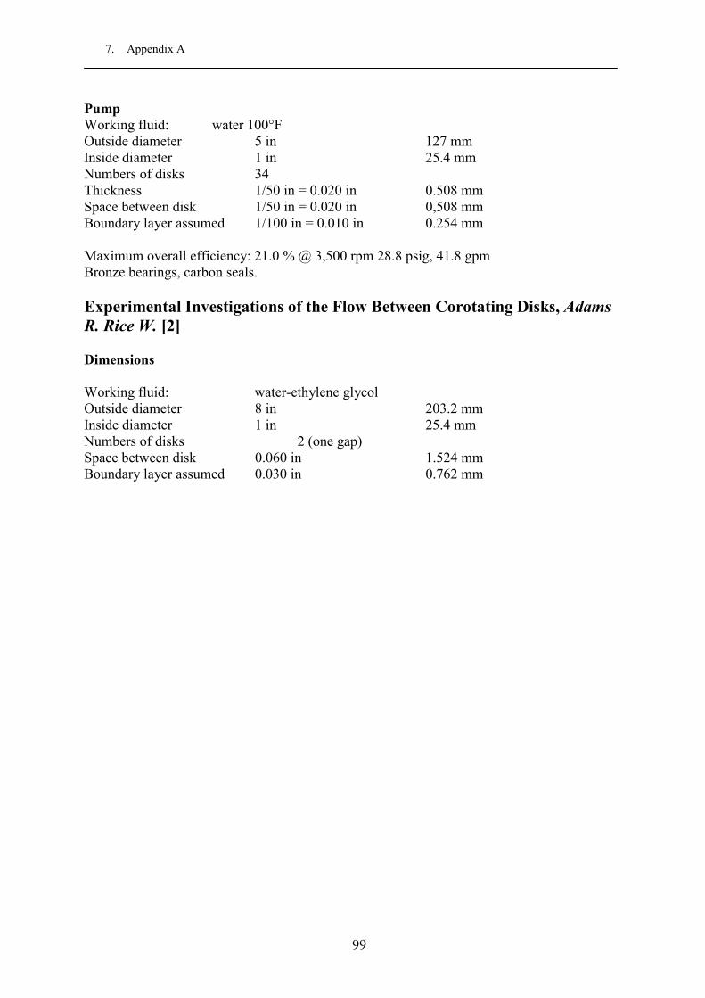
7. Appendix A
Pump Working fluid: water 100°F Outside diameter 5 in 127 mm Inside diameter 1 in 25.4 mm Numbers of disks 34 Thickness 1/50 in = 0.020 in 0.508 mm Space between disk 1/50 in = 0.020 in 0,508 mm Boundary layer assumed 1/100 in = 0.010 in 0.254 mm Maximum overall efficiency: 21.0 % @ 3,500 rpm 28.8 psig, 41.8 gpm Bronze bearings, carbon seals. Experimental Investigations of the Flow Between Corotating Disks, Adams R. Rice W. [2] Dimensions Working fluid: water-ethylene glycol Outside diameter 8 in 203.2 mm Inside diameter 1 in 25.4 mm Numbers of disks 2 (one gap) Space between disk 0.060 in 1.524 mm Boundary layer assumed 0.030 in 0.762 mm
[Contents]
99

Appendix B Variation of Reynolds Number in the Flow Between two Disks The purpose of this section is to provide more information of the behaviour of the turbine, specially the variation of a constant parameter (Reb number) was not consider in the investigation; a simple modification of the values for the simulation of Adams presented in (section 5.10) for the Reynolds number, was made in order to see what happens with the efficiency, when this number is changed. The change of the Reynolds number can be understood from different points of view, change of the velocity of operation, change of the geometry, and finally change of the working fluid. In the model the variable changed was the viscosity. For this simulation the same geometry of Adams and Rice [2], and model were retained. In general, the same settings of simulation in section (5.10). The solution was made for turbulent case and the results agree with those obtain by Lawn and Rice [22], which stated that maximum efficiencies values where found for a value of Reb = 4. The work of Lawn and Rice presents results for idealized turbines as having no losses external to the rotor. Settings: Number Reynolds Reb= 4.291 Radial Velocity Uo
*= -0.2338 [-] Tangential Velocity Vo
*= 0.7793 [-] Angle of the nozzle � = 16.7° Viscosity in non-dimensional with [-]. 0013655.0*
�v 1*��
Mass flow rate [-] 5.334*�m�
Angular speed [-] 005859.0*��
Reynolds number Reb=�b2��
0 5 10 15 20
Efficiency�������
0
5
10
15
20
25
30
Re vs Efficiency
�
�
Totalo
shaf
pm
tP
��
�
Figure B.1.: Efficiency vs. Reynolds number.
The Figure B.1 shows the changes of efficiency for different Reynolds numbers (Reb), with a peak in a value near Reb = 4. Reynolds numbers higher than 20 do not present significant variation. [Contents]
100
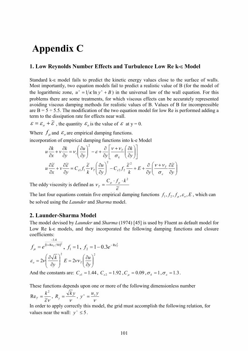
Appendix C
1. Low Reynolds Number Effects and Turbulence Low Re k-� Model Standard k-� model fails to predict the kinetic energy values close to the surface of walls. Most importantly, two equation models fail to predict a realistic value of B (for the model of the logarithmic zone, By ��
�� ln1 �u ) in the universal law of the wall equation. For this problems there are some treatments, for which viscous effects can be accurately represented avoiding viscous damping methods for realistic values of B. Values of B for incompressible are B = 5 ÷ 5.5. The modification of the two equation model for low Re is performed adding a term to the dissipation rate for effects near wall.
���~
�� o , the quantity � is the value of at y = 0. o �
Where and � are empirical damping functions. �f o
incorporation of empirical damping functions into k-e Model
��
���
����
�
�
�
����
�
�
�
�
�
yk
yyu
ykv
xku
k
Tt
�
��
��
2
���
����
�
�
��
�
�����
�
����
�
�
�
�
��
�
�
yyE
kfC
yu
kfC
yv
xu T
T�
�
���
�
���
�
��
~~~~~ 2
22
2
11
The eddy viscosity is defined as �
��
~2kfC
T
��
��
The last four equations contain five empirical damping functions , which can be solved using the Launder and Sharma model.
Efff o ,,,, 21 ��
2. Launder-Sharma Model The model devised by Launder and Sharma (1974) [45] is used by Fluent as default model for Low Re k-� models, and they incorporated the following damping functions and closure coefficients:
� �250Re14.3
Tef �
�
�� , , 11 �f
2Re2 3.01 Tef �
��
2
2 ���
����
�
�
��
yk
o ��
2
2 ���
����
�
�
��
yuE T��
And the constants are: , , ,� ,� . 44.11 ��C 92.12 �
�C 09.0�
�C 1 .1�
��k 3
These functions depends upon one or more of the following dimensionless number
��~Re
2kT � ,
�
ykRy � , �
�yu
y ��
In order to apply correctly this model, the grid must accomplish the following relation, for values near the wall: . 5�
�y[Contents]
101

8. 10. BIBLIOGRAPHY
Bibliography Literature about Turbines
1. Elkouh A.F., Sollenberger C.L., McFarlin D.: A Gas-Turbine for High Temperatures, Research Division Allis-Chalmers Manufacturing Company. Dec., 1961.
2. Adams, R., Rice, W.: “Experimental Investigation of the Flow Between Corotating Disks”, Journal of Applied Mechanics, Vol. 37, Trans. ASME, Vol. 92 series E, No. 3, September 1970, pp. 844-849.
3. Bertin, J. J.: “Mecánica de Fluidos para Ingenieros”, Prentice-Hall S.A., Mexico, 1986
4. “Bladeless Turbines,” Engineering, 92: 637 (1911)
5. Boyack, B.E., Rice, W.: “Integral Method for Flow Between Corotating Disks”, Journal of Basic Engineering, Trans. ASME, Vol. 93 series D, No. 3, September 1971, pp. 350-354.
6. Boyd, K.E., Rice, W.: “Laminar Inward of an Incompressible Fluid Between Rotating Disks, With Full Peripheral Admission”, Journal of Applied Mechanics, Vol. 35, No. 2, Trans. ASME, Vol. 90 series E, June 1968, pp. 229-237.
7. Buckingham, E. "Model Experiments and the Form of Empirical Equations." Trans. ASME 37, 263, 1915.
8. Denton, J.H.: “Loss Mechanism in Turbomachines”. ASME Journal of Turbomachinery, Vol. 115, 621-656, October, 1993.
9. DISKFLO - Manufacturer of Pumps. 10850 Hartley Rd, Santee, CA 92071 [online] Available in internet: <URL:http://www.diskflo.com>.
10. Doyle, Sean.: “AOL CD Tesla Turbine Project”, [online] Available in internet: <URL:http://www.phoenixnavigation.com/ptbc/articles/ptbc30.htm.>
11. Euteneuer G.-A., Piesche, M.: „Betriebsverhalten einer Reibungsturbine bei Turbulentem Stromfeld und Viskosem, Inkompressiblem Medium im Spaltelement”, Forsch. Ing.-Wes. 44 1978, s. 79-84.
12. Experimental Test and Turbine Photos, [online] Available in internet: <URL:http://www.land.salzburg.at/htblha/ingpro99/fuchs/start.html.> April 2002, Graz, Austria.
13. Schultz-Grunow F.: „Der Reibungswiderstand Rotierender Scheiben in Gehäusen”. Kaiser Wilhem Institut fuer Strömungsforschung, Kassel, Juli, 1935.
14. Felsch, K. O., Piesche, M.: „Ein Beitrag zur Berechnung der Strömung in einer Tesla Turbine bei Temperatureabhängiger Zähigkeit des Fördermediums”, Ingenieur-Archiv 50, 1981, Karlsruhe s. 121-129.
15. Felsch, K. O., Piesche, M.: „Zum Betriebsverhalten einer Reibungsturbine und deren Einsatz als Wärmetauscher”, Strömungsmechanik und Stromungsmachinen 27, 1979, s. 1-19.
16. Fluent 6.1. Users manual, © Fluent Incorporated. 2003-01-28.
17. Gambit 2.1.2. Users Manual, © Fluent Inc. 2001-10-29
18. Garrison, P. W., Harvey, D. W., Catton I.: “Laminar Compressible Flow Between Rotating Disks”, Journal of Fluids Engineering, Trans. ASME, Vol. 98 No. 3, September 1976, pp. 382-389.
102

8. 10. BIBLIOGRAPHY
19. Haroutunian, V. Engelman, M.S.: “On Modeling Wall-bound Turbulent Flows using specialized Near-Wall Finite Elements and the Standard k-� Turbulence Model. First ASME/JSME Conference, Fed-Vol. 117, 97-105, 1991.
20. Lakshminarayana B.: Fluid Dynamics and Heat Transfers of Turbomachinery, John Wiley and Sons Inc, New York. 1996, ISBN 0-471-85546-4.
21. Launder, B.E., Spalding, D.B.: “The Numerical Computation of Turbulent Flows”, Computer Methods Appl. Mech. Eng., 3, pp. 269-289, 1974.
22. Lawn, Jr. J., Rice, Warren.: “Calculated Design Data for the Multiple Disk Turbine using Incompressible fluid”, Journal of Fluids Engineering, Trans. ASME, Vol. 96 No. 3, September 1974, pp. 252-258.
23. Logan E., Jr.: “Handbook of Turbomachinery”, Marcel Dekker Editor, Arizona State University, Tempe, Arizona, 1994, pp. 57-69.
24. Matsch, L., Rice, W.: “An Asymptotic Solution for Laminar Flow of an Incompressible Fluid Between Corotating Disks”, Journal of Applied Mechanics, Vol. 35, Trans. ASME, Vol. 90 series E, March 1968, pp. 155-159.
25. Mayle, R. E.: “The Role of Laminar-Turbulent Transition in Gas Turbine Engines”, Transaction of the ASME 91-GT-261, Troy, New York, June 1991.
26. Nendl, D.: „Dreidimensionale Laminare Instabilitäten bei Ebenen Wänden”, Zamm 56, 1976, s. 211-213.
27. Nendl, D.: „Reibungsturbine”, VDI –Berichte Nr. 193 1973, s. 287-293.
28. Nendl, D.: „Eine theoretische Betrachtung der Reibunsturbomaschinen von Nikola Tesla“. Doktor-Ingenieurs Dissertation. Lehrstuhl fuer Technische Mechanik, Technische Hochschule Aachen, July 1966.
29. O'Neill, John J. "Prodigal Genius: Biography of Nikola Tesla, USA, New York, July 15, 1944.
30. Piesche, M.: „Berechnung der Kompressiblen, Laminaren Unterschallströmung in einer Tesla Turbine”, Strömungsmechanik und Stromungsmachinen 28, 1980, s. 25-31.
31. Rhetta, J.: “The Tesla Bladeless Pumps and Turbines”, Proceedings of the Intersociety Energy Conversion Engineering Conference, Vol. 4. IEEE Piscataway, NJ, USA,1991.
32. Rice, W.: “An Analytical and Experimental Investigation of Multiple-Disk Turbines”, Journal of Engineering for Power, Trans. ASME, series A, Vol. 87, No. 1 Jan. 1965, pp. 29-36.
33. Schetz A.J., Fuhs, a.e.: “Fundamental of Fluid Mechanics”, John Wiley and Sons Inc, New York. 1999, ISBN 0-471-34856-2.
34. Schmidt, Darren D.: “Biomass Boundary Layer Turbine Power System”, California Energy Commission (CEC), EISG PROGRAM [online] Available from Internet: <URL: http://eisg.sdsu.edu/Fullsums/00-06.htm > <URL: http://eisg.sdsu.edu/shortsums/shortsum0006.htm>, 1991, California, USA. <URL: http://eisg.sdsu.edu/Far/00-06%20FAR.pdf>
35. Staged Bladeless Turbine Automobile, Partnership for a New Generation of Vehicles, PNGV, Program US. [online] Available in internet: <URL:http://www.geocities.com/vair65_2000>
36. Tabatabai, M.: “On the Process of Inverse Transition in Radial Flow Between Parallel Disks”, H. W. Liepmann, R. Narasimha, Turbulence Management and Relaminarisation, Springer Verlag, Proceedings of the IUTAM Symposium Banglore, India, 1987.
37. Tesla, N.: “Turbine” United States Patent No. 1061206, May 6, 1913.
38. “Tesla´s New Method of and Apparatus for Fluid Propulsion,” Electrical Rev., Sept. 9: 515-517 (1911)
103

8. 10. BIBLIOGRAPHY
39. “The Tesla Steam Turbine,” Eng. News, 66: 448-449 (1911)
40. “The Tesla Steam Turbine,” Sci. Am., Sept. 30: 296-297 (1911)
41. “The Tesla Turbine,” Electrical Rev., Sept. 30: 673 (1911).
42. Truman C. R., Rice W., Jankowski, D. F.: “Laminar Throughflow of Varying-Quality Steam Between Corotating Disks”, Journal of Fluids Engineering, Trans. ASME, Vol. 100, No. 2, June 1978, pp. 194-200.
43. Truman C. R., Rice W., Jankowski, D. F.: “Laminar Throughflow of a Fluid Containing Particles Between Corotating Disks”, Journal of Fluids Engineering, Trans. ASME, Vol. 101, No. 2, March 1979, pp. 87-92.
44. Unix, Eine Einführung in die Benutzung, März 1998, Hannover Universitaet.
45. Wilcox, D.C.: “Turbulence Modeling for CFD” DCW Industries, Inc. La Cañada, California, 1993.
46. Willinger, R.: Vorlesungen über Rechnergestützte Auslegung der Thermischer Turbomaschinen und thermischer Energieanlagen. Vorlesung-skriptum. TU-Wien 2003 - 2004.
[Contents]
Literature about Tesla Pumps
Additional reference literature about source flow for flow between corotating disks, (Pumps, fans, compressors).
47. Bakke, E., Kreider, J. F., Kreith, F.: “Turbulent Source Flow Between Parallel Stationary and Co-rotating Disks”, Journal of Fluids Mechanics, Vol. 58, Part 2, 1973, Great Britain pp. 209-231.
48. Bakke, E., Kreith, F.: “Disk Pump Performance in Turbulent Flow”, ASME Paper 77 WA/FE, 1977.
49. Barske, U. M.: “Development of some Unconventional Centrifugal Pumps”, Proc. Instn Mech Engrs, Vol. 174. No. 11, 1960.
50. Breiter, M. C. , and Pollhausen, K., “Laminar Inward Flow Between Two Parallel Rotating Disks”, Report No. ARL 62-218, Aeronautical Research Laboratories, Wright-Patterson Air Force Base, Dayton, Ohio, March 1962
51. BYALÝl et al B. N.: “Design Characteristics of Multiple-disk Friction Pumps”, Russian Engineering Journal, Vol. LI, No. 9, 1971, pp. 56-60.
52. Cabiev, O. N.: „Zur Berechnung der Kennlinie einer Vielscheibenpumpe bei Förderung Viskoser Flüssigkeiten” Wissenschaftlice Zeitschrifft der Technischen Universitaet Dresden No. 24, 1975, s. 1401-1403.
53. Crawford M. E., Rice W.: “Calculated Design Data for the Multiple-Disk Pump Using Incompressible Fluid”, Journal of Engineering for Power, Trans. ASME, Vol. 96, No. 2, July 1974, pp. 274-281.
54. Felsch, K. O., Piesche, M.: „Das Betriebsverhalten von Reibungsturbomaschinen”, VDI-Berichte Nr. 424, 1981, Karlsruhe s. 265-271.
55. Hasinger S. H., Kehrt, L.G.: “Investigation of a Shear-Force Pump”, Journal of Engineering for Power, Trans. ASME, Vol. 85, Series A No. 3, July 1963, pp. 201-207.
56. Köhler, M.: „Die Strömung durch das Spaltelement einer Reibungspumpe”, Strömungsmechanik und Strömungsmaschinen, Nr 9, February 1971, Karlsruhe s. 24-45.
104

8. 10. BIBLIOGRAPHY
57. Köhler, M.: „Die Strömung Zwischen Zwei Parallelen, Rotierenden Scheiben”, Acta Mechanica 12, 1971, Karlsruhe s. 33-51.
58. Kreith F.: “Reverse Transition in Radial Source Flow between Two Parallel Planes”, The Physics of fluids, Vol. 8, No. 6, June 1965, pp. 1189-1190.
59. Miller, G.E., Sidhu, A., Fink, R. and Etter, B.D., “Evaluation of a Multiple Disk Pump as an Artificial Ventricle, Artificial Organs, 17: 590-592, 1993.
60. Mochizuki, S., Inoue, T.: “Self-Sustained Flow Oscillations and Heat Transfer in Radial Flow Through Co-Rotating Parallel Disks”, Experimental Thermal and Fluid Science, Nr. 3, 1990 pp. 242-248.
61. Mochizuki, S., Tanida, Y.: “Unsteady Flow Phenomena in Multiple Disk Fans”, ASME Paper 79 FE-10, 1979.
62. Murata, S., Miyake, Y,. Iemoto, Y.: “A Study on a Disk Friction Pump”, Bulletin of J.S.M.E. Vol. 19, No. 128, February 1976, pp. 168-178.
63. Murata, S., Miyake, Y,. Iemoto, Y.: “A Study on a Disk Friction Pump, 2nd report, Experiments on Flow through Corotating Disks and Pump Performance”, Bulletin of J.S.M.E. Vol. 19, No. 136, October 1976, pp. 1160-1171.
64. Nendl, D.: „Eine Theoretische Betractung der Tesla-Reibungspumpe”, VDI-Forsh.Heft 527, 1973, Aachen, s . 29-36.
65. Osterwalder, J.: „Experimentelle Untersuchungen mit einer Reibungspumpe”, Konstruktion No. 35, 1983, Darmstadt, s. 187-190.
66. Pater, L. L., Crowther E., Rice, W.: “Flow Regime Definitions for Flow Between Corotating Disks”, Journal of Fluids Engineering, Trans. ASME, Vol. 96, March 1974, pp. 29-34.
67. Piesche, M., Felsch, K. O.: „Berechnung der Spaltströmung in einer Reibungspumpe bei Temperaturabhängiger Viskosität” Acta Mechanica No. 38, 1981, Karlsruhe, s. 99-107.
68. Piesche, M., Felsch, K. O.: „Kompressible Unterschallströmungen in Reibungsverdichtern” Acta Mechanica No. 41, 1981, Karlsruhe, s. 99-107.
69. Piesche, M., Müller U.: „Über den Wärmetransport im Spaltelement einer Reibungspumpe” Acta Mechanica No. 35, 1980, s. 175-186.
70. Piesche, M.: „Betriebseigenschaften konventioneller Laufradgitter radialer Bauart im Vergleich mit Spaltelementen von Reibungspumpen”, Strömungsmechanik und Strömungsmachinen No. 31, 1982, s. 1-21.
71. Rice, W.: “An Analytical and Experimental Investigation of Multiple-Disk Pumps and Compressors”, Journal of Engineering for Power, Trans. ASME, series A, Vol. 85, No. 3 July, 1963, pp. 191-198.
72. S. A. Shirazi, C. R. Truman.: “Prediction of turbulent Source Flow Between Corotating Disks with an Anisotropic Two-Equation Turbulence Model“, ASME Paper 87-G-73 1987, California.
[Contents]
105

List of Figures Figure 2.1. American patent No. 1,061,206 of Tesla turbine [37]. .............................................. 3 Figure 2.2 Power-speed characteristics of an air turbine at selected input pressures [32]. ...... 4 Figure 2.3. Efficiency-speed characteristics of an air turbine at selected input pressures [32].. 4 Figure 2.4.: Typical results for maximun efficiency as a funtion of flow rate and speed parameter. Plotted for f=0.05, ro/b=50 [32]. ............................................................................... 5 Figure 2.5.: Typical results for pressure-change parameter as a function of flow rate and speed parameters. Plotted for f= 0.05, ro/b=50 [32].................................................................... 5 Figure 2.6.: Constant efficiency lines on Re and Uo*, for Vo*= 1.1, r* = 0.3, and parabolic inlet velocities [22]........................................................................................................................ 7 Figure 2.7. Tangential velocity profile through gap with different Reb numbers [27]. ................ 8 Figure 2.8. Principle of energy transfer through friction. ............................................................ 9 Figure 3.1. Schematic diagram of Tesla turbine [23]................................................................. 11 Figure 3.2. Geometry of an isolated rotor, section A-A´. ........................................................... 11 Figure 3.3. Runner of 26 disks [12]. ........................................................................................... 12 Figure 3.4. A single flat disk with star spacers washers and rivets [35].................................... 12 Figure 3.5. Triangle of velocities for the Tesla turbine. ............................................................. 13 Figure 3.6. Schematic diagram of the turbine showing the path of fluid [32]............................ 13 Figure 3.7.: Detail of the velocity inlet and coordinates. ........................................................... 14 Figure 3.8.: Diagram h-s for the rotor and stator. ..................................................................... 14 Figure 3.9.: Laminarization and transition modes present in the gap. ...................................... 16 Figure 3.10.: Losses in disk turbine. ........................................................................................... 17 Figure 4.1. Control volume approach......................................................................................... 22 Figure 4.2.: Difference of the stagnation pressure for compressible or incompressible flow.... 28 Figure 4.3.: Behaviour of the degree of reaction vs. flow rate with constant inlet angle as a parameter .................................................................................................................................... 30 Figure 4.4.: Behaviour of the degree of reaction vs. inlet angle with the flow rate as a parameter. ................................................................................................................................... 31 Figure 4.5.: Fluid Sheared between two plates [33]. ................................................................. 32 Figure 4.6.: Linear or nonlinear stress/strein rate behaviour [33]............................................ 32 Figure 4.7.: Typical Radial Distribution of tangential velocity in a free vortex [16]. ............... 33 Figure 4.8.: Velocity fluctuation for turbulence Model. ............................................................. 34 Figure 4.9.: Bursting process in transition from laminar to turbulent [33]............................... 36 Figure 4.10.: The flat plate Boundary layer (a) geometry with the boundary layer thickness and (b) typical shear and heat flux distributions [33]. ............................................................... 37 Figure 4.11.: Natural transition to turbulent over a flat plate [33]. .......................................... 37 Figure 4.12.: Schematic representation of laminar and turbulent boundary layer. ................... 39 Figure 4.13.: Plot of the boundary layer of the solution of Blausius for a flow over a flat plate. ............................................................................................................................................ 40 Figure 5.1.: Geometry for CFD model, one gap model. ............................................................. 43 Figure 5.2.: Mesh for the entire rotor. ........................................................................................ 44 Figure 5.3.: Detail of the mesh of Figure 5.2. ............................................................................ 45 Figure 5.4.: 2D mesh for laminar and turbulent model with full resolution at the wall. ........... 45 Figure 5.5.: Mesh at the middle radius. ...................................................................................... 46 Figure 5.6.: Mesh for using wall functions in k-� turbulence model. ......................................... 47 Figure 5.7.: Convergence of laminar solution............................................................................ 49 Figure 5.8.: Controling the convergence of swirl velocity at the outlet. .................................... 49 Figure 5.9.: Velocity magnitude laminar solution, non-dimensional values. ............................. 50
106

LIST OF FIGURES AND TABLES
Figure 5.10.: Radial velocity, laminar solution, non-dimensional values. ................................. 51 Figure 5.11.: Inflection of radial velocity for different radial stations, dimensional values...... 51 Figure 5.12.: 3D plot of the velocity magnitude at the outlet of the rotor, dimensional values. 52 Figure 5.13.: Tangential velocity plotted with velocity magnitude............................................. 52 Figure 5.14.: Axial velocity laminar solution, non-dimensional values. .................................... 53 Figure 5.15.: Total, dynamic and static pressure distribution along radius, laminar solution..53 Figure 5.16.: Total pressure for different radial station, laminar solution. .............................. 54 Figure 5.17.: Variation of tangential wall shear stress along the radius, laminar and non-dimensional values. ..................................................................................................................... 54 Figure 5.18.: Contours of stream functions at three radial stations........................................... 55 Figure 5.19.: Contours of axial velocity at inlet and outlet. ....................................................... 55 Figure 5.20.: Characteristic curve, loading coefficient., laminar solution. ............................... 56 Figure 5.21.: Characteristic curve, dimensional values. ........................................................... 56 Figure 5.22.: Efficiency of an isolated disk, laminar solution.................................................... 57 Figure 5.23.: Degree of reaction for the laminar solution. ........................................................ 57 Figure 5.24.: Geometry for the Adams experiment simulation................................................... 59 Figure 5.25.: Comparison numerical solutions with experiment from Adams and Rice [2]...... 60 Figure 5.26.: Values of y+ for the cells adjacent to the walls. ................................................... 62 Figure 5.27.: Velocity magnitude, turbulent case. ...................................................................... 62 Figure 5.28.: Radial velocity, turbulent case.............................................................................. 63 Figure 5.29.: Tangential velocity, turbulent case. ...................................................................... 63 Figure 5.30.: Axial velocity, turbulent case. ............................................................................... 64 Figure 5.31.: Plot of vectors in 2D plane. .................................................................................. 64 Figure 5.32.: Velocity magnitude through radius, V*= 1.1, U*= -0.4. ....................................... 65 Figure 5.33.: Plot of local Reynolds number along the radius, turbulent case. ........................ 66 Figure 5.34.: Total, dynamic and static pressure curve along the radius, turbulent case. ........ 66 Figure 5.35.: Flow angles values along the radius, turbulent case............................................ 67 Figure 5.36.: Loading coefficient for turbulent solution, isolated disk. ..................................... 67 Figure 5.37.: Efficiency for turbulent solution, isolated disk. .................................................... 68 Figure 5.38.: Degree of reaction for turbulent solution in comparison with laminar solution, isolated disk................................................................................................................................. 68 Figure 5.39.: Contours of pressure at the outlet of the gap........................................................ 69 Figure 5.40.: Dynamic pressure through the radius................................................................... 70 Figure 5.41.: Static pressure through the radius. ....................................................................... 70 Figure 5.42.: Total pressure through the radius......................................................................... 71 Figure 5.43.: Distribution of the acceleration parameter for the radial flow between disks. .... 71 Figure 5.44. 2D model of the turbine with full peripheral admission. ....................................... 72 Figure 5.45.: Convergence of 2D turbine model. ....................................................................... 73 Figure 5.46.: Convergence history of static presssure for 2D turbine model. ........................... 73 Figure 5.47.: Loading coefficient for turbulent solution, turbine. .............................................. 74 Figure 5.48.: Efficiency for turbulent solution, turbine. ............................................................. 74 Figure 5.49.: Degree of reaction for turbulent solution, turbine............................................... 75 Figure 5.50.: Detail of the grid. .................................................................................................. 76 Figure 5.51.: Values for y+ along the housing wall. ................................................................... 76 Figure 5.52.: Plot of vector of velocities at the trailing edge. ................................................... 77 Figure 5.53.: Plot of vector of velocities at the leading edge. ................................................... 77 Figure 5.54.: Plot of vector of velocities at the leading edge, detail at last disk....................... 78 Figure 5.55.: Plot of vector of velocities at the outlet of the rotor. ........................................... 78 Figure 5.56.: Plot of vector of velocities at the center of the turbine. ....................................... 79 Figure 5.57.: Path lines along the turbine. ................................................................................. 79
107

LIST OF FIGURES AND TABLES
Figure 5.58:. Detail of path lines at the leading edge, the plot shows the half of the rotor. ...... 80 Figure 5.59.: Detail of path lines at the leading edge between two disks. ................................. 80 Figure 5.60.: Detail of path lines at the trailing edge. ............................................................... 81 Figure 5.61.: Contours of pressure for the Tesla turbine. .......................................................... 81 Figure 5.62.: Details of contours of pressure for the Tesla turbine at the outle of the rotor. .... 82 Figure 5.63.: Side view of one slide for the tesla turbine. .......................................................... 82 Figure 5.64.: 3D plot of the domain with subdivisions in smaller volumes................................ 83 Figure 5.65.: Mesh for the 3D slide model. ................................................................................ 84 Figure 5.66.: Detail of the mesh at the nozzle ............................................................................ 84 Figure 5.67.: Detail of the mesh at the outlet. ............................................................................ 85 Figure 5.68.: Detail of the mesh of the disk. ............................................................................... 85 Figure 5.69.: Convergence history of residuals.......................................................................... 87 Figure 5.70.: Convergence history of velocity magnitude. ......................................................... 88 Figure 5.71.: Loading coefficient for 3D slide model................................................................. 88 Figure 5.72.: Efficiency of 3D slide model ................................................................................. 90 Figure 5.73.: Path lines colored by velocity magnitude. ............................................................ 90 Figure 5.74.: Contours of total pressure at the surface of the disks........................................... 90 Figure 5.75.: Contours of total pressure at the middle of the gap.............................................. 90 Figure 5.76.: Contours of total pressure at leading edge in the middle of the rotor.................. 91 Figure 5.77.: Vectors of velocity magnitude and total pressure contours at the middle of the gap............................................................................................................................................... 91 Figure 5.78.: Detail of vectors of velocity magnitude near the wall of the housing................... 92 Figure 5.79.: Veloctiy magnitude, through the radius. ............................................................... 92 Figure 5.80.: Contours of axial velocity at the middle of the gap. ............................................. 93 Figure 5.81.: Wall shear stress over the disk.............................................................................. 93 Figure B.1.: Efficiency vs. Reynolds number. ........................................................................... 100
[Contents]
List of Tables Table 2.1. Non-dimensional parameters and characteristics of tested turbines........................... 7 Table 3.1.: Materials pumped by the bladeless pumps [31] . ..................................................... 19 Table 3.2.: Performance of boundary layer turbine tested and reported by Schmidt [34]. ...... 21 Table 4.1.: Summarize of principal parameters that describe the Tesla turbine........................ 31 Table 4.2.: Constants of k-� model.............................................................................................. 36 Table 5.1.: General parameters used in Fluent. ......................................................................... 42 Table 5.2.: Geometry of domain.................................................................................................. 42 Table 5.3.: Values for meshing the edges, 2D model. ................................................................. 44 Table 5.4.: Relaxation factors. .................................................................................................... 47 Table 5.5.: Properties of working fluid. ...................................................................................... 47 Table 5.6.: Data for laminar simulation. .................................................................................... 48 Table 5.7.: Summarize of performance of the turbine for laminar solution. .............................. 58 Table 5.8.: Turbulent boundary conditions at the inlet............................................................... 61 Table 5.9:. Summarize of performance of the turbine for turbulent solution. ........................... 69 Table 5.10.. Summarize of performance of the turbine for turbulence solution. ........................ 75 Table 5.11.: Values for meshing the edges, 3D model. ............................................................... 86 Table 5.12.: Velocity inlet values for the nozzle. ........................................................................ 87
[Contents]
108