numerical simulation of the flow through an axial …
TRANSCRIPT

FERNANDO MATTAVO DE ALMEIDA
NUMERICAL SIMULATION OF THE FLOW
THROUGH AN AXIAL TIDAL-CURRENT TURBINE
EMPLOYING AN ELASTIC-FREE-SURFACE
APPROACH
Dissertation presented to the Escola
Politécnica of the University of São
Paulo for the degree of Master of
Science in Engineering
São Paulo
2018

FERNANDO MATTAVO DE ALMEIDA
NUMERICAL SIMULATION OF THE FLOW
THROUGH AN AXIAL TIDAL-CURRENT TURBINE
EMPLOYING AN ELASTIC-FREE-SURFACE
APPROACH
Dissertation presented to the Escola
Politécnica of the University of São
Paulo for the degree of Master of
Science in Engineering.
Concentration Area:
Naval Architecture and Oceanic Engineering
Advisor:
Prof. Dr. Gustavo Roque da Silva Assi
São Paulo
2018

Catalogação-na-publicação
Mattavo, Fernando
Numerical Simulation of the Flow Through an Axial Tidal-Current Turbine Employing an Elastic-Free Surface Approach / F. Mattavo -- versão corr. -- São Paulo, 2018.
152 p.
Dissertação (Mestrado) - Escola Politécnica da Universidade de São Paulo. Departamento de Engenharia Naval e Oceânica.
1. MECÂNICA DOS FLUÍDOS COMPUTACIONAL, FONTES RENOVÁVEIS DE ENERGIA, ENERGIA MARÉMOTRIZ, TURBINAS HIDRÁULICAS I.Universidade de São Paulo. Escola Politécnica. Departamento de Engenharia Naval e Oceânica II.t.

Nome: MATTAVO, Fernando
Título: Numerical Simulation of the Flow Through an Axial Tidal-Current
Turbine Employing an Elastic-Free Surface Approach
Dissertação apresentada à Escola Politécnica da
Universidade de São Paulo para a obtenção do título
de Mestre em Engenharia
Aprovado em: 15/06/2018
Banca Examinadora
Prof. Dr. Gustavo Roque da Silva Assi
Instituição Escola Politécnica da Universidade de São Paulo
Julgamento Aprovado
Prof. Dr. Fábio Saltara
Instituição Escola Politécnica da Universidade de São Paulo
Julgamento Aprovado
Prof. Dr. Reinaldo Marcondes Orselli
Instituição Universidade Federal do ABC
Julgamento Aprovado

Dedicatory
First of all, I dedicate this work for my mother, Maria de Lourdes, who fulfilled
me with love and gave all the support I have needed in my whole personal,
professional and academic life, fulfilling me with courage and enthusiasm to
face the most difficult challenges.
I also remember my colleagues and professors from Universidade de São
Paulo, who made possible the conclusion of this work and are fundamental
parts of my academic journey. Specially, I would like to dedicate this work for
my advisor PhD Gustavo Assi, who helped me in critical moments of this work
and gave me fundamental insights for the continuity of the development of my
Master Degree. I would like to dedicate also this work for the Professor Celso
Pesce, being fundamental for the development of my critical sense and
analytical personality, inspiring me for being an open minded person who
always looks for knowledge.
I would like to dedicate this work to my colleagues from Voith Hydro Ltda., who
gave me support in my professional career, contributing to my personal
evolution since April of 2013. I have a special dedicatory for Ph.D. Humberto
Gissoni, who gave me the opportunity and the incentives always to keep
developing myself, for Leonardo Silva, who supported me and in difficult
moments of my life, showed interest in helping, being a valuable friend, for MSc.
Leandro Bernardes, who always supported me and inspired me for the scientific
development and for all other colleagues that helped me in my professional
career.
Finally, I dedicate this work for all of my Friends, who always believed me and
were fundamental parts from my life, even in the difficult moments, when they
were at my side to guide me through the most challenging paths from my
personal and professional life.

“I am just a child who has never grown up. I still keep asking these ‘how’ and ‘why’ questions. Occasionally, I find an answer”.
(Stephen Hawking)

Resumo
O crescimento econômico mundial e o aumento na demanda pela geração de
energia andam juntos. No entanto, uma maior capacidade de produção de
energia poderia afetar negativamente o meio ambiente. Mesmo as fontes
limpas e renováveis, como a hidrelétrica e a eólica acarretam em impactos
socioeconômicos e ambientais. Por exemplo, a construção de uma usina
hidrelétrica demanda uma imensa área alagada que pode devastar florestas
inteiras e a instalação de uma usina eólica pode afetar a migração de certas
espécies de pássaros e produzir altos níveis de barulho.
Portanto, para equilibrar as vantagens e desvantagens devidas a cada meio de
produção de energia, é necessária a diversificação, que demanda de
investimentos em novas fontes. Neste contexto, a geração de energia nos
oceanos é destacada. O primeiro ponto a respeito desta fonte é de que não há
a necessidade de remoção da população na área de instalação, tal como os
métodos de geração dentro do continente. O segundo principal ponto é a
respeito da distribuição de energia. A maior parte da população mundial vive
em regiões costeiras, diminuindo, portanto, a distância entre a produção e
demanda, reduzindo assim, seus custos.
As duas principais metodologias para se explorar a energia proveniente dos
oceanos são: Energia de Ondas e Energia de Marés. E considerando que os
ciclos de mare são governados principalmente pela interação gravitacional
entre os oceanos, lua e sol, eles são facilmente previsíveis, o que aumenta a
confiabilidade dos sistemas de geração de energia baseados em marés.
Este trabalho explora as metodologias para analisar a geração de energia a
partir de uma única turbina axial de corrente de maré através de uma
metodologia baseada nas equações de Navier-Stokes com a média de
Reynolds, analisadas em regime permanente. São discutidos efeitos da direção
do escoamento, perfil de velocidades na entrada e nos níveis de turbulência.
Os resultados são comparados com experimentos.
É proposta uma metodologia alternativa para a modelagem da superfície livre
com CFD uma vez que a metodologia atual é baseada em um escoamento

bifásico que demanda de um refinamento adicional da malha e é
computacionalmente caro. A nova metodologia usa uma parede elástica na
região da superfície livre com a rigidez ajustada para se obter o mesmo efeito
de restauração que a gravidade.
De maneira geral, os resultados para o domínio aberto se aproximaram dos
resultados experimentais, validando o modelo numérico e além disso, o modelo
considerando confinamento da turbine mostrou maiores valores para os
coeficientes de potência e empuxo, estando portanto, de acordo com a teoria
do disco atuador.
O modelo com a superfície livre elástica apresentou problemas de
convergência, relacionados com números de Froude elevados, uma vez que
isto se relaciona com maiores deformações na região da superfície livre. Uma
simulação com 10% da velocidade original foi realizada, obtendo-se resultados
coerentes para ambos coeficientes de potência e empuxo.
Palavras-Chave: Energia do Oceano, Turbinas de Corrente de Maré, Dinâmica
dos Fluídos Computacional (CFD), Modelagem de Superfície Livre

Abstract
Together with the world economic growth is the increasing of energy generation
demand. However, the upgrade of world power production capability could
affect the environment negatively. Even the clean and renewable sources, such
as hydroelectricity and wind powers have socio-economic and environmental
disadvantages. For example, the required flooded area for a hydro power plant
construction could devastate entire forests, and the installation of a wind farm
power plant could affect migratory rotes of birds and generate high levels of
noise.
Hence, for the balancing of advantages and disadvantages of each power
generation source, it is necessary to diversify, which requires investments in
new power sources. In this context, the energy generation in the ocean is
highlighted. The first point concerning the ocean energy is that there is no need
of population removal from the installation area, such as the onshore based
methods and the second point is that most of the population is concentrated in
coastal areas. Therefore the production occurs near to the demand, decreasing
the costs with energy distribution.
The two main methodologies for harassing energy from oceans are based on
gravity waves and in tides. And since the tidal cycles are governed mainly by
the gravitational interaction between oceans, Moon and Sun, they are easily
predictable, which increases the reliability of such systems.
These works explores methodologies to analyse the power generation from a
single axial tidal current turbine through a Steady State RANS methodology.
Are discussed the effects of flow directionality, inlet velocity profile and
turbulence levels and the results are compared with an experimental scheme.
It is proposed an alternative methodology for free surface modelling in the CFD
analysis. The usual methodology, VOF, it is based on a homogeneous, biphasic
approach which requires an additional mesh refinement and is computationally
expensive. This new methodology introduces an elastic wall approach in the
free surface region in which the stiffness is calculated to provide the same
restoring effect as gravity.

In general, the results for open domain matched with the experimental results,
validating the numerical model and the confined domain has shown a higher
power and thrust coefficients if compared with the open domain, which is in
accordance with the actuator disk theory approach.
The elastic free surface presented convergence problems related to high
Froude numbers and therefore to high deformations. However, a simulation with
10% of the original inlet velocity was performed, achieving reasonable results
for both power and thrust coefficients evaluation.
Key Words: Ocean Energy, Tidal Current Turbines, Computational Fluid
Dynamics (CFD), Free Surface Modelling

Contents
Chapter 1. Introduction ........................................................................................... 1
1.1 Motivation ....................................................................................................... 2
1.2 Objectives ...................................................................................................... 4
1.3 Text Structure ................................................................................................. 5
Chapter 2. World Energy Matrix and Renewable Energy Generation .................... 8
2.1 World Energy Matrix ....................................................................................... 8
2.2 Renewable energy usage ............................................................................. 10
2.3 Oceanic energy extraction ............................................................................ 12
Chapter 3. Literature review on tidal axial turbines .............................................. 15
3.1 Tidal Current Turbines .................................................................................. 15
3.1.1 Experimental Analysis ........................................................................... 15
3.1.2 Computational Fluid Dynamics Analysis ................................................ 20
3.1.3 Analytical models ................................................................................... 28
3.1.4 Tidal farm and wind farm optimization methods..................................... 29
3.2 Open channel models .................................................................................. 30
Chapter 4. Theoretical Fundamentals .................................................................. 32
4.1 Basics equations of Fluid Dynamics ............................................................. 33
4.1.1 Turbulence Models ................................................................................ 38
4.2 Potential Fluid Flow ...................................................................................... 42
4.3 Solid Mechanics for Orthotropic Bodies ....................................................... 44
4.4 Computational Methods ............................................................................... 48
4.4.1 Computational Fluid Dynamics (CFD) ................................................... 48
4.4.2 Finite Element Method ........................................................................... 52
Chapter 5. Methodology ....................................................................................... 56
Chapter 6. Free Surface Modelling ...................................................................... 59

6.1 Elastic Free Surface Model .......................................................................... 60
6.1.1 Orthotropic Solid Transversal Stiffness Calculation ............................... 60
6.2 Consequences in fluid flow due to substitution of buoyancy for elastic free
surface ................................................................................................................... 63
6.2.1 Waves due to a Submerged Cylinder .................................................... 63
6.2.2 Linear Wave Propagation ...................................................................... 67
6.2.3 Actuator Disk Model for an Open Channel ............................................ 73
6.3 Steady State Finite Element Model from Elastic Free Surface ..................... 76
Chapter 7. CFD Simulations ................................................................................ 80
7.1 General Overview......................................................................................... 81
7.1.1 Rotating Domain Mesh .......................................................................... 83
7.1.2 Subdomains and Domain Interfaces ...................................................... 86
7.2 Open Domain ............................................................................................... 88
7.3 Confined Domain ......................................................................................... 89
7.4 Open Channel Model – Elastic Free Surface ............................................... 89
Chapter 8. Results ............................................................................................... 90
8.1 Open Domain ............................................................................................... 90
8.2 Confined Flow .............................................................................................. 97
8.3 Open Channel ............................................................................................ 101
8.3.1 Flow Analysis ....................................................................................... 102
8.3.2 Deformations in the Solid Model .......................................................... 109
8.4 Comparison Between the CFD Models ...................................................... 111
Chapter 9. Conclusion ........................................................................................ 113
Chapter 10. Proposals for complementary works ................................................ 115
10.1 Tidal current turbines .............................................................................. 115
10.2 Free surface analysis .............................................................................. 116
Chapter 11. References ....................................................................................... 118

ATTACHMENT A – Potential Fluid Flow ................................................................. 126
A.1 – Flow through a circular cylinder .................................................................. 126
A.2 – Gravity Waves ............................................................................................ 127
ATTACHMENT B – 𝒌- 𝝎 – SST Model .................................................................... 134
ATTACHMENT C – Wall Functions ......................................................................... 136
ATTACHMENT D – Actuator Disk Theory ............................................................... 138
Open Flow Model (Betz Limit) ....................................................................... 138
Confined Flow Model (Ducted Flow) .............................................................. 141
Single Turbine Placed on Open Channel Flow .............................................. 144
ATTACHMENT E – Tidal Current Turbines ............................................................. 147
Cross Flow Devices ............................................................................................. 147
Axial Devices ....................................................................................................... 148
ATTACHMENT F – Finite Volume Elements ........................................................... 150
Finite Volume Method for Unstructured Meshes............................................ 150

1
Chapter 1. Introduction
All environmental and economic researches point to clean and renewable
energy resources. It is not allowable that in XXI Century to still insist on energy
generation matrix based on thermoelectric power plants. Even the most known
industry for its dependency on fossil fuel, the automotive industry, has
investments in researches to substitute the traditional combustion-based motors
with electric ones, with more autonomy and efficient. The Figure 1 shows the
evolution of the number of the electrical cars stock since 2010. The shape of the
curve reveals its ascendant behavior and the most pessimist prediction points
that in 2030, at least 60 million electric vehicles will be in the street
(International Energy Agency, 2017).
Furthermore, several works highlight the direct dependence between a country
economic growth and its capability of energy generation. In China, was
performed an empirical assessment correlating the economy evolution with the
total energy consumption and its CO2 generation (Wang, Li, Fang, & Zhou,
2016). Considering that several countries are still underdeveloped and even the
developed countries still have its economy growing up, the current world electric
energy production, mainly based on fossil fuel, will contribute raising the CO2
emission, which is already in a worrisome level.
Therefore, is concluded that is expected the growth of the world economy which
leads to an increase in the energy production. Causing impacts on the world
climate and the environment. Based on this, the need for researches and
development in clean energy generation is mandatory for sustainable
development.
For a clean energy generation, there are several methods, most of them
converting the available energy on nature into electrical power, such as wind
power plants that convert the kinetic wind energy and a hydroelectric power
plant that converts the potential gravity energy stored in water reservoirs. Each
energy source with its advantages and problems.

2
Figure 1 - Number of electric cars in the world since 2010
Source: (International Energy Agency, 2017)
A known source of renewable energy it is the ocean. There is available power in
several ways, such as in surface waves, salinity and temperature gradients and
due to tides. An important factor from oceanic energy extraction lies in the early
development stage with prototypes and small power plants that only could
attend a local demand.
Moreover, this work focuses on the extraction of tidal energy, in the form of
kinetic energy due to underwater currents, by placing axial turbines. The main
goal is doing a hydrodynamic performance assessment studying several
factors, such as interaction with the free surface, turbulence, and proximity with
physical boundaries and another neighbor turbine, by a Computational Fluid
Dynamics approach., mainly studying a most computational method for
evaluating free surface effects on turbine performance.
1.1 Motivation
The tidal based energy still need researches focusing on its performance
enhancement, since its generation cost is prohibitive if compared to other
renewable sources (IRENA, 2014). Furthermore, the environmental impacts still
under evaluation since are not completely known the impacts of the turbines
deployment on marine relief, sedimentation, fauna, and flora.
For both issues, a most accurate flow modelling is useful, since it allows
improving the individual turbine efficiency and the whole farm performance and
permits to evaluate the changes in local flow pattern which could affect the

3
seabed relief with impacts on vegetation and in animals that live near to the
installation point.
The complete modelling of flow through a tidal current generation farm includes
full modelling of turbine blades and structure, original velocity profile, and
turbulence levels, channel geometry, free surface effects as its blockage and
the gravity waves, the interaction between the turbines and maritime currents
that could affect flow directionality. Moreover, even for neglecting any effect, is
essential to comprehend its influence in the hydrodynamic performance, such
as power generation, and in other flow parameters such as wake length and
recovery. However, a model including all described flow parameters is
computationally prohibitive, even on supercomputers.
An interesting parameter is the free surface effect on tidal current turbine
hydrodynamic performance and in mechanical loading. Its traditional modelling
uses a biphasic fluid flow with a new flow variable that is the proportion between
the two fluids. To guarantee the convergence, without numerical diffusion
problems and with a reasonable free surface resolution, it is necessary a high
refinement which increases the computational costs.
Besides that, other industrial flows, such as flow around risers, oil platforms,
and other oceanic engineering applications, the free surface effects are not
negligible, and therefore, such problems demand more efficient ways of free
surface modelling.
Hence, the work is focused on flow analysis through an axial tidal current
turbine with special attention in free surface effects, including an artificial Fluid-
Structure Approach to perform a steady-state analysis including free surface
blockage effects. This method is based on energy conservation and applied to
classical fluid mechanics problems such as free surface gravity waves and free
surface deformation due to the potential flow through a circular cylinder
produces the same results from the original theory.

4
1.2 Objectives
Considering the analysis of the flow through an axial tidal current turbine close
to a free surface using Computational Fluid Dynamics. It is necessary to
validate a CFD model with accurate results regarding the experimental ones
and then is necessary to validate and implement a free surface analysis model.
Hence, the first objective of this present work is to define and understand the
flow through the turbine with the simplest domain: The Domain without lateral
boundaries. As seen in the section 4.1.1 there is a set of experimental results
corrected for this domain that could be used as a reference to validate some
CFD parameters such as domain dimensions, turbulence model and mesh
refinement level.
However, both experiment and prototype do not consist of a single turbine
placed on an open domain. There is a confinement level which could increase
the turbine power and wake recovery length. Hence, the confinement effect is
studied in the present work.
For studying such effect, a simulation with slip-free walls in the same
dimensions as the test rig presented in the section 4.1.1 is performed with the
objective of understanding how such confinement affects the flow.
Additionally, tidal current turbines are subjected to free surface effects. The free
surface confines the flow, but less than a slip-free wall, since its deformation
allows a higher portion of fluid deviates the turbine disk. Accordingly, it is
necessary to perform a simulation including such effect. However, it is
necessary to highlight the lack of a computationally efficient methodology for
analyzing such effect. For example, the Volume of Fluid method requires a bi-
phasic simulation including an air domain and an extra refinement in the free
surface region. Then, in the present text, an alternative methodology is
proposed. The new methodology for analyzing free surface is based on energy
conservation and uses an orthotropic solid to have a spring restoring effect in
such region. Therefore, this work focuses on present the theoretical foundation
of such methodology and implements it for the Tidal Current Turbine Analysis.

5
1.3 Text Structure
As discussed in the previous section, this work is focused on the introduction of
an alternative methodology to evaluate the free surface effects in a
Computational Fluid Dynamics simulation applied to an axial tidal current
turbine. Therefore, there is a necessity on reviewing the basics of fluid
dynamics and computational methodology used for solving such kind of
problem. Besides, since there is a new proposed methodology, is necessary to
present the theoretical development which justifies its usage in the presented
problem. And finally, an introduction to the actual scenario and predictions
about world energy generation is necessary so that this research is applied in
an actual and existing matter.
The Chapter 2 provides an overview of the actual status and predictions
regarding the world energy matrix. There is a focus on clean energy,
highlighting the main sources and introducing the oceanic energy sources as an
alternative to green energy production. Justifying the investment necessities in
energy generation is important.
Introduced the potential oceanic energy sources, the actual stage of
development of tidal current turbines is presented, focusing on the
methodologies for extracting tidal current energy. In such context, some
manufacturers and its commercial products are shown in the Chapter 3.
The Chapter 4 presents the most recent works related to the tidal current
turbines. Some experiments are discussed including their methodology and
results which provides the data to validate computational methodologies for
predicting the power and thrust provided by those turbines. The computational
methods that are used for analyzing tidal current turbines are also presented in
this chapter. The section provides a brief analysis discussing the accuracy of
the results according to the analysis goals and the methodology used for
obtaining such results. It is shown a brief introduction in the analytical models,
which are fundamental to understand the main flow physics and the influence of
some boundary conditions in the fluid flow. Besides, even not being the scope
of this work, some articles about tidal current turbine farms optimization are

6
discussed since such analysis could lead to a higher power harvesting using a
lower number of turbines, decreasing the total cost of a tidal current turbine
farm and therefore reducing the energy price. Finally, in this chapter, a
discussion about some current methodologies for evaluating tidal current
turbines is introduced.
For completing this work, is necessary a comprehension about the physics
related to turbulent, viscous and incompressible fluid flow and the main subjects
related to the simulation of such flow in a computational environment. Hence,
the Chapter 5 introduces the basic equations for fluid flow analysis and
introduces the methodologies for analyzing a turbulent flow with accuracy.
Besides, a brief discussion about the finite volume method is performed
highlighting the main features which could influence the results and
computational time of a CFD simulation.
Furthermore, it is included in Chapter 5 the necessary tools for modelling the
free surface as an elastic wall. This methodology is implemented in this text as
an orthotropic solid coupled to the fluid domain. Hence, the basics of solid
mechanics are presented and the necessary hypothesis to guarantee the
necessary behavior for modelling a free surface are discussed. And since that
this solid domain is solved by the Finite Element Method, the basics of such
methodology is presented in the last part of this chapter.
The Chapter 6 presents the methodology which drives the analysis presented in
this work. It is performed a study involving different boundary conditions, such
as an unconstrained flow, a flow confined by slip-free walls and lastly a flow
confined by a free surface modeled as an elastic wall. It is highlighted the
simulation goals and the necessary steps for achieving them.
The Chapter 7 presents the development of the elastic free surface
methodology from the orthotropic solid modelling to the implementation by the
so Finite Element Method. Since the classic boundary condition for free surface
analysis is modified using such method, three classical analytical problems are
solved and the results obtained by the original methodology, and the proposed
alternative are compared and discussed. It is shown that for at least these
problems the results are the same.

7
The Chapter 8 presented the CFD simulations conducted in this work. The
boundary conditions and other features related to a CFD simulation such as
domain size, mesh, interpolation interfaces are discussed. The methodology
used for coupling the fluid flow with the orthotropic solid mechanics is presented
for detailing the implementation of the elastic wall free surface method.
The Chapter 9 presents the results obtained from the CFD analysis with the
different boundary conditions. The main analysis is focused on power and thrust
generated by the turbine. However, some other features, such as wake
recovery length and free surface deformation are discussed.
Finally, the Chapter 10 concludes the works while Chapter 11 proposes
suggested complementary works related to this text.

8
Chapter 2. World Energy Matrix and Renewable Energy
Generation
The energy extraction from the ocean, especially from the tides, is a kind of
renewable energy resource. Therefore, to analyze the impact of the introduction
of such technology, it is important reviewing the current status of energy
production around the world and the predictions about demand evolution in the
next years. This chapter is divided into three main sections. The first section is
about the current status of world energy production and the predictions about its
demand for the next decades. The second section is destined to review the
evolution of the renewables energies around the world and. The last section
makes an introduction to the current technologies and researches about
oceanic energy extraction.
2.1 World Energy Matrix
Unfortunately, the world still depends on the fossil energy. As shown in Figure
2, as recent as in 2015, over 60% of the consumed energy was derived from oil
and coal. Although the depletion of fossil resources is an issue that humanity
must face by the end of this century, the environmental changes, such as global
warm will affect the whole life directly on Earth. For example, the average sea
level rises due to ice melting in the poles could submerge most of the coastal
cities (Hansen, 2015) and it is known that a great part of the population of the
world lives in such areas. Figure 2 also shows that the participation of other
renewable energies has increased their share from 0.54% to 0.89% between
2005 and 2015. It represents an increase of almost 65%.
The Figure 3 shows the predictions of energy generation (U.S. Energy
Information Administration, 2016) for the next 25 years. The total production of
energy is predicted to increase by over 50% in this period. It is clearly seen that
the petroleum share and total production is supposed to decrease in the next
years and the coal usage stabilize. Most of all increase of the production is due
to the gas, hydropower, wind and other renewable sources. Between 2012 and
2040, it is predicted that energy from biomass, wastes and from ocean
increases from 391 billion kW.h to 1247 billion kW.h (320% increase).

9
Figure 2 - Evolution of the world energy matrix in the past ten years
Source: (World Energy Council, 2016)
However, it is important to observe that even in these predictions, coal and
natural gasses are still very representative in the world energy matrix. The
report by (U.S. Energy Information Administration, 2016) discusses that even in
2040 the transport sector will be strongly dependent on fossil fuels such as
gasoline, diesel and jet fuel. Nowadays, the merchant ships, for example, are
essentially powered by Diesel. Nevertheless, for general consumption of
energy, which includes industrial and domestic usage (in other words, electricity
generation), the incentives for renewable resources and alternatives to
hydroelectricity are being increased. It is important to diversify the generation
and make the sector more reliable and sustainable.
Figure 3 - Electric energy production (left) and renewable energy production in PW.h (right)
Source: (U.S. Energy Information Administration, 2016)

10
2.2 Renewable energy usage
As discussed in the previous section, the expected growth of energy production
due to renewable sources is about 100% in the next 25 years. Most of this trend
is explained by the pressure for a sustainable process to generate energy. In
Brazil, for example, the two last biddings for energy extraction (with its
summaries found in (Empresa de Pesquisas Energéticas, 2017A) and
(Empresa de Pesquisas Energéticas, 2017B)), shows that in the bidding
A4/2017, from the 48GW auction, 99.8% of the total energy comes from
renewable sources, mainly solar resources and in bidding A6/2017, from 53GW
auction, 56,1% comes from renewable resources.
Shown in Figure 3, the renewable energies production is expected to increase
by 100% between 2012 and 2040. Looking to a shorter period, according to the
Figure 4, in the USA, the renewable energy share has grown from about 1.9
TW.h, produced in 2006 to 2.8 TW.h, produced in 2016. Even considering the
2008 crisis, it represents an average growth of 4% yearly, only from renewable
resources. The stop of renewable sources expansion in the USA, seen in the
projections for 2017 and 2018, is explained due to the new government policies,
as explained in (UOL Confere, 2017). These attitudes are severely criticized by
specialists since the current CO2 emission rate from the USA shall contribute to
increasing the global warming effects, prejudicing the whole world.
Hence, is seen that the world needs to produce more renewable energy, to
replace the traditional ones and to increase the total capacity. Besides of that,
the hydroelectric source is being criticized due to its high environmental impact,
even being a renewable resource and providing grid stability. To solve this
problem, is necessarily investing in the diversification of energy production.

11
Figure 4 - U.S.A. Energy Production and projections
Source: (U.S. Energy Information Administration, 2017)
According to Figure 4 the main renewable sources, in the USA are hydropower,
solar and wind power, followed by biofuels. However, even being considered
cleaner than the energy generation by fossil fuels, these sources cause
environmental and social impacts. Hydropower, for example, requires a large
artificially flooded area, affecting the local flora and fauna directly, causing
microclimate changes and needing to move the local population to other
locations. However, hydro turbines furnish high-quality energy, leading to a
stable electric grid being fundamental to systems with variable demand.
Wind power may produce uncomfortable levels of noise and is associated with
the death of birds and changing the migratory route of such species (Green
Rhyno Energy, 2018). Besides that, the wind is an intermittent source of energy,
depending directly on the weather requiring more sophisticated energy
conversion system to provide the grid with an acceptable quality power.
Therefore, the wind power is important to increase the generation capacity even
requiring thermal power plants and hydropower plants to compensate the
system oscillations.
The Solar power is the most abundant resource on Earth, it does not produce
noise, has low costs of maintenance (since there are not mechanisms as hydro
and wind turbines) and could be installed in small scale, such as house
rooftops, However, they are also dependent on the weather, such as wind
power, and cannot generate energy at night.

12
Figure 5 compares the data on the energy production share in the world and
Brazil. It is seen that in the world, in a scenario in which the renewable sources
participation in the total share is relatively low if compared with Brazil, that more
than 60% of the energy production comes from hydropower plants;
Furthermore, the share of other sources is negligible and lower than 2% in the
world. These results, together with the projection shown in Figure 3 indicates
the necessity of investing in alternative energy generation, such as the energy
from the ocean, which is the focus of this work.
Figure 5 - Share of energy production at the end of 2016
Source: (Ministério de Minas e Energia do Brasil, 2017))
2.3 Oceanic energy extraction
The oceanic energy extraction is based mainly on waves and tides. Several
methodologies for harvesting wave energy are reviewed in In (Salter et al.,
2002) and (Falnes, 2007) and will not be discussed in this work.
According to the IRENA ocean energy technology brief report (IRENA, 2014),
there are 1 TW of tidal energy available for harvesting. For comparison, the total
capacity of energy production installed in the world at the end of 2016 is 6.5 TW
(Ministério de Minas e Energia do Brasil, 2017). In the United Kingdom, for
example, there is 10 GW of potential, and the first full scale turbines were
deployed in 2012 for tests (TidalEnergy Today, 2015).
Even with this potential, there are some issues regarding to tidal energy
exploitation that due to the preliminary phase of the study is not well

13
comprehended. According to (Uihlein & Magagna, 2016), the environmental
impacts still under discussion. For example, the impacts of the changes in flow
pattern such as differences in sedimentation and hence in the oceanic relief and
even the electromagnetic fields due to underwater cables shall be assessed.
Another barrier is related to the implementation costs, mainly for the
technologies based on tidal currents. The last predictions point on a generation
costs of 230 EUR/MW.h, over 10 times above the Sihwa Tidal Power Plant,
which sells its energy by 20 EUR/MW.h, indicating that the cost of production
must be sharply decreased for a competitive and reliable generation.
In the Figure 6, the main methods are illustrated. The technologies numbered
by 1 and 2 on this figure corresponds to the tidal barrages, which stores the
elevated water and with turbines similar to that used for low head power plants
are used for extracting the energy. The technology numbered by 3 represents a
tidal current farm, which is similar to a wind farm, which is the focus of this work
and that will be detailed on the section 3 of this text and the technology
numbered by 4 is a tidal lagoon, that generates energy by the same
mechanisms that the technologies numbered by 1 and 2.
The first power plant that harassed energy from tides is the La Rance power
plant, shown in Figure 7. This power plant is built in France and the civil design
uses a dam to store the elevated water and as a bridge, in order to low the
costs of the energy generated by this power plant. The turbine section is close
to a bulb turbine section, which is a low head turbine, used in power plants such
as Santo Antonio, built in the North region of Brazil. A similar solution is used on
Sihwa Power Plant, on South Korea, shown in Figure 8. The power plant
generates 260 MW of energy, from 10 turbines, in comparison with La Rance
that uses 24 turbines to generate 240 MW.
However, is important to highlight that the peak power is not constant since the
water level occurs due to the tidal mechanism and while the turbines generate
power, the reservoir is emptied lowering the available power.

14
Figure 6 - Methods for extracting energy from tides
Source: (Extracted from (Andritz Hydro))
Figure 7 - La Rance Tidal Power Plant
Source: British Hydro (British Hydro, 2009)
Figure 8 - Sihwa Tidal Power Plant Schematic Model
Source: (K Water)

15
Chapter 3. Literature review on tidal axial turbines
This section discusses the axial tidal turbines research status. The most recent works
are divided mainly into four groups: Experimental analysis, computational fluid
dynamics analysis, analytical analysis, and optimization. Some works present
analysis in two or more divisions. Although not being the focus of the text, the
optimization methods and the farm layout studies are being extensively explored,
therefore, it is briefly mentioned in the present work as a reference. A review of free
surface simulation methodologies is also included.
3.1 Tidal Current Turbines
3.1.1 Experimental Analysis
This text presents a CFD analysis of a tidal axial current turbine. Since a CFD model
carries some uncertainties related to the analysed parameters, every analysis shall
be validated with experimental analysis. The data of the turbine model used in this
text and its thrust and power curve comes from (Bahaj, W.M.J., & McCann, 2007).
The authors made the experimental assessment in an 800mm diameter turbine
model, with three blades, shown in Figure 9. The experiments were conducted in a
cavitation tunnel and a towing tank. The work showed results from thrust and torque
measurements and consequently power generated by the turbine in different pitch
angles. From the cavitation tunnel, varying the static pressure, the cavitation due to
the tip vortex were analysed. The cavitation tunnel has a section of 1.2m by 2.4m in
which the turbine disk presents a blockage of 17.5% of the channel. The towing tank
has a section of 1.8m by 3.7m in which the turbine provides a blockage of 7.5% of
the channel. The data were corrected for blockage effects according to the procedure
found in (Barnsley M.J., 1990).

16
Figure 9 - Main instruments and experimental schematic assembly
Source: (Bahaj, W.M.J., & McCann, 2007)
Figure 10 - Schematic Assembly of rotor hub including the torque-thrust dynamometer, bearings and sealings
Source: (Bahaj, W.M.J., & McCann, 2007)
The instrumentation, shown in Figure 10, included a coupled torque-thrust
dynamometer, assembled in the turbine shaft before the sealing. It reduces the
measured losses. The maximum thrust measurement is 1000N, and the maximum
torque is 50N.m, and the uncertainties are respectively 5N and 0.25N.m.

17
Figure 11 - Data from experiments carried out on the cavitation tunnel – Power Coefficient
Source: (Bahaj, W.M.J., & McCann, 2007)
Figure 12 - Data from experiments carried out on the cavitation tunnel – Thrust Coefficient
Source: (Bahaj, W.M.J., & McCann, 2007)
18
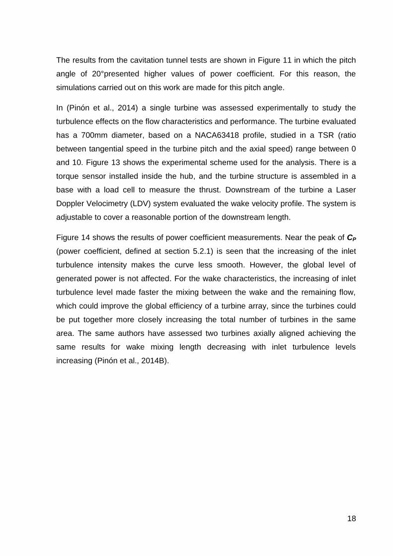
The results from the cavitation tunnel tests are shown in Figure 11 in which the pitch
angle of 20°presented higher values of power coefficient. For this reason, the
simulations carried out on this work are made for this pitch angle.
In (Pinón et al., 2014) a single turbine was assessed experimentally to study the
turbulence effects on the flow characteristics and performance. The turbine evaluated
has a 700mm diameter, based on a NACA63418 profile, studied in a TSR (ratio
between tangential speed in the turbine pitch and the axial speed) range between 0
and 10. Figure 13 shows the experimental scheme used for the analysis. There is a
torque sensor installed inside the hub, and the turbine structure is assembled in a
base with a load cell to measure the thrust. Downstream of the turbine a Laser
Doppler Velocimetry (LDV) system evaluated the wake velocity profile. The system is
adjustable to cover a reasonable portion of the downstream length.
Figure 14 shows the results of power coefficient measurements. Near the peak of CP
(power coefficient, defined at section 5.2.1) is seen that the increasing of the inlet
turbulence intensity makes the curve less smooth. However, the global level of
generated power is not affected. For the wake characteristics, the increasing of inlet
turbulence level made faster the mixing between the wake and the remaining flow,
which could improve the global efficiency of a turbine array, since the turbines could
be put together more closely increasing the total number of turbines in the same
area. The same authors have assessed two turbines axially aligned achieving the
same results for wake mixing length decreasing with inlet turbulence levels
increasing (Pinón et al., 2014B).

19
Figure 13 – The Experimental scheme for evaluating the turbulence effects on flow through a tidal current turbine
Source: (Pinón et al., 2014)
Figure 14 - Results from power (Top Figures) and thrust (Bottom Figures) measurements with different inlet turbulence intensities - 3% on Left and 5% on Right
Source: (Pinón et al., 2014)
20
3.1.2 Computational Fluid Dynamics Analysis
(Bir et al., 2011) performed a one-way Fluid Structure Analysis with the pressure data
imported from CFD to the structural analysis. The authors used a 180° model for a
two-blade turbine, with the horizontal plane as symmetry plane. Effects due to free
surface and seabed could not be analysed with such simplification in the model. The
mesh consisted in approximately 3x10⁶ elements with higher refinement close to the
blades. With these results, the external shape of the blade was maintained, and the
internal structural design was optimized following buckling and stress criterion.
(Lloyd et al., 2011) studied the turbine from (Bahaj, W.M.J., & McCann, 2007) and
employed a numerical simulation. The GGI technique was used with an open source
CFD code (OpenFOAM) to analyse the hydrodynamic performance of the turbine. A
transient analysis, using k-ω-SST turbulence model with SIMPLE algorithm for
couple pressure and velocity was used. The mesh consists in approximately 7.105
hexahedral elements. The work did not present full convergence of the model and
the domain length used for the analysis was shown to be short. The work
underpredicted the power generated by the turbine.
(Afgan et al., 2012) compared two approaches for turbulence modelling in tidal
current turbines. For code validation, a standard k-ω-SST was used and then, a
more robust LES code was implemented to make a comparison. The simulations
were carried using the geometry from (Bahaj, W.M.J., & McCann, 2007). A mesh
sensitivity analysis was performed for the LES turbulence model, choosing a mesh
with 7.4 x 10⁶ volumes. The authors found that the differences in pressure distribution
between blades pressure and suction sides lead to an underprediction of thrust and
power coefficients. However, for TSR near the peak of CP values, both turbulence
models achieved close results with the experimental analysis. The work has
neglected the free surface effects, even on the transient analysis.
(Gebreslassie et al., 2012) performed a CFD analysis of a turbine modeled as
momentum source, generating only lift and drag, with results provided by a Hybrid
BEMT-CFD methodology to reduce computational cost. The authors performed a 3D
simulation with the OpenFOAM CFD package. This CFD model was compared with
an analytical proposal to model wake interactions trough factors based on linear

21
actuator disk model. The main conclusion of the work is that a distance of 20
diameters between two turbines is sufficient for each turbine to achieve at least 91%
of its individual power.
(Mason-Jones et al., 2012) the hydrodynamic performance of the turbine is assessed
for a non-uniform profile flow at the inlet. The data from profiled flow was obtained
from measurements made at site. The text is based on the hypothesis that the power
coefficient is function of Reynolds number and TSR value, neglecting the influence of
free surface effects. The CFD analysis was carried out with RANS equations with the
Reynolds Stress transport turbulence model. A Moving Reference Frame (MFR)
technique was applied to take the rotational effects in account,. The mesh was
refined near the blade region to achieve a y+ of 300 that has shown mesh
convergence of the results. The domain size in the streamwise direction was 10
diameters in upstream direction and 40 diameters in the downstream direction. The
CFD with a uniform profiled flow was validated with experimental measurements,
showing a good agreement between numerical and test results for a TSR range
between 5 and 6. The conclusion of the work is that both power and thrust
coefficients are independent from Reynolds number greater than 3x10⁵, allowing
experimental and numerical results based on test scale be scaled without corrections
in Reynolds number once the inlet velocity profile is correctly represented.
(Pinón et al., 2012) used a particle method instead of the Finite Volume Method for
domain discretization. The method uses a lagrangian description of the velocity field
and, in this case, no turbulence or viscous effects was considered. The blades were
modeled as vortex panels. The method had a good agreement for low TSR values,
however, near to the peak of Power coefficient, the numerical results overpredicted
the performance of the turbine. It occurs due to the misprediction of flow
characteristics as separation that limits the lift generated in the turbine blades.
However, for wake characterization, both quantitative and qualitative analysis have
shown good results.
(Sharma et al., 2013) analysed the data from a site located in the United Kingdom,
from an area sheltered from large surface waves and with currents in the order of
2.5m/s was analysed. The data consisted of velocities on the streamwise, transversal
and vertical directions in time, providing realistic turbulence measurements. It was

22
found high turbulence levels with approximately 12% of intensity with respect to the
streamwise mean velocity, 9% to the transversal velocity and 7% to the vertical
direction.
(Biskup et al., 2014) dealt with the problem of fluid structure interaction in tidal
current turbines and highlight the high computational costs for a complete simulation
within the full CFD analysis of the problem (including the rotor and the complete
structural analysis with the required mesh refinement ensuring the correct calculation
of stress gradients in the complex geometric transitions from the turbine blade). The
authors proposed a multibody analysis of the problem instead of a full modelling of
the structure. The results were fairly accurate, however, an experimental approach
was still required for the complete validation of the problem.
(Blackmore et al., 2014) analysed the influence of varying inlet turbulence intensity
on the wake characteristics of the turbine. The turbine was modeled as a momentum
source and a LES method was used to model the turbulence, based on the
Smagorinsky traditional approach. For initial condition, a pre-simulation using RANS
equations was performed. They concluded that the turbulence intensity accelerates
the wake recovery, improving the global performance of an array of turbines.
(Masters et al., 2015) compared a full-CFD approach with BEMT and the hybrid
method BEM-CFD for analyse the flow through a tidal current turbine. The boundary
layer due to the seabed shear effects was considered. For the lateral walls and free
surface, a symmetry condition was applied simulating free slip walls. The domain size
was chosen to ensure low blockage effects on the turbine. The same model was
constructed for the BEM-CFD approach, with a mesh with approximately 3x10⁶
elements. The simulations were carried out with the k- ε turbulence model. The
comparison between the results have shown a good agreement between the two
results for power, thrust and even wake profile. A BEMT model was employed to
calculate the power and thrust, revealing an underprediction of 5.4% in comparison
with BEM-CFD. That paper also presented modelling of the coastal area with
obstacles in the flow, now modelling the turbine as a porous disk in order to obtain
the velocity distribution in the turbine region inlet. A full model considering the turbine
geometry and the environment is still prohibitive, as far as computational costs are
concerned.

23
(Morris et al., 2016) performed a CFD analysis for turbines with two, three and four
blades. The parameter of analysis is the Swirl number, 𝑆𝜙, which is the ratio between
angular momentum flux and axial momentum flux, according to the equations ( 3.1 ),
( 3.2 ) and ( 3.3 ). For the CFD, they employed a domain with 10D for the upstream
length and 30 D for the downstream length (where D is the rotor diameter), with
2x10⁶ elements composing the mesh. No free surface effects were considered. The
researchers found a positive correlation between the number of blades (associated
with the solidity of the rotor disk), and the swirl number. However, the results showed
that the swirl number for tidal current turbines is low and presents a fast decay, which
means that the increasing in the tangential velocities compared with axial velocities is
small a, d therefore the wake will mix with the flow faster
𝑆𝜙 =𝐺𝜙
𝐺𝑧𝑅 ( 3.1 )
𝐺𝜙 = ∫(𝑢𝜙𝑟)𝜌𝑢𝑧 . 2. 𝜋. 𝑟. 𝑑𝑟
𝑅
0
( 3.2 )
𝐺𝑧 = ∫(𝑢𝑧 . 𝜌. 𝑢𝑧 + 𝑝. )2. 𝜋. 𝑟. 𝑑𝑟
𝑅
0
( 3.3 )
Where:
𝑆𝜙 Is the Swirl number;
𝐺𝜙 Is the tangential momentum flux through the turbine disk;
𝐺𝑧 Is the axial momentum flux through the turbine disk;
𝑅 Is the turbine disk radius;
𝑢𝜙 Is the tangential velocity;
𝑢𝑧 Is the axial velocity.
(Tatum et al., 2016) considered the effects of surface gravity waves and varying
profile flows in their study. The velocity profile was considered as a power from the
height measured from the lower boundary. The turbine was modeled in its full scale.
The work was conducted using the k-ω-SST turbulence model, and the simulation
was performed with the commercial code ANSYS CFX. The free surface was

24
resolved by the Volume of Fluid (VOF) method, which required a high refinement of
the mesh close to the free surface. The waves used in the simulation were modeled
through potential wave theory for finite depths. The conclusion of the work is the high
alternating stress caused due to gravity waves induced velocities. Both power and
thrust have oscillated in the order of 10% of its mean value, which is supposed to
cause electrical grid instabilities.
(Kulkarni et. al, 2016) studied the mesh dependency on results of steady-state
simulations of the flow through a horizontal axis tidal current turbine. In the study,
they used a full-scale turbine model, with a blade radius of 7.4m, based on a
NACA0018 profile, reaching a mesh with 2440439 nodes.
(Zhang et al., 2017) compared the wake profiles at the inlet and wave characteristics
measured in an experimental flume and compared with results obtained with a CFD
analysis. The commercial code ANSYS Fluent 18.0 was used for the numerical
analysis that was performed with RANS equations with k-ω-SST turbulence model.
The mesh convergence study pointed out to a mesh with approximately 5x10⁶
elements. The free surface was modeled as a free slip wall since the experiments did
not present a significant head difference between upstream and downstream regions
of the flow. The numerical analysis agreed with the results obtained from the
experiments regarding thrust and torque coefficients. For the far-wake velocity profile
measurements, CFD also presented good results also, validating the numerical
method.
In Table 1 the works described above in this section are summarized highlighting the
turbulence model, domain size, model used for free surface, the goals of the work
and main results.

25
Table 1 - Summary of CFD works on tidal current turbines
Reference Turbulence
Model
Domain Size
Mesh Free Surface
Model Simulation Objectives & Results
Bir et al. (2011) k-ω-SST Not
informed Not
informed No free surface
Structural analysis and pressure distribution on blades.
Lloyd et al. (2011) k-ω-SST Not
informed 7x10⁵ elem.
No free surface
GGI analysis. The transient analysis did not converge.
Afgan et al. (2012) k-ω-SST &
LES
Not informed
7.4x10⁶
elem.
No free surface
Turbulence model influence on results. They concluded that k-ω-SST is valid for CP (power coefficient) calculation,
Gebreslassie et al.
(2012) LES
L = 51 D
B = 25.3 D
H = 10.3 D
Not informed
VOF Method
Comparison of an analytical method for wake velocity modelling with CFD analysis with full blade resolved. The analytical results were close to the CFD results.
Mason-Jones et al. (2012)
Reynolds Stress
Transport
L = 50D
B = 5D
H = 5D
9.7x10⁵
MRF Free-Slip wall
Effects of inlet varying profiled flow in the performance characteristics and analyse the RE dependence on Results. They found that above the results are independent for RE > 3x10⁵.
Pinón et al. (2012) No
turbulence effects
Not informed
Not
informed No free surface
Evaluate the tidal current turbine performance without viscosity and turbulence. The analysis overpredicted the generated power even with a good agreement concerning the wake profile.

26
Reference Turbulence
Model
Domain Size
Mesh Free Surface
Model Simulation Objectives & Results
Sharma et al. (2013)
Not informed Not
informed Not
informed No free surface
Experimental assessment of the turbulent intensity at the site. Realistic turbulence intensity levels for model calibration with 12% of intensity in the streamwise direction, 9% in the transversal direction and 7% in the vertical direction.
Biskup et al. (2014)
k-ω-SST Not
informed Not
informed No free surface
The authors validated a multibody approach for fluid-structure interaction instead of full structural analysis of turbine blades.
Blackmore et al. (2014)
LES
Depends on grid
inlet
Not informed
Free-Slip wall
Evaluate the effects of inlet turbulence intensity on the wake profile. The results are similar to these found by other authors in which the increase in turbulence levels decreases the wake mixing length.
Masters et al. (2015)
k- ε Not
informed 3x10⁶ Free-Slip wall
Compares the results for full-blade resolved CFD, BEM-CFD and BEMT. All methodologies presented a good agreement with experimental results. BEMT underpredicts the peak power coefficient.
Morris et al. (2016) Reynolds
Stress Transport
L = 40D
B = 5D
H = 5D
2x10⁶ No free surface
Evaluate the turbine swirl and its relation to the number of blades. The results pointed in a low swirl number for this kind of turbine and the dependence between blades number and swirl number.

27
Reference Turbulence
Model
Domain Size
Mesh Free Surface
Model Simulation Objectives & Results
Tatum et al. (2016) k-ω-SST Not
informed 2.8x10⁶ VOF
Non-uniform inlet velocity profile and free surface waves were introduced in the boundary conditions to evaluate their results on the hydrodynamic performance. Oscillations in power and thrust were found for the flow with the effect of gravity waves.
Kulkarni et al. (2016)
k-ω-SST k-ε RNG
Not informed
2.4x10⁵ No free surface
The authors performed a mesh convergence analysis of two different two equations turbulence models. They concluded that k-ω-SST provides a better numerical prediction of the hydrodynamic performance.
Zhang et al. (2017) k-ω-SST
L = 211 D
B =4.4 D
H = 2 D
5x10⁶ Free-Slip wall
The work analysed the wake from tidal current turbines with full resolved blades. The wake profile has deviated from experimental predictions. The authors justify it due to the limitations of the turbulence model.
Where L is the domain Length, B, the domain width, H the domain Height and D is the turbine Diameter;

28
3.1.3 Analytical models
(Garret & Cummins, 2007) presented an actuator disk model to take into account the
effects of blockage. The turbine was fully confined and with no influence of free
surface effects. The authors showed that the power coefficient overcomes the Betz
Limit (the theoretical limit of 16/27 of the power coefficient in the case of an open
flow) by a factor equal to (1-B)-2 in which the power coefficient tends to infinite as the
Blockage Ratio tends to zero. However, the model will lead to an infinite pressure
drop, which does not occur in real situations.
(Houlsby et al., 2007) further developed the model for the actuator disk model with
different boundary conditions. A first model considers the actuator disk in an open
flow, conducing to the Betz Limit. A second model confined by walls and by constant
pressure are included evaluating the effects of blockage in the hydrodynamic
performance. The last model considers an open channel flow, in which in the lower
boundary, the flow is defined by a rigid wall and in the upper boundary the as a
constant pressure wall.
(Peiró et al., 2007) proposed a different scheme from (Houlsby et al., 2007) to model
an open channel actuator disk model equations. They proposed a potential model for
the interaction between the free surface with a turbine array. The model consists of
introducing the linear wave potential in the free surface modelling the turbines as
porous barriers.
(Masters et al., 2011) used the Blade Element Momentum Theory (BEMT), including
tip and hub corrections factors to perform a blade optimization. The results were
compared those obtained with a commercial code for tidal current turbines and the
original Lifting Line Theory. The results showed a good agreement.
(Galloway et al., 2011) proposed a modified version of the BEMT including the
velocity field generated by waves in the inlet velocity, carrying out a traditional
method to calculate thrust and torque coefficients. The authors have performed a
transient analysis which concluded that power fluctuations could represent an issue
for the power conversion mechanisms even without significant changes in the total
amount of generated power. Besides, for the turbine structure, the cyclical loads

29
could lead to fatigue failure. Thus, this load must be taken into account during the
turbine design.
(Estafahani & Karbasian, 2012) the authors highlight the similarity between the
physics of axial tidal current wind turbines. The formulation is based on the Blade
Element Momentum Theory. The shape of the blades is optimized pursuing the
maximum ratio between lift and drag for each section. They do not refer to any
known optimization technique based on an objective function subjected to
restrictions.
3.1.4 Tidal farm and wind farm optimization methods
The distribution of turbines in a tidal or wind farm may follow similar position that the
obtained from the optimization methods.
(Piggott et al., 2014A) approached the optimization problem is based on a two-
dimensional CFD approach, varying the number of turbines and the channel shape.
The turbine is modeled as a friction constructed from bump functions. The objective
function to be optimized is the total averaged power which is proportional to the
velocity cubed. The optimization algorithm is based on gradients.
(Piggott et al., 2014B) presented a comparison between the methods for optimizing a
tidal-current farm for maximum power generation. The importance of this work is that
an increase of the model fidelity could lead to unfeasible computational costs. For
example, fully resolved blade simulation which produces accurate results are
expensive even for a single turbine simulation.
(Forinash & DuPont, 2016) proposed an optimization algorithm for offshore wind
power plants. They introduced the total cost of the wind turbine farm as the objective
function to optimize the difference between the total cost and the profit from the
energy sold to the electricity grid. In order to determine the power generated by each
turbine, they used an analytical model with wake propagation. The number of
turbines and their position were the design variables.
(Stansby & Stallard, 2016) employed an experimental analysis of a tidal current
turbine to evaluate the velocity profile at the wake. They provided an empirical
formulation for the mean wake velocity, width and velocity profile.

30
Hence, the power is proportional to the third power of the axial velocity, which is
considered the velocity distribution along the rotor radius. The objective function is
the total power generated by the turbine array, and the algorithm is based on the
gradient of the power function. The authors highlighted that the blockage effects were
estimated, but still require a further improvement for a better prediction.
The analysed papers showed that the computationally feasible methodologies for
optimizing tidal current turbine and wind turbine farm power generation is based on
the actuator disk models, even when CFD was used. Hence, the agreement between
the analytical models for a single turbine with the real velocity profiles and the power
generation is mandatory for the accuracy of the optimization models.
3.2 Open channel models
(Ferziger & Peric, 2002) divided the methods for free surface computational analysis
in surface capturing and in surface tracking. The first method includes the VOF
approach, in which the position of the free surface position is estimated based on the
proportion of water and air on each cell. In the surface tracking method, it is
necessary to obtain a height function for the interface. The authors proposed a
function based on the kinematic condition for free surface waves based mainly on the
flow direction that must remain tangent to the free surface to ensure that no mass
flux occurs through the free surface streamline.
(Battaglia et al., 2004) analysed the free surface flow with the Finite Element Method
approach. A lagrangian scheme is used for the free surface, tracking its movement
and updating the mesh in every iteration. The boundary conditions at the free surface
are forced atmospheric pressure on free surface and no tangential stresses in the
free surface.
For mesh updating, they considered that the mesh is contained in an elastic body
and the mesh moves according to the body displacement field due to its strain. A
smoothing algorithm is introduced for the free surface to adjust diffusivity. The paper
validated the methodology with 2D and 3D viscous sloshing models, and both
frequency and viscous damping were accurately predicted.

31
(Reichl et al., 2005) investigated the flow around a cylinder close to a free surface
employing a CFD with a VOF approach in a transient analysis. During the analysis, it
was found that for a Froude number close to 0.4 the non-linear phenomena of wave
braking started to appear. It is proposed a local Froude number analysis considering
the mean velocity between the obstacle and the free surface. The goal of the
analysis is studying the Strouhal number behaviour with the free surface proximity
(Mattavo & Assi, 2017) proposed an alternative methodology for free surface
treatment which was tested with the flow around a circular cylinder. Results were
compared with the obtained with VOF methodology. This model is based on potential
energy conservation substituting the gravity potential energy by the elastic potential
energy obtained through an elastic wall from a Fluid-Structure Interaction approach
between the fluid domain and a solid domain containing an orthotropic body model.

32
Chapter 4. Theoretical Fundamentals
This chapter presents the theoretical fundamentals that are necessary to perform a
CFD analysis of an axial tidal current turbine and model the elastic free surface by
coupling an orthotropic elastic body.
The CFD methodology is based on Finite Volume Method and solves the Reynolds
Averaged Navier-Stokes equations. Therefore, it is presented a review of the
equations for a viscous, incompressible and turbulent fluid flow. Besides, a brief
discussion about turbulence models is performed, since the correct chose of the
methodology is fundamental for an accurate simulation.
The potential fluid flow theory is introduced since a theoretical analysis of potential
fluid flow through a circular cylinder close to a free surface is performed using an
elastic-free surface boundary condition. Besides, the gravity wave theory lies in the
potential fluid flow theory. Therefore, the introduction of its basics concepts is
mandatory.
Still, on fluid mechanics, the integral equations for fluid mechanics are introduced.
There is a classic approach for axial turbines based on the one-dimension fluid flow
and using the balance between mass, momentum, and energy to estimate the power
and thrust generated in a turbine. For this balance, the computation of the integral
quantities in several sections of the fluid flow is necessary, justifying the presentation
of such equations.
The solid mechanics review is based on Theory of Elasticity applied for orthotropic
solid bodies. The free surface is simulated as a free-slip elastic wall. In order to
provide to this wall a stiffness independent of the position is necessary that the solid
not transmit shear stresses. Hence, the orthotropic solid is required instead of the
classical isotropic solid modeled originally in the classical Theory of Elasticity. The
section 4.3 includes the basic equations for Theory of Elasticity, the definition of
Airy’s stress function and the derivation of the differential equation for an orthotropic
solid with a negligible shear modulus.

33
Finally, a finite volume method and finite element method review are included. In this
section, only the basics of both theories are presented, and the details of the
elements used in the simulations are provided in the Attachment.
4.1 Basics equations of Fluid Dynamics
The flow through an axial tidal current turbine is commonly modeled as a viscous,
incompressible and fully turbulent flow. Some authors use potential methodologies,
which considers the viscosity within theoretical assumptions such as the Kutta
Condition that states the fluid velocity is finite in an airfoil trailing edge, and then
distributes vortex and sources in the blade surfaces. However, this work is based on
viscous, turbulent and incompressible fluid flow.
An incompressible and viscous fluid flow is governed, for a Newtonian fluid, by the
Navier-Stokes equations, and by the mass conservation equation. The Navier-Stokes
equations represent the conservation of the momentum, in which the left hand of the
equation represents the acceleration of a fluid particle and the right hand represents
the surface and body forces actuating in this fluid particle. The equation is written
below:
𝜕
𝜕𝑡(𝑢𝑖) +
𝜕
𝜕𝑥𝑗(𝑢𝑖𝑢𝑗) = −
1
𝜌
𝜕𝑝
𝜕𝑥𝑖+
𝜕
𝜕𝑥𝑗(𝜈
𝜕𝑢𝑖
𝜕𝑥𝑗) + 𝑔𝑖 ( 4.1 )
Where:
𝑢𝑖 Is the velocity vector;
𝜌 Is the fluid density;
𝑝 Is the fluid pressure;
𝜈 Is the fluid kinematic viscosity;
𝑔𝑖 Is the gravity acceleration.
The mass conservation equation for a continuous media is written below:
𝜕
𝜕𝑡(𝜌) +
𝜕
𝜕𝑥𝑖
(𝜌𝑢𝑖) = 0 ( 4.2 )

34
If the fluid is incompressible, the density is constant along the time, which means that
the volume of a fluid particle must remain constant during the flow, which is written by
the following equation:
𝜕
𝜕𝑥𝑖
(𝑢𝑖) = 0 ( 4.3 )
The presented equations apply for both laminar and turbulent flows. However, due to
the nature of a turbulent flow which is characterized by an aleatory motion of the fluid
particles. A high mesh is required for tracking their position, being unfeasible for most
of the industrial fluid flow analysis. A common approach is to model a turbulent flow
by their main quantities, and in this approach, a variable is divided into two parts, as
follows in the equation below:
𝜑 = �̅� + 𝜑′ ( 4.4 )
Where:
𝜑 Is a generic quantity;
�̅� Is the mean of this generic quantity;
𝜑′ Is the fluctuation of this generic quantity;
As property of the division of a generic quantity in a mean and a fluctuation parts,
follows that both means of the fluctuation part and fluctuation of a mean part are
equal to zero, which are represented by the following equations:
(�̅�)′ = 0 ( 4.5 )
(𝜑′)̅̅ ̅̅ ̅̅ = 0 ( 4.6 )
Applying the division of the velocity and pressure in the Navier-Stokes equations and
the mass conservation equation for an incompressible fluid flow and by taking the
mean of both equations is derived the Reynolds Averaged Navier Stokes (RANS)
equations which are written by:
𝜕�̅�𝑖
𝜕𝑡+
𝜕(�̅�𝑖�̅�𝑗)
𝜕𝑥𝑗= −
1
𝜌
𝜕p̅
𝜕𝑥𝑖+ 𝑔𝑖 +
𝜕
𝜕𝑥𝑗(𝜈
𝜕�̅�𝑖
𝜕𝑥𝑗− u𝑖
′u𝑗′̅̅ ̅̅ ̅) ( 4.7 )
𝜕�̅�𝑖
𝜕𝑥𝑖= 0 ( 4.8 )

35
Where:
�̅�𝑖 Is the mean velocity vector;
p̅ Is the mean fluid pressure;
−u𝑖′u𝑗
′̅̅ ̅̅ ̅ Is the Reynolds stress tensor.
The RANS model brings four equations (three equations from the mean velocity
vector and one equation for mean pressure) to solve ten variables (three velocity
components, mean pressure and six components from the Reynolds stress tensor).
Hence, an additional hypothesis and equations are necessary to close the problem.
In the next section, it is introduced some hypothesis as the turbulent viscosity, and
some models involving the transport of turbulent kinetic energy are used.
Hitherto it was presented only the differential equations used for turbulent, viscous
and incompressible fluid flow. However, for some analysis, an integral formulation,
computing mean values of the flow is necessary too. Using the Reynolds transport
equations, which is presented in (Munson, Young, & Okiishi, 2002, pp. 163-170), a
balance of an intensive scalar quantity 𝑞 is performed in a control volume according
to the following equation:
𝐷
𝐷𝑡∭ 𝜌𝑞𝑑∀
∀𝐶
=𝜕
𝜕𝑡∭ 𝜌𝑞𝑑∀
∀𝐶
+ ∬ 𝜌𝑞(�⃗�. �⃗⃗�)𝑑𝑆
𝑆𝑐
( 4.9 )
Where:
∀𝐶 Is the control volume;
𝑆𝑐 Is the control surface (boundaries from the control volume);
𝑞 Is an intensive scalar quantity.
This equation is usually applied to mass, momentum, angular momentum and
energy. For mass the equation becomes:
𝐷
𝐷𝑡∭ 𝜌𝑑∀
∀𝐶
=𝜕
𝜕𝑡∭ 𝜌𝑑∀
∀𝐶
+ ∬ 𝜌(�⃗�. �⃗⃗�)𝑑𝑆
𝑆𝑐
( 4.10 )

36
Considering a fixed control volume and an incompressible flow, this equation is
simplified to:
∬ 𝜌(�⃗�. �⃗⃗�)𝑑𝑆
𝑆𝑐
= 0 ( 4.11 )
Applying the equation ( 4.8 ) to the velocity vector:
𝐷
𝐷𝑡∭ 𝜌�⃗�𝑑∀
∀𝐶
=𝜕
𝜕𝑡∭ 𝜌�⃗�𝑑∀
∀𝐶
+ ∬ 𝜌�⃗�(�⃗�. �⃗⃗�)𝑑𝑆
𝑆𝑐
( 4.12 )
Considering a fixed control volume and an incompressible flow, this equation is
simplified to:
𝜌 ∬ �⃗�(�⃗�. �⃗⃗�)𝑑𝑆
𝑆𝑐
= ∑ �⃗�𝑒𝑥𝑡 ( 4.13 )
Where:
∑ �⃗�𝑒𝑥𝑡 Is the sum of external forces acting in the control volume.
Applying the equation ( 4.8 ) to the angular momentum.
𝐷
𝐷𝑡∭ 𝜌(𝑟 × �⃗�)𝑑∀
∀𝐶
=𝜕
𝜕𝑡∭ 𝜌(𝑟 × �⃗�)𝑑∀
∀𝐶
+ ∬ 𝜌(𝑟 × �⃗�)(�⃗�. �⃗⃗�)𝑑𝑆
𝑆𝑐
( 4.14 )
Considering a fixed control volume and an incompressible flow, this equation is
simplified to:
𝜌 ∬(𝑟 × �⃗�)(�⃗�. �⃗⃗�)𝑑𝑆
𝑆𝑐
= ∑ �⃗⃗⃗�𝑒𝑥𝑡 ( 4.15 )
Where:
∑ �⃗⃗⃗�𝑒𝑥𝑡 Is the sum of external moments acting in the control volume.

37
For Blade Element Momentum Theory, the velocity vector is divided into two main
components. The first component, with the streamwise direction and the second
component with tangential direction. The radial component is neglected in such
analysis. In this model, the conservation of angular momentum is performed between
the inlet and outlet sections, using only the painted control volume shown in Figure
15. Applying the equation ( 4.15 ) in this domain is obtained the rotating annular
stream tube angular momentum conservation equation:
𝑑𝑀𝑍
𝑑𝑟= 2𝜋. 𝜌. ∆𝜔. 𝑈. 𝑟3 ( 4.16 )
Where:
𝑀𝑍 Is the moment in the flow direction axis;
𝑟 Is the radius of the analyzed portion of the rotating annulus;
∆𝜔 Is the difference of angular speed between the inlet and outlet.
The integral conservation of energy is not presented in this text since the Bernoulli’s
equation with losses is applied instead of the second law of thermodynamics. The
Bernoulli’s equation between a point “i” representing the inlet and a point “o”
representing the outlet becomes:
ℎ𝑖 +𝑢𝑖
2
2𝑔+
𝑝𝑖
𝜌𝑔= ℎ𝑜 +
𝑢𝑜2
2𝑔+
𝑝𝑜
𝜌𝑔+
𝐹𝑒𝑥𝑡
𝜌𝑔𝐴 ( 4.17 )
Where:
ℎ Is the static head;
𝐹𝑒𝑥𝑡
𝜌𝑔𝐴 Is the losses between inlet and outlet due to external forces.
Figure 15 - Domain with one inlet and one outlet aligned to flow direction

38
4.1.1 Turbulence Models
In the RANS model, a term related to the velocity vector fluctuation appears in the
diffusive term from the equation. This term is called Reynolds stress tensor and is
responsible for the momentum diffusion in the flow. In turbulent flows, for example, in
regions far from the boundary layer, this term is more representative than the viscous
shear stress term, which is presented in Figure 16, comparing the viscous and
turbulent shear stresses in function of the distance from the wall. Hence, its
modelling is necessary to guarantee the accuracy of the turbulent flow analysis.
There are several turbulence modelling methods. The most complete, Direct Navier
Stokes Simulation (DNS), is computationally expensive since it simulates the
unsteady Navier-Stokes equation without the division between mean and fluctuation
components. That requires such domain and time step discretization that becomes
unfeasible most of industrial flows analysis by such method. However, using the
RANS model, there are some methods for calculating the Reynolds Stress Tensor.
Moreover, in some of these methods, such as 𝒌- 𝜺 and 𝒌- 𝝎 – SST uses the
turbulent viscosity hypothesis. It assumes that the turbulent shear stress is
proportional to the velocity component as happens for the viscous shear stress. The
turbulent viscosity hypothesis is represented by the following equation.
−u𝑖′u𝑗
′̅̅ ̅̅ ̅ = 𝜈𝑇
𝜕�̅�𝑖
𝜕𝑥𝑗 ( 4.18 )
Figure 16 - Profiles of the fractional contributions of the viscous and Reynolds stresses, from
DNS data, with dashed lines representing 𝑅𝑒 = 5600 and solid lines 𝑅𝑒 = 13750
Source: (Kim & Moser, 1987)

39
The problem for solving the Reynolds Stresses becomes simpler since it originally
has six components and now, according to this hypothesis, it is simplified to only one
variable. However, even that such assumption leads to accurate results, this
hypothesis is not physically consistent, since the turbulent shear stress proportional
to the velocity gradient is a particular case of turbulent flow. Besides that, since that
one more variable, the turbulent viscosity must be determined, at least one more
equation needs to be derived to close this mathematical model.
The section 3.1.2 highlighted the turbulent models used by other authors. Is clearly
seen that most of the works used the 𝒌- 𝝎 – SST Model, which calculates the
turbulent viscosity from the turbulent kinetic energy, 𝑘, and from the turbulent
rotational kinetic energy, 𝝎.
From the definition of the Reynolds stress tensor, it is defined by the turbulent kinetic
energy, 𝑘, which is invariant and hence independent from the coordinate system.
𝑘 =u𝑖
′u𝑖′̅̅ ̅̅ ̅
2 ( 4.19 )
The dissipation of turbulent kinetic energy is provided by the molecular viscosity. In
this text, the complete transport equation for turbulent kinetic energy is not analyzed.
However, it is found in (Wilcox, 1994, p. 74). The total amount of turbulent kinetic
energy is related to production, 𝒫, and dissipation, 휀, of turbulence. Both terms of
production and dissipation of turbulent kinetic energy are presented below:
𝒫 = −u𝑖′ u𝑗
′̅̅ ̅̅̅ ∂�̅�𝑖
∂𝑥𝑗 ( 4.20 )
휀 = 𝜈 (∂u𝑖
′
∂𝑥𝑗
∂u𝑖′
∂𝑥𝑗
)̅̅ ̅̅ ̅̅ ̅̅ ̅̅ ̅
( 4.21 )
From this equation, is seen that the production is related to the total amount of
Reynolds shear stress and the mean velocity gradient, while the dissipation is related
to the gradients of velocity fluctuations. Besides, according to the equation ( 4.18 ),
the turbulent diffusion increases with the turbulence intensity, which are related to the
balance between production and dissipation. Therefore, there is fundamental to
model those quantities with accuracy.
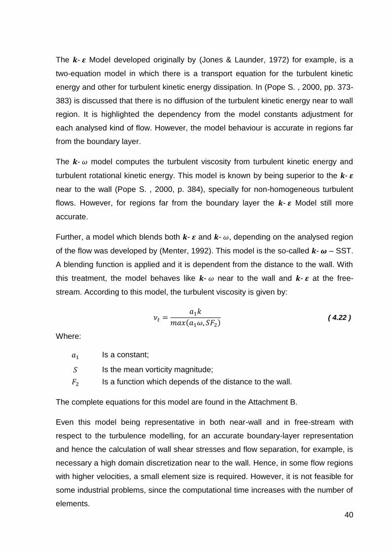
40
The 𝒌- 𝜺 Model developed originally by (Jones & Launder, 1972) for example, is a
two-equation model in which there is a transport equation for the turbulent kinetic
energy and other for turbulent kinetic energy dissipation. In (Pope S. , 2000, pp. 373-
383) is discussed that there is no diffusion of the turbulent kinetic energy near to wall
region. It is highlighted the dependency from the model constants adjustment for
each analysed kind of flow. However, the model behaviour is accurate in regions far
from the boundary layer.
The 𝒌- 𝜔 model computes the turbulent viscosity from turbulent kinetic energy and
turbulent rotational kinetic energy. This model is known by being superior to the 𝒌- 𝜺
near to the wall (Pope S. , 2000, p. 384), specially for non-homogeneous turbulent
flows. However, for regions far from the boundary layer the 𝒌- 𝜺 Model still more
accurate.
Further, a model which blends both 𝒌- 𝜺 and 𝒌- 𝜔, depending on the analysed region
of the flow was developed by (Menter, 1992). This model is the so-called 𝒌- 𝝎 – SST.
A blending function is applied and it is dependent from the distance to the wall. With
this treatment, the model behaves like 𝒌- 𝜔 near to the wall and 𝒌- 𝜺 at the free-
stream. According to this model, the turbulent viscosity is given by:
𝜈𝑡 =𝑎1𝑘
𝑚𝑎𝑥(𝑎1𝜔, 𝑆𝐹2) ( 4.22 )
Where:
𝑎1 Is a constant;
𝑆 Is the mean vorticity magnitude;
𝐹2 Is a function which depends of the distance to the wall.
The complete equations for this model are found in the Attachment B.
Even this model being representative in both near-wall and in free-stream with
respect to the turbulence modelling, for an accurate boundary-layer representation
and hence the calculation of wall shear stresses and flow separation, for example, is
necessary a high domain discretization near to the wall. Hence, in some flow regions
with higher velocities, a small element size is required. However, it is not feasible for
some industrial problems, since the computational time increases with the number of
elements.

41
In order to solve this problem, some commercial CFD codes, such as the ANSYS
CFX® which applies scalable wall functions based on (Launder & Spalding, 1974).
The complete formulation is presented in the Attachment C. In this context, it is
presented in the Figure 17 a typical profile for a turbulent boundary layer in a flat
plate. There is three different regions. The first one, called sublayer have the
predominance of molecular viscosity effects. The next region is known as Log-Layer
and comprehends a 𝑦+ between 10 and 103 approximately. The last region is known
as defect layer and represents the transition between the boundary layer and the free
stream. Usually, it is used dimensionless distances to the wall according to the
following equations:
𝜏𝑊 = 𝜌𝜈 (𝑑�̅�
𝑑𝑦)|
𝑦=0
( 4.23 )
𝑢𝜏 ≡ √𝜏𝑊
𝜌
( 4.24 )
𝑦+ =𝑢𝜏. 𝑦
𝜈 ( 4.25 )
Where:
𝜏𝑊 Is the wall viscous shear stress;
𝑢𝜏 Is the reduced velocity;
𝑦+ Is the dimensionless wall distance.
Figure 17 - Typical velocity profile for a turbulent boundary layer
Author: (Wilcox, 1994, pp. 41-53)

42
4.2 Potential Fluid Flow
For some special cases, the fluid flow could be considered as potential. When the
vorticity of the flow and hence the shear stresses are negligible, the Navier-Stokes
equation could be simplified, becoming the Poisson equation. In (Newman, 1977, p.
102) one can consider this hypothesis valid far from a thin boundary layer compared
with the dimensions involved in the analysis in which the bulk of the fluid is treated as
inviscid and irrotational.
The potential fluid flow theory yields a large amount of known analytical solutions,
such as the developed for wing and airfoils (Pope A. , 1951B), surface gravity waves,
added mass calculation and some other applications. This text includes in
Attachment the surface gravity waves theory and the potential fluid flow through a
circular cylinder, both derived with the potential fluid flow theory. The first one is
necessary to discuss the boundary conditions for a free surface and the second one
is a case with a known analytical solution that is used for analysing the effects of the
modification of the free surface boundary conditions.
According to the potential fluid flow theory, the velocity vector is derived from a
potential function, 𝜙, in which:
𝑢𝑖 =𝜕𝜙
𝜕𝑥𝑖 ( 4.26 )
Introducing this definition in the mass conservation equation, is derived the Laplace’s
equation that governs the potential fluid flow:
𝜕2𝜙
𝜕𝑥𝑖2 = 0 ( 4.27 )
Substituting the equation ( 4.26 ) in the Navier-Stokes equation, with some algebra,
is derived the Bernoulli’s equation for the potential fluid flow, which is presented in
(Newman, 1977, p. 108) and represents the conservation of energy in the flow.
𝜕𝜙
𝜕𝑡+
1
2(
𝜕𝜙
𝜕𝑥𝑗)
2
+𝑝
𝜌+ 𝑔𝑥𝑖 = 𝐶𝑡𝑒 ( 4.28 )

43
The stream function, 𝜓, represents the tangent line to a particle, such as a contour
line. The gradient of a stream function is always perpendicular to the velocity vector
and this definition is valid for any kind of flow, not only the potential fluid flow.
However, for a potential fluid flow, the stream function yields an important
mathematical property: Is the conjugate of the potential function, letting to introduce
the notion of a complex potential and therefore, the properties of the analytical
functions. With the definition of the stream function, the velocity vector is written as:
𝑢𝑖 =𝜕𝜓
𝜕𝑥𝑗𝜖𝑖𝑗𝑘 ( 4.29 )
The complex potential function, 𝐹(𝑧), is introduced, in which the potential function, 𝜙,
is the real part of the complex potential function and the streamline is the imaginary
part of the complex potential function, as follows:
𝐹(𝑧) = 𝜙(𝑥, 𝑦) + 𝑖 𝜓(𝑥, 𝑦) ( 4.30 )
Where:
𝑧 Is a complex number 𝑧 = 𝑥 + 𝑖𝑦;
𝑖 Is the imaginary number (𝑖2 = −1).
The introduction of the complex potential function allows the usage of conformal
mapping, useful for deriving the potential fluid flow through solid bodies.

44
4.3 Solid Mechanics for Orthotropic Bodies
An alternative for a free surface model, proposed by (Mattavo & Assi, 2017) employs
an orthotropic solid to evaluate the free surface effects in the flow around a circular
cylinder. They proposed that the same restoring effect could be achieved using a
mechanical spring effect instead of the gravity force. Hence, the basics of solid
mechanics for orthotropic bodies is reviewed.
The following Equation is valid for any continuous media. It states the equilibrium
between the inertia and forces and is known as Newton’s second law for particles.
The left hand of the Equation represents the inertial term and the right hand
represents the sum between body forces and surface forces. In this analysis, only
conservative body forces are considered, hence, they are derived from a potential
function.
𝜌𝜕2 𝑢𝑖
𝜕𝑡2=
𝜕𝒱
𝜕𝑥𝑖+
𝜕𝜏𝑖𝑗
𝜕𝑥𝑗 ( 4.31 )
Where:
𝑢𝑖 Is the displacement of the particles in a Lagrangian reference frame;
𝒱 Is the body force potential;
𝜏𝑖𝑗 Is the stress tensor.
Defining the strain tensor as the gradient of the displacement vector and
decomposing it in two parts, one symmetric, called strain tensor, and the other
antisymmetric, called infinitesimal rotation tensor.
𝜕𝑢𝑖
𝜕𝑥𝑗= �̃�𝑖𝑗 + �̃�𝑖𝑗 =
1
2(
𝜕𝑢𝑖
𝜕𝑥𝑗+
𝜕𝑢𝑗
𝜕𝑥𝑖) +
1
2(
𝜕𝑢𝑖
𝜕𝑥𝑗−
𝑢𝑗
𝜕𝑥𝑖) ( 4.32 )
Where:
�̃�𝑖𝑗, Is the strain tensor;
�̃�𝑖𝑗 Is the infinitesimal rotation tensor.

45
In linear elastic bodies, only the �̃�𝑖𝑗 is taken in account. For a general solid, there is a
constitutive equation that relates stress and strain and it is found in (Lai, Krempl, &
Ruben, 2010, p. 204) and is written below:
𝜏𝑖𝑗 = 𝐶𝑖𝑗𝑘𝑙 . �̃�𝑖𝑗 ( 4.33 )
Where:
𝐶𝑖𝑗𝑘𝑙 Is the stiffness tensor for a linear elastic solid.
For a linear elastic orthotropic solid, the constitutive equation is simplified. An
orthotropic material holds three orthogonal symmetry planes and this property is
applied in the stiffness tensor. The strain tensor could be divided in two parts:
elongation strain and shearing strain, as follows in the equations below:
휀𝑖 =𝜕𝑢𝑖
𝜕𝑥𝑖 ( 4.34 )
𝛾𝑖𝑗 =𝜕𝑢𝑖
𝜕𝑥𝑗+
𝜕𝑢𝑗
𝜕𝑥𝑖 ( 4.35 )
Where:
휀𝑖 Is the elongation strain;
𝛾𝑖𝑗 Is the shearing strain.
With the definition of elongation and shearing strain, it is possible to relate stress and
strain for an orthotropic solid material according to the equations below:
휀𝑖 = 𝛿𝑖𝑗
𝜎𝑖
𝐸𝑖+ (𝛿𝑖𝑗 − 1)
𝑢𝑖𝑗𝜎𝑗
𝐸𝑗 ( 4.36 )
𝛾𝑖𝑗 =𝜏𝑖𝑗
𝐺𝑖𝑗 ( 4.37 )
Where:
𝐸𝑖 Is the orthotropic elasticity modulus;
𝐺𝑖𝑗 Is the shear modulus.

46
For a two-dimensional problem, It is defined too the Airy’s stress function, Φ𝐴,
according to (Timoshenko & Goodier, 2010, pp. 31-33). All stress components are
derived from this single function. Therefore, it yields a mathematical advantage in the
solid mechanics problems solving, since just a single function must be found. For
transient analysis, a modification in the definition of stresses is performed, including a
term related to the second derivative with respect to the time in its definition, shown
in (Timoshenko & Goodier, 2010, pp. 485-513).
𝜎𝑥 =𝜕2Φ𝐴
𝜕𝑧2+ 𝒱 + 𝜌
𝜕2Φ𝐷
𝜕𝑡2 ( 4.38 )
𝜎𝑧 =𝜕2Φ𝐴
𝜕𝑥2+ 𝒱 + 𝜌
𝜕2Φ𝐷
𝜕𝑡2 ( 4.39 )
𝜏𝑥𝑧 = −𝜕2Φ𝐴
𝜕𝑥𝜕𝑧 ( 4.40 )
Where:
Φ𝐷 Is the inertial potential.
For a two-dimensional approach, only the displacements in the xz plane are
considered, leading to a plane state of displacements. For this case, the boundary
conditions are: 휀𝑦 = 𝛾𝑥𝑦 = 𝛾𝑦𝑧 = 0. Hence, is possible to write the stress in y direction
in function of stresses in x and z directions. By the substitution of these results in the
Equation ( 4.36 ) is shown that:
휀𝑥 = (1 − 𝜐𝑥𝑦2 )
𝜎𝑥
𝐸𝑥+ (𝜐𝑦𝑧𝜐𝑥𝑦 − 𝜐𝑥𝑧)
𝜎𝑧
𝐸𝑧 ( 4.41 )
휀𝑧 = (1 − 𝜐𝑦𝑧2 )
𝜎𝑧
𝐸𝑧+ (𝜐𝑦𝑧𝜐𝑥𝑦 − 𝜐𝑥𝑧)
𝜎𝑥
𝐸𝑥 ( 4.42 )
It is possible to relate the linear strain components with the shear strain components
from the definition of 휀𝑖 and 𝛾𝑖𝑗 according to the equations ( 4.34 ) and ( 4.35 ). By
deriving twice 휀𝑖 with respect to 𝑥𝑗 and deriving twice 휀𝑗 with respect to 𝑥𝑖 and
summing these two components, it is deduced the following expression:
𝜕2휀𝑖
𝜕𝑥𝑗2 +
𝜕2휀𝑗
𝜕𝑥𝑖2 =
𝜕3𝑢𝑖
𝜕𝑥𝑖𝜕𝑥𝑗2 +
𝜕3𝑢𝑗
𝜕𝑥𝑖2𝜕𝑥𝑗
( 4.43 )

47
The same expression is obtained by deriving the expression ( 4.35 ).one time with
respect to 𝑥𝑖 and once with respect to 𝑥𝑗. Hence, is derived an expression relating the
strain components 휀𝑖 and 휀𝑗 with 𝛾𝑖𝑗. Since the analysis focuses on a two-dimensional
state of deformations, the following expression relates 휀𝑥 and 휀𝑧 with 𝛾𝑥𝑧.
𝜕2휀𝑥
𝜕𝑧2+
𝜕2휀𝑧
𝜕𝑥2=
𝜕2𝛾𝑥𝑧
𝜕𝑥𝜕𝑧 ( 4.44 )
Substituting the expression. ( 4.37 ) for 𝛾𝑥𝑧, ( 4.41 ) for 휀𝑥 and ( 4.42 ) for 휀𝑧 in the
equation ( 4.44 ), it is obtained the following equation, relating 𝜎𝑥 and 𝜎𝑧 with 𝜏𝑥𝑧.:
𝜕2
𝜕𝑧2[(1 − 𝜐𝑥𝑦
2 )𝜎𝑥
𝐸𝑥+ (𝜐𝑦𝑧𝜐𝑥𝑦 − 𝜐𝑥𝑧)
𝜎𝑧
𝐸𝑧]
+𝜕2
𝜕𝑥2[(1 − 𝜐𝑦𝑧
2 )𝜎𝑧
𝐸𝑧+ (𝜐𝑦𝑧𝜐𝑥𝑦 − 𝜐𝑥𝑧)
𝜎𝑥
𝐸𝑥] =
𝜕2
𝜕𝑥𝜕𝑧(
𝜏𝑥𝑧
𝐺𝑥𝑧)
( 4.45 )
Substituting the stresses by its definition based on modified Airy’s stress function,
according to ( 4.38 ), ( 4.39 ) and ( 4.40 ), and rearranging the terms is deduced the
differential equation for Airy’s stress function in orthotropic solids.
(1 − 𝜐𝑥𝑦2 )
𝐸𝑥
𝜕4Φ𝐴
𝜕𝑧4+ [
1
𝐺𝑥𝑧− (𝜐𝑦𝑧𝜐𝑥𝑦 − 𝜐𝑥𝑧) (
1
𝐸𝑥+
1
𝐸𝑧)]
𝜕4Φ𝐴
𝜕𝑥2𝜕𝑧2+
(1 − 𝜐𝑦𝑧2 )
𝐸𝑧
𝜕4Φ𝐴
𝜕𝑥4
= − {[(1 − 𝜐𝑥𝑦
2 )
𝐸𝑥−
(𝜐𝑦𝑧𝜐𝑥𝑦 − 𝜐𝑥𝑧)
𝐸𝑧]
𝜕2
𝜕𝑧2
+ [(1 − 𝜐𝑦𝑧
2 )
𝐸𝑧−
(𝜐𝑦𝑧𝜐𝑥𝑦 − 𝜐𝑥𝑧)
𝐸𝑥]
𝜕2
𝜕𝑥2} (𝒱 + 𝜌
𝜕2Φ𝐷
𝜕𝑡2)
( 4.46 )
For simplicity, is defined that 𝐸𝑥 = 𝐸𝑧 = 𝐸, 𝜐𝑥𝑦 = 𝜐𝑦𝑧 = 𝜐𝑥𝑧 = 𝜐 and 𝐺𝑥𝑧 = 𝐺.
Substituting in the equation ( 4.46 ):
𝐺
𝐸(1 − 𝜐2)
𝜕4Φ𝐴
𝜕𝑧4+ [1 +
𝐺
𝐸2𝜐(1 − 𝜐)]
𝜕4Φ𝐴
𝜕𝑥2𝜕𝑧2+
𝐺
𝐸(1 − 𝜐2)
𝜕4Φ𝐴
𝜕𝑥4
= −𝐺
𝐸(1 + 𝜐 − 2𝜐2) (
𝜕2
𝜕𝑧2+
𝜕2
𝜕𝑥2) (𝒱 + 𝜌
𝜕2Φ𝐷
𝜕𝑡2)
( 4.47 )
For a solid with the shear modulus small if compared with elasticity modulus, the
equation ( 4.47 ) becomes:
𝜕4Φ𝐴
𝜕𝑥2𝜕𝑧2= 0 ( 4.48 )
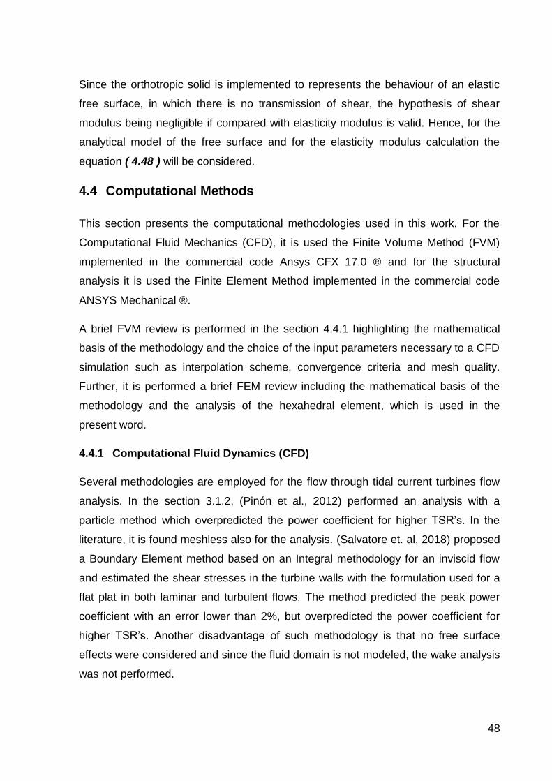
48
Since the orthotropic solid is implemented to represents the behaviour of an elastic
free surface, in which there is no transmission of shear, the hypothesis of shear
modulus being negligible if compared with elasticity modulus is valid. Hence, for the
analytical model of the free surface and for the elasticity modulus calculation the
equation ( 4.48 ) will be considered.
4.4 Computational Methods
This section presents the computational methodologies used in this work. For the
Computational Fluid Mechanics (CFD), it is used the Finite Volume Method (FVM)
implemented in the commercial code Ansys CFX 17.0 ® and for the structural
analysis it is used the Finite Element Method implemented in the commercial code
ANSYS Mechanical ®.
A brief FVM review is performed in the section 4.4.1 highlighting the mathematical
basis of the methodology and the choice of the input parameters necessary to a CFD
simulation such as interpolation scheme, convergence criteria and mesh quality.
Further, it is performed a brief FEM review including the mathematical basis of the
methodology and the analysis of the hexahedral element, which is used in the
present word.
4.4.1 Computational Fluid Dynamics (CFD)
Several methodologies are employed for the flow through tidal current turbines flow
analysis. In the section 3.1.2, (Pinón et al., 2012) performed an analysis with a
particle method which overpredicted the power coefficient for higher TSR’s. In the
literature, it is found meshless also for the analysis. (Salvatore et. al, 2018) proposed
a Boundary Element method based on an Integral methodology for an inviscid flow
and estimated the shear stresses in the turbine walls with the formulation used for a
flat plat in both laminar and turbulent flows. The method predicted the peak power
coefficient with an error lower than 2%, but overpredicted the power coefficient for
higher TSR’s. Another disadvantage of such methodology is that no free surface
effects were considered and since the fluid domain is not modeled, the wake analysis
was not performed.

49
Even with these methodologies, most of the author analysed the flow through tidal
current turbines using a Finite Volume Method, as discussed previously. With such
methodology is possible to analyse the whole fluid domain including turbulence, free
surface and confinement effects. A multiphasic flow such as the Volume of Fluid
(VOF) for free surface analysis. Hence, this methodology is applied in the present
work and is discussed in this chapter.
The equations presented in the section 4.1 could be represented in the conservative
form, as discussed in (Pantankar, 1980, pp. 15-17). In this general form, the transport
equation of a scalar quantity 𝜑 is given by:
𝜕
𝜕𝑡(𝜌𝜑) +
𝜕
𝜕𝑥𝑗(𝜌𝑢𝑗𝜑) =
𝜕
𝜕𝑥𝑗[Γ𝜑
𝜕
𝜕𝑥𝑗
(𝜑)] + 𝑆𝜑 ( 4.49 )
Where:
𝜑 Is a scalar quantity;
Γ𝜑 Is the diffusion coefficient related to this scalar quantity;
𝜕
𝜕𝑡(𝜌𝜑) Is the local rate of change;
𝜕
𝜕𝑥𝑗(𝜌𝑢𝑗𝜑) Is the advective rate of change;
𝜕
𝜕𝑥𝑗[Γ𝜑
𝜕
𝜕𝑥𝑗
(𝜑)] Is the diffusive term;
𝑆𝜑 Is the source term.
In an incompressible, viscous and turbulent flow, such the analysed in this text, using
the k-ω-SST for turbulence modelling, there are six differential equations to be solved
and all of then written in the same form as the equation ( 4.49 ). In order to solve this
mathematical problem, these equations must be discretized in order to be solved in a
finite quantity of points in the fluid domain. In (Maliska, 2014, pp. 195-196) this
equation is integrated for a general fluid element. For a node “i”, the equation
becomes:

50
Figure 18 - Control Volume Integration for Element Based Finite Volume Method
Source: (Profito, 2015)
𝑀𝑃𝜑𝑖 − 𝑀𝑃0𝜑𝑖
0
Δ𝑡= − ∑[𝜌(�⃗⃗�. �⃗⃗�)𝜑Δ𝑆]
𝑠𝑗𝑠𝑗
+ ∑[Γ𝜑(∇𝜑. �⃗⃗�)Δ𝑆]𝑠𝑗
𝑠𝑗
+ ∑(𝑆𝑖𝜑
𝜑𝑖 + 𝑆𝐶𝜑
)ΔV
𝑠𝑗
( 4.50 )
Where:
𝑀𝑃 Is the mass of the element in the analysed time step;
𝜑𝑖 Is the nodal value of 𝜑 in the node “i” in the analysed time step;
𝑀𝑃0 Is the mass of the element in the previous time step;
𝜑𝑖0 Is the nodal value of 𝜑 in the node “i” in the previous time step;
Δ𝑡 Is the time step of the integration;
�⃗⃗� Is the Velocity Vector;
�⃗⃗� Is the normal vector to a control surface;
𝑠𝑗 Is the control surface “j”;
Δ𝑆 Is the control surface total area;
𝑆𝑖𝜑
Is the source term in the node “i” in the analysed time step;
𝑆𝐶𝜑
Is the independent part of the linearized source term;
ΔV Is the total volume of the element “i”.

51
The Figure 18 illustrates the integrated domain for generating the equation ( 4.50 ).
The point “P” shown in the figure represents the node “i” used in the equation above.
Besides, for calculating the values of 𝜑 in the subdomain boundaries, represented by
𝑠𝑗 in the equation and by a thick line in the figure, is cecessary to interpolate the
value of 𝜑 using the values of this variable in the neighbour nodes. In the diffusive
term, the gradient of 𝜑 must be calculated also. Hence, the derivatives of 𝜑 must be
calculated and since they are not known a priori, a proper scheme of interpolation
shall be careful chosen.
In (Maliska, 2014, pp. 75 - 104) several interpolation functions are discussed for the
diffusive and advective components. The dependency of the dominant phenomena in
the flow is a relevant factor in the choice of the interpolation scheme. The upwind
scheme, for example, which calculates the derivative using only the upstream node
following the flow direction smooths gradients and could lead to a problem called
numerical diffusion.
Some interpolation functions consider the effects of the advective term. For example,
in a flow in which the advective transport is dominant if compared with diffusion,
which occurs in regions far from boundary layer in high Reynolds flows, the
downstream values of a certain variable 𝜑 are more representative than the
upstream and points which are not in the streamwise direction. Hence, a weighted
scheme such as Weighted Upstream Differencing Scheme – Extended (WUDS-E) is
a valuable option.
For incompressible flows, the pressure and velocity are decoupled a priori. In the
momentum conservation equation, the pressure gradient is used as a source for
calculating the velocity components. However, for calculating the pressure field, there
is not a single equation in which the pressure term could be separated. Deriving the
equation ( 4.7 ) with respect to 𝑥𝑖 is found the Poisson Equation for pressure, as
follows:
𝜕2p̅
𝜕𝑥𝑖2 = −𝜌 [
𝜕�̅�𝑖
𝜕𝑥𝑗
𝜕�̅�𝑗
𝜕𝑥𝑖+
𝜕2
𝜕𝑥𝑗𝜕𝑥𝑖(u𝑖
′u𝑗′̅̅ ̅̅ ̅)] ( 4.51 )

52
Some pressure-velocity coupling methods such as SIMPLE (Semi-Implicit Linked
Equations) and SIMPLER (Semi-Implicit Linked Equations-Revised) makes use of
Poisson equation for pressure to correct the pressure field. Besides, the most known
methods for solving a CFD problem through FVM makes use of an iterative solver.
Since the Navier-Stokes equations are not linear. Hence, the pressure-velocity
coupling methods are iterative and needs a convergence criterium.
The standard method in the commercial code ANSYS CFX 17.0® is the Fourth Order
Rhie-Chow Method (Rhie & Chow, 1982). This coupling is applied for a co-located
grid in which the control volume is the same for all transport equations. The method
uses the continuity equation to solve the pressure field.
4.4.2 Finite Element Method
The finite element method is often used for structures and heat transfer problems.
There are high order methods applied to fluids, however, this approach is not shown
in this work since the scope is limited to the Finite Element application on structures.
From (Hughes, 2000), it is known that a boundary value problem could be analysed
by a strong, differential formulation and through a weak, integral formulation. And
both methods are mathematically equivalent. The Finite Element Method uses the
integral approach for discretize the system through interpolation functions, so-called
shape functions, and provide trough integrals along the element domain, formulas for
the stiffness and load parameters that describes the system.
From (Timoshenko & Goodier, 2010, pp. 235-277), for a three dimensional elastic
solid, the differential approach for analysing the deformations came from newton
second law for infinitesimal values. This equation relates by equilibrium of forces, the
relation between stresses and body forces. Analysing the stress field in the solid
boundaries with the compatibility of strain and by the equilibrium of forces, the
deformation field along the body is found. However, this section is interested on
analyse the integral formulations of solid mechanics. From (Timoshenko & Goodier,
2010, pp. 235-277), the strain potential energy stored in an elastic body, contained in
the domain Ω𝐷, it is given by the following integral:
53
𝒰𝑠𝑡𝑟𝑎𝑖𝑛 =1
2∫ {𝜎}𝑇 . {휀}. 𝑑Ω𝐷
Ω𝐷
( 4.52 )
Where:
𝒰𝑠𝑡𝑟𝑎𝑖𝑛 Is elastic potential energy due to a solid deformation;
{𝜎} Is the stress vector;
{휀} Is the strain vector;
Ω𝐷 Is the solid domain.
For a linear elastic body, the stress and strain are related by a linear transformation.
Let [𝒟] be the matrix which contains the relation between stress and strain. The
integral becomes:
𝒰𝑠𝑡𝑟𝑎𝑖𝑛 =1
2∫ {휀}𝑇[𝒟]. {휀}. 𝑑Ω𝐷
Ω𝐷
( 4.53 )
The external forces produce an amount of work that by energy conservation must be
equal to the stored strain energy. Dividing the work due to external forces by work
due to body forces, 𝒲𝐵, and work due to surface forces, 𝒲𝑠, and calling the domain
boundary as ∂Ω𝐷, the work due to external forces is given by:
𝒲 = 𝒲𝐵 + 𝒲𝑆 = ∫ 𝑋𝑖𝑢𝑖 . 𝑑Ω𝐷
Ω𝐷
+ ∫ 𝑆𝑖𝑢𝑖. 𝑑 ∂Ω𝐷
∂Ω𝐷
( 4.54 )
Since the total work is equal to the total strain energy, the equation ( 4.53 ) is equal
to the equation ( 4.54 ).
1
2∫ {휀}𝑇[𝒟]. {휀}. 𝑑Ω𝐷
Ω𝐷
= ∫ 𝑋𝑖𝑢𝑖. 𝑑Ω𝐷
Ω𝐷
+ ∫ 𝑆𝑖𝑢𝑖 . 𝑑 ∂Ω𝐷
∂Ω𝐷
( 4.55 )
As described in the section 4.3, the strain is related to the displacement by
differential operators. However, the displacement field, 𝑢𝑖, it is not known a priori.
Hence, the domain is divided into small parts indeed, and for each part, it is given a
set of functions with value equal to zero outside the element domain, which

54
interpolates the displacement values from given nodes to calculate the displacement
inside the element domain. Calling 𝒩𝑖𝑒the set of shape functions associated with
each element, the differential operator which relates stress and strain could be turned
into an algebraic operator, [ℬ]. Hence, the equation ( 4.55 ) becomes:
1
2∫ {𝑢}𝑇[ℬ]𝑡[𝒟]. [ℬ]{𝑢}. 𝑑Ω𝐷
Ω𝐷
= ∫ 𝑋𝑖[𝒩]{𝑢}. 𝑑Ω𝐷
Ω𝐷
+ ∫ 𝑆𝑖[𝒩]{𝑢}. 𝑑 ∂Ω𝐷
∂Ω𝐷
( 4.56 )
Since the nodal displacement vector is constant, it could be taken out from the
integrals:
1
2{𝑢}𝑇 ∫[ℬ]𝑡[𝒟]. [ℬ]. 𝑑Ω𝐷
Ω𝐷
{𝑢} = {𝑢}𝑇 { ∫ 𝑋𝑖[𝒩]. 𝑑Ω𝐷
Ω𝐷
+ ∫ 𝑆𝑖[𝒩]. 𝑑 ∂Ω𝐷
∂Ω𝐷
} ( 4.57 )
According to the minimum complementary potential energy theorem, the
displacements are such that the difference between strain potential energy and
stored external work is stationary. Hence, the variational of the previous equation is
equal to zero. It yields:
{𝛿𝑢}𝑇 {[ ∫[ℬ]𝑡[𝒟]. [ℬ]. 𝑑Ω𝐷
Ω𝐷
] {𝑢} − ∫ 𝑋𝑖[𝒩]. 𝑑Ω𝐷
Ω𝐷
− ∫ 𝑆𝑖[𝒩]. 𝑑 ∂Ω𝐷
∂Ω𝐷
} = 0 ( 4.58 )
Therefore, the displacement vector must fulfil the following relation:
[ ∫ [ℬ]𝑡[𝒟]. [ℬ]. 𝑑Ω𝐷
Ω𝐷
] {𝑢} = ∫ 𝑋𝑖[𝒩]. 𝑑Ω𝐷
Ω𝐷
+ ∫ 𝑆𝑖[𝒩]. 𝑑 ∂Ω𝐷
∂Ω𝐷
( 4.59 )
The commercial tool, Ansys Workbench® uses exactly this formulation for compose
their structural matrices. The matrices from ( 4.59 ) could be assembled by dividing
the integration through the domain, calculating local stiffness matrix and force vector
for each element and assembling then for solving the problem. The problem
becomes:
[𝐾]{𝑢} = {𝐹} ( 4.60 )

55
Where:
[𝐾] Is the global stiffness matrix;
{𝐹} Is the global nodal force vector.
Calling Ω𝑒, the element domain, and ∂Ω𝐷the element boundary, the element stiffness
and its local force vector is given by:
[𝐾𝑒] = ∫[ℬ]𝑡[𝒟]. [ℬ]. 𝑑Ω𝑒
Ω𝑒
( 4.61 )a
{𝐹𝑒} = ∫ 𝑋𝑖[𝒩]. 𝑑Ω𝑒
Ω𝑒
+ ∫ 𝑆𝑖[𝒩]. 𝑑 ∂Ω𝑒
∂Ω𝑒
( 4.61)b
In this work, due to the regularity of the solid domain, it is possible to use a mesh
constituted elements with an intermediate node on each edge and therefore, have an
additional degree of interpolation if compared with standard hexahedral without
intermediate nodes.
The interpolation has a degree equal to 2 for each coordinate system, 𝑟, 𝑠, 𝑡,
assuming for the shape function associated with the node 𝑖, the following general
formulation:
𝒩𝑖(𝑟, 𝑠, 𝑡) = 𝐴𝑖(𝑎𝑟𝑖 𝑟2 + 𝑏𝑟
𝑖 𝑟 + 𝑐𝑟𝑖 )(𝑎𝑠
𝑖 𝑠2 + 𝑏𝑠𝑖𝑠 + 𝑐𝑠
𝑖)(𝑎𝑡𝑖 𝑡2 + 𝑏𝑡
𝑖𝑡 + 𝑐𝑡𝑖) ( 4.62 )
The shape function for this finite element have the same property of the shape
function used in the finite volume method interpolation and its formulation is extent
and presented in Ansys User’s Guide (ANSYS Inc., 2016).
Figure 19 - Solid 186 Element
Source: (ANSYS Inc., 2016)

56
Chapter 5. Methodology
Since this text goal is to evaluate the flow through an axial tidal current turbine with
an elastic wall approach for the free surface modelling, the methodology focuses on
validating a CFD simulation for a tidal current turbine against experimental results for
an open flow boundary condition and then analyze the differences in the flow with the
introduction of different boundary conditions and confinements such as the free
surface effect. Moreover, several analytical solutions containing the modification of
the free surface boundary condition are performed in order to check if the adopted
hypothesis leads to consistent results if applied to simple flows.
A summary of the methodology is presented in Figure 20. It is shown that the work is
conducted by two different paths. The first one consists in validating a CFD
simulation against experimental data from (Bahaj, W.M.J., & McCann, 2007). The
second one consists to develop the alternative free surface and analyze its effects by
both analytical and computational methodologies.
Before start the validation process, since the simulation consists in a blade resolved
CFD, the turbine geometry is modeled in a CAD program following the data from
(Bahaj, W.M.J., & McCann, 2007). Then, a parametric domain with adjustable
lengths, diameters, height, and width is created.
Figure 20 - Methodology summary

57
The CFD validation consists in comparing the results from the CFD model with the
experimental results. During this phase, the following tests are performed:
Mesh Sensitivity Analysis;
Turbulence Model Analysis;
Upstream and Downstream Lengths and Domain Diameter Analysis;
The results are compared between themselves to analyze the mentioned parameters
influence in the results, and then, the CFD results are compared with the
experimental data related to power and thrust coefficients. It is known that there are
several parameters to be analyzed regarding this simulation, however, since there is
no available data in (Bahaj, W.M.J., & McCann, 2007) and this text is focused on the
tidal current turbine performance, an analysis including the effects of domain
dimensions in parameters such as wake recovery is not presented.
After validating the CFD analysis for an open domain, the analysis is performed for
several TSR values to ensure that the methodology is valid for the experimental
range of results, predicting the peak power coefficient and decreasing the power
coefficient for high rotation values.
After defining the discussed simulation parameters, it is modeled the simulation for
those domains:
Open Domain;
Confined Domain;
Open Channel Domain.
For these different boundary conditions, the power and thrust coefficients are
analyzed. It is expected that the confined domain presents the highest power
coefficients according to the actuator disk theory.
However, for analyzing the Free Surface, it is required the development of the
methodology for including such effects. In this text, the elastic wall method is applied
to the problem, and hence a previous study for simpler flows is necessary.
58
This elastic free surface is modeled through an orthotropic solid to present a linear
spring effect. The hypothesis that were discussed in section 5.3 are highlighted, and
the final equation is solved analytically showing that the necessary mechanical
properties for the elastic wall modelling are obtained by just following some simple
hypothesis.
With the elastic wall modeled, the new boundary conditions are for the following
analytical problems that require the free surface boundary condition:
Linear Wave Propagation;
Waves due to a Submerged Cylinder;
Actuator Disk Model for an Open Channel.
The analysis shows that at least for these flows, the boundary condition is sufficient
to include the free surface effects. For both linear wave propagation problem and
waves due to a Submerged Cylinder, the solution presents the same shape for the
free surface as the classic boundary condition. For the actuator disk model for an
open channel, which is based on an integral control volume analysis, the forces in
the streamwise direction are the same as the classic model and the forces in the
vertical direction are different if compared with the classic model just by the buoyancy
force, which is efficiently computed by simple analytical methodologies.
The CFD simulation of a submerged cylinder performed is discussed. In this work,
the drag in a circular cylinder close to a free surface is computed by both elastic wall
methodology and by VOF for free surface analysis.
After those discussions, the developed free surface model is implemented for the
axial tidal current turbine, analyzing the method stability, computational time and
results in comparison with the confined domain and open domain flows.

59
Chapter 6. Free Surface Modelling
Modelling the Free Surface is known for being a challenge. There is a high number of
engineering problems in which there is important the accuracy of such modelling.
Included in this countless number of problems, one can highlight: Flow in open
channels, flow through ships and oceanic platforms, green water, wave energy
harvesting, and others.
The free surface could be treated by both Lagrangian and Eulerian Scheme. The
Lagrangian approach is often chosen for non-linear problems such as ship sloshing,
associated with green water. However, for many phenomena such as flow in open
channels, the Eulerian scheme is a recurrent choice. This approach computes the
fluid properties in some domain positions and does not track a single particle as the
Lagrangian Scheme. In the context of the Eulerian approach, it is highlighted the
Volume of Fluid (VOF) Method. It is a biphasic method in which on each fluid cell, the
proportion between the two fluids is calculated, and all properties of the fluid are
weighted by the proportion between the mass of each fluid.
One advantage of the VOF is that it is already implemented in commercial tools such
as ANSYS CFX® and ANSYS FLUENT®. However, VOF leads to a high
computational cost since there is a necessity of including a secondary fluid domain,
increasing the number of fluid elements and is required for refining the mesh in the
free surface region. Besides, an additional variable: the proportion between the two
fluid, is necessary. Hence, an analysis including such methodology is not feasible for
some industrial flows without using a cluster.
Hence, it is proposed a different methodology for analyzing the free surface using an
elastic wall in the free surface region. The idea behind this methodology is to provide
a restoring force with the same effect of the gravitational field, and hence the energy
conservation condition is fulfilled. In this chapter, the hypothesis for this modelling are
discussed, and the implementation of such boundary condition in simple flows with
known analytical solutions is performed to provide the basis for using this method for
computing the flow through an axial tidal current turbine close to a free surface.

60
6.1 Elastic Free Surface Model
The orthotropic body is initially designed for providing the same restoring effect as
the gravity in the case of free surface deformations. According to (Newman, Marine
Hydrodynamics, 1977-A), the wave potential energy is proportional to the square of
the instantaneous free surface deformation. The same result is achieved for a linear
spring. Hence, an equivalent spring constant could be deduced.
Moreover, the energy is proportional to the local deformation. Therefore, the solid
body must not transmit shear to guarantee the non-loaded portion of solid presents
strain potential energy. For present these properties, an orthotropic body is required.
Then, this section is destined to relate the equivalent wave spring with the orthotropic
solid mechanical properties and perform some analytical analysis of free surface
effects such gravity waves propagation and analyzing the differences between the
two free surface models.
6.1.1 Orthotropic Solid Transversal Stiffness Calculation
The free surface model requires the following property:
𝛿(𝑥, 𝑦) =1
𝑘𝑝(𝑥, 𝑦) ( 6.1 )
Where:
𝛿(𝑥, 𝑦) Solid free end displacement distribution;
𝑝(𝑥, 𝑦) Pressure distribution in the free surface;
k Free surface equivalent stiffness.
For a body with such mechanical behavior is necessary that 𝐺 ≪ 𝐸, which means
that the terms with coefficient 𝐺−1 are more significant than the terms with coefficient
𝐸−1, which leads to the equation (5.48). This equation allows the separation of
variables, therefore the function Φ𝐴 could be written as the product of two functions,
the first one, the function of 𝑥, Φ𝐴𝑥(𝑥), and the other, function of 𝑧, Φ𝐴𝑧(𝑧). Since the
body is only loaded in the 𝑧 direction, it is assumed that there is no stress in 𝑥
direction. Hence:
𝑑2Φ𝐴𝑥
𝑑𝑥2.𝑑2Φ𝐴𝑧
𝑑𝑧2= 0 →
𝑑2Φ𝐴𝑧
𝑑𝑧2= 0 ( 6.2 )

61
Integrating twice the equation ( 6.2 ) is obtained:
Φ𝐴𝑧 = 𝐴Φ𝑧 + 𝐵Φ ( 6.3 )
Since the stress in the lower face is equal the negative pressure value and this stress
is obtained through the second derivative of Φ𝐴 with respect to 𝑥, it is given that:
𝜎𝑧(𝑥, ℎ𝑠) =𝜕2Φ𝐴
𝜕𝑥2|
𝑧=ℎ𝑠
= (𝐴Φℎ𝑠 + 𝐵Φ).𝑑2Φ𝐴𝑥
𝑑𝑥2= −𝑝(𝑥) ( 6.4 )
Considering a linear solid model the superposition principle is valid. Therefore, the
solution of both stress, strain and displacement fields is obtained by a linear
combination between the contribution of each applied load in the solid. Hence, the
pressure could be divided in a sin series, hence, solving the equation for the 𝑛 − 𝑡ℎ
term of this series, with amplitude 𝑷𝒏 and wave number 𝒌𝒏:
(𝐴Φℎ𝑠 + 𝐵Φ).𝑑2Φ𝐴𝑥
𝑑𝑥2= −𝑃𝑛. sin(𝑘𝑛𝑥) ( 6.5 )
Integrating this equation two times with respect to x and neglecting the homogeneous
solution terms:
Φ𝐴𝑥 =𝑃𝑛
𝑘𝑛2(𝐴Φℎ𝑠 + 𝐵Φ)
. sin(𝑘𝑛𝑥) → Φ𝐴(𝑥, 𝑧) =𝑃𝑛
𝑘𝑛2
. sin(𝑘𝑛𝑥) ( 6.6 )
For this stress function, the stress in 𝑧 direction is constant and equal to:
𝜎𝑧 =𝜕2Φ𝐴
𝜕𝑥2= −𝑃𝑛. sin(𝑘𝑛𝑥) ( 6.7 )
Figure 21 - Solid main dimensions and boundary conditions
Source: (Mattavo & Assi, 2017)

62
The displacement field is obtained by integrating the strain in z-component:
𝜐𝑧(𝑥, 𝑧) = 𝜐𝑧(𝑥, 0) + ∫𝜎𝑧
𝐸𝑍. 𝑑𝑧
𝑧
0
= −𝑃𝑛. 𝑧
𝐸𝑍. 𝑠𝑖𝑛(𝑘𝑛𝑥) ( 6.8 )
Considering that the displacement of the free surface, 𝜐𝑧(𝑥, ℎ𝑠), it is proportional to
the load, such as a linear spring, it is given that:
𝜐𝑧(𝑥, ℎ𝑠) = −𝑃𝑛. ℎ𝑠
𝐸𝑍. 𝑠𝑖𝑛(𝑘𝑛𝑥) = −
𝑃𝑛
𝑘𝑍. 𝑠𝑖𝑛(𝑘𝑛𝑥) ( 6.9 )
It results in:
kZ=EZ
hs ( 6.10 )
Moreover, the wave potential energy, EPGGravity Wave
, is given by:
EPGGravity Wave
=1
2ρ.g.η2 ( 6.11 )
While the elastic energy due to a spring deformation is given by:
EPGSpring
=1
2kz.(Δz)2 ( 6.12 )
By comparison between these two equations, it is given the following result:
kz = ρ. g → EZ = ρ. g. hs ( 6.13 )
Since that for finite element commercial program, ANSYS Mechanical®, it is not
allowed the usage of any property equal to zero, it is assumed the shear modulus is
equal to 0.1% of the elasticity modulus and the Poisson coefficient is equal to 10−3.
For simplicity, the properties are considered equal in all directions and the
expressions are summarized in the Table 2.
Table 2 - Orthotropic solid mechanical properties (Mattavo & Assi, 2017)
Property Symbol Formula
Elasticity Modulus 𝐸𝑥 = 𝐸𝑦 = 𝐸𝑧 = 𝐸 𝐸 = 𝜌. 𝑔. ℎ𝑠
Shear Modulus 𝐺𝑥𝑦 = 𝐺𝑥𝑧 = 𝐺𝑦𝑧 = 𝐺 𝐺 = 𝐸 × 10−3
Poisson Coefficient 𝜈𝑥𝑦 = 𝜈𝑥𝑧 = 𝜈𝑦𝑧 = 𝜐 𝜐 = 10−3
Solid Pre-Stress 𝑝𝑎 𝑝𝑎 = 𝜌. 𝑔. 𝐻𝑓

63
6.2 Consequences in fluid flow due to substitution of buoyancy for
elastic free surface
6.2.1 Waves due to a Submerged Cylinder
Considering a submerged cylinder in an infinite depth channel with the free surface
with the velocity potential according to the equation (A.1.4). By hypothesis, the depth
of the cylinder, 𝑓, it is sufficiently large if compared with cylinder radius, 𝑅. In the
plane 𝑥𝑧, the real part of velocity potential becomes:
Φ(𝑥, 𝑧) = −𝑈𝑥 [1 +𝑅2
𝑥2 + (𝑧 + 𝑓)2] ( 6.14 )
This potential has an equivalent integral formulation, according to the next equation:
Φ(𝑥, 𝑧) = −𝑈𝑥 − 𝑈𝑅2 ∫ 𝑒−𝑘(𝑦+𝑓). 𝑠𝑖𝑛(𝑘𝑥). 𝑑𝑘
∞
0
( 6.15 )
Considering the high depth of the cylinder, it is assumed that the induced velocities
due to the free surface are negligible on the cylinder. Therefore, the free surface
velocity potential must decrease with the depth. According to (Lamb, 1879B, pp. 410-
413), the velocity potential due to free surface deformations is given by:
𝒳(𝑥, 𝑧) = ∫ 𝛼(𝑘). 𝑒𝑘𝑦. 𝑠𝑖𝑛(𝑘𝑥). 𝑑𝑘
∞
0
( 6.16 )
Where:
𝒳 Is the disturbance in free surface potential;
𝛼 Is the disturbance amplitude associated with a wave number 𝑘
The free surface is given by a cosine series:
휂(𝑥) = limΔ𝑘→0
∑ 𝛽𝑛. cos(𝑛𝑥Δ𝑘)
+∞
𝑛=0
= ∫ 𝛽(𝑘). cos(𝑘𝑥) . 𝑑𝑘
∞
0
( 6.17 )
Where:
휂 Is the free surface shape function;
𝛽 Is the free surface amplitude associated with a wave number 𝑘

64
Figure 22 - Schematic drawing for potential flow around a circular cylinder in an infinite depth open channel
Since both potentials due to cylinder and free surface vanishes at infinite depths,
there are two boundary conditions left, the kinematic boundary condition, in which the
fluid flow is tangent to the free surface deformation and the other, so-called dynamic
boundary condition states the pressure is constant along the free surface, according
to the Bernoulli’s equation. The kinematic boundary condition assumes that on free
surface, the horizontal velocity component is equal to the free stream velocity and the
vertical component is equal to:
𝜕
𝜕𝑦(Φ + 𝒳) = −𝑈
𝜕휂
𝜕𝑥 ( 6.18 )
From (Lamb, 1879B), the vertical component of velocity is negligible since the free
surface deformation and then its derivative with respect to x are small. Hence, the
dynamic condition, in which the pressure is constant along the free surface is given
by:
𝑝
𝜌= −𝑔𝑧 −
1
2[
𝜕
𝜕𝑥(Φ + 𝒳)]
2
( 6.19 )
However, neglecting the buoyancy effects and assuming a pressure on free surface
proportional to the free surface deformation, using a stiffness according to the
equation ( 6.13 ), it is given that:
𝑝(𝑥, 휂) = 𝜌. 𝑔. 휂 ( 6.20 )
From the Bernoulli’s equation on the free surface, in a steady state fluid flow:
1
2(
𝜕𝜙
𝜕𝑥𝑗)
2
+𝑝
𝜌= 𝐶𝑡𝑒 ( 6.21 )

65
By the same assumption of small vertical velocity component, substituting the
equation ( 6.20 ) and inverting the signal of the equation:
−𝐶𝑡𝑒 = −𝑔휂 −1
2[
𝜕
𝜕𝑥(Φ + 𝒳)]
2
( 6.22 )
By comparison, both pressure term on equation ( 6.19 ) and the constant term in
equation ( 6.22 ) are constants along to the 𝑥 axis. That means that both derivatives
with respect to 𝑥 are equal to zero. Which means that:
𝜕
𝜕𝑥{𝑔휂 +
1
2[
𝜕
𝜕𝑥(Φ + 𝒳)]
2
} = 0 ( 6.23 )
Developing the previous equation:
𝜕
𝜕𝑥{𝑔 ∫ 𝛽(𝑘). cos(𝑘𝑥) . 𝑑𝑘
∞
0
+𝑈2
2[(1 + 𝑅2 ∫ 𝑘. sin(𝑘𝑥) [𝑒−𝑘(𝑦+𝑓) + 𝛼(𝑘). 𝑒𝑘𝑦]. 𝑑𝑘
∞
0
)]
2
} = 0
( 6.24 )
Neglecting the square of the integral ∫ 𝑘. sin(𝑘𝑥) [𝑒−𝑘(𝑦+𝑓) + 𝛼(𝑘). 𝑒𝑘𝑦]. 𝑑𝑘∞
0,
assuming that the disturbance effects are negligible if compared with free stream:
𝜕
𝜕𝑥{𝑔 ∫ 𝛽(𝑘). cos(𝑘𝑥) . 𝑑𝑘
∞
0
+𝑈2
2
+ 𝑈2𝑅2 ∫ 𝑘. sin(𝑘𝑥) [𝑒−𝑘(𝑧+𝑓) + 𝛼(𝑘). 𝑒𝑘𝑦]. 𝑑𝑘
∞
0
} = 0
( 6.25 )
Since this equality is valid for any point of the free surface, using the points with 𝑧
equals to zero, it is given that:
𝑔. 𝛽(𝑘) + 𝑘. 𝑈2𝑅2. 𝑒−𝑘𝑓 − 𝑘. 𝑈. 𝛼(𝑘) = 0 ( 6.26 )
Which is the same equation found in (Lamb, 1879B). This expression with the
equation ( 6.18 ) leads to a linear system with two equations for solving 𝛼(𝑘) and
𝛽(𝑘). T/he results are:

66
𝛼(𝑘) =𝑘𝑈2 + 𝑔
𝑘𝑈2 − 𝑔𝑅2. 𝑈. 𝑒−𝑘𝑓 ( 6.27 )
𝛽(𝑘) = 2.𝑅2. 𝑈2. 𝑘
𝑘𝑈2 − 𝑔. 𝑒−𝑘𝑓 ( 6.28 )
Hence, the free surface is given by the following integral:
휂(𝑥) =2. 𝑅2. 𝑈2
𝑔∫
1
(𝑘𝑈2 𝑔⁄ ) − 1. 𝑘. 𝑒−𝑘𝑓 . cos(𝑘𝑥) . 𝑑𝑘
∞
0
( 6.29 )
By the Buckingham Pi Theorem (Munson et. al, 2004), the problem could be
dimensionless by:
휂∗ =휂
𝑅= 𝑓𝜂 (𝐹𝑟𝑅 ,
𝑥
𝑅,𝑓
𝑅, 𝑘. 𝑅) ( 6.30 )
Substituting those values on the integral:
휂∗(𝑥∗) = 2. 𝐹𝑟𝑅2 ∫
1
𝑘∗𝐹𝑟𝑅2 − 1
. 𝑘∗. 𝑒−𝑘∗𝑓∗. cos(𝑘∗𝑥∗) . 𝑑𝑘∗
∞
0
( 6.31 )
For small Froude Numbers is expected an appearance of a disturbance with the
wave length, 𝜆∗, and amplitude, Η∗, equal to:
𝜆∗ = 2. 𝜋. 𝐹𝑟𝑅2 ( 6.32 )
Η∗ =2. 𝜋
𝐹𝑟𝑅2 . 𝑒−𝑘∗𝑓∗
( 6.33 )
Hence, the shape of free surface is described by:
휂(𝑥) = 𝑅.2. 𝜋
𝐹𝑟𝑅2 . 𝑒𝑥𝑝 (−
𝑓
𝑅. 𝐹𝑟𝑅2) . sin (
1
𝐹𝑟𝑅2 .
𝑥
𝑅) ( 6.34 )

67
6.2.2 Linear Wave Propagation
The Figure 23 shows the domain used for analysing the Linear Wave propagation
using the eastic wall approach and hence neglecting the gravity. The boundary
conditions of the system are shown in, in which there is no net flux trough the free
surface, there is no net flux trough the lower wall and the solid deformation in the
lower portion is equal to the free surface deformation. The fluid and solid are coupled
through the Extended Hamilton Principle (Meirovitch, 2001) which states that the
variational of the action integral, 𝒜, it is equal to zero, since this integral is stationary.
𝛿𝒜 = 𝛿 ∫ (�̃� − �̃� + �̃�𝑛𝑐). 𝑑𝑡
𝑡2
𝑡1
= 0 ( 6.35 )
Where:
�̃� Is the kinetic energy;
�̃� Is the potential energy;
�̃�𝑛𝑐 Work associated with non-conservative forces.
Since for this analysis the structural damping is neglected, and the fluid flow is
potential, there is no non-conservative work. The kinetic energy is divided in two
components, the first is due to solid movement and the second is due to the fluid
movement. The potential energy happens due to solid deformation. Hence, the action
integral is divided in three components. Applying the definitions of kinetic and
potential energy for a continuous media according to (Lanczos, 1949):
Figure 23 - Elastic wall for modelling free surface in linear wave theory

68
𝒜 = 𝒜𝐾𝑆 + 𝒜𝐾𝐹 + 𝒜𝑃𝑆 ( 6.36 )
𝒜𝐾𝑆 = ∫ ∫ ∫𝜌𝑠
2(
𝜕𝑤𝑠
𝜕𝑡)
2
𝑑𝑧. 𝑑𝑥
ℎ𝑠
0
𝐿
0
. 𝑑𝑡
𝑡2
𝑡1
( 6.37 )
𝒜𝐾𝐹 = ∫ ∫ ∫𝜌𝑓
2(V𝑓)
2𝑑𝑧. 𝑑𝑥
𝜂(𝑥,𝑡)
−ℎ𝑓
𝐿
0
. 𝑑𝑡
𝑡2
𝑡1
( 6.38 )
𝒜𝑃𝑆 = − ∫ ∫ ∫𝐸𝑧
2(
𝜕𝑤𝑠
𝜕𝑧)
2
𝑑𝑧. 𝑑𝑥
ℎ𝑠
0
𝐿
0
. 𝑑𝑡
𝑡2
𝑡1
( 6.39 )
Where:
𝒜𝐾𝑆 Is the solid kinetic energy;
𝒜𝐾𝐹 Is the fluid kinetic energy;
𝒜𝑃𝑆 Is the solid potential energy;
𝑤𝑠 Is the solid vertical displacement;
V𝑓 Is the modulus of a fluid particle velocity vector;
𝑉𝑓,𝑥 Is the horizontal component of a fluid particle velocity vector;
𝑉𝑓,𝑧 Is the vertical component of a fluid particle velocity vector.
Applying the variational operator on the action integral due to solid kinetic energy,
and performing the integration by parts with respect to the time:
𝛿𝒜𝐾𝑆 = ∫ ∫ ∫ 𝜌𝑠
𝜕𝑤𝑠
𝜕𝑡𝛿 (
𝜕𝑤𝑠
𝜕𝑡) 𝑑𝑡. 𝑑𝑧
𝑡2
𝑡1
ℎ𝑠
0
. 𝑑𝑥
𝐿
0
= ∫ ∫ [𝜌𝑠
𝜕𝑤𝑠
𝜕𝑡𝛿𝑤𝑠|
𝑡1
𝑡2
− ∫ 𝜌𝑠
𝜕2𝑤𝑠
𝜕𝑡2𝛿𝑤𝑠𝑑𝑡.
𝑡2
𝑡1
] 𝑑𝑧
ℎ𝑠
0
. 𝑑𝑥
𝐿
0
( 6.40 )
Since the variational is supposed to be known in the instants 𝑡1 and 𝑡2, rearranging
the integral, the term 𝛿𝒜𝐾𝑆 becomes:
𝛿𝒜𝐾𝑆 = ∫ ∫ ∫ −𝜌𝑠
𝜕2𝑤𝑠
𝜕𝑡2𝛿𝑤𝑠𝑑𝑧
ℎ𝑠
0
. 𝑑𝑥
𝐿
0
. 𝑑𝑡
𝑡2
𝑡1
( 6.41 )

69
Applying the variational operator on the action integral due to solid potential energy,
and performing the integration by parts with respect to the 𝑧 𝑎𝑥𝑖𝑠:
𝛿𝒜𝑃𝑆 = − ∫ ∫ ∫ 𝐸𝑧
𝜕𝑤𝑠
𝜕𝑧𝛿 (
𝜕𝑤𝑠
𝜕𝑧) 𝑑𝑧. 𝑑𝑥
ℎ𝑠
0
𝐿
0
. 𝑑𝑡
𝑡2
𝑡1
= ∫ ∫ [− 𝐸𝑧
𝜕𝑤𝑠
𝜕𝑧𝛿𝑤𝑠|
0
ℎ𝑠
+ ∫ 𝐸𝑧
𝜕2𝑤𝑠
𝜕𝑧2𝛿𝑤𝑠𝑑𝑡.
ℎ𝑠
0
] 𝑑𝑧
𝐿
0
. 𝑑𝑥
𝑡2
𝑡1
( 6.42 )
Since the variational of solid displacement is equal to zero on the fixed surface,
𝑧 = ℎ𝑠 and in the lower face, the virtual displacement is equal to the free surface
deformation, it is given that:
𝛿𝒜𝑃𝑆 = ∫ ∫ [𝐸𝑧
𝜕𝑤𝑠
𝜕𝑧𝛿휂 + ∫ 𝐸𝑧
𝜕2𝑤𝑠
𝜕𝑧2𝛿𝑤𝑠𝑑𝑧
ℎ𝑠
0
] . 𝑑𝑥
𝐿
0
. 𝑑𝑡
𝑡2
𝑡1
( 6.43 )
The approach for the action integral due to fluid kinetic energy is different since the
fluid domain is deformable with respect to the integration limits. According to the
procedure described in (Gelfand & Fomin, 1963), in which the variational of a
functional 𝒥, given by the integral of a function 𝐹𝒥 between the limits 𝑎(𝑡) and 𝑏(𝑡) is
given by:
𝛿𝒥 = 𝛿 ∫ 𝐹𝒥 . 𝑑𝑡
𝑏(𝑡)
𝑎(𝑡)
= 𝐹𝒥(𝛿𝑏 − 𝛿𝑎) + ∫ 𝛿(𝐹𝒥). 𝑑𝑡
𝑏(𝑡)
𝑎(𝑡)
( 6.44 )
Hence, applying this approach for the fluid domain is given that:
𝛿𝒜𝐾𝐹 = ∫ ∫ [𝜌𝑓
2(V𝑓)
2𝛿휂 + ∫
𝜌𝑓
2𝛿 [(V𝑓)
2] . 𝑑𝑧
𝜂(𝑥,𝑡)
−ℎ𝑓
] . 𝑑𝑥
𝐿
0
. 𝑑𝑡
𝑡2
𝑡1
( 6.45 )
From the chain rule and assuming that the fluid velocity is equal to the derivative of
the position vector with respect to time, it is given that:
𝛿𝒜𝐾𝐹 = ∫ ∫𝜌𝑓
2(V𝑓)
2𝛿휂. 𝑑𝑥
𝐿
0
. 𝑑𝑡
𝑡2
𝑡1
+ ∫ ∫ ∫ 𝜌𝑓V𝑓⃗⃗ ⃗⃗ 𝛿 (
𝑑x⃗⃗
𝑑𝑡) . 𝑑𝑧
𝜂(𝑥,𝑡)
−ℎ𝑓
𝐿
0
. 𝑑𝑥. 𝑑𝑡
𝑡2
𝑡1
( 6.46 )
70
Analysing the second term from right hand of the previous equation, and integrating
by parts with respect to time:
∫ ∫ ∫ 𝜌𝑓V𝑓⃗⃗ ⃗⃗ 𝛿 (
𝑑x⃗⃗
𝑑𝑡) . 𝑑𝑧
𝜂(𝑥,𝑡)
−ℎ𝑓
𝐿
0
. 𝑑𝑥. 𝑑𝑡
𝑡2
𝑡1
= 𝜌𝑓 ∫ ∫ [V𝑓⃗⃗ ⃗⃗ 𝛿x⃗⃗|
𝑡1
𝑡2− ∫
𝑑V𝑓⃗⃗ ⃗⃗
𝑑𝑡𝛿x⃗⃗. 𝑑𝑡.
𝑡2
𝑡1
] 𝑑𝑧
𝜂(𝑥,𝑡)
−ℎ𝑓
. 𝑑𝑥
𝐿
0
( 6.47 )
Using now an Eulerian description of the velocity frame and assuming known the
position of the particles in the instants of time 𝑡1 and 𝑡2, and assuming a potential
fluid flow in which the velocity potential is given by 𝜙𝑊:
∫ ∫ ∫ 𝜌𝑓V𝑓⃗⃗ ⃗⃗ 𝛿 (
𝑑x⃗⃗
𝑑𝑡) . 𝑑𝑧
𝜂(𝑥,𝑡)
−ℎ𝑓
𝐿
0
. 𝑑𝑥. 𝑑𝑡
𝑡2
𝑡1
= −𝜌𝑓 ∫ ∫ ∫𝜕
𝜕𝑡(∇𝜙𝑊) + ∇ [
(∇𝜙𝑊)2
2] . 𝛿x⃗⃗. 𝑑𝑧.
𝜂(𝑥,𝑡)
−ℎ𝑓
𝑑𝑥
𝐿
0
. 𝑑𝑡
𝑡2
𝑡1
( 6.48 )
Performing the dot product between the gradient of the derivative of 𝜙𝑊 with respect
to time and the 𝛿x⃗⃗:
∫ ∫ ∫ 𝜌𝑓V𝑓⃗⃗ ⃗⃗ 𝛿 (
𝑑x⃗⃗
𝑑𝑡) . 𝑑𝑧
𝜂(𝑥,𝑡)
−ℎ𝑓
𝐿
0
. 𝑑𝑥. 𝑑𝑡
𝑡2
𝑡1
= −𝜌𝑓 ∫ ∫ ∫ (𝜕
𝜕𝑥
𝜕𝜙𝑊
𝜕𝑡𝛿𝑥 +
𝜕
𝜕𝑧
𝜕𝜙𝑊
𝜕𝑡𝛿𝑧)
𝜂(𝑥,𝑡)
−ℎ𝑓
𝐿
0
𝑡2
𝑡1
+ ∇ [(∇𝜙𝑊)2
2] . 𝛿x⃗⃗. 𝑑𝑧. 𝑑𝑥 . 𝑑𝑡
( 6.49 )
Integrating 𝜕
𝜕𝑥
𝜕𝜙𝑊
𝜕𝑡𝛿𝑥 with respect to 𝑥 and assuming known the variable 𝑥 in 0 and 𝐿
and integrating 𝜕
𝜕𝑧
𝜕𝜙𝑊
𝜕𝑡𝛿𝑧 with respect to z, 𝑥 and assuming known the variable 𝑧 in 0
and in 𝑧 = 휂(𝑥, 𝑡) the 𝑧 position is equal to 휂(𝑥, 𝑡) is given that:
∫ ∫ ∫ 𝜌𝑓V𝑓⃗⃗ ⃗⃗ 𝛿 (
𝑑x⃗⃗
𝑑𝑡) . 𝑑𝑧
𝜂(𝑥,𝑡)
−ℎ𝑓
𝐿
0
. 𝑑𝑥. 𝑑𝑡
𝑡2
𝑡1
= −𝜌𝑓 ∫ ∫ [𝜕𝜙𝑊
𝜕𝑡𝛿휂 + ∫ ∇ [
(∇𝜙𝑊)2
2] . 𝛿x⃗⃗. 𝑑𝑧.
𝜂(𝑥,𝑡)
−ℎ𝑓
] 𝑑𝑥
𝐿
0
. 𝑑𝑡
𝑡2
𝑡1
( 6.50 )

71
The last term could be rearranged in: ∇ [(∇𝜙𝑊)2
2] . 𝛿x⃗⃗ = ∇2𝜙𝑊𝛿𝜙𝑊. Hence:
𝛿𝒜𝐾𝐹 = ∫ ∫ {[𝜌𝑓
2(∇𝜙𝑊)2 +
𝜕𝜙𝑊
𝜕𝑡] 𝛿휂 + ∫ ∇2𝜙𝑊𝛿𝜙𝑊. 𝑑𝑧
𝜂(𝑥,𝑡)
−ℎ𝑓
} . 𝑑𝑥
𝐿
0
. 𝑑𝑡
𝑡2
𝑡1
( 6.51 )
Putting all equations together:
𝛿𝒜 = ∫ ∫ {[𝜌𝑓
2(∇𝜙𝑊)2 +
𝜕𝜙𝑊
𝜕𝑡+ 𝐸𝑧
𝜕𝑤𝑠
𝜕𝑧] 𝛿휂 + ∫ ∇2𝜙𝑊𝛿𝜙𝑊 . 𝑑𝑧
𝜂(𝑥,𝑡)
−ℎ𝑓
𝐿
0
𝑡2
𝑡1
− ∫ [𝜌𝑠
𝜕2𝑤𝑠
𝜕𝑡2− 𝐸𝑧
𝜕2𝑤𝑠
𝜕𝑧2] 𝛿𝑤𝑠𝑑𝑧
ℎ𝑠
0
} . 𝑑𝑥 . 𝑑𝑡 = 0
( 6.52 )
For guarantee that the integral is equal to zero for any virtual displacement of the
quantities 𝑤𝑠, 𝜙𝑊 and 휂, it is given that:
𝜌𝑠
𝜕2𝑤𝑠
𝜕𝑡2− 𝐸𝑧
𝜕2𝑤𝑠
𝜕𝑧2= 0 ( 6.53 )
𝜌𝑓
𝜕𝜙𝑤
𝜕𝑡|
𝑧=𝜂+
𝜌𝑓
2(∇𝜙𝑤)2|𝑧=𝜂 + 𝐸𝑧
𝜕𝑤𝑠
𝜕𝑧|
𝑧=ℎ𝑠
= 0 ( 6.54 )
∇2𝜙𝑊 = 0 ( 6.55 )
The equation ( 6.53 ) represents the equation for the longitudinal vibration of a bar.
The natural frequencies depend on the boundary conditions and this problem is
explored on (Rao, 2008). The equation ( 6.53).b represents the Bernoulli equation on
the free surface in which the potential energy due to gravity is substituted by the
energy due to solid strain. The equation ( 6.53).c is the Laplace , equation for the
fluid which is consequence from the assumption of potential fluid flow.
Admitting that the solid density is negligible, the equation ( 6.53 ) becomes:
𝜕2𝑤𝑠
𝜕𝑧2= 0 → 𝑤𝑠(𝑥, 𝑧, 𝑡) = 𝐴𝑠 + 𝐵𝑠. 𝑧 ( 6.56 )

72
Since the upper face of the solid is modeled as fixed, the coefficient 𝐴𝑠 is equal to
zero. Hence, the first derivative of 𝑤𝑠 is constant with respect to z. Hence, if the lower
face deformation is equal to 휂, the strain is given by:
𝜕𝑤𝑠
𝜕𝑧=
휂
ℎ𝑠 ( 6.57 )
From the definition of 𝐸𝑧 ( 6.13 ), substituting the result of equation ( 6.57 ), in the
equation (8.54), it is derived the following equation:
𝜌𝑓
𝜕𝜙𝑤
𝜕𝑡|
𝑧=𝜂+
𝜌𝑓
2(∇𝜙𝑤)2|𝑧=𝜂 + 𝜌𝑓 . 𝑔. 휂 = 0 ( 6.58 )
Deriving the last equation with respect to time and rearranging the terms:
𝜌𝑓𝑔𝜕휂
𝜕𝑡= −𝜌𝑓
𝜕2𝜙𝑤
𝜕𝑡2|
𝑧=𝜂
− 𝜌𝑓 [𝜕𝜙𝑤
𝜕𝑥𝑒𝑥⃗⃗ ⃗⃗ +
𝜕𝜙𝑤
𝜕𝑧𝑒𝑧⃗⃗⃗⃗ ] . [
𝜕
𝜕𝑥𝑒𝑥⃗⃗ ⃗⃗ +
𝜕
𝜕𝑧𝑒𝑧⃗⃗⃗⃗ ]
𝜕𝜙𝑤
𝜕𝑡 (A.2.7)
This equation is the same as (A.2.7), derived for linear gravity waves in the
Attachment A.2. Therefore, it is concluded that is possible to achieve the same
results for linear gravity waves propagation by neglecting the gravity effects and
assuming an elastic wall in the free surface. However, mathematical models and
simulations for transient effects considering the solid density still required for full
validation of this model.
73
6.2.3 Actuator Disk Model for an Open Channel
The differences between actuator disk in an open channel, derived on Attachment,
are with respect to the Bernoulli equation and momentum conservation equation
since the pressure distribution is affected in the domain boundaries while the
equations derived from continuity equation are maintained.
Using the pressure distribution shown in the Figure 24 it is derived the total force due
to pressure in control volume. The contributions of inlet, outlet and free surface must
be taken in account. Hence, the total force due to the pressure in the control volume
is given by:
Fx = Fx,inlet − Fx,outlet + Fx,FS ( 6.67 )
In the free surface:
Fx,FS = b ∫ −∇VEFSdl⃗
η
( 6.65 )
Since the line integral applied to an gradient is independent from the path, it is given
that:
Fx,FS = b[VEFS(0) − VEFS(L)] = −ρ. g. b
2[2. h. Δh −
(Δh)2
2] ( 6.66 )
The components from inlet and outlet are given by the multiplying the pressure by the
inlet and outlet areas, according to the following equation:
𝐹𝑥,𝑖𝑛𝑙𝑒𝑡 − 𝐹𝑥,𝑜𝑢𝑡𝑙𝑒𝑡 = 𝑏 [ ∫ 𝑝𝑖. 𝑑𝑧
0
−ℎ
− ∫ 𝑝𝑜 . 𝑑𝑧
−Δℎ
−ℎ
] = 𝑝𝑖𝐴𝑖 − 𝑝𝑜𝐴𝑜 ( 6.59 )
Developing the equation is given that:
𝐹𝑥,𝑖𝑛𝑙𝑒𝑡 − 𝐹𝑥,𝑜𝑢𝑡𝑙𝑒𝑡 =𝜌. 𝑔. 𝑏
2[4. ℎ. Δℎ − 2. (Δℎ)2] ( 6.60 )
Since the pressure distribution and the free surface are not known a priori, a different
approach will be used. The elastic free surface model could be derived by a potential
function:

74
𝑝. �⃗⃗� = −∇𝒱𝐸𝐹𝑆 ( 6.61 )
This potential function is given by:
𝒱𝐸𝐹𝑆 = −𝜌. 𝑔. (휂 +휂2
2) ( 6.62 )
Therefore, the pressure force on the free surface is given by:
𝑝. �⃗⃗� = 𝜌. 𝑔. (1 + 휂) (𝜕휂
𝜕𝑥𝑒𝑥⃗⃗ ⃗⃗ + 𝑒𝑧⃗⃗⃗⃗ ) ( 6.63 )
By this methodology, the force on 𝑥 direction on the free surface is given by:
𝐹𝑥,𝐹𝑆 = 𝑏 ∫ 𝑝. �⃗⃗�.
𝜂
𝑒𝑥⃗⃗ ⃗⃗ . 𝑑휂 = 𝑏 ∫ 𝜌. 𝑔. (1 + 휂).
𝜂
𝜕휂
𝜕𝑥. 𝑑휂 ( 6.64 )
However, if the term 𝑑휂 is substituted by 𝑑𝑙 =𝜕𝜂
𝜕𝑥. 𝑒𝑥⃗⃗ ⃗⃗ . 𝑑𝑥, it is given the following
expression for the force due to pressure on free surface, in x direction:
𝐹𝑥,𝐹𝑆 = 𝑏 ∫ −∇𝒱𝐸𝐹𝑆𝑑𝑙
𝜂
( 6.65 )
Since the line integral of gradient is independent from the path, it is given that:
𝐹𝑥,𝐹𝑆 = 𝑏[𝒱𝐸𝐹𝑆(0) − 𝒱𝐸𝐹𝑆(𝐿)] = −𝜌. 𝑔. 𝑏
2[2. ℎ. Δℎ −
(Δℎ)2
2] ( 6.66 )
The total force due to pressure in control volume is given by:
𝐹𝑥 = 𝐹𝑥,𝑖𝑛𝑙𝑒𝑡 − 𝐹𝑥,𝑜𝑢𝑡𝑙𝑒𝑡 + 𝐹𝑥,𝐹𝑆 ( 6.67 )
Combining the equations ( 6.60 ), ( 6.66 ) and ( 6.67 ):
𝐹𝑥 =𝜌. 𝑔. 𝑏
2[2. ℎ. Δℎ − (Δℎ)2] ( 6.68 )

75
Figure 24 - Pressure distribution due to the elastic free surface
The other difference related to the pressure distribution is with respect to the
Bernoulli equation in the free surface. Applying this equation between the stations “I”
and “ob” in by-pass flow is given that:
𝜌.𝑢2
2+ 𝜌𝑔ℎ = 𝜌.
𝛼𝑜𝑏,𝑏2 . 𝑢2
2+ 𝜌. 𝑔(ℎ − Δℎ) ( 6.69 )
This equation leads to:
Δℎ =. 𝑢2
2𝑔(1 − 𝛼𝑜𝑏,𝑏
2 ) ( 6.70 )
By applying the Bernoulli equation between inlet section and outlet before mixing
section in the turbine region, neglecting the buoyancy and applying the modified
pressure distribution on the free surface, it is given the same results from the
equation (C.26). Hence, since all equations are the same, even with different
considerations and one model completely neglecting the gravity effects, the results
are expected to be the same with respect to hydrodynamic performance prediction by
the actuator disk model for an open channel.
Besides of that, in (Mattavo & Assi, 2017), it is highlighted that the only difference in
the forces in an immersed body subjected to a confined flow by a free surface, as the
case of a tidal current turbine, it is the buoyancy. Thus, in the streamwise direction,
the results are expected to be the same. However, since the buoyancy force is easy
to be calculated, this effect could be neglected in the analysis.

76
6.3 Steady State Finite Element Model from Elastic Free Surface
The orthotropic properties of the solid are calculated according the procedure of
section 6.1.1. in the Table 2. The solid was modeled with the height equivalent to 3
times of the fluid domain.
Additionally, are calculated the first natural mode in vertical direction even no
transient analysis being performed. This frequency is calculated assuming a rod with
a fixed end, since the solid is modeled for no shear transmission. With this result is
calculated the gravity wave length with this same frequency to compare the mesh
size with this length. Since frequency and length are inversely proportional, according
to the linear wave theory and the dispersion relation, if the maximum wave length
which is associated with the first natural frequency is lower than the mesh size, it is
expected that no resonance effect will occur in a transient analysis.
At first moment, the solid density is adjusted for the same density as atmospheric air.
However, for the present work, this value will not make any difference on results
since the performed analysis is in the steady state. The mechanical properties are
summarised on the Table 3.
Since the solution provided by finite element method is discretized, a mesh
convergence analysis is performed. However, since the model is focused on
analysing deflections, a coarse mesh is expected to present reasonable results. For
stress concentration for example, in which deformation gradients must be calculated
with precision, a higher mesh refinement is required.
Table 3 – Elastic Solid Mechanical Properties
Property Symbol Value Unit
Solid Density 𝜌 1.225 kg/m³
Elasticity Modulus 𝐸 3.52 x 10⁻² MPa
Shear Modulus 𝐺 3.52 x 10⁻⁵ MPa
Poisson Coefficient 𝜐 1 x 10⁻³ [-]
Solid Pre-Stress 𝑝𝑎 1.17 x 10⁻² MPa
First Axial Natural Mode 𝜔0 74.0 rad/s
Gravity wave length 𝜆0 11.2 mm

77
Figure 25 - Mesh used for Orthotropic Solid Finite Element Model
The mesh convergence analysis is performed with the results provided by the fluid
model from confined domain (sections 7.3and 8.3. The results from TSR = 6 were
used. The choice for these loads for mesh analysis is that the model must be
sufficiently refined to deform reacting to the fluid flow pressure. Hence, the finite
element model is validated against the real loading condition.
According to the Table 4, the change in number of divisions does not affect
substantially the total displacement, hence, mesh with 5 divisions in height direction,
24 in the width direction and 170 divisions in length direction was chosen providing a
mesh has 97149 nodes and 20400 elements. The frontal and inferior views from this
mesh are shown in the Figure 25.
Table 4 - Orthotropic Solid Finite Element Model Mesh Convergence Analysis
Number of Divisions [-] Displacement [mm]
Height Width Upstream L. Turbine L. Downstream L. Maximum Minimum
2 24 50 20 100 1.241 31.52
5 24 50 20 100 1.238 31.51
10 24 50 20 100 1.231 31.48
2 48 50 20 100 1.265 31.66
5 48 50 20 100 1.264 31.65
10 48 50 20 100 1.261 31.62
2 24 100 40 200 1.265 31.66
5 24 100 40 200 1.264 31.65
10 24 100 40 200 1.268 31.68
2 48 100 40 200 1.261 31.62
5 48 100 40 200 1.261 31.62
10 48 100 40 200 1.312 31.80

78
Figure 26 - Fixed Support on Orthotropic Solid Upper Face
The upper face of the solid is modeled as fixed support. This boundary condition
provides a zero displacement for all nodes included on this surface. This condition is
presented in the Figure 26.
There are no boundary conditions defined for the lateral surfaces. The solid is free to
deform in both x and y directions. Even that the theory was developed for plane state
of deformation, the small values of the Poisson Coefficient guarantee that the
deformation in those directions are negligible, therefore this model is physically
consistent with the theory. The absence of boundary conditions on this region states
that there are no stresses acting on this faces, hence, the gradient of deformation is
equal to zero on those regions.
For the lower face, are considered three different boundary conditions and these
boundary conditions are implemented separately in the domain, in the upstream
region, turbine region and downstream region. The boundary conditions are: Filters,
Presented in the Figure 27, Pre-stress, presented in the Figure 28 and Fluid
Pressure, presented in the Figure 29.
Figure 27 - Displacement Filters on Orthotropic Solid Lower Face

79
Figure 28 - Prestress on Orthotropic Solid Lower Face
The filters are conditions for zero displacement in x and y directions. Due to the
nature of the transference of force between fluid and solid, numerical errors may
occurs and generate small forces in x and y directions, mainly for posterior iterations,
in which the fluid face normal direction is no more parallel to z. Hence, this boundary
condition guarantees that only forces in z direction will be applied.
The pre-stress is a constant pressure applied according to the actuator disk model.
According to this theory, this value is fundamental for the accuracy of the forces in
the streamwise direction in the immersed body.
The Fluid-Solid interface is the input from the CFD simulation for the static structural
simulation. In the commercial CFD code, the pressure is read in the fluid free surface
and then exported for the Static Structural model and then applied as shown in the
Figure 29.
Figure 29 - Fluid-Solid Interface on Orthotropic Solid Lower Face

80
Chapter 7. CFD Simulations
This section is destined to presents the boundary conditions and central hypothesis
used for the computational fluid dynamics simulations. All computational simulations
consist in full modelling of turbine blades and hub, as shown in Figure 30 and the
differences in the domain, studying the interference of each boundary condition on
the flow pattern and in the power and thrust generated on turbine blades. This part is
divided on a general overview, which includes general parameters, used for all
simulations and open, confined and open channel domains, explaining each
difference between the simulations. The divisions comprehend the following topics:
General Overview
General Mesh Parameters
Mesh Interfaces
Inlet Turbulence
Turbine Walls Modelling
Open Domain
Opening Outlet
External Diameter Boundary Conditions
Domain Main Dimensions
Confined Domain
Opening Outlet
External Walls Boundary Condition
Domain Main Dimensions
Open Channel Domain
Opening Outlet
Open Channel Walls
Open Channel Free Surface
Domain Main Dimensions

81
Figure 30 - 3-D Model used for CFD Analysis
7.1 General Overview
All simulations are based on the same turbine geometry and pitch angle using a
steady state approach. All analyses have the same mesh density on the rotating
domain region, and the interfaces between rotating and static domain are
maintained. Therefore, those parts are detailed in this section.
The coupling between velocity and pressure, shown in Figure 31 is used for all
boundary conditions. It is destined to a collocated grid, as described in the section
4.4.1.
Figure 31 - Interpolation Scheme and Velocity-Pressure Coupling
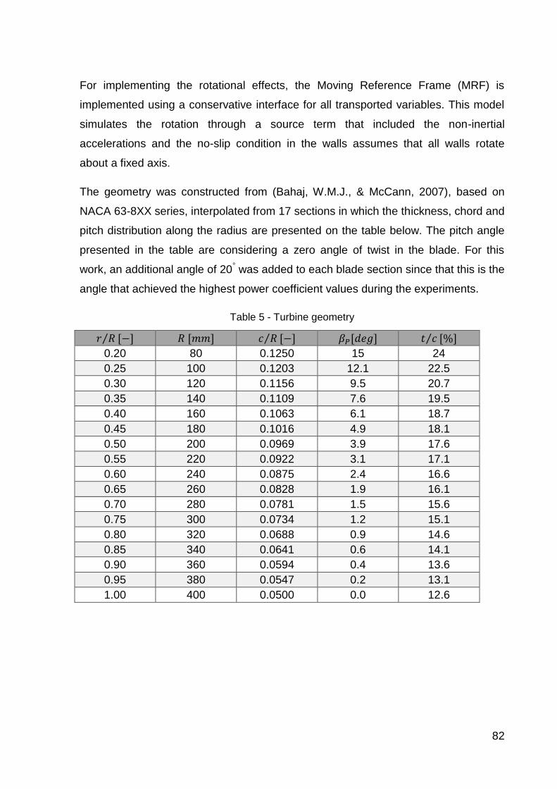
82
For implementing the rotational effects, the Moving Reference Frame (MRF) is
implemented using a conservative interface for all transported variables. This model
simulates the rotation through a source term that included the non-inertial
accelerations and the no-slip condition in the walls assumes that all walls rotate
about a fixed axis.
The geometry was constructed from (Bahaj, W.M.J., & McCann, 2007), based on
NACA 63-8XX series, interpolated from 17 sections in which the thickness, chord and
pitch distribution along the radius are presented on the table below. The pitch angle
presented in the table are considering a zero angle of twist in the blade. For this
work, an additional angle of 20° was added to each blade section since that this is the
angle that achieved the highest power coefficient values during the experiments.
Table 5 - Turbine geometry
𝑟 𝑅⁄ [−] 𝑅 [𝑚𝑚] 𝑐 𝑅⁄ [−] 𝛽𝑃[𝑑𝑒𝑔] 𝑡 𝑐⁄ [%]
0.20 80 0.1250 15 24
0.25 100 0.1203 12.1 22.5
0.30 120 0.1156 9.5 20.7
0.35 140 0.1109 7.6 19.5
0.40 160 0.1063 6.1 18.7
0.45 180 0.1016 4.9 18.1
0.50 200 0.0969 3.9 17.6
0.55 220 0.0922 3.1 17.1
0.60 240 0.0875 2.4 16.6
0.65 260 0.0828 1.9 16.1
0.70 280 0.0781 1.5 15.6
0.75 300 0.0734 1.2 15.1
0.80 320 0.0688 0.9 14.6
0.85 340 0.0641 0.6 14.1
0.90 360 0.0594 0.4 13.6
0.95 380 0.0547 0.2 13.1
1.00 400 0.0500 0.0 12.6

83
7.1.1 Rotating Domain Mesh
Figure 32 - Rotating domain mesh
The Figure 32 shows a general overview of the mesh used in the rotating domain.
For upstream and downstream hubs, a hexahedral unstructured mesh was used. The
turbine disk region was divided into two parts: One close to the blades, that is shown
in Figure 33, in which a hexahedral unstructured mesh was used and other between
two blades in which a structured mesh was used. This division was made to reduce
the number of elements and guarantee a sufficiently refined mesh near to the blades,
even that the turbulence model uses wall functions for the treatment near to the wall.
For mesh validation, the power and thrust coefficients were used since they are the
studied parameters even that additional refinement is necessary to achieve a more
accurate pressure distribution in the blades. However, for performance computation
purposes, a coarser mesh in the blade region with a wall treatment is sufficient
regarding the computational time and hardware limitations.
In the Attachment C, the wall functions are detailed and the ANSYS meshing
recommendations are reviewed. For reasonable results, using the wall functions, it is
needed a minimum of 10 elements inside the boundary layer, which is achieved even
for the blade pitch, with highest flow velocities.

84
Figure 33 - Mesh details in turbine blade region
In all the simulations, an Intel® i7 4510U processor with 2 cores and 4 threads was
used but with the parallel processing limited to 3 threads. This processor has a
nominal clock of 2.00 GHz and can be boosted to 3.1 GHz. The RAM memory is
limited to 16 GB, but since that all other activities consume part of the RAM, the
solver uses about 9 GB for solving the CFD problem in the chosen mesh. It is
possible to uses an additional memory from the HD. However, this process slows
down the processing time.
The Table 6 shows the summary of the simulations performed for the mesh
validation. The convergence was considered achieved when pressure and velocity
residuals were all above 10-5. The y+ was considered as the mean value in the blade.

85
Table 6 - CFD Mesh Validation - Open Flow - TSR = 6 , Re = 1.3 x 10⁶
Blade Wall Sizing [mm]
Domain Sizing [mm]
Power Coefficient
[-]
Thrust Coefficient [-]
y+
[-] Comp.
Time [h]
Number of Elements
[-]
0.50 20 0.321 0.852 149 13 5.2 x 10⁶
0.50 10 0.339 0.861 152 15 5.5 x 10⁶
0.25 6 0.405 0.883 73 52 9.2 x 10⁶
0.40 6 0.391 0.874 121 23 7.2 x 10⁶
0.50 6 0.345 0.871 156 16 5.7 x 10⁶
Figure 34 - y+ used in the turbine - TSR = 6.0

86
7.1.2 Subdomains and Domain Interfaces
The domain has been divided into subdomains to simplify meshing process and
analyzing the rotational effects of the turbine. The subdomains are:
Rotating Domain: Includes the turbine blades and hub. In this domain, it is
applied rotation, therefore are applied a source term for Centrifugal and
Coriolis body forces and the walls included in this domain, in this case, blades
and hub, becomes movable according to a rigid body motion law.
Undeformable Static Domain: Include the fluid domain excluding the rotational
parts for the open domain and confined domain, and excluding the region
close to free surface. The mesh of this domain does not present deformation.
Deformable Static Domain: Includes the region close to the free surface for
open channel analysis. The mesh from this domain is deformable.
The Figure 35 illustrates the rotating domain. The interfaces between the rotating
domain and static domain are defined as a general connection, with a Frozen Rotor
as frame change model, without offset. The program respects the conservation
equations of all variables and the mesh connection is defined as General Grid
Interface (GGI). All other interfaces between subdomains and parts from
subdomains, even in the rotational domain and deformable static domain, are defined
as general connection without frame change model.
Figure 35 - Rotating Domain used in all simulations

87
General Boundary Conditions
For taken into account the effects for considering a non-inertial referential, sources
are added to the rotating domain. This source is calculated by:
𝑆𝑀,𝑟𝑜𝑡 = −𝜌[2(Ω𝑗𝑈𝑘)𝜖𝑗𝑘𝑖 + (Ω𝑗 . 𝑟𝑗)Ω𝑖 − (Ω𝑗 . Ω𝑗)𝑟𝑖] ( 7.1 )
The term 2(Ω𝑗𝑈𝑘)𝜖𝑗𝑘𝑖 corresponds to the Coriolli’s acceleration and the (Ω𝑗 . 𝑟𝑗)Ω𝑖 −
(Ω𝑗 . Ω𝑗)𝑟𝑖 corresponds to the centrifugal acceleration.
The walls, shown in Figure 36, rotates along the turbine axis. The boundary condition
implemented in these regions is that the water velocity is equal to the surface velocity
since the blades and hub are defined as no-slip walls.
The inlet is a velocity inlet with 5% of turbulence intensity. This value is the standard
of Ansys CFX ®, and according to (Blackmore et al., 2014) the turbulence inlet
intensity affects the wake profile and recovery substantially but has a small influence
in the turbine power and thrust. The outlet is defined as a pressure outlet, with a
pressure specified as zero for the open domain and confined domain and determined
iteratively for the open channel domain since the inlet pressure must be equal to the
solid pre-stress. While the other domain boundaries are defined as slip-free walls to
not produce a head loss and do not affect the inlet and outlet velocity profiles since
this analysis is not performed in this work.
The upstream and downstream lengths defined for this work are respectively 10D
and 40 D (8000 mm and 32000 mm), values used on references.
Figure 36 - Rotating Walls

88
7.2 Open Domain
The open domain is schematized on the Figure 37. The static domain is constituted
by blocks to provide a higher refinement in the wake region maintaining the mesh
regularity.
The inlet boundary condition consists in a constant velocity condition with the axial
component with 1.73 m/s and 5% of turbulence intensity (default from Ansys). The
outlet was defined as a pressure outlet with 0 Pa of relative pressure. In the external
diameter of the domain, the pressure is defined as 0 Pa, which is reasonable
regarding to the conditions used to calculate the Betz Limit. The pressure drop is
negligible if the pressure drop energy is compared with the total amount of kinetic
energy available in the inlet flow.
The domain dimensions were adjusted to make the results independent of the
domain size. For upstream length (LU), 10D was used, totalizing 8m and for
downstream length (LD), 40D was used, totalizing 32m. The total length of the
domain is 40 m. For the refined part of the domain, it was defined 0.5D in upstream
and 1.5 D in downstream, with a mesh sizing of 20 mm. For the whole domain, a
mesh size of 100 mm was used. The mesh convergence test indicates that the
results dependency on the mesh sizing on the domain is negligible if compared with
the dependency on the turbine disk region.
The external diameter of the domain is equal to 10000 mm providing a blockage
equal to 0.64% that according to (Garret & Cummins, 2007) increases the power
coefficient in 0.93%, which is negligible if compared with the difference between
numerical and experimental results.
Figure 37 - Open Domain Schematic Drawing

89
7.3 Confined Domain
Both confined domain and open channel domain uses the same 3D model for the
analysis. The domain is divided into three regions:
Rotating Domain
Static Domain
Deformable Domain
The deformable domain is defined as rigid for this case since no mesh deformations
are required. The inlet boundary condition is the same as used for open domain, with
constant velocity with an axial component of 1.73 m/s and 5% of turbulence intensity.
The outlet is defined as a constant pressure outlet, with 11700 Pa, according to the
Table 2. The program calculates the inlet pressure automatically with these boundary
conditions. All walls are modeled as slip-free walls since, in this work, the influence of
profiled flow and channel boundary layer are not considered. The domain upstream
and downstream lengths are the same as used in the open flow model. The
dimensions of the channel are 2.4 m of width by 1.2 m of height, providing a
blockage factor of 17.4%, in which is expected a power increase of 45%, according
to (Garret & Cummins, 2007).
7.4 Open Channel Model – Elastic Free Surface
The two main differences between this model and the confined domain model are
concerning the deformable domain and the free surface region. The deformable part
of the domain, defined as the upper 100 mm of height have mesh deformation based
on displacement diffusion, in which the mesh is updated about the previous mesh,
that for a mesh with all elements with the same size becomes (ANSYS Inc., 2016, p.
Section 1.1.2)
∇2𝛿 = 0 ( 7.2 )
The free surface is coupled with the orthotropic solid by the ANSYS Workbench ®
Coupling, The pressure field in the free surface is transported to the solid, then the
program solves the solid model for obtaining the free surface deformation to update
the fluid model again. The solid model height is 3.6 m, providing an elasticity
modulus of 35100 Pa for obtaining a transversal stiffness of 9778.2 N/m³. The solid is
pre-stressed with 11700 Pa.

90
Chapter 8. Results
In this section, are shown the primary results of the three CFD models and the
comparison between their results. The open domain flow is used mainly for validation
since the experimental data has a blockage correction for guarantee the
independence between the results and the boundary conditions. The confined flow
and the free surface flow results are presented in order to analyze the influence of
the boundary conditions in the turbine hydrodynamic performance.
8.1 Open Domain
For open domain flow, it is shown that the turbine has a low influence in the far flow.
The velocity distribution, shown in the Figure 38, indicates a high-velocity deficit in
the wake region, in a distance below of 2 diameters in the downstream direction. A
small velocity increasing is presented in the bypass region. This increase occurs due
to the flow change of direction due to the presence of the turbine disk. The
streamlines, shown in Figure 39, are not affected in higher domain diameters,
presenting no velocity gradients and no change of direction.
The velocity quickly drops in the wake region, and for fulfilling the mass conservation,
the cross-section in this region has a higher diameter than the turbine disk, as
predicted by the actuator disk theory.
Figure 38 - Velocities on Symmetry Plane for TSR = 6

91
Figure 39 - Typical streamlines for open domain flow
In Figure 40 the streamlines through the turbine disk are compared for different
TSR’s. For the lower TSR, it is clearly shown the turbine has low influence in the
outer flow. The velocity quickly recovers in the wake and the inlet and outlet areas
are almost the same. For higher TSR values, the wake is presented a velocity deficit.
Near to the peak CP, found for TSR = 5.625, the wake has a higher length if
compared with TSR = 8. More power is taken from the flow requiring a higher length
for the recovery. The higher TSR presents a shorter wake length with the highest
section area, which is expected since for a higher rotation is expected that the turbine
affects the flow in the same way as a disk.

92
Figure 40 - Streamlines through turbine disk for Open Flow
TSR = 2.0
TSR = 5.0
TSR = 5.5
TSR = 6.0
TSR = 8.0

93
The comparison between the figures above shows the difference between the
pressure distributions in the blades for different TSR’s. It is seen that for the TSR =
6.0, the pressure on the suction side is lower than the calculated for TSR = 5 and
TSR = 5.5. It occurs due to the higher absolute speed of each blade section. Even
with lower effective attack angles, this increase in the speed leads to higher pressure
drops.
Figure 41 - Pressure on Blades for TSR = 5.0
Figure 42 - Pressure on Blades for TSR = 5.5
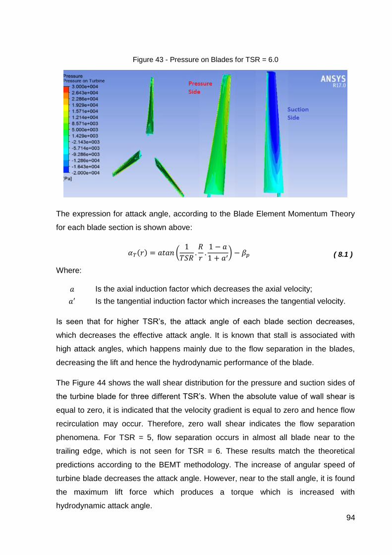
94
Figure 43 - Pressure on Blades for TSR = 6.0
The expression for attack angle, according to the Blade Element Momentum Theory
for each blade section is shown above:
𝛼𝑇(𝑟) = 𝑎𝑡𝑎𝑛 (1
𝑇𝑆𝑅.𝑅
𝑟.
1 − 𝑎
1 + 𝑎′) − 𝛽𝑝 ( 8.1 )
Where:
𝑎 Is the axial induction factor which decreases the axial velocity;
𝑎′ Is the tangential induction factor which increases the tangential velocity.
Is seen that for higher TSR’s, the attack angle of each blade section decreases,
which decreases the effective attack angle. It is known that stall is associated with
high attack angles, which happens mainly due to the flow separation in the blades,
decreasing the lift and hence the hydrodynamic performance of the blade.
The Figure 44 shows the wall shear distribution for the pressure and suction sides of
the turbine blade for three different TSR’s. When the absolute value of wall shear is
equal to zero, it is indicated that the velocity gradient is equal to zero and hence flow
recirculation may occur. Therefore, zero wall shear indicates the flow separation
phenomena. For TSR = 5, flow separation occurs in almost all blade near to the
trailing edge, which is not seen for TSR = 6. These results match the theoretical
predictions according to the BEMT methodology. The increase of angular speed of
turbine blade decreases the attack angle. However, near to the stall angle, it is found
the maximum lift force which produces a torque which is increased with
hydrodynamic attack angle.

95
Figure 44 - Shear stress on blades
The figures above show the comparison between the experimental results and the
CFD results. The power coefficient is underpredicted if compared with the
experiments and the thrust coefficient is overpredicted. The increase of CT with the
turbine rotation is in which the turbine is closer than a disk, which causes a higher
restriction to the flow than a turbine with a lower rotation.
In (Afgan et al., 2012), in which both turbulence models were compared, the CFD
results were closer to the experimental analysis for LES, however, analyzing the
performance through the same model used in this work, the underprediction is almost
the same.
Accordingly, both power and thrust evaluations showed the same trend by
experimental methodology and by CFD approach. Therefore, the CFD model used in
this work is validated for a first analysis of the tidal current turbine, being useful for a
more accurate design of the blade if compared with BEMT. However, for the final
geometry, a more robust CFD approach and an experimental analysis still required.

96
Figure 45 - Comparison between Experimental and CFD Results: Thrust Coefficient
Figure 46 - Comparison between Experimental and CFD Results: Power Coefficient
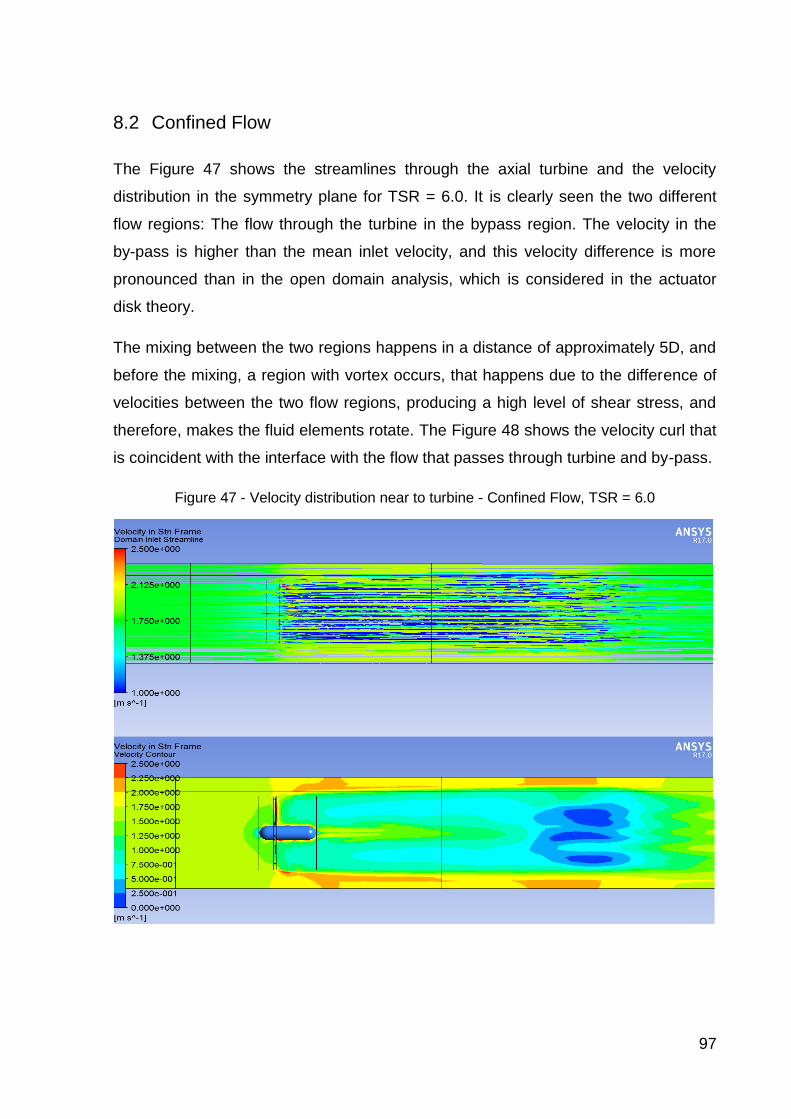
97
8.2 Confined Flow
The Figure 47 shows the streamlines through the axial turbine and the velocity
distribution in the symmetry plane for TSR = 6.0. It is clearly seen the two different
flow regions: The flow through the turbine in the bypass region. The velocity in the
by-pass is higher than the mean inlet velocity, and this velocity difference is more
pronounced than in the open domain analysis, which is considered in the actuator
disk theory.
The mixing between the two regions happens in a distance of approximately 5D, and
before the mixing, a region with vortex occurs, that happens due to the difference of
velocities between the two flow regions, producing a high level of shear stress, and
therefore, makes the fluid elements rotate. The Figure 48 shows the velocity curl that
is coincident with the interface with the flow that passes through turbine and by-pass.
Figure 47 - Velocity distribution near to turbine - Confined Flow, TSR = 6.0

98
Figure 48 - Velocity Curl for Confined Flow - TSR = 6
In Figure 49, the differences in the wake between confined domain and open domain
are analyzed. The first difference is concerning the wake length. The confined
domain has a wake length at least 2.5 times higher than the analyzed for the open
domain. The flow confinement transports the vorticity of the wake flow becoming
more difficult the dissipation of the flow rotation. This effect is expected since higher
turbulence levels decrease the wake length. For confined flows, the by-pass flow has
lower inertia if compared with open domain by-pass, which makes the wake more
stable. A result of this analysis is that for channel flows with high blockage ratio, even
the individual performance of each turbine is expected to increase, and the turbines
must be placed within a greater axial distance that could result in a decrease of the
total power generated in the farm.
The wake width is lower for the confined domain. It is expected since the
confinement restricts the wake expansion.
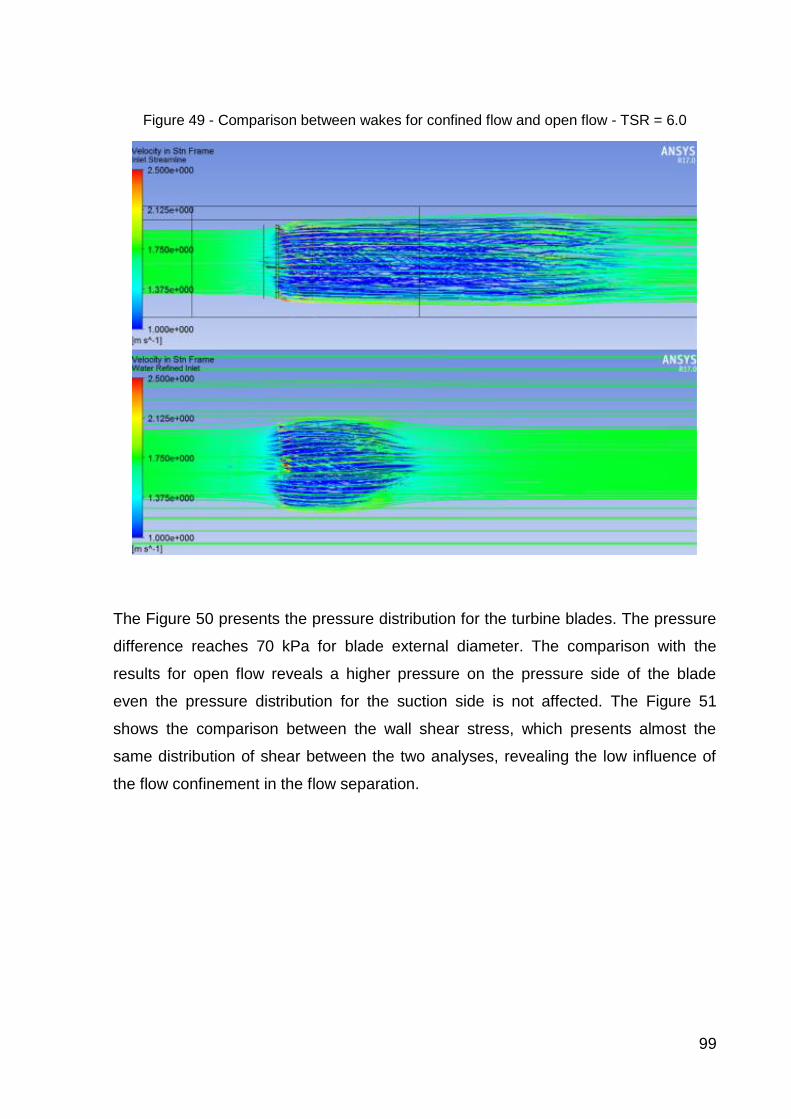
99
Figure 49 - Comparison between wakes for confined flow and open flow - TSR = 6.0
The Figure 50 presents the pressure distribution for the turbine blades. The pressure
difference reaches 70 kPa for blade external diameter. The comparison with the
results for open flow reveals a higher pressure on the pressure side of the blade
even the pressure distribution for the suction side is not affected. The Figure 51
shows the comparison between the wall shear stress, which presents almost the
same distribution of shear between the two analyses, revealing the low influence of
the flow confinement in the flow separation.

100
Figure 50 - Pressure distribution on blades for confined flow
Figure 51 - Comparison between confined domain and open domain - Wall Shear Stress

101
8.3 Open Channel
The open channel flow is modeled with an elastic wall approach. However, for the
velocity of 1.73 m/s, the pressure difference between upstream and downstream
regions together with the blockage ratio in order of 20% led to a free surface
instability. The streamlines for the model for TSR = 6.0 are shown in the Figure 53, it
is seen the interference between the turbine wake and the free surface, in which
regions with high speed occurs. There flow vorticity is clear near to the free surface.
This interaction made the model diverges after 7 Fluid-Structure coupling iterations
due to negative Jacobian elements formed due to the high deformation of the free
surface in the downstream region. This problem did not occur in (Mattavo & Assi,
2017) in which the distance between the obstacle and the free surface is higher than
the obstacle diameter.
For analysis of the dimensionless power and thrust coefficients, the simulation was
carried out with an inlet velocity of 10% than the original model, with the rotation
decreasing to maintain the same TSR values. This new model resulted in a Reynolds
Number of 1.5 x 10⁵. This adjustment is expected to reduce the pressure drop to 1%
of original value and according to the equation (C.26) and the same decreasing is
expected for the head difference between the inlet and outlet.
In (Mason-Jones et al., 2012) the authors concluded that for a Re > 3 x 10⁵ the
power and thrust coefficients are a function only of TSR, however, since the analyses
were conducted without free surface effects, this value could not be used as a
reference. However, considering the preliminary stage of development of the elastic
free surface methodology, the analysis with this inlet velocity is valid for testing the
model capabilities.
The model with inlet velocity of 1.73 m/s, shown in Figure 52, presented for a TSR
equals to 6.0 a CP of 0.29 and CT of 0.79 while the model with the inlet velocity of
0.173 m/s shown in Figure 53, presented for the same TSR value a CP of 0.393 and
CT of 0.83.
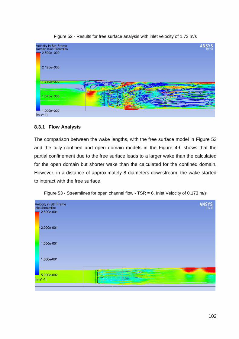
102
Figure 52 - Results for free surface analysis with inlet velocity of 1.73 m/s
8.3.1 Flow Analysis
The comparison between the wake lengths, with the free surface model in Figure 53
and the fully confined and open domain models in the Figure 49, shows that the
partial confinement due to the free surface leads to a larger wake than the calculated
for the open domain but shorter wake than the calculated for the confined domain.
However, in a distance of approximately 8 diameters downstream, the wake started
to interact with the free surface.
Figure 53 - Streamlines for open channel flow - TSR = 6, Inlet Velocity of 0.173 m/s

103
Figure 54 –Detail of Turbine Wake (Left) and Detail of Free Surface Instabilities (Right)
The Figure 55 presents the streamlines for the entire fluid domain. There is an
increase in velocity in the turbine by-pass, colored in yellow.
Looking to the downstream part of the domain, far from the free surface, the velocity
returns to the inlet velocity, which is expected considering negligible deformations of
the free surface. However, in Figure 54, in the detail of free surface instabilities, is
presented an increase of about 50% in the mean speed in the free surface region.
The Figure 58 presents the contour of velocity curl in the fluid domain. According to
the Figure 56 This curl intensity is similar to the induced by the tip blades. The Figure
57 presents the velocity curl isosurfaces in the fluid domain. An interaction between
the tip vortex and the vorticity in the free surface seems to happen. However, is
essential to highlight that it is not known at the present moment if such effect would
happen in a real flow or if it is caused just by numerical instabilities.
Figure 55 – Streamlines for Open Channel Flow – TSR = 6 – Inlet Velocity of 0.173 m/s – View of the entire domain

104
Figure 56 - Velocity Curl Contour- for Open Channel Flow – TSR = 6 – Inlet Velocity of 0.173 m/s
Figure 57 - Velocity Curl Isosurface- for Open Channel Flow – TSR = 6 – Inlet Velocity of 0.173 m/s

105
The vortices in the wake region are also seen in the Figure 58. The differences
between the velocities in this region, with higher speed above and below turbine disk
together with velocities 30% higher near to the turbine axis induces shear stress in
the flow that makes the fluid particles rotate, starting the vertical formation. The wake
is not symmetrical concerning the turbine center horizontal plane. It may occur due to
the free surface, and it is also seen by the velocity curl contour, velocity curl
isosurfaces and the streamlines.
The Figure 59 shows a uniform velocity profile with exception to the interface region
between the static domain and Indeformable domain.
In the Figure 60the velocity distribution in the turbine disk is presented. High
velocities in the blades suction side and low velocities in the blade pressure side are
seen, which is expected since the main motion load is the lift produced in those
regions that causes a torque that powers the turbine.
The downstream profile of velocity is presented from the Figure 61 to the Figure 64.
The first figure shows the velocity contour for a distance of 1 turbine disk diameter
from the turbine disk plane. It is seen a velocity defect in the turbine disk region,
which is already expected since it represents the wake region. There is an increase
of the velocity close to the free surface above to the turbine disk.
Figure 58 - Velocity Contour - for Open Channel Flow – TSR = 6 – Inlet Velocity of 0.173 m/s

106
Figure 59 - Inlet Velocity Profile – Distance of 1 Diameter from Turbine Disk
Figure 60 – Turbine Disk Velocity Profile
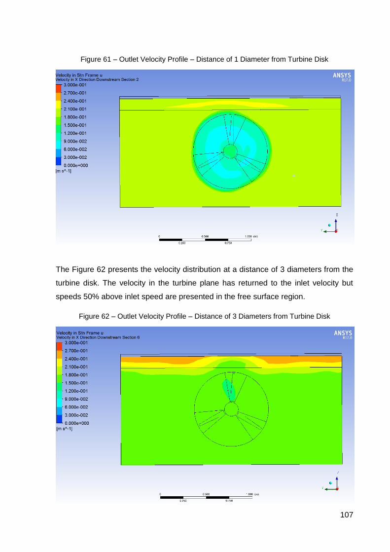
107
Figure 61 – Outlet Velocity Profile – Distance of 1 Diameter from Turbine Disk
The Figure 62 presents the velocity distribution at a distance of 3 diameters from the
turbine disk. The velocity in the turbine plane has returned to the inlet velocity but
speeds 50% above inlet speed are presented in the free surface region.
Figure 62 – Outlet Velocity Profile – Distance of 3 Diameters from Turbine Disk

108
The Figure 63 presents the velocity distribution 6 diameters downstream from the
Turbine Disk. There is a velocity level almost 100% above the inlet velocity. This
region presents a high vorticity as discussed previously. The Figure 64 presents the
velocity profile 10 diameters from the turbine disk. The velocity on the free surface
region decreased but still 50% above the inlet velocity.
Figure 63 – Outlet Velocity Profile – Distance of 6 Diameters from Turbine Disk
Figure 64 – Outlet Velocity Profile – Distance of 10 Diameters from Turbine Disk

109
8.3.2 Deformations in the Solid Model
Figure 65 - Stresses in Z-Direction – TSR = 6 ; Inlet velocity of 0.173 m/s
Figure 66 - Orthotropic Body deformation - TSR = 6; Inlet Velocity of 0.173 m/s
The Figure 65 shows the stresses in z-direction distribution and the Figure 66 shows
the deformations in the free surface region. As expected, the negative deformations
correspond to positive stresses on the body (traction), and the positive deformations
correspond to negative stresses on the body (compression), which shows that the
body assumes the spring behavior, necessary to this free surface modelling.
110
An issue regarding to this model is related to the solid pre-stress. Since in the
boundary conditions, the only specified pressure is the outlet, and the model initially
assumes that the inlet deformation is zero, the definition of the solid pre-stress must
make the inlet pressure equals to the solid pre-stress which is not directly defined in
this model. Hence, for the model consistency, the outlet pressure was adjusted to the
inlet pressure achieve the same pressure as the calculated for the pre-stress.
However, for the subsequent coupling interactions between the solid and fluid
models, the pressure difference between inlet and outlet changes, requiring an
additional updated in the outlet pressure, which is not possible only using the ANSYS
Workbench 17.0 ®. It caused an inlet deformation, shown in Figure 65. However,
since the distance between the inlet and the turbine disk is 8000 mm and the
deformation order is 25 mm, the flow had become uniform before passing through
the turbine.
None the less, for further simulations, a code must be implemented within the
ANSYS CFX to make the outlet pressure iterative to guarantee the zero deformation
at the flow inlet.

111
8.4 Comparison Between the CFD Models
As expected, the confined domain presented the higher power coefficient, by
comparison with the open domain and open channel domain. The confinement
guarantees that a higher portion of fluid passes through the turbine disk, and thus, a
higher kinetic energy flow passes through the turbine disk too.
The calculated power coefficient for the confined flow was 11.5% higher than the
calculated for open domain flow. The prediction according to (Garret & Cummins,
2007) of 45% did not confirm, which is expected due to the simplicity of the theory,
which only analyses the flow in one direction, neglecting the geometrical
particularities of the turbine and other flow characteristics.
The open channel model, for the case with 0.173 m/s inlet velocity presented the
same power coefficient of the open domain flow, however, due to the difference of
the Reynolds number between the two simulations, this comparison cannot be
precisely made, since the effects of the Reynolds number are not known for this
case. However, the instabilities in the wake, presented for the open channel model,
indicated that the model did not fully converge. The graphic comparing the power
coefficients in the different boundary conditions is shown in Figure 67.
Figure 67 - Comparison between the power coefficients between the different boundary conditions

112
The data of thrust coefficient, shown in Figure 68, indicates that the confinement
increases the axial thrust of the turbine, which causes higher pressure differences
than the open flow and the open channel cases. The average difference between
open flow and confined domain cases is 8%, lower than the difference found for
power coefficient measurements. It indicates to a higher efficiency of the turbine with
the flow confinement.
For the open channel cases, both simulations led to a lower thrust coefficient, which
is inconsistent with the actuator disk theory. For the simulation with lower inlet
velocity, the result almost matched with the open domain case. However, according
to the actuator disk theory, the increase of Froude number causes an increase in the
power coefficient, that is shown in Figure 69.
Figure 68 - Comparison between the thrust coefficients between the different boundary conditions
Figure 69 - Power coefficient in function of Froude Number according to the actuator disk theory for an open channel

113
Chapter 9. Conclusion
The comparison of the CP and CT curves between experimental methodology and
computational results for the open domain geometry showed that the CFD has a
good agreement with the experiments, validating the computational method and its
features, such as the mesh density and turbulence models used. The curves
obtained through CFD presented the same shape of the curves obtained through
experiments, however, underpredicted the generated power and overpredicted the
thrust, which is already expected according to the literature.
The analysis with the confined domain showed that the blockage increases the
generated power which agrees with the theoretical predictions. The wake length is
higher, which could decrease a tidal farm total generation since the mean velocity in
the wake region is lower than the inlet velocity. A computational analysis varying the
blockage ratio is missing to evaluate the impact of this variable on the hydrodynamic
performance of an axial tidal current turbine.
The confinement has a low influence in the flow separation pattern, which is
highlighted by the comparison between the wall shear stress plots. Additional
investigations must be performed to analyze the influence of the boundaries in the
flow through the blades which increases the generated power. With the current
simulations, any statement could be made regarding to the attack angles and the
difference between this parameter comparing the different boundary conditions used
in this work.
Regarding the free surface model using an elastic free surface, the results for the
original Reynolds and Froude number was not accurate and did not converge, due to
the high initial deformation presented, nevertheless, the thrust calculation showed
missprediction about 16% if compared with the confined domain.
The non-convergence of the elastic free surface for the initial inlet velocity occurred
due to the high initial deformations, compared with the cross-sectional area. These
deformations induced high-velocity gradients in the free surface region which caused
high pressures, making the algorithm became unstable. Further development on this
114
algorithm shall include a gradual deformation of the free surface in order to avoid
such problems.
For the free surface methodology analysis, the simulation with 10% of inlet velocity
was performed providing a good approach for both torque and thrust, and
considering that the Froude number was decreased with the inlet velocity, it is
expected that the simulation for the original Froude number would provide a higher
power and thrust values.
The analytical models, analyzed in section 6.1, showed that the proposed model is
physically consistent, providing the same balance between potential and kinetic
energy as the gravity-based models, as the VOF methodology. Moreover, the CFD
analysis with the elastic free surface model provided feasible results, which
contributes to validate the potential of the methodology to analyze free surface flows.

115
Chapter 10. Proposals for complementary works
Even this work is focused on the hydrodynamic analysis of tidal current turbines, the
methodology implemented for free surface analysis has shown to be promising since
it is computationally efficient if compared with VOF approach and presents fewer
problems related to numerical diffusion in the free surface region. Therefore, the
complementary works cover both areas.
10.1 Tidal current turbines
This work evaluated a single turbine subjected to different boundary conditions. All
performed analysis was made in a steady state condition. Therefore, analyses
involving transient analyses such as the pressure fluctuations due to rotational
effects are necessary to evaluate the order of the power fluctuations in power
generated. The simulation of symmetry and anti-symmetry conditions is not found in
the literature.
The more recent experimental analysis evaluated the interaction between two
turbines placed on the same axis. A numerical analysis of such problem is interesting
to evaluate the interaction mechanisms and assessing parameters as the difference
of rotation between the two turbines and the rotation inversion in the total generated
power.
Several analyses of tidal farm generation optimization are found in the literature,
indicating that most of the researches see more benefits in optimizing the whole farm
than a single turbine. However, most CFD optimization techniques assume a
constant CT and CP for all turbines, neglecting the influence of inlet velocity on such
parameters.

116
Therefore, the following works are suggested for the theme development continuity:
Transient analysis of tidal current turbine confined in a closed channel with
high blockage and transient analysis of tidal current turbine in an open
channel;
Transient BEMT method involving the interaction between the blade and the
free surface;
Steady State and Transient analysis of two tidal current turbines placed on the
same axis;
Optimization analysis of a tidal current farm using CP and CT calibrated with a
real turbine experimental and numerical analysis.
10.2 Free surface analysis
The elastic free surface used during this work produced accurate results for the tidal
current turbine analysis, and the analytical development showed the physical
consistency of such methodology that provides energy conservation and even for
transient analysis, could have its density adjusted to produce feasible results.
However, since in the current bibliography, it was not found any similar methodology,
it is needed a more profound analysis.
Furthermore, only parameters such as thrust and torque were evaluated during the
CFD analysis. Hence, it is needed analysis comparing the flow pattern and the
velocity profiles with the measured experimentally and with the obtained through
VOF methodology with the free surface.
Besides of that, during the process of Fluid-Structure coupling, it issues with
convergence, mainly due to the mesh deformation algorithm were found. The
standard method from ANSYS CFX® is based on displacement diffusion, and for
domains with small volumes, this could cause negative volumes, being physically
and computationally infeasible, stopping the calculation routine.

117
Since more validation cases, theoretical development and a consistent computational
implementation still needed, it is proposed the following works:
Evaluate the impacts of this boundary condition in a viscous fluid flow
analytically;
Analyse the velocity profiles for flow around a circular cylinder with steady-
state and transient analysis;
Analyse the flow through a circular cylinder piercewising the free-surface;
Couple the elastic free surface methodology with a more robust mesh
deformation algorithm, designed for large deformations. An elastic mesh is
proposed in (Battaglia et al., 2004) for solving a free surface problem, showing
a trend of the solution of such problem.
The study of solution stability of this methodology.

118
Chapter 11. References
Afgan et al. (2012). Large-Eddy Simulation of a 3-bladed horizontal axis tidal stream
turbine: comparisons to RANS and experiments. Turbulence, Heat and MAss
Transfer(7), 1 - 13.
Andritz Hydro. (s.d.). Hydro News 27 - Tidal Energy. Acesso em 04 de January de
2018, disponível em https://www.andritz.com/hydro-en/hydronews/27/hy-
news-27-03-tidal-energy-hydro
ANSYS Inc. (2016). Ansys 17.0 Users Guide . ANSYS Inc.
Bahaj, A., W.M.J., B., & McCann, G. (2007). Experimental verifications of numerical
predictions for the hydrodynamic performance of horizontal axis marine
current turbines. Renewable Energy, 2479-2490.
Barnsley M.J., W. J. (1990). Final report on 2nd phase of development and testing of
a horizontal axis wind turbine test rig for the investigation of stall regulation
aerodyamics. Carried out under ETSU Agreement E.5a/CON5103/1746 .
Battaglia et al. (2004). Numerical Simulation of Transient Free Surface Flows Using a
Moving Mesh Technique. ENIEF.
Betz, A. (1920). Das Maximum der theoretisch möglichen Ausnützung des Windes
durch Windmotoren. Zeitschrift für das gesamte Turbinenwesen.
Bir et al. (2011). Structural Design of a Horizontal-Axis Tidal Current Turbine. ASME
30th International Conference on Oceanic Offshore and Artic Engineering.
Roterdam.
Biskup et al. (2014). mulation of Fluid-Structure Interaction on Tidl Current Turbines
Based on Coupled Multibody and CFD Methods. Journal of Ocean and Wind
Energy, 1(2), 119 - 126.
Blackmore et al. (2014). Influence of turbulence on the wake of a marine current
turbine simulator. Southampton: Royal Society Publishing.

119
British Hydro. (14 de October de 2009). Fonte: British Hydro Org: http://www.british-
hydro.org/downloads/La%20Rance-BHA-Oct%202009.pdf
Consul, C. (2011). Cross Flow Turbine. In: Hydrodynamic Analysis of a Tidal Cross-
Flow Turbine. Trinity: Worscester College.
Empresa de Pesquisas Energéticas. (12 de November de 2017A). Leilão de Energia
A4-2017. Fonte: Empresa de Pesquisas Energéticas:
http://www.epe.gov.br/leiloes/Documents/Resumo%20Cadastramento%20-
%20Leil%C3%A3o%20A-4%202017%20(v3).pdf
Empresa de Pesquisas Energéticas. (12 de November de 2017B). Leilão de Energia
A6/2017. Fonte: Empresa de Pesquisas Energéticas:
http://www.epe.gov.br/leiloes/Documents/Resumo%20Cadastramento%20-
%20Leil%C3%A3o%20A6%202017%20(v3).pdf
Estafahani, J., & Karbasian, H. (2012). Optimizing the Shape of Rotor Blades for
Maximum Power Extraction in Marine Current Turbines. International Journal
of Automotive and Mechanical Engineering, 6, 722-729.
Falnes, J. (2007). A Review of wave-energy extraction. Marine Structures 20.
Ferziger, J., & Peric, M. (2002). Free-Surface Flows. In: Computational Methods for
Fluid Dynamics (pp. 381 - 397). Springer.
Forinash, C., & DuPont, B. (2016). Optimization of floating offshore wind energy
systems using an extended pattern search method. Proceedings of the ASME
2016 35th International Conference on Ocean, Offshore and Artic
Engineering. Busan.
Galloway et al. (2011). Experimental and numerical results of rotor power and thrust
of tidal turbine operating at yaw and in waves. World Renewable Energy
Congress 2011. Linköping.
Garret, C., & Cummins, P. (2007). The efficiency of a turbine in a tidal channel.
Journal of Fluid Mechanics, 588, 243 - 251.

120
Gebreslassie et al. (2012). Comparison of Analytical and CFD Modelling of the Wake
Interactions of Tidal Turbines. Exeter: College of Engineering, Mathematics
and Physical Sciences from University of Exeter.
Gelfand, I., & Fomin, S. (1963). The General Variation of a Functional. In: Calculus of
Variations (pp. 54 - 66). Prentice Hall.
Green Rhyno Energy. (16 de May de 2018). Wind Energy and the Environment.
Fonte: Green Rhyno Energy:
http://www.greenrhinoenergy.com/renewable/wind/wind_environment.php
Hansen, J. (2015). Ice melt, sea level rise and superstorms. Atmospheric, Chemistry
and Physics Discussions, p. 20062.
Houlsby et al. (2007). Application of Linear Momentum Actuator Disc Theory to Open
Channel Flow. Oxford: University of Oxford - Department of Engineering
Science.
Hughes, T. (2000). Fundamental Concepts - A Simple one-dimensional boundary-
value Problem. In: The Finite Element Method - Linear Static and Dynamic
Finite Element Analysis (pp. 1 - 56). New York: Dover Publications Inc.
International Energy Agency. (2017). Global Electrical Vehicules Outlook 2017.
International Energy Agency.
IRENA. (2014). IRENA Ocean Energy Technology Brief 3.
Jones, W., & Launder, B. (1972). The prediction of laminarization with a two-equation
model of turbulent. Journal of Heat and Mass Transfer 15, 301-314.
K Water. (s.d.). K Water. Acesso em 18 de December de 2017, disponível em
http://english.kwater.or.kr/eng/busi/project03Page.do?s_mid=1192
Kim, J., & Moser, R. (1987). Turbulence statistics in fully developed channel flow at
low Reynolds Number. Journal of Fluid Mechanics 177, 133-166.
Kulkarni et. al. (2016). Computational Fluid Dynamic (CFD) Mesh Independency
Study of a Straight Blade Horizontal Axis Tidal Turbine. Birmingham:
Birmingham City University.

121
Lai, M., Krempl, E., & Ruben, D. (2010). Linearly Elastic Solid. In: Introduction to
Continuum Mechanics (pp. 204 - 207). Elsevier.
Lamb, H. (1879B). Waves due to a Submerged Cylinder. In: Hydrodynamics (pp. 410
- 413). Cambridge University Press.
Lanczos, C. (1949). Mechanics of the Continua. In: The variational principles of
mechanics (pp. 365 - 369). University of Toronto Press.
Launder, B., & Spalding, D. (1974). The numerical computation of turbulent flows.
Computational Methods Applied to Mechanical Engineering, 269-289.
Lloyd et al. (2011). Unsteady CFD of a Marine Current Turbine using OpenFOAM
with Generalized Grid Interface. University of Southampton.
Maliska, C. (2014). Transferência de Calor e Mecânica dos Fluidos Computacional -
2ed. Rio de Janeiro: LTC.
Mason-Jones et al. (2012). Non-dimensional scalling of tidal stream turbines. Energy,
444, 820 - 829.
Masters et al. (2011). A robust blade element momentum theory for tidal stream
turbines including tip and hub loss corrections. Journal of Marine Engineering
and Technology, 11, 25 - 35.
Masters et al. (2015). A Comparison of Numberical Modelling Technique for Tidal
Stream Turbine Analysis. Energies, 8, 7833-7853.
Mattavo, F., & Assi, G. R. (2017). Free Surface Modeling Employing a Two-Way
Fluid Structure Interaction Approach for the Flow Around a Circular Cylinder.
COBEM 2017. Curitiba.
Meirovitch, L. (2001). Distributed Parameters System: Exact Solutions. In:
Fundamentals of Vibrations (pp. 374 - 464). McGraw Hill.
Menter, F. (1992). Improved Two-Equation k-ω Turbulence Model for Aerodynamic
Flowx. California: NASA.
Ministério de Minas e Energia do Brasil. (2017). Capacidade instalada de geração de
energia no Brasil e no Mundo.

122
Morris et al. (2016). Evaluatio of the swirl characteristics of a tidal stream turbine
wake. International Journal of Marine Energy, 14, 198 - 214.
Munson et. al. (2004). Semelhança, Análise Dimensional e Modelos. In:
Fundamentos da Mecânica dos Fluídos - Tradução da quarta edição
americana (pp. 344 - 397). Edgard Blucher.
Munson, B., Young, D., & Okiishi, T. (2002). Fundamentos da Mecânica dos Fluidos -
Tradução da 4a edição americana. São Paulo: Blucher.
Newman, J. (1977). Marine Hydrodynamics. Massachusetts: MIT Press.
Newman, J. (1977-A). Marine Hydrodynamics. In: J. Newman, Marine
Hydrodynamics (pp. 237 - 327). Massachusetts: MIT Press.
Pantankar, S. (1980). Numerical Heat Transfer and Fluid Flow. Hemisphere
Publishing Corporation.
Peiró et al. (2007). Modelling of free surface proximity and wave induced velocities
around a horizontal axis tidal stream turbine. Proceedings of the 7th European
Wave and Tidal Energy Conference. Porto.
Piggott et al. (2014A). Tidal turbine array optimisation using the adjoint approach.
Renewable Energy, pp. 658 - 673.
Piggott et al. (2014B). A hierarchy of approaches for the otpimal design of tidal
turbine farms. 5th International Conference on Ocean Energy. Halifax.
Pinón et al. (2012). Numberical Simulation of the ake of marine current turbines with
a particle method. Renewable Energy, 46, 111 - 126.
Pinón et al. (2014). Experimental study of the turbulence intensity effects on marine
current turbines behaviour. Part One: Single Turbine. Renewable Energy, 66,
729 - 746.
Pinón et al. (2014B). Experimental study of the turbulence intensity effects on marine
current turbines behaviour. Part II: Two interacting turbines. Renewable
Energy, 68, 876 - 892.

123
Pope, A. (1951B). The Juokowski Transformation. In: A. Pope, Basic Wing and Airfoil
Theory (pp. 76-99). New York: McGraw Hill.
Pope, S. (2000). Turbulent Flows. Cambridge: Cambridge University Press.
Profito, F. (2015). On the Development of Advanced Texhniques for Mixed-
Elastohydrodynamic Lubrification Modelling of Journal and Sliding Bearing
System. São Paulo.
Rao, S. (2008). Sistemas Contínuos. In: Vibrações Mecânica - Quarta Edição (pp.
272 - 304). Pearson Prentice Hall.
Reichl et al. (2005). Flow past a cylinder close to a free surface. Journal of Fluid
Mechanics, 533, 269 - 296.
Rhie, C., & Chow, W. (1982). A numerical study of the turbulent flow past an isolated
airfoil with trailing edge separation. 3rd Joint Thermophysics, Fluids, Plasma
and Heat Transfer Conference. St Louis.
Salter et al. (2002). Power conversion mechanisms for wave energy. Journal
Engineering for the Maritme Environment, Vol 216, 1 - 27.
Salvatore et. al. (8 de May de 2018). Marine Turbine Hydrodynamics by a Boundary
Element Method with Viscous Flow correction. Journal of Marine Science and
Engineering, pp. 1-30.
Sharma et al. (2013). Characteristics of the turbulence in the flow at a tidal stream
power site. Auckland: Royal Society Publishing.
Souza, Z. (2011). Perda de energia por fuga. In: Z. Souza, TOMO IV - Projeto de
Máquinas de Fluxo - Turbinas Hidráulicas com rotores axiais (p. 116). Rio de
Janeiro: Interciência.
Stansby, P., & Stallard, T. (19 de February de 2016). Fast optimisation of tidal stream
turbine positions for power generation in small arrays with low blockage based
on superposition of self-similar far-wake velocity deficit profiles. Renewable
Energy, pp. 366 - 375.

124
Tatum et al. (2016). CFD Modelling of a tidal stream turbine subjected to profile flow
and surface gravity effects. International Journal of Marine Energy(15), 156 -
173.
The Guardian. (17 de July de 2008). First tidal power turbine gets plugged in. Acesso
em 04 de January de 2018, disponível em
https://www.theguardian.com/environment/2008/jul/17/waveandtidalpower.ren
ewableenergy
TidalEnergy Today. (17 de February de 2015). Tidal Energy Today. Acesso em 20
de october de 2017, disponível em
http://tidalenergytoday.com/2015/02/17/estimate-of-global-potential-tidal-
resources/
Timoshenko, S. P., & Goodier, J. (2010). Theory of Elasticity 3rd Edition. In: Theory
of Elasticity 3rd Edition. McGraw Hill.
U.S. Energy Information Administration. (2016). International Energy Outlook 2016.
Washington DC: U.S. Energy Information Administration.
U.S. Energy Information Administration. (2017). Short-Term Energy Outlook -
November 2017.
Uihlein, A., & Magagna, D. (2016). Wave and Tidal current energy - A review of the
current state of researche beyond technology. Renewable and Sustainable
Energy Reviews 58, 1070 - 1081.
UOL Confere. (November de 12 de 2017). Fonte: UOL Confere:
https://noticias.uol.com.br/confere/ultimas-noticias/2017/03/28/uol-confere-
trump-contradiz-estudos-ao-defender-economia-antes-do-clima.htm
Wang, S., Li, Q., Fang, C., & Zhou, C. (2016, January 15). The relationship between
economic growth, energy consumption, and CO2 emissions: Empirical
evidence from China. Science of The Total Environment, Volume 542, pp. 360
- 371.
Wilcox, D. (1994). Turbulence Modeling for CFD. California: DCW Industries.

125
World Energy Council. (2016). World Energy Resources - 2016. London: World
Energy Council.
Zhang et al. (2017). Experimental Analysis and Evaluayion of the Numberical
Prediction of Wake Characteristics of Tidal Stream Turbine. Energies(10).

126
ATTACHMENT A – Potential Fluid Flow
A.1 – Flow through a circular cylinder
Using the definition of complex potential from the equation (5.30) it is possible to
transform two domains by a transformation known as conformal mapping. One can
use a specific transformation called Kutta-Juokowski transformation to transform a
cylindrical domain to a plane domain. The transformation is defined by the equation
below.
휁 = 𝜉 + 𝑖휂 = 𝑧 +𝐶2
𝑧 (A1.1)
Transforming the flow Φ(𝜉) = 𝑈. 𝜉 related to uniform stream to the plane z, according
to the Kutta-Jukowisky transformation, where the constant is equal to the cylinder
radius, the complex potential becomes:
Φ(𝑧) = 𝑈 (𝑧 +𝑅2
𝑧) = 𝑈. 𝑟 [𝑒𝑖𝜃 + (
𝑅
𝑟)
2
𝑒−𝑖𝜃] (A1.2)
Considering only the real part of the potential:
Φ(𝑟, 휃) = 𝑈𝑟 [1 + (𝑅
𝑟)
2
] cos(휃) (A1.3)
Transforming the last equation to Cartesian coordinates:
Φ(𝑥, 𝑦) = 𝑈𝑥 (1 +𝑅2
𝑥2 + 𝑦2) (A1.4)
Figure 70 - Kutta-Juokowski transformation applied to a circular cylinder

127
A.2 – Gravity Waves
The gravity waves for high depths could be analysed using the potential flow theory.
For this Phenom, the seabed viscous effects are negligible and due to the oscillation
scales, the turbulent effects could be unconsidered. Hence, the fluid flow shall
respect the Laplace’s equation.
According to (Newman, Marine Hydrodynamics, 1977-A), the boundary conditions
are:
i. No flux of mass through the free surface 휂(𝑥, 𝑡)
ii. Constant pressure along the free surface
iii. No flux of mass through the seabed 휂(𝑥, 𝑡)
The first boundary condition states that a particle belonging to the free surface must
remain always in the free surface. It means that the velocity of the particle must be
always tangent to the free surface curve. Defining the curve in a 2D space
representing the free surface, 𝛾(𝑥, 𝑡) = [𝑥, 휂(𝑥, 𝑡)]. The velocity vector on the free
surface is given by:
𝑑
𝑑𝑡𝛾(𝑥, 𝑡) = [
𝑑
𝑑𝑡𝑥,
𝑑
𝑑𝑡 휂(𝑥, 𝑡)] = [
𝑑𝑥
𝑑𝑡,𝜕휂
𝜕𝑡+
𝜕휂
𝜕𝑥.𝑑𝑥
𝑑𝑡 ] (A.2.1)
The velocity vector of a particle on the free surface is given by the gradient of the
velocity potential:
�⃗�(𝑥, 𝑧, 𝑡) = [𝜕𝜙𝐹𝑆
𝜕𝑥,𝜕𝜙𝐹𝑆
𝜕𝑧 ] (A.2.2)
Where:
𝜙𝐹𝑆 Is the potential due to the free surface disturbance
Since both velocity vector and tangent vector to the free surface are parallel, it
means that the vectorial product between then is equal to zero. Hence:
𝜕𝜙𝐹𝑆
𝜕𝑥. (
𝜕휂
𝜕𝑡+
𝜕휂
𝜕𝑥.𝑑𝑥
𝑑𝑡) −
𝜕𝜙𝐹𝑆
𝜕𝑧
𝑑𝑥
𝑑𝑡= 0 (A.2.3)

128
However, the derivative of 𝑥 with respect to time is equal the velocity component in 𝑥
direction. Rearranging the terms, it is given that:
𝜕𝜙𝐹𝑆
𝜕𝑥. (
𝜕휂
𝜕𝑡+
𝜕휂
𝜕𝑥.𝜕𝜙𝐹𝑆
𝜕𝑥−
𝜕𝜙𝐹𝑆
𝜕𝑧) = 0 (A.2.4)
The same result is achieved by assuming that the material derivative of the
difference 𝑧 − 휂 is zero on the free surface, which is used on (Newman, Marine
Hydrodynamics, 1977-A). This equation results in:
𝜕𝜙𝐹𝑆
𝜕𝑧=
𝜕휂
𝜕𝑡+
𝜕휂
𝜕𝑥.𝜕𝜙𝐹𝑆
𝜕𝑥 (A.2.5)
The second boundary condition, so-called Dynamic Boundary condition, states the
pressure is constant along the free surface. Calling the Bernoulli equation, assuming
the gravity vector is in the z direction, assuming a bi-dimensional case, and passing
the pressure term for the right hand of the equation, analysing the free surface, is
given that:
𝜕𝜙𝐹𝑆
𝜕𝑡+
1
2[(
𝜕𝜙𝐹𝑆
𝜕𝑥)
2
+ (𝜕𝜙𝐹𝑆
𝜕𝑧)
2
] + 𝑔휂 = 𝐶𝑡𝑒 −𝑝
𝜌 (A.2.6)
The free surface could be written in function of atmospheric pressure and velocity
potential:
휂 =1
𝑔{𝐶𝑡𝑒 −
𝑝
𝜌−
𝜕𝜙𝐹𝑆
𝜕𝑡−
1
2[(
𝜕𝜙𝐹𝑆
𝜕𝑥)
2
+ (𝜕𝜙𝐹𝑆
𝜕𝑧)
2
]} (A.2.7)
Deriving it with respect to the time, both pressure and the Bernoulli’s equation
constant vanishes, since both are constant. It gives that:
𝜕휂
𝜕𝑡= −
1
𝑔
𝜕2𝜙𝐹𝑆
𝜕𝑡2−
1
𝑔[𝜕𝜙𝐹𝑆
𝜕𝑥𝑒𝑥⃗⃗ ⃗⃗ +
𝜕𝜙𝐹𝑆
𝜕𝑧𝑒𝑧⃗⃗⃗⃗ ] . [
𝜕
𝜕𝑥𝑒𝑥⃗⃗ ⃗⃗ +
𝜕
𝜕𝑧𝑒𝑧⃗⃗⃗⃗ ]
𝜕𝜙𝐹𝑆
𝜕𝑡 (A.2.7)
For the linear wave theory, the non-linear terms are neglected on (A.2.5) and (A.2.7).
Substituting the derivative of the free surface with respect to time from equation.
(A.2.7) in the equation (A.2.5) is deduced the differential equation for linear gravity
wave theory, valid for the free surface.

129
𝜕2𝜙𝐹𝑆
𝜕𝑡2+ 𝑔
𝜕𝜙𝐹𝑆
𝜕𝑧= 0 (A.2.8)
Assuming the free surface could be written in terms of a complex Fourier Series:
휂(𝑥, 𝑡) = ∑ 𝐴𝑚. 𝑒𝑥𝑝[𝑖(𝜔𝑚𝑡 + 𝑘𝑚𝑥)]
∞
𝑚=1
(A.2.9)
Where:
𝜔𝑚 Is the angular frequency associated with the m-th component;
𝑘𝑚 Is the wave number associated with the m-th component;
𝐴𝑚 Is the amplitude associated with the m-th component;
From the linearized equation (A.2.5)
𝜕𝜙𝐹𝑆
𝜕𝑧=
𝜕휂
𝜕𝑡= ∑ 𝑖. 𝜔𝑚. 𝐴𝑚. 𝑒𝑥𝑝[𝑖(𝜔𝑚𝑡 + 𝑘𝑚𝑥)]
∞
𝑚=1
(A.2.10)
Substituting on the differential equation:
𝜕2𝜙𝐹𝑆
𝜕𝑡2|
𝑧=𝜂
+ 𝑔 ∑ 𝑖. 𝜔𝑚. 𝐴𝑚. 𝑒𝑥𝑝[𝑖(𝜔𝑚𝑡 + 𝑘𝑚𝑥)]
∞
𝑚=1
= 0 (A.2.11)
Since this equation is linear, there is a particular solution for each component of the
Fourier Series:
𝜕2𝜙𝐹𝑆
𝜕𝑡2|
𝑧=𝜂
= −𝑖. 𝑔. 𝜔𝑚. 𝐴𝑚. 𝑒𝑥𝑝[𝑖(𝜔𝑚𝑡 + 𝑘𝑚𝑥)] (A.2.12)
According to the linearity of this equation with respect to 𝑥, 𝑧 and 𝑡, the solution could
be separated in:
𝜙𝐹𝑆𝑚 (𝑥, 𝑧, 𝑡) = 𝜙𝐹𝑆
𝑚,𝑡(𝑡). 𝜙𝐹𝑆𝑚,𝑥(𝑥). 𝜙𝐹𝑆
𝑚,𝑧(𝑧) (A.2.13)
Where:
𝜙𝐹𝑆𝑚 Is the potential of m-th component;
𝜙𝐹𝑆𝑚,𝑡
Is the potential function of the time of m-th component;
𝜙𝐹𝑆𝑚,𝑥
Is the potential function of the x-direction of m-th component;
𝜙𝐹𝑆𝑚,𝑧
Is the potential function of the z-direction of m-th component;

130
Substituting (A.2.13) in (A.2.12):
𝜕2𝜙𝐹𝑆
𝜕𝑡2|
𝑧=𝜂
= 𝜙𝐹𝑆𝑚,𝑥(𝑥). [𝜙𝐹𝑆
𝑚,𝑧(𝑧)|𝑧=𝜂
]𝑑2𝜙𝐹𝑆
𝑚,𝑡
𝑑𝑡2
(A.2.14)
Hence, the differential equation becomes:
𝑑2𝜙𝐹𝑆𝑚,𝑡
𝑑𝑡2=
−𝑖. 𝑔. 𝜔𝑚. 𝐴𝑚
𝜙𝐹𝑆𝑚,𝑥(𝑥). [𝜙𝐹𝑆
𝑚,𝑧(𝑧)|𝑧=𝜂
]. [𝑒𝑥𝑝(𝑖𝜔𝑚𝑡)][𝑒𝑥𝑝(𝑖𝑘𝑚𝑥)]
(A.2.15)
Integrating two times with respect to time:
𝜙𝐹𝑆𝑚,𝑡(𝑡) =
1
𝜙𝐹𝑆𝑚,𝑥(𝑥). [𝜙𝐹𝑆
𝑚,𝑧(𝑧)|𝑧=𝜂
].𝑖. 𝑔. 𝐴𝑚
𝜔𝑚. [𝑒𝑥𝑝(𝑖𝜔𝑚𝑡)][𝑒𝑥𝑝(𝑖𝑘𝑚𝑥)]
(A.2.16)
Since the component 𝜙𝐹𝑆𝑚,𝑡(𝑡) must be independent from 𝑥, it is given that:
𝜙𝐹𝑆𝑚,𝑥(𝑥) = 𝑒𝑥𝑝(𝑖𝑘𝑚𝑥) (A.2.17)
Hence, the component 𝜙𝐹𝑆𝑚,𝑡(𝑡), becomes:
𝜙𝐹𝑆𝑚,𝑡(𝑡) =
1
[𝜙𝐹𝑆𝑚,𝑧(𝑧)|
𝑧=𝜂]
.𝑖. 𝑔. 𝐴𝑚
𝜔𝑚. [𝑒𝑥𝑝(𝑖𝜔𝑚𝑡)]
(A.2.18)
From the Laplace’s equation, is obtained the component for 𝑧 direction:
𝜕2𝜙𝐹𝑆𝑚
𝜕𝑥2+
𝜕2𝜙𝐹𝑆𝑚
𝜕𝑧2= 0 →
1
𝜙𝐹𝑆𝑚,𝑧
𝑑2𝜙𝐹𝑆𝑚,𝑧
𝑑𝑧2= −
1
𝜙𝐹𝑆𝑚,𝑥
𝑑2𝜙𝐹𝑆𝑚,𝑥
𝑑𝑥2 (A.2.19)
Substituting the results from (A.2.17):
𝑑2𝜙𝐹𝑆𝑚,𝑧
𝑑𝑧2− 𝑘2𝜙𝐹𝑆
𝑚,𝑧 = 0 (A.2.20)
The equation becomes:
𝜙𝐹𝑆𝑚,𝑧(𝑧) = 𝐴𝑚
𝑧 𝑐𝑜𝑠ℎ(𝑘𝑧) + 𝐵𝑚𝑧 𝑠𝑖𝑛ℎ(𝑘𝑧) (A.2.21)

131
Substituting this on the definition of 𝜙𝐹𝑆𝑚 (𝑥, 𝑧, 𝑡)
𝜙𝐹𝑆𝑚 (𝑥, 𝑧, 𝑡) = 𝑖
𝐴𝑚𝑧 𝑐𝑜𝑠ℎ(𝑘𝑧) + 𝐵𝑚
𝑧 𝑠𝑖𝑛ℎ(𝑘𝑧)
𝐴𝑚𝑧 𝑐𝑜𝑠ℎ(𝑘휂) + 𝐵𝑚
𝑧 𝑠𝑖𝑛ℎ(𝑘휂).𝑔. 𝐴𝑚
𝜔𝑚. 𝑒𝑥𝑝[𝑖(𝜔𝑚𝑡 + 𝑘𝑚𝑥)] (A.2.22)
The derivative of this expression in 𝑧 direction is equal to:
𝜕
𝜕𝑧𝜙𝐹𝑆
𝑚 (𝑥, 𝑧, 𝑡) = 𝑖𝑘𝐴𝑚
𝑧 𝑠𝑖𝑛ℎ(𝑘𝑧) + 𝐵𝑚𝑧 𝑐𝑜𝑠ℎ(𝑘𝑧)
𝐴𝑚𝑧 𝑐𝑜𝑠ℎ(𝑘휂) + 𝐵𝑚
𝑧 𝑠𝑖𝑛ℎ(𝑘휂).𝑔. 𝐴𝑚
𝜔𝑚. 𝑒𝑥𝑝[𝑖(𝜔𝑚𝑡 + 𝑘𝑚𝑥)] (A.2.23)
It is equal to the derivative of the free surface with respect to time, on the free
surface:
𝑖𝜕
𝜕𝑧𝜙𝐹𝑆
𝑚 (𝑥, 𝑧, 𝑡) = 𝑖. 𝜔𝑚. 𝐴𝑚. 𝑒𝑥𝑝[𝑖(𝜔𝑚𝑡 + 𝑘𝑚𝑥)] (A.2.24)
It gives that:
𝐴𝑚𝑧 𝑠𝑖𝑛ℎ(𝑘휂) + 𝐵𝑚
𝑧 𝑐𝑜𝑠ℎ(𝑘휂)
𝐴𝑚𝑧 𝑐𝑜𝑠ℎ(𝑘휂) + 𝐵𝑚
𝑧 𝑠𝑖𝑛ℎ(𝑘휂)=
𝜔𝑚2
𝑔. 𝑘. (A.2.25)
Since on the seabed, the velocity component in 𝑧 direction is equal to zero, according
to the boundary condition iii, it is given that:
𝜕
𝜕𝑧𝜙𝐹𝑆
𝑚 (𝑥, 𝑧, 𝑡) = 𝑖𝑘𝐴𝑚
𝑧 𝑠𝑖𝑛ℎ(−𝑘ℎ𝑓) + 𝐵𝑚𝑧 𝑐𝑜𝑠ℎ(−𝑘ℎ𝑓)
𝐴𝑚𝑧 𝑐𝑜𝑠ℎ(𝑘휂) + 𝐵𝑚
𝑧 𝑠𝑖𝑛ℎ(𝑘휂).𝑔. 𝐴𝑚
𝜔𝑚. 𝑒𝑥𝑝[𝑖(𝜔𝑚𝑡
+ 𝑘𝑚𝑥)] = 0
(A.2.26)
Since it expression is valid independently from 휂:
𝐴𝑚𝑧 𝑠𝑖𝑛ℎ(−𝑘ℎ𝑓) + 𝐵𝑚
𝑧 𝑐𝑜𝑠ℎ(−𝑘ℎ𝑓) = 0 (A.2.27)
Assuming that the hyperbolic sin is an odd function and the hyperbolic cosine is an
even function, it gives that:
𝐵𝑚𝑧 = 𝐴𝑚
𝑧 . 𝑡𝑎𝑛ℎ(𝑘ℎ𝑓) (A.2.28)

132
The expression (A.2.26) is valid for every surface elevation. Hence, for 휂 equals to
zero:
𝐵𝑚𝑧
𝐴𝑚𝑧
=𝜔𝑚
2
𝑔. 𝑘 (A.2.29)
Substituting (A.2.28) in (A.2.29) is deduced the finite depth water dispersion relation:
𝜔𝑚2 = 𝑔. 𝑘𝑚. 𝑡𝑎𝑛ℎ(𝑘𝑚ℎ𝑓) (A.2.30)
Substituting the expression (A.2.28)on the equation (A.2.25)is found that the
constant 𝐴𝑚𝑧 is equal to [𝑡𝑎𝑛ℎ(𝑘ℎ𝑓)]
−1. By algebra, the expression for 𝜙𝐹𝑆
𝑚 (𝑥, 𝑧, 𝑡)
becomes:
𝜙𝐹𝑆𝑚 (𝑥, 𝑧, 𝑡) = 𝑖
𝑐𝑜𝑠ℎ[𝑘𝑛(𝑧 + ℎ𝑓)]
𝑐𝑜𝑠ℎ(𝑘𝑛𝑧).𝑔. 𝐴𝑚
𝜔𝑚. 𝑒𝑖(𝜔𝑚𝑡+𝑘𝑚𝑥) (A.2.31)
Composing all terms from the Fourier’s series, is given:
𝜙𝐹𝑆(𝑥, 𝑧, 𝑡) = ∑ 𝑖𝑐𝑜𝑠ℎ[𝑘𝑛(𝑧 + ℎ𝑓)]
𝑐𝑜𝑠ℎ(𝑘𝑛𝑧).𝑔. 𝐴𝑚
𝜔𝑚. 𝑒𝑖(𝜔𝑚𝑡+𝑘𝑚𝑥)
∞
𝑚=1
(A.2.32)
The velocity components are given by the derivative of the potential:
𝑢𝐹𝑆(𝑥, 𝑧, 𝑡) =𝜕𝜙𝐹𝑆
𝜕𝑥= ∑ −
𝑐𝑜𝑠ℎ[𝑘𝑛(𝑧 + ℎ𝑓)]
𝑐𝑜𝑠ℎ(𝑘𝑛𝑧).𝑔. 𝑘𝑚. 𝐴𝑚
𝜔𝑚. 𝑒𝑖(𝜔𝑚𝑡+𝑘𝑚𝑥)
∞
𝑚=1
(A.2.33)
𝑤𝐹𝑆(𝑥, 𝑧, 𝑡) =𝜕𝜙𝐹𝑆
𝜕𝑧= ∑ 𝑖
𝑐𝑜𝑠ℎ[𝑘𝑛(𝑧 + ℎ𝑓)]
𝑐𝑜𝑠ℎ(𝑘𝑛𝑧).𝑔. 𝑘𝑚. 𝐴𝑚
𝜔𝑚. 𝑒𝑖(𝜔𝑚𝑡+𝑘𝑚𝑥)
∞
𝑚=1
(A.2.34)
Analysing no the “n-th” component of the induced velocities, it is possible to analyse
the kinetic energy due to the fluid particles movement. The density of kinetic energy
is given by:
�̂�(𝑥, 𝑧, 𝑡) =𝜌
2[(𝑢𝐹𝑆
𝑛 )2 + (𝑤𝐹𝑆𝑛 )2] (A.2.35)
Where:
�̂� Is the Kinetic energy density;

133
Substituting the results from (A.2.33) and (A.2.34):
�̂�𝑚(𝑥, 𝑧, 𝑡) =𝜌
2
1 + 𝑐𝑜𝑠ℎ[2𝑘𝑚(𝑧 + ℎ𝑓)]
1 + 𝑐𝑜𝑠ℎ(2𝑘𝑚ℎ𝑓). (
𝑔. 𝑘𝑚. 𝐴𝑚
𝜔𝑚)
2
(A.2.36)
Integrate from the lower boundary to the free surface:
�̃�𝑚(𝑥, 𝑧, 𝑡) ==𝜌. 𝑔. 𝑘𝑚. 𝐴𝑚
2
𝑡𝑎𝑛ℎ(𝑘𝑚ℎ𝑓).4. 𝑘𝑚. (휂 + ℎ𝑓) + 𝑠𝑖𝑛ℎ[2𝑘𝑚(휂 + ℎ𝑓)] − 1
8. 𝑘𝑚. (1 + 𝑐𝑜𝑠ℎ(2𝑘𝑚ℎ𝑓))
(A.2.37)
If the depth is considered infinite, the kinetic energy becomes:
�̃�𝑚(𝑥, 𝑧, 𝑡) =𝜌. 𝑔. 𝐴𝑚
2
4. 𝑒𝑥𝑝(2. 𝑘𝑚. 휂) (A.2.38)
For the gravitational potential energy, the term related to gravity in the Bernoulli’s
Equation is integrated from the seabed to the surface:
�̃�𝑚(𝑥, 𝑧, 𝑡) = ∫ 𝜌. 𝑔. 𝑧
𝜂
−ℎ𝑓
. 𝑑𝑧 =1
2. 𝜌. 𝑔. 휂2 −
1
2. 𝜌. 𝑔. ℎ𝑓
2 (A.2.39)
Where:
�̃�𝑚 Is the mean potential energy density;
Since the restoring force is given by the first derivative of the potential energy, the
constant term could be neglected. Therefore:
�̃�𝑚(𝑥, 𝑧, 𝑡) =1
2. 𝜌. 𝑔. 휂2 (A.2.40)
The total energy density per unit of area is given by the sum between equations
(A2.38) and (A.2.40).

134
ATTACHMENT B – 𝒌- 𝝎 – SST Model
The model, as the Wilcox 𝑘- 𝜔 calculates the turbulent viscosity from the turbulent
kinetic energy and the rotational turbulent kinetic energy. Therefore, the 𝑘 and 𝜔
transport equations are solved. These two equations are presented below.
∂
∂t(𝜌𝑘) +
𝜕
𝜕𝑥𝑗(𝜌𝑢�̅�𝑘) =
𝜕
𝜕𝑥𝑗[(𝜇 +
𝜇𝑡
𝜎𝑘3)
𝜕𝑘
𝜕𝑥𝑗] + 𝒫𝑘 − 𝛽′𝜌𝑘𝜔 + 𝒫𝑘𝑏 (B.1)
∂
∂t(𝜌𝜔) +
𝜕
𝜕𝑥𝑗(𝜌𝑢�̅�𝜔)
=𝜕
𝜕𝑥𝑗[(𝜇 +
𝜇𝑡
𝜎𝜔3)
𝜕𝜔
𝜕𝑥𝑗] + (1 − 𝐹1)2𝜌
1
𝜎𝜔2𝜔.
𝜕𝑘
𝜕𝑥𝑗
𝜕𝜔
𝜕𝑥𝑗+ 𝛼3
𝜔
𝑘𝒫𝑘
− 𝛽3𝜌𝜔2 + 𝒫𝜔𝑏
(B.2)
The turbulent viscosity is calculated by:
𝜇𝑡 = 𝜌𝑎1𝑘
𝑚𝑎𝑥(𝑎1𝜔, 𝑆𝐹2) (B.3)
The coefficient F1 is calculated thorugh the following procedure:
𝐶𝐷𝐾𝑊 = 𝑚𝑎𝑥 (2𝜌1
𝜎𝜔2𝜔.
𝜕𝑘
𝜕𝑥𝑗
𝜕𝜔
𝜕𝑥𝑗, 10−10) (B.4)
𝑎𝑟𝑔1 = 𝑚𝑖𝑛 [𝑚𝑎𝑥 (√𝑘
𝛽′𝜔𝑦,500𝜐
𝑦2𝜔) ,
4𝜌𝑘
𝐶𝐷𝐾𝑊𝜎𝜔2𝑦2] (B.5)
F1 = 𝑡𝑎𝑛ℎ(𝑎𝑟𝑔14) (B.6)
And the coefficient F2 is calculated thorugh the following procedure:
𝑎𝑟𝑔2 = 𝑚𝑎𝑥 (2√𝑘
𝛽′𝜔𝑦,500𝜐
𝑦2𝜔) (B.7)
F2 = 𝑡𝑎𝑛ℎ(𝑎𝑟𝑔22)
(B.8)

135
The coefficients 𝜎𝑘3 and 𝜎𝜔3 are calculate through the eqs (B.9) and (B.10) and the
other coefficients are shown in the Table 7.
𝜎𝑘3 = 𝜎𝑘1𝐹1 + (1 − 𝐹1)𝜎𝑘2 (B.9)
𝜎𝜔3 = 𝜎𝜔1𝐹1 + (1 − 𝐹1)𝜎𝜔2 (B.10)
Table 7 - Coefficients for 𝐤- 𝛚 – SST
Coefficient Value
𝛽′ 0.09
𝛼1 0.556
𝛽1 0.075
𝛼1 2
𝜎𝜔1 2
𝛼2 0.44
𝛽2 0.828
𝜎𝑘2 1
𝜎𝜔2 1.168

136
ATTACHMENT C – Wall Functions
The ANSYS CFX® uses scalable wall functions to model the boundary layer flow for
meshes which presents high y+ values in the wall. It is necessary to reduce the
computational cost for analysis which not requires the full boundary layer resolution
such the solution of problems that involves only the calculation of the integral
hydrodynamic loads in bodies.
The ASYS® users guide (ANSYS Inc., 2016, p. Section 2.8.1) concerns about the
usage of wall functions in CFD problems. Some effects depend on an accurate
prediction of phenoms such as boundary layer separation or the boundary layer
velocity profile.
However, for simpler problems, this methodology allows to achieve reasonable
results even with coarser meshes which leads to a computational time decrease or
the inclusion of more complex geometries and boundary conditions.
The code uses the formulation from (Launder & Spalding, 1974) in which the near
wall tangential velocity is related to the wall-shear-stress by means of a logarithmic
relation.
𝑢+ =1
𝜅𝑙𝑛(𝑦+) + 𝐶 (C.1)
Where:
𝑘 Is a constant;
𝐶 Is a constant.
The dimensionless distance from the wall, 𝑦+, is extimated by:
𝑦+ =∆𝑦. 𝑢𝜏
𝜈 (C.2)
Near to the separation point, the wall velocity approaches to zero. For the logarithmic
region, an alternative velocity scale, 𝑢∗, could be applied:
𝑢∗ = 𝐶𝜇(1 4⁄ )
𝑘(1 2⁄ ) (C.3)

137
This alternative definition does not go to zero when the velocity goes to zero. Based
on this definition, the following explicit equation for the velocity scale can be
obtained:
𝑢𝜏 =𝑈
1𝜅 𝑙𝑛(𝑦+) + 𝐶
(C.4)
And hence, the wall shear stress is calculated through the following equation:
𝜏𝑤 = 𝜌𝑢∗𝑢𝜏 (C.5)
And finally, the alternative length scale is given by:
𝑦∗ =∆𝑦. 𝑢∗
𝜈 (C.6)
The turbulent kinetic energy dissipation is calculated by the following equation:
휀 =∆𝑦. 𝑢∗
𝜈. max(11.06 ; 𝑦∗ )
𝐶𝜇(3 4⁄ )
𝑘(3 2⁄ )
𝜅 (C.7)
The adoption of max (11.06 ; 𝑦∗ ) instead of only the value of 𝑦∗ is due to issues
related with mesh refinement near to the wall. Even with those approaches, in the
ANSYS® users guide, the following points are recommended:
To fully resolve the boundary layer, you should put at least 10 nodes into the
boundary layer.
The upper limit for 𝑦+ is a function of the device Reynolds number. For
example, a large ship may have a Reynolds number109 and 𝑦+ can safely go
to values much greater than 1000. For lower Reynolds numbers (for example,
a small pump), the entire boundary layer might only extend to around
𝑦+ = 300. In this case, a fine near wall spacing is required to ensure a
sufficient number of nodes in the boundary layer.

138
ATTACHMENT D – Actuator Disk Theory
Open Flow Model (Betz Limit)
The domain is divided in turbine region that analyses the flow that passes through
the turbine disk and the by-pass region that analyses the flow that passes around the
turbine disk. The analysed sections are the domain inlet, domain outlet, immediately
before turbine region and immediately after turbine region. The superscripts used for
the analysis are:
Table 8 - Open flow model analysed sections
Section Turbine Region By-Pass Region
Subscript Velocity Subscript Velocity
Inlet 𝑖, 𝑡 𝑢𝑖,𝑡 = 𝑢 𝑖, 𝑏 -
Turbine Upstream 𝑢𝑡, 𝑡 𝑢𝑢𝑡,𝑡 = 𝛼𝑡𝑢 𝑢𝑡, 𝑏 -
Turbine Downstream 𝑑𝑡, 𝑡 𝑢𝑑𝑡,𝑡 = 𝛼𝑡𝑢 𝑑𝑡, 𝑏 -
Outlet 𝑜, 𝑡 𝑢𝑜,𝑡 = 𝛼𝑜𝑢 𝑜, 𝑏 𝑢𝑜,𝑏 = 𝑢
From the balance of mass, is possible to relate the ratio between the inlet and outlet
areas with the turbine disk area following the ratio between its velocities. Rearranging
the equation of continuity:
𝐴𝑜 =�̿�𝑖
�̿�𝑜𝐴𝑖 (C.1)
Applying this relation between the turbine upstream section and inlet and then
between the outlet and inlet turbine regions are deduced:
Turbine Inlet Area:
𝐴𝑖,𝑡 =𝑢𝑢𝑡,𝑡
𝑢𝑖,𝑡𝐴𝑢𝑡,𝑡 = 𝛼𝑡𝐴 (C.2)
Turbine Outlet Area:
𝐴𝑜,𝑡 =𝑢𝑖,𝑡
𝑢𝑜,𝑡𝐴𝑖,𝑡 =
𝛼𝑡
𝛼𝑜𝐴 (C.3)

139
Figure 71 - Scheme for open flow through an axial turbine
The energy balance from Bernoulli equation between turbine upstream and turbine
downstream relates its pressure following:
𝑢𝑢𝑡,𝑡2
2+
𝑝𝑢𝑡,𝑡
𝜌=
𝑢𝑑𝑡,𝑡2
2+
𝑝𝑑𝑡,𝑡
𝜌+
𝑇
𝜌. 𝐴 (C.4)
However, according to the continuity equation, the upstream mean velocity must be
equal to the downstream mean velocity. The, the difference between the upstream
and the downstream pressures is due to the thrust generated by the turbine disk.
𝑝𝑢𝑡,𝑡 − 𝑝𝑑𝑡,𝑡 =𝑇
𝐴 (C.5)
Analysing now two streamlines, one between the inlet section and upstream section
and other between the downstream section and the outlet section. It is seen that
there are no forces acting in both streamlines. Then, the Bernoulli’s equation without
losses could be used to obtain the upstream pressure in function of inlet pressure
and the downstream pressure in function of the downstream pressure.
𝑢𝑢𝑡,𝑡2
2+
𝑝𝑢𝑡,𝑡
𝜌=
𝑢𝑖,𝑡2
2+
𝑝𝑖,𝑡
𝜌→
𝑝𝑖,𝑡
𝜌=
𝑝𝑢𝑡,𝑡
𝜌−
(𝑢𝑖,𝑡2 − 𝑢𝑢𝑡,𝑡
2 )
2=
𝑝𝑢𝑡,𝑡
𝜌−
(1 − 𝛼𝑡2)
2𝑢2 (C.6)
𝑢𝑑𝑡,𝑡2
2+
𝑝𝑑𝑡,𝑡
𝜌=
𝑢𝑜,𝑡2
2+
𝑝𝑜,𝑡
𝜌→
𝑝0,𝑡
𝜌=
𝑝𝑑𝑡,𝑡
𝜌+
(𝑢𝑜,𝑡2 − 𝑢𝑑𝑡,𝑡
2 )
2=
𝑝𝑑𝑡,𝑡
𝜌+
(𝛼𝑡2 − 𝛼𝑜
2)
2𝑢2 (C.7)

140
Then, the pressure difference between inlet and outlet is given by:
𝑝𝑖,𝑡 − 𝑝0,𝑡 = 𝑝𝑢𝑡,𝑡 − 𝑝𝑑𝑡,𝑡 +(1 − 𝛼0
2)
2𝜌𝑢2 =
𝑇
𝐴−
(1 − 𝛼02)
2𝜌𝑢2 (C.8)
Since there is no pressure difference between inlet and outlet sections, assuming
that the domain is infinite and then the influence of a turbine disk on the domain main
pressure is negligible:
𝑇
𝐴=
(1 − 𝛼02)
2𝜌𝑢2 (C.9)
Applying now the momentum conservation equation in the turbine region between
the inlet and the outlet, assuming that there is no pressure difference between these
two stations:
𝑢𝑜,𝑡2 𝐴𝑜,𝑡 − 𝑢𝑖,𝑡
2 𝐴𝑖,𝑡 =𝑋 − 𝑇
𝜌 (C.10)
By assumption, the net momentum difference between turbine region and by pass is
equal to zero. These assumption is not true, however for the infinite domain
consideration is a reasonable approach, there is deduced that:
𝑢2𝛼𝑜𝛼𝑡𝐴 − 𝑢2𝛼𝑡𝐴 = 𝐴𝑢2𝛼𝑡(𝛼𝑜 − 1) = −𝑇
𝜌 (C.11)
Comparing the equations (41) and (39) is found the relation:
𝛼𝑡 =1 + 𝛼𝑜
2 (C.12)
The power absorbed by the turbine is given by the product between the thrust and
the mean velocity in the turbine region. Therefore:
𝑃 = 𝑢𝑢𝑡,𝑡𝑇 =1
2.(1 + 𝛼𝑜)(1 − 𝛼0
2)
2𝜌𝐴𝑢3 =
1
2. 𝐶𝑃. 𝜌𝐴𝑢3 (C.13)
It maximum value is found when 𝛼𝑜 = 1 3⁄ , 𝛼𝑡 = 2 3⁄ and it is 𝐶𝑃 = 16 27⁄ . It is known
as Betz limit (Betz, 1920).
The results of the equation (C.13) are illustrated in the Figure 72. The maximum 𝐶𝑃of
16 27⁄ means that in an optimum design, the maximum power extracted from the free
flow is about 59% of the total energy available in the fluid.

141
Figure 72 - Power and thrust coefficients for open flow through an axial turbine
Confined Flow Model (Ducted Flow)
The main feature of these approach is the introduction of blockage effects in
hydrodynamic performance. The equivalence of pressure in inlet and outlet is no
more a valid hypothesis and now an additional section, after turbine and by-pass
region mixture, is introduced. The flow in the by-pass region is known by losses
(Souza, 2011), therefore, the flow confinement is expected to increase the absorbed
power by the turbine. Kaplan and Bulb turbines, such as La Rance tidal power farm,
works at this principle and it is a good step before considering the free surface as
confinement. A remarkable difference between this model and the original one from
Betz, is related to the conservation of the quantities in the by-pass region which is not
more considered infinite and the introduction of the mixing between both turbine and
by-pass flow assuming that in outlet of the domain, the flow velocity profile has been
recovered.
Table 9 - Open flow model analysed sections
Section Turbine Region By-Pass Region
Subscript Velocity Subscript Velocity
Inlet 𝑖, 𝑡 𝑢𝑖,𝑡 = 𝑢 𝑖, 𝑏 𝑢𝑖,𝑏 = 𝑢 -
Turbine Upstream 𝑢𝑡, 𝑡 𝑢𝑢𝑡,𝑡 = 𝛼𝑡𝑢 𝑢𝑡, 𝑏 𝑢𝑢𝑡,𝑏 =1 − 𝐵𝛼𝑇
𝛼𝑇 − 𝐵𝛼𝑇. 𝑢
Turbine Downstream 𝑑𝑡, 𝑡 𝑢𝑑𝑡,𝑡 = 𝛼𝑡𝑢 𝑑𝑡, 𝑏 𝑢𝑑𝑡,𝑏 =1 − 𝐵𝛼𝑇
𝛼𝑇 − 𝐵𝛼𝑇. 𝑢
Outlet before mixing 𝑜𝑏, 𝑡 𝑢𝑜𝑏,𝑡 = 𝛼𝑜𝑏𝑢 𝑜𝑏, 𝑏 𝑢𝑑𝑡,𝑏 =1 − 𝐵𝛼𝑇
𝛼𝑜𝑏 − 𝐵𝛼𝑇. 𝑢
Outlet 𝑜, 𝑡 𝑢𝑜,𝑡 = 𝑢 𝑜, 𝑏 𝑢𝑜,𝑏 = 𝑢

142
Figure 73 - Scheme for a confined flow through an axial turbine
Is defined the blockage ratio 𝐵 as the ratio between the turbine disk area and the
channel area. The velocities in by-pass region are written in function of the blockage
ratio in order to maintain the mass bulk flow constant through all analysed sections.
By this assumption and calling the mass conservation equation between the inlet and
any section "𝑠" is found the relation shown in the equation below. The results for the
analysed sections are presented in Table 10.
𝛼𝑠,𝑏 = 𝛼𝑠,𝑡
1 − 𝐵. 𝛼𝑡
𝛼𝑠,𝑡 − 𝐵. 𝛼𝑡 (C.14)
The Bernoulli equation in the by-pass flow, between inlet and outlet before mixing is
given by:
𝑝𝑖
𝜌+
𝑢2
2=
𝑝𝑜𝑏
𝜌+
𝛼𝑜𝑏,𝑏2 . 𝑢2
2 (C.15)
The Bernoulli equation in the turbine flow, between the station immediately after
turbine and the outlet station before mixing is given by:
𝑝𝑎𝑡,𝑡
𝜌+
𝛼𝑡2. 𝑢2
2=
𝑝𝑜𝑏
𝜌+
𝛼𝑜𝑏,𝑡2 . 𝑢2
2 (C.16)

143
Table 10 – Confined flow model analysed sections
Section Turbine Region By-Pass Region
Subscript Velocity Subscript Velocity
Inlet 𝑖, 𝑡 𝑢𝑖,𝑡 = 𝑢 𝑖, 𝑏 𝑢𝑖,𝑏 = 𝑢 -
Turbine
Upstream 𝑢𝑡, 𝑡 𝑢𝑢𝑡,𝑡 = 𝛼𝑡𝑢 𝑢𝑡, 𝑏 𝑢𝑢𝑡,𝑏 =
1 − 𝐵𝛼𝑇
𝛼𝑇 − 𝐵𝛼𝑇. 𝑢
Turbine Downstream
𝑑𝑡, 𝑡 𝑢𝑑𝑡,𝑡 = 𝛼𝑡𝑢 𝑑𝑡, 𝑏 𝑢𝑑𝑡,𝑏 =1 − 𝐵𝛼𝑇
𝛼𝑇 − 𝐵𝛼𝑇. 𝑢
Outlet before mixing
𝑜𝑏, 𝑡 𝑢𝑜𝑏,𝑡 = 𝛼𝑜𝑏𝑢 𝑜𝑏, 𝑏 𝑢𝑑𝑡,𝑏 =1 − 𝐵𝛼𝑇
𝛼𝑜𝑏 − 𝐵𝛼𝑇. 𝑢
Outlet 𝑜, 𝑡 𝑢𝑜,𝑡 = 𝑢 𝑜, 𝑏 𝑢𝑜,𝑏 = 𝑢
Applying Bernoulli equation between inlet and the section immediately before the
turbine, in the turbine flow is given that:
𝑝𝑖
𝜌+
𝑢2
2=
𝑝𝑑𝑡,𝑡
𝜌+
𝛼𝑡2. 𝑢2
2 (C.17)
Considering that the pressure drop between the sections immediately upstream and
downstream of the turbine is related to the thrust due to the turbine, according to the
equation (C.5), combining the equations(C.14), (C.15), (C.16) and (C.17), is given
that:
𝑢2
2𝛼𝑜𝑏,𝑡
2 [(1 − 𝐵. 𝛼𝑡
𝛼𝑜𝑏,𝑡 − 𝐵. 𝛼𝑡)
2
− 1] =𝑇
𝜌𝐴 (C.18)
Applying the momentum conservation equation between inlet section and outlet
before mixing section, is given that:
𝜌𝑢2
𝐵{1 − 𝛼𝑜𝑏,𝑡 [𝐵. 𝛼𝑡 +
(1 − 𝐵. 𝛼𝑡)2
𝛼𝑜𝑏,𝑡 − 𝐵. 𝛼𝑡]} = −
(𝑝𝑖 − 𝑝𝑜𝑏)
𝜌. 𝐵+
𝑇
𝜌𝐴 (C.19)
Combining (C.19) and (C.20), is given the following quadratic equation:
𝛼𝑡2 +
2(1 + 𝐵)𝛼𝑜𝑏,𝑡2
𝐵. (1 − 3𝛼𝑜𝑏,𝑡)𝛼𝑡 −
𝛼𝑜𝑏,𝑡2 (1 + 𝛼𝑜𝑏,𝑡)
𝐵. (1 − 3𝛼𝑜𝑏,𝑡)= 0 (C.20)
Solving for 𝛼𝑡, is given that:
𝛼𝑡 =(1 + 𝛼𝑜𝑏,𝑡)𝛼𝑜𝑏,𝑡
(1 + 𝐵)𝛼𝑜𝑏,𝑡 + √(1 − 𝐵)2𝛼𝑜𝑏,𝑡2 + 𝐵(𝛼𝑜𝑏,𝑡 − 1)
2
(C.21)

144
Substituting this result on (C.18) is obtained the thrust on the turbine. With the thrust,
multiplying by the velocity trough the turbine is obtained the total power extracted
from the turbine. For the power lost, is necessary to analyse the mixing process
between the stations of outlet before mixing and outlet. This detail is found on
(Houlsby et al., 2007). The thrust and power coefficients obtained from this model are
given by:
𝐶𝑇 = 𝛼𝑜𝑏,𝑡2 [(
1 − 𝐵. 𝛼𝑡
𝛼𝑜𝑏,𝑡 − 𝐵. 𝛼𝑡)
2
− 1] (C.22)
𝐶𝑃 = 𝛼𝑡𝐶𝑇 (C.23)
Single Turbine Placed on Open Channel Flow
In the Figure 74 are shown the sections analysed for the open channel flow through
an axial turbine. Appling the Bernoulli Equation between inlet section and outlet
section before mixing, considering the assumption of the section “ob” have the same
head as the outlet section:
u2
2+
patm
ρ+ gh =
αob,b2 u2
2+
patm
ρ+ g(h-∆h) → ∆h =
u2
2. g(αob,b
2 -1) (C.1)
The Table 11 presents the velocities and areas used in the analysis. The process for
obtaining these areas comes from the continuity equation. According to (Peiró et al.,
2007), the sections “ob” and “o” have the same height difference, and this make
sense assuming that the head loss between these two sections is negligible if
compared with the head loss due to the turbine. Therefore the area of the section of
outlet before mixing, which is given by the sum of turbine and by-pass areas is equal
to the area of outlet section. It is represented by the following equation:
𝐴𝑜𝑏,𝑏 + 𝐴𝑜𝑏,𝑡 = 𝐴𝑜 →𝛼𝑡
𝛼𝑜𝑏,𝑡𝐴 +
𝐴
𝛼𝑜𝑏,𝑏(
1 − 𝐵𝛼𝑡
𝐵) =
𝐴
𝐵
(ℎ − ∆ℎ)
ℎ (C.24)
Rearranging this equation, is possible to write the velocity at turbine wake, from the
stream tube region in outlet before mixing, in function of turbine height difference,
blockage ratio and velocity coefficient at turbine. Since
𝛼𝑡 =𝛼𝑜𝑏,𝑡
𝐵(𝛼𝑜𝑏,𝑏 − 𝛼𝑜𝑏,𝑡)[(1 −
∆ℎ
ℎ) 𝛼𝑜𝑏,𝑏 − 1] (C.25)

145
From Bernoulli Equation between inlet section and outlet before mixing by pass
section, by assumption of same height of outlet section:
𝑢2
2+
𝑝𝑎𝑡𝑚
𝜌+ 𝑔ℎ =
𝛼𝑜𝑏,𝑏2 𝑢2
2+
𝑝𝑎𝑡𝑚
𝜌+ 𝑔(ℎ − ∆ℎ) → ∆ℎ =
𝑢2
2. 𝑔(𝛼𝑜𝑏,𝑏
2 − 1) (C.2)
From the Bernoulli equation, with a streamline passing through the turbine between
the inlet and outlet before mixing, is derived the following expression for turbine
force:
𝐹 = 𝜌. 𝐴. [𝑔. ∆ℎ +𝑈2
2(1 − 𝛼𝑜𝑏,𝑡
2 )] (C.1)
Another expression for force is found by applying the momentum conservation from
the inlet to outlet. Applying it between the inlet section and outlet before mixing
section, passing through the free surface:
𝐹 = 𝜌. 𝐴. {𝑔. ℎ
2. 𝐵. [2.
∆ℎ
ℎ− (
∆ℎ
ℎ)
2
] +𝑈2
2. 𝐵[(1 − 𝛼𝑜𝑏,𝑏
2 )
𝐵+ 2. 𝐵. 𝛼𝑡(𝛼𝑜𝑏,𝑏 − 𝛼𝑜𝑏,𝑡)]} (C.2)
By the comparison between (C.27) and (C.28), substituting the results of (C.25) and
(C.26) it is derived the following equation for the velocity coefficient for by-pass in
outlet before mixing section:
(𝐹𝑟ℎ2 2⁄ )𝛼𝑜𝑏,𝑏
4 + (2. 𝛼𝑜𝑏,𝑡. 𝐹𝑟ℎ2)𝛼𝑜𝑏,𝑏
3 + (2. 𝐵 − 2 − 𝐹𝑟ℎ2)𝛼𝑜𝑏,𝑏
2
+ (4 − 4𝛼𝑜𝑏,𝑡 − 2. 𝛼𝑜𝑏,𝑡. 𝐹𝑟ℎ2)𝛼𝑜𝑏,𝑏
+ (𝑐0 = 4𝛼𝑜𝑏,𝑡 − 2 + 𝐹𝑟ℎ2 2⁄ − 2. 𝐵. 𝛼𝑜𝑏,𝑡
2 ) = 0
(C.1)
Figure 74 - Scheme for an open channel flow through an axial turbine

146
Table 11 – Open channel analysed sections – Velocities and Areas
Section Turbine Region By-Pass Region
Subscript Velocity Subscript Velocity
Inlet 𝑖, 𝑡 𝑢𝑖,𝑡 = 𝑢 𝑖, 𝑏 𝑢𝑖,𝑏 = 𝑢 -
Turbine Upstream 𝑢𝑡, 𝑡 𝑢𝑢𝑡,𝑡 = 𝛼𝑡𝑢 𝑢𝑡, 𝑏 𝑢𝑢𝑡,𝑏 =1 − 𝐵𝛼𝑇
𝛼𝑇 − 𝐵𝛼𝑇. 𝑢
Turbine Downstream 𝑑𝑡, 𝑡 𝑢𝑑𝑡,𝑡 = 𝛼𝑡𝑢 𝑑𝑡, 𝑏 𝑢𝑑𝑡,𝑏 =1 − 𝐵𝛼𝑇
𝛼𝑇 − 𝐵𝛼𝑇. 𝑢
Outlet before mixing 𝑜𝑏, 𝑡 𝑢𝑜𝑏,𝑡 = 𝛼𝑜𝑏𝑢 𝑜𝑏, 𝑏 𝑢𝑑𝑡,𝑏 =1 − 𝐵𝛼𝑇
𝛼𝑜𝑏 − 𝐵𝛼𝑇. 𝑢
Outlet 𝑜, 𝑡 𝑢𝑜,𝑡 = 𝑢 𝑜, 𝑏 𝑢𝑜,𝑏 = 𝑢
Section Turbine Region By-Pass Region
Area Area
Inlet 𝐴𝑖,𝑡 = 𝛼𝑡𝐴 𝐴𝑖,𝑏 = 𝐴 (1 − 𝐵𝛼𝑡
𝐵)
Turbine Upstream 𝐴 𝐴𝑢𝑡,𝑏 =𝐴
𝛼𝑢𝑡,𝑏(
1 − 𝐵𝛼𝑡
𝐵)
Turbine Downstream 𝐴 𝐴𝑢𝑡,𝑏 =𝐴
𝛼𝑑𝑡,𝑏(
1 − 𝐵𝛼𝑡
𝐵)
Outlet before mixing 𝐴𝑜𝑏,𝑡 =𝛼𝑡
𝛼𝑜𝑏,𝑡𝐴 𝐴𝑜𝑏,𝑏 =
𝐴
𝛼𝑜𝑏,𝑏(
1 − 𝐵𝛼𝑡
𝐵)
Outlet 𝐴𝑜 =𝐴
𝐵
(ℎ − ∆ℎ)
ℎ=
𝐴
𝛼𝑜,𝑏𝐵
From the results from equation (C.29) is possible to calculate the height difference
from the equation (C.26). With both height difference and the velocity coefficient, is
possible to calculate the velocity coefficient in the turbine section. With the equation.
(C.27) is possible to determinate the thrust. Hence, the power is determined by the
same way that used for open flow model:
𝑃 = 𝑢𝑢𝑡,𝑡𝑇 =1
2.(1 + 𝛼𝑜)(1 − 𝛼0
2)
2𝜌𝐴𝑢3 =
1
2. 𝐶𝑃. 𝜌𝐴𝑢3 (C.2)
Therefore, all parameters for turbine hydrodynamic performance are resolved by this
methodology. A remark for this kind of flow is the stability and the solution image.
Since the result is derived from a 4th degree polynomial equation, there is a certain
combination between Froude Number and by-pass velocity coefficient for the solution
be real. This analysis is performed in (Houlsby et al., 2007).

147
ATTACHMENT E – Tidal Current Turbines
This section is destined to show the differences between cross-flow and axial
turbines for tidal current energy extraction. In the cross-flow section is shown the
main advantages from this geometry and the basics of its hydrodynamics. In the axial
flow section, some commercial turbines are shown with their performance
parameters. The hydrodynamics of axial turbines is similar to wind turbines and could
be understood by analytical methodologies such as with Blade Element Momentum
Theory and the flow visualisation is given on the results from CFD analysis.
Cross Flow Devices
The most known cross flow device, that works for both wind and tidal current energy
extraction is the Darrieus Machine, represented on the left from Figure 75 and it is a
multidirectional turbine, which is considered an advantage for a turbine that depends
on environmental flow, such wind that have not a constant direction. For tidal current
turbines, in which the current direction is predictable, the main advantage of this
turbine could be achieved for an adjustable axial device.
The velocity triangle, shown in Figure 75, presents a blade that works with negative
angle of attack. The attack angle is composed mainly from the tangential speed of
the blade section and by the incoming flow velocity. Assuming a constant inlet
velocity, both attack angle and absolute velocity are variable along the rotation.
Some designs use twisted blades to make the torque constant along the time for
each blade.
Figure 75 - Cross flow tidal current turbine and its velocity triangle
Source: (Consul, 2011)

148
Axial Devices
An axial current turbine is very similar to a tradition wind turbine, since the rotation
plane of the blades is orthogonal to the streamwise direction. Most of the researches
on tidal current energy extraction focuses on such solution and prototipes are being
deployied in a initial phase. The flow physics is similar to wind turbines and the
basics from its aerodynamics is explained by the BEMT theory, that is often used in a
preliminary design phase of wind turbines.
The axial device concept allow the blade pitch angle control in order to ajust the
blades for the changes on the mean flow velocity. For harvesting energy from tides,
this feature is necessary since the mean flow velocity changes according to the tidal
cycles, being predictable and therefore controlable. In this manner, is possible to set
up the blades position for the maximum energy extraction for each flow velocity.
Besides of that, a rotational basis is possible in order to ajust the turbine axis
according to the flow directionality.
The full scale turbines that are being deployed for tests and operation are from the
axial kind, showing the preference for this kind of system.In the Figure 76 is shown
the first turbine connect to the United Kingdom electrical grid. The device consists in
two axial turbines with two blades each, with an output of 150 kW and was deployed
in 2008. Another example of axial turbine that is being instaled come from Andritz
Hydro, that is working on instalation of three devices of 1.5 MW each in the Scotland
Region (Andritz Hydro). Another comercial equipments are shown and compared in
Table 12.
Figure 76 – Tidal current turbine being deployed in Strangford Lough
Source: (The Guardian, 2008)

149
Table 12 - Axial tidal current turbines
Turbine Maximum Power Output Rotor Diameter Operation Depth
Andritz Hammerfest
2 MW 20 m
There is no
available
information
Voith HyTide 1000
1 MW 13 m 14 m
GE Oceade 2 MW 18 m
There is no
available
information
Seagen S 2 MW
each rotor 20 m 38 m
Atlantis
Renewable
AR1600
1.5 MW 18 m
There is no
available
information

150
ATTACHMENT F – Finite Volume Elements
Finite Volume Method for Unstructured Meshes
Based on the formulation from structured meshes, are developed the formulation for
the unstructured meshes. Every element yields its own coordinate system, and from
it, is derived the metrics relating the Cartesian coordinates to curvilinear coordinates,
making use from the results obtained for structured meshes.
There are several kinds of elements that can be used for CFD, however, this text
presents only the tetrahedral and hexahedral elements, both three-dimensional
without the intermediate node. In the Figure 77 is shown a general element with “m”
nodes. The properties on each element are interpolated according to the shape
functions ni.
𝜙 = ∑ 𝑛𝑖(𝑥, 𝑦, 𝑧). 𝜙𝑖
𝑚
𝑖=1
( 0.1 )
The shape functions are equal to one on its correspondent node and zero at the
others, according to the following equation:
𝑛𝑖(𝑁𝑗) = 𝛿𝑖𝑗 ( 0.2 )
Figure 77 - General Unstructured Element for Finite Volume Method

151
Hexahedral Element
For each hexahedral element is given a local coordinate system that can be related
to the global coordinate system. For parametric elements and a simpler
programming, is easier to calculate the coefficients associated with each variable in
local coordinate and then transport by mapping functions to the global coordinates to
assembly the system of equations in global coordinates. The shape functions, for a
hexahedral element, shown in Figure 78, are given by:
𝑛1 = (1 − 𝑠)(1 − 𝑡)(1 − 𝑢)
(F.1)
𝑛2 = 𝑠(1 − 𝑡)(1 − 𝑢)
𝑛3 = 𝑠𝑡(1 − 𝑢)
𝑛4 = (1 − 𝑠)𝑡(1 − 𝑢)
𝑛5 = (1 − 𝑠)(1 − 𝑡)𝑢
𝑛6 = 𝑠(1 − 𝑡)𝑢
𝑛7 = 𝑠𝑡𝑢
𝑛8 = (1 − 𝑠)𝑡𝑢
Figure 78 - Fluid Hexahedral Element
Source: (ANSYS Inc., 2016)

152
Tetrahedral Element
The main advantage of the tetrahedral element is that it has a better adaptation for
complex domains. However, due to its adaptability, it often presents distorted shapes
with poor aspect ratios. This happens mainly if the growth factor is high in the
transition between refined regions with coarser regions. Intermediate elements such
as wedges and pyramids are used together with hexahedral elements in transition
regions, however, this formulation will not be presented in this text. For the
tetrahedral element, shown in the
Figure 79, the shape functions presented on the equation (F.2), providing a linear
interpolation, differently of the shape functions from the hexahedral elements. The
other 3D elements, cited on this text have hybrid shape functions, being linear for
some nodes and non-linear for other.
𝑛1 = 1 − 𝑠 − 𝑡 − 𝑢
(F.2) 𝑛2 = 𝑠
𝑛3 = 𝑡
𝑛4 = 𝑢
Figure 79 - Fluid Tetrahedral Element
Source: (ANSYS Inc., 2016)