Numerical Simulation of the Red Sea Outflow Using HYCOM

and Comparison With REDSOX Observations

by

Yeon S. Chang, Tamay M. Ozgokmen, Hartmut Peters and Xiaobiao Xu

RSMAS/MPO, University of Miami, Miami, Florida

Submitted to:

Journal of Physical Oceanography

Revised

February 28, 2007

Abstract

The outflow of warm, salty and dense water from the Red Sea into the western Gulf of

Aden is numerically simulated using HYCOM. The pathways of the modeled overflow, tempera-

ture, salinity and velocity profiles from stations and across sections, and transport estimates are

compared to those observed during the 2001 Red Sea Outflow Experiment. As in nature, the

simulated outflow is funneled into two narrow channels along the sea floor. The results from the

three-dimensional simulations show a favorable agreement with the observed temperature and

salinity profiles along the channels. The volume transport of the modeled overflow increases with

the increasing distance from the southern exit of the Bab el Mandeb Strait due to entrainment

of ambient fluid, such that the modeled transport shows a reasonable agreement with that esti-

mated from the observations. The initial propagation speed of the outflow is found to be smaller

than the estimated interfacial wave speed. The slow propagation is shown to result from the

roughness of the bottom topography characterized by a number of depressions that take time to

be filled with outflow water. Sensitivities of the results to the horizontal grid spacing, different

entrainment parameterizations and forcing at the source location are investigated. Because of

the narrow widths of the approximately 5 km of the outflow channels, a horizontal grid spacing

of 1 km or less is required for model simulations to achieve a reasonable agreement with the

observations. Comparison of two entrainment parameterization, namely TPX and KPP, show

that similar results are obtained at 1 km resolution. Overall, the simulation of the Red Sea out-

flow appears to be more strongly affected by the details of bottom topography and grid spacing

needed to adequately resolve them than by parameterizations of diapycnal mixing.

1. Introduction

Most deep and intermediate water masses of the world ocean originate via overflows from

marginal and polar seas. While flowing down the continental slope, these water masses en-

train ambient waters such that the turbulent mixing strongly modifies the temperature (T ),

salinity (S) and equilibrium depth of the so-called product water masses. As the mixing

takes place over small space and time scales, it needs to be parameterized in ocean gen-

eral circulation models (OGCMs). OGCMs are found to be highly sensitive to detail of the

representation of overflows in these models (e.g., Willebrand et al., 2001), and the entrain-

1

ment of ambient waters into overflows has been recognized to have significant impact on the

ocean general circulation, and possibly on climate. Based on this recognition, our ongoing

work within the concept of the “Climate Process Team on Gravity Current Entrainment”

(http://www.cpt-gce.org/) aims to address the following questions:

i) What are the factors influencing entrainment in overflows?

ii) How do these factors differ in a variety of overflows in the world ocean?

iii) How can these factors be incorporated into parameterizations for OGCMs?

Because of the importance of overflows, there has been significant observational work

(e.g., Baringer and Price, 1997a,b for the Mediterranean Sea outflow; Girton and Sanford,

2003; Girton et al., 2001 for the Denmark Strait overflow; Peters et al., 2005, Peters and

Johns, 2005 for the Red Sea outflow; and Gordon et al., 2004 for outflows from the Antarctic

shelves). The entrainment into gravity currents has also been studied in laboratory tank

experiments (e.g., Ellison and Turner, 1959; Simpson, 1969; Britter and Linden, 1980; Simp-

son, 1982; Turner, 1986; Simpson, 1987; Hallworth et al., 1996; Monaghan et al., 1999;

Baines, 2001; Cenedese et al., 2004; Baines, 2005) as well as in numerical process studies

(Ozgokmen et al., 2002; 2003; 2004a,b; 2006; Ezer and Mellor, 2004; Ezer, 2005; 2006; Legg

et al., 2006).

One of the most challenging issues about modeling overflows is development of physically-

based and realistic entrainment parameterizations. It is generally accepted that entrainment

in overflows results from shear instability. Thus it is logical to explore how the entrainment

to the local gradient Richardson number, Ri = N 2/S2, the ratio of the square of buoy-

ancy frequency and vertical shear. Such simple, algebraic, one-equation parameterizations

are particularly suitable for climate models to avoid computationally-expensive integration

of additional prognostic equations (e.g., for turbulent kinetic energy). Fernando (1991) and

Strang and Fernando (2001) review such attempts. The frequently used K-Profile Parameter-

ization (KPP, Large et al., 1994, Large and Gent, 1999) falls in this category. An entrainment

parameterization especially suitable for isopycnic-coordinate ocean models, so-called TP, was

developed by Hallberg (2000) who adapted a formulation based on bulk Richardson numbers

2

by Ellison and Turner (1959) and Turner (1986). This approach was further developed and

fine-tuned by Chang et al. (2005) and Xu et al. (2006), papers on which we build herein.

Possibly because of the problem of realistic mixing parameterizations and of significant

demands concerning the spatial model resolution, there has only been a limited number of

regional ocean simulations of overflows to date. The outflow from the Mediterranean was

modeled by Jungclaus and Mellor (2000), Papadakis et al. (2003) and Xu et al. (2006),

the Denmark Strait overflow was simulated by Kase et al. (2003), while Ezer (2006) and

Riemenschneider and Legg (2007) conducted numerical studies of the Faroe Bank Channel

overflow recently. Thus, the requirements necessary to capture the dynamics of different

overflow systems using large-scale models have not been explored in detail.

Herein, the main objective of this study is to carry out a regional simulation of a less

modeled overflow, the Red Sea overflow, using an OGCM and to compare the results to

the observations collected during the Red Sea Outflow Experiment (REDSOX, Bower et

al., 2002, 2005; Peters et al., 2005; Peters and Johns, 2005; Matt and Johns, 2007). The

REDSOX data allow us to initialize, force and validate our numerical model simulations.

While Ozgokmen et al. (2003) used a two-dimensional, nonhydrostatic model to simulate

part of the the Red Sea outflow in one of the two outflow channels, the present investigation

appears to be the first comprehensive and realistic numerical study of the entire Red Sea

outflow system. The secondary objective is that by carrying out simulations to achieve a

reasonable realism, one can then determine the factors necessary for a successful reproduction

and modeling of the Red Sea overflow system.

The paper is organized as follows: The principal findings from REDSOX are introduced

in section 2. The model configuration, initialization, forcing and parameters are described

in section 3. The results of the simulations are presented in section 4, which is followed by

summary and discussion.

2. The outflow from the Red Sea

The area around the Red Sea is commonly known to be hot and dry, leading to the high

salinity of the Red Sea. The densest water in the Red Sea is formed at its northern end

in winter when air temperatures are comparatively low (e.g., Morcos, 1970; Sofianos et al.,

3

2002). Leaving the Red Sea, dense, warm and salty Red Sea waters flow south through the

topographically complex, 150 km long and comparatively narrow strait of Bab el Mandeb,

which has a sill depth of 150 m. Although strong tides and wind forcing cause mixing in

the strait (Murray and Johns, 1997), the salinity of the Red Sea Outflow Water (RSOW)

at the southern exit of Bab el Mandeb is usually still close to 40 psu (practical salinity

units), a result of early oceanographic surveys (Siedler, 1969). The pronounced seasonal

variability of the outflow from the Red Sea is a more recent finding; it is a consequence

of the monsoon circulation over the northwestern Indian Ocean and adjacent land areas.

Another recent finding is the concentration of the outflow south of Bab el Mandeb into two

channels (Murray and Johns, 1997), the typically 5 km wide and 130 km long “northern”

channel and the shorter “southern” channel. These channels end at about 800 m depth,

beyond which the sea floor slopes steeply into the 1600 m deep Tadjura Rift as shown in

Fig. 1.

The 2001 Red Sea Outflow Experiment represents the first comprehensive investigation

of the near field of RSOW descending to depth south of Bab el Mandeb as well as of its

equilibration and further spreading throughout the Gulf of Aden. Results have been de-

scribed by Bower et al. (2002, 2005), Peters et al. (2005), and Peters and Johns (2005) and

Matt and Johns (2007), the latter three papers focusing on the near field most relevant

to this study. The instantaneous, local stratification and flow field was measured with a

conductivity-temperature-depth probe combined with a lowered acoustic Doppler current

profiler. Velocity data are referenced to the bottom and accurate to ±0.03 m s−1 (Peters

et al. 2005). While tidal velocities are of the same order as the gravity current in Bab el

Mandeb, tidal signals become small, O(0.05 m s−1), further downstream (Matt and Johns,

2007).

3. The numerical model and computational configuration

In our simulation of the Red Sea outflow we use the Hybrid Coordinate Ocean Model (HY-

COM) which allows smoothly varying combinations of depth, density and terrain-following

coordinates. Most relevant for this study is the Lagrangian nature of isopycnic coordinates

to naturally migrate with the interface between the descending gravity currents and the

4

ambient fluid, whereby allocating more resolution to locations where most of the entrain-

ment tends to take place. The basic principles of this model are described in Bleck (2002),

Chassignet et al. (2003) and Halliwell (2004), and detailed documentation is available at

http://hycom.rsmas.miami.edu.

Based on the information provided in the introduction above, the sea floor topography

deserves a careful consideration for model configuration. The existence and narrow width of

the two channels in the sea floor constrains the pathways and spreading of the overflow. In

particular, the bifurcation point where the two channels separate (at approximately 43.5◦E

and 12.5◦N , Fig. 1) requires a very high-resolution data set because it can determine the

ratio of outflow transports in the two channels. Our model topography is based on multibeam

echosoundings taken during REDSOX and a cruise of the French R/V L’Atalante (see Hebert

et al., 2001). These measurements have a horizontal resolution just below 200 m and cover

all areas critical to this study. Remote areas and gaps were filled with the Smith and

Sandwell (1997) 2’ gridded sea floor data. ETOPO5 data set was not found to be accurate

when compared to the multi-beam measurements, and contained critical errors, in particular

regarding the bifurcation point of the channels.

The preceding also implies that the model grid spacing is critical. The resolution needs

to be fine enough to resolve the two outflow channels with their ≈ 5 km width. In order

to examine the role of the horizontal resolution, we vary the grid size from ∆x = ∆y = 5

km to ∆x = ∆y = 0.5 km. Note that such resolutions are typical for coastal modeling

applications, and considered to be high resolution for regional studies, but they are not

feasible in global simulations at the present time. The computational domain covers the

region between longitudes 43◦E and 44.5◦E, and latitudes 11.5◦N and 13.1◦N (Fig. 1). The

corresponding number of horizontal grid points ranges from 31× 33 to 301× 317. The grid

size is only varied in the horizontal directions, while all model experiments have 16 isopycnal

layers in the vertical.

Dense overflow water is forced to flow down along the channels as follows. An artificial

reservoir is created in the north-west corner of the domain by extending the topography

along 12.7◦N northward (see Fig. 1). The reservoir is closed along its northern side and does

not incorporate any Red Sea or Bab el Mandeb dynamics explicitly. Within the reservoir, the

5

model T -S profiles are relaxed toward profiles taken from the REDSOX observations at the

Bab el Mandeb Strait using a relaxation time of five minutes. The dense forcing is such that

simulated and observed T -S and velocity profiles achieve a reasonable agreement just south

of the reservoir at location T0 (Figs. 1, 2), which serves as a checkpoint to confirm the realism

of the source water properties. Fig. 2 indicates that an approximately 100 m thick mixed

bottom layer and much of the interfacial layer above are rendered well in the model (see Peters

et al., 2005, for the vertical structure of the plume). There is some disagreement between

model and observations near 130 m depth, which is an effect of a counter flow generated in the

model. The net barotropic flow is negligibly small in the model. Also the lateral boundaries

are closed, and the Strait is shallow and narrow. Thus, the baroclinic nature of the forcing

leads to counter flows in the model solution. Nevertheless, it is not straightforward to

impose open boundary conditions since entrainment (both vertical and lateral) implies that

the overflow would not directly exit the domain, but water mass characteristics from outside

of the computational domain need to be specified near the boundaries. Also, transport is

conserved only globally and not necessarily in the regional sense, thus this issue also remains

open to ad-hoc approaches. Further impact resulting from the closed lateral boundaries on

the model fields is minimized by terminating the experiments before outflow waters reach

the vicinity of the boundaries. Their further spreading toward the Indian Ocean is therefore

beyond our present scope. The initial condition for the stratification in the model domain

outside of the northwest reservoir is set up by filling the interior with T -S profiles from a

REDSOX station denoted T1 (Fig. 1) near the deepest part of the Tadjura Rift and outside

of the overflow pathways. The profile from this location are cropped vertically to match the

depth at any other point.

Once the dense water mass starts flowing from the reservoir, the model is integrated for

20 days during which period the outflow reaches a quasi-steady state along the channels.

Integration time steps vary from ∆t = 200 s to ∆t = 50 s depending on the horizontal grid

size. The equation of state is approximated based on the work of Brydon et al. (1999).

At a given reference pressure level, the density in sigma units is given by a seven term

polynomial function cubic in potential temperature and linear in salinity. One advantage

of this simple representation is that it can be inverted to calculate any one thermodynamic

6

variable when the others are given. Wind forcing as well as evaporation, precipitation and

radiative heat fluxes are set to zero everywhere by assuming that their net impact on the

overflow is ultimately via the Red Sea circulation, which is represented by initializations from

T0 and T1. It is also assumed that upper ocean flows do not have a direct or significant

influence on the overflow dynamics. Thus the boundary conditions for T , S and velocity are

those of no normal flux at the surface and the bottom. A quadratic bottom drag formulation

with a drag coefficient of 3× 10−3 is also used to represent the stress exerted by the bottom

boundary layer on the overflow.

As for the vertical mixing parameterization, the entrainment formula developed by Xu

et al. (2006) is employed for most of the simulations. This scheme is based on TP that

was developed by Hallberg (2000) specifically targeting overflow entrainment in isopycnic-

coordinate models. Rather than an eddy diffusivity formulation, TP prescribes the en-

trainment velocity (wE) as a function of the local gradient Richardson number times the

velocity difference between model layers (∆U) of the form of an entrainment parameter

E = wE/∆U = CA f(Ri). Chang et al. (2005) pointed out that this scheme allows for an

adjustment of the flow to forcing through ∆U , which represents the shear between the layers

resulting from differences in gravitational acceleration. In a set of numerical experiments

with varying sea floor slopes, Chang et al. (2005) found that the entrainment parameter in

TP increased in proportion to the slope angle. They concluded that TP has a promising

structure for the parameterization of gravity currents. By comparing with non-hydrostatic,

high resolution, 3D model simulations, they proposed changes in the proportionality coeffi-

cient of CA, while keeping f(Ri) identical to the one used by Hallberg (2000). On the basis

of further numerical experiments and diagnostics, Xu et al. (2006) suggest a modification of

f(Ri) as well, and propose a final formula:

E =

0.2 (1− 4Ri) if 0 ≤ Ri < 1

4

0 if Ri ≥ 1

4

, (1)

which is denoted as TPX here to differentiate from the previous versions. The reader is

referred to Xu et al. (2006) for a detailed study on the development, testing and comparison

of TPX to other formulations. In particular, the use of TPX was shown to lead to accurate

results in realistic simulations of the Mediterranean outflow in terms of the neutral buoyancy

7

level and properties of product water masses. Thus, TPX is adopted as the main entrainment

scheme in the Red Sea outflow computations herein. We also present and evaluate results

from KPP in the following (in section 4.6).

4. Results

4.1. Initial propagation of the outflow:

One of the research interests regarding outflows is the propagation pattern. In Fig. 3,

model result of overflow propagation is shown in plan views of the salinity distribution at

six different times during day 0 to 20. The overflows are visualized by averaging the salinity

values in the 10th through 14th layers, which contain the overflow. Once the dense water

in the reservoir is released, it takes not more than two days to reach the bifurcation point

before it separates into the two channels. After the bifurcation, the speed of propagation

becomes slightly lower as it takes five days for the two branches of outflow to reach the

Tadjura Rift. Note that both channels are fully occupied with the overflow water masses

after approximately five days. The change of the propagation speed can also be clearly seen

in Fig. 5, in which the propagation speed is reduced after the overflow passes the bifurcation

point located at a distance of approximately 60 km from the Bab el Mandeb Strait. Up

on reaching in the Tadjura Rift, the outflows are not anymore constrained by the channel

topography, and start mixing laterally as well. In particular, it is clear from Fig. 3 that

the two branches of the overflow, which were split downstream of the Bab el Mandeb Strait,

are to interact again along the Tadjura Rift. The significance of this observation is that the

water masses released from the southern channel may impact the equilibrium level of those

coming from the northern channel. In this way, the Red Sea overflow may differ from the

more comprehensively studied Mediterranean and Denmark Strait overflows. Nevertheless,

integrations are terminated at t = 20 days given closed domain boundaries (as discussed

above), which prohibit an adequate investigation of this issue. Longer term and larger scale

simulations of this problem may be of interest regarding the circulation in the Gulf of Aden

and also in the Indian Ocean. However, a closer investigation of this process is out of the

scope of the present study.

The propagation of the outflow is also investigated using the profile views of the salinity

8

distribution along the two channels (Fig. 4). In order to investigate the propagation more

closely, five time steps are chosen from t = 1 to 9 days by two day intervals. Even before

day 1 passes, the dense water rapidly fills the channel up to 400 m where a flat basin is

located near the bifurcation point (x ≈ 20 ∼ 55 km). After the outflow passes this point,

the propagation speed and overflow transport decreases. The dense overflow constantly

propagates down along the northern channel until it reaches the Tadjura Rift (t = 3, 5, and

7 days). Then, the overflow starts to detach from the bottom and penetrate into the interior

at an equilibrium depth range. In case of the southern channel, it takes less time to the

Tadjura Rift because of the shorter distance from the the bifurcation point. In this case, it

is easier to notice the process of entrainment with ambient flows from the gradual increase

in the thickness of the overflow (x > 50 km).

It is not possible to directly compare the initial propagation speed with that from the

observations, because the REDSOX data represent a snapshot of the fully-developed outflow

plume. However, an approximate calculation can be made by estimating a propagation speed

based on the interfacial wave speed. Under the assumption of a two-layer system at the Bab

el Mandeb Strait, the initial propagation speed of a gravity current, UF , can be estimated

from

UF =

√

g′h1h2

(h1 + h2), (2)

where g′ = g(β∆S−α∆T ) is the reduced gravity with ∆S ≈ 3 psu, ∆T ≈ 7◦C, α ≈ 2×10−4

◦C−1, β ≈ 7 × 10−4 psu−1, and the thickness of outflow, h1 ≈ h2 ≈ 150 m from Fig. 2.

According to this simple analysis, the propagation speed becomes UF ≈ 0.7 m/s, which is

consistent with an average speed that can be estimated from the REDSOX velocity profiles

(presented below in Fig. 11). However, this is also much larger than the average speed of

initial propagation of the modeled overflow, which is approximately 0.3 m/s, and demands

an explanation.

Three possible hypotheses are put forth to explain this discrepancy: (1) The propagation

is slower due to the friction and stress exerted by the development of bottom and lateral

boundary layers within the narrow channels. (2) It is due to the small average channel slope

of about 0.33◦ in the northern channel and given that the bottom drag is found to play an

9

increasingly important role in gravity currents as the slope becomes smaller (Britter and

Linden, 1980). (3) It is due to the rough bottom topography along the two channels (e.g.,

Fig. 4).

The first and second hypotheses are tested by performing several simulations using ide-

alized channel geometry with bottom slopes varying from 0.33◦ to 3.0◦. Also, the effects of

lateral boundaries are examined by imposing no-slip boundary conditions at the side walls.

The result is then compared with that of gravity currents generated by imposing a free-slip

lateral boundary condition. It is found that the lateral boundary conditions as well as the

small channel slopes do not significantly change the speed of propagation because their affect

does not exceed 10% when compared to one another. Other conditions such as channel width

(varied from 5 to 10 km), and horizontal grid spacings (varied from 0.1 to 1 km) are also not

found to cause a significant difference in the outflow propagation speed.

The third hypothesis is examined by calculating the initial propagation (head) speed of

the computed gravity currents. The speed of the outflow head is expressed as a function

of the position along the northern channel in Fig. 5a where the propagation speed, UF , is

plotted as a function of distance. Apparently, the initial propagation speed is not uniform

in time, but is reduced once the overflow passes over the bifurcating point (x ≈ 55 km). In

addition to this variability of the initial propagation speed near the bifurcating point, Fig.

5a also indicates that there are locations that lead to a dramatic reduction in the speed

at x ≈ 30, 43, 53, 62, 70, 83 km. These locations correspond to those of large bumps in the

bottom topography (Fig. 5b). Except for these bumpy locations, UF recovers the estimated

speed (from (2)) of approximately 0.7 m/s. Therefore, we conclude that the non-uniform

propagation speed of computed Red Sea outflows is caused by the bumpy topography along

the channel, which significantly reduces the anticipated propagation speed of the initial

density front.

4.2. Comparison of modeled and observed temperature and salinity profiles:

The salinity (S) profiles are compared with the REDSOX observations at several locations

along the two channels. Eight locations are chosen along the channels to compare the vertical

distributions of T -S profiles with the model outputs (Fig. 1). Five locations are chosen in

10

the northern channel (N1 to N5) and three are chosen in the southern channel (S1 to S3).

The salinity profiles are compared for the 1-km horizontal resolution case in Fig. 6. In this

figure, the measured salinity is compared with time mean distributions of computed profiles.

The time interval chosen for averaging is from day 10 to 20, after the outflow reaches a

quasi-steady state and shows little variation in the computed profiles. In order to show the

variability of the profiles during this time period, 95% confidence intervals are shown as

envelopes around the mean profiles. Also, the initial profiles (t = 0) are plotted to show

the difference from the computed Red Sea overflows at each location. The computed profiles

exhibit large differences from the observed profiles at t = 0 because the dense current has not

reached these points yet. The discrepancy is greatly reduced after the outflow passes each

location, ultimately achieving a reasonable agreement with the observations. A nice match

is especially found close to the bottom where the dense water mass is located. Although the

agreement is satisfactory especially at N2, N3, and N4 where the outflow mass is concentrated

within the narrow northern channel, some disagreements are found at N1, S1, and S2 because

of high salinity water mass are observed near the elevations of z = 100 ∼ 200 m, namely

higher up in the water column. It is thought that the formation of this water mass is related

to mixing processes taking place within the Bab el Mandeb Strait (Matt, 2004) and such

mixing could be induced by tidal forcing, which is most pronounced in this Strait because of

its shallow depth and narrow geometry. However, tidal forcing is not included in the present

model.

In Figs. 7 and 8, modeled along-channel salinity profiles are compared with REDSOX

observations from the northern and the southern channels, respectively. The modeled salinity

distributions are plotted at every grid point along the individual channels at t = 20 days. For

the observations, the distributions are obtained by interpolating between the vertical profiles

measured at the (9 and 5, respectively) stations in the northern and southern channels.

Because of the sub-sampling in space along the channels, the observed distributions do

not contain as much detailed information as those from the model. The contours along

the northern channel generally show a reasonable agreement with the observations. For

x > 100 km, the thickness of the computed overflow increases and becomes comparable with

the observation. Also, it is noticed that both contours have gradation in salinity level which

11

shows an evidence of entrainment with ambient flows in these areas. Along the southern

channel (Fig. 8) where the observed contours are rough due to even a smaller number of

measuring locations, the entrainment is even more clearly seen at x > 70 km in the computed

overflow. Given the three-dimensional nature and possible time variability of the flow field,

comparison of snaphots along two-dimensional sections can only provide incomplete insight

on the degrees of freedom and model realism. Nevertheless, this is the degree of comparison

that can be carried out given the REDSOX observational data set at the present time.

Cross-sectional views of the overflows are also compared with the observations using the

salinity distributions along sections 1 to 3, which cross the two channels at three different

distances from the source location (Fig. 1). The salinity profiles from REDSOX stations

along each channel section are interpolated and shown in comparison to HYCOM salinity

distributions in Fig. 9. The areas occupied by salty water masses are reasonably well

reproduced by the model. The largest discrepancy between the modeled and observed salinity

distributions is found at the upper ocean above the southern channel at sections 1 and 2.

Again, this water mass is likely to be caused by mixing processes inside the Bab el Mandeb

Strait, which are not represented in this model. There are also differences regarding the

distribution in maximum salinity near the bottom of the northern channel at section 3 as

well.

We also briefly present a comparison of the product water masses from the two channels to

those from the observations. Fig. 10 shows cross-sectional views of the salinity distributions

along sections 4 and 5 (Fig. 1), where the overflows leave the two channels and reach neutral

equilibrium in the Tadjura Rift. Several interesting observations can be made on the basis

of Fig. 10. The traditional view based on so-called stream-tube models of overflows (e.g.,

Killworth, 1977; Baringer and Price, 1997a; Bower et al., 2000) is that the product water mass

is a coherent structure consisting of a single density. We note from Fig. 10 that the modeled

product water masses do not consist of a single core, but the outflow from the northern

channel equilibrates at two density layers, whereas the outflow from the northern channels

equilibrates at three density layers. Furthermore, the two channels lead to product water

masses that equilibrate at a different range of densities from each other. Thus, the depths of

the salinity maximum from both channels are slightly different. The northern channel has its

12

salinity maximum at z ∼ 0.65 km while the maximum is about z ∼ 0.55 km for the southern

channel. Comparison to observations is shown at station P1, which is near the middle of

the northern channel exit, and at stations P2 and P3, which capture the main two branches

of the southern channel overflow (Fig. 1). There is a reasonable agreement between the

model results and observations. A closer look indicates that the depth of maximum salinity

of observed profile in P1 (z ∼ 0.8 km) is greater than that obtained from the simulation

(z ∼ 0.6 km), which could be because the model does not transport accurately the densest

bottom layers along the northern channel (Fig. 6). However, it is not known how well station

P1 represents the overflow plume along section 4. In contrast, the salinity maximum is less

deep in the model that in the observations at station P2. The agreement is quite satisfactory

for station P3. Overall, the comparison of equilibrated product water masses appears to be

a demanding test for model fidelity. It is also of interest to explore the interaction between

the overflow water masses produced from the two channels. These challenging problems will

be pursued further in a future study.

4.3. Comparison of modeled and observed velocity profiles:

The modeled velocity profiles are compared with the observations at eight selected lo-

cations in the northern (N1 to N5) and southern (S1 to S3) channels (Fig. 11). The two

velocity components, u and v, are projected along the flow direction so that just the velocity

magnitude can be compared. In the same way as the T-S profiles shown in Figs. 6 and 7,

the simulated velocities are averaged over days 10 to 20 with the envelope of 95% confidence

intervals. The observed profiles are vertically averaged to match the model discretization

within each model layer.

Reasonable agreement with REDSOX observations can be found at some locations, such

as stations N2 and N3. The magnitude of modeled velocity profiles is typically less than

those from observed profiles at the other locations of the northern channel, namely at N1,

N4, and N5. This underestimation seems to increase in proportion to the distance from the

Bab el Mandeb Strait. The maximum velocity magnitude of the averaged simulated profile

at location N4 is about 35% of that of the observed profile. In particular, it is not clear

what happens to the overflow at station N5, which shows a significant reduction in the peak

13

speed. We note however (Fig. 1) that N5 is where the channel width starts to widen such

that it is desirable to compare velocities across the entire channel section rather than at a

single profile.

Mismatches in the velocity profiles appear less pronounced in the case of the southern

channel. At S1, the magnitude becomes comparable with the observation, although the

thickness of the simulated dense overflow is larger than the observations. In S2 and S3 the

discrepancy is reduced, and good agreement is found between the two profiles with both

indicating maximum downstream velocities of about 0.4 m/s.

It appears that the southern channel velocity distributions are somewhat overestimated

whereas those in the northern channel are underestimated in the model with respect to

those from the observations. Thus, factors controlling the bifurcation of the outflow into

the southern and northern channels may have an effect on the velocity distributions. These

factors include the accuracy of the bottom topography, hydraulic control, time dependence

(inherent and that due to forcing) in the outflow, all of which require either higher model

and data resolution and/or more comprehensive forcing that is missing in the present study.

4.4. Comparison of modeled and observed volume transport:

The volume transport of the outflow, Q =∫

A~u · d ~A, where A is the cross-sectional area of

the overflow, is estimated as a function of time at the three sections shown in Fig. 1. These

sections are chosen to coincide with the observational data, as reported by Matt and Johns

(2007). In the calculation of Q, the velocity vectors are projected along the flow direction at

each grid point for the sections. Following Matt and Johns (2007) a lower limit of salinity

of 36.5 psu defines the top of the overflow. In addition, we check whether all flows below

the 36.5 psu pycnocline are along the streamwise direction, and exclude counter flows in the

calculation of the transport. An example of the calculated transport Q is given in Fig. 12,

which shows the 10 km of cross-sectional view of the northern channel at N3. All of the grid

points in this area are expressed in their actual size after they are averaged over days 16 to

20. The averaged salinity level of each grid point is contoured in the range of 35 to 40 psu.

Also, streamwise velocities are calculated over each model cell, defined by the layer thickness

in the overflow and the horizontal grid spacing. Then, Q is calculated by integrating the

14

product of the area and velocity of every computational cell that belongs to the overflow at

sections 1, 2 and 3. Despite the Lagrangian nature of the vertical coordinate system, which

facilitates the resolution of high density gradient regimes that tend coincide with locations of

high entrainment in overflows, it is found that a certain number of layers is necessary in order

to adequately capture the overflow structure, and particularly the transport accurately. We

find that the transports become inaccurate when 12 layers (instead of 16) are used, because

the overflow salinity and velocity structure are not well resolved in this case (Fig. 12).

It appears 16 layers correspond to an optimal choice for this study considering a balance

between increasing computational cost and diminishing improvement in accuracy when a

larger number of layers are used.

Fig. 13 shows the comparison between the modeled results and the observed volume

transport. The observations show that, as a result of entrainment, Q increases with distance

from Bab el Mandeb Strait, namely from 0.35 Sv at section 1 to 0.42 Sv at section 2 and to

0.56 Sv at section 3. It should be noted that the observations are based on quasi-synoptic

single-time sampling at these locations. Also, a cross-sectional extrapolation of the velocity

and salinity data from individual stations was carried out in order to estimate Q from

observations (Matt and Johns, 2007). Therefore, it is not clear to what extent one should

seek agreement between model and REDSOX transports. The simulated results as well as

the observed velocities (Peters et al., 2005) show strong variability in time, and thus pose

a challenge in estimating reliable mean values for model-observation comparison. At all

sections the transport has maximum values just after the overflow passes each section, which

may be due to the formation of a head at the leading edge of the outflow. After the passage

of the leading edge of the overflow, the transport rate is gradually reduced. In case of section

1, this gradual reduction continues until day 20. In sections 2 and 3, however, the transport

rate stops decreasing after day 12 and tends to be stable within a high range of variability.

Consistent with the observations, the simulated transport rate increases with the distance

from the Bab el Mandeb Strait, a result of the entrainment of ambient fluid. In section 4.3,

it was shown that the velocity magnitude decreases with distance from Bab el Mandeb Strait

along the northern channel. However, it turns out that the velocity underestimation does

not severely affect the total transport rate as Q keeps increasing with the distance. This

15

is because the area of the overflow increases as well. The simulated result shows that the

transport of the dense overflow inside the northern channel increases by about a factor of

1.5 from N2 to N4. Matt and Johns (2007) do not estimate the overflow transport in the

northern and southern channels separately, but based on a two-dimensional nonhydrostatic

model computation, Ozgokmen et al. (2003) find an increase of approximately 1.6-fold in

the northern channel, consistent with the HYCOM simulation.

The direct comparison of modeled and observed transports across individual sections has

to be taken with a grain of salt because the model and observations show high levels of

variability. Nevertheless, the modeled transport rates tend to become stable after day 12 for

the sections 2 and 3. So, if averages are taken for each sections from day 12 to 20, one gets

0.41 Sv, 0.44 Sv, 0.55 Sv for sections 1, 2 and 3, respectively, in approximate agreement with

those estimated from REDSOX data.

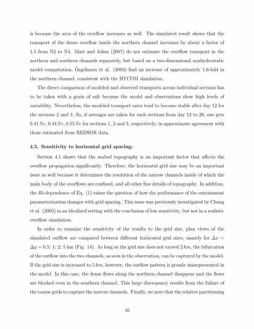
4.5. Sensitivity to horizontal grid spacing:

Section 4.1 shows that the seabed topography is an important factor that affects the

overflow propagation significantly. Therefore, the horizontal grid size may be an important

issue as well because it determines the resolution of the narrow channels inside of which the

main body of the overflows are confined, and all other fine details of topography. In addition,

the Ri-dependence of Eq. (1) raises the question of how the performance of the entrainment

parameterization changes with grid spacing. This issue was previously investigated by Chang

et al. (2005) in an idealized setting with the conclusion of low sensitivity, but not in a realistic

overflow simulation.

In order to examine the sensitivity of the results to the grid size, plan views of the

simulated outflow are compared between different horizontal grid sizes, namely for ∆x =

∆y = 0.5; 1; 2; 5 km (Fig. 14). As long as the grid size does not exceed 2 km, the bifurcation

of the outflow into the two channels, as seen in the observation, can be captured by the model.

If the grid size is increased to 5 km, however, the outflow pattern is grossly misrepresented in

the model. In this case, the dense flows along the northern channel disappear and the flows

are blocked even in the southern channel. This large discrepancy results from the failure of

the coarse grids to capture the narrow channels. Finally, we note that the relative partitioning

16

of the overflow between southern and northern channels is very sensitive to the horizontal

grid spacing as well. In particular, the preferred behavior in course-resolution cases is to

flow into the southern channel, because it is a more direct pathway, while diversion of part

of the overflow into the northern channel requires more precise resolution and dynamics.

A more detailed comparison is shown for salinity profiles computed from ∆x = ∆y =

0.5 km and ∆x = ∆y = 1 km (Fig. 15). It appears that the two different horizonal resolu-

tions generally generate consistent results, having small differences from each other. There-

fore, the variation in grid resolution may not greatly affect the results as long as it is fine

enough to resolve the channels. Results from ∆x = ∆y = 2 km and ∆x = ∆y = 5 km are

not plotted because the locations of the stations are not accurate in these cases.

In light of such significant dependence of topographic details to grid spacing, the sensitiv-

ity of the performance of Eq. (1) becomes clearly a secondary consideration. Specifically, if

the geometry is not accurate enough to represent the main flow pathways, the dynamics are

already considerably modified, and one cannot expect a mixing parameterization to rectify

the computation.

4.6. Effect of different entrainment schemes:

As investigated in sections 4.1 and 4.5, the seabed bottom topography and the horizon-

tal grid resolution are the factors that most significantly affect the model simulation results.

These geometric factors are important because the main pathways of the Red Sea over-

flows are characterized by relatively smaller scales compared to other overflows such as the

Mediterranean overflow or the Denmark Strait overflow. Also, the large-scale slope of the

bottom topography is about 1/3◦, which is two- to three-fold smaller than those in the other

overflows mentioned above. Therefore, the vertical mixing schemes that played an important

role in those outflows may act differently in the Red Sea overflow. In order to investigate

the impact of the vertical mixing in the isopycnal coordinate model employed herein, KPP,

a popular scheme used in many OGCMs, is used in addition to the main scheme TPX.

The KPP scheme has a number of components addressing different physical processes.

Of these, only the parameterization of shear-driven mixing in the form of eddy viscosity

and eddy diffusivity as functions of the local gradient Richardson number is relevant for this

17

study. The gradient Richardson number Ri is the ratio of the squared buoyancy frequency N 2

and the squared vertical shear, Ri = N 2

[

(

∂u∂z

)2

+(

∂v∂z

)2]

−1

. The vertical eddy diffusivity

is given by

Kshear = Kmax ×

[

1 − min(1 , (Ri

Ric))2

]3

, (3)

so that vertical diffusivity is zero when Ri ≥ Ric with Ric = 0.7. When Ri < Ric, vertical

diffusivity gradually increases to account for stronger mixing due to weaker stratification,

and at the limit of Ri = 0, mixing takes place with an intensity qualified by Kmax. Large

(1998) estimated the value of Kmax from large eddy simulations of the upper equatorial

Pacific, specifically finding Kmax =50 cm2s−1.

In Fig. 16 the propagation patterns resulting from KPP and TPX are compared in

terms of planview (top panels) as well as the profile view (bottom panels) of the salinity

distribution at day 10. Clearly, both schemes yield very similar patterns of the modeled

overflows. The propagation pattern differs slightly once the dense flows arrive at the Tadjura

Rift and start reaching neutral buoyancy while spreading horizontally by lateral mixing as

well. The similarity between the two mixing schemes is also confirmed using profile views.

The thicknesses of the overflows are almost same at every location along the channel and

show no significant difference between the two schemes.

In order to quantify the difference between the results of the two schemes, an error

function is used by normalizing the deviation of the simulated salinity profiles from the

observations as

Erri(t) =

√

√

√

√

j=N i

∑

j=1

[

Sri

model(j)− Sriobs(j)

]2

/N i

∆Sr, (4)

where Sri

model is the time-averaged model output of tracer (salinity) and Sriobs is the observed

value at station i, N i is the number of sampling points, and Erri(t) is the rms error nor-

malized by tracer ranges ∆Sr (∆S = 4.3 psu, ∆T = 11◦ C). In Fig. 17 the error function,

Erri(t) is plotted for the eight stations (N1 to N5, S1 to S3). It can be seen that errors are

reduced rapidly until t = 5 days, when they drop to less than 10 % of the tracer amplitude

range, and show little variation after that. Most striking is the similarity of Erri(t) between

18

KPP and TPX. Based on this analysis, the difference in the model results arising from the

choice of the vertical mixing parameterization is small compared to other, more significant

factors influencing the simulation, namely the resolution of the details of bottom topography

and vertical resolution of the overflow structure.

It should be noted that significant differences have been reported between KPP and TP

in the study by Chang et al. (2005) based on an idealized experimental setup, in which

the slope angle was θ = 3.5◦. It was put forth that this was due to the constant value of

Kmax, which was inadequate to provide the mixing needed in the gravity current flow over

such slopes. It appears that an order of magnitude smaller slopes in the Red Sea overflow

domain, namely θ ≈ 1/3◦ in the northern channel, ensure that this limitation of KPP is not

encountered in the present simulations.

4.7. Sensitivity to source water forcing:

Finally, the sensitivity of the results to changes in the inlet source water forcing is ex-

plored. This issue is important as the observational sampling in the Bab el Mandeb Strait

captured neither all the time variability (e.g., due to tides) nor the cross-sectional variations.

In order to develop some insight into consequences associated with uncertainties in source

water forcing, two additional experiments are carried out (with TPX and ∆x = ∆y = 1 km),

in which the water mass properties reaching control station T0 are varied. The forcing varia-

tion has been acomplished by changing the thickness of the bottom dense water mass inside

the artificial reservoir. Fig. 18 shows three different levels of outflow water mass at T0.

Stronger or weaker forcing is implemented by initializing with approximately ±15% thicker

or thinner outflow water height at this station.

The magnitude of this change is somewhat arbitrary as we do not know quantitatively the

uncertainties arising from spatial and time sampling. Nevertheless, the change is adequate to

provide some insight on the sensitivities of the system to source water forcing. The salinity

distributions in the northern channel remains insensitive to the source changes whereas

those in the southern channel exhibit a proportional response (Fig. 19). textcolorgreenThis

response seems a consequence of the implemented source thickness change of ±25 m (Fig.

18). This value is of the same order as a 30-m saddle height of the bifurcation point between

19

the channels relative to the floor of the main, northern channel. A thicker plume will more

readily spill over into the southern channel than a thinner one. It is, however, unclear if the

OGCM adequately captures the flow dynamics near the bifurcation point. Several factors,

such as the need for very high resolution (topography and discretization) and hydraulic

control including nonhydrostatic dynamics, need to be considered in future modeling efforts.

6. Summary and discussion:

Overflow dynamics constitute an important part of the ocean general circulation since

overflows supply most of the intermediate and deep water masses from spatially restricted

source areas, such as narrow straits. In addition, the source water mass properties are typi-

cally significantly modified on their path to neutral buoyancy and before joining the general

circulation via mixing processes taking place over small spatial and time scales (Price and

Baringer, 1994). Thus, overflows are considered to form important bottle necks in the gen-

eral circulation, and need to be explored and understood better in order to be incorporated

in OGCMs and ultimately in climate studies in a realistic way.

In this study, realistic simulations of the Red Sea overflow are attempted using HY-

COM and observational data set from REDSOX. To our knowledge, this is the first realistic

numerical investigation of the entire Red Sea overflow system. An important objective of

this study is to explore the requirements necessary to capture the dynamics of this over-

flow system using an OGCM. Previous investigations of other overflows revealed significant

differences from one another. Computations by Jungclaus and Mellor (2000), Papadakis et

al. (2003) and Xu et al. (2006) indicate that the entrainment parameterization is of critical

importance in modeling the Mediterranean Sea overflow. Its source water is dense enough to

sink to the bottom of the North Atlantic ocean, but the product waters in fact equilibrate at

intermediate depths (Baringer and Price, 1997a,b). Thus, small differences in entrainment

parameterizations are found to lead to significant changes in the properties and equilibrium

depth of the product water masses (Xu et al., 2006). In the case of the Denmark Strait

overflow, the overflow never detaches from the bottom, and lateral entrainment via quasi-

barotropic eddies appears to be important, in addition to vertical entrainment (Kase et al.,

2003; Tom Haine and Alistair Adcroft, 2006, personal communication). Fine-scale details

20

of bottom topography appear to exert a strong influence on the overflow in the Faroe Bank

Channel (Price, 2004; Ezer, 2006), whereas other factors such as tidal forcing and formation

of episodic cascades seem to be important in the dynamics of Antarctic overflows (Gordon

et al., 2004).

The REDSOX data set is used herein to initialize, force and validate the model results.

In particular, eight stations from the 2001 REDSOX winter cruise are used to assess the

model accuracy following the bifurcation of the overflow into the narrow channels. Also,

three sections crossing the entire overflow system are employed. The comparison of the

model results with data is constrained to the phase before the overflows fill the intermediate

depths in the Tadjura Rift.

As the simulation is started from a lock-exhange at the Bab el Mandeb Strait, there

is a transient phase of overflow propagation before a statistical steady state is achieved.

It is noted that the initial propagation speed of the modeled overflow is much smaller, by

a factor of two on average, than the theoretical interfacial speed of internal waves. It is

shown that this is due to the fact that the initial overflow propagation is impeded by rough

topography. A similar effect of rough topography on overflow propagation speed was also

noticed in nonhydrostatic simulations by Ozgokmen et al. (2004b, their Fig. 2a vs 2d).

A comprehensive comparison of salinity, temperature and velocity profiles, and volume

transport in the southern and northern channels, as well as across three sections crossing

the entire overflow system from the model and observations is carried out. The agreement

between the model and data appears reasonably satisfactory. The main contribution of this

study is to quantify the sensitivity of the results to various modeling choices. It is found that

by far the most important issue in modeling the Red Sea overflow is the resolution of critical

topographic features, namely both the southern and northern channels with their ≈ 5 km

width, and in particular the area near the bifurcation point of these channels. The popular

ETOPO5 data set contained significant errors, and thus multibeam echosoundings with 200

m resolution were used for these critical areas. A horizontal grid spacing of 1 km, or finer,

is required to provide adequate dense water flow into the northern channel and to reproduce

a realistic overflow bifurcation and distributions of water mass properties. At coarser reso-

lutions, first the flow in the northern channel and then the southern channel is blocked, and

21

the Red Sea overflow becomes grossly misrepresented. Even with high horizontal resolution,

it is a challenge to achieve an accurate partitioning of the flow between the two channels.

The narrow multi-channel topography significantly increases the challenge of parameterizing

entire overflows for climate models, in which the typical resolution is 100 km at the present

time. Nevertheless, it seems encouraging that the model provides reasonable results at a

marginal resolution of the channels. It is shown that the salinity distributions inside the

channels are then affected by the forcing in the Strait, such that the modeled dense fluid

has a stronger tendency to flow down the southern than the northern channel. A highly

accurate topographic data set and very high model resolution may be required to achieve

a higher degree of realism. The importance of the resolution of narrow channels in bottom

topography is also evident in the idealized (Ezer, 2006) and realistic (Riemenschneider and

Legg, 2007) numerical studies of the Faroe Bank Channel overflow. Alternatively, missing

dynamics, such as time-dependent forcing and nonhydrostatic effects may play an important

role near the bifurcation point. Unlike in previous studies of other overflows (e.g., Papadakis

et al., 2003; Chang et al., 2005; Xu et al., 2006), the sensitivity of the simulations to the

choice of the entrainment parameterization, either TPX or KPP, is found to be small. Nev-

ertheless, a realistic entrainment parameterization is still needed. It is estimated that the

volume transport of the overflow increases from 0.41 Sv to 0.55 Sv from section 1 to section

3, in approximate agreement with the estimates from observations.

This study indicates that a number of challenges remain in modeling overflows. The first

is the challenge of parameterizing the effect of the Red Sea overflow on the general circu-

lation, since it is not feasible in the foreseeable future that the fine-scale channels will be

resolved in climate studies. Thus it is not clear how the effect of topographic pathways can or

should be lumped into mixing parameterizations. The second is the inefficiency of numerical

methods based on finite-difference schemes when extreme sitations are encountered, in which

the dynamics are constrained to very small areas (channels) whereas computations remain

distributed. Alternative numerical methods with higher geometrical flexibility, for example

those based on the finite-element method with adaptive or unstructured grids, should also be

considered. Third is the methodological question of assessing the fidelity of a numerical sim-

ulation from typically small, sparse, and non-synoptic observational data sets. Methods for

22

incorporating the uncertainty in the subsampling and time-space variability of observational

data in assessing the fidelity of a numerical simulation need to be developed.

Acknowledgments

We greatly appreciate the support of National Science Foundation via grant OCE 0336799

for the Climate Process Team on Gravity Current Entrainment, as well as through OCE-

9819506, OCE-9818464 and OCE-0351116 for the REDSOX. The multibeam echosounder

data from the R/V L’Atlante were generously provided by Philippe Huchon. These, as well

as the echosoundings from the two REDSOX cruises on the R/V Knorr and the R/V Maurice

Ewing, were worked up and kindly shared with us by Steve Swift. We thank Silvia Matt

for helping us with merging the high-resolution and low-resolution bottom topography data

sets, Bill Johns and Marcello Magaldi for their constructive criticism. We also thank the

two anonymous reviewers for their constructive comments, which helped greatly improve the

manuscript.

References

Baines, P. G., 2001: Mixing in flows down gentle slopes into stratified environments. J.

Fluid Mech., 443, 237–270.

Baines, P. G., 2005: Mixing regimes for the flow of dense fluid down slopes into stratified

environments. J. Fluid Mech., 443, 245–267.

Baringer, M. O., and J. F. Price, 1997(a): Mixing and spreading of the Mediterranean

outflow J. Phys. Oceanogr, 27(8), 1654–1677.

Baringer, M. O., and J. F. Price, 1997(b): Momentum and energy balance of the Mediter-

ranean outflow. J. Phys. Oceanogr, 27(8), 1678–1692.

Bleck, R., 2002: An oceanic general circulation model framed in hybrid isopycnic-Cartesian

coordinates. Ocean Modelling, 4, 55-88.

Bower, A. S., H. D. Hunt, and J. F. Price, 2000: Character and dynamics of the Red Sea

and Persian Gulf outflows. J. Geophys. Res., 105, 63876414.

Bower, A. S., D. M. Fratantoni, W. E. Johns, and H. Peters, 2002: Gulf of Aden eddies

and their impacts on Red Sea Water. Geophys. Res. Lett., 29, 2025,

doi:10.1029/2002GL015342

23

Bower, A. S., W. E. Johns, D. M. Fratantoni, and H. Peters, 2005: Equilibration and cir-

culation of Red Sea Outflow Water in the western Gulf of Aden. J. Phys. Oceanogr.,

35, 1963-1985

Britter, R. E., and P.F. Linden, 1980: The motion of the front of a gravity current travelling

down an incline. J. Fluid Mech., 99, 531–543.

Brydon, D., S. Sun, and R. Bleck, 1999: A new approximation of the equation of state for

sea water, suitable for numerical ocean models. J. Geophys. Res., 104, 1537-1540.

Cenedese, C., J.A. Whitehead, T.A. Ascarelli, and M. Ohiwa, 2004: A Dense Current Flow-

ing down a Sloping Bottom in a Rotating Fluid. J. Phys. Oceanogr., 34(1), 188–203.

Chang, Y. S., X. Xu, T. M. Ozgokmen, E. P. Chassignet, H. Peters, and P. Fischer, 2005:

Comparison of gravity current mixing parameterizations and calibration using a high-

resolution 3D nonhydrostatic spectral element model. Ocean Modelling, 10, 342–368.

Chassignet, E.P., L.T. Smith, G.R. Halliwell, and R. Bleck, 2003: North Atlantic simulation

with the HYbrid Coordinate Ocean Model (HYCOM): Impact of the vertical coordi-

nate choice, reference density, and thermobaricity. J. Phys. Oceanogr., 33, 2504-2526.

Ellison, T. H., and J. S. Turner, 1959: Turbulent entrainment in stratified flows. J. Fluid

Mech., 6, 423–448.

Ezer, T., 2006: Topographic influence on overflow dynamics: idealized numerical simula-

tions and Faroe Bank Channel overflow. J. Geophys. Res., 111, C02002,

doi:10.1029/2005JC003195.

Ezer, T., 2005: Entrainment, diapycnal mixing and transport in three-dimensional bottom

gravity current simulations using the Mellor-Yamada turbulence scheme. Ocean Mod-

elling, 9, 151–168.

Ezer, T., and G.L. Mellor, 2004: A generalized coordinate ocean model and comparison of

the bottom boundary layer dynamics in terrain-following and in z-level grids. Ocean

Modelling, 6, 379–403.

Fernando, H.J.S., 1991: Turbulent mixing in stratified fluids. Ann. Rev. Fluid Mech., 23,

455–494.

Girton, J. B., T. B. Sanford, and R. H. Kase, 2001: Synoptic sections of the Denmark

Strait Overflow. Geophys. Res.Lett., 28(8), 1619–1622.

Girton, J. B., and T. B. Sanford, 2003: Descent and modification of the overflow plume in

the Denmark Strait. J. Phys. Oceanogr., 37(7), 1351–1364.

24

Gordon, A. L., E. Zambianchi, A. Orsi, M. Visbeck, C. F. Giulivi, T. Whitworth, and G.

Spezie, 2004: Energetic plumes over the western Ross Sea continental slope. Geophy.

Res. Lett., 31(21), Art. No. L21302.

Hallberg, R., 2000: Time integration of diapycnal diffusion and Richardson number de-

pendent mixing in isopycnal coordinate ocean models. Mon. Wea. Rev., 128(5),

1402–1419.

Halliwell, G.R., 2004: Evaluation of vertical coordinate and vertical mixing algorithms in

the HYbrid-Coordinate Ocean Model (HYCOM). Ocean Modeling., 7, 285-322.

Hallworth, M. A., H.E. Huppert, J.C. Phillips, and R.S.J. Sparks, 1996: Entrainment into

two-dimensional and axisymmetric turbulent gravity currents. J. Fluid Mech., 308,

289-311.

Hebert, H., L. Audin, C. Deplus, P. Huchon, and K. Khanbari, 2001: Lithospheric structure

of a nascent spreading ridge inffered from gravity data. The Western Gulf of Aden. J.

Geophys. Res. B: Solid Earth, 106, 26345-26363.

Jungclaus, J. H., and G. Mellor, 2000: A three-dimensional model study of the Mediter-

ranean outflow. J. Mar. Sys., 24, 41-66.

Kase, R. H., J.B. Girton, and T.B. Sanford, 2003: Structure and variability of the Denmark

Strait Overflow: Model and observations. J. Geophys. Res., 108(C6), Art. No.3181

Killworth, P. D., 1977: Mixing on the Weddell Sea continental slope. Deep-Sea Res., 24,

427448.

Large, W.G., 1998: Modeling and parameterizing ocean planetary boundary layer. In

Chassignet, E. P., Vernon, J. (Eds) Ocean modeling and parameterization. Kluwer,

pp. 45-80.

Large, W.G., and P. R. Gent, 1999: Validation of vertical mixing in an equatorial ocean

model using large eddy simulations and observations. J. Phys. Oceanogr., 29, 449-464.

Large, W. G., J.C. McWilliams, and S.C. Doney, 1994: Oceanic vertical mixing: A review

and a model with a nonlocal boundary layer parameterization. Rev. Geophys., 32,

363-403.

Legg, S., R.W. Hallberg, and J.B. Girton, 2006: Comparison of entrainment in overflows

simulated by z-coordinate isopycnal and non-hydrostatic models. Ocean Model. Ocean

Modelling, 11, 69–97.

25

Matt, S., and W.E. Johns, 2007: Transport and entrainment in the Red Sea outflow plume.

J. Phys. Oceanogr., in press.

Matt, S., 2004: Transport and entrainment in the Red Sea outflow. M.S. thesis, University

of Miami, 93 pp.

Monaghan, J. J., R.A.F. Cas, A.M. Kos, and M. Hallworth, 1999: Gravity currents de-

scending a ramp in a stratified tank. J. Fluid Mech., 379, 39–70.

Morcos, S. A., 1970: Physical and chemical oceanography of the Red Sea. Oceanogr. Mar.

Biology Ann. Rev., 8, 73–202.

Murray, S. P., and W. E. Johns, 1997: Direct observations of seasonal exchange through

the Bab el Mandab Strait. Geophys. Res. Lett., 24(21), 2557–2560.

Ozgokmen T.M., and E. Chassignet, 2002: Dynamics of two-dimensional turbulent bottom

gravity currents. J. Phys. Oceanogr., 32, 1460–1478.

Ozgokmen T.M., W.E. Johns, H. Peters and S. Matt, 2003: Turbulent mixing in the Red

sea outflow flume from a high-resolution nonhydrostatic model. J. Phys. Oceanogr.,

33(8), 1846–1869.

Ozgokmen T.M., P.F. Fischer, J. Duan and T. Iliescu, 2004a: Three-dimensional turbulent

bottom density currents from a high-order nonhydrostatic spectral element model. J.

Phys. Oceanogr., 34(9), 2006–2026.

Ozgokmen T.M., P.F. Fischer, J. Duan and T. Iliescu, 2004b: Entrainment in bottom

gravity currents over complex topography from three-dimensional nonhydrostatic sim-

ulations. Geophys. Res. Let.., 31, L13212

Ozgokmen T.M., P.F. Fischer, and W.E. Johns, 2006: Product water mass formation by

turbulent density currents from a high-order nonhydrostatic spectral element model.

Ocean Modelling., 12, 237–267.

Papadakis, M. P., E. P. Chassignet, and R. W. Hallberg, 2003: Numerical simulations

of the Mediterranean Sea outflow: Impact of the entrainment parameterization in an

isopycnic coordinate ocean model. Ocean Modelling, 5, 325–356.

Peters, H., and W.E. Johns, 2005: Mixing and entrainment in the Red Sea outflow plume.

II. turbulence characteristics. J. Phys. Oceanogr., 35, 584–600

Peters, H., W.E. Johns, A.S. Bower, and D.M. Fratantoni, 2005: Mixing and entrainment

in the Red Sea outflow plume. I. plume structure. J. Phys. Oceanogr., 35, 569–583

26

Price, J. F., 2004: A process study of the Faroe Bank Channel overflow. Geophys. Res.

Abstracts, 6, 07788.

Price, J. F., and M. O. Baringer, 1994: Outflows and deep water production by marginal

seas. Prog. Oceanogr., 33, 161–200.

Riemenschneider, U. and S. Legg, 2007: Regional simulations of the Faroe Bank Channel

overflow in a level model. Ocean Modelling, in press.

Siedler, G., 1969: General circulation of water masses in the Red Sea. In Hot Brines

and Recent Heavy Metal Deposits in the Red Sea, eds: E.T. Degens and D.A. Ross,

Spronger, 131–137.

Simpson, J. E.., 1969: A comparison between laboratory and atmospheric density currents.

Quart. J. Roy. Meteor. Soc., 95, 758–765

Simpson, J. E.., 1982: Gravity current in the laboratory, atmosphere, and ocean. Ann.

Rev. Fluid Mech., 14, 213–234

Simpson, J. E.., 1987: Gravity currents: In the environment and laboratory. John Wiley

and Sons, New York, 244pp

Smith, W. H. F., and D. T. Sandwell, 1997: Global seafloor topography from satellite al-

timetry and ship depth soundings. Science, 277, 195-196.

Sofianos, S. S., W. E. Johns, and S. P. Murray, 2002: Heat and freshwater budgets in the

Red Sea from direct observations at Bab el Mandeb. Deep Sea-Res. Pt II, 49, 1323–

1340.

Strang, E. J., and H.J.S. Fernando, 2001: Turbulence and Mixing in Stratified Shear Flows

J. Fluid Mech., 428, 349–386

Turner, J. S., 1986: Turbulent entrainment: The development of the entrainment assump-

tion, and its applications to geophysical flows. J. Fluid Mech., 173, 431–471.

Willebrand, J., B. Barnier, C. Boning, C. Dietrich, P. D. Killworth,C. L. Provost, Y. Jia,

J. Molines, and A. L. New, 2001: Circulation characteristics in three eddy-permitting

models of the North Atlantic. Progr. Oceanogr., 48, 123-161.

Xu, X., Y.S. Chang, H. Peters, T.M. Ozgokmen, and E.P. Chassignet, 2006: Parameteri-

zation of gravity current entrainment for ocean circulation models using a high-order

3D nonhydrostatic spectral element model. Ocean Modelling, 14, 19-44.

27

40˚E 42˚E 44˚E 46˚E 48˚E 50˚E 52˚E 54˚E 56˚E 58˚E 60˚E

12˚N

14˚N

16˚N

18˚N

Saudi Arabia

Yemen

GULF OF ADEN

Oman

Arabian Sea

Somalia

BAM Strait

RED

SEA

RED

SEA

Sec1

Sec2

Sec3

S3

S1

S2

N2N4

N5

N1

N3

T0

T1

P1P2 P3

Sec4Sec5

43 43.5 44 44.5

11.6

11.8

12

12.2

12.4

12.6

12.8

13

−0.5

0

0.5

1

1.5

Figure 1: (Upper panel) Chart showing the geographical location of the Red Sea, the Bab el Mandeb

Strait and the Gulf of Aden. The box at the Bab el Mandeb Strait marks the boundary of the

computational domain. (Lower panel) Enlarged view of the computational domain (in latitude and

longitude). Depths (in km) show the bottom topography. The dotted lines indicate the northern

and southern channels, the main routes of the Red Sea outflow. T0 denotes the station south of the

Bab el Mandeb Strait and south of an artifical reservoir created north of 12.7◦N. Profiles from T0

are used to validate the source water outflow properties. T1 denotes the station used to initialize

the ambient stratification, and it is outside of the outflow pathways. N1 to N5 denote the selected

measurement locations along the northern channel, and S1 to S3 are the selected locations along

the southern channel for model validation. In addition, three sections across the outflow plume,

Sec1 to Sec3, are also used to compare HYCOM results to those from REDSOX.

28

35 36 37 38 39 40

0

0.1

0.2

0.3

dept

h, k

m

(a) Salinity, T0

t=0 (day)

t=1

t=20

10 15 20 25 30

(b) Temperature, T0

t=0 (day)

t=1

t=20

−1 −0.5 0 0.5 1

0

0.1

0.2

0.3

dept

h, k

m

(c) Velocities, T0

t=0

t=1

t=1

t=20t=20

24 25 26 27 28

(d) Density, T0

t=0

t=1

t=20

Figure 2: Time evolution of (a) salinity (in psu), (b) temperature (in ◦C), (c) velocity (in

m/s), and (d) density (in σθ) profiles at station T0. Red and blue solid lines show the

REDSOX profiles. Solid, dashed and dashed-dotted lines show HYCOM profiles at 0, 1 and

20 days, respectively. In (c) the red line shows u-velocities (positive eastward) and blue line

shows v-component (positive northward).

29

Figure 3: Plan views of the time evolution (t = 0, 2, 5, 7, 10, and 20 days) of the outflow

propagation in terms of the salinity averaged over layers 10 to 14, which contain the overflow

water masses.

30

Southern channelt = 1(day)

t = 3

t = 5

t = 7

t = 9

0 50 100 150

Northern channel t = 1(day)

km

psu

0.10.50.91.3

t = 3

km

0.10.50.91.3

t = 5

km

0.10.50.91.3

t = 7

km

0.10.50.91.3

t = 9

km

0 50 100 150

0.10.50.91.3

35363738

Figure 4: Profile views of the time evolution (t = 1, 3, 5, 7, and 9 days) of the overflow

salinity distribution along the northern channel (left panels) and southern channel (right

panels). The distance starts from the southern exit of the Bab el Mandeb Strait.

31

10 20 30 40 50 60 70 80 90

0.2

0.4

0.6

0.8

1(a) Propagation speed

UF, m

/s

10 20 30 40 50 60 70 80 90

0.1

0.2

0.3

0.4

0.5

km

km

(b) Outflow propagation, profile (northern channel)

psu

35 36 37 38

Figure 5: (a) Initial propagation speed of the modeled overflow, and (b) section of bottom

topography along the northern channel. Note that the propagation speed is significantly

reduced at locations where rough bottom topography is encountered.

32

36 38 40

0

0.1

0.2

0.3

z, k

m

(a) St#= N1

36 38 40

0

0.2

0.4

(b) St#= N2

36 38 40

0

0.2

0.4

(c) St#= N3

36 38 40

0

0.2

0.4

0.6

(d) St#= N4

36 38 40

0

0.2

0.4

0.6

z, k

m

psu

(e) St#= N5

36 38 40

0

0.1

0.2

psu

(f) St#= S1

36 38 40

0

0.1

0.2

0.3

psu

(g) St#= S2

36 38 40

0

0.1

0.2

0.3

0.4

psu

(h) St#= S3

Figure 6: Comparison of salinity profiles in the northern channel (N1 to N5) and southern

channel (S1 to S3) stations. Solid/black lines: REDSOX profiles vertically averaged to obtain

mean values corresponding to the 16 layers in HYCOM. Solid/red lines: HYCOM profiles

(TPX, ∆x = ∆y = 1 km) which are time averaged from day 10 to 20. Dashed/red lines:

95% confidence intervals of computed profiles indicating time variability. Solid/blue line:

model initialization from T1 (note that the water depth is different at the station location

but the initialization profiles are identical at the same level).

33

km

Modeled (TPX) − Northern Channel

70 80 90 100 110 120 130 140 150

0

0.5

1

70 80 90 100 110 120 130 140 150

0

0.5

1

distance along the northern channel (km)

km

Observed (REDSOX)

psu

psu

N1 N2 N3 N4 N5

35

36

37

38

35

36

37

38

Figure 7: Comparison of salinity distributions along the northern channel from HYCOM

simulation (upper panel) and REDSOX observations (lower panel). In the lower panel,

the continous distribution is obtained by interpolating REDSOX profiles from nine stations

marked by the green lines.

34

km

Modeled (TPX) − Southern Channel

60 65 70 75 80 85 90 95

0

0.2

0.4

0.6

60 65 70 75 80 85 90 95

0

0.2

0.4

0.6

distance along the southern channel (km)

km

Observed (REDSOX)

psu

psu

S1 S2 S3

35

36

37

38

35

36

37

38

Figure 8: Same as Fig. 7 but for the southern channel.

35

(a) Section 1

z, k

m

0.1

0.2

0.3

(b) Section 2

z, k

m

0.2

0.4

(c) Section 3

x, km

z, k

m

0 20 40 60 80 100

0.2

0.4

0.6

36

38

(d) Section 1

z, k

m

0.1

0.2

0.3

(e) Section 2

z, k

m0.2

0.4

(f) Section 3

x, km

z, k

m

0 20 40 60 80 100

0.2

0.4

0.6

36

38

40

Figure 9: Salinity distributions across the outflow plume from REDSOX at (a) section 1,

(b) section 2, and (c) section 3, and from HYCOM at (d) section 1, (e) section 2, and (f)

section 3.

36

0 5 10 15 20

0.2

0.4

0.6

0.8

1

z, k

m

x, km

Section 4 (Northern Channel, TPX)

0 5 10 15 20

0.2

0.4

0.6

0.8

1

z, k

m

x, km

Section 5 (Southern Channel, TPX)

36 38 40

0.2

0.4

0.6

0.8

1

St# = P1

psu

36 38 40

0.2

0.4

0.6

0.8

1

St# = P2

psu36 38 40

St# = P3

psu

35

36

37

38

39

Figure 10: Salinity distributions along sections crossing the northern (Section 4) and the

southern channel (Section 5) at the interface with the Tadjura Rift. Also, the comparison

of salinity profiles at stations P1, P2, and P3 between observed (black lines) and computed

(red lines) profiles. Refer to Fig. 1 for locations of Section 4, Section 5, P1, P2 and P3. The

horizontal size of the cells corresponds to the horizontal grid spacing (1 km) and the vertical

size to the layer thickness. The layers also indicate the density classes.

37

0 0.5 1

0

0.1

0.2

0.3

z, k

m

(a) St#= N1

0 0.5 1

0

0.2

0.4

(b) St#= N2

0 0.5 1

0

0.2

0.4

(c) St#= N3

0 0.5 1

0

0.2

0.4

0.6

(d) St#= N4

0 0.5 1

0

0.2

0.4

0.6

z, k

m

m/s

(e) St#= N5

0 0.5 1

0

0.1

0.2

m/s

(f) St#= S1

0 0.5 1

0

0.1

0.2

0.3

m/s

(g) St#= S2

0 0.5 1

0

0.1

0.2

0.3

0.4

m/s

(h) St#= S3

Figure 11: Comparison of the streamwise velocity profiles in the northern channel (N1 to

N5) and southern channel (S1 to S3) stations. Solid/black lines: REDSOX profiles vertically

averaged to obtain mean values corresponding to the 16 layers in HYCOM. Solid/red lines:

HYCOM profiles (TPX, ∆x = ∆y = 1 km) which are time averaged from day 10 to 20.

Dashed/red lines: 95% confidence intervals of computed profiles indicating time variability.

Solid/blue line: model initialization.

38

0 2 4 6 8 10

0.2

0.25

0.3

0.35

0.4

0.45

0.5

0.55

km

km

(a) Sal. Y−Z plane, nz=16 layers

−1 3

2426

15

432

5130

8

223

249

35

35.5

36

36.5

37

37.5

38

38.5

39

39.5

40

0 2 4 6 8 10

0.2

0.25

0.3

0.35

0.4

0.45

0.5

0.55

km

km

(b) Sal. Y−Z plane, nz=12 layers

1

−

−

432

21

445

15

225

−

35

35.5

36

36.5

37

37.5

38

38.5

39

39.5

40

Figure 12: Cross-sectional view of the salinity distributions at each cross-sectional cell cross-

ing the northern channel at station N3 and t = 20 days from standard model experiment

with 16 layers (upper panel) and an experiment with 12 layers (lower panel). The superim-

posed numbers denote the streamwise velocity magnitude in each cell (in cm/s and positive

streamwise).

39

0 5 10 15 200

0.1

0.2

0.3

0.4

0.5

0.6

0.7

Vol

ume

tran

spor

t, Q

Elapsed day

0.35 SV

0.42 SV

0.56 SV

Figure 13: Volume transport Q of the Red Sea outflows at sections 1 (red), 2 (blue) and

3 (green) in comparison with those estimated from REDSOX observations (black, dashed),

which are 0.35 Sv (section 1), 0.42 Sv (section 2), and 0.56 Sv (section 3).

40

Figure 14: Outflow patterns resulting from different grid sizes, as depicted using the salinity

distribution in layer ten and at t = 20 days. (a) ∆x = 0.5 km, (b) ∆x = 1 km, (c) ∆x = 2 km,

(d) ∆x = 5 km.

41

36 38 40

0

0.1

0.2

0.3

z, k

m

(a) St#= N1

36 38 40

0

0.2

0.4

(b) St#= N2

36 38 40

0

0.2

0.4

0

0.2

0.4

(c) St#= N3

36 38 40

0

0.2

0.4

0.6

(d) St#= N4

36 38 40

0

0.2

0.4

0.6

z, k

m

psu

(e) St#= N5

36 38 40

0

0.1

0.2

0

0.1

0.2

psu

(f) St#= S1

36 38 40

0

0.1

0.2

0.3

psu

(g) St#= S2

36 38 40

0

0.1

0.2

0.3

0.4

psu

(h) St#= S3

Figure 15: Comparison of salinity profiles from different horizontal grid spacings, ∆x = 1

km (solid) and ∆x = 0.5 km (dashed).

42

Figure 16: Comparison of the modeled salinity distribution from KPP (left panels) and TPX

(right panels) in the plan view (top panels, model layer 10) and the profile view (bottom

panels) along the northern channel.

43

Ela

psed

day

(b) TPX

S3 S2 S1 N1 N2 N3 N4 N5Stations

5

10

15

20

Ela

psed

day

(a) KPP

5

10

15

20

0

0.1

0.2

0.3

0.4

0

0.1

0.2

0.3

0.4

Figure 17: Time evolution of Erri(t) of computed salinity profiles at eight stations along the

northern and southern channels using (a) KPP and (b) TPX.

44

35 36 37 38 39 40

0

0.05

0.1

0.15

0.2

0.25

0.3

0.35

dept

h, k

m(a) Salinity, T0

psu

Figure 18: The modeled salinity profiles at station T0 corresponding to intermediate forcing

(solid line), strong forcing (dashed line) and weak forcing (dashed-dotted line). Red/solid

line shows the REDSOX profile.

45

36 38 40

0

0.1

0.2

0.3

z, k

m

(a) St#= N1

36 38 40

0

0.2

0.4

(b) St#= N2

36 38 40

0

0.2

0.4

(c) St#= N3

36 38 40

0

0.2

0.4

0.6

(d) St#= N4

36 38 40

0

0.2

0.4

0.6

z, k

m

psu

(e) St#= N5

36 38 40

0

0.1

0.2

psu

(f) St#= S1

36 38 40

0

0.1

0.2

0.3

psu

(g) St#= S2

36 38 40

0

0.1

0.2

0.3

0.4

psu

(h) St#= S3

Figure 19: Sensitivity of modeled salinity profiles in the northern channel (N1 to N5) and

southern channel (S1 to S3) stations to changes in the forcing profiles shown in Figure 18.

46