numerical simulation of the zeeman eﬀect from laser...

Numerical Simulation of the Zeeman Effect from

Laser-induced Fluorescence of Neutral Xenon

IEPC-2007-254

Presented at the 30th International Electric Propulsion Conference, Florence, Italy

September 17-20, 2007

Baılo B. Ngom,

Timothy B. Smith,

Wensheng Huang,

and Alec D. Gallimore

University of Michigan, Ann Arbor, MI 48109

We present a numerical method for solving the components of magnetic field intensities

relative to the axis of a tunable continuous-wave diode laser, which induces fluorescence

from xenon particles downstream of a Hall thruster. The algorithm uses a non-linear least-

squares error minimization techique based on the interior-reflective Newton approach for

large scale optimization problems to resolve magnetic field components from the absorption

spectrum of the particles undergoing 6S′ [1/2] → 6P ′ [3/2] transition at 834.682 nm-vacuum.

Aside from fine structure, the coupling between the species inherent hyperfine structure

and Zeeman Effect induced by an external magnetic field characterize the absorption line

spectrum. Our fitting model uses Bachers method of calculating Zeeman-hyperfine en-

ergy splitting and intensities of σ and π-transition lines, respectively, corresponding to

perpendicular and parallel exciting light polarizations. Lorentz-Doppler broadening of the

transition-line spectrum models to good accuracy measured spectra of neutral xenon in

an opto-galvanic cell subject to various external magnetic field intensity settings. These

latter measurements also validate our routine for minimizing the error between predicted

and measured absorption line spectra for optimal magnetic field intensities. Voigt-profile

modeling of line spectra makes it possible to estimate plasma kinetic temperature assum-

ing elastic collisions. These efforts precede our ultimate goal of sketching the magnetic

field distribution in a Hall thruster plume via application of the non-linear solver to neu-

tral and ion absorption lineshapes resulting from diode laser-induced fluorescence spectral

data. A spatial distribution of magnetic field intensity will help better understand failure

mechanisms in Hall thrusters necessarily to improvements in the design of thrusters.

1The 30th International Electric Propulsion Conference, Florence, Italy


I. introduction

Studies of electric thruster topologies have thus far relied on software-based modeling and physical probe-based measurements. Both these methods have limited field-mapping capabilities. In the former, the mod-eling is restricted to a vacuum environment of a ”cold” thruster that only generates a magnetic field. Alone,such a configuration, does not make possible any prediction on the interaction betweeen magnetic field andplasma. When combined with physical probing, vacuum field simulations do, to a certain extent, allow suchstudy. However, such measurements are intrusive due to the often non-negligible level of field contaminationinduced by current carrying physical probes12 .? This makes probe-size reduction to sub-millimeter magni-tudes the main recourse to reducing intrusiveness, but at the expense of higher sensitivity to failure. Thatis why, there has been growing interest in laser-induced fluorescence (LIF); the non-intrusive nature of thisoptical technique makes it an attractive for estimating magnetic field topology in electric thruster dischargesthrough spectral analysis. When subject to the external effect of field-generating thruster-magnets, energylevels of plasma-discharge particles split; thereby, affecting LIF spectra. In this work, we apply an exactnon-linear model to capture the Zeeman effect on the hyperfine structure of neutral xenon (Xe I) to modelthe effect of an external magnetic field on the species’ absorption spectra as they undergo excitation by alaser-beam polarized perpendicularly with respect to the field direction. In anticipation of Hall-thruster LIFdata exhibiting Zeeman splitting, we limit this preliminary work to the simpler case of an opto-galvanic cellimmersed within the external magnetic field produced by Helmholtz coils. Successful spectral data fitting ofthe model prompted the development of a magnetic field intensity and kinetic temperature solver, which wevalidate in this work using optogalvanic spectra measurements at various field intensity levels spanning [30,300] Gauss14—a practical intensity range reflecting field magnitudes in Hall-thrusters.

II. Theory of the non-linear Zeeman effect on hyperfine structure

Zeeman effect refers to a splitting of an atom’s energy-levels that occurs when a magnetic field is externallyapplied to it. More fundamentally, it results from interactions of the magnetic field with momenta associatedwith orbital motions of a nucleus and electrons. In the classical world, an analogous phenomenon is themechanical moment exerted on a current carrying circular wire along a direction normal to surface intersectingmagnetic field lines. A theory dating back to the 1930s and developed by Sommerfeld, Heisenberg, Lande, andPauli (cited in4) accurately models the zeeman effect on a spinning spherical charged body in orbital motionin a central force field and under an externally applied magnetic field using a complex matrix formulation. Todescribe the theory, Darwin uses the simpler formulation of wave-mechanics .4,5 An application of the theoryto natural elements is found in,1 in which Bacher computes splittings of thallium and bismuth hyperfine linesin the 300-500 nm wavelength range and successfully validates it against observed spectra. Though useful,the theory has been, for the most part, ignored among the engineering community due to the complex natureof computations involved for elements with high momentum quantum numbers. As a recourse, a commontrend has been to use approximative methods suited for low and high magnetic field intensities; These arerespectively termed Pashen-Back and Anomalous Zeeman models.Modern days’ advances in computing capabilities, render modeling of the Zeeman effect on the hyperfinestructure of hydrogenic element a trivial task; Still a good grasp and, hence, application of the exact theoryto a specie like xenon, which consists of isotopes with and without hyperfine structure requires a briefintroduction to the two approximative models of relevance to this work.

A. Approximative models in high and low-field limiting cases

Nuclear spin imposes a two-level categorization of approximative models more thoroughly described in.7

1. The linear Zeeman and Pashen-Back effects on the hyperfine structure

The Zeeman effect on the hyperfine applies to elements with non-zero nuclear spin subject to low externalmagnetic field intensities. In the vector representation, the model predicts a precession of the total angularmomentum (~F resulting from IJ-coupling) of the atomic system about the direction of the magnetic field

lines ( ~B). Combined with the quantized nature of ~F , this precession leads to in a magnetic moment µM

proportional to a new quantum number M . The presence of quantized magnetic moments, in turn, gives riseto potential energies corresponding to new energy states resulting from F-levels’ splittings. As expressed in



the following selection rules, F and M can only increase or decrease by 1 and span closed intervals:

|I − J | ≤ F ≤ I + J with ∆F = ±1 (II.1)

−F ≤ M ≤ +F with ∆M = ±1 (II.2)

The splitting of lines due to a field intensity B is given by:

∆E = µMB = (gF µBM)B, (II.3)

where gF , the Lande-factor, is proportional to electronic and nucleic Lande-factors gJ and gI , respectively.The other approximation results from the Pashen-Back effect on the hyperfine structure that applies tohigh external field intensities exerted on non-zero nuclear spin species. In this case, the potential also causessplitting of F-levels but arises from a lifting of IJ-coupling, which leads to independent precession of electronicand nucleic momenta about the field. As the field intensity increases, the angle between the direction ofthe field and the resulting quantized magnetic moment vectors µMJ

and µMI(respectively associated with a

single valence electron’ orbital motion and nucleus’ spin) increases. The magnitudes of the quantized vectorsare proportional to quantum numbers MJ and MI ; which, as in the low-field approximation, obey specificselection rules (refer to equations (II.12a) and (II.12b)).

−J ≤ MJ ≤ J with ∆MJ = ±1 (II.4)

−I ≤ MI ≤ I with ∆MI = ±1 (II.5)

2. The Anomalous Zeeman model

According to the Anomalous Zeeman theory, application of an external magnetic field of intensity B to xenonspecies without nuclear spin results in splitting J energy-levels into new MJ-levels. The energy displacementsof these levels (eq. II.6) about a parent J-level are proportional to B and a magnetic moment µMJ

; which inturn, is proportional to the quantum number MJ , whose admissible values are found from the selection rulesin equation (II.12a). According to the vector model, J-level splitting results from various possible projectionsof the total angular momentum of the electron along the direction of the magnetic field as the momentumvector precesses about the latter while orbiting the nucleus. For such species, energy splittings solely dependon the quantum number MJand the magnetic field intensity B, as indicated the following equation:

∆E = gJMJH (II.6)

As shown below, the following simple algebraic formulas yield line intensities for J → J + 1 transitions:

4(J2 − MJ

2) for M → M (II.7a)

(J − MJ + 1)(J − MJ + 2) M → M − 1 (II.7b)

(J + MJ + 1)(J + MJ + 2) M → M + 1 (II.7c)

All quantum numbers in the above equations are associated to initial states a.The Anomalous Zeeman theory is considered exact when applied to hydrogenic elements with no nuclearspin. But, at high magnetic field intensities, it consistutes a linear approximation for modeling spectra ofelements with non-zero nuclear spin. Such a situation is fulfilled when the outer-electron’s magnetic momentis much larger than that of the nucleus.

B. The non-linear Zeeman effect on hyperfine structure on hydrogen-like atoms

Because ranges of validity of high and low-field approximations vary from one element to the next, thenon-linear Zeeman-hyperfine theory is the safest recourse to modeling spectra of spherically symmetrichydrogen-like atoms subject to an external magnetic field; the model captures an arbitrarily broad range ofintermediate field strengths. An in-depth treatment of the theory is reported in.1

ain the remainder of this paper, we will use the terms initial and final to respectively denote J1 and J2 in a J1 → J2

transition type



The time-independent Schrodinger wave equation (SE) (II.8) is a non-linear partial differentialequation that governs the spatial evolution of a physical system’s wave-function—an abstract concept thatstores all physical information needed to fully describe a system.

(

p2

2m+ VE + VIJ + VJB + VIB

)

Ψ = EΨ, (II.8)

where Ψ = Ψ(λ, χ, µ, r, θ, ϕ) is the wave-function of the atomic system separable into wave-functionsΨN = ΨN (λ, χ, µ) and ΨE = ΨE (r, θ, ϕ); respectively associated to the nucleus and the outer-electron,whose motions are expressed in separate eulerian polar coordinate systems specific to each. The left-handside of the equation consists of the Hamiltonian or energy operator acting upon the wave-function and ac-counting for (from left to right) the free particles’ kinetic energy (first term) and coulombic interaction (VE),which are both inherent to the atomic system system and lead to its fine structure; while the remainingthree terms account for the separate and combined interactions of the nucleus spin motion and the electron’sorbital motion with the magnetic field. Assuming that the latter two effects are separable, the overall wave-function assumes:

Ψ (λ, χ, µ, r, θ, ϕ) = ΨE (r, θ, ϕ) ΨN (λ, χ, µ) . (II.9)

Solution to SE. Inserting (II.9) into (II.8) and solving for the resulting equation leads to the following exactsolution:

ΨMJ ,MI (λ, χ, µ, r, θ, ϕ) =∑

MJ ,MI

XMJ ,MIΨMJ

E (r, θ, ϕ) ΨMI

N (λ, χ, µ), (II.10)

where the wave-functions for the nucleus are:

ΨMJ

E (r, θ, ϕ) = f(r)PMJ

J (cos θ)eiMJϕ (II.11a)

ΨMI

N (λ, χ, µ) = PMI

I (cos χ)ei(MIλ+τµ), (II.11b)

and the quantum numbers MJand MIobey the following selection rules:

−J ≤ MJ ≤ J (II.12a)

−I ≤ MI ≤ I (II.12b)

To find the system’s characteristic equation, one inserts (II.11a) and (II.11b) into (II.10), theninto the SE (II.8); before integrating over the space enclosing outer-electron and the nucleus subspaces. Thecharacteristic equation (II.13) relates each possible energy state to a set of probability amplitudes of thewave-functions:

−

[

a

2(J − MJ + 1) (I + MI + 1)

]

XMJ−1,MI+1

−

[

a

2(J + MJ + 1) (I − MI + 1)

]

XMJ+1,MI−1

+[

EMJ ,MI− aMJ MI − (MJgJ + MIgI) o H

]

XMJ ,MI= 0,

(II.13)

In the characteristic equation, H denotes the magnetic field strength in units of Tesla so that the energy eigen-values turn out in units of cm−1—unit-base upon which the characteristic equation’s scaling has performed.The term o = e

4πmc2 denotes the Larmor precession frequency in cgs units. Though computations werecarried in the latter units, the results expressed in this paper are in SI units for practical purposes; hence,we will be refering to the magnetic field intensity B (in Gauss) in place of the strength H and express allenergies in the more familiar GHz unit.As it will become more evident in a practical example (see Section 2), equation (II.13) is a discrete eigen-valueproblem. Considering n possible energy states, a convenient expression of the latter equation is possible inmatrix form:

[X]n×n[E]n×n = [C]n×n[X]n×n,where (II.14)

[E] is a diagonal matrix of all containing the energy levels shifted about a parent J-level

[X] is a symmetric matrix consisting of vectors whose components are mode-shape amplitudes XJ,FMJ ,MI

associated with each state

[C] is a matrix whose components are the coefficients in front of each X in equation (II.13)



Rules on optical transitions dicate permissible optical transitions; that is, changes of energy statethat occurs when light excites an atomic system at the proper wavelength. An atom may undergo a transitionbetween two states of respective wave-functions ΨMJMI and ΨM ′

JM ′

I , only if their sums obey specific rulesthat depend on the polarization of the exciting radiation with respect to the direction of the externalmagnetic field line at some point where light emission or absorption of the species is being monitored. TableB summarizes rules on sums M = MJ + MI and M ′ = M ′

J+ M ′

Ifor each transition type. For example, in

the case of emission, the energy ∆E lost by an atom in the form of light as it switches from an upper levelEM to a lower level EM ′ , is termed transition-line energy.

Polarization Transition

Label ∆M

Parallel π 0

Normalσ+ 1

σ− -1

Table 1. Transition rules on ∆M = M ′ − M ; with M = MJ + MI and M ′ = M ′

J + M ′

I for σ and π-type transitions

The strength of radiative spectral lines is proportional to the probability that the state of thesystem undergoes the change ΨMJMI → ΨM ′

JM ′

I , as expressed below:

I =

∣

∣

∫

Ψ∗ Ψ′Rdτ∣

∣

2

∫

|Ψ′|2dτ

∫

|Ψ′|2dτ

, (II.15)

where R, the polarization of the electric moment, depends on the type of transiton as expressed below:

R =

{

2r cos θ for π-transitions (M → M)

r(e ± iφ sin θ) for σ-transitions (M → M ± 1)(II.16)

Successively replacing R by the appropriate expressions in (II.16) into (II.15) yields the following intensityformulae only valid to the specific subset of J → J − 1 interactionsb:- for π-transitions:

I = 4

[

∑

M

XJ,FMJ ,MI

XJ−1,F ′

M ′

J,MI

(I + MI)!(I − MI)!(J + MJ)!(J − MJ)!

]2

NJ,FM NJ−1,F

M

(II.17)

- for σ±-transitions:

I =

[

∑

M

XJ,FMJ ,MI

XJ−1,F ′

M ′

J±1,MI

(I + MI)!(I − MI)!(J + MJ)!(J − MJ)!

]2

NJ,FM NJ−1,F

M±1

(II.18)

The Shape-factors’ normalization constants appearing in the denominators of (II.17) and (II.18) assume thegeneral form for an arbitrary state of sum M.

NJ,FM =

∑

M

(XJ,FMJ ,MI

)2(I + MI)!(I − MI)!(J + MJ)!(J − MJ)! (II.19)

The homogeneous nature of equation (II.13) makes the mode-shape factors X arbitrary to within an arbitrary

factor. However, the normalization condition makes it possible to uniquely define shape-factors Y J,FMJ ,MI

:

bstill the intensity equations are applicable to J → J + 1 transition by switching initial and final states



Y J,FMJ ,MI

=XJ,F

MJ ,MI√

NJ,FM

; (II.20)

replacing XJ,FMJ ,MI

by Y J,FMJ ,MI

into (II.19) forces NJ,FM to assume a value of unity. For the sake of minimiz-

ing the number of variables, we will continue denoting normalized shape-factors by X. The summationsover M in equations (II.17), (II.18), and (II.19) are to be interpretated as sums over all states satisfyingMJ + MI = M .As a word of caution, it is worthwhile mentioning that the only quantum numbers needed to fully specify aquantum state in the non-linear Zeeman -hyperfine model are the set (J ,F ,MJ ,MI); which, we will whence-forth denote

∣

∣JFMJMJ

⟩

—following Paul Dirac’s convenient state-space vector notation:10∣

∣JFMJMI

⟩

.Though, useful in determining quantum numbers MJand MI , M only takes part in describing states in thelinear model of the Zeeman effect on hyperfine structure. This will become evident in a forcoming illus-tration, where we will show that many states can share a similar value for M . Were M to be a quantumnumber, the Pauli Exclusion principle would violated. Another way to interpreted such peculiarity is toconsider states with common M values as arising from a lifting of degeneracies associated with M-levels inthe Pashen-Back picture as the field strength rise high enough to cause distinguishable precession of ~Jand~Iabout ~B.Returning to Dirac’s notation, an arbitrary transition J → J’ can be interpreted as a projection of

∣

∣JFMJMI

⟩

onto∣

∣J ′F ′M ′JM ′

I

⟩

:⟨

JFMJMI

∣

∣J ′F ′M ′JM ′

I

⟩

. This permits a convenient representation of an arbitrary linetransition’s energy (E) and strength (I) into matrix format as shown below:

∣ ∣

J′F

′M

′ JM

′ I

⟩

⟨

JFMJMI

∣

∣ (E,I)

Table 2. Using a single cell to illustrate a state-to-state interaction matrix

III. Simulation of Xe I absorption spectrum based on the Zeeman-HFS model

A. Determination of transition energies and line intensities

The first step in modeling the absorption spectrum of Xe I for the 6S′ [1/2] → 6P ′ [3/2] transition consistsof computing energies associated with all possibles quantum states. But, the fact that xenon has nine stableisotopes (Ref.6 requires different approaches. We apply the full non-linear Zeeman on hyperfine structuremodel to species with nuclear spin and the Anomalous Zeeman model to those without nuclear spin.

1. Case of isotopes without nuclear spin

Figure (1) shows the possible energy levels arising from upper and lower parent J-levels and all allowedtransitions. Energies were computed using equations (II.6), respectively. The diagram applies to all isotopeswithout nuclear spin. Based on this fact alone, all such isotopes should have the same transition energy.However, each undergoes a particular shift arising from two separate effects (Ref9 and14):

a mass effect due to differences in the number of neutrons, which affects the binding energy in thecenter-of-mass coordinate of the atom

a field effect due to differences in the shape and size of the charge distribution of protons within thenucleus

In this paper, all shifts are reported relative to 132Xe; which, in terms of natural occurrence, constitutes themost abundant xenon isotope.



−0.4 −0.2 0 0.2 0.4 0.6 0.80

1

2

3

4

5

6

7

8

TRANSITION FREQUENCY DETUNING [GHz]

TR

AN

SIT

ION

INT

EN

SIT

IES

[% n

atur

al a

bund

ance

sca

ling]

124126128130132134136

Figure 1. Line spectrum of xenon isotopes with no nuclear-spin

Application of the intensity formulae in eq. (II.7) (section 2), directly yields normalized line intensitiesplotted in fig.1 as a function of detuning frequency. Each set of lines has been scaled according to thepercent natural abundance of each isotope (see Table 1).

Mass number 124 126 128 130 132 134 136

Abundance [%] 0.1 0.09 1.91 4.1 26.9 10.4 8.9

Shift [MHz] 279.8(30) 238.6(30) 197.45(30) 151.7(21.3) 110.1(11.3) 74.0(11.1) 0

Table 3. Isotopic shifts17 and natural abundance6 of stable xenon species with no nuclear spin

2. Case of isotopes with nuclear spin

Computation of energy states As a practical illustration of the Zeeman-HFS approach, we will usethe simpler case of the initial state within the [6S′ [1/2] → 6P′ [3/2]] transition of 129Xe for which J = 1 andI = 1/2.Because each quantum state is defined by

∣

∣JFMJMI

⟩

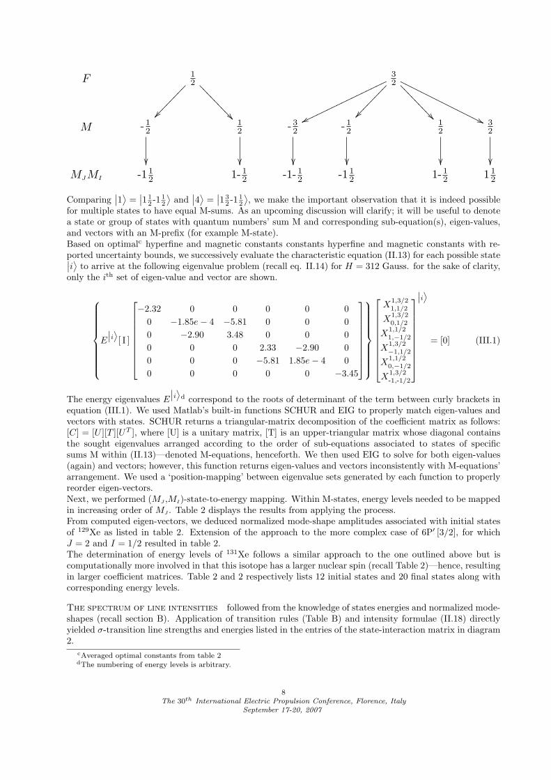
, we start by determining all allowed values for F, MJ ,and MI using (II.1), (II.12a), and (II.12b), respectively. The scheme is shown in table (2).

F MJ MJ

12

52 -1 0 1 - 1

212

Table 4. Possible F , MJ , and MIvalues for 6S′ [1/2] state

To each F -number is associated a corresponding set of sums M given by (II.2); which, in turn, providesmeans for coupling MJ and MI to form a particular state

∣

∣JFMJMI

⟩

(see equation (II.2)). The simple

process (summarized below) reveals six possible states for 6S′ [1/2] (∣

∣i⟩

, i = 1 . . . 6 - labels are respectivelyassociated to states starting from left to right in the diagram below).



F 12

��>>

>>>>

>>>

��

��

32

wwnnnnnnnnnnnnnnnnn

��

��

��>>

>>>>

>>>

''OOOOOOOOOOOOOOOO

M - 12

��

12

��

- 32

��

- 12

��

12

��

32

��

MJMI -1 12 1- 1

2 -1- 12 -1 1

2 1- 12 1 1

2

Comparing∣

∣1⟩

=∣

∣1 12 -1 1

2

⟩

and∣

∣4⟩

=∣

∣1 32 -1 1

2

⟩

, we make the important observation that it is indeed possiblefor multiple states to have equal M-sums. As an upcoming discussion will clarify; it will be useful to denotea state or group of states with quantum numbers’ sum M and corresponding sub-equation(s), eigen-values,and vectors with an M-prefix (for example M-state).Based on optimalc hyperfine and magnetic constants constants hyperfine and magnetic constants with re-ported uncertainty bounds, we successively evaluate the characteristic equation (II.13) for each possible state∣

∣i⟩

to arrive at the following eigenvalue problem (recall eq. II.14) for H = 312 Gauss. for the sake of clarity,only the ith set of eigen-value and vector are shown.

E

∣

∣i⟩

[ I ]

−2.32 0 0 0 0 0

0 −1.85e − 4 −5.81 0 0 0

0 −2.90 3.48 0 0 0

0 0 0 2.33 −2.90 0

0 0 0 −5.81 1.85e − 4 0

0 0 0 0 0 −3.45

X1,3/21,1/2

X1,3/20,1/2

X1,1/21,−1/2

X1,3/2−1,1/2

X1,1/20,−1/2

X1,3/2-1,-1/2

∣

∣i⟩

= [0] (III.1)

The energy eigenvalues E

∣

∣i⟩

d correspond to the roots of determinant of the term between curly brackets inequation (III.1). We used Matlab’s built-in functions SCHUR and EIG to properly match eigen-values andvectors with states. SCHUR returns a triangular-matrix decomposition of the coefficient matrix as follows:[C] = [U ][T ][UT ], where [U] is a unitary matrix, [T] is an upper-triangular matrix whose diagonal containsthe sought eigenvalues arranged according to the order of sub-equations associated to states of specificsums M within (II.13)—denoted M-equations, henceforth. We then used EIG to solve for both eigen-values(again) and vectors; however, this function returns eigen-values and vectors inconsistently with M-equations’arrangement. We used a ‘position-mapping’ between eigenvalue sets generated by each function to properlyreorder eigen-vectors.Next, we performed (MJ ,MI)-state-to-energy mapping. Within M-states, energy levels needed to be mappedin increasing order of MJ . Table 2 displays the results from applying the process.From computed eigen-vectors, we deduced normalized mode-shape amplitudes associated with initial statesof 129Xe as listed in table 2. Extension of the approach to the more complex case of 6P′ [3/2], for whichJ = 2 and I = 1/2 resulted in table 2.The determination of energy levels of 131Xe follows a similar approach to the one outlined above but iscomputationally more involved in that this isotope has a larger nuclear spin (recall Table 2)—hence, resultingin larger coefficient matrices. Table 2 and 2 respectively lists 12 initial states and 20 final states along withcorresponding energy levels.

The spectrum of line intensities followed from the knowledge of states energies and normalized mode-shapes (recall section B). Application of transition rules (Table B) and intensity formulae (II.18) directlyyielded σ-transition line strengths and energies listed in the entries of the state-interaction matrix in diagram2.

cAveraged optimal constants from table 2dThe numbering of energy levels is arbitrary.



Mass Number 129 131 Ref.

I 12

32

6

µN [(mp

me)−1] -0.7768(0.0001) 0.700(0.05) ?

A [GHz]-5801.1(12.8) 1713.7(6) 17

-2892.4(6.9) 858.9(3.1) 8

gJ

1.321 1.321 13

1.190(0.001) 1.190(0.001) 2

Table 5. Physical parameters associated with stable isotopes 129Xe and 131Xe having hyperfine structure.Upper and lower sub-rows are respectively associated with initial and final states. From µN and I, we deducedLande-gIfactor using: gI = (

mp

me)−1 µN

I, where the proton-to-electron mass ratio

mp

me= 1836. The numbers

between parentheses are uncertainty widths (e.g. 1.190(0.001) is equivalent to 1.190 ± 0.001) that, in somecases, incorporate widths by other authors cited within listed sources.

StateEnergy Mode-shape amplitudes

[GHz] X1,3/21,1/2 X

1,3/20,1/2 X

1,1/21,-1/2 X

1,3/2-1,1/2 X

1,1/20,-1/2 X

1,3/2-1,-1/2

∣

∣1 321 1

2

⟩

-2.33 0.707 - - - - -∣

∣1 320 1

2

⟩

-2.72 - -0.834 0.552 - - -∣

∣1 121- 1

2

⟩

6.20 - -0.390 -0.590 - - -∣

∣1 32 -1 1

2

⟩

-3.10 - - - 0.426 0.564 -∣

∣1 120- 1

2

⟩

5.43 - - - 0.798 -0.603 -∣

∣1 32 -1- 1

2

⟩

-3.50 - - - - - 0.577

Table 6. 129Xe upper state’s (6S′ [1/2]) energy levels along with corresponding mode-shape amplitudes

Sta

te

∣ ∣

25 22

1 2

⟩

∣ ∣

25 21

1 2

⟩

∣ ∣

23 22-

1 2

⟩

∣ ∣

25 20

1 2

⟩

∣ ∣

23 21-

1 2

⟩

∣ ∣

25 2-1

1 2

⟩

∣ ∣

23 20-

1 2

⟩

∣ ∣

25 2-2

1 2

⟩

∣ ∣

23 2-1

-1 2

⟩

∣ ∣

25 2-2

-1 2

⟩

Lab

el

∣ ∣

1⟩

∣ ∣

2⟩

∣ ∣

3⟩

∣ ∣

4⟩

∣ ∣

5⟩

∣ ∣

6⟩

∣ ∣

7⟩

∣ ∣

8⟩

∣ ∣

9⟩

∣ ∣

10⟩

Energy (GHz) -1.85 -2.28 -5.28 -2.69 4.66 -3.11 4.04 -3.52 3.41 -3.93

Table 7. 129Xe final state’s (6P′ [3/2]) energy levels

Sta

te

∣ ∣

15 21

3 2

⟩

∣ ∣

15 20

3 2

⟩

∣ ∣

13 21

1 2

⟩

∣ ∣

15 2-1

3 2

⟩

∣ ∣

13 20

1 2

⟩

∣ ∣

11 21-

1 2

⟩

∣ ∣

15 2-1

1 2

⟩

∣ ∣

13 20-

1 2

⟩

∣ ∣

11 21-

3 2

⟩

∣ ∣

15 2-1

-1 2

⟩

∣ ∣

13 20-

3 2

⟩

∣ ∣

15 2-1

-3 2

⟩

Lab

el

∣ ∣

1⟩

∣ ∣

2⟩

∣ ∣

3⟩

∣ ∣

4⟩

∣ ∣

5⟩

∣ ∣

6⟩

∣ ∣

7⟩

∣ ∣

8⟩

∣ ∣

9⟩

∣ ∣

10⟩

∣ ∣

11⟩

∣ ∣

12⟩

Energy (GHz) 3.15 -1.50 2.94 -4.55 -1.60 2.72 -4.18 -1.75 2.49 -1.97 2.25 2.00

Table 8. 131Xe initial state’s (6S′ [1/2]) energy levels



Sta

te

∣ ∣

27 22

3 2

⟩

∣ ∣

27 21

3 2

⟩

∣ ∣

25 22

1 2

⟩

∣ ∣

27 20

3 2

⟩

∣ ∣

25 21

1 2

⟩

∣ ∣

23 22-

1 2

⟩

∣ ∣

27 2-1

3 2

⟩

∣ ∣

25 20

1 2

⟩

∣ ∣

23 21-

1 2

⟩

∣ ∣

21 22-

3 2

⟩

∣ ∣

27 2-2

3 2

⟩

∣ ∣

25 2-1

1 2

⟩

∣ ∣

23 20-

1 2

⟩

∣ ∣

21 21-

3 2

⟩

∣ ∣

27 2-2

1 2

⟩

∣ ∣

25 2-1

-1 2

⟩

∣ ∣

23 20-

3 2

⟩

∣ ∣

27 2-2

-1 2

⟩

∣ ∣

25 2-1

-3 2

⟩

∣ ∣

27 2-2

-3 2

⟩

Lab

el

∣ ∣

1⟩

∣ ∣

2⟩

∣ ∣

3⟩

∣ ∣

4⟩

∣ ∣

5⟩

∣ ∣

6⟩

∣ ∣

7⟩

∣ ∣

8⟩

∣ ∣

9⟩

∣ ∣

10⟩

∣ ∣

11⟩

∣ ∣

12⟩

∣ ∣

13⟩

∣ ∣

14⟩

∣ ∣

15⟩

∣ ∣

16⟩

∣ ∣

17⟩

∣ ∣

18⟩

∣ ∣

19⟩

∣ ∣

20⟩

Energy (GHz) 3.60 0.364 3.33 -2.02 0.0970 3.05 -3.57 -2.23 -0.201 2.76 -4.53 -2.72 -0.532 2.46 -3.25 -0.888 2.16 -1.27 1.85 1.53

Table 9. 131Xe final state’s (6P′ [3/2]) energy levels

∣ ∣

1⟩

∣ ∣

2⟩

∣ ∣

3⟩

∣ ∣

4⟩

∣ ∣

5⟩

∣ ∣

6⟩

∣ ∣

7⟩

∣ ∣

8⟩

∣ ∣

9⟩

∣ ∣

10⟩

⟨

1∣

∣ (-0.37,7.6) (6.2,0.82) - - (0.20,3.3) (7.8,1.1) - - - -⟨

2∣

∣ (-8.7,0.0025) (-2.2,9.6) - - (-8.2,0.00043) (-0.55,3.6) - - - -⟨

3∣

∣ - - (0.40,6.9) (8.5,0.73) - - (-0.21,4.0) (6.9,0.95) - -⟨

4∣

∣ - - (-8.8,0.00085) (-0.74,10) - - (-9.4,0.0011) (-2.3,3.1) - -⟨

5∣

∣ - - - - (-0.076,2) (7.5,2) - - (0.56,12) -⟨

6∣

∣ - - - - - - (-0.020,2) (7.1,2) - (-0.55,12)

Table 10. Energies(GHz) and normalized intensities of σ-transition lines in 129Xe: 6S′ [1/2]→ 6P′ [3/2]

Applying the above approach to 131Xe, reveals 74 σ-transitions. The overlaid spectrum in figure 2 illustratesthe shifting due to each isotope. Furthermore, the normalized line intensities have been scaled to accountfor relative natural abundances. Table 2 provides shifts and percent abundances associated of each isotope.Figure 2 showing σ− transitions completes the spectrum of lines.

Masse number 129 131

Shift [MHz] 213.4(4.7) 189.7(6.1)

Abundance [%] 26.4 21.2

Table 11. Isotope energy shifts17 and natural abundances6 of stable xenon species with non-zero nuclear spin

Broadening of lines To simulate the warm spectrum W (ν) or absorption spectrum of xenon atoms inthe plasma environment, we apply a Voigt profile7 to the spectrum of transition lines Y (ν); such a profileaccounts for two predominant physical phenomena: the Heisenberg Uncertainty Principle (HUP) and thethermal motion of particles—assumed to be at equilibrium. As expressed in (III.2), the profile results fromthe convolution of a cold spectrum C (ν) with a maxwellian distribution.15

W (ν) = C (ν) ⊗ D (ν) , where (III.2)

D (ν) = exp

[

M

2kT(λo ν)

2

]

(III.3)

The HUP enters in the picture through C, which results from Lorentz broadening. As expressed in (III.4),the effect is simulated by convolving Y with a Lorentzian lineshape L (ν) defined in (III.5).

C (ν) = L (ν) ⊗ Y (ν) , where (III.4)

L (ν) =

n∑

i

1

π

∆ν

(ν − νi)2

+ (∆ν)2 , where (III.5)

the summation in (III.5) accounts for all lines (numbered i = 1, 2, . . . , n) and ∆ν =Aij

2π is the width ofindividual lines at half-maximum. Figure 2 respectively illustrate how Lorentizian and Doppler broadeninglead to the sought Voigt profile. We set Aij to 8.81106sec−1 based on a reported value of 6.36106sec−1

(uncertainty ±40%)e (see C).11

eoptimal physical parameters are all within bounds of uncertainties reported by their authors and were found based on abest fit of the non-linear least-squares approach discussed in C



−8 −6 −4 −2 0 2 4 60

0.5

1

1.5

2

2.5

3


NO

RM

ALI

ZE

D T

RA

NS

ITIO

N IN

TE

NS

ITIE

S[%

nat

ural

abu

ndan

ce s

calin

g]

129Xe: 26.4 %, ∆ν = 209 MHz131Xe: 21.2 %, ∆ν = 184 MHz

−8 −6 −4 −2 0 2 4 60

0.5

1

1.5

2

2.5

3

3.5

4


NO

RM

ALI

ZE

D T

RA

NS

ITIO

N IN

TE

NS

ITIE

Sna

tura

l abu

ndan

ce s

calin

g (%

)

129Xe: 131Xe:

Figure 2. σ− and σ+ transition line strengths of 129Xe and131Xe. Unshifted lines appear dashed.

−5 −4 −3 −2 −1 0 1 2 3 4 50

0.1

0.2

0.3

0.4

0.5

0.6

0.7


NO

RM

ALI

ZE

D S

PE

CT

RA

Transition linesCold plasmaWarm plasma

Figure 3. Illustration of Voigt profile generation from the spectrum of transition lines. The cold and warmspectra shown are based on Lorentz and Doppler broadenings of transition lines. H = 300 Gauss in this plot



IV. Validation of the computational model

A. Experimental setup

We used spectral data from a galvatron to validate the non-linear Zeeman-HFS model. A detailed descrip-tion of the experiment—performed at the University of Michigan’s (UM) Plasma dynamics and ElectricPropulsion Laboratory (PEPL)—can be found in.16 The simple device consists of a glass tube filled withxenon and argon (non-reacting filler) bottle. It encloses two electrodes for plasma breakdown. The galva-tron is calibrated such that when the plasma is exited by a light source tuned to a particular transition’swavelength, its voltage output varies proportionally with the radiative intensity of the gas absorption. Theexciting light source consists of a tunable single-mode diode-laser centered at 834.682 nm (air-wavelengthof the 6S′ [1/2] → 6P′ [3/2] transition). Scans spanned 10 GHz mode-hop-free frequency detuning ranges.A 2 GHz free-spectral-range (FSR) Fabry-Perot interferometer accurate to 6.7 MHz insured high-resolutiondetuning. A pair of Helmholtz coils was placed on either side of the galvatron so that their symmetry axis isperpendicular to the galvatron’s axis. The error on field strength measurements was estimated at 2%. Thisarrangement permitted the generation of a variable external field of maximal strength along the path of thelaser, which stimulated the optogalvanic effect as it propagated through the cylindrical electrodes within thespread of the plasma. To excite π or σ-transitions, the laser was polarized in front of the galvatron’s inputaperture. A lock-in amplifier operating with a time-constant of 300 ms read output voltages and relayedthem to a PC; the latter controlled the voltage of the laser’s piezo-electric tuning element over 10 Volt-spanramp.

B. Continuity of transition energies and and smooth distribution of absorption spectra

As mentioned in B, the non-linear Zeeman-hyperfine model is, in theory, applicable to an arbitrarily widerange of field strengths—machine tolerance being the only constraint, the range extends from 0.01 to 50,000Gauss. For the purpose of investigating field strengths in electric thrusters, this limitation poses no problemsince typical field strengths fall well within that range (0 to 200 gauss).12 Figures B and B, respectively,illustrate continuous variations of transition energies from 0.01 to 1000 Gauss for 129Xe and 131Xe. Becausethe energies resulting from the characteristic equation (equation (II.13)) denote shift with respect to somehypothetical level (1), we had to shift transition energies about the center of gravity of the lines; that is,transition energies were weighted with respected to corresponding intensities.Energy level continuity led to smooth variations of cold and warm spectra with magnetic field intensity.Figure B illustrates this through a surface plot of Xe I cold spectrum about 834.682 nm.

C. Solving for the magnetic field strength and plasma temperature using a non-linear least-

squares method

Description of the non-linear least-squares solver We applied Matlab’s built-in function LSQNON-LIN to our optimization problem. It finds optimal design paramaters p

∗ = p∗(p∗1, p

∗2, . . . p

∗

k . . . p∗n) that min-imize a smooth non-linear function of the type ǫ(p) = 1

2

∑

i(Ti(p) − Ei)2 while parameters are constrained

within closed-bound intervals. Starting with a guessed set of parameters po = p

o(po1, p

o2, . . . p

ok . . . po

n), themethod allows the progression of ǫ(p) towards the minimum ǫ(p∗) of the error function by iterative stepsof optimal lengths along steepest descent search directions corresponding to ∇ǫ at Iterative points towardsthe point of convergence. Convergence of the solver to an optimal point or solution is achieved when thechange in the norm of the residualf falls below a tolerance level. This novel non-linear method,3 which suitedfor large scale problems of many variables is more efficient than traditional linear optimization techniquesin its interior-reflective Newton line-search technique that allows a quadratic decay in the residual normand insures global minimization of the error function. The efficiency stems primarily from the fact thatp progresses towards p∗ along a feasible region—the bounded path, along which p progresses g. An affinetransformation of the vector space defined by pk(k = 1, 2, . . . , n) and successive reflections of steepest descentdirections with respect to prior ones about the normal of the feasible region at each point (in a piece-wisefashion) generates a search path that remains well centered between the boudaries—key to fast and robust

fthe residual, which is not to be confused with the error between fit and experiment, is related to the gradient of the errorfunction at some point of the iteration path leading to the point of convergence

gThe interior-reflective Newton method deviates from lesser efficient traditional methods like the Simplex method whichcauses a marching of pm along the boundaries3



−10 −8 −6 −4 −2 0 2 4 6 8 10

200

400

600

800

1000

1200

TRANSITION ENERGIES [GHz]

MA

GN

ET

IC F

IELD

ST

RE

NG

TH

[Gau

ss]

Isotope: 129Xe

−10 −8 −6 −4 −2 0 2 4 6 8 10

200

400

600

800

1000

1200

TRANSITION ENERGIES [GHz]

MA

GN

ET

IC F

IELD

ST

RE

NG

TH

[Gau

ss]

Isotope: 131Xe

Figure 4. Variation of transition energies of 129Xe and131Xe with magnetic field strength



Figure 5. Smooth surface distribution of cold spectra with respect to magnetic field intensity

convergence.

We determined optimal physical parameters and target solutions as a preamble to solving forthe external magnetic field intensity and plasma kinetic temperature from remote initial guesses. Becausemere use of po would not necessarily yield the best predictions on galvatron’s plasma temperature and theexternal field strength, we solved for the optimal variables within their respective uncertainty bounds. Wealso determined target external magnetic field intensities and plasma kinetic temperatures. By ‘target’, wemean our best estimates of experimental settings within reported uncertainty bounds.We treated all unknown parameters as components of a vector p bounded within

p ∈ [pmin, po[⋃

]po, pmax],

where po denotes a vector of error interval centers reported in tables 2, 1, and 2. We set the tolerance of thesolver to 10−7 to match the resolution of the galvatron’s voltage measurements and frequency detuning h.and that of the frequency detuning i.We used LSQNONLIN to solve for p

∗ listed in table C at field strength intensities spanning 30 to 300 gauss.The table also lists averages p∗ (right-end of table) and relative deviations of error functions (bottom-end

of table) ∆∗ǫ = ǫ∗−ǫo

ǫoand ∆ǫ∗ = ǫ∗−ǫo

ǫo. At all field strength settings, a reduction of the error function is

evident. From table C, we also make the important observation that ∆ǫ∗ ≈ ∆ǫ∗ ; A priori, this promptsus to consistently use p∗ as optimal input physical parameters to the temperature and field-strength solverfor fitting any σ-spectral distribution excited by an arbitrary external field of strength falling within theinvestigated range [30, 300].In addition to the physical parameters mentionned above, optimal field intensities were simultaneously com-puted within some 100% error interval, which we set wide in the hope to account for experimental errors(see section A) and any shifts from interactions between plasma-induced and the external magnetic field.

hThe precision level of spectral intensity measurements was 10−7 V and was limited by the lock-in amplifier’s sensivity ormaximum bits sent to the PC

iThe resolution on frequency detuning of 6.710−3 GHz (recall A) translates to 2.010−7cm−1



Table C reports the resulting effective (or ‘target’) field intensities corresponding to each particular set ofparameters at the various Bexp settings j included for comparison. We treated the computed optimal values,not measured external field intensities, as target values for the B and T solver—described and validated insection C. We note that target field intensities are better matches to measured center values as the latterincrease. The 120-Gauss setting separates a group of poorer from better matches.

jrecall that Bexp corresponds to measured maximal strengths along the center axis of the current-carrying coils



Magnetic field strengths (Gauss)

Center 33.19 65.6 99.01 131.9 164.8 197.8 230.8 263.7 296.7 329.7 329.7

Optimal 16.59 32.87 49.51 112.4 142.6 168.7 210.9 236.3 272.3 311.3 311.3

States Isotopes Optimal variables averages

Galvatron temperatures (K)

450 462.7 512.2 467.7 450.1 450.8 471.8 452.3 450 504.4 467.2

Isotope shifts (MHz) - relative to 136

124 250.2 250.2 250.2 250.3 250.2 250.2 250.2 250.2 250.2 250.2 250.2

126 209.1 209.1 209.1 209.1 209.1 209.1 209.1 209.1 209.1 209.1 209.1

128 167.9 167.9 167.9 167.9 167.9 167.9 167.9 167.9 167.9 167.9 167.9

129 208.7 208.7 208.7 208.7 208.7 208.7 208.7 208.7 208.7 208.7 208.7

130 130.4 130.4 130.4 130.4 130.4 130.4 130.4 130.4 130.4 130.4 130.4

131 183.6 183.6 183.6 183.6 183.6 183.6 183.6 183.6 183.6 183.6 183.6

132 98.9 98.9 98.9 98.91 98.9 98.9 98.9 98.9 98.9 98.9 98.9

134 62.9 62.9 62.9 62.9 62.9 62.9 62.9 62.9 62.9 62.9 62.9

Hyperfine constants (MHz)

6S′ [1/2]129 -5811 -5811 -5786 -5811 -5786 -5786 -5804 -5786 -5811 -5811 -5801

131 -2888 -2898 -2899 -2899 -2899 -2899 -2899 -2899 -2888 -2896 -2897

6P′ [3/2]129 1718 1718 1718 1718 1718 1718 1718 1718 1718 1718 1718

131 855.8 855.8 855.8 855.8 855.8 855.8 855.8 855.8 855.8 855.8 855.8

Electron Lande-g factors: gJ

6S′ [1/2] 1.321 1.321 1.321 1.321 1.321 1.321 1.321 1.321 1.321 1.321 1.321

6P′ [3/2] 1.189 1.189 1.189 1.189 1.189 1.19 1.189 1.189 1.189 1.191 1.189

Nuclear moments: µN

129 -0.7769 -0.7767 -0.7767 -0.7767 -0.7767 -0.7767 -0.7767 -0.7767 -0.7769 -0.7769 -0.7768

131 0.6498 0.6498 0.6498 0.7498 0.7498 0.7498 0.7498 0.7498 0.7498 0.7498 0.7198

Einstein emission coefficient

0.7997 0.8903 0.8904 0.8904 0.8904 0.89 0.8904 0.8904 0.8897 0.8904 0.8812

Percent relative error from center

-107.6 -96.02 -115 -158.9 -218.3 -266.4 -240.1 -336.4 -353 -229.1 -193.2

Table 12. Determination of Optimal Physical Parameters for Input in Temperature and Field Strength Solver



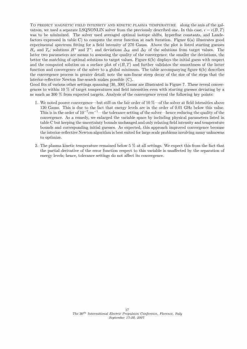
To predict magnetic field intensity and kinetic plasma temperature along the axis of the gal-vatron, we used a separate LSQNONLIN solver from the previously described one. In this case, ǫ = ǫ(B, T )was to be minimized. The solver used averaged optimal isotope shifts, hyperfine constants, and Lande-factors expressed in table C) to compute the error function at each iteration. Figure 6(a) illustrates goodexperimental spectrum fitting for a field intensity of 270 Gauss. Above the plot is listed starting guessesHo and To; solutions H∗ and T ∗; and deviations ∆H and ∆T of the solutions from target values. Thelatter two parameters are means to assessing the quality of the convergence; the smaller the deviations, thebetter the matching of optimal solutions to target values. Figure 6(b) displays the initial guess with respectand the computed solution on a surface plot of ǫ(B, T ) and further validates the smoothness of the latterfunction and convergence of the solver to a global minimum. The table accompanying figure 6(b) describesthe convergence process in greater detail; note the non-linear steep decay of the size of the steps that theinterior-reflective Newton line-search makes possible (C).Good fits of various other settings spanning [30, 300] Gauss are illustrated in Figure 7. These reveal conver-gences to within 10 % of target temperatures and field intensities even with starting guesses deviating by aas much as 300 % from expected targets. Analysis of the convergence reveal the following key points:

1. We noted poorer convergence—but still on the fair order of 10 %—of the solver at field intensities above120 Gauss. This is due to the fact that energy levels are in the order of 0.01 GHz below this value.This is in the order of 10−7cm−1—the tolerance setting of the solver—hence reducing the quality of theconvergence. As a remedy, we enlarged the variable space by including physical parameters listed intable C but keeping the uncertainty bounds unchanged and only relaxing field intensity and temperaturebounds and corresponding initial guesses. As expected, this approach improved convergence becausethe interior-reflective Newton algorithm is best suited for large scale problems involving many unknownsto optimize.

2. The plasma kinetic temperature remained below 5 % at all settings. We expect this from the fact thatthe partial derivative of the error function respect to this variable is unaffected by the separation ofenergy levels; hence, tolerance settings do not affect its convergence.



−5 −4 −3 −2 −1 0 1 2 3 4 5

0.05

0.1

0.15

0.2

0.25

0.3

0.35

0.4

0.45

0.5

FREQUENCY DETUNING (GHz)

NO

RM

ALI

ZE

D S

PE

CT

RA

[Bo, B*(∆B)] = [517, 273(0%)] Gauss [To, T*(∆

T)] = [700, 467(4%)] K.

Z−HFS ModelExperiment

(a) Variation of fitting-error with B and T

(b) Spectral fitting for optimal B and T

Iteration ǫ(B, T ) Norm of step

1 0.175723 1

2 0.053548 6.86105

3 0.0479 2.9966

4 0.0476004 0.82513

5 0.047596 0.104012

Figure 6. Computation of the external magnetic field intensity and plasma kinetic temperature in an opto-galvanic cell based non-linear least-squares fitting of the Xe I absorption σ-spectrum at 834.682 nm (in air)for a field setting of 270 Gauss



−5 −4 −3 −2 −1 0 1 2 3 4 5

0.1

0.2

0.3

0.4

0.5

0.6

0.7

0.8

0.9


NO

RM

ALI

ZE

D S

PE

CT

RA

[Bo, B*(∆B)] = [43, 15(−8%)] Gauss [To, T*(∆

T)] = [700, 430(−5%)] K.


(a) 30 Gauss

−5 −4 −3 −2 −1 0 1 2 3 4 5

0.1

0.2

0.3

0.4

0.5

0.6

0.7

0.8

0.9


NO

RM

ALI

ZE

D S

PE

CT

RA

[Bo, B*(∆B)] = [85, 30(−10%)] Gauss [To, T*(∆

T)] = [700, 468(1%)] K.


(b) 60 Gauss

−5 −4 −3 −2 −1 0 1 2 3 4 5

0.1

0.2

0.3

0.4

0.5

0.6

0.7


NO

RM

ALI

ZE

D S

PE

CT

RA

[Bo, B*(∆B)] = [171, 113(1%)] Gauss [To, T*(∆

T)] = [700, 459(−2%)] K.


(c) 120 Gauss

−5 −4 −3 −2 −1 0 1 2 3 4 50

0.1

0.2

0.3

0.4

0.5

0.6


NO

RM

ALI

ZE

D S

PE

CT

RA

[Bo, B*(∆B)] = [320, 170(1%)] Gauss [To, T*(∆

T)] = [700, 419(−8%)] K.


(d) 180 Gauss

−5 −4 −3 −2 −1 0 1 2 3 4 5

0.05

0.1

0.15

0.2

0.25

0.3

0.35

0.4

0.45

0.5


NO

RM

ALI

ZE

D S

PE

CT

RA

[Bo, B*(∆B)] = [449, 236(−0%)] Gauss [To, T*(∆

T)] = [700, 443(−2%)] K.


(e) 240 Gauss

−5 −4 −3 −2 −1 0 1 2 3 4 5

0.05

0.1

0.15

0.2

0.25

0.3

0.35

0.4

0.45


NO

RM

ALI

ZE

D S

PE

CT

RA

[Bo, B*(∆B)] = [591, 313(0%)] Gauss [To, T*(∆

T)] = [700, 519(3%)] K.


(f) 300 Gauss

Figure 7. Least-squares fitting of neutral xenon absorption spectra at 834.682 nm in an opto-galvanic cell atvarious external magnetic field intensity settings. The fitting is based on optimal magnetic field intensity andplasma kinetic temperature outputted by Matlab’s LSQNONLIN solver.



Sensitivity of solver to signal-to-noise ratio Though the above analysis dealt with opto-galvanicspectra, we stress that the main goal of the solver is to resolve magnetic field intensities and kinetic tempera-tures from laser-induced fluorescence spectra measured in electric thruster discharges. The latter spectra aretypically much noisier with signal-to-noise (SNR) ratios on the order of 100.14 Hence, to further validate ofthe B and T solver, we studied the effect of gaussian noise addition to experimental spectra on convergence.We found little impact of random artificial noise on the quality of convergence at SNR > 200. And in somecases it actually, improved convergence. At high field intensity settings B-convergence remained good asillustrated in the fit of figure 8(a) at 30 Gauss despite the effect of tolerance setting on its convergence. Atlower settings, however, convergence was poorer. The quality of convergence is better assessed from figures8(b) and 8(c) showing the evolution of the devations of optimal variables from their corresponding targetvalues with SNR. Gaussian noise had little effect on the convergence at SNRs above 200. And in someextreme cases such as the 30 Gauss setting shown on 8(a) at an SNR of 20, gaussian noise actually seems tohelp convergence; the quadratic nature of the error-function which relates it to the gaussian distribution ofthe random noise may be at the origin of this anomaly.



−5 −4 −3 −2 −1 0 1 2 3 4 5

−0.6

−0.4

−0.2

0

0.2

0.4

0.6

0.8

1

1.2

1.4


NO

RM

ALI

ZE

D S

PE

CT

RA

SNR = 25 [Ho, H*(∆H)] = [7, 21(20%)] Gauss [To, T*(∆T)] = [700, 417(−8%)] K.


(a) Illustration of noisy spectrum fitting

100

101

102

103

104

−100

−80

−60

−40

−20

0

20

40

60

80

30

60

90

150180

210

300

SIGNAL−T0−NOISE RATIO

∆ Ho [

%]

(b) Effect of SNR on B convergence

100

101

102

103

104

−40

−30

−20

−10

0

10

20

30

40

50

60

30

6090

150

180

210

300

SIGNAL−T0−NOISE RATIO

∆ T* [%

]

(c) Effect of SNR on T convergence

Figure 8. Effect of signal-to-noise ratio (SNR) on the optimization of external magnetic field intensity (B)and plasma kinetic temperature (T) of an opto-galvanic cell based on non-linear least-squares fitting of neutralxenon absorption spectra at 834.682 nm (in air)



V. conclusion

The non-linear Zeeman effect on the hyperfine structure is to-date the most accurate theory for modelingof hydrogen-like atomic spectra. We successfully used it to model neutral xenon absorption spectra in theplasma environment produced within an opto-galvanic cell to which an external magnetic field was applied.The reliability of the model prompted us to use it at a input function to a non-linear solver of magneticintensity and kinetic plasma kinetic temperature based on best experimental spectra fitting. We noted goodconvergence of the solver in both variables even in the presence of Gaussian noise, provided the signal-to-noise ratio (SNR) remained above 200. At lower SNRs, errors on optimal values with respect to expectedtarget solutions still remained below 80 %. Overall, we noted similar convergence of kinetic temperatureat all field intensities investigated, but differing convergence behaviors for magnetic field intensities; for thelatter variable, we noted poorer convergence at low field settings. The results found in this study makeour non-linear solver a good computational tool for the study of the interaction between external magneticfield and xenon Hall thruster discharges as well as for thermal speed extraction from LIF spectra. Moreimportantly, we project a trivial extension of the method to multiply-ionized xenon species, whose studymay shed greater light on thruster-life limiting phenomena such as acceleration-grid and cathode erosions.

References

1R. F Bacher. The Zeeman Effect of Hyperfine Structure. PhD thesis, University of Michigan, Ann Arbor, MI, 1930.2D. A. Bethe and R. R. Bacher. Nuclear physics a. stationary states of nuclei. Review of Modern Physics, 8, 1936.3T. F. Coleman and Y. Li. On the convergence of interior-reflective newton methods for nonlinear minimization subject to

bounds, 1994.4C.G. Darwin. The zeeman effect and spherical harmonics. volume 115 of Proceedings of the Royal Society of London. Series

A, pages 1–19, 1927.5K. Darwin. Examples of the zeeman effect at intermediate strengths of magnetic field. volume 118 of Proceedings of the

Royal Society of London. Series A, pages 264–285, 1928.6R. B. Firestone. Table of Isotopes. Wiley, New York, 1999.7H. Haken and H. C. Wolf. The Physics of Atoms and Quanta. Springer, Verlag Berlin Heidelberg, 7th edition, 1997.8D. A. Jackson and M. C. Coulombe. Hyperfine structure in the arc spectrum of xenon. volume 327 of Proceedings of the

Royal Society of London. Series A, Mathematical and Physical Sciences, pages 137–145, 1972.9W. H. King. Isotope Shifts in Atomic Spectra. Plenum Press, New York, 1984.

10E. Merzbacher. Quantum Mechanics. Wiley, New York, 3rd edition, 1997.11M. H. Miller, R. A. Roig, and R. D. Bengtson. Transition probabilities of xe i and xe ii. Physical Review A, 8(1), 1973.12P. Y. Peterson, A. D. Gallimore, and J. M. Haas. Experimental investigation of a hall thruster internal magnetic fieldtopography. 27th International Electric Propulsion Conference, Pasadena, CA, 2001.13E. B. Saloman. Energy levels and observed spectral lines of xenon, xe i through xe liv. Technical report, National Instituteof Standards and Technology, Gaithersburg, Maryland 20899-8422, 2004.14T. B. Smith. Deconvolution of Ion Velocity Distributions from Laser-Induced Fluorescence Spectra of Xenon Electrostatic

Thruster Plumes. PhD thesis, University of Michigan, Ann Arbor, MI, 2003.15T. B. Smith, D. A. Herman, A. D. Gallimore, and R. P. Drake. Deconvolution of axial velocity distributions from hall thrusterlif spectra. 27th International Electric Propulsion Conference, Pasadena, CA, 2001.16T. B. Smith, W. Huang, B. B. Ngom, and A. D. Gallimore. Optogalvanic and absorption spectroscopy of the zeeman effectin xenon. 30th International Electric Propulsion Conference, Florence, Italy, 2007.17M. Suzuki, K. Katoh, and N. Nishimiya. Saturated absorption spectroscopy of xe using a gaas semiconductor laser. Spec-

trochimica Acta Part A, 58:2519–2531, 2002.



numerical simulation of the zeeman eﬀect from laser...

Documents