numerical simulation of wave propagation in media with ... · numerical simulation of wave...

$: Numerical simulation of wave propagation in media with ... · Numerical simulation of wave propagation in media with discrete distributions of fractures: effects of fracture sizes$
January 27, 2003 13:49 Geophysical Journal International gji˙1876

Geophys. J. Int. (2003) 152, 649–668

Numerical simulation of wave propagation in media with discretedistributions of fractures: effects of fracture sizesand spatial distributions

S. Vlastos,1,2 E. Liu,1 I. G. Main2 and X.-Y. Li11British Geological Survey, Murchison House, West Mains Road, Edinburgh EH9 3LA, UK. E-mail: [email protected] of Geology and Geophysics, University of Edinburgh, Grant Institute, West Mains Road, Edinburgh EH9 3JW, UK

Accepted 2002 September 11. Received 2002 September 6; in original form 2002 May 25

S U M M A R YWe model seismic wave propagation in media with discrete distributions of fractures using thepseudospectral method. The implementation of fractures with a vanishing width in the 2-Dfinite-difference grids is done using an effective medium theory (that is, the Coates and Schoen-berg method). Fractures are treated as highly compliant interfaces inside a solid rock mass.For the physical representation of the fractures the concept of linear slip deformation or thedisplacement discontinuity method is used. According to this model, the effective complianceof a rock mass with one or several fracture sets can be found as the sum of the compliancesof the host (background) rock and those of all the fractures. To first order, the backgroundrock and fracture parameters can be related to the effective anisotropic coefficients, whichgovern the influence of anisotropy on various seismic signatures. We test the validity of themethod and examine the accuracy of the synthetic seismograms by a comparison with theo-retical ray traveltimes. We present three numerical examples to show the effects of differentfracture distributions. The first example shows that different spatial distributions of the samefractures produce different wavefield characteristics. The second example examines the effectsof variation of fracture scale length (size) compared with the wavelength. The final exampleexamines the case of fractures with a power-law (fractal) distribution of sizes and shows howthat affects the wavefield propagation in fractured rock. We conclude that characterization offractured rock based on the concept of seismic anisotropy using effective medium theoriesmust be used with caution. Scale length and the spatial distributions of fractures, which arenot properly treated in such theories, have a strong influence on the characteristics of wavepropagation.

Key words: cracked media, effective medium theory, fractures, finite-difference methods,wave propagation.

1 I N T R O D U C T I O N

Numerical modelling techniques are now becoming very commonfor understanding the complicated nature of seismic wave propa-gation in fractured rocks. The scientific community has shown anincreasing interest in this subject, and currently there are a vari-ety of approaches for forward modelling. Analytic expressions forthe description of elastic wave propagation in the presence of frac-tures are only available for rather simple cases, that is, single crackswith simple geometries (Mal 1970), and in most cases are onlyvalid in the far field (Liu et al. 1997). In complex situations, so-lutions based on Born or Rytov approximations may be used (Wu& Aki 1985). These approximations become accurate in the limitof low-frequency wave propagation and low contrast between scat-ters and the host rock. However, they have limitations when dealing

with large-scale inclusions or fractures such as those encounteredin hydrocarbon reservoirs. On the whole, several non-numerical ap-proaches exist for the computation of elastic wavefields that takeinto account multiple scattering, but few are valid for large sizesand short wavelengths. When the size of inclusions is substantiallyless than the wavelength, various equivalent medium theories areavailable (see the review by Liu et al. 2000). However, the presenceof spatial correlations of different systems cannot be accounted forwith any effective medium theory. Therefore, the use of numeri-cal methods seems to be the only way that is capable of providingaccurate solutions without a restriction of the size-to-wavelengthratio.

The numerical techniques employed so far to study seismicwave scattering problems include the Maslov theory (Chapman &Drummond 1982), the finite-difference method (FD) (van Baren

C© 2003 RAS 649


650 S. Vlastos et al.

et al. 2001; Saenger & Shapiro 2002), the pseudospectral method(PS) (Fornberg 1988), the finite-element method (FE) (Lysmer &Drake 1972), the boundary element method (Benites et al. 1992;Pointer et al. 1998; Liu & Zhang 2001) and the spectral finite-difference method (Mikhailenko 2000). In this study we use thepseudospectral method to simulate wave propagation in media withdiscrete distributions of fractures. In contrast with the widely usedFD method, the PS method substitutes the spatial difference schemewith a Fourier and inverse Fourier transform pair. A minimum of twonodes per wavelength (theoretically) is needed to obtain an accu-rate derivative, compared with FD which normally requires 10–20nodes per wavelength (Alford et al. 1974). This is one of the major

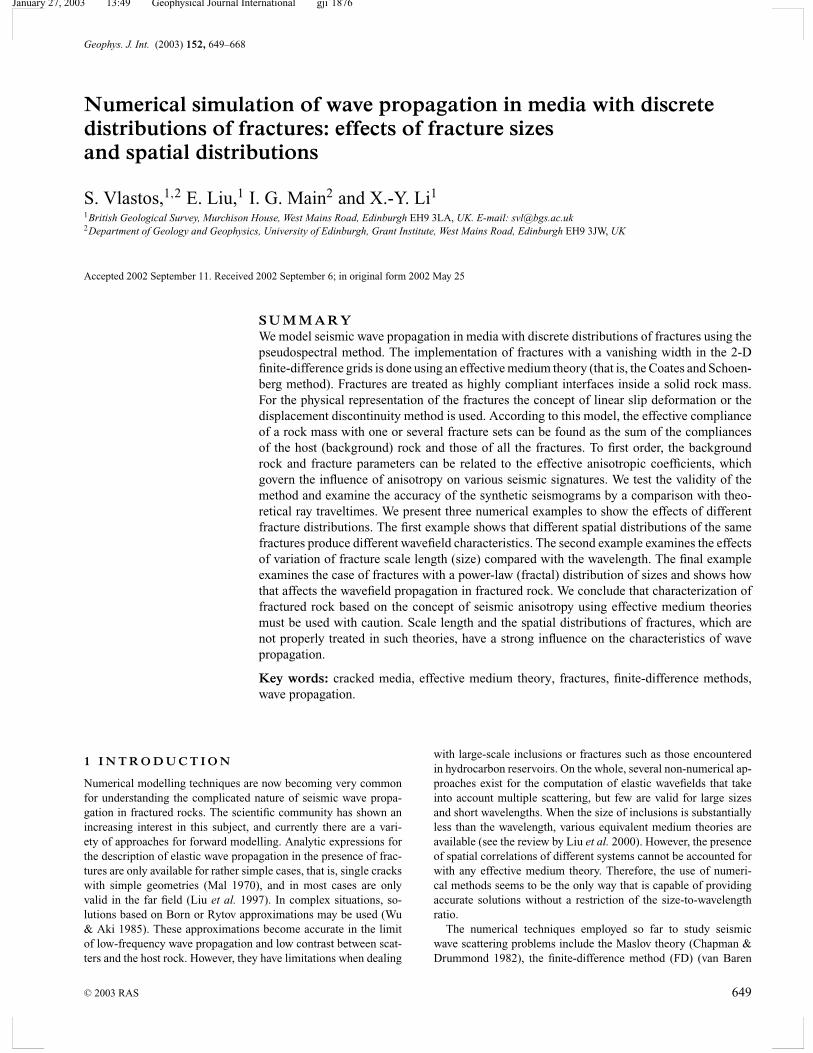
Figure 1. Schematic illustration of fracture discretization in the finite-difference grid. In (a) we show the fractured medium that we want to examine. In(b) we present a very small area of the whole model and (c) shows the same area discretized in the FD grid. Finally, (d) shows again the whole medium where,this time, the fractures are discretized. By comparing (a) and (d) we can see the high accuracy of the discretization.

advantages of the PS method. However, there is a drawback in theuse of the PS method. It intrinsically treats all physical quantitiesas spatially periodic and, as a result, all energy transmitted and re-flected through the boundary will travel back into the grid. Theseartefacts often mask important features of real modelled signals.This deficiency can be mitigated by modifying the wavelet near thegrid boundary in such a way that the wave amplitude is attenuated.

Fractures with a vanishing width in the 2-D finite-differencegrids are implemented using an effective medium theory (fol-lowing Coates & Schoenberg 1995). In the literature, there havebeen several such theories that attempt to predict effective proper-ties of a rockmass containing distributed fractures. In this paper,

C© 2003 RAS, GJI, 152, 649–668


Simulations of wave propagation in fractured rock 651

fractures are treated as highly compliant interfaces inside a solidrock mass. We represent the fractures using the displacement dis-continuity method (DDM) by Schoenberg (1980). We examine thevalidity of the method, and test the accuracy of the synthetics pro-

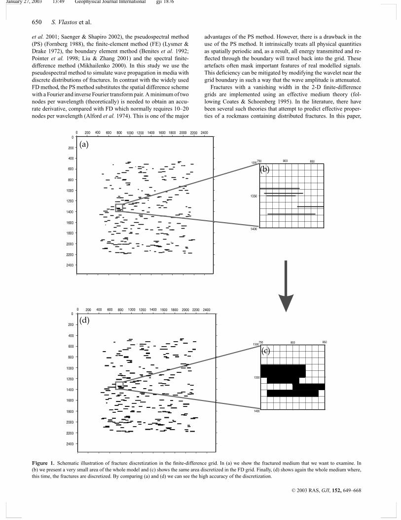
Figure 2. Schematic representation of the model used for the testing ofthe accuracy of the modelling method, and representation of the ray pathsof the different kind of waves generated by the source that interact with thefracture.

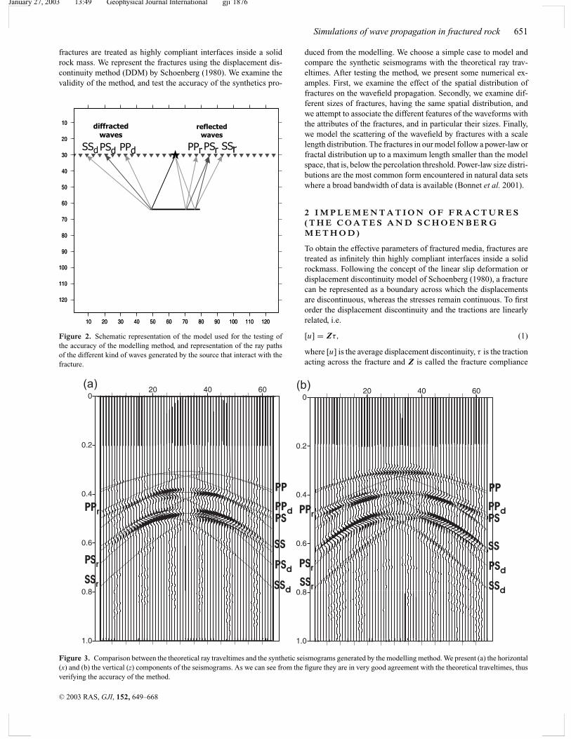
Figure 3. Comparison between the theoretical ray traveltimes and the synthetic seismograms generated by the modelling method. We present (a) the horizontal(x) and (b) the vertical (z) components of the seismograms. As we can see from the figure they are in very good agreement with the theoretical traveltimes, thusverifying the accuracy of the method.

duced from the modelling. We choose a simple case to model andcompare the synthetic seismograms with the theoretical ray trav-eltimes. After testing the method, we present some numerical ex-amples. First, we examine the effect of the spatial distribution offractures on the wavefield propagation. Secondly, we examine dif-ferent sizes of fractures, having the same spatial distribution, andwe attempt to associate the different features of the waveforms withthe attributes of the fractures, and in particular their sizes. Finally,we model the scattering of the wavefield by fractures with a scalelength distribution. The fractures in our model follow a power-law orfractal distribution up to a maximum length smaller than the modelspace, that is, below the percolation threshold. Power-law size distri-butions are the most common form encountered in natural data setswhere a broad bandwidth of data is available (Bonnet et al. 2001).

2 I M P L E M E N T A T I O N O F F R A C T U R E S( T H E C O A T E S A N D S C H O E N B E R GM E T H O D )

To obtain the effective parameters of fractured media, fractures aretreated as infinitely thin highly compliant interfaces inside a solidrockmass. Following the concept of the linear slip deformation ordisplacement discontinuity model of Schoenberg (1980), a fracturecan be represented as a boundary across which the displacementsare discontinuous, whereas the stresses remain continuous. To firstorder the displacement discontinuity and the tractions are linearlyrelated, i.e.

[u] = Zτ, (1)

where [u] is the average displacement discontinuity, τ is the tractionacting across the fracture and Z is called the fracture compliance

C© 2003 RAS, GJI, 152, 649–668



tensor, which is an elastic parameter of the medium. This linearrelationship is consistent with the usual seismic approximation ofinfinitesimal strain. In addition, there has been some experimentalverification of the DDM model by Pyrak-Nolte et al. (1990) andHsu & Schoenberg (1993). Essentially, eq. (1) is a boundary con-dition of the fracture surfaces. In a finite-difference algorithm, therelationship can be implemented by requiring a displacement jumpacross gridpoints on either side of the interface, proportional to thelocal (continuous) stress traction. The implementation of the dis-placement jump is relatively simple, even with Z being a functionof position on the fault plane, providing the interface lies along agiven plane of the finite-difference grid. In nature, fractures havefinite length. To implement a finite fracture we take Z = 0 at loca-tions on the plane exterior to the fracture. The question that remainsis how to implement the constraint that Z → 0 on the tips of thefracture. We taper off the value of Z following the formulation of the

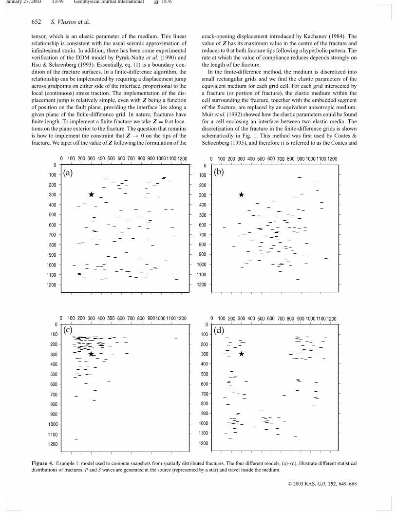
Figure 4. Example 1: model used to compute snapshots from spatially distributed fractures. The four different models, (a)–(d), illustrate different statisticaldistributions of fractures. P and S waves are generated at the source (represented by a star) and travel inside the medium.

crack-opening displacement introduced by Kachanov (1984). Thevalue of Z has its maximum value in the centre of the fracture andreduces to 0 at both fracture tips following a hyperbolic pattern. Therate at which the value of compliance reduces depends strongly onthe length of the fracture.

In the finite-difference method, the medium is discretized intosmall rectangular grids and we find the elastic parameters of theequivalent medium for each grid cell. For each grid intersected bya fracture (or portion of fracture), the elastic medium within thecell surrounding the fracture, together with the embedded segmentof the fracture, are replaced by an equivalent anisotropic medium.Muir et al. (1992) showed how the elastic parameters could be foundfor a cell enclosing an interface between two elastic media. Thediscretization of the fracture in the finite-difference grids is shownschematically in Fig. 1. This method was first used by Coates &Schoenberg (1995), and therefore it is referred to as the Coates and

C© 2003 RAS, GJI, 152, 649–668



Schoenberg method in this paper. In Fig. 1(a) we show the wholefractured medium. Then we take a very small area of the mediumin Fig. 1(b), to show how the fractures are represented in the finite-difference grid. Fig. 1(c) shows the discretization of the fractures inthe grid, where the shaded areas are the finite-difference grid cellsintersected by one or more fractures, whilst the plain areas are thecells that include only the background rock. Finally, in Fig. 1(d)we show the whole medium again, but this time each cell is eithershaded or plain, depending on whether fractures are present. Bycomparing Fig. 1(d) with Fig. 1(a), where we show the mediumwith the actual fractures, we can see that the discretization of thefractures is very accurate. In the numerical examples presented inthis paper we use in some cases a grid size of 128 × 128 and inother cases 256 × 256. The grid cell size is very important for thediscretization of the fractures. To achieve high accuracy, we choosegrid sizes smaller than or equal to the size of the smallest fractures.

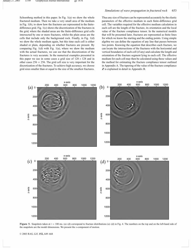
Figure 5. Snapshots taken at t = 100 ms. (a)–(d) correspond to fracture distributions (a)–(d) in Fig. 4. The numbers on the top and on the left-hand side ofthe snapshots are the model dimensions. We present the x-component of motion.

Thus any size of fracture can be represented accurately by the elasticparameters of the effective medium in each finite-difference gridcell. The variables required for the effective medium calculation ineach cell are the length of the fracture, its orientation and the localvalue of the fracture compliance tensor. In the numerical modelsthat will be presented later, fractures are represented as finite linesfor which we know the starting and the ending points. Using simplealgebra we can define the equation of any line that passes betweentwo points. Knowing the equation that describes each fracture, wecan locate the intersections of the fractures with the horizontal andvertical boundaries of each cell (if any) and calculate the length andorientation of the fracture segment lying in each cell. The effectivemedium for each cell may then be calculated using these values andthe method for estimating the fracture compliance tensor outlinedin Appendix A. The tapering of the value of the fracture complianceZ is explained in detail in Appendix B.

C© 2003 RAS, GJI, 152, 649–668



3 VA L I D A T I O N

The first step is to compare results generated by our modellingmethod with those obtained by another method. This has been doneby Coates & Schoenberg (1995), Nihei & Myer (2000) and Niheiet al. (2000), who compared the synthetic seismograms from theCoates and Schoenberg method described with the exact solutionsusing boundary element methods. We assess the accuracy by com-paring the synthetic seismograms generated by the modelling withthe ray theoretical traveltimes.

The model geometry used for accuracy testing is shown in Fig. 2.The source, receivers and fracture are situated in an ideal elastic(V P = 3300 m s−1, V S = 1800 m s−1, ρ = 2200 kg m−3) full space.The receiver array at which vertical and horizontal particle displace-ments are recorded is horizontal and 340 m above the fracture. Thefracture is 300 m long. The source is located at the centre of thereceiver array. The source type is a vertical force. The source signalis a Ricker wavelet (Ricker 1977) with a peak frequency of 25 Hz

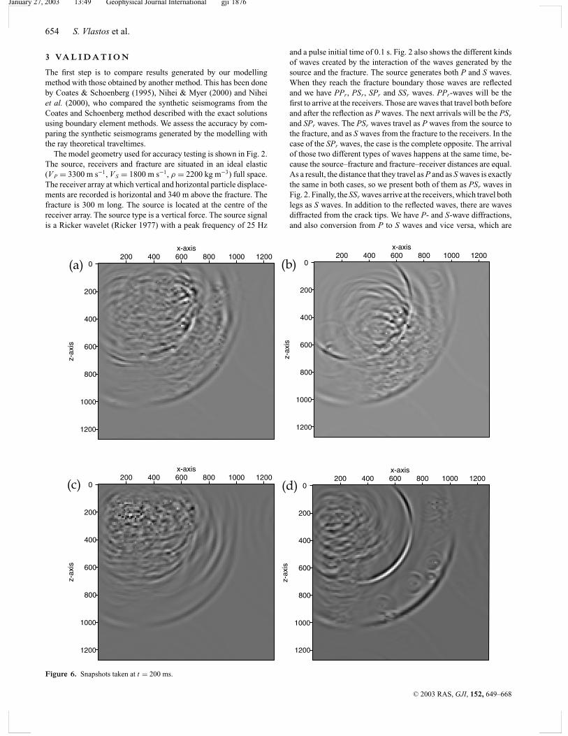
Figure 6. Snapshots taken at t = 200 ms.

and a pulse initial time of 0.1 s. Fig. 2 also shows the different kindsof waves created by the interaction of the waves generated by thesource and the fracture. The source generates both P and S waves.When they reach the fracture boundary those waves are reflectedand we have PPr, PSr, SPr and SSr waves. PPr-waves will be thefirst to arrive at the receivers. Those are waves that travel both beforeand after the reflection as P waves. The next arrivals will be the PSr

and SPr waves. The PSr waves travel as P waves from the source tothe fracture, and as S waves from the fracture to the receivers. In thecase of the SPr waves, the case is the complete opposite. The arrivalof those two different types of waves happens at the same time, be-cause the source–fracture and fracture–receiver distances are equal.As a result, the distance that they travel as P and as S waves is exactlythe same in both cases, so we present both of them as PSr waves inFig. 2. Finally, the SSr waves arrive at the receivers, which travel bothlegs as S waves. In addition to the reflected waves, there are wavesdiffracted from the crack tips. We have P- and S-wave diffractions,and also conversion from P to S waves and vice versa, which are

C© 2003 RAS, GJI, 152, 649–668



diffracted from the tips of the fracture. These waves are presentedin Fig. 2 as PPd , PSd , SPd and SSd waves.

We calculate the theoretical ray traveltimes and overlap them onthe synthetic seismograms. Figs 3(a) and (b) show the horizontal(x) and the vertical (z) components, respectively, of the syntheticseismograms together with the theoretical ray traveltimes. As wecan see from both figures, we have very good agreement between thetheoretical ray traveltimes and the synthetic seismograms. All typesof waves are accurately represented in the synthetic seismograms.Owing to the type of source that we implement, we have strongarrivals at short offsets on the horizontal component and strongarrivals at long offsets on the vertical component. In addition to that,the diffracted waves from the tips of the fracture and the PPr andPPd waves are not visible in the horizontal component, but they arevery clearly demonstrated in the vertical component and follow thetheoretical traveltimes. This is expected because the source causesvertical displacements on the medium, so very close to the sourceand very far away from it, the horizontal displacement is negligible.

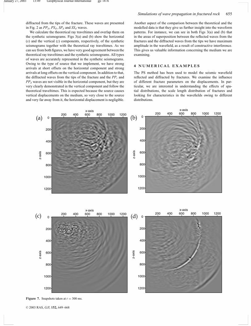
Figure 7. Snapshots taken at t = 300 ms.

Another aspect of the comparison between the theoretical and themodelled data is that they give us further insight into the waveformpatterns. For instance, we can see in both Figs 3(a) and (b) thatin the areas of superposition between the reflected waves from thefractures and the diffracted waves from the tips we have maximumamplitude in the wavefield, as a result of constructive interference.This gives us valuable information concerning the medium we areexamining.

4 N U M E R I C A L E X A M P L E S

The PS method has been used to model the seismic wavefieldreflected and diffracted by fractures. We examine the influenceof different fracture parameters on the displacements. In par-ticular, we are interested in understanding the effects of spa-tial distributions, the scale length distribution of fractures andlooking for characteristics in the wavefields owing to differentdistributions.

C© 2003 RAS, GJI, 152, 649–668



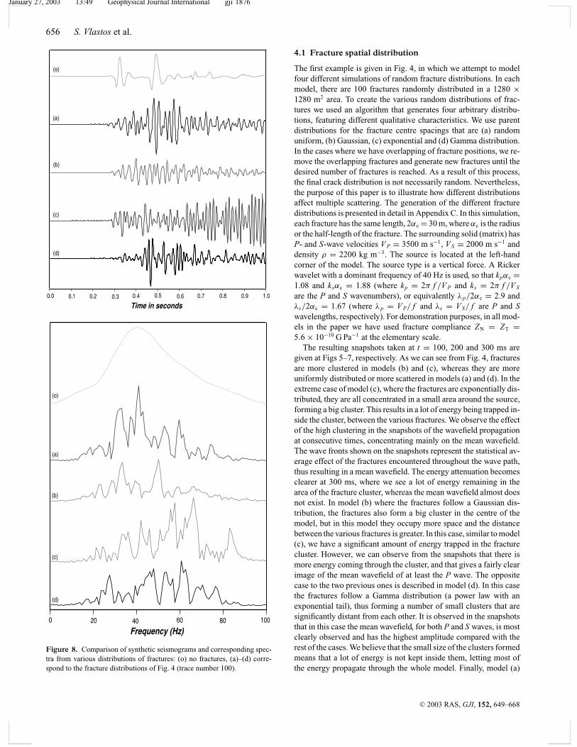
Figure 8. Comparison of synthetic seismograms and corresponding spec-tra from various distributions of fractures: (o) no fractures, (a)–(d) corre-spond to the fracture distributions of Fig. 4 (trace number 100).

4.1 Fracture spatial distribution

The first example is given in Fig. 4, in which we attempt to modelfour different simulations of random fracture distributions. In eachmodel, there are 100 fractures randomly distributed in a 1280 ×1280 m2 area. To create the various random distributions of frac-tures we used an algorithm that generates four arbitrary distribu-tions, featuring different qualitative characteristics. We use parentdistributions for the fracture centre spacings that are (a) randomuniform, (b) Gaussian, (c) exponential and (d) Gamma distribution.In the cases where we have overlapping of fracture positions, we re-move the overlapping fractures and generate new fractures until thedesired number of fractures is reached. As a result of this process,the final crack distribution is not necessarily random. Nevertheless,the purpose of this paper is to illustrate how different distributionsaffect multiple scattering. The generation of the different fracturedistributions is presented in detail in Appendix C. In this simulation,each fracture has the same length, 2αc = 30 m, where αc is the radiusor the half-length of the fracture. The surrounding solid (matrix) hasP- and S-wave velocities V P = 3500 m s−1, V S = 2000 m s−1 anddensity ρ = 2200 kg m−3. The source is located at the left-handcorner of the model. The source type is a vertical force. A Rickerwavelet with a dominant frequency of 40 Hz is used, so that kpαc =1.08 and ksαc = 1.88 (where kp = 2π f /V P and ks = 2π f /V S

are the P and S wavenumbers), or equivalently λp/2αc = 2.9 andλs/2αc = 1.67 (where λp = V P/ f and λs = V S/ f are P and Swavelengths, respectively). For demonstration purposes, in all mod-els in the paper we have used fracture compliance ZN = ZT =5.6 × 10−10 G Pa−1 at the elementary scale.

The resulting snapshots taken at t = 100, 200 and 300 ms aregiven at Figs 5–7, respectively. As we can see from Fig. 4, fracturesare more clustered in models (b) and (c), whereas they are moreuniformly distributed or more scattered in models (a) and (d). In theextreme case of model (c), where the fractures are exponentially dis-tributed, they are all concentrated in a small area around the source,forming a big cluster. This results in a lot of energy being trapped in-side the cluster, between the various fractures. We observe the effectof the high clustering in the snapshots of the wavefield propagationat consecutive times, concentrating mainly on the mean wavefield.The wave fronts shown on the snapshots represent the statistical av-erage effect of the fractures encountered throughout the wave path,thus resulting in a mean wavefield. The energy attenuation becomesclearer at 300 ms, where we see a lot of energy remaining in thearea of the fracture cluster, whereas the mean wavefield almost doesnot exist. In model (b) where the fractures follow a Gaussian dis-tribution, the fractures also form a big cluster in the centre of themodel, but in this model they occupy more space and the distancebetween the various fractures is greater. In this case, similar to model(c), we have a significant amount of energy trapped in the fracturecluster. However, we can observe from the snapshots that there ismore energy coming through the cluster, and that gives a fairly clearimage of the mean wavefield of at least the P wave. The oppositecase to the two previous ones is described in model (d). In this casethe fractures follow a Gamma distribution (a power law with anexponential tail), thus forming a number of small clusters that aresignificantly distant from each other. It is observed in the snapshotsthat in this case the mean wavefield, for both P and S waves, is mostclearly observed and has the highest amplitude compared with therest of the cases. We believe that the small size of the clusters formedmeans that a lot of energy is not kept inside them, letting most ofthe energy propagate through the whole model. Finally, model (a)

C© 2003 RAS, GJI, 152, 649–668



where fractures are randomly uniformly distributed, describes a casewhere we do not have any clustering. The fractures are distributedthroughout the whole medium. Although the snapshots show sometrapped energy between the fractures, the mean wavefield propaga-tion is quite clearly observed. To sum up the results, we can see thatthe wavefield propagates with the least energy attenuation when wehave the least fracture clustering as shown in model (d), while atten-uation increases with increasing clustering as shown in models (a)–(c), respectively.In the following, we take the models of Fig. 4 and calculate thesynthetic seismograms. The receivers are positioned along thez-direction and shifted by 1050 m in the x-direction. The caseswe compare are (o) no fractures, (a) random uniform distribu-tion, (b) Gaussian distribution, (c) exponential distribution and (d)Gamma distribution. Fig. 8 shows comparisons of waveforms of thex-component of motion from trace number 100, that corresponds tothe depth of 1000 m, of each of the models and their correspond-ing Fourier spectra. In the figure we observe a noticeable shift of

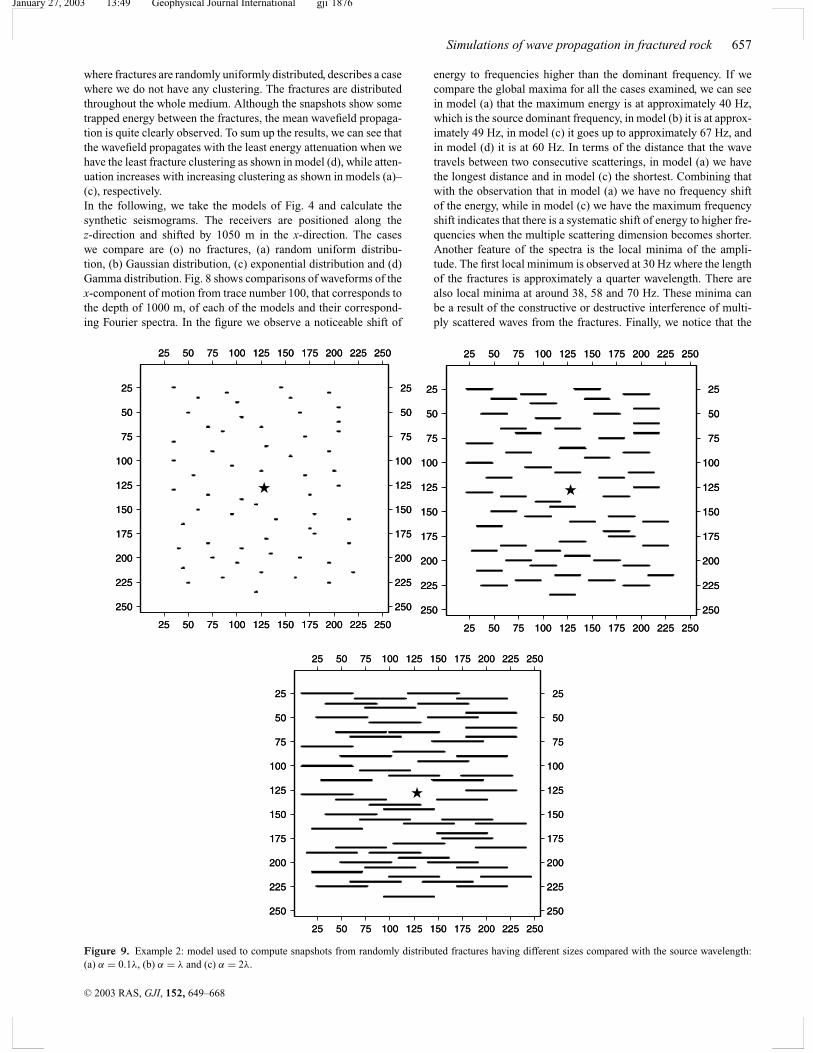
Figure 9. Example 2: model used to compute snapshots from randomly distributed fractures having different sizes compared with the source wavelength:(a) α = 0.1λ, (b) α = λ and (c) α = 2λ.

energy to frequencies higher than the dominant frequency. If wecompare the global maxima for all the cases examined, we can seein model (a) that the maximum energy is at approximately 40 Hz,which is the source dominant frequency, in model (b) it is at approx-imately 49 Hz, in model (c) it goes up to approximately 67 Hz, andin model (d) it is at 60 Hz. In terms of the distance that the wavetravels between two consecutive scatterings, in model (a) we havethe longest distance and in model (c) the shortest. Combining thatwith the observation that in model (a) we have no frequency shiftof the energy, while in model (c) we have the maximum frequencyshift indicates that there is a systematic shift of energy to higher fre-quencies when the multiple scattering dimension becomes shorter.Another feature of the spectra is the local minima of the ampli-tude. The first local minimum is observed at 30 Hz where the lengthof the fractures is approximately a quarter wavelength. There arealso local minima at around 38, 58 and 70 Hz. These minima canbe a result of the constructive or destructive interference of multi-ply scattered waves from the fractures. Finally, we notice that the

C© 2003 RAS, GJI, 152, 649–668



amplitude of the wavefield from distribution (b) is much smallerand has a relatively low-frequency content compared with the otherdistributions. This is possibly because in this case the local fracturedensity along the wave path towards the receivers is higher comparedwith the other cases. This example demonstrates clearly that differ-ent distributions of fractures have a significant influence on multiplescattering.

4.2 Effects of fracture scale length

The second example is used to examine wave scattering in a frac-tured medium where fractures have different sizes compared withthe source wavelength. To ensure consistency of the results fromdifferent models we use the same background medium in all cases,which guarantees that any variation in the features of the wavefieldis a result of the variation in the size of the fractures. The matrixparameters are V P = 3300 m s−1 and V S = 1800 m s−1 for the

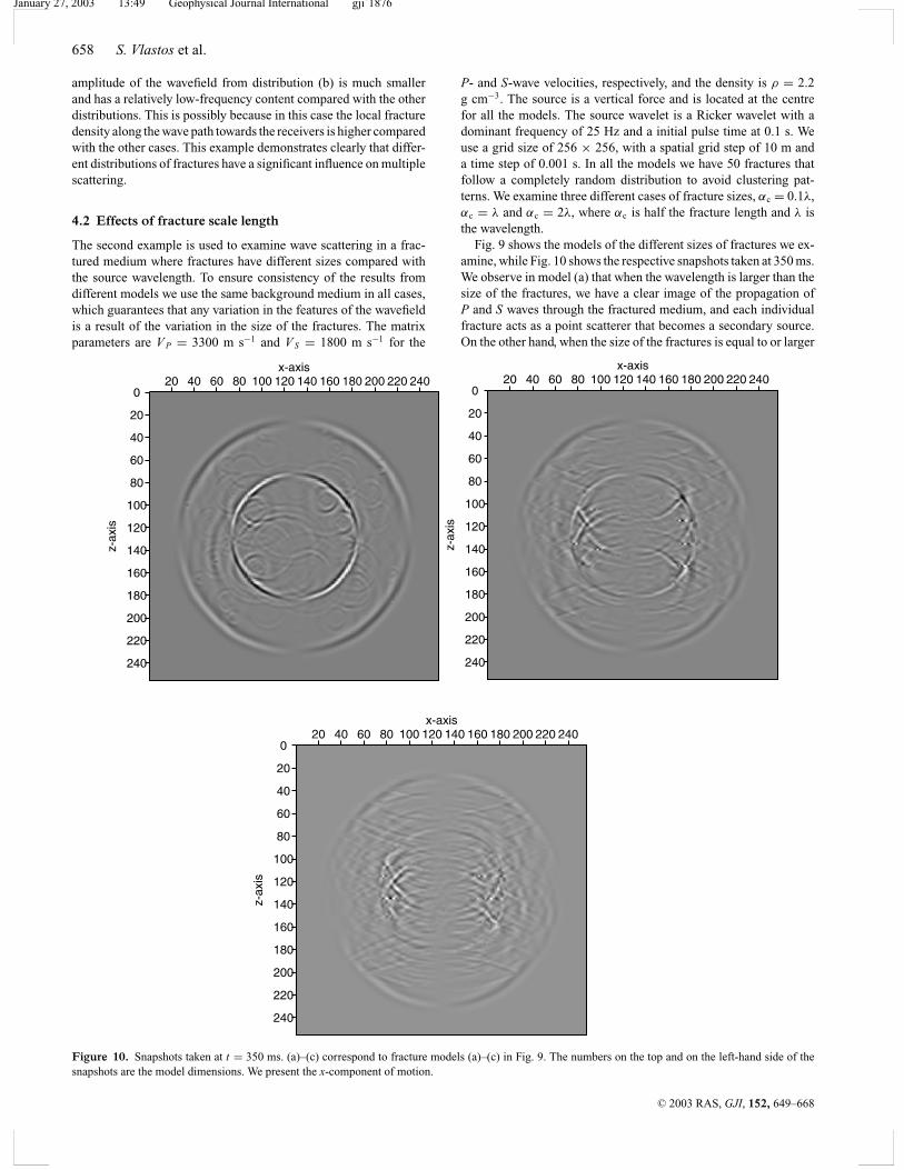
Figure 10. Snapshots taken at t = 350 ms. (a)–(c) correspond to fracture models (a)–(c) in Fig. 9. The numbers on the top and on the left-hand side of thesnapshots are the model dimensions. We present the x-component of motion.

P- and S-wave velocities, respectively, and the density is ρ = 2.2g cm−3. The source is a vertical force and is located at the centrefor all the models. The source wavelet is a Ricker wavelet with adominant frequency of 25 Hz and a initial pulse time at 0.1 s. Weuse a grid size of 256 × 256, with a spatial grid step of 10 m anda time step of 0.001 s. In all the models we have 50 fractures thatfollow a completely random distribution to avoid clustering pat-terns. We examine three different cases of fracture sizes, αc = 0.1λ,αc = λ and αc = 2λ, where αc is half the fracture length and λ isthe wavelength.

Fig. 9 shows the models of the different sizes of fractures we ex-amine, while Fig. 10 shows the respective snapshots taken at 350 ms.We observe in model (a) that when the wavelength is larger than thesize of the fractures, we have a clear image of the propagation ofP and S waves through the fractured medium, and each individualfracture acts as a point scatterer that becomes a secondary source.On the other hand, when the size of the fractures is equal to or larger

C© 2003 RAS, GJI, 152, 649–668



than the wavelength, they act almost as individual boundaries andthe amplitudes of the reflected waves depend on the interference be-tween the various reflections. In addition, following the results of theprevious section on the effects of the fracture distribution togetherwith the effects of the scale length, strong and coherent energy willbe present in areas of high fracture clustering where fractures formlarge clusters and have a large size, thus acting as a single reflector.

4.3 Power-law (fractal) distribution of fracture sizes

The final example is used to model wave scattering from discretefractures with a scale length distribution. The model we use isgiven in Fig. 11(a), where the variation of crack sizes follows avon Karman correlation function, which gives a power-law distri-

Figure 11. (a) Example 3: model used to compute synthetic seismograms from fracture distribution with power-law distribution of fracture sizes. (b) Illustrationof the sizes of fractures in model (a), that follow a power-law distribution. (c) Power spectra of fracture size distributions shown in (a). (d) Cumulative numberof the fractures of model (a) plotted against the fracture size.

bution (Wu 1982). We can also use other correlation functions, suchas Gaussian or exponential functions. The model shown in Fig. 11(a)is generated with a correlation length of 40 m. In this model we have400 fractures randomly distributed in a 2560 × 2560 m2 area. Thesource is a vertical force and is located in the centre of the model, andis represented by a star in Fig. 11(a). The longest fracture is 100 mand the shortest is 10 m. The mean length of the fractures 〈a〉 is27.5 m, and the fracture density of the medium ε = N f〈a〉2/S is0.046, where N f is the number of fractures and S is the surface ofthe medium. The peak frequency is 40 Hz, which gives α rangingfrom 0.36 to 3.6 for P waves and from 0.63 to 6.3 for S waves,where k is the wavenumber, the P-wave velocity is 3500 m s−1 andthe S-wave velocity is 2000 m s−1. Figs 11(b)–(d), illustrate the at-tributes of the size distribution of the fractures. Fig. 11(b) showsthe different sizes of fractures in the model of Fig. 11(a). Fig. 11(c)

C© 2003 RAS, GJI, 152, 649–668



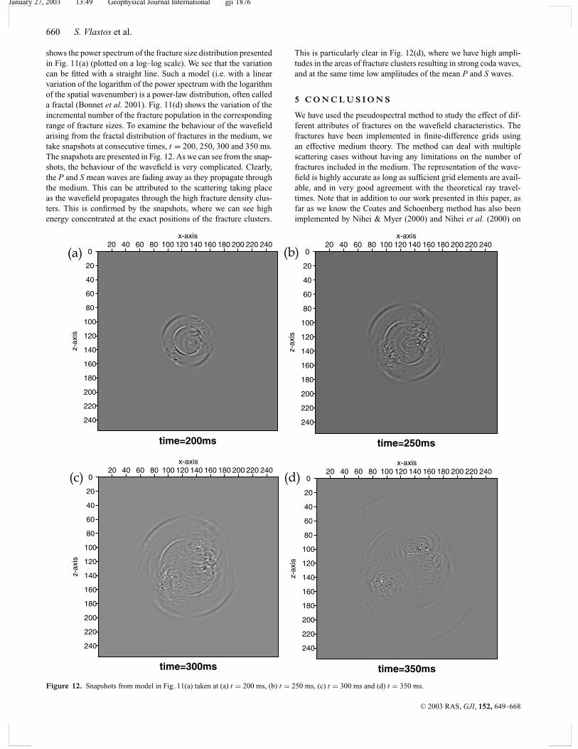
shows the power spectrum of the fracture size distribution presentedin Fig. 11(a) (plotted on a log–log scale). We see that the variationcan be fitted with a straight line. Such a model (i.e. with a linearvariation of the logarithm of the power spectrum with the logarithmof the spatial wavenumber) is a power-law distribution, often calleda fractal (Bonnet et al. 2001). Fig. 11(d) shows the variation of theincremental number of the fracture population in the correspondingrange of fracture sizes. To examine the behaviour of the wavefieldarising from the fractal distribution of fractures in the medium, wetake snapshots at consecutive times, t = 200, 250, 300 and 350 ms.The snapshots are presented in Fig. 12. As we can see from the snap-shots, the behaviour of the wavefield is very complicated. Clearly,the P and S mean waves are fading away as they propagate throughthe medium. This can be attributed to the scattering taking placeas the wavefield propagates through the high fracture density clus-ters. This is confirmed by the snapshots, where we can see highenergy concentrated at the exact positions of the fracture clusters.

Figure 12. Snapshots from model in Fig. 11(a) taken at (a) t = 200 ms, (b) t = 250 ms, (c) t = 300 ms and (d) t = 350 ms.

This is particularly clear in Fig. 12(d), where we have high ampli-tudes in the areas of fracture clusters resulting in strong coda waves,and at the same time low amplitudes of the mean P and S waves.

5 C O N C L U S I O N S

We have used the pseudospectral method to study the effect of dif-ferent attributes of fractures on the wavefield characteristics. Thefractures have been implemented in finite-difference grids usingan effective medium theory. The method can deal with multiplescattering cases without having any limitations on the number offractures included in the medium. The representation of the wave-field is highly accurate as long as sufficient grid elements are avail-able, and in very good agreement with the theoretical ray travel-times. Note that in addition to our work presented in this paper, asfar as we know the Coates and Schoenberg method has also beenimplemented by Nihei & Myer (2000) and Nihei et al. (2000) on

C© 2003 RAS, GJI, 152, 649–668



staggered grid FDs, and by Chunlin Wu on variable grid FDs (Wuet al. 2002).

From the numerical examples we come to some interesting con-clusions. First, we can see the importance of the spatial distributionof fractures in a medium. Our results show that in areas with fractureclustering, there is strong and coherent energy. Also, high cluster-ing does result in high local fracture densities, which can causethe energy to be trapped in a certain area (localization processing),increasing the complexity of the wavefield and making individualphases and their identification very complicated. Also, we observethat different spatial distributions give different frequency contenton the recorded wavefield. This as we might expect means thatfrequency-dependent seismic scattering depends on the spatial dis-tribution of fractures (Leary & Abercrombie 1994). In addition, alsoof great importance is the fracture size relative to the wavelength,independent of the spatial distribution. It is demonstrated that whenfractures are smaller than the wavelength, they act as single scat-terers and generate secondary wavefields, whereas when the sizeapproaches the wavelength they act as individual interfaces and thewavefield is more complicated. To complete our study, we examinedthe case of fracture sizes that follow a power-law or fractal distri-bution. The wavefield generated shows very strong coda waves andis very complicated. The observation confirms the importance ofspatial and scale length distributions in modelling fractured rock.

Numerical modelling techniques, such as those presented here,can be a useful tool in the understanding of the important role offractures and their effects on wave propagation. The knowledgegained by such studies may ultimately lead to the extraction ofvaluable information concerning the fracture distributions in nat-ural rocks, directly from seismic data. In addition, our method maypotentially provide a test of fracture imaging using seismic meth-ods (as demonstrated by Nihei et al. 2000), and characterization offractured reservoirs based on the concept of seismic scattering.

6 C O L O U R O N L I N E

Colour versions of Figs 2, 3, 8 and B1 are available online at Black-well Synergy, www.blackwell-synergy.com.

A C K N O W L E D G M E N T S

We thank Kurt Nihei, Seiji Nakagawa and Michael Schoenberg(Lawrence Berkley National Laboratory), Chunling Wu (StanfordUniversity), John Queen (Conoco Inc.), Zhang Zhongjie, XinwuZeng (Chinese Academy of Sciences), and our colleagues PatienceCowie, Mark Chapman and Simon Tod for useful discussion con-cerning natural fracture distributions and fracture modelling. Wethank GJI reviewer Thomas Daley and an anonymous reviewer andEditor Michael Korn for their constructive comments. We also thankJoe Dellinger of BP for reminding us of the paper by Muir et al.(1992). This research is supported by the sponsors of the EdinburghAnisotropy Project. This work is published with the permission ofthe Executive Director of the British Geological Survey (NERC) andthe EAP sponsors: BP, Chevron, Conoco, DTI, ENI-Agip, Exxon-Mobil, Norsk Hydro, PGS, Phillips, Schlumberger, Texaco, TradePartners UK and Veritas DGC.

R E F E R E N C E S

Alford, R.M., Kelly, K.R. & Boore, D.M., 1974. Accuracy of finite-difference modelling of the acoustic wave equation, Geophysics, 39, 834–842.

Benites, R., Aki, K. & Yomogida, K., 1992. Multiple scattering of SH wavesin 2-D media with many cavities, Pure appl. Geophys., 138, 353–390.

Bonnet, E., Bour, O., Odling, N.E., Davy, P., Main, I., Cowie, P. & Berkowitz,B., 2001. Scaling of fracture systems in geological media, Rev. Geophys.,39, 347–383.

Chapman, C.H. & Drummond, R., 1982. Body-wave seismograms in inho-mogeneous media using Maslov asymptotic theory, Bull. seism. Soc. Am.,72, 277–317.

Coates, R.T. & Schoenberg, M., 1995. Finite-difference modeling of faultsand fractures, Geophysics, 60, 1514–1526.

Fornberg, B., 1988. The pseudospectral method: accurate representation ofinterfaces in elastic wave calculations, Geophysics, 53, 625–637.

Hentschel, H.G.E. & Proccacia, I., 1983. The infinite number of generaliseddimensions of fractals and strange attractors, Physica D, 8, 435–444.

Hill, R., 1963. Elastic properties of reinforced solids: some theoretical prin-ciples, J. mech. Phys. Solids, 11, 357–372.

Hsu, C.-J. & Schoenberg, M., 1993. Elastic waves through a simulated frac-tured medium, Geophysics, 58, 964–977.

Hudson, J.A. & Knopoff, L., 1989. Predicting the overall properties of com-posite materials with small-scale inclusions or cracks, Pure appl. Geo-phys., 131, 551–576.

Kachanov, M., 1984. Elastic solids with many cracks and related problems,Adv. Appl. Mech., 30.

Leary, P.C. & Abercrombie, R., 1994. Frequency dependent crustal scatter-ing & absorption at 5–160 Hz from coda decay observed at 2–5 km depth,Geophys. Res. Lett., 21, 971–974.

Liu, E. & Zhang, Z., 2001. Numerical study of elastic wave scattering bycracks or inclusions using the boundary integral equation method, J. comp.Acoust., 9, 1039–1054.

Liu, E., Crampin, S. & Hudson, J.A., 1997. Diffraction of seismic waveswith application to hydraulic fracturing, Geophysics, 62, 253–265.

Liu, E., Hudson, J.A. & Pointer, T., 2000. Equivalent medium representationof fractured rock, J. geophys. Res., 105, 2981–3000.

Lysmer, J. & Drake, L.A., 1972. A finite element method for seismology,Methods Computat. Phys., 11, Academic Press, New York.

Mal, A.K., 1970. Interaction of elastic waves with a Griffith crack, Int. J.eng. Sci., 8, 763–776.

Mikhailenko, B.G., 2000. Seismic modeling by the spectral-finite differencemethod, Phys. Earth planet. Inter., 119, 133–147.

Muir, F., Dellinger, D., Etgen, J. & Nichols, D., 1992. Modeling elasticwavefields across irregular boundaries, Geophysics, 57, 1189–1193.

Nihei, K.T. & Myer, L.R., 2000. Natural fracture characterisation usingpassive seismic waves, Gas Tips, Gas Technology Institute, US Dept. ofEnergy and Hart Publications Inc.

Nihei, K.T., Nakagawa, S. & Myer, L.R., 2000. VSP fracture imaging withelastic reverse-time migration, 70th Ann. Int. Mtg.: Soc. of Expl. Geophys.,1784–1751.

Pointer, T., Liu, E. & Hudson, J.A., 1998. Numerical modelling of seismicwaves scattered by hydrofractures: application of the indirect boundaryelement method, Geophys. J. Int. 135, 289–303.

Press, W.H., Teukolsky, S.A., Vetterling, W.T. & Flannery, B.P., 1997. Nu-merical Recipes in Fortran 77: the Art of Scientific Computing (Vol. 1 ofFortran Numerical Recipies), pp. 266–283, Cambridge University Press,Cambridge.

Pyrak-Nolte, L.J., Myer, L.R. & Cook, N.G.W., 1990. Transmission of seis-mic waves accross single natural fractures, J. geophys. Res., 95, 8617–8638.

Ricker, N.H., 1977. Transient Waves in Visco-elastic Media, Elsevier,Amsterdam.

Saenger, E.H. & Shapiro, S.A., 2002. Effective velocities in fractured me-dia: a numerical study using the rotated staggered finite-difference grid,Geophys. Prosp., 50, 183–194.

Sayers, C.M. & Kachanov, M., 1995. Microcrack-induced elastic waveanisotropy of brittle rocks, J. geophys. Res., 100, 4149–4156.

Schoenberg, M., 1980. Elastic wave behaviour across linear slip interfaces,J. acoust. Soc. Am., 68, 1516–1521.

Schoenberg, M. & Sayers, C.M., 1995. Seismic anisotropy of fractured rock,Geophysics, 60, 204–211.

C© 2003 RAS, GJI, 152, 649–668



van Baren, G.B., Mulder, W.A. & Herman, G.C., 2001. Finite-differencemodeling of scalar-wave propagation in cracked media, Geophysics, 66,267–276.

Wu, C., Harris, J.M. & Nihei, K.T., 2002. 2-D finite-difference seismic mod-elling of an open fluid-filled fracture comparison of thin-layer and linear-slip models, 72nd SEG Ann. Int. Mtg. Exp. Abs.: Soc. of Expl. Geophys.,1959–1962.

Wu, R.S., 1982. Attenuation of short period seismic waves due to scattering,Geophys. Res. Lett., 9, 9–12.

Wu, R.S. & Aki, K., 1985. Scattering characteristics of elastic waves by anelastic heterogeneity, Geophysics, 50, 582–589.

A P P E N D I X A : E F F E C T I V EC O M P L I A N C E O F A F R A C T U R E DM E D I U M

Effective medium calculus is used to calculate the elastic parame-ters that are associated with a given cell through which a fracturepasses. In the simple case of an unfractured cell, where the cell isoccupied only by the background rock, the calculation of the com-pliance tensor is straightforward. Assuming that we know the elasticparameters of the host rock, we calculate the compliance tensor s0

ijkl

as follows:

µ = ρV 2s , (A1)

λ = ρ(V 2

P − 2V 2S

), (A2)

(s0

i jkl

)−1 = ci jkl =

λ + 2µ λ λ 0 0 0

λ λ + 2µ λ 0 0 0

λ λ λ + 2µ 0 0 0

0 0 0 µ 0 0

0 0 0 0 µ 0

0 0 0 0 0 µ

,

(A3)

where V P and V S are the P- and S-wave velocities in the medium,respectively, cijkl is the 6 × 6 matrix form of the stiffness tensor forthe unfractured medium, and λ and µ are the Lame constants.

In the presence of fractures the average strain ε in an elastichomogeneous solid with volume V containing N f fractures withsurfaces Sr (r = 1, 2, . . . , N f) can be written as

εi j = (s0

i jkl + s fi jkl

)σkl , (A4)

where σ is the average stress tensor, s0ijkl is the matrix compliance

tensor in the absence of the fractures and s fijkl is the extra compliance

tensor resulting from the fractures. The additional strain is given by(Hill 1963; Hudson & Knopoff 1989),

s fi jklσkl = 1

2V

Nf∑r=1

∫Sr

([ui ]n j + [u j ]ni ) d S, (A5)

where ui is the ith component of the displacement discontinuity onSr and ni is the ith component of the fracture normal. If all fracturesare aligned with fixed normal n, we may replace each fracture in Vby an average fracture having a surface area S and a smoothed linearslip boundary condition given by

[ui ] = Ziptp, (A6)

where tp is the traction on the fracture, [ui ] is the average displace-ment discontinuity on the fracture and the quantities{Zip}depend onthe interior conditions and infill of the fracture (Sayers & Kachanov1995; Schoenberg & Sayers 1995). The traction tp is linearly relatedto the imposed mean stressσ or, more precisely, to the traction σ pqnq

that would exist on the crack face if the displacements were con-strained to be zero.

Liu et al. (2000) used a model of a simple fracture in an unboundedmedium and proposed that the traction can be written as

tp = σpq nq , (A7)

eq. (A6) becomes

[ui ] = Zipσpq nq . (A8)

Inserting eq. (A8) into eq. (A5) and after some tensor algebra, weobtain

s fi jklσkl = Nf S

4V(Ziknln j + Z jknlni + Zilnkn j + Z jlnkni )σkl ,

(A9)

where S is the mean area of fracture; so the fracture induced excesscompliance s f

ijkl is

s fi jkl = Df

4(Ziknln j + Z jknlni + Zilnkn j + Z jlnkni ), (A10)

where Df is

Df = Nf S

V. (A11)

If the fracture set is statistically invariant under rotations about n,only two terms in Z are required (Schoenberg & Sayers 1995); anormal fracture compliance ZN and a tangential compliance ZT.Thus

Zi j = ZNni n j + ZT(δi j − ni n j ) = ZTδi j + (ZN − ZT)ni n j ,

(A12)

where δi j is the Kronecker delta. By inserting (A12) into (A10), wehave

s fi jkl = Df

4[ZT(δiknln j + δ jknlni + δil nkn j + δ jl nkni )

+ 4(ZN − ZT)ni n j nknl ]. (A13)

Following Coates & Schoenberg (1995), in the case of 2-D mediain a grid cell intersected by a fracture, eq. (A11) becomes

Df = Nf�l

�A, (A14)

where �l is the length of the segment of the fracture lying withinthe cell and �A is the area of the 2-D cell. If L is defined for eachcell intersected by a fracture so that

1

L≡ �l

�A, (A15)

then eq. (A13) finally becomes

s fi jkl = Nf

4L[ZT(δiknln j + δ jknlni + δil nkn j + δ jl nkni )

+ 4(ZN − ZT)ni n j nknl ], (A16)

which is the equation we use for the calculation of the excess com-pliance tensor. So the induced excess compliance tensor of a celldepends on the normal ZN and the tangential ZT fracture compli-ance, the number N f of the fractures inside the cell, the length �lof each fracture (or segment of fracture) and the orientation of eachfracture estimated by the normals n. The total compliance tensorfor the fractured cells is the effective compliance tensor seff

ijkl, whichcharacterizes the cell and is

seffi j = s0

i jkl + s fi jkl . (A17)

C© 2003 RAS, GJI, 152, 649–668



If we want to determine the stiffness cijkl, we transform sijkl tothe conventional (two-subscript) condensed 6 × 6 matrix notation,11 → 1, 22 → 2, 33 → 3, 23 → 4, 13 → 5, 12 → 6, with factorsof 2 and 4 introduced as follows: sijkl → spq when both of P, q are 1,2, or 3; 2sijkl → spq when one of p, q is 4, 5 or 6; and 4sijkl → spq whenp, q are any of 1, 2, 3, 4, 5 or 6. The inverse of the compliance matrixspq gives the effective elastic constants or stiffness matrix cpq. Usingthe same transformation as for the compliance, we transform thestiffness from the condensed (two-subscript) to the normal notation(cpq → cijkl).

A P P E N D I X B : E F F E C T SO F F R A C T U R E T I P S

An important parameter in the accurate modelling of natural frac-tured rocks is the realistic implementation of the effects of fracturesin wave propagation. The main issue is the realistic representationof the finite extent of a fracture, and especially the two fracture tips.To exhibit the end of the fracture at both tips, we should have nodisplacement outside those points, thus the compliance tensor Zshould be 0. A way of expressing the change in the compliance is tokeep the compliance constant along the fracture and drop to 0 at thecrack tips. However, the sudden drop of the value is not very realis-tic, and there is no similar case in natural systems that demonstratesextreme changes of values. We believe that it is more realistic torepresent the changes in Z as a gradual reduction towards 0 at thefracture tips. Following Kachanov (1984) the compliance at eachpoint of the fracture is given by

Z = Zmax[1 − (x/ l)2]1/2, (B1)

where Zmax is the maximum value of the compliance in the centreof the fracture, l is half the length of the fracture and x is the x-coordinate of the position of a point in the fracture. The coordinatesof the right and the left fracture tips are +l and −l, respectively.From eq. (B1), for the centre of the fracture (x = 0) the complianceis Z = Zmax, whilst for the fracture tips (x = ±l) the complianceis Z = 0. So the value of the compliance is maximum in the centreof the fracture and reduces gradually following a hyperbolic func-tion until it reaches 0 in both fracture tips. As we can see from

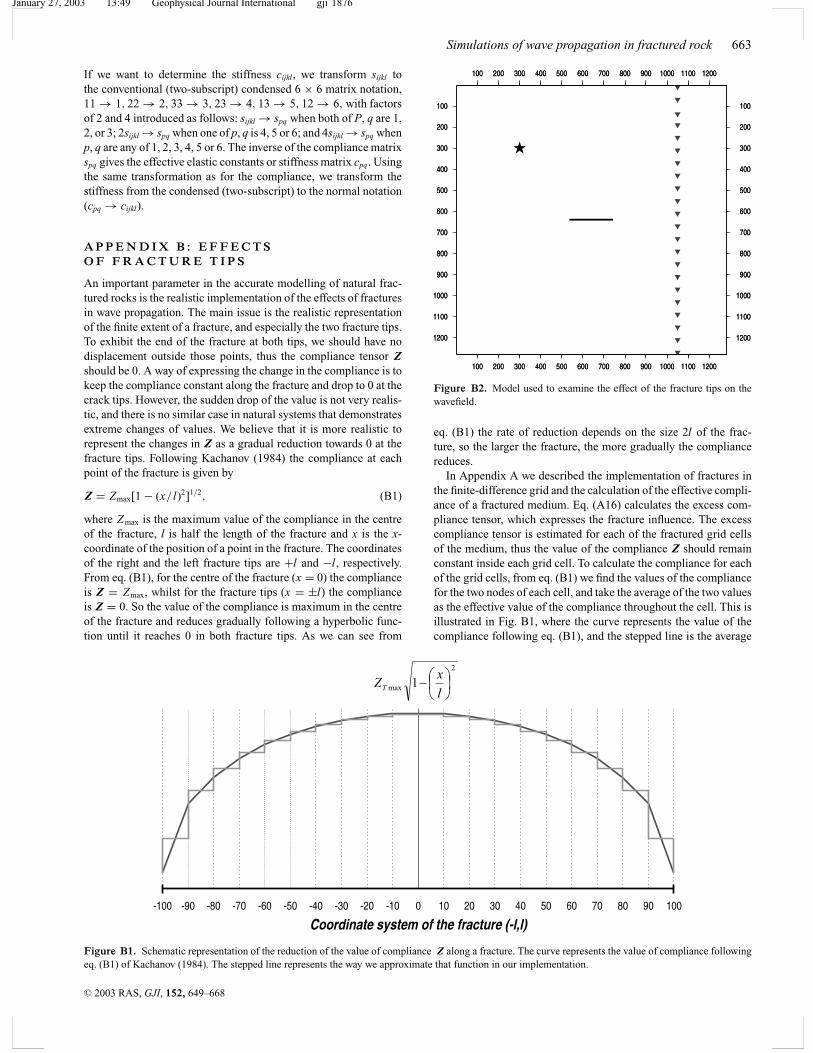
Figure B1. Schematic representation of the reduction of the value of compliance Z along a fracture. The curve represents the value of compliance followingeq. (B1) of Kachanov (1984). The stepped line represents the way we approximate that function in our implementation.

Figure B2. Model used to examine the effect of the fracture tips on thewavefield.

eq. (B1) the rate of reduction depends on the size 2l of the frac-ture, so the larger the fracture, the more gradually the compliancereduces.

In Appendix A we described the implementation of fractures inthe finite-difference grid and the calculation of the effective compli-ance of a fractured medium. Eq. (A16) calculates the excess com-pliance tensor, which expresses the fracture influence. The excesscompliance tensor is estimated for each of the fractured grid cellsof the medium, thus the value of the compliance Z should remainconstant inside each grid cell. To calculate the compliance for eachof the grid cells, from eq. (B1) we find the values of the compliancefor the two nodes of each cell, and take the average of the two valuesas the effective value of the compliance throughout the cell. This isillustrated in Fig. B1, where the curve represents the value of thecompliance following eq. (B1), and the stepped line is the average

C© 2003 RAS, GJI, 152, 649–668



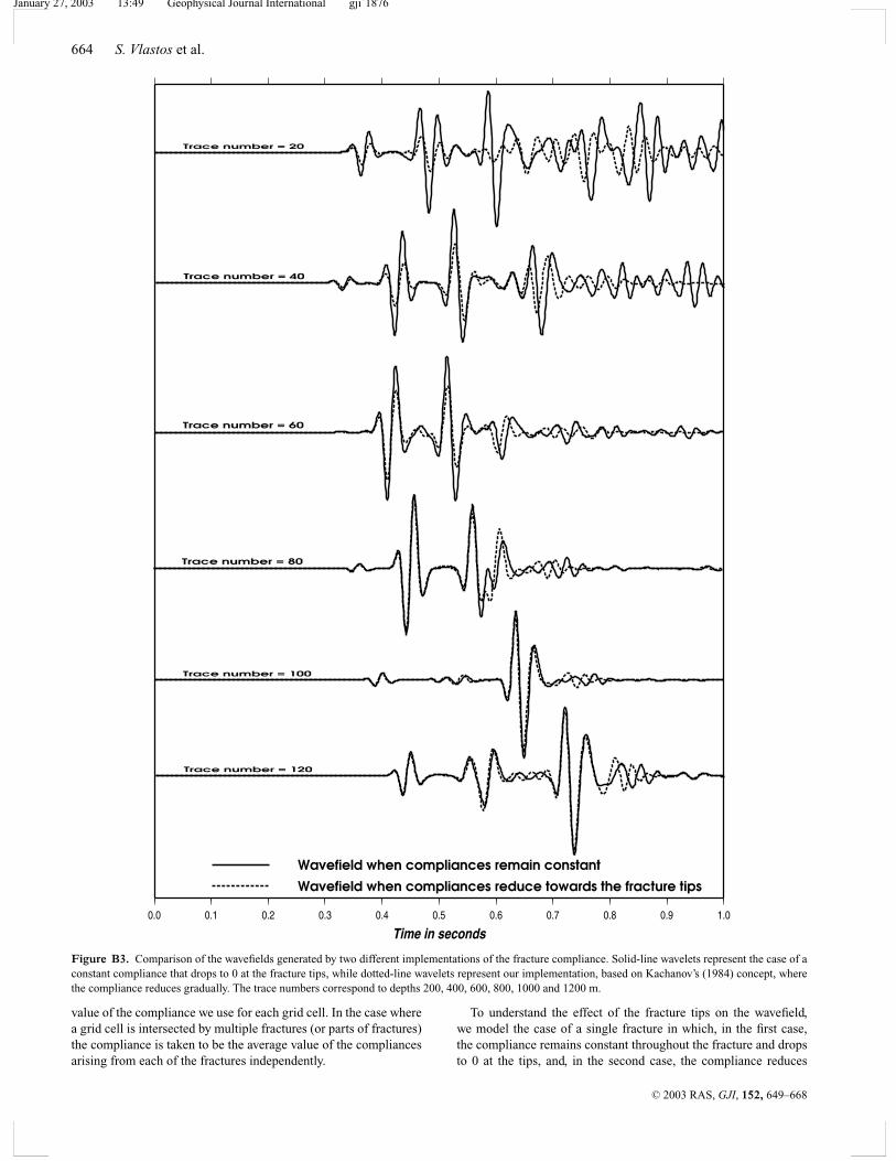
Figure B3. Comparison of the wavefields generated by two different implementations of the fracture compliance. Solid-line wavelets represent the case of aconstant compliance that drops to 0 at the fracture tips, while dotted-line wavelets represent our implementation, based on Kachanov’s (1984) concept, wherethe compliance reduces gradually. The trace numbers correspond to depths 200, 400, 600, 800, 1000 and 1200 m.

value of the compliance we use for each grid cell. In the case wherea grid cell is intersected by multiple fractures (or parts of fractures)the compliance is taken to be the average value of the compliancesarising from each of the fractures independently.

To understand the effect of the fracture tips on the wavefield,we model the case of a single fracture in which, in the first case,the compliance remains constant throughout the fracture and dropsto 0 at the tips, and, in the second case, the compliance reduces

C© 2003 RAS, GJI, 152, 649–668



following our implementation. The model we use is presented inFig. B2. For the two cases we compare the wavelets of a number oftraces and the results are presented in Fig. B3. The wavelets pre-sented in Fig. B3 do not include direct waves, because they are notaffected by the fracture tips, and so are identical. Also, the am-plitude of the wavelets is normalized between the several traces.However, the relative amplitude between the wavelets for each in-dividual trace remains accurate. From the comparison between thewavelets, we first observe that there is a time difference between theSS waves when we have constant compliance and when the com-pliances reduce gradually, with SS waves of the latter case beingslower. This may be a result of the sensitivity of S waves to changesof anisotropy. By changing the compliance from constant to vari-able, we effectively change the anisotropy, and this is only visiblein the SS wavelets. However, when we observe the wavelets fromtraces 100 and 120 we see that the time difference in the SS wavesdisappears. The waves observed at those receivers come from wavesdiffracted from the crack tips and from waves refracted at the frac-ture, in contrast to the rest of the receivers, where we have diffractedand reflected waves. Also, we can observe variations in the ampli-tude. In traces 20, 40 and 60, where the receivers are above thefracture, so we have reflected and diffracted waves, the amplitudeof the waves when the compliance is constant is higher than theamplitude when the compliance follows our implementation. Onthe other hand, in trace 80, when the waves are only diffracted, wehave opposite results. Finally, in traces 100 and 120, where we haverefracted and diffracted waves, the amplitudes seem to be almostidentical. We see that reflection and refraction are decisive factorsin the wavelet pattern. More research needs to be done on thesetopics to examine how they affect the waves.

Another parameter that we have not examined is the effect of thelength of the fracture. From eq. (B1) we can see that if we havea fracture of short length l then the reduction of the compliancewould be severe, whilst when the fracture is very large we willhave a very smooth reduction that can approximate the case of theconstant compliance throughout the fracture. This has to be testedby modelling various sizes of fractures and the respective wavelets,to find out at what point the approximation of constant complianceis satisfactory.

A P P E N D I X C : G E N E R A T I O NO F F R A C T U R E D I S T R I B U T I O N S

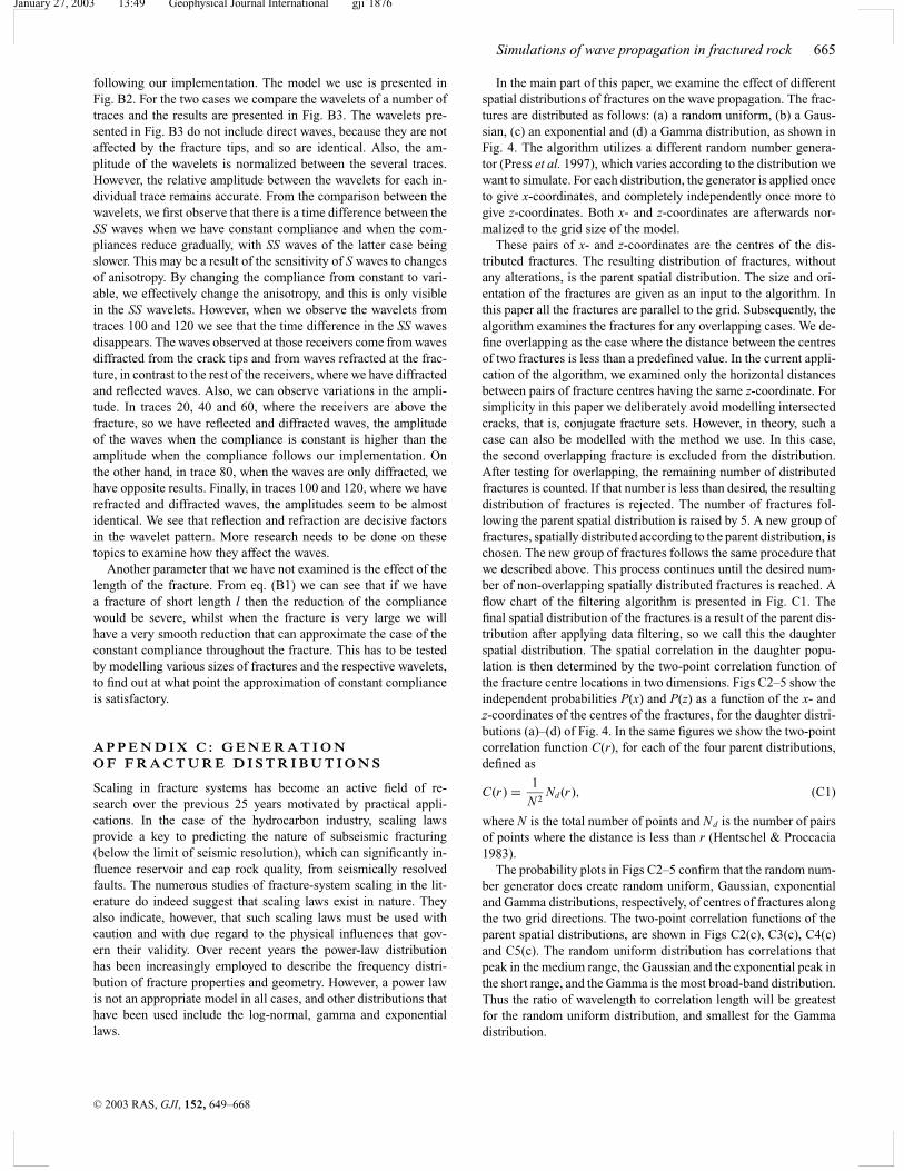
Scaling in fracture systems has become an active field of re-search over the previous 25 years motivated by practical appli-cations. In the case of the hydrocarbon industry, scaling lawsprovide a key to predicting the nature of subseismic fracturing(below the limit of seismic resolution), which can significantly in-fluence reservoir and cap rock quality, from seismically resolvedfaults. The numerous studies of fracture-system scaling in the lit-erature do indeed suggest that scaling laws exist in nature. Theyalso indicate, however, that such scaling laws must be used withcaution and with due regard to the physical influences that gov-ern their validity. Over recent years the power-law distributionhas been increasingly employed to describe the frequency distri-bution of fracture properties and geometry. However, a power lawis not an appropriate model in all cases, and other distributions thathave been used include the log-normal, gamma and exponentiallaws.

In the main part of this paper, we examine the effect of differentspatial distributions of fractures on the wave propagation. The frac-tures are distributed as follows: (a) a random uniform, (b) a Gaus-sian, (c) an exponential and (d) a Gamma distribution, as shown inFig. 4. The algorithm utilizes a different random number genera-tor (Press et al. 1997), which varies according to the distribution wewant to simulate. For each distribution, the generator is applied onceto give x-coordinates, and completely independently once more togive z-coordinates. Both x- and z-coordinates are afterwards nor-malized to the grid size of the model.

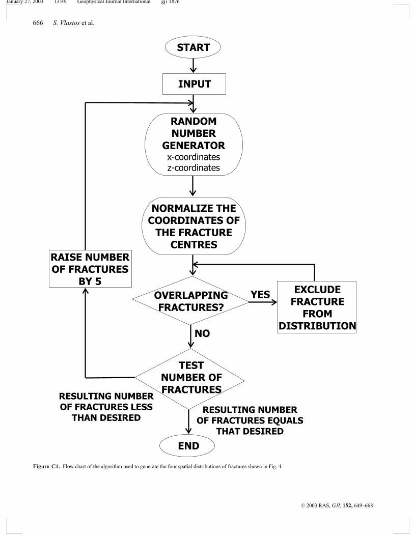
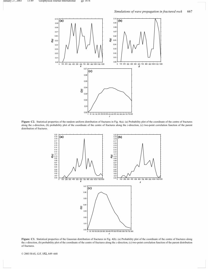
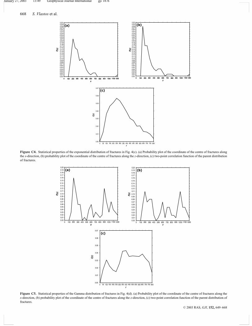
These pairs of x- and z-coordinates are the centres of the dis-tributed fractures. The resulting distribution of fractures, withoutany alterations, is the parent spatial distribution. The size and ori-entation of the fractures are given as an input to the algorithm. Inthis paper all the fractures are parallel to the grid. Subsequently, thealgorithm examines the fractures for any overlapping cases. We de-fine overlapping as the case where the distance between the centresof two fractures is less than a predefined value. In the current appli-cation of the algorithm, we examined only the horizontal distancesbetween pairs of fracture centres having the same z-coordinate. Forsimplicity in this paper we deliberately avoid modelling intersectedcracks, that is, conjugate fracture sets. However, in theory, such acase can also be modelled with the method we use. In this case,the second overlapping fracture is excluded from the distribution.After testing for overlapping, the remaining number of distributedfractures is counted. If that number is less than desired, the resultingdistribution of fractures is rejected. The number of fractures fol-lowing the parent spatial distribution is raised by 5. A new group offractures, spatially distributed according to the parent distribution, ischosen. The new group of fractures follows the same procedure thatwe described above. This process continues until the desired num-ber of non-overlapping spatially distributed fractures is reached. Aflow chart of the filtering algorithm is presented in Fig. C1. Thefinal spatial distribution of the fractures is a result of the parent dis-tribution after applying data filtering, so we call this the daughterspatial distribution. The spatial correlation in the daughter popu-lation is then determined by the two-point correlation function ofthe fracture centre locations in two dimensions. Figs C2–5 show theindependent probabilities P(x) and P(z) as a function of the x- andz-coordinates of the centres of the fractures, for the daughter distri-butions (a)–(d) of Fig. 4. In the same figures we show the two-pointcorrelation function C(r), for each of the four parent distributions,defined as

C(r ) = 1

N 2Nd (r ), (C1)

where N is the total number of points and Nd is the number of pairsof points where the distance is less than r (Hentschel & Proccacia1983).

The probability plots in Figs C2–5 confirm that the random num-ber generator does create random uniform, Gaussian, exponentialand Gamma distributions, respectively, of centres of fractures alongthe two grid directions. The two-point correlation functions of theparent spatial distributions, are shown in Figs C2(c), C3(c), C4(c)and C5(c). The random uniform distribution has correlations thatpeak in the medium range, the Gaussian and the exponential peak inthe short range, and the Gamma is the most broad-band distribution.Thus the ratio of wavelength to correlation length will be greatestfor the random uniform distribution, and smallest for the Gammadistribution.

C© 2003 RAS, GJI, 152, 649–668



Figure C1. Flow chart of the algorithm used to generate the four spatial distributions of fractures shown in Fig. 4.

C© 2003 RAS, GJI, 152, 649–668



Figure C2. Statistical properties of the random uniform distribution of fractures in Fig. 4(a). (a) Probability plot of the coordinate of the centre of fracturesalong the x-direction, (b) probability plot of the coordinate of the centre of fractures along the z-direction, (c) two-point correlation function of the parentdistribution of fractures.

Figure C3. Statistical properties of the Gaussian distribution of fractures in Fig. 4(b). (a) Probability plot of the coordinate of the centre of fractures alongthe x-direction, (b) probability plot of the coordinate of the centre of fractures along the z-direction, (c) two-point correlation function of the parent distributionof fractures.

C© 2003 RAS, GJI, 152, 649–668



Figure C4. Statistical properties of the exponential distribution of fractures in Fig. 4(c). (a) Probability plot of the coordinate of the centre of fractures alongthe x-direction, (b) probability plot of the coordinate of the centre of fractures along the z-direction, (c) two-point correlation function of the parent distributionof fractures.

Figure C5. Statistical properties of the Gamma distribution of fractures in Fig. 4(d). (a) Probability plot of the coordinate of the centre of fractures along thex-direction, (b) probability plot of the coordinate of the centre of fractures along the z-direction, (c) two-point correlation function of the parent distribution offractures.

C© 2003 RAS, GJI, 152, 649–668

numerical simulation of wave propagation in media with ... · numerical simulation of wave...

Documents