numerical solution of an inverse problem in a cell

Applied Mathematical Sciences, Vol. 6, 2012, no. 88, 4361 - 4380

Numerical Solution of an Inverse Problem

in a Cell Division Equation

Yves Emvudu

University of Yaounde 1, Department of mathematicsLaboratory of applied mathematics, P.O BOX 812, Yaounde, Cameroon

[email protected]

Dany Djeudeu

University of Yaounde 1, Department of mathematicsLaboratory of applied mathematics, P.O BOX 812, Yaounde, Cameroon

[email protected]

Abstract

The comprehension of the cellular division is fundamental in the study of many phe-nomenon like the growth of a tumor or of the cancer. Many models have been proposed todescribe the evolution of cell density: Model of Bell and Anderson in 1967 [1], model of Sinoand Streifer in 1967 and 1971. Many natural phenomenon have long been represented byordinary differential equations, but it is more realistic for cell division to consider the timeand size dependent equation. We obtain a system of hyperbolic partial differential equationnot easy to solve analytically. For the cell evolution, the problem in laboratories is generallyto find the cell division rate, from an experimental measure of cell density. The problemunder consideration is ill-posed in Hadamard’sense and we aim to determine the solution nu-merically. Of course, it is convenient to solve the direct problem before tracking the inverseone

Mathematics Subject Classification: 47J06, 35R30, 45K05, 47F05, 35L70

Keywords: inverse problem, structured population dynamics, cell division equation, eigen-value problem, Partial differential equation

1 Introduction

Most problems we encounter are direct problems in the sense that these problems are well-posedin Hadamard’sense. But many important problems to be solved are ill-posed in Hadamard’sense,like the problem of determining the cell division rate from an experimental data of cell density.Many author have explored the resolution of this problem: Benoit Perthame, George Zubelli,

4362 Y. Emvudu and D. Djeudeu

Marie Douminic [2], [4], [5], [6]. Here we will deeply explain and give an amelioration to thenumerical determination of the solution. We clearly pose the problem under consideration: Inlaboratories, it is generally just an experimental measure of cell density is available (experimentalmeasure of a stable distribution of cell density). From the experimental data, we show that itis possible to reconstruct the cell division rate. Let us notice how benefit it is to know the celldivision rate: in fact, it is possible to influence the cell division rate to control human heath.So, our paper is organized as followed: We firstly present the model and make some assumptionfor simplicity. Then we formulate an eigenvalue problem to be solved. Afterward, we use a fixedpoint theory to prove the existence of a stable distribution, an then we solve the direct problemnumerically and finally we attack the inverse problem. Numerical simulations are provided toillustrate our results

2 The model

Models for cell division equations are generally structured by one variable which is generallythe cell size. It could have been cell age. The original model had been presented by Bell andAnderson in 1967 [1]. The following model presented in [2] represents the evolution of celldensity:

⎧⎨⎩

∂n

∂t(t, x) +

∂

∂x[g(x)n(t, x)] + b(x)n(t, x) + μ(x)n(t, x) =

∫ 1

0

1σ2

β(x

σ, σ)dx

n(t, 0) = 0(1)

where

− n(t, x) represents the cell of size x at time t.

− β(x, σ) represents the division rate of the mother cells of size x into daughter cells of size σxand (1 − σ)x after mitosis. We have

β(y, σ) = β(y, 1 − σ) ∀σ

− g(x) denotes the individual growth rate of cells of size x.

− μ(x) denotes the death rate, or the chance (per time unit) that cells of size x dies

We choose simplicity and make the following assumptions:

• All cells of a micro-parasite class growth according to a deterministic rule.

• All cells after having reached a certain size (mother cell) divide into two part, just in two,giving birth to two identical daughter cells: it is called equal mitosis.

• Cell age does not influence the growth law and the preferred size of the division.

Numerical solution of an inverse problem 4363

• There is a negligible number of death during a normal growth.

• We assume g = 1. In fact, g(x) denotes the individual growth rate of cells of size x and wehave

dx

dt= g(x)

(assuming that there is not fission) and for g equal to a constant a, one finds

x(t) = x0 + at

where x0 is the initial size of cells and we obtain the linear model. We then choose a = 1just for simplicity. In fact, other cases are studied likewise.

Taking into account the above hypothesis, equation (1) becomes:{

∂n

∂x(t, x) +

∂n

∂t(t, x) + b(x)n(t, x) = 4b(2x)n(t,2x) x > 0, t ≥ 0

n(t, 0) = 0(2)

which is the partial differential equation of hyperbolic kind we are going to study.Solutions to the above equation could be determined using characteristic methods, but quan-

tities available for measure in a laboratory is a stable distribution N of cell density and theproblem is to determine the cell division rate numerically. The problem under consideration isill-posed in Hadamard’sense, so a regularization method is needed transform the initial probleminto a well-posed problem. It is necessary to formulate the problem to be solved clearly.

3 Existence of the stable distribution

Proposition 3.1 If we look for solutions of equation (2) in the form Ψ(t)N(t) (we separatevariables), then:

• N must satisfy an eigenvalue problem :

−dN

dx(x) − b(x)N(x) + 4b(2x)N(2x) = λN(x)

with λ =Ψ′

Ψconstant, independent of x and t

• Ψ(t) = eλt

• The adjoint equation of the eigenvalue problem is given by:{dΦdx

(x) − b(x)Φ(x) + 2b(x)Φ(x

2

)= λΦ(x), x ≥ 0

Φ(x) > 0, ∀x > 0(3)


Proof 3.1 Let’s set t, x ∈ R+ n(t, x)=Ψ(t)N(x). then,

∂n

∂x(t, x) +

∂n

∂t(t, x) + b(x)n(t, x) = 4b(2x)n(t,2x)

imply that:

Ψ′(t)N(x) + Ψ(t)dN

dx(x) + b(x)Ψ(t)N(x) = 4Ψ(t)b(2x)N(2x) (4)

dividing both members by Ψ(t) we obtain

Ψ′(t)Ψ(t)

N(x) +dN

dx(x) + b(x)N(x) = 4b(2x)N(2x)

which gives

Ψ′(t)Ψ(t)

=−dN

dx(x) − b(x)N(x) + 4b(2x)N(2x)

N(x)= λ, λ ∈ R

λ is an independent constant of t and of xΨ is then given by

Ψ(t) = ceλt, c ∈ R

Replacing Ψ by this value in equation (4), N must satisfy the following eigenvalue equation:

−dN

dx(x) − b(x)N(x) + 4b(2x)N(2x) = λN(x)

Considering the operator H:

H : L2(R+, dx) −→ L2(R+, dx)N �−→ HN,

where for x > 0,

HN(x) = −dN

dx(x) − b(x)N(x) + 4b(2x)N(2x).

Then, the adjoint operatorA∗ is defined on the same spaces. And for x > 0 by

H∗Φ(x) =dΦdx

(x) − b(x)Φ(x) + 2b(x)Φ(x

2

).

The parameter λ which is the dominant eigenvalue is generally called Malthus parameter ([6])If we add the condition of normalization to the eigenvalue equation, we obtain the following

equation: ⎧⎪⎪⎪⎪⎪⎨⎪⎪⎪⎪⎪⎩

−dN

dx(x) − b(x)N(x) + 4b(2x)N(2x) = λN(x), x ≥ 0

N(x) > 0, ∀x > 0 ,N(0) = 0∫ +∞

0N(x)dx = 1

(5)


3.1 Analysis of fixed points

A fixed point of system (2) is given by:

n∗(x) = 4∫ 2x

0b(u)n∗(u)e−

� u2

x b(σ)dσdu (6)

We define the following operator:

(Φ)(Ψ)(x) = 4∫ A

01[0,2x](u)b(u)Ψ(u)e−

� u2

xb(σ)dσdu

=∫ A

0Ψ(u)λ(x, u)du

Ψ ∈ E = L1([0,A])We study the fixed points of Φ using the theory of positive operators defined on a cone in a

Banach space.with

λ(x, u) = 41[0,2x](u)b(u)e−� u

2x b(σ)dσ

where A is the maximal size. Each fixed point of Φ in the positive cone is a cell density thatsatisfies (6)

Proposition 3.2 Let E = L1([0,A]) with the positive cone E+ = {Ψ ∈ E : Ψ ≥ 0, a.e.}, andlet de

There exists a unique non zero positive fixed point of the operator Φ

Proof 3.2 For the proof of this proposition, we will prove that the operator Φ is compact, Nonsupporting,

Lemma 3.1 the following assumptions are held:

1. λ ∈ L+∞+ (([0,A] × [0, A]))

2. limh−→0

∫ A0 |λ(x + h, ξ) − λ(x, ξ)|dx = 0, where λ is extended by λ(x, ξ) = 0 for x, ξ ∈

] −∞, A[∪]A,+∞[

3. There exist numbers α with A > α > 0 and ε > 0 such that λ(x, ξ) ≥ ε for almost all(x, ξ) ∈]0, A[×]A − α,A[

Proof 3.3 the proof of the above lemma comes from the definition of λ

Lemma 3.2 Under the assumptions of the above lemma, the operator Φ : E −→ E is nonsupporting and compact.


Proof 3.4 Let us define the positive linear functional f0 ∈ E∗+ by

〈f0,Ψ〉 =∫ A

0s(u)bm exp(−

∫ u2

xb(σ)dσ)Ψ(u)du,Ψ ∈ E (7)

wherethere ∃ bm > 0 et bM < +∞ such that bm < b(x) < bM ∀ x > 0.the function s(ξ) is defined as s(ξ) = 0, ξ ∈ [0, A − α]; s(ξ) = ε, ε ∈]A − α,A[. Hence,

λ(x, ξ) ≥ s(ξ) for almost all (x, ξ) ∈ [0, A] × [0, A]. It is easy to see that the functional f0 isstrictly positive and

Φn+1Ψ ≥ 〈f0,Ψ〉ε, ε = 1 ∈ E+,Ψ ∈ E+ (8)

Then for any integer n we have

ΦΨ ≥ 〈f0,Ψ〉ε, ε = 1 ∈ E+,Ψ ∈ E+ (9)

Therefore we obtain 〈F,ΦnΨ〉 > 0, n ≥ 0 for every pair Ψ ∈ E+/{0}, F ∈ E∗+/{0}, that is,

Φ is nonsupporting. Next, it is easy to see that the operator Φ is compact.

In [3] the following lemma was proved:

Lemma 3.3 Let r(Φ) be the spectral radius of the operator Φ. Then the following holds:

1. If r(Φ) ≤ 1, The only nonnegative solution of the equation ΦΨ = Ψ is the trivial solutionΨ = 0

2. If r(Φ) > 1, the equation ΦΨ = Ψ has at least one non-zero positive solution.

Remark 3.1 For uniqueness, it has also been proved that if λ(x, y) can be factorized and ma-jored by u(x)v(y) (which is called the proportionate mixing assumption), it is easily seen thatthere always exists a unique non trivial steady state under the condition

r(T ) =∫ A

0λT (σ, σ)dσ > 1 (10)

with

T (Ψ)(x) =∫ A

0Ψ(u)λT (x, u)du

Ψ ∈ E = L1([0,A]) with λT (x, y) = u(x)v(y)

In this case, u(x) is the eigenvector of the operator T corresponding to the spectral radius r(T ).In our case, it is easy to see that λ(x, y) ≤ λT (x, y) and λT (x, y) satisfy the proportionate mixingassumption.


4 Numerical solution of the cell division equation

To solve the problem numerically, we have to ensure that the problem is well posed in Hadamard’sense.Else, the numerical solution would have nothing in common with the real data. The followingtheorems had been proved in [5]

Theorem 4.1 (Existence and uniqueness of solution)Let us admit the following hypothesis:

• b ∈ C(R+)

• ∃ bm > 0 et bM < +∞ such that bm < b(x) < bM ∀ x > 0.

Then there exists a unique (λ,N,Φ) to the equations (5) and (3) with Φ, N ∈ C1(R+) suchthat N positive {

bm ≤ λ ≤ bMc

(1 + x)k≤ Φ(x) ≤ C(1 + xk)

where c, C and k are 3 positive constant such that

2kbm > bM

N and its derivative vanish at 0 and +∞

Theorem 4.2 Let us consider the above hypothesis:

• b ∈ C(R+)

• ∃ bm > 0 et bM < +∞ tel que bm < b(x) < bM ∀ x > 0,

The application

Γ : b −→ (λ,N)

is

1. continue en b de L∞(R+) in [bm, bM ]×L1 ∩L∞(R+) under the weak topology of L∞(R+)

2. Locally lipscht-continuous in b under the strong topology of L2(R+) in [bm, bM ] × L2(R+)

3. of class C1 from L2(R+) to [bm, bM ] × L2(R+)

We are now going to solve the general problem (Equation (1)) numerically. Then we willsolve the eigenvalue problem and then compare the numerical result and confirm the long termconvergence of the cell density to a stable distribution.


4.1 General equation

We solve our equation on the rectangle [0;T ] × [0;L]The closed intervalle [0;L] is discretised in m + 1 noddles xi for i = 0, ...,m with a regular

amplitude. Let us denote Δx the time amplitude. The same is done with the time intervalleand we denote Δt the time amplitude ([0, T ] is divided into n points ). Let’s nk

i The cell densityat xi = iΔx at time tk = kΔt. We use the following scheme

(1 + β + Δtbi)nk+1i − βnk+1

i−1 − 4Δtb2ink+12i = nk

i 1 ≤ i ≤ m (11)

with β =Δt

Δxwhich is consistent, stable without condition. We then obtain a linear system to be solved.

We just want to stress on the method we used to store the matrix of the linear system in orderto optimize the memory space: the storage method of Moorse whose principle is: This datastructure has three tables with the following functions:

1. A table containing the non-zero element values of the matrix, given line by line. We denotethis table AA. Its dimension (length) is nz, representing the number of non-zero elementsof the matrix B of the linear system

2. A table of integer containing the index of colon corresponding to the elements of table byAA. We denote this table by J

3. A table of integer containing a pointer on the position where each line begins in the tableAA and J . Its i-th element, I(i) will thus contain for i = 1, ...,m, the posit ion wherebegins the i-th line in tables AA and J . It s dimension will be m + 1 with a conventionthat I(m + 1) = nz + 1. ie the address of the beginning of a fictive (n + 1) − th line intables AA and J .

4.2 Numerical solution of the eigenvalue problem

The problem under consideration is the eigenvalue problem that we solve on the interval [0, L]:AX = λX .After discretization we obtain AhYh = λhYh.

The direct problem being well posed, let us solve it by a stable numerical method.we solve the problem on the finite interval [0, L]

let us consider equation (5) on [0, L] and assume that the cell density is known and verify thefollowing conditions:

• b ∈ C(R+)

• ∃ bm > 0 et bM < +∞ tel que bm < b(x) < bM ∀ x > 0.


Let ([xi, xi+1])0≤i≤m a subdivision of the interval [0, L] in m interval of same amplitude

h =L

m. xi+1 = xi + h, i = 0 . . . m. we obtain the following discreet equation:

{Ni − Ni−1

h+ (λ + bi)Ni + 4b2iN2i12i≤L

2= λiNi, 1 ≤ i ≤ L

hN0 = 0

(12)

with Ni = N(xi)This equation leads us to the following equation:

AhYh = λhYh (13)

with Ah = (ai,j), i, j ∈ {1 . . . m} defined as followed:⎧⎪⎪⎪⎪⎪⎨⎪⎪⎪⎪⎪⎩

ai,i = −1h− bi, i = 1 . . . m;

ai,i−1 =1h

, i = 2 . . . m;

ai,2i = 4b2i, i = 1 . . . [m2 ];ai,j = 0, si j �= i, 2i, i − 1.

Then we use a MATLAB function to determine the dominant eigenvalue that the eigenvectoris the stable distribution.

4.3 Long term behavior of the evolution equation

We will draw figures that compare the solution of the evolution equation and the numericalsolution to the eigenvalue problem

4.3.1 Observation and Interpretation of numerical results

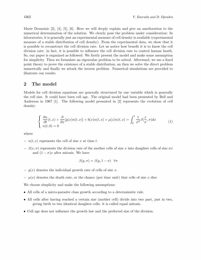
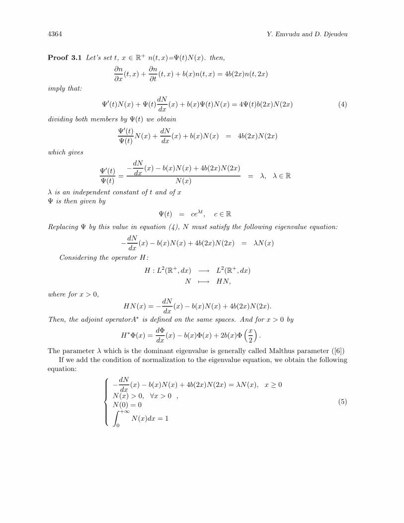
Figure (4.3),(4.3), (4.3),(4.3) represent the approximated solution to the direct problem: de-termination of the cell density for the non-perturbed division rate b = 1. This passes throughthe resolution of an eigenvalue equation that we have represented the solution. Observing thecurve representing the surface of density, we notice that after a certain time T hight enough,the surface takes a stable form that we have also represented: It is the said stable distribution.We also notice that n(T, .) has the same form with N, solution to the eigenvalue equation. Therepresentation of both quantities in the same frame permits to verify that n(T, .) is a multipleof N . This illustrate the said convergence of cell density to a stable distribution. This is animportant result: In fact, in laboratories the quantity available for measure is the stable dis-tribution. Or, mathematically we can solve the eigenvalue equation and effectively deduce thestable distribution.

Figure (4.3),(4.3),(4.3),(4.3) represent the approximated solution of the said direct problemfor a random perturbation of the cell division rate. The curve obtained are practically identic tothose without perturbation: A small perturbation of data has not greatly changed the solution.


[surface of cell density for b=1]

[Long term behavior of the cell density for b=1]


[Solution of the eigenvalue problem for b=1]

[Comparison of solutions for b=1]

Figure 1: Approximated cell density for the non perturbed division rate


[surface of cell density for b=1+0,001*max(rand(1,5))/norm(rand(1,5))]

[Long term behavior of the cell density for b=1+0,001*max(rand(1,5))/norm(rand(1,5))]


[Eigenvector for b=1+0,001*max(rand(1,5))/norm(rand(1,5))]

[Comparison of solutions for b=1+0,001*max(rand(1,5))/norm(rand(1,5))]

Figure 2: Approximated cell density for a random perturbation of division rate


[surface of cell density for b=1+exp(−8(x − 2)2)]

[Long term behavior of the cell density for b=1+exp(−8(x − 2)2)]


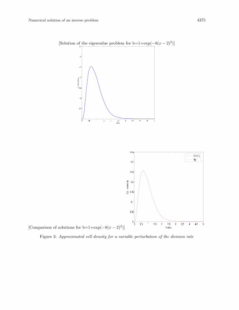
[Solution of the eigenvalue problem for b=1+exp(−8(x − 2)2)]

[Comparison of solutions for b=1+exp(−8(x − 2)2)]

Figure 3: Approximated cell density for a variable perturbation of the division rate


Figure (4.3), (4.3), (4.3), (4.3) represents also the above quantities, with a variable pertur-bation of cell division rate. the conclusion is the same. This illustrate the well-posedness of thedirect problem: the problem of determining the cell density from an experimental measure ofcell division rate.

5 Numerical solution of the inverse problem

The inverse problem we have said consists of determining the division rate b from a noisy measureof the stable distribution (λ,N). we have to inverse the application

Γ : b −→ (λ,N) (14)

in suitable spaces, where b, N , λ are linked by the following eigenvalue equation:⎧⎪⎪⎪⎪⎪⎨⎪⎪⎪⎪⎪⎩

−dN

dx(x) − b(x)N(x) + 4b(2x)N(2x) = λN(x), x ≥ 0

N(x) > 0, ∀x > 0 ,N(0) = 0∫ +∞

0N(x)dx = 1

(15)

It had been shown in [4] that

Γ−1 : [bm, bM ] × L1 ∩ L∞(R+) −→ L∞(R+)(λ,N) −→ b

is not continuous. Thus, the problem under consideration is ill-posed in Hadamard’sense. Soregularization is needed. It was also proved [5] that

⎧⎨⎩ α

d(bαN)dy

(y) + 4bα(y)N(y) = bα

(y

2

)N

(y

2

)+ λN

(y

2

)+ 2

dN

dy

(y

2

), y > 0

bαN(0) = 0(16)

(where 0 < α < 1 is the regularization parameter)is a well-posed equation in Hadamard’sense. And the solution bα of the above equation is

closed to the solution b of equation (5). We are going to concentrate on numerical simulations.Before simulations, we notice that instead of observing the stable distribution (λ,N), it is a

noisy Nε that is observed, and we deduce from the combination of equation (16) and (5) that

λα,ε =

∫ +∞

0Nεdx∫ +∞

0xNεdx +

α

4

∫ +∞

0Nεdx

(17)


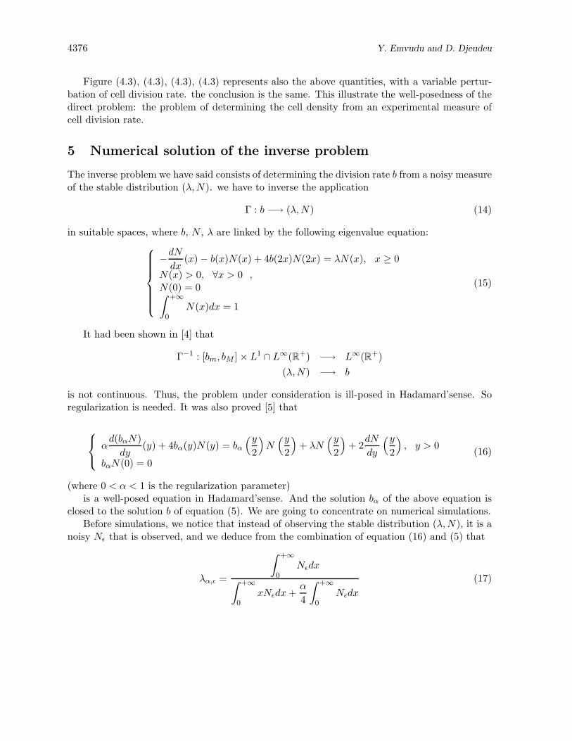
[Product bN for b=1]

Before presenting numerical results, we note that we firstly represent the product bN beforededucing b. We notice that data we use to solve the inverse problem are the results obtained fromthe direct problem and we tries to reconstruct the initial data: with known division rate, we founda stable distribution numerically, we then use the stable distribution obtained numerically toreconstruct the initial division rate. We notice that there are two major source of error: The errorfrom the experimental measure of the stable distribution and the error due to regularization.

5.0.2 Observations and interpretation

Figure (5) and (5) reconstruct the cell division rate b used to solve the direct problem. Takingthe regularization parameter near to 0, we notice that the product bN is practically equal to N .Thus, b is almost 1 and the reconstruction is very good (Almost perfect). It is in this mannerthat in laboratories, a single observation of the stable distribution of cell density enables toreconstruct the cell division rate satisfactorily.

We have the same conclusions with figure (5) and (5) since the rate to reconstruct is near 1.

6 Conclusion

It has been question to solve a ill-posed problem in Hadamard’sense numerically: determinationof cell division from a noisy data of a stable distribution of cell density. It has been necessary toconsider the direct problem before numerical solution to the inverse problem to prove that thereconstruction of cell division rate could be obtained from an experimental data of cell density.Numerical solutions obtained are quite satisfactory, noting both source of error.


[Reconstruction of the division rate for b=1, α = 0.001]

[Product bN for b=1+0,001*max(rand(1,5))/norm(rand(1,5))]


[Reconstruction of the division rate for b=1+0,001*max(rand(1,5))/norm(rand(1,5)),

α = 0.0001]

Figure 4: Reconstruction of the cell division rate

7 Discussion

The model studied in this paper is a simplified model with the hypothesis we made. Also, theregularization used here (In the same sense as Tikhonov method is quite good, but could beameliorated. We propose ourselves in the near future to study the general model of cell densityand propose a new regularization method for the inverse problem). We have not stressed on theregularization parameter, but the regularization plays a urge role on the numerical solution. Inour next work in the near future we shall attack that problem.

References

[1] G.I.Bell and E.C.Anderson, cell growth and division, I.A mathematical model withapplications to cell volume distribution in mammalian suspension cultures. Biophys.J.7(1967),329 − 351; 8(1963),431 − 444.

[2] Philipe Michel, Stephane Misler, Benoit Perthame: General entropy equations for structuredpopulation models and scattering, C.R.Acad.Sc.paris, Ser.I 338(2004)697 − 702.

[3] H. Inaba: Threshold and stability results for an age-structured epidemic model,J.Math.Biol.(1990) 28 :411 − 434

[4] Benoit Perthame, Jorge Zubelli, On the inverse problem for a size-structured populationmodel, inverse problems 23(2007) 1037 − 1052.


[5] Marie Douminic, Benoit perthame, Jorge Zubelli, Numerical solution of an inverse problemin size-structured population dynamics. hal-00327151, version 1-7 Oct 2008.

[6] Benoit perthame, Lenya Ryzhik, Exponential decay for the fragmentation or cell divisionequation, October 2004

[7] Bernd Hofmann, Mathematik inverser probleme, B.G. Teubner Stuttgart Leipzig, 1999.

Received: April, 2012

numerical solution of an inverse problem in a cell

Documents