Numerical Solution of the Hamilton-Jacobi-Bellman Formulation

for Continuous Time Mean Variance Asset Allocation ∗

J. Wang †, P.A. Forsyth ‡

December 20, 2008

Abstract

We solve the optimal asset allocation problem using a mean variance approach. The originalmean variance optimization problem can be embedded into a class of auxiliary stochastic Linear-Quadratic (LQ) problems using the method in (Zhou and Li, 2000; Li and Ng, 2000). We usea finite difference method with fully implicit timestepping to solve the resulting non-linearHamilton-Jacobi-Bellman (HJB) PDE, and present the solutions in terms of an efficient frontierand an optimal asset allocation strategy. The numerical scheme satisfies sufficient conditionsto ensure convergence to the viscosity solution of the HJB PDE. We handle various constraintson the optimal policy. Numerical tests indicate that realistic constraints can have a dramaticeffect on the optimal policy compared to the unconstrained solution.

Keywords: Optimal control, mean variance tradeoff, HJB equation, viscosity solution

JEL Classification: C63, G11

AMS Classification 65N06, 93C20

1 Introduction

Continuous time mean variance asset allocation has received considerable attention over the years(Zhou and Li, 2000; Li and Ng, 2000; Nguyen and Portrai, 2002; Leippold et al., 2004; Bielecki et al.,2005). Financial applications include hedging futures (Duffie and Richardson, 1991), insurance(Chiu and Li, 2006; Wang et al., 2007), pension asset allocation (Gerrard et al., 2004; Hojgaardand Vigna, 2007) and optimal execution of trades (Lorenz and Almgren, 2007). In its simplestformulation, an investor can choose to invest in a risk-free bond or a risky asset, and can dynamicallyalter the proportion of wealth invested in each asset, in order to achieve a mean variance efficientresult.

∗This work was supported by a grant from Tata Consultancy Services and the Natural Sciences and EngineeringResearch Council of Canada.

†David R. Cheriton School of Computer Science, University of Waterloo, Waterloo ON, Canada N2L 3G1 e-mail:

j27wang@uwaterloo.ca‡David R. Cheriton School of Computer Science, University of Waterloo, Waterloo ON, Canada N2L 3G1 e-mail:

paforsyt@uwaterloo.ca

1

The continuous time mean variance problem does not lend itself easily to a dynamic program-ming formulation. There are have been two main approaches to this problem. The original meanvariance optimal control problem can be embedded into a class of auxiliary stochastic Linear-Quadratic (LQ) problems, which can then be solved in terms of dynamic programming (Zhouand Li, 2000; Li and Ng, 2000). Alternatively, Martingale techniques can be used (Bielecki et al.,2005). In the case of the LQ method, previous papers use analytic techniques to solve the nonlinearHamilton-Jacobi-Bellman (HJB) PDE for special cases. In order to obtain analytic solutions, theauthors typically make assumptions which allow for the possibility of unbounded borrowing andinfinite negative wealth (bankruptcy). However, some analytic solutions have been developed forhandling specific constraints: no stock shorting (Li et al., 2002) (but shorting the bond is stillallowed) and the no bankruptcy case (Bielecki et al., 2005) (but again allowing for shorting thebond).

Although investment policy based on mean variance optimization has its critics, an advantageof this approach compared to power-law or exponential utility maximization is that the results canbe easily interpreted in terms of an efficient frontier.

The objective of this paper is to develop a numerical method for solving the continuous timemean variance optimal asset allocation problem. We will use a fully numerical scheme based onsolving the HJB equation resulting from the LQ formulation. Our scheme can easily handle anytype of constraint (e.g. non-negative wealth, no shorting of stocks, margin requirements).

Although the methods developed in this paper can be applied to any asset allocation problem,such as those discussed in (Nguyen and Portrai, 2002; Bielecki et al., 2005; Chiu and Li, 2006; Wanget al., 2007) we will focus on asset allocation problems which are relevant to defined contributionpension plans as discussed in (Hojgaard and Vigna, 2007; Cairns et al., 2006). In (Hojgaard andVigna, 2007), the objective is to determine the mean variance efficient strategy in terms of finalwealth. In (Cairns et al., 2006), the pension plan model includes a stochastic salary component. In(Cairns et al., 2006), the problem was formulated in terms of maximizing the utility of the wealth-to-income ratio. Here, we consider the same model, but solve for the optimal continuous timemean variance efficient frontier. Note that by setting the contribution rate to zero, the pensionplan problem reduces to the classical continuous time (multi-period) portfolio selection problem(Zhou and Li, 2000; Li and Ng, 2000; Li et al., 2002; Bielecki et al., 2005; Li and Zhou, 2006).

The main results of this paper are

• Based on the methods in (Forsyth and Labahn, 2008; Wang and Forsyth, 2008), we develop afully implicit method for solving the nonlinear HJB PDE, which arises in the LQ formulationof the mean variance problem. Under the assumption that the HJB equation satisfies a strongcomparison property, our methods are guaranteed to converge to the viscosity solution of theHJB equation. In addition, the policy iteration scheme used to solve the nonlinear algebraicequations at each timestep is globally convergent. Note that an explicit method would havetimestep restrictions due to stability considerations. In the case of an unbounded control, themaximum stable timestep would be difficult to estimate. This problem does not arise if animplicit method is used.

• By solving the HJB PDE and a related linear PDE, we develop a numerical method forconstructing the mean variance efficient frontier (in continuous time). Any type of constraintcan be applied to the investment policy.

2

• We pay particular attention to handling various constraints on the optimal policy. In partic-ular, in order to compare the numerical solution with the known analytic solution in specialcases, it is necessary to allow for negative wealth and unbounded controls. This requirescareful attention to the grid construction and form of the control as the mesh and timestepsshrink to zero.

• From a practical point of view, we observe that the addition of realistic constraints cancompletely alter some of the properties of the mean variance solution compared to the un-constrained control case (Li and Zhou, 2006).

We should point out here that the optimal mean variance strategy in (Zhou and Li, 2000; Li andNg, 2000; Nguyen and Portrai, 2002; Leippold et al., 2004; Bielecki et al., 2005; Chiu and Li, 2006;Wang et al., 2007; Hojgaard and Vigna, 2007) is the pre-commitment strategy, i.e. once the initialstrategy has been determined (as a function of the state variables) at the initial time, the investorcommits to this strategy, even if the the mean variance policy, computed at a later time woulddiffer from the pre-commitment strategy. This contrasts with the time-consistent policy wherebythe investor optimizes the mean variance tradeoff at each instant in time, assuming optimal meanvariance strategies at each later instant. The subtle distinction between these two approachesis discussed in (Basak and Chabakauri, 2007). We note that the efficient frontier for the pre-commitment strategy must always lie above the efficient frontier for the time-consistent strategy.However, there is some economic controversy about the meaning of these two approaches. We willfocus on the pre-commitment policy in this paper, leaving the time-consistent problem for futurework.

2 Mean Variance Efficient Wealth Case

We first consider the problem of determining the mean variance efficient strategy in terms of theinvestor’s final wealth. We will refer to this problem in the following as the wealth case. This willallow an explanation of the basic approach for construction of the efficient frontier, without unduealgebraic complication. For certain special cases, there are also some analytic solutions available(Hojgaard and Vigna, 2007) for this problem. This will enable us to compare with the numericalsolution.

Suppose there are two assets in the market: one is risk free (e.g. a government bond) and theother is risky (e.g. a stock index). The risky asset S follows the stochastic process

dS = (r + ξ1σ1)S dt + σ1S dZ1 , (2.1)

where dZ1 is the increment of a Wiener process, σ1 is volatility, r is the interest rate, ξ1 is themarket price of risk (or Sharpe ratio) and the stock drift rate can then be defined as µS = r + ξ1σ1.Suppose that the plan member continuously pays into the pension plan at a constant contributionrate π in the unit time. Let W (t) denote the wealth accumulated in the pension plan at time t,let p denote the proportion of this wealth invested in the risky asset S, and let (1− p) denote thefraction of wealth invested in the risk free asset. Then,

dW = [(r + pξ1σ1)W + π]dt + pσ1WdZ1 , (2.2)W (t = 0) = w0 ≥ 0 .

3

We will use the following notation throughout this paper,

E[·] : expectation operator,V ar[·] : variance operator,Std[·] : standard deviation operator,

Et[·], V art[·] or Stdt[·] : E[·], V ar[·] or Std[·] when sitting at time t,

Etp[·], V art

p[·] or Stdtp[·] : E[·|p], V ar[·|p] or Std[·|p] when sitting at time t. (2.3)

Let WT = W (t = T ). Given a risk level (defined as the variance of terminal wealth V art=0[WT ]),an investor desires her expected terminal wealth Et=0[WT ] to be as large as possible. Equiva-lently, given an expected terminal wealth Et=0[XT ], she wishes the risk V art=0[WT ] to be as smallas possible. Using a Lagrange multiplier, the control problem is then to determine the controlp(t, W (t) = w), where W (t) is the path of W given the control p(t, w), such that p(t, w) maximizes

maxp(t,w)

(Et=0[WT ]− λV art=0[WT ]), (2.4)

subject to stochastic process (2.2), and where λ > 0 is a given Lagrange multiplier. The multiplierλ can be interpreted as a coefficient of risk aversion. Varying λ ∈ [0,∞) allows us to draw anefficient frontier. Note we have emphasized here that the expectations in equation (2.4) are as seenat t = 0 (the pre-commitment solution).

We would like to use dynamic programming to determine the efficient frontier, given by equation(2.4). However, the presence of the variance term causes some difficulty. This can be avoided withthe help of the following result (Zhou and Li, 2000; Li and Ng, 2000).

Theorem 2.1 If p∗(t, w) is the optimal control of problem (2.4), then p∗(t, w) is also the optimalcontrol of problem,

maxp(t,w)

Et=0[µWT − λW 2T ] (2.5)

whereµ = 1 + 2λEt=0

p∗ [WT ] . (2.6)

Proof . See (Zhou and Li, 2000; Li and Ng, 2000). �

2.1 Reduction to an LQ Problem

Let,

D := the set of all admissible wealth W (t), for 0 ≤ t ≤ T ;P := the set of all admissible controls p(t, w), for 0 ≤ t ≤ T and w ∈ D. (2.7)

Let γ = µλ , then from equation (2.6),

γ =1λ

+ 2Et=0p∗ [WT ] . (2.8)

4

For a fixed γ, with λ > 0, equation (2.5) is equivalent to

minp(t,w)

Et=0[(WT −γ

2)2] . (2.9)

Let J(t, w, p) = E[(WT − γ2 )2|W (t) = w], where W (t) is the path of W given the asset allocation

strategy p = p(t, w). We define

V (w, τ) = infp∈P

E[(WT −γ

2)2|W (t = T − τ) = w] = inf

p∈PJ(t = T − τ, w, p) . (2.10)

where τ = T − t. Then using equation (2.2) and Ito’s Lemma, we have that V (w, τ) satisfies theHJB equation

Vτ = infp∈P

{µpwVw +

12(σp

w)2Vww} ; w ∈ D, (2.11)

with terminal condition

V (w, τ = 0) = (w − γ

2)2 , (2.12)

and where

µpw = π + w(r + pσ1ξ1)

(σpw)2 = (pσ1w)2 . (2.13)

In order to trace out the efficient frontier solution of problem (2.4), we proceed in the followingway. Pick an arbitrary value of γ and solve problem (2.5), which determines the optimal controlp∗(t, w). We also need to determine Et=0

p∗ [WT ].Let U = U(w, τ) = E[WT |W (t = T − τ) = w, p(t = T − τ, w) = p∗(t = T − τ, w)] . Then U is

given from the solution to

Uτ = {µpwUw +

12(σp

w)2Uww}p(t=T−τ,w)=p∗(t=T−τ,w) ; w ∈ D , (2.14)

with the payoffU(w, τ = 0) = w . (2.15)

Since the most costly part of the solution of equation (2.11) is the determination of the optimalcontrol p∗, solution of equation (2.14) is very inexpensive, since p∗ is known.

Note that Et=0p∗ [const.] = const.. Assume that W = w0 at t = 0. Then

V (w0, τ = T ) = Et=0p∗ [W 2

T ]− γEt=0p∗ [WT ] +

γ2

4,

U(w0, τ = T ) = Et=0p∗ [WT ] . (2.16)

Assuming V (w0, τ = 0), U(w0, τ = 0) are known, then for a given γ, we can then compute the pair(V art=0

p∗ [WT ], Et=0p∗ [WT ]) from V art=0

p∗ [WT ] = Et=0p∗ [W 2

T ]− (Et=0p∗ [WT ])2.

5

From equation (2.8) we have that

12λ

=γ

2− Et=0

p∗ [WT ] , (2.17)

which then determines the value of λ in problem (2.4). In other words, we have determined thepair (Stdt=0

p∗ [WT ], Et=0p∗ [WT ]) for the optimal control p∗ which solves problem (2.4), with the value

of λ given from equation (2.17).We then pick another value of γ, and obtain another point on the efficient frontier for another

value of λ, and so on. Note that we are effectively using the parameter γ to trace out the efficientfrontier. Since λ > 0, we must have (from equation (2.17))

γ

2− Et=0

p∗ [WT ] > 0 (2.18)

for a valid point on the frontier.

Remark 2.1 Note that the set of solutions for the original problem (2.4) is a subset of the setof controls for the auxiliary problem (2.5). As a result, the pair (Stdt=0

p∗ [WT ], Et=0p∗ [WT ]) from the

optimal strategy of problem (2.5) may not be a point on the efficient frontier for problem (2.4). Tofind the efficient frontier for the original optimization problem (2.4), we construct an upper convexhull from the candidate points (Stdt=0

p∗ [WT ], Et=0p∗ [WT ]) obtained by varying γ.

Remark 2.2 If we allow an unbounded control set P = (−∞,+∞), then the total wealth canbecome negative (i.e. bankruptcy is allowed). In this case D = (−∞,+∞). If the control set P isbounded, i.e. P = [pmin, pmax], then negative wealth is not possible, in which case D = [0,+∞). Wecan also have pmax → +∞, but prohibit negative wealth, in which case D = [0,+∞) as well.

2.2 Localization

Let,

D := a finite computational domain which approximates the set D. (2.19)

In order to solve the PDEs (2.11), (2.14) we need to use a finite computational domain, D =[wmin, wmax]. When w → ±∞, we assume that

V (w → ±∞, τ) ' H1(τ)w2 + H2(τ)w + H3(τ) ,

U(w → ±∞, τ) ' J1(τ)w + J2(τ) . (2.20)

Then, taking into account the initial conditions (2.12), (2.15),

V (w → ±∞, τ) ' e(2k1+k2)τw2 ,

U(w → ±∞, τ) ' ek1τw , (2.21)

where k1 = r + pσ1ξ1 and k2 = (pσ1)2. We consider three cases.

6

2.2.1 Allowing Bankruptcy, Unbounded Controls

In this case, we assume there are no constraints on W (t) or on the control p, i.e., D = (−∞,+∞)and P = (−∞,+∞). Since W (t) = w can be negative, bankruptcy is allowed. We call this case theallowing bankruptcy case.

Our numerical problem uses

D = [wmin, wmax] , (2.22)

where D = [wmin, wmax] is an approximation to the original set D = (−∞,+∞).As far as the Dirichlet conditions at w = wmin, wmax, we can use the asymptotic form of the

exact solution (see Section 2.3) to note that

p∗(t, w → ±∞) ' − ξ1

σ1. (2.23)

At w = wmin, wmax we apply the Dirichlet conditions (2.21) with p = p∗ from equation (2.23).These artificial boundary conditions will cause some error. However, we can make these errors

small by choosing large values for (|wmin|, wmax). We will verify this in some subsequent numericaltests. If asymptotic forms of the solution are unavailable, we can use any reasonable estimate for p∗

for |w| large, and the error will be small if (|wmin|, wmax) are sufficiently large (Barles et al., 1995).

2.2.2 No Bankruptcy, No Short Sales

In this case, we assume that bankruptcy is prohibited and the investor cannot short the stock index,i.e., D = [0,+∞) and P = [0,+∞). We call this case the no bankruptcy (or bankruptcy prohibition)case.

Our numerical problem uses,

D = [0, wmax] . (2.24)

We make the assumption that p∗(t, wmax) ' 0 (i.e. once the investor’s wealth is very large, sheprefers the riskless asset). The boundary conditions for V,U at w = wmax are given by equations(2.21) with p = 0, w = wmax. We prohibit the possibility of bankruptcy (W (t) < 0) by requiringthat (see Remark 2.3 ) limw→0(pw) = 0, so that equations (2.11), (2.14) reduce to (at w = 0)

Vτ (0, τ) = πVw ,

Uτ (0, τ) = πUw . (2.25)

2.2.3 No Bankruptcy, Bounded Control

This is a realistic case, in which we assume that bankruptcy is prohibited and infinite borrowingis not allowed. As a result, D = [0,+∞) and P = [0, pmax]. We call this case the bounded controlcase.

Our numerical problem uses,

D = [0, wmax] , (2.26)

where wmax is an approximation to the infinity boundary. Other assumptions and the boundaryconditions for V and U are the same as those of no bankruptcy case introduced in Section 2.2.2.

We summarize the various cases in Table 1

7

Case D PBankruptcy [wmin, wmax] (−∞,+∞)

No Bankruptcy [0, wmax] [0,+∞)Bounded Control [0, wmax] [0, pmax]

Table 1: Summary of cases.

2.3 Analytic Solution: Unconstrained Control

Suppose that the control p(t, w) is unbounded, i.e. P = (−∞,+∞). This allows infinite shorting ofthe risky asset and the bond. This also allows for bankruptcy, which means that D = (−∞,+∞).This is the case of allowing bankruptcy introduced in Section 2.2.1.

The analytic solution to this problem is given in (Hojgaard and Vigna, 2007),{V art=0[WT ] = eξ21T−1

4λ2

Et=0[WT ] = w0erT + π erT−1

r +√

eξ21T − 1Std(WT ) ,

(2.27)

and the optimal control at any time t ∈ [0, T ] is

p∗(t, w) = − ξ1

σ1w[w − (w0e

rt +π

r(ert − 1))− e−r(T−t)+ξ2

1T

2λ] . (2.28)

Note that when |w| → 0, from equation (2.28), p∗(t, w)w is a positive finite number, and that|p∗(t, w)| → ∞ as |w| → 0.

We can then see directly from the SDE (2.2), that W (t) can be negative in this case. Hence,D = (−∞,+∞). From equation (2.28), when w is negative, p∗(t, w) is negative. As a result,p∗(t, w)w is positive, i.e., the total monetary amount invested in stock is still positive (the investoris long stock).

The efficient frontier (Stdt=0p∗ [WT ], Et=0

p∗ [WT ]) in this case is a straight line. We will use thisanalytic result to check our numerical solution.

Remark 2.3 It is important to know the behaviour of p∗w as w → 0, since it helps us determinewhether negative wealth is admissible or not. As shown above, negative wealth is admissible for thecase of allowing bankruptcy. In the case of no bankruptcy, although p ∈ P = [0,+∞), we musthave limw→0(pw) = 0 so that W (t) ≥ 0 for all 0 ≤ t ≤ T . In particular, we need to make surethat the optimal strategy never generates negative wealth, i.e., Probability(W (t) < 0|p∗) = 0 for all0 ≤ t ≤ T . We will see from the numerical solutions that boundary condition (2.25) does in factresult in limw→0(p∗w) = 0. Hence, negative wealth is not admissible under the optimal strategy.More discussions of this issue are given in Section 6. For the bounded control case, the control isfinite, thus limw→0(pw) = 0 and negative wealth is not admissible.

2.4 Special Case: Reduction to the Classic Multi-period Portfolio SelectionProblem

The classic multi-period portfolio selection problem can be stated as the following: given someinvestment choices (assets) in the market, an investor seeks an optimal asset allocation strategy

8

over a period T with an initial wealth w0. This problem has been widely studied (Merton, 1971;Zhou and Li, 2000; Li and Ng, 2000; Li et al., 2002; Bielecki et al., 2005; Li and Zhou, 2006). Ifwe use the mean variance approach to solve this problem, then the best strategy p∗(w, t) can bedefined as a solution of problem (2.4). We still assume there is one risk free bond and one riskyasset in the market. In this case,

dW = (r + pξ1σ1)Wdt + pσ1WdZ1 , (2.29)W (t = 0) = w0 > 0 .

Clearly, the pension plan problem we introduced previously can be reduced to the classic multi-period portfolio selection problem by simply setting the contribution rate π = 0. All equations andboundary conditions stay the same.

The authors of (Bielecki et al., 2005) study the case with bankruptcy prohibition, i.e., W (t)is forced to be nonnegative for all t ∈ [0, T ]. In this case, D = [0,+∞) and P = [0,+∞). Ananalytic solution for this case is given in (Bielecki et al., 2005). Note that the stochastic controlused in (Bielecki et al., 2005) is not the proportion of the total wealth invested in the stock, butthe monetary amount invested in the stock. The authors of (Bielecki et al., 2005) point out thattheir strategy cannot be expressed as a proportional strategy. However, we will see later in Section6 that the efficient frontier given by our approach (using the proportion as the control) convergesto the analytic solution given in (Bielecki et al., 2005) (using the monetary amount as the control).

3 Wealth-to-income Ratio Case

In the previous section, we considered the expected value and variance of the terminal wealth inorder to construct an efficient frontier. Many studies have shown that a desirable feature of apension plan is that the holder’s wealth W is large compared to her annual salary Y the yearbefore she retires. In this section, instead of the terminal wealth, we determine the mean varianceefficient strategy in terms of the terminal wealth-to-income ratio X = W

Y . In the following, we givea brief overview of the model developed in (Cairns et al., 2006). We still assume there are twounderlying assets in the pension plan: one is risk free and the other is risky. Recall from equation(2.1) that the risky asset S follows the Geometric Brownian Motion,

dS = (r + ξ1σ1)S dt + σ1S dZ1 . (3.1)

Suppose that the plan member continuously pays into the pension plan at a fraction π of her yearlysalary Y , which follows the process

dY = (r + µY )Y dt + σY0Y dZ0 + σY1Y dZ1 , (3.2)

where µY , σY0 and σY1 are constants, and dZ0 is another increment of a Wiener process, which isindependent of dZ1. Let p denote the proportion of this wealth invested in the risky asset S, andlet 1− p denote the fraction of wealth invested in the risk-free asset. Then

dW = (r + pξ1σ1)W dt + pσ1WdZ1 + πY dt , (3.3)W (t = 0) = w0 ≥ 0 .

9

Define a new state variable X(t) = W (t)/Y (t), then by Ito’s Lemma, we obtain

dX = [π + X(−µY + pσ1(ξ1 − σY1) + σ2Y0

+ σ2Y1

)]dt (3.4)−σY0XdZ0 + X(pσ1 − σY1)dZ1 ,

X(t = 0) = x0 ≥ 0 .

The control problem is then to determine the control p(t, X(t) = x) such that p(t, x) maximizes

maxp(t,x)

(Et=0[XT ]− λV art=0[XT ]) , (3.5)

subject to stochastic process (3.4). Similar to problem (2.4), we can use Theorem 2.1 to embedproblem (3.5) into the following LQ stochastic optimal control problem

maxp(t,x)

Et=0[µXT − λX2T ] , (3.6)

µ = 1 + 2λEt=0p∗ [XT ] ,

where p∗ is the optimal control. We still use D and P as the sets of all admissible wealth-to-incomeratio and control. As before, we let D be the localized computational domain.

Again, let γ = µλ , then for a fixed γ, equation (2.5) is equivalent to

minp(t,x)

Et=0[(XT −γ

2)2] . (3.7)

Let J(t, x, p) = E[(XT − γ2 )2|X(t) = x], where X(t) is the path of X given the asset allocation

strategy p = p(t, x). We define

V (x, τ) = infp∈P

E[(XT −γ

2)2|X(t = T − τ) = x] = inf

p∈PJ(t = T − τ, x, p) . (3.8)

where τ = T − t. Then V (x, τ) satisfies the HJB equation

Vτ = infp∈P

{µpxVx +

12(σp

x)2Vxx} ; x ∈ [0,+∞) , (3.9)

with terminal condition

V (x, τ = 0) = (x− γ

2)2 , (3.10)

and where

µpx = π + x(−µY + pσ1(ξ1 − σY1) + σ2

Y0+ σ2

Y1)

(σpx)2 = x2(σ2

Y0+ (pσ1 − σY1)

2) . (3.11)

We also solve for U(x, τ) = E[XT |X(t = T − τ) = x, p(t = T − τ, x) = p∗(t = T − τ, x)] using

Uτ = {µpxUx +

12(σp

x)2Uxx}p(t=T−τ,x)=p∗(t=T−τ,x) ; x ∈ [0,+∞) , (3.12)

10

with terminal condition

U(x, τ = 0) = x . (3.13)

We can then use the method described in Section 2.1 to trace out the efficient frontier solutionof problem (3.5).

We consider the cases: allowing bankruptcy (D = (−∞,+∞), P = (−∞,+∞)), no bankruptcy(D = [0,+∞), P = [0,+∞)), and bounded control (D = [0,+∞), P = [0, pmax]). For computationalpurposes, we localize the problem to to D = [xmin, xmax], and apply boundary conditions as inSection 2.2. More precisely, if x = 0 is a boundary, with X < 0 prohibited, then limw→0(px) = 0,and hence

Vτ (0, τ) = πVx ,

Uτ (0, τ) = πUx . (3.14)

The boundary conditions at x → ±∞ are given in equation (2.21), but using x instead of w withk1 = −µY + pσ1(ξ1 − σY1) + σ2

Y0+ σ2

Y1and k2 = σ2

Y0+ (pσ1 − σY1)

2.

Remark 3.1 Although the pension plan account contains the risk free bond, the stochastic processfor dX does not contain the risk free rate r. As a result, there is no risk free rate r in the HJBPDE (3.9). The drift rate (mean growth rate) for the yearly salary Y is r + µy in equation (3.2).If Y grows faster than the risk free rate, then µy > 0; otherwise µy ≤ 0. Normally, we assume thatthe salary Y grows at the risk free rate, so µy = 0.

Remark 3.2 The problem described in Section 2 can be seen as a special case of the problemdescribed in this section. We can simply set the salary Y to be a constant (let σY0 = σY1 = 0 andµy = −r), then X(t) is reduced to W (t) and PDE (3.9) is reduced to PDE (2.11).

4 Discretization of the HJB PDE

In (Forsyth and Labahn, 2008; Wang and Forsyth, 2008), the authors develop a general frameworkto solve HJB PDEs in finance. We can directly apply the numerical scheme introduced in (Wangand Forsyth, 2008) to solve equations (2.11), (2.14), (3.9) and (3.12). Set

LpV ≡ a(z, p)Vzz + b(z, p)Vz , (4.1)

where

z = w ; a(z, p) = µpw ; b(z, p) =

12(σp

w)2 (4.2)

(see equation (2.13)) for the wealth case introduced in Section 2; and

z = x ; a(z, p) = µpx ; b(z, p) =

12(σp

x)2 (4.3)

11

(see equation (3.11)) for the wealth-to-income ratio case introduced in Section 3. Then,

Vτ = infp∈P

{LpV } , (4.4)

andUτ = {LpU}p=p∗ . (4.5)

Define a grid {z0, z1, . . . , zq} with z0 = zmin, zq = zmax and let V ni be a discrete approximation

to V (zi, τn). Set Pn = [pn

0 , pn1 , . . . , pn

q ]′, with each pni a local optimal control at (zi, τ

n). LetP ∗ = {P 0, P 1, . . . , PN}, where τN = T . In other words, P ∗ contains the discrete optimal controlsfor all (i, n). Let V n = [V n

0 , . . . , V nq ]′, and let (LP n

h V n)i denote the discrete form of the differentialoperator (4.1) at node (zi, τ

n). The operator (4.1) can be discretized using forward, backward orcentral differencing in the z direction to give

(LP n+1

h V n+1)i = αn+1i V n+1

i−1 + βn+1i V n+1

i+1 − (αn+1i + βn+1

i )V n+1i . (4.6)

Here αi, βi are defined in Appendix A.Equation (4.4) can now be discretized using fully implicit timestepping along with the dis-

cretization (4.6) to give

V n+1i − V n

i

∆τ= inf

P n+1∈P

{(LP n+1

h V n+1)i

}, (4.7)

where P = {[p0, p1, . . . , pq]′ | pi ∈ P, 0 ≤ i ≤ q}. With Pn+1 given from equation (4.7), thenequation (4.5) can be discretized as

Un+1i − Un

i

∆τ=

{(LP n+1

h Un+1)i

}. (4.8)

Note that αn+1i = αn+1

i (pn+1i ) and βn+1

i = βn+1i (pn+1

i ), that is, the discrete equation coefficientsare functions of the local optimal control pn+1

i . This makes equations (4.7) highly nonlinear ingeneral.

Remark 4.1 As mentioned in Remark 2.2, for the wealth case with allowing bankruptcy, we haveD = (−∞,+∞) and P = (−∞,+∞). In this case, our W grid contains

[wmin, . . . , w−2, w−1, w1, w2, . . . , wmax]wmin < · · · < w−2 < w−1 < 0 < w1 < w2 < · · · < wmax (4.9)

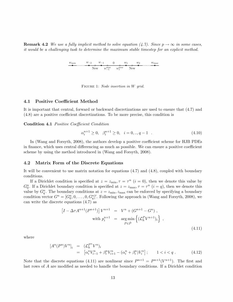
with large |wmin| and wmax. Note that our W grid does not contain the node w = 0, because ifw = 0 is in the grid, no information can be passed between the negative value nodes and positivevalue nodes. We set |w−1| and w1 to be small values close to zero. As Figure 1 shows, when theW grid is refined, a new node is inserted in between each two consecutive nodes, except for the pairw−1 and w1. Since w = 0 cannot be in the grid, we add two nodes of wnew

−1 = w−1

2 and wnew1 = w1

2into the grid.

Note that we could avoid this problem (near w = 0) by defining the control to be (pw) insteadof p. However, in the more realistic case of bounded p, it is more natural to impose constraints onp, rather than on (pw), hence we prefer to formulate the control (and constraints) in terms of thevariable p.

12

Remark 4.2 We use a fully implicit method to solve equation (4.7). Since p →∞ in some cases,it would be a challenging task to determine the maximum stable timestep for an explicit method.

ss s ss scc c cwnew−1New wnew

1 New

w−1w−2 w1 w2 wmaxwmin 0

Figure 1: Node insertion in W grid.

4.1 Positive Coefficient Method

It is important that central, forward or backward discretizations are used to ensure that (4.7) and(4.8) are a positive coefficient discretizations. To be more precise, this condition is

Condition 4.1 Positive Coefficient Condition

αn+1i ≥ 0, βn+1

i ≥ 0, i = 0, .., q − 1 . (4.10)

In (Wang and Forsyth, 2008), the authors develop a positive coefficient scheme for HJB PDEsin finance, which uses central differencing as much as possible. We can ensure a positive coefficientscheme by using the method introduced in (Wang and Forsyth, 2008).

4.2 Matrix Form of the Discrete Equations

It will be convenient to use matrix notation for equations (4.7) and (4.8), coupled with boundaryconditions.

If a Dirichlet condition is specified at z = zmin, τ = τn (i = 0), then we denote this value byGn

0 . If a Dirichlet boundary condition is specified at z = zmax, τ = τn (i = q), then we denote thisvalue by Gn

q . The boundary conditions at z = zmin, zmax can be enforced by specifying a boundarycondition vector Gn = [Gn

0 , 0, . . . , 0, Gnq ]′. Following the approach in (Wang and Forsyth, 2008), we

can write the discrete equations (4.7) as[I −∆τAn+1(Pn+1)

]V n+1 = V n + (Gn+1 −Gn) ,

with pn+1i = arg min

P∈P

{(LP

h V n+1)i

},

(4.11)

where

[An(Pn)V n]i = (LP n

h V n)i

=[αn

i V ni−1 + βn

i V ni+1 − (αn

i + βni )V n

i

]; 1 < i < q . (4.12)

Note that the discrete equations (4.11) are nonlinear since Pn+1 = Pn+1(V n+1). The first andlast rows of A are modified as needed to handle the boundary conditions. If a Dirichlet condition

13

is specified at i = 0, we set Gn0 to the appropriate value, and set the first row in An to be zero.

With a slight abuse of notation, we denote this last row in this case as (An)0 ≡ 0. Conversely, ifno boundary condition is required at i = 0, then we use forward differencing at node i = 0 (whichmeans that α0 = 0), and set Gn

0 = 0. The boundary condition at z = zmax, i = q, is handled in asimilar fashion.

The discrete equations (4.8) can be written as[I −∆τAn+1(Pn+1)

]Un+1 = Un + (Hn+1 −Hn) , (4.13)

where Pn+1 is given from the discrete equations (4.11), and H encodes the boundary conditions.

4.3 Convergence to the Viscosity Solution

PDE (4.5) is linear, since the optimal control is pre-computed. We can then obtain a classicalsolution of the linear PDE (4.5). However, PDE (4.4) is highly nonlinear, so the classical solutionmay not exist in general. In this case, we are seeking the viscosity solution (Barles, 1997; Crandallet al., 1992).

In (Pooley et al., 2003), examples were given in which seemingly reasonable discretizations ofnonlinear option pricing PDEs were unstable or converged to the incorrect solution. It is importantto ensure that we can generate discretizations which are guaranteed to converge to the viscositysolution (Barles, 1997; Crandall et al., 1992). Assuming that equation (4.4) satisfies the strongcomparison property (Barles and Burdeau, 1995; Barles, 1997; Chaumont, 2004), then, from (Barlesand Souganidis, 1991; Barles, 1997), a numerical scheme converges to the unique viscosity solutionif the method is pointwise consistent, stable (in the l∞ norm) and monotone.

It is straightforward, using the methods in (Barles and Jakobsen, 2005; Forsyth and Labahn,2008) to show that scheme (4.7) is monotone, pointwise consistent, and stable.

Assumption 4.1 (Strong Comparison) We assume that equation (4.4) satisfies the strong com-parison property.

Remark 4.3 If the control p is bounded, then from the results in (Chaumont, 2004; Barles andRouy, 1998) we can deduce that Equation (4.4) satisfies the strong comparison property on thelocalized computational domain D. In the unbounded control case, we violate one of the assumptionsin (Barles and Rouy, 1998) used in the proof of the strong comparison property. However, ournumerical results indicate that (pw) is always bounded. Hence, in the unbounded control case, wecould reformulate the problem in terms of a control (pw), and solve the problem with assumedbounds on (pw), which would then satisfy the conditions in (Barles and Rouy, 1998). However, itis not obvious how to obtain a priori bounds for (pw). In practical cases, we are more interested inbounded controls, so in this case we have that strong comparison holds.

Theorem 4.1 (Convergence to the Viscosity Solution) Provided that the original HJB sat-isfies Assumption 4.1, the boundary conditions given in Section 2.2 (or 3) and discretization (4.11)satisfies the positive coefficient condition (4.10) then scheme (4.11) converges to the viscosity solu-tion of equation (4.4).

14

Proof . Using the methods in (Barles and Jakobsen, 2005; Forsyth and Labahn, 2008), this canbe shown to follow from results in (Barles and Souganidis, 1991; Barles, 1997). We give a briefoverview of the proof.

Monotonicity: From the positive coefficient condition (equation (4.10)) and following the samemethod as in (Forsyth and Labahn, 2008), we can show that scheme (4.11) is monotone.

Pointwise consistency: From Appendix A, a simple Taylor series verifies consistency. Note thatsince we have either simple Dirichlet conditions, or the PDE at the boundary is the limit fromthe interior, then we need only use the classical definition of consistency here, not the morecomplex version discussed in (Barles and Souganidis, 1991; Barles, 1997; Chen and Forsyth,2008).

Stability: Using the same technique as in (Forsyth and Labahn, 2008), we can show that scheme(4.11) is l∞ stable by a maximum analysis. Again, this is a direct consequence of the positivecoefficient condition (4.10).

Under Assumption 4.1, there exists a unique, continuous viscosity solution to equation (4.4). Conse-quently, as shown in (Barles and Souganidis, 1991), if a discretization scheme is monotone, pointwiseconsistent and l∞ stable, then that scheme converges to the unique, continuous viscosity solution.

�

4.4 Policy Iteration

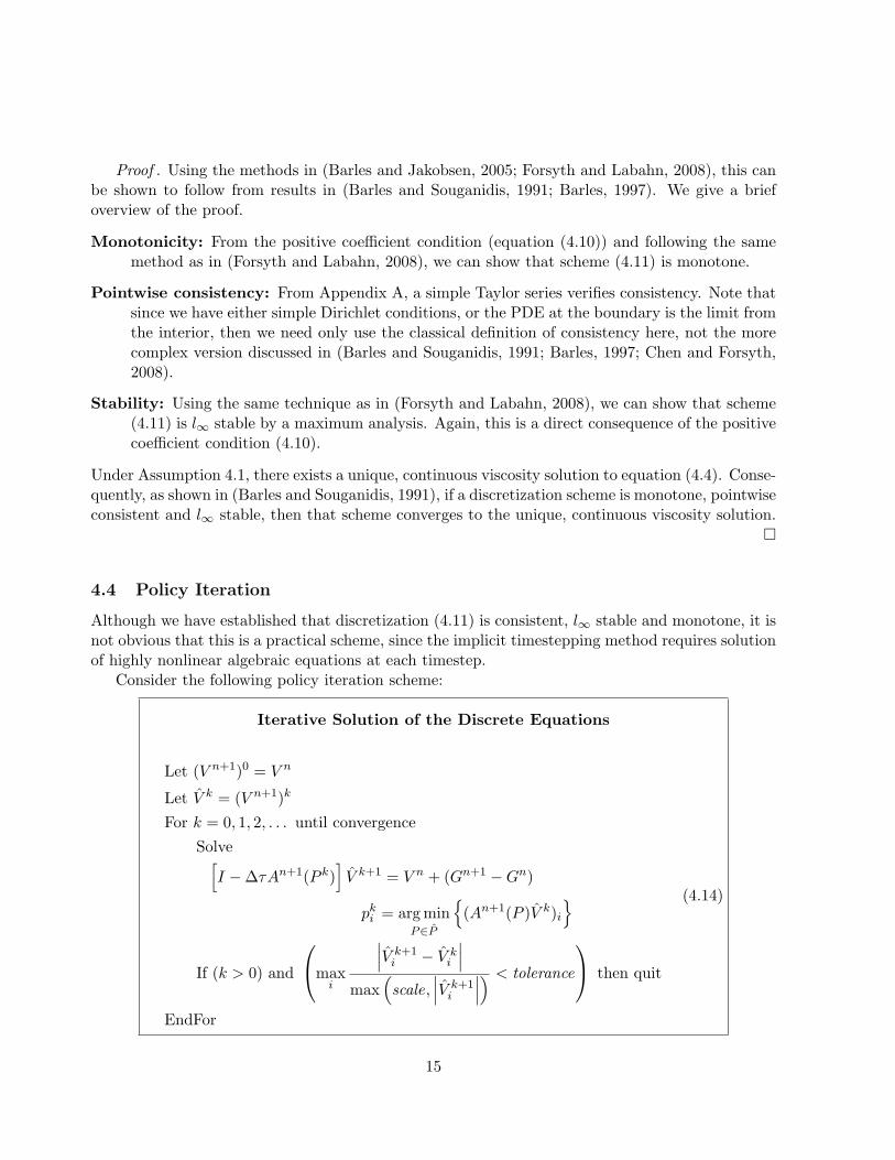
Although we have established that discretization (4.11) is consistent, l∞ stable and monotone, it isnot obvious that this is a practical scheme, since the implicit timestepping method requires solutionof highly nonlinear algebraic equations at each timestep.

Consider the following policy iteration scheme:

Iterative Solution of the Discrete Equations

Let (V n+1)0 = V n

Let V k = (V n+1)k

For k = 0, 1, 2, . . . until convergenceSolve[

I −∆τAn+1(P k)]V k+1 = V n + (Gn+1 −Gn)

pki = arg min

P∈P

{(An+1(P )V k)i

}

If (k > 0) and

maxi

∣∣∣V k+1i − V k

i

∣∣∣max

(scale,

∣∣∣V k+1i

∣∣∣) < tolerance

then quit

EndFor

(4.14)

15

The term scale in scheme (4.14) is used to ensure that unrealistic levels of accuracy are notrequired when the value is very small. Typically, we use scale = 1 in this paper, and tolerance =10−6.

Theorem 4.2 (Convergence of Iteration (4.14)) If the discretization (4.11) satisfies the pos-itive coefficient condition (4.10), then the policy iteration (4.14) converges to the unique solutionof equation (4.11) for any initial iterate V 0. Moreover, the iterates converge monotonically.

Proof . The proof is given in (Wang and Forsyth, 2008). �

Remark 4.4 An important step in iteration (4.14) is to determine the optimal control pki for

each node i at each iteration. For the problems we study in this paper, the objective function(LP n+1

h V n+1)i is a piecewise quadratic function of the control. The optimal control at each nodecan then be easily determined.

In the case where the objective function is a complicated function of the control, it may be difficultto determine the optimal control analytically. If the control set P is bounded, then we can replacethe set of admissible controls P by an approximation P. In this case, we define P = [q0, q1, ..., qm],where q0 = pmin, qm = pmax, and

maxi

(qi+1 − qi) = h . (4.15)

As long as h → 0 as the mesh and timesteps tend to zero, then replacing P by P is a consistentapproximation (Wang and Forsyth, 2008), and hence converges to the viscosity solution.

Remark 4.5 We follow the approach given in (Wang and Forsyth, 2008), which uses central dif-ferencing as much as possible, to ensure a positive coefficient scheme with a maximal use of a secondorder method in the W (or X) direction. When we use central differencing as much as possible, thelocal objective function at each node is a discontinuous function of the control. However, (Wangand Forsyth, 2008) shows that the proof of convergence of the iterative scheme for solution of thefully implicit discretized algebraic equations does not require continuity of the local objective func-tion. Hence convergence of the iterative algorithm for solving the nonlinear discretized equations isguaranteed.

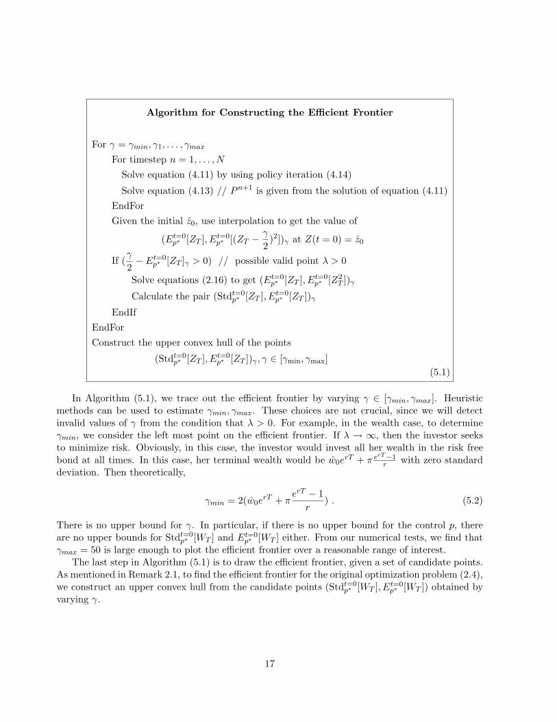
5 Algorithm for Construction of the Efficient Frontier

Given an initial value z0, Algorithm (5.1) is used to obtain the efficient frontier. Since the Z grid isdiscretized over the interval [zmin, zmax], we can use Algorithm (5.1) to obtain the efficient frontierfor any initial wealth z0 ∈ [zmin, zmax] by interpolation. Of course, if we choose z0 to be a node inthe discretized Z grid, then there is no interpolation error.

16

Algorithm for Constructing the Efficient Frontier

For γ = γmin, γ1, . . . , γmax

For timestep n = 1, . . . , N

Solve equation (4.11) by using policy iteration (4.14)

Solve equation (4.13) // Pn+1 is given from the solution of equation (4.11)EndForGiven the initial z0, use interpolation to get the value of

(Et=0p∗ [ZT ], Et=0

p∗ [(ZT −γ

2)2])γ at Z(t = 0) = z0

If (γ

2− Et=0

p∗ [ZT ]γ > 0) // possible valid point λ > 0

Solve equations (2.16) to get (Et=0p∗ [ZT ], Et=0

p∗ [Z2T ])γ

Calculate the pair (Stdt=0p∗ [ZT ], Et=0

p∗ [ZT ])γ

EndIfEndForConstruct the upper convex hull of the points

(Stdt=0p∗ [ZT ], Et=0

p∗ [ZT ])γ , γ ∈ [γmin, γmax](5.1)

In Algorithm (5.1), we trace out the efficient frontier by varying γ ∈ [γmin, γmax]. Heuristicmethods can be used to estimate γmin, γmax. These choices are not crucial, since we will detectinvalid values of γ from the condition that λ > 0. For example, in the wealth case, to determineγmin, we consider the left most point on the efficient frontier. If λ → ∞, then the investor seeksto minimize risk. Obviously, in this case, the investor would invest all her wealth in the risk freebond at all times. In this case, her terminal wealth would be w0e

rT + π erT−1r with zero standard

deviation. Then theoretically,

γmin = 2(w0erT + π

erT − 1r

) . (5.2)

There is no upper bound for γ. In particular, if there is no upper bound for the control p, thereare no upper bounds for Stdt=0

p∗ [WT ] and Et=0p∗ [WT ] either. From our numerical tests, we find that

γmax = 50 is large enough to plot the efficient frontier over a reasonable range of interest.The last step in Algorithm (5.1) is to draw the efficient frontier, given a set of candidate points.

As mentioned in Remark 2.1, to find the efficient frontier for the original optimization problem (2.4),we construct an upper convex hull from the candidate points (Stdt=0

p∗ [WT ], Et=0p∗ [WT ]) obtained by

varying γ.

17

6 Numerical Results

In this section, we carry out numerical tests for the defined contribution pension plan problem.We examine both the wealth case (addressed in Section 2) and the wealth-to-income ratio case(addressed in Section 3).

6.1 Wealth Case

6.1.1 Allowing Bankruptcy

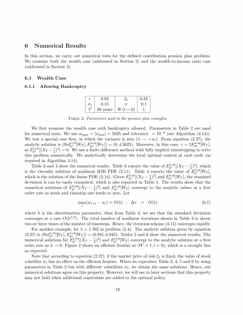
r 0.03 ξ1 0.33σ1 0.15 π 0.1T 20 years W (t = 0) 1

Table 2: Parameters used in the pension plan examples.

We first examine the wealth case with bankruptcy allowed. Parameters in Table 2 are usedfor numerical tests. We use wmax = |wmin| = 5925 and tolerance = 10−6 (see Algorithm (4.14)).We test a special case first, in which the variance is zero (λ → +∞). From equation (2.27), theanalytic solution is (Stdt=0

p∗ [WT ], Et=0p∗ [WT ]) = (0, 4.5625). Moreover, in this case, γ = 2Et=0

p∗ [WT ],so Et=0

p∗ [(XT − γ2 )2] = 0. We use a finite difference method with fully implicit timestepping to solve

this problem numerically. We analytically determine the local optimal control at each node (asrequired in Algorithm 4.14).

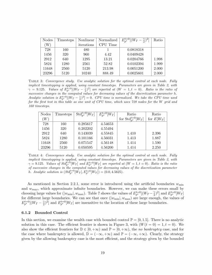
Table 3 and 4 show the numerical results. Table 3 reports the value of Et=0p∗ [(XT − γ

2 )2], whichis the viscosity solution of nonlinear HJB PDE (2.11). Table 4 reports the value of Et=0

p∗ [WT ],which is the solution of the linear PDE (2.14). Given Et=0

p∗ [(XT − γ2 )2] and Et=0

p∗ [WT ], the standarddeviation is can be easily computed, which is also reported in Table 4. The results show that thenumerical solutions of Et=0

p∗ [(XT − γ2 )2] and Et=0

p∗ [WT ] converge to the analytic values at a firstorder rate as mesh and timestep size tends to zero. Let

maxi

(wi+1 − wi) = O(h) ; ∆τ = O(h) (6.1)

where h is the discretization parameter, then from Table 4, we see that the standard deviationconverges at a rate O(h1/2). The total number of nonlinear iterations shown in Table 3 is abouttwo or three times of the number of timesteps. Hence, the iteration scheme (4.14) converges rapidly.

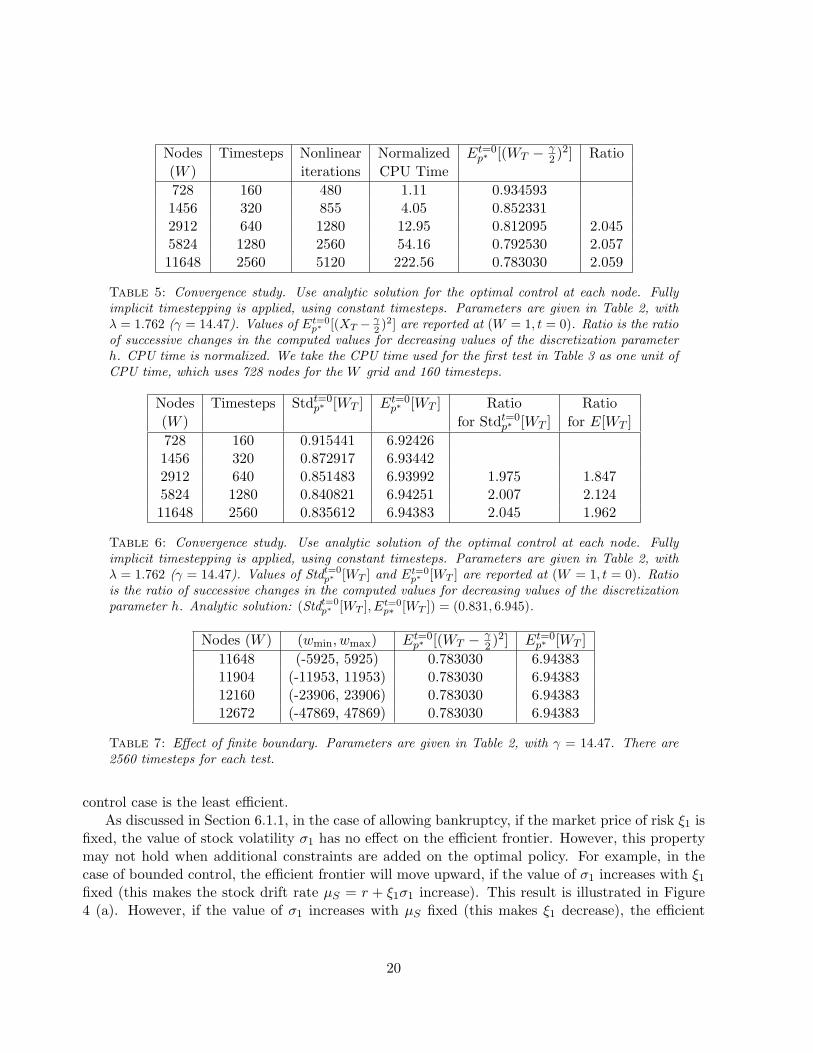
For another example, let λ = 1.762 in problem (2.4). The analytic solution given by equation(2.27) is (Stdt=0

p∗ [WT ], Et=0p∗ [WT ]) = (0.831, 6.945). Tables 5 and 6 show the numerical results. The

numerical solutions for Et=0p∗ [(XT − γ

2 )2] and Et=0p∗ [WT ] converge to the analytic solution at a first

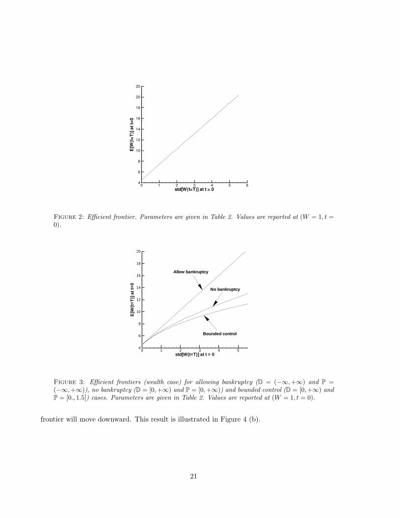
order rate as h → 0. Figure 2 shows an efficient frontier at (W = 1, t = 0), which is a straight lineas expected.

Note that according to equation (2.27), if the market price of risk ξ1 is fixed, the value of stockvolatility σ1 has no effect on the efficient frontier. When we reproduce Table 3, 4, 5 and 6 by usingparameters in Table 2 but with different volatilities σ1, we obtain the same solutions. Hence, ournumerical solutions agree on this property. However, we will see in later sections that this propertymay not hold when additional constraints are added to the optimal policy.

18

Nodes Timesteps Nonlinear Normalized Et=0p∗ [(WT − γ

2 )2] Ratio(W) iterations CPU Time728 160 480 1 0.08183181456 320 960 4.42 0.04094282912 640 1295 13.21 0.0204766 1.9985824 1280 2561 52.82 0.0102394 1.99911648 2560 5120 213.98 0.0051200 2.00023296 5120 10240 888.49 0.0025601 2.000

Table 3: Convergence study. Use analytic solution for the optimal control at each node. Fullyimplicit timestepping is applied, using constant timesteps. Parameters are given in Table 2, withγ = 9.125. Values of Et=0

p∗ [(WT − γ2 )2] are reported at (W = 1, t = 0). Ratio is the ratio of

successive changes in the computed values for decreasing values of the discretization parameter h.Analytic solution is Et=0

p∗ [(WT − γ2 )2] = 0. CPU time is normalized. We take the CPU time used

for the first test in this table as one unit of CPU time, which uses 728 nodes for the W grid and160 timesteps.

Nodes Timesteps Stdt=0p∗ [WT ] Et=0

p∗ [WT ] Ratio Ratio(W ) for Stdt=0

p∗ [WT ] for E[WT ]728 160 0.285617 4.546531456 320 0.202202 4.554942912 640 0.143039 4.55845 1.410 2.3965824 1280 0.101166 4.56031 1.413 1.88711648 2560 0.071547 4.56148 1.414 1.59023296 5120 0.050595 4.56200 1.414 2.250

Table 4: Convergence study. Use analytic solution for the optimal control at each node. Fullyimplicit timestepping is applied, using constant timesteps. Parameters are given in Table 2, withγ = 9.125. Values of Stdt=0

p∗ [WT ] and Et=0p∗ [WT ] are reported at (W = 1, t = 0). Ratio is the ratio

of successive changes in the computed values for decreasing values of the discretization parameterh. Analytic solution is (Stdt=0

p∗ [WT ], Et=0p∗ [WT ]) = (0.0, 4.5625).

As mentioned in Section 2.2.1, some error is introduced using the artificial boundaries wmin

and wmax, which approximate infinite boundaries. However, we can make these errors small bychoosing large values for (|wmin|, wmax). Table 7 shows the values of Et=0

p∗ [(WT − γ2 )2] and Et=0

p∗ [WT ]for different large boundaries. We can see that once (|wmin|, wmax) are large enough, the values ofEt=0

p∗ [(WT − γ2 )2] and Et=0

p∗ [WT ] are insensitive to the location of these large boundaries.

6.1.2 Bounded Control

In this section, we examine the wealth case with bounded control P = [0, 1.5]. There is no analyticsolution in this case. The efficient frontier is shown in Figure 3, with (W (t = 0) = 1, t = 0). Wealso show the efficient frontiers for D ∈ [0,+∞) and P = [0,+∞), the no bankruptcy case, and forthe case where bankruptcy is allowed, D = (−∞,+∞) and P = (−∞,+∞). Clearly, the strategygiven by the allowing bankruptcy case is the most efficient, and the strategy given by the bounded

19

Nodes Timesteps Nonlinear Normalized Et=0p∗ [(WT − γ

2 )2] Ratio(W ) iterations CPU Time728 160 480 1.11 0.9345931456 320 855 4.05 0.8523312912 640 1280 12.95 0.812095 2.0455824 1280 2560 54.16 0.792530 2.05711648 2560 5120 222.56 0.783030 2.059

Table 5: Convergence study. Use analytic solution for the optimal control at each node. Fullyimplicit timestepping is applied, using constant timesteps. Parameters are given in Table 2, withλ = 1.762 (γ = 14.47). Values of Et=0

p∗ [(XT − γ2 )2] are reported at (W = 1, t = 0). Ratio is the ratio

of successive changes in the computed values for decreasing values of the discretization parameterh. CPU time is normalized. We take the CPU time used for the first test in Table 3 as one unit ofCPU time, which uses 728 nodes for the W grid and 160 timesteps.

Nodes Timesteps Stdt=0p∗ [WT ] Et=0

p∗ [WT ] Ratio Ratio(W ) for Stdt=0

p∗ [WT ] for E[WT ]728 160 0.915441 6.924261456 320 0.872917 6.934422912 640 0.851483 6.93992 1.975 1.8475824 1280 0.840821 6.94251 2.007 2.12411648 2560 0.835612 6.94383 2.045 1.962

Table 6: Convergence study. Use analytic solution of the optimal control at each node. Fullyimplicit timestepping is applied, using constant timesteps. Parameters are given in Table 2, withλ = 1.762 (γ = 14.47). Values of Stdt=0

p∗ [WT ] and Et=0p∗ [WT ] are reported at (W = 1, t = 0). Ratio

is the ratio of successive changes in the computed values for decreasing values of the discretizationparameter h. Analytic solution: (Stdt=0

p∗ [WT ], Et=0p∗ [WT ]) = (0.831, 6.945).

Nodes (W ) (wmin, wmax) Et=0p∗ [(WT − γ

2 )2] Et=0p∗ [WT ]

11648 (-5925, 5925) 0.783030 6.9438311904 (-11953, 11953) 0.783030 6.9438312160 (-23906, 23906) 0.783030 6.9438312672 (-47869, 47869) 0.783030 6.94383

Table 7: Effect of finite boundary. Parameters are given in Table 2, with γ = 14.47. There are2560 timesteps for each test.

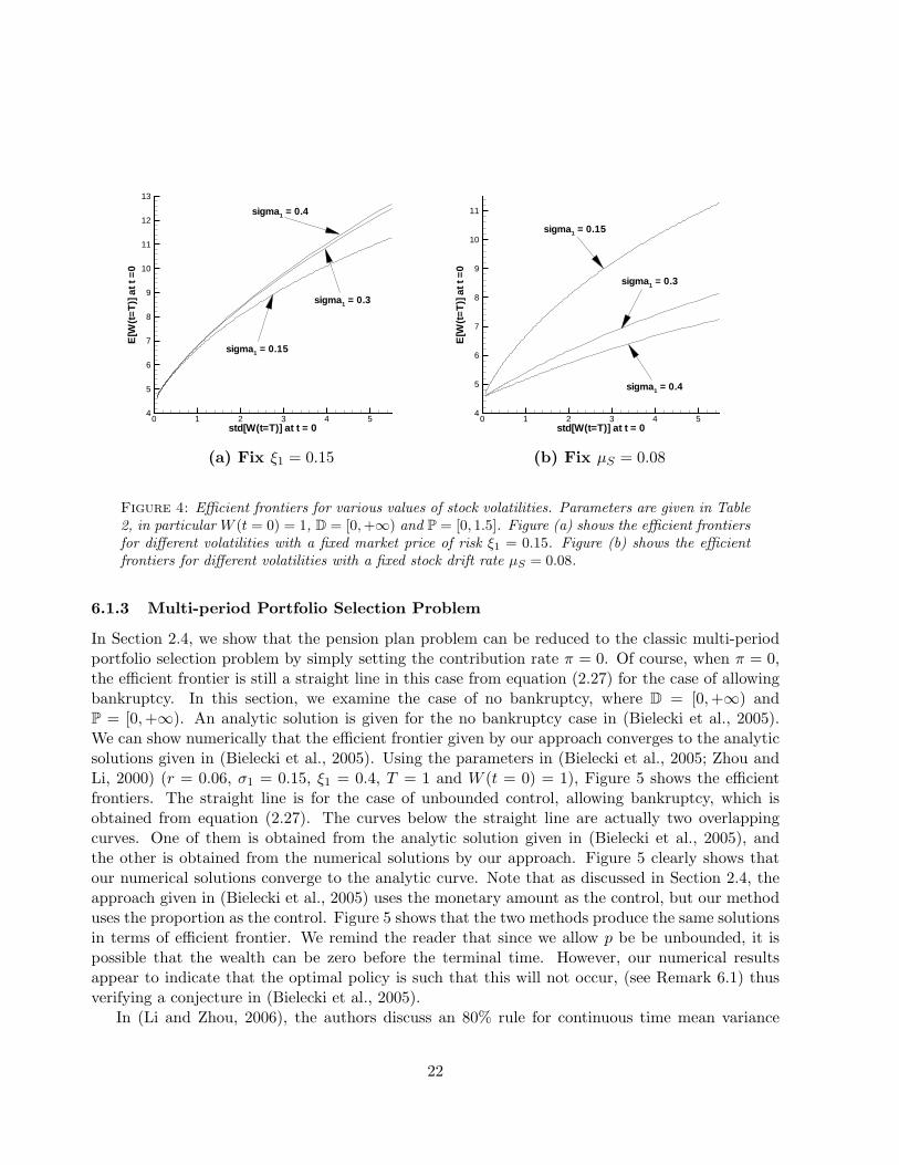
control case is the least efficient.As discussed in Section 6.1.1, in the case of allowing bankruptcy, if the market price of risk ξ1 is

fixed, the value of stock volatility σ1 has no effect on the efficient frontier. However, this propertymay not hold when additional constraints are added on the optimal policy. For example, in thecase of bounded control, the efficient frontier will move upward, if the value of σ1 increases with ξ1

fixed (this makes the stock drift rate µS = r + ξ1σ1 increase). This result is illustrated in Figure4 (a). However, if the value of σ1 increases with µS fixed (this makes ξ1 decrease), the efficient

20

std[W(t=T)] at t = 0

E[W

(t=T)

]att

=0

0 1 2 3 4 5 64

6

8

10

12

14

16

18

20

22

Figure 2: Efficient frontier. Parameters are given in Table 2. Values are reported at (W = 1, t =0).

std[W(t=T)] at t = 0

E[W

(t=

T)]

att=

0

0 1 2 3 4 54

6

8

10

12

14

16

18

20

Allow bankruptcy

No bankruptcy

Bounded control

Figure 3: Efficient frontiers (wealth case) for allowing bankruptcy (D = (−∞,+∞) and P =(−∞,+∞)), no bankruptcy (D = [0,+∞) and P = [0,+∞)) and bounded control (D = [0,+∞) andP = [0., 1.5]) cases. Parameters are given in Table 2. Values are reported at (W = 1, t = 0).

frontier will move downward. This result is illustrated in Figure 4 (b).

21

std[W(t=T)] at t = 0

E[W

(t=

T)]

att=

0

0 1 2 3 4 54

5

6

7

8

9

10

11

12

13

sigma1 = 0.3

sigma1 = 0.15

sigma1 = 0.4

std[W(t=T)] at t = 0

E[W

(t=

T)]

att=

0

0 1 2 3 4 54

5

6

7

8

9

10

11

sigma1 = 0.3

sigma1 = 0.15

sigma1 = 0.4

(a) Fix ξ1 = 0.15 (b) Fix µS = 0.08

Figure 4: Efficient frontiers for various values of stock volatilities. Parameters are given in Table2, in particular W (t = 0) = 1, D = [0,+∞) and P = [0, 1.5]. Figure (a) shows the efficient frontiersfor different volatilities with a fixed market price of risk ξ1 = 0.15. Figure (b) shows the efficientfrontiers for different volatilities with a fixed stock drift rate µS = 0.08.

6.1.3 Multi-period Portfolio Selection Problem

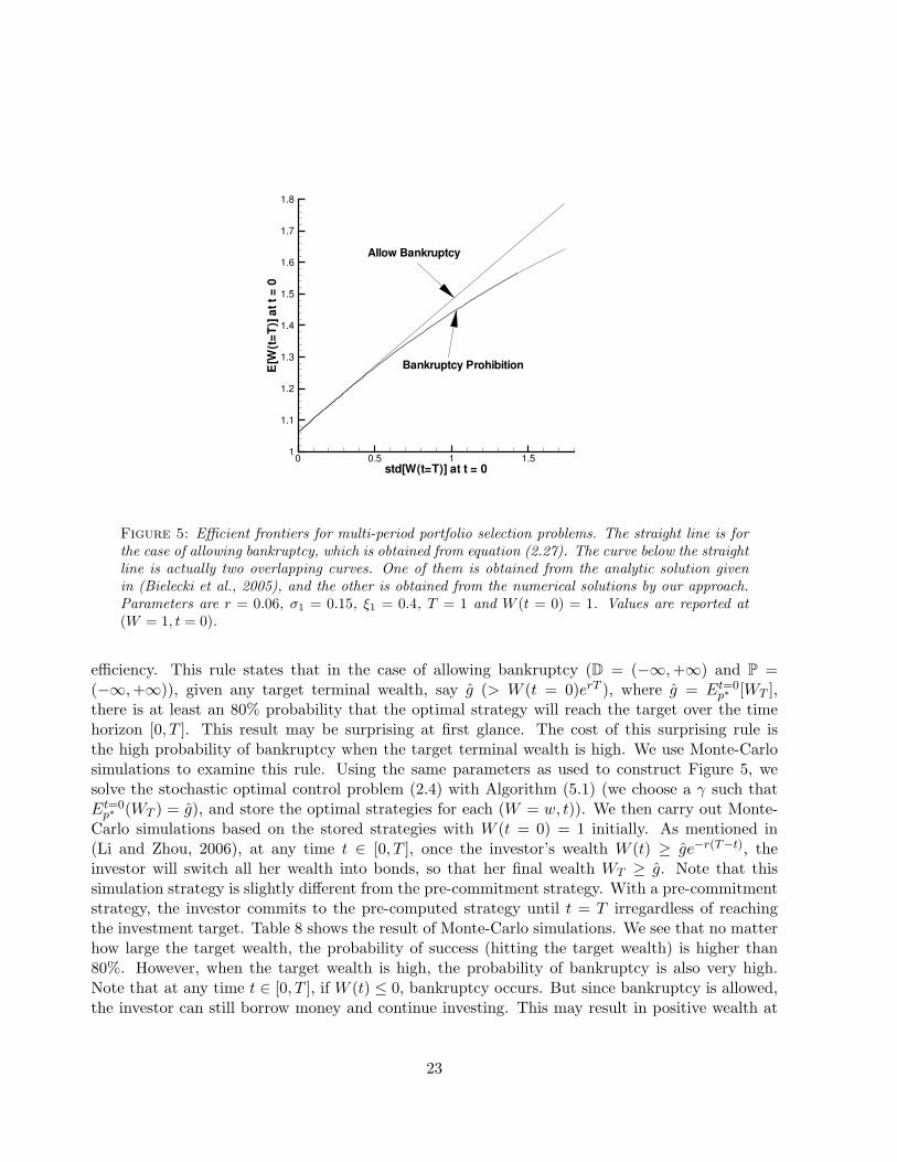
In Section 2.4, we show that the pension plan problem can be reduced to the classic multi-periodportfolio selection problem by simply setting the contribution rate π = 0. Of course, when π = 0,the efficient frontier is still a straight line in this case from equation (2.27) for the case of allowingbankruptcy. In this section, we examine the case of no bankruptcy, where D = [0,+∞) andP = [0,+∞). An analytic solution is given for the no bankruptcy case in (Bielecki et al., 2005).We can show numerically that the efficient frontier given by our approach converges to the analyticsolutions given in (Bielecki et al., 2005). Using the parameters in (Bielecki et al., 2005; Zhou andLi, 2000) (r = 0.06, σ1 = 0.15, ξ1 = 0.4, T = 1 and W (t = 0) = 1), Figure 5 shows the efficientfrontiers. The straight line is for the case of unbounded control, allowing bankruptcy, which isobtained from equation (2.27). The curves below the straight line are actually two overlappingcurves. One of them is obtained from the analytic solution given in (Bielecki et al., 2005), andthe other is obtained from the numerical solutions by our approach. Figure 5 clearly shows thatour numerical solutions converge to the analytic curve. Note that as discussed in Section 2.4, theapproach given in (Bielecki et al., 2005) uses the monetary amount as the control, but our methoduses the proportion as the control. Figure 5 shows that the two methods produce the same solutionsin terms of efficient frontier. We remind the reader that since we allow p be be unbounded, it ispossible that the wealth can be zero before the terminal time. However, our numerical resultsappear to indicate that the optimal policy is such that this will not occur, (see Remark 6.1) thusverifying a conjecture in (Bielecki et al., 2005).

In (Li and Zhou, 2006), the authors discuss an 80% rule for continuous time mean variance

22

std[W(t=T)] at t = 0

E[W

(t=T)

]att

=0

0 0.5 1 1.51

1.1

1.2

1.3

1.4

1.5

1.6

1.7

1.8

Allow Bankruptcy

Bankruptcy Prohibition

Figure 5: Efficient frontiers for multi-period portfolio selection problems. The straight line is forthe case of allowing bankruptcy, which is obtained from equation (2.27). The curve below the straightline is actually two overlapping curves. One of them is obtained from the analytic solution givenin (Bielecki et al., 2005), and the other is obtained from the numerical solutions by our approach.Parameters are r = 0.06, σ1 = 0.15, ξ1 = 0.4, T = 1 and W (t = 0) = 1. Values are reported at(W = 1, t = 0).

efficiency. This rule states that in the case of allowing bankruptcy (D = (−∞,+∞) and P =(−∞,+∞)), given any target terminal wealth, say g (> W (t = 0)erT ), where g = Et=0

p∗ [WT ],there is at least an 80% probability that the optimal strategy will reach the target over the timehorizon [0, T ]. This result may be surprising at first glance. The cost of this surprising rule isthe high probability of bankruptcy when the target terminal wealth is high. We use Monte-Carlosimulations to examine this rule. Using the same parameters as used to construct Figure 5, wesolve the stochastic optimal control problem (2.4) with Algorithm (5.1) (we choose a γ such thatEt=0

p∗ (WT ) = g), and store the optimal strategies for each (W = w, t)). We then carry out Monte-Carlo simulations based on the stored strategies with W (t = 0) = 1 initially. As mentioned in(Li and Zhou, 2006), at any time t ∈ [0, T ], once the investor’s wealth W (t) ≥ ge−r(T−t), theinvestor will switch all her wealth into bonds, so that her final wealth WT ≥ g. Note that thissimulation strategy is slightly different from the pre-commitment strategy. With a pre-commitmentstrategy, the investor commits to the pre-computed strategy until t = T irregardless of reachingthe investment target. Table 8 shows the result of Monte-Carlo simulations. We see that no matterhow large the target wealth, the probability of success (hitting the target wealth) is higher than80%. However, when the target wealth is high, the probability of bankruptcy is also very high.Note that at any time t ∈ [0, T ], if W (t) ≤ 0, bankruptcy occurs. But since bankruptcy is allowed,the investor can still borrow money and continue investing. This may result in positive wealth at

23

some later time. The last column in Table 8 shows the probability of bankruptcy at time T , whichis much lower than the probability of bankruptcy at any time t ∈ [0, T ].

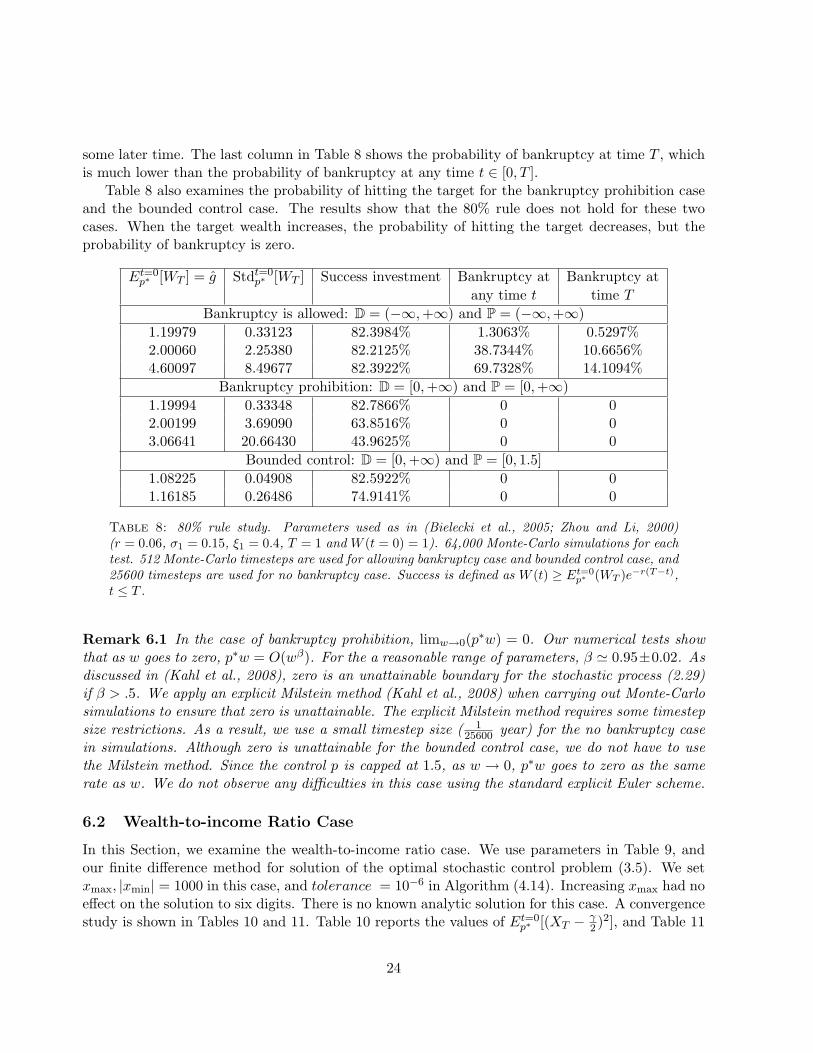
Table 8 also examines the probability of hitting the target for the bankruptcy prohibition caseand the bounded control case. The results show that the 80% rule does not hold for these twocases. When the target wealth increases, the probability of hitting the target decreases, but theprobability of bankruptcy is zero.

Et=0p∗ [WT ] = g Stdt=0

p∗ [WT ] Success investment Bankruptcy at Bankruptcy atany time t time T

Bankruptcy is allowed: D = (−∞,+∞) and P = (−∞,+∞)1.19979 0.33123 82.3984% 1.3063% 0.5297%2.00060 2.25380 82.2125% 38.7344% 10.6656%4.60097 8.49677 82.3922% 69.7328% 14.1094%

Bankruptcy prohibition: D = [0,+∞) and P = [0,+∞)1.19994 0.33348 82.7866% 0 02.00199 3.69090 63.8516% 0 03.06641 20.66430 43.9625% 0 0

Bounded control: D = [0,+∞) and P = [0, 1.5]1.08225 0.04908 82.5922% 0 01.16185 0.26486 74.9141% 0 0

Table 8: 80% rule study. Parameters used as in (Bielecki et al., 2005; Zhou and Li, 2000)(r = 0.06, σ1 = 0.15, ξ1 = 0.4, T = 1 and W (t = 0) = 1). 64,000 Monte-Carlo simulations for eachtest. 512 Monte-Carlo timesteps are used for allowing bankruptcy case and bounded control case, and25600 timesteps are used for no bankruptcy case. Success is defined as W (t) ≥ Et=0

p∗ (WT )e−r(T−t),t ≤ T .

Remark 6.1 In the case of bankruptcy prohibition, limw→0(p∗w) = 0. Our numerical tests showthat as w goes to zero, p∗w = O(wβ). For the a reasonable range of parameters, β ' 0.95±0.02. Asdiscussed in (Kahl et al., 2008), zero is an unattainable boundary for the stochastic process (2.29)if β > .5. We apply an explicit Milstein method (Kahl et al., 2008) when carrying out Monte-Carlosimulations to ensure that zero is unattainable. The explicit Milstein method requires some timestepsize restrictions. As a result, we use a small timestep size ( 1

25600 year) for the no bankruptcy casein simulations. Although zero is unattainable for the bounded control case, we do not have to usethe Milstein method. Since the control p is capped at 1.5, as w → 0, p∗w goes to zero as the samerate as w. We do not observe any difficulties in this case using the standard explicit Euler scheme.

6.2 Wealth-to-income Ratio Case

In this Section, we examine the wealth-to-income ratio case. We use parameters in Table 9, andour finite difference method for solution of the optimal stochastic control problem (3.5). We setxmax, |xmin| = 1000 in this case, and tolerance = 10−6 in Algorithm (4.14). Increasing xmax had noeffect on the solution to six digits. There is no known analytic solution for this case. A convergencestudy is shown in Tables 10 and 11. Table 10 reports the values of Et=0

p∗ [(XT − γ2 )2], and Table 11

24

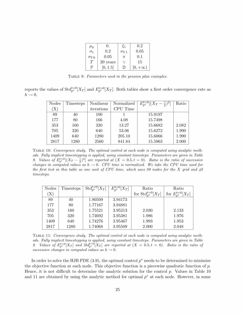
µy 0. ξ1 0.2σ1 0.2 σY 1 0.05σY 0 0.05 π 0.1T 20 years γ 15P [0, 1.5] D [0,+∞)

Table 9: Parameters used in the pension plan examples.

reports the values of Stdt=0p∗ [XT ] and Et=0

p∗ [XT ]. Both tables show a first order convergence rate ash → 0.

Nodes Timesteps Nonlinear Normalized Et=0p∗ [(XT − γ

2 )2] Ratio(X) iterations CPU Time89 40 100 1 15.9197177 80 166 4.08 15.7498353 160 320 13.27 15.6682 2.082705 320 640 53.06 15.6272 1.9901409 640 1280 205.10 15.6066 1.9902817 1280 2560 841.84 15.5963 2.000

Table 10: Convergence study. The optimal control at each node is computed using analytic meth-ods. Fully implicit timestepping is applied, using constant timesteps. Parameters are given in Table9. Values of Et=0

p∗ [(XT − γ2 )2] are reported at (X = 0.5, t = 0). Ratio is the ratio of successive

changes in computed values as h → 0. CPU time is normalized. We take the CPU time used forthe first test in this table as one unit of CPU time, which uses 89 nodes for the X grid and 40timesteps.

Nodes Timesteps Stdt=0p∗ [XT ] Et=0

p∗ [XT ] Ratio Ratio(X) for Stdt=0

p∗ [XT ] for Et=0p∗ [XT ]

89 40 1.80509 3.94173177 80 1.77167 3.94881353 160 1.75521 3.95213 2.030 2.133705 320 1.74692 3.95381 1.986 1.9761409 640 1.74276 3.95467 1.993 1.9532817 1280 1.74068 3.95509 2.000 2.048

Table 11: Convergence study. The optimal control at each node is computed using analytic meth-ods. Fully implicit timestepping is applied, using constant timesteps. Parameters are given in Table9. Values of Et=0

p∗ [XT ] and Stdt=0p∗ [XT ] are reported at (X = 0.5, t = 0). Ratio is the ratio of

successive changes in computed values as h → 0.

In order to solve the HJB PDE (3.9), the optimal control p∗ needs to be determined to minimizethe objective function at each node. This objective function is a piecewise quadratic function of p.Hence, it is not difficult to determine the analytic solution for the control p. Values in Table 10and 11 are obtained by using the analytic method for optimal p∗ at each node. However, in some

25

cases, it is not easy to determine the analytic solution for the control. In such cases, the controlset P can be discretized to a set P (as discussed in Remark 4.4), and the optimal control can bedetermined by linear search. The convergence to viscosity solution of this method is proven in(Wang and Forsyth, 2008). Table 12 and 13 show a convergence study with the discretized control.Again, a first order convergence rate is obtained in both tables. Of course, this method requiresmuch more CPU time compared to the method used by Table 10 and 11. This is simply due to thecomparatively crude method used to find the optimal control at each grid node.

Nodes Timesteps Nonlinear Normalized Et=0p∗ [(XT − γ

2 )2] Ratio(X × P) iterations CPU Time89 × 21 40 101 4.08 15.9242177 × 41 80 166 22.45 15.7509353 × 81 160 320 161.22 15.6684 2.101705 × 161 320 640 1276.53 15.6272 2.0021409 × 321 640 1280 9917.35 15.6066 2.0002817 × 641 1280 2560 76102.04 15.5963 2.000

Table 12: Convergence study. Use discretized control set P and linear search to find the optimalcontrol. Fully implicit timestepping is applied, using constant timesteps. Parameters are given inTable 9. Values of Et=0

p∗ [(XT − γ2 )2] are reported at (X = 0.5, t = 0). Ratio is the ratio of successive

changes in computed values as h → 0. CPU time is normalized. We take the CPU time used for thefirst test in Table 10 as one unit of CPU time, which uses 89 nodes for X grid and 40 timesteps.

Nodes Timesteps Stdt=0p∗ [XT ] Et=0

p∗ [XT ] Ratio Ratio(X × P) for Stdt=0

p∗ [XT ] for Et=0p∗ [XT ]

89 × 21 40 1.80701 3.94206177 × 41 80 1.77144 3.94854353 × 81 160 1.75529 3.95213 2.202 1.805705 × 161 320 1.74693 3.95381 1.932 2.1371409 × 321 640 1.74276 3.95466 2.005 1.9762817 × 641 1280 1.74068 3.95509 2.005 1.977

Table 13: Convergence study. Use discretized control set P and linear search to find the optimalcontrol. Fully implicit timestepping is applied, using constant timesteps. Parameters are given inTable 9. Values of Et=0

p∗ [XT ] and Stdt=0p∗ [XT ] are reported at (X = 0.5, t = 0). Ratio is the ratio of

successive changes in computed values as h → 0.

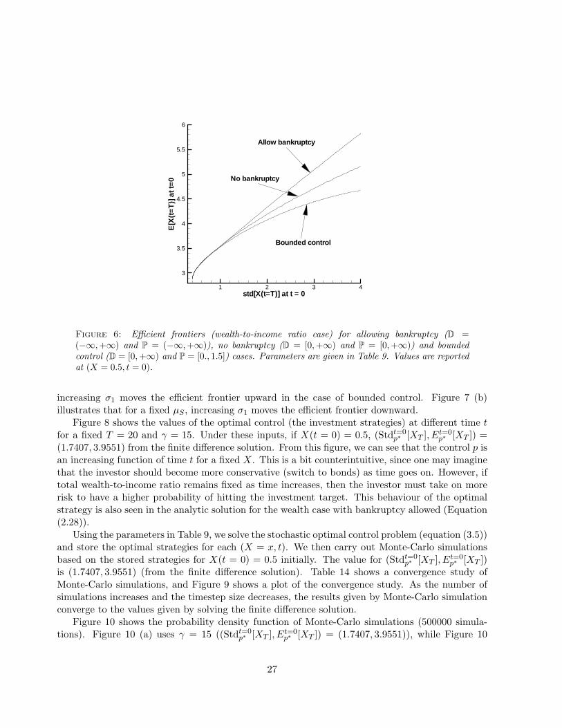
Figure 6 shows the efficient frontiers allowing bankruptcy, no bankruptcy and bounded controlcases. Again, the strategy given by the allowing bankruptcy case is the most efficient, and thestrategy given by the bounded control case is the least efficient.

In Section 6.1, we have discussed the effects of changing the value of σ1 on the efficient frontiersolution. We obtain similar results for the wealth-to-income case. For a fixed ξ1, different valuesof σ1 give the same efficient frontier solution in the case of allowing bankruptcy. However, thisproperty does not hold for the bounded control case. Figure 7 (a) illustrates that for a fixed ξ1,

26

std[X(t=T)] at t = 0

E[X

(t=

T)]

att=

0

1 2 3 4

3

3.5

4

4.5

5

5.5

6

Allow bankruptcy

No bankruptcy

Bounded control

Figure 6: Efficient frontiers (wealth-to-income ratio case) for allowing bankruptcy (D =(−∞,+∞) and P = (−∞,+∞)), no bankruptcy (D = [0,+∞) and P = [0,+∞)) and boundedcontrol (D = [0,+∞) and P = [0., 1.5]) cases. Parameters are given in Table 9. Values are reportedat (X = 0.5, t = 0).

increasing σ1 moves the efficient frontier upward in the case of bounded control. Figure 7 (b)illustrates that for a fixed µS , increasing σ1 moves the efficient frontier downward.

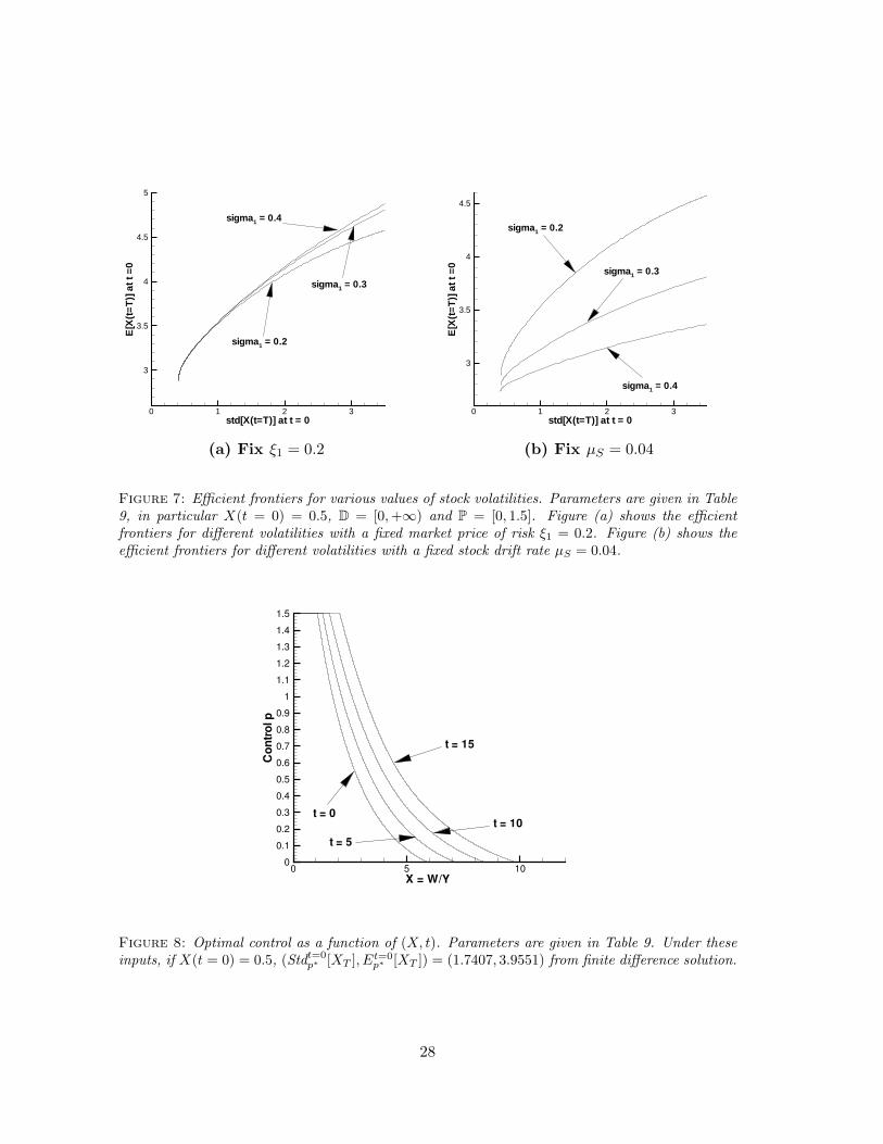
Figure 8 shows the values of the optimal control (the investment strategies) at different time tfor a fixed T = 20 and γ = 15. Under these inputs, if X(t = 0) = 0.5, (Stdt=0

p∗ [XT ], Et=0p∗ [XT ]) =

(1.7407, 3.9551) from the finite difference solution. From this figure, we can see that the control p isan increasing function of time t for a fixed X. This is a bit counterintuitive, since one may imaginethat the investor should become more conservative (switch to bonds) as time goes on. However, iftotal wealth-to-income ratio remains fixed as time increases, then the investor must take on morerisk to have a higher probability of hitting the investment target. This behaviour of the optimalstrategy is also seen in the analytic solution for the wealth case with bankruptcy allowed (Equation(2.28)).

Using the parameters in Table 9, we solve the stochastic optimal control problem (equation (3.5))and store the optimal strategies for each (X = x, t). We then carry out Monte-Carlo simulationsbased on the stored strategies for X(t = 0) = 0.5 initially. The value for (Stdt=0

p∗ [XT ], Et=0p∗ [XT ])

is (1.7407, 3.9551) (from the finite difference solution). Table 14 shows a convergence study ofMonte-Carlo simulations, and Figure 9 shows a plot of the convergence study. As the number ofsimulations increases and the timestep size decreases, the results given by Monte-Carlo simulationconverge to the values given by solving the finite difference solution.

Figure 10 shows the probability density function of Monte-Carlo simulations (500000 simula-tions). Figure 10 (a) uses γ = 15 ((Stdt=0

p∗ [XT ], Et=0p∗ [XT ]) = (1.7407, 3.9551)), while Figure 10

27

std[X(t=T)] at t = 0

E[X

(t=

T)]

att=

0

0 1 2 3

3

3.5

4

4.5

5

sigma1 = 0.3

sigma1 = 0.2

sigma1 = 0.4

std[X(t=T)] at t = 0

E[X

(t=

T)]

att=

0

0 1 2 3

3

3.5

4

4.5

sigma1 = 0.3

sigma1 = 0.2

sigma1 = 0.4

(a) Fix ξ1 = 0.2 (b) Fix µS = 0.04

Figure 7: Efficient frontiers for various values of stock volatilities. Parameters are given in Table9, in particular X(t = 0) = 0.5, D = [0,+∞) and P = [0, 1.5]. Figure (a) shows the efficientfrontiers for different volatilities with a fixed market price of risk ξ1 = 0.2. Figure (b) shows theefficient frontiers for different volatilities with a fixed stock drift rate µS = 0.04.

X = W/Y

Con

trolp

0 5 1000.10.20.30.40.50.60.70.80.9

11.11.21.31.41.5

t = 0

t = 5t = 10

t = 15

Figure 8: Optimal control as a function of (X, t). Parameters are given in Table 9. Under theseinputs, if X(t = 0) = 0.5, (Stdt=0

p∗ [XT ], Et=0p∗ [XT ]) = (1.7407, 3.9551) from finite difference solution.

28

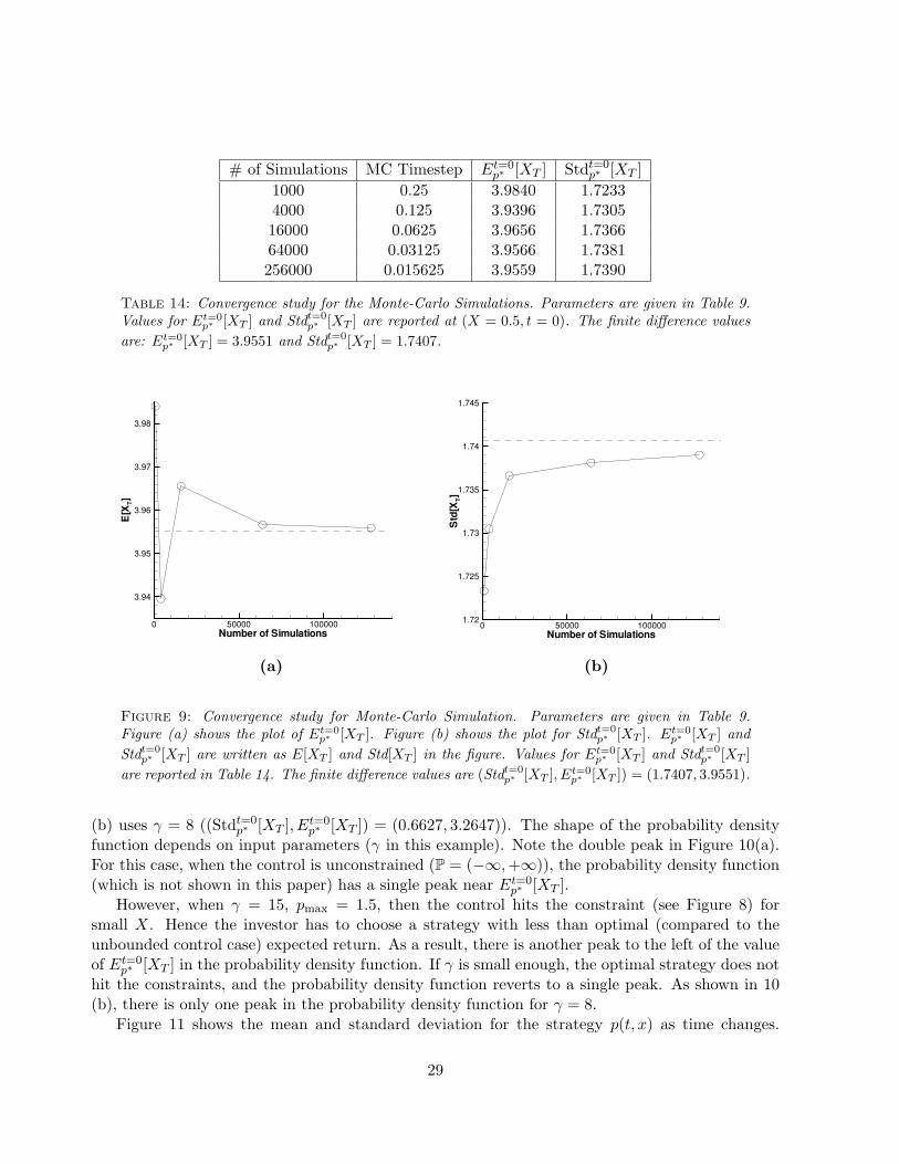
# of Simulations MC Timestep Et=0p∗ [XT ] Stdt=0

p∗ [XT ]1000 0.25 3.9840 1.72334000 0.125 3.9396 1.730516000 0.0625 3.9656 1.736664000 0.03125 3.9566 1.7381256000 0.015625 3.9559 1.7390

Table 14: Convergence study for the Monte-Carlo Simulations. Parameters are given in Table 9.Values for Et=0

p∗ [XT ] and Stdt=0p∗ [XT ] are reported at (X = 0.5, t = 0). The finite difference values

are: Et=0p∗ [XT ] = 3.9551 and Stdt=0

p∗ [XT ] = 1.7407.

Number of Simulations

E[X T]

0 50000 100000

3.94

3.95

3.96

3.97

3.98

Number of Simulations

Std[

X T]

0 50000 1000001.72

1.725

1.73

1.735

1.74

1.745

(a) (b)

Figure 9: Convergence study for Monte-Carlo Simulation. Parameters are given in Table 9.Figure (a) shows the plot of Et=0

p∗ [XT ]. Figure (b) shows the plot for Stdt=0p∗ [XT ]. Et=0

p∗ [XT ] andStdt=0

p∗ [XT ] are written as E[XT ] and Std[XT ] in the figure. Values for Et=0p∗ [XT ] and Stdt=0

p∗ [XT ]are reported in Table 14. The finite difference values are (Stdt=0

p∗ [XT ], Et=0p∗ [XT ]) = (1.7407, 3.9551).

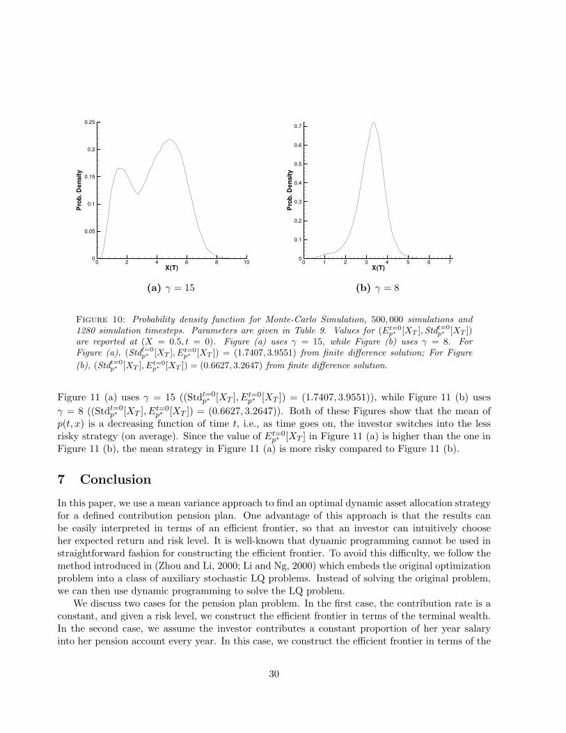
(b) uses γ = 8 ((Stdt=0p∗ [XT ], Et=0

p∗ [XT ]) = (0.6627, 3.2647)). The shape of the probability densityfunction depends on input parameters (γ in this example). Note the double peak in Figure 10(a).For this case, when the control is unconstrained (P = (−∞,+∞)), the probability density function(which is not shown in this paper) has a single peak near Et=0

p∗ [XT ].However, when γ = 15, pmax = 1.5, then the control hits the constraint (see Figure 8) for

small X. Hence the investor has to choose a strategy with less than optimal (compared to theunbounded control case) expected return. As a result, there is another peak to the left of the valueof Et=0

p∗ [XT ] in the probability density function. If γ is small enough, the optimal strategy does nothit the constraints, and the probability density function reverts to a single peak. As shown in 10(b), there is only one peak in the probability density function for γ = 8.

Figure 11 shows the mean and standard deviation for the strategy p(t, x) as time changes.

29

X(T)

Prob

.Den

sity

0 2 4 6 8 100

0.05

0.1

0.15

0.2

0.25

X(T)

Prob

.Den

sity

0 1 2 3 4 5 6 70

0.1

0.2

0.3

0.4

0.5

0.6

0.7

(a) γ = 15 (b) γ = 8

Figure 10: Probability density function for Monte-Carlo Simulation, 500, 000 simulations and1280 simulation timesteps. Parameters are given in Table 9. Values for (Et=0

p∗ [XT ],Stdt=0p∗ [XT ])

are reported at (X = 0.5, t = 0). Figure (a) uses γ = 15, while Figure (b) uses γ = 8. ForFigure (a), (Stdt=0

p∗ [XT ], Et=0p∗ [XT ]) = (1.7407, 3.9551) from finite difference solution; For Figure

(b), (Stdt=0p∗ [XT ], Et=0

p∗ [XT ]) = (0.6627, 3.2647) from finite difference solution.

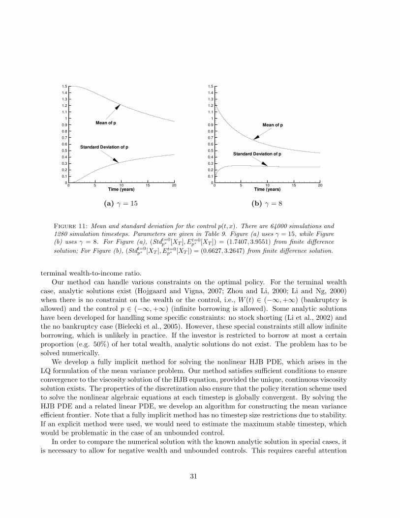
Figure 11 (a) uses γ = 15 ((Stdt=0p∗ [XT ], Et=0

p∗ [XT ]) = (1.7407, 3.9551)), while Figure 11 (b) usesγ = 8 ((Stdt=0

p∗ [XT ], Et=0p∗ [XT ]) = (0.6627, 3.2647)). Both of these Figures show that the mean of

p(t, x) is a decreasing function of time t, i.e., as time goes on, the investor switches into the lessrisky strategy (on average). Since the value of Et=0

p∗ [XT ] in Figure 11 (a) is higher than the one inFigure 11 (b), the mean strategy in Figure 11 (a) is more risky compared to Figure 11 (b).

7 Conclusion

In this paper, we use a mean variance approach to find an optimal dynamic asset allocation strategyfor a defined contribution pension plan. One advantage of this approach is that the results canbe easily interpreted in terms of an efficient frontier, so that an investor can intuitively chooseher expected return and risk level. It is well-known that dynamic programming cannot be used instraightforward fashion for constructing the efficient frontier. To avoid this difficulty, we follow themethod introduced in (Zhou and Li, 2000; Li and Ng, 2000) which embeds the original optimizationproblem into a class of auxiliary stochastic LQ problems. Instead of solving the original problem,we can then use dynamic programming to solve the LQ problem.

We discuss two cases for the pension plan problem. In the first case, the contribution rate is aconstant, and given a risk level, we construct the efficient frontier in terms of the terminal wealth.In the second case, we assume the investor contributes a constant proportion of her year salaryinto her pension account every year. In this case, we construct the efficient frontier in terms of the

30

Time (years)0 5 10 15 200

0.10.20.30.40.50.60.70.80.9

11.11.21.31.41.5

Mean of p

Standard Deviation of p

Time (years)0 5 10 15 200

0.10.20.30.40.50.60.70.80.9

11.11.21.31.41.5

Mean of p

Standard Deviation of p

(a) γ = 15 (b) γ = 8

Figure 11: Mean and standard deviation for the control p(t, x). There are 64000 simulations and1280 simulation timesteps. Parameters are given in Table 9. Figure (a) uses γ = 15, while Figure(b) uses γ = 8. For Figure (a), (Stdt=0

p∗ [XT ], Et=0p∗ [XT ]) = (1.7407, 3.9551) from finite difference

solution; For Figure (b), (Stdt=0p∗ [XT ], Et=0

p∗ [XT ]) = (0.6627, 3.2647) from finite difference solution.

terminal wealth-to-income ratio.Our method can handle various constraints on the optimal policy. For the terminal wealth

case, analytic solutions exist (Hojgaard and Vigna, 2007; Zhou and Li, 2000; Li and Ng, 2000)when there is no constraint on the wealth or the control, i.e., W (t) ∈ (−∞,+∞) (bankruptcy isallowed) and the control p ∈ (−∞,+∞) (infinite borrowing is allowed). Some analytic solutionshave been developed for handling some specific constraints: no stock shorting (Li et al., 2002) andthe no bankruptcy case (Bielecki et al., 2005). However, these special constraints still allow infiniteborrowing, which is unlikely in practice. If the investor is restricted to borrow at most a certainproportion (e.g. 50%) of her total wealth, analytic solutions do not exist. The problem has to besolved numerically.

We develop a fully implicit method for solving the nonlinear HJB PDE, which arises in theLQ formulation of the mean variance problem. Our method satisfies sufficient conditions to ensureconvergence to the viscosity solution of the HJB equation, provided the unique, continuous viscositysolution exists. The properties of the discretization also ensure that the policy iteration scheme usedto solve the nonlinear algebraic equations at each timestep is globally convergent. By solving theHJB PDE and a related linear PDE, we develop an algorithm for constructing the mean varianceefficient frontier. Note that a fully implicit method has no timestep size restrictions due to stability.If an explicit method were used, we would need to estimate the maximum stable timestep, whichwould be problematic in the case of an unbounded control.

In order to compare the numerical solution with the known analytic solution in special cases, itis necessary to allow for negative wealth and unbounded controls. This requires careful attention

31

to the grid construction and form of the control as the mesh and timesteps shrink to zero.Numerical tests show that our numerical solutions converge to the analytic solution (where

available). The policy iteration scheme converges very rapidly. We also examine some cases ofrealistic constraints where analytic solutions do not exist. From a practical point of view, weobserve that the addition of realistic constraints can completely alter some of the properties ofthe mean variance solution compared to the unconstrained control case. For example, the efficientfrontier is no longer a straight line, the frontier is sensitive to the risky asset volatility, and the 80%rule (Li and Zhou, 2006) no longer holds.

We plan to carry out a similar study of time-consistent mean variance optimal asset allocationin the near future.

A Discrete Equation Coefficients

Let pni denote the optimal control p∗ at node i, time level n and set

an+1i = a(zi, , p

ni ), bn+1

i = b(zi, , pni ), cn+1

i = c(zi, , pni ) . (A.1)

Then, we can use central, forward or backward differencing at any node.Central Differencing:

αni,central =

[2an

i

(zi − zi−1)(zi+1 − zi−1)− bn

i

zi+1 − zi−1

]βn

i,central =[

2ani

(zi+1 − zi)(zi+1 − zi−1)+

bni

zi+1 − zi−1

]. (A.2)

Forward/backward Differencing: (bni > 0/ bn

i < 0)

αni,forward/backward =

[2an

i

(zi − zi−1)(zi+1 − zi−1)+ max(0,

−bni

zi − zi−1)]

βni,forward/backward =

[2an

i

(zi+1 − zi)(zi+1 − zi−1)+ max(0,

bni

zi+1 − zi)]

. (A.3)

References

Barles, G. (1997). Convergence of numerical schemes for degenerate parabolic equations arisingin finance. In L. C. G. Rogers and D. Talay (Eds.), Numerical Methods in Finance, pp. 1–21.Cambridge University Press, Cambridge.

Barles, G. and J. Burdeau (1995). The Dirichlet problem for semilinear second-order degenerateelliptic equations and applications to stochastic exit time control problems. Communications inPartial Differential Equations 20, 129–178.

Barles, G., C. Daher, and M. Romano (1995). Convergence of numerical shemes for parabolicequations arising in finance theory. Mathematical Models and Methods in Applied Sciences 5,125–143.

32

Barles, G. and E. Jakobsen (2005). Error bounds for monotone approximation schemes for parabolicHamilton-Jacobi-Bellman equations. Working Paper, Norwegian University of Science and Tech-nology.

Barles, G. and E. Rouy (1998). A strong comparison result for the Bellman equation arising instochastic exit time control problems and applications. Communications in Partial DifferentialEquations 23, 1945–2033.

Barles, G. and P. Souganidis (1991). Convergence of approximation schemes for fully nonlinearequations. Asymptotic Analysis 4, 271–283.

Basak, S. and G. Chabakauri (2007). Dynamic mean-variance asset allocation. Working Paper,London Business School.

Bielecki, T., J. H, S. Pliska, and X. Zhou (2005). Continuous time mean-variance portfolio selectionwith bankruptcy prohibition. Mathematical Finance 15, 213–244.

Cairns, A., D. Blake, and K. Dowd (2006). Stochastic lifestyling: optimal dynamic asset allocationfor defined contribution pension plans. Journal of Economic Dynamics and Control 30, 843–877.

Chaumont, S. (2004). A strong comparison result for viscosity solutions to Hamilton-Jacobi-Bellman equations with Dirichlet conditions on a non-smooth boundary. Working paper, InstituteElie Cartan, Universite Nancy I.

Chen, Z. and P. Forsyth (2008). A numerical scheme for the impulse control formulation forpricing variable annuities with a guaranteed minimum withdrawal benefit (GMWB). NumerischeMathematik 109, 535–569.

Chiu, M. and D. Li (2006). Asset and liability management under a continuous time mean varianceoptimization framework. Insurance: Mathematics and Economics 39, 330–355.

Crandall, M. G., H. Ishii, and P. L. Lions (1992). User’s guide to viscosity solutions of second orderpartial differential equations. Bulletin of the American Mathematical Society 27, 1–67.

Duffie, D. and H. Richardson (1991). Mean variance hedging in continuous time. Annals of AppliedProbability 1, 1–15.

Forsyth, P. A. and G. Labahn (2008). Numerical methods for controlled Hamilton-Jacobi-BellmanPDEs in finance. Journal of Computational Finance 11 (Winter), 1–44.

Gerrard, R., S. Haberman, and E. Vigna (2004). Optimal investment choices post retirement in adefined contribution pension scheme. Insurance: Mathematics and Economics 35, 321–342.

Hojgaard, B. and E. Vigna (2007). Mean variance portfolio selection and efficient frontier fordefined contribution pension schemes. Working Paper, Aalborg University.

Kahl, C., M. Gunther, and T. Rossberg (2008). Structure preserving stochastic integration schemesin interest rate derivative modelling. Applied Numerical Mathematics 58, 284–295.

33

Leippold, M., F. Trojani, and P. Vanini (2004). A geometric approach to multiperiod mean varianceoptimization of assets and liabilities. Journal of Economic Dynamics and Control 28, 1079–1113.

Li, D. and W.-L. Ng (2000). Optimal dynamic portfolio selection: Multiperiod mean varianceformulation. Mathematical Finance 10, 387–406.

Li, X. and X. Y. Zhou (2006). Continuous time mean variance efficiency and the 80% rule. Annalsof Applied Probability 16, 1751–1763.

Li, X., X. Y. Zhou, and E. B. Lim (2002). Dynamic mean variance portfolio selection with no-shorting constraints. SIAM Journal on Control and Optimization 40, 1540–1555.

Lorenz, J. and R. Almgren (2007). Adaptive arrival price. in Algorithmic Trading III: Precision,Control, Execution, Brian R. Bruce, editor, Institutional Investor Journals.

Merton, R. (1971). Optimum consumption and portfolio rules in a continuous time model. Journalof Economics Theory 3, 373–413.

Nguyen, P. and R. Portrai (2002). Dynamic asset allocation with mean variance preferences and asolvency constraint. Journal of Economic Dynamics and Control 26, 11–32.

Pooley, D., P. Forsyth, and K. Vetzal (2003). Numerical convergence properties of option pricingPDEs with uncertain volatility. IMA Journal of Numerical Analysis 23, 241–267.

Wang, J. and P. Forsyth (2008). Maximal use of central differencing for Hamilton-Jacobi-BellmanPDEs in finance. SIAM Journal on Numerical Analysis 46, 1580–1601.

Wang, Z., J. Xia, and L. Zhang (2007). Optimal investment for the insurer: The martingaleapproach. Insurance: Mathematics and Economics 40, 322–334.

Zhou, X. and D. Li (2000). Continuous time mean variance portfolio selection: A stochastic LQframework. Applied Mathematics and Optimization 42, 19–33.

34