numerical solution of the wave equation in unbounded domains
TRANSCRIPT

Institut für MathematikUniversität Zürich
Masterarbeit
Numerical Solution of the Wave Equation inUnbounded Domains
Martin Huber
ausgeführt unter der Leitung von
Prof. Dr. Stefan Sauter
undAlexander Veit
Zürich, im März 2011

Contents
1 Introduction 1
2 Formulation of the Problem 3
3 Mathematical Framework 7
3.1 Discrete Fourier Transform . . . . . . . . . . . . . . . . . . . . . . . . . . . . 7
3.2 Fourier Transform . . . . . . . . . . . . . . . . . . . . . . . . . . . . . . . . . 8
3.3 Laplace Transform . . . . . . . . . . . . . . . . . . . . . . . . . . . . . . . . . 9
3.4 Sobolev Spaces . . . . . . . . . . . . . . . . . . . . . . . . . . . . . . . . . . . 11
3.4.1 Sobolev Spaces of Integer Order on Domains . . . . . . . . . . . . . . 11
3.4.2 Sobolev Spaces Hs(Ω), for s ∈ R≥0 . . . . . . . . . . . . . . . . . . . . 12
3.4.3 Sobolev Spaces on Surfaces . . . . . . . . . . . . . . . . . . . . . . . . 13
3.4.4 Traces, Liftings and Extensions . . . . . . . . . . . . . . . . . . . . . . 14
3.4.5 Dual Spaces of Sobolev Spaces . . . . . . . . . . . . . . . . . . . . . . 15
3.4.6 Sobolev Spaces for Problems in Time and Space . . . . . . . . . . . . 15
3.5 Weak Formulation of Equations . . . . . . . . . . . . . . . . . . . . . . . . . . 16
3.6 Derivation of the Convolution Quadrature . . . . . . . . . . . . . . . . . . . . 18
3.7 Derivation of BDF2 . . . . . . . . . . . . . . . . . . . . . . . . . . . . . . . . . 21
3.8 Spherical Harmonics . . . . . . . . . . . . . . . . . . . . . . . . . . . . . . . . 22
4 Theory for the Exact Problem 23
4.1 Properties of the Wave Equation . . . . . . . . . . . . . . . . . . . . . . . . . 23
4.2 Existence and Uniqueness for the full space Problem . . . . . . . . . . . . . . 24
4.3 Motivation for the Single Layer Potential . . . . . . . . . . . . . . . . . . . . . 24
4.4 Connection to the Helmholtz Equation . . . . . . . . . . . . . . . . . . . . . . 25
4.5 Theory for the Helmholtz Problem . . . . . . . . . . . . . . . . . . . . . . . . 26
4.6 Properties of the Single Layer Potential . . . . . . . . . . . . . . . . . . . . . 28
4.7 Existence and Uniqueness for the Single Layer Potential . . . . . . . . . . . . 30
5 Numerical Discretisation 35
5.1 Time Discretisation . . . . . . . . . . . . . . . . . . . . . . . . . . . . . . . . . 35
5.2 Space Discretisation . . . . . . . . . . . . . . . . . . . . . . . . . . . . . . . . 36
5.2.1 Surface Paneling . . . . . . . . . . . . . . . . . . . . . . . . . . . . . . 36
5.2.2 Piecewise Constant Boundary Elements . . . . . . . . . . . . . . . . . 38
5.2.3 Piecewise Linear Boundary Elements . . . . . . . . . . . . . . . . . . . 38
5.2.4 Discretisation for a Given Basis . . . . . . . . . . . . . . . . . . . . . . 39
5.3 Approximation of the Convolution Weights . . . . . . . . . . . . . . . . . . . 41
5.4 Decoupling the Systems . . . . . . . . . . . . . . . . . . . . . . . . . . . . . . 42
5.5 Approximation of the Wave Function . . . . . . . . . . . . . . . . . . . . . . . 44
I
II CONTENTS
6 Theory for the Discretised Problem 47
6.1 Boundary Element Space . . . . . . . . . . . . . . . . . . . . . . . . . . . . . 476.2 Approximation of the Convolution Weights . . . . . . . . . . . . . . . . . . . 476.3 Convergence of the Method . . . . . . . . . . . . . . . . . . . . . . . . . . . . 48
7 MATLAB Implementation 51
7.1 Algorithm . . . . . . . . . . . . . . . . . . . . . . . . . . . . . . . . . . . . . . 517.2 Generating a Mesh . . . . . . . . . . . . . . . . . . . . . . . . . . . . . . . . . 537.3 Data Structures for Mesh Handling and Global Parameters . . . . . . . . . . 537.4 Numerical Integration . . . . . . . . . . . . . . . . . . . . . . . . . . . . . . . 587.5 Routines . . . . . . . . . . . . . . . . . . . . . . . . . . . . . . . . . . . . . . . 61
7.5.1 Arranging the Pairs of Triangles . . . . . . . . . . . . . . . . . . . . . 627.5.2 Calculating the System Matrices . . . . . . . . . . . . . . . . . . . . . 627.5.3 Calculating the Right-Hand Side Vectors . . . . . . . . . . . . . . . . . 637.5.4 Implementing the Scaled Fourier Transform . . . . . . . . . . . . . . . 657.5.5 Calculating the Solution of the Wave Equation . . . . . . . . . . . . . 657.5.6 Description of the Routines . . . . . . . . . . . . . . . . . . . . . . . . 66
7.6 Storage Costs . . . . . . . . . . . . . . . . . . . . . . . . . . . . . . . . . . . . 71
8 Numerical Tests 73
8.1 Test Case with known Analytical Solution . . . . . . . . . . . . . . . . . . . . 738.2 Error Measure . . . . . . . . . . . . . . . . . . . . . . . . . . . . . . . . . . . . 738.3 Convergence Tests . . . . . . . . . . . . . . . . . . . . . . . . . . . . . . . . . 74
8.3.1 Piecewise Constant Elements . . . . . . . . . . . . . . . . . . . . . . . 768.3.2 Piecewise Linear Elements . . . . . . . . . . . . . . . . . . . . . . . . . 78
8.4 Complexity Tests . . . . . . . . . . . . . . . . . . . . . . . . . . . . . . . . . . 798.5 Acoustic Tests . . . . . . . . . . . . . . . . . . . . . . . . . . . . . . . . . . . . 84
9 Conclusion 87
Chapter 1
Introduction
Wave propagation is a fundamental process in nature. Hence the concept of waves arises inseveral disciplines of physics, although the physical processes, which are modeled by waves,dier fundamentally. On the one hand there are mechanical waves like water waves or acousticwaves, which are bounded to a medium, and on the other hand electromagnetic waves, likevisible light or radio waves, that propagate even in the vacuum. Furthermore, the concept ofwaves is also used in quantum mechanics, as matter waves, as well as in the general theoryof relativity, where gravitational waves are predicted. The common property of wave prop-agation is the transport of energy through the space without transporting any mass. Thistransport is obtained by a time dependent conversion of two physical quantities, e.g. kineticand potential energy in the case of mechanical waves.
In the eld of research of acoustics the scattering of acoustic waves at an obstacle is a commonproblem. A classical domain of that research is the analysis of the acoustics of buildings, e.g.operas, theaters or churches. In these buildings acoustic waves produced by human voice ormusical instruments are supposed to reach the listeners as well as it is possible. The contraryintention governs in the domain of noise barriers, where scattering problems directly aectthe everyday life. To protect residential areas eciently and cost-eectively against noise,various tests about the placement and the materials of the barriers are necessary. Moreover,the problem of scattered waves arises as well in other domains, such as electromagnetic wavesin the sonar technology, where conversely the scattered wave is received and the original wavehas to be determined. Therefore, the investigation of incoming waves scattered at an obstacledelivers insights into various problems arising in applied sciences.
Examining the space where the investigated wave propagates often reveals that this spaceis an unbounded domain in the three dimensional space, e.g. for acoustic waves in the caseof ancient outdoor theaters or noise calculations. Hence, ecient methods for the numericalsolution of the wave equation in unbounded domains are needed. Discretizing an unboundeddomain for applying a method, which is based on classical nite elements (FEM), leads toseveral problems, as the boundary at innity somehow has to be modeled. Thus the ap-proach presented in [BS08], that is based on an integral equation involving just the compactboundary of the scatterer, is applied in this thesis. This integral equation then is resolvedwith respect to the space by a boundary element method (BEM). That reduces the spatialdimension of the domains by one dimension, as surfaces and not volumes in R3 arise as originof the discretisation, which will lead to an essential reduction of the costs of calculations.
The goal of this thesis is to implement a method based on the convolution quadrature withconstant step size in time and a Galerkin boundary element method in space as presentedin [BS08] and its precedent papers [HKS09] resp. [HKS07]. The calculation of the solution
1
2 CHAPTER 1. INTRODUCTION
in the exterior domain is divided into two parts: The main part is the numerical solutionof an integral equation. In order to reduce the amount of time needed for the calculation,a special approximation of some convolution weights is applied that will reduce the problemto decoupled Helmholtz problems which can be computed parallelly. The Galerkin boundaryelement method, applied on the weak formulation of a Helmholtz problem, gives rise to inte-grals of a singular kernel on the domain of the Cartesian product of two surface panels. Tocalculate these integrals, a specialized quadrature developed in [SS04], based on a tensorisedGauss-quadrature, is applied. This rst part will provide an approximation of the unknowndensity determining the solution in the exterior domain. This solution then is calculated inthe second part by evaluating an integral representation including the provided density. Thisimplementation will allow the calculation of the scattering of an incoming wave at a soundsoft bounded obstacle in the three dimensional space.
The outline of this thesis is as follows. In Chapter 2 the homogeneous exterior Dirichlet prob-lem is deduced and the basic approach by a retarded single layer potential is introduced. Solv-ing that problem theoretically and numerically needs several concepts and methods. Theseare presented in a compact manner in Chapter 3 and include topics like Laplace transform,Sobolev spaces on domains and surfaces as well as the derivation of the convolution quadra-ture and the linear multistep method BDF2.
In a second step in Chapter 4, the properties of the wave equation and its solution are ex-amined. This also involves physical principles and an integral representation of the solutionof the wave equation. This motivates the chosen approach by a retarded potential, whoseproperties are investigated consecutively. Applying the Laplace transform on a solution ofthe wave equation will show the strong link to the Helmholtz equation. As the Laplace trans-form of an integral kernel also is fundamental in the convolution quadrature, this connectionis the basis for any existence and uniqueness result. A calculus presented in [Lub94] allowsthe transfer of the results obtained for the Helmholtz equation back to the wave equation,resulting in the theorem about existence and uniqueness for the retarded potential approach.
In Chapter 5 the numerical discretisation of the homogeneous exterior Dirichlet problem ispresented. First of all the time discretisation via the convolution quadrature is introduced.After the denition of the boundary element spaces, restricted to the case of discontinuouspiecewise constant resp. continuous piecewise linear elements, the Galerkin boundary elementmethod can be established. Both discretisations together result in a Toeplitz system, which isdecoupled by applying a Fourier style approximation of the convolution weights. In addition,the framework for the calculation of the exterior solution is given based on a linear interpola-tion in time. The existence, convergence and stability results for that presented discretisationis then stated in Chapter 6.
The main part of this thesis builds a MATLAB implementation of the introduced discreti-sation scheme, which is presented in Chapter 7 in detail. This includes the description ofdata structures and routines along with details about the quadrature methods. Furthermore,the complexity of the implementation is examined. As last step, the implementation is val-idated by checking the predicted convergence rates. For this purpose an error measure isdeveloped and Dirichlet boundary conditions are presented, where the analytical solution isknown exactly.
Chapter 2
Formulation of the Problem
This chapter is dedicated to the formulation and the motivation of the mathematical problemthat we want to solve. The goal is to introduce it in a short but clear manner without anyfurther theory, as that will be presented in the subsequent chapters.
Let Ω := Ωe ⊂ R3 be an unbounded connected Lipschitz domain, called the exterior domain,with bounded complement Ωi := R3\Ωe, the interior domain, and therefore bounded, compactboundary Γ := ∂Ω. Assume that the inhomogeneity f : Ω× (0, T )→ R and the initial valuesu0, u1 : Ω→ R are given. Consider now the following exterior scattering problem
∂2t u(x, t)−∆u(x, t) = f(x, t) in Ω× (0, T ) (2.1a)
u(x, 0) = u0(x) ∀x ∈ Ω (2.1b)
∂tu(x, 0) = u1(x) ∀x ∈ Ω (2.1c)
u(x, t) = 0 on Γ× (0, T ), (2.1d)
for a xed end time T > 0. That original problem, given by (2.1) and called Porig, is aninhomogeneous exterior Dirichlet problem.
To get a boundary integral equation, we have to reduce Porig to a homogeneous problem.That is achieved by splitting the wave function u into a part consisting of the incident waveuinc and a part consisting of the scattered wave usca. For uinc arises then the problem
∂2t uinc(x, t)−∆uinc(x, t) = f(x, t) in R3 × (0, T ) (2.2a)
uinc(x, 0) = u0(x) ∀x ∈ R3 (2.2b)
∂tuinc(x, 0) = u1(x) ∀x ∈ R3, (2.2c)
where f , u0 and u1 are prolongations of f , u0, u1 to the full space R3 in the sense of Section3.4.4. This problem for the incident wave dened by (2.2) is denoted by Pinc and is a so calledCauchy problem for the wave equation on the full space.
Given a solution of Pinc called uinc, whose existence is discussed in Section 4.2, we are able toformulate the homogeneous exterior Dirichlet problem arising for usca
∂2t usca(x, t)−∆usca(x, t) = 0 in Ω× (0, T ) (2.3a)
usca(x, 0) = 0 ∀x ∈ Ω (2.3b)
∂tusca(x, 0) = 0 ∀x ∈ Ω (2.3c)
usca(x, t) = −uinc(x, t) on Γ× (0, T ), (2.3d)
denoted as Psca. The goal of this thesis is to develop an ecient numerical solver for thisproblem. Merging the results of Pinc and Psca leads to the solution for Porig by taking thesuperposition u(x, t) := uinc(x, t) + usca(x, t).
3
4 CHAPTER 2. FORMULATION OF THE PROBLEM
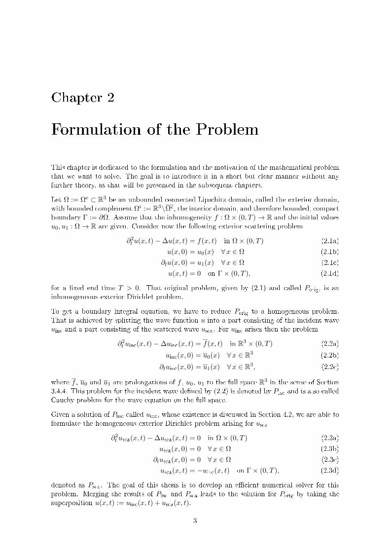
As the interests of this thesis are focused on the scattering of an incoming wave by an obstacleand not on the propagation nor the formation of a wave in the full space, the problem Pinc willnot be considered in the numerical examples. We restrict ourselves to the case of a transientwave uinc, i.e. uinc satises Pinc with f ≡ 0 in Ω× (0, T ) and uinc vanishes in a neighbourhoodof Ωi at t = 0. That problem has its application for example in acoustics.
Ωi
Ωe
uinc
usca
usca
usca
Figure 2.1: Scattering of an incoming wave by an obstacle
It models a scattering problem with an obstacle occupying Ωi and placed into a homogeneousmedium, e.g. uids or air, that covers the unbounded exterior domain Ωe. At the time t = 0,a neighbourhood of the obstacle is not perturbed by any acoustic pressure. A wave uinc, thatarises from the far eld, propagates with nite velocity and without any disturbance onto theobstacle. Starting at the point, where the incoming wave reaches the obstacle, a scatteredwave appears, as the obstacle reects some parts of the incoming wave. The amount, which isreected, depends on the material properties of the obstacle. In the studied case the obstacleis a soft scatterer, which is modeled by imposing Dirichlet conditions on the boundary Γ. Thecases of a hard resp. absorbing scatterer would be modeled by Neumann resp. absorbingboundary conditions (cf. [HD03]).
After that motivation by acoustics, we rewrite the problem Psca with simpler notation as
∂2t u(x, t)−∆u(x, t) = 0 in Ω× (0, T ) (2.4a)
u(x, 0) = 0 ∀x ∈ Ω (2.4b)
∂tu(x, 0) = 0 ∀x ∈ Ω (2.4c)
u(x, t) = g(x, t) on Γ× (0, T ), (2.4d)
for a given g on Γ× (0, T ) and call it P for further reference.
Motivated by the results of classical electromagnetic theory (cf. Section 4.3), we employ a
5
single layer potential ansatz for the unknown solution u
(Sϕ)(x, t) :=
∫ t
0
∫Γk(x− y, t− τ)ϕ(y, τ)dΓydτ, (2.5)
to solve the problem P . The distributional k is given by the fundamental solution of the waveequation (cf. Section 4.6)
k(z, s) =δ(‖z‖ − s)
4π‖z‖. (2.6)
Any u := Sϕ solves P with the exception of the boundary condition (2.4d) (cf. Section 4.6).Using the continuity (ibid.) of the single layer potential as Ω 3 x → Γ the inner integral ofthe right-hand side in (2.5) has to be understood as an improper Riemann integral
(V ϕ)(x, t) :=
∫ t
0
∫Γk(x− y, t− τ)ϕ(y, τ)dΓydτ (x, t) ∈ Γ× (0, T ). (2.7)
To fulll the boundary condition (2.4d) the integral equation
V ϕ = g on Γ× (0, T ). (2.8)
has to be solved. At the core of this thesis a method to solve this retarded potential integralequation numerically is developed.

6 CHAPTER 2. FORMULATION OF THE PROBLEM

Chapter 3
Mathematical Framework
During the development of the theoretical background and the numerical discretisation, vari-ous mathematical concepts are used. The aim of this chapter is to provide the analytic toolswhich later will be employed for the mathematical analysis for the retarded potential integralequation. For the proofs and further results we will give reference to the literature.
3.1 Discrete Fourier Transform
By approximating an integral of the form of the Cauchy integral formula by using the trape-zoidal rule on a circle, the arising summation can be regarded as a certain formulation ofthe discrete Fourier transform. The goal is to provide the way on which it can be reducedto the discrete Fourier transform, in order to use the Fast Fourier Transform (FFT) for theimplementation. Further theory and results can be found in [Hen86].
Given a vector a = (a0, . . . , aN ) ∈ CN+1, N ∈ N the discrete Fourier transform a =(a0, . . . , aN ) ∈ CN+1 is dened by
ak =
N∑j=0
ajζjkN+1, (3.1)
for k = 0, . . . , N and ζN+1 := e−2πiN+1 . To reconstruct a from a, one can apply the inverse
transform
ak =1
N + 1
N∑j=0
ajζ−jkN+1, k = 0, . . . , N. (3.2)
Let k ∈ 0, . . . , N and λ ∈ R>0. Consider the discrete Fourier transform of the vectorb = (λ0a0, . . . , λ
NaN ), which is the result of a special scaling of the vector a,
bk =
N∑j=0
bjζjkN+1 =
N∑j=0
λjajζjkN+1. (3.3)
Written in terms of a it holds
λkak = bk =1
N + 1
N∑j=0
bjζ−jkN+1 =⇒ ak =
λ−k
N + 1
N∑j=0
bjζ−jkN+1. (3.4)
This motivates the denition of a scaled discrete Fourier transform. The original Fouriertransform is obtained for λ = 1.
7
8 CHAPTER 3. MATHEMATICAL FRAMEWORK
Denition 3.1.1. For a vector a = (a0, . . . , aN ) ∈ CN+1 and given parameter λ > 0 the
scaled discrete Fourier transform is dened by
ak =
N∑j=0
λjajζjkN+1. (3.5)
Lemma 3.1.2. The inverse of the scaled discrete Fourier transform is given by
ak =λ−k
N + 1
N∑j=0
ajζ−jkN+1. (3.6)
Remark 3.1.3. This derivation shows that the scaled discrete Fourier transform can beimplemented by using the fast Fourier transform and by scaling the argument resp. the resultby the matrix Λ resp. its inverse, with
Λ :=
λ0
λ1 0λ2
0. . .
λN
. (3.7)
3.2 Fourier Transform
In this section we will sketch some fundamentals of the Fourier transform. For further resultsand applications we refer to [SS03].
Denition 3.2.1. To express high order multidimensional derivation, it is convenient to use
multi-indices. Let α ∈ Nn be a multi-index. Dene the following quantities
|α| :=n∑i=1
αi, vα :=
n∏i=1
vαii with v ∈ Cn, Dαf(x) := Dαxf(x) :=
∂|α|f(x)
∂α1x1 · · · ∂αnxn
. (3.8)
Next we dene the functional space used for the Fourier transform.
Denition 3.2.2. A function f : Rn → C is called rapidly decreasing if
supx∈Rn
|xαf(x)| <∞ ∀α ∈ Nn. (3.9)
The space containing all indenitely dierentiable functions f : Rn → C with
supx∈Rn
∣∣∣xαDβf(x)∣∣∣ <∞ ∀α, β ∈ Nn, (3.10)
is the Schwartz space S(Rn).
For any f ∈ S(Rn) all its derivatives are rapidly decreasing. Let us dene now the Fouriertransform for a function f ∈ S(Rn)
Denition 3.2.3. For u ∈ S(Rn) the Fourier transform Fu : Rn → C is dened by
(Fu)(ξ) := (2π)−n2
∫Rne−i ξ·xu(x)dx, (3.11)
where · in the expression ξ · x denominates the Euclidean scalar product on Rn.
3.3. LAPLACE TRANSFORM 9
Next we will recall the formula of Plancherel and the inverse Fourier transform.
Theorem 3.2.4. For a function u ∈ S(Rn), it holds that the L2-norm is preserved by the
Fourier transform ∫Rn|(Fu)(ξ)|2dξ =
∫Rn|u(x)|2dx. (3.12)
Furthermore the inverse mapping F−1, for a v ∈ S(Rn), is given by
(F−1v)(x) := (2π)−n2
∫Rnei x·ξv(ξ)dξ, (3.13)
i.e. F−1(Fu) = u for all u ∈ S(Rn).
We conclude that the Fourier transform F is a bijective isometry of S(Rn) onto itself. TheFourier transform has several important properties. Fundamental is the property concerningthe transformation of derivatives.
Lemma 3.2.5.
F(Dαu)(ξ) = i|α|ξα(Fu)(ξ) ∀u ∈ S(Rn). (3.14)
This is one of the reasons that the Fourier transform, and later on the Laplace transform,is often used in the context of partial dierential equations, as the derivative of a functionbecomes a simple multiplication in the Fourier image. Therefore it is often simpler to solve afull space problem in the Fourier image and then transform the result back using the inverseFourier transform.
As we have seen, the Fourier transform preserves the L2-norm. Furthermore the test functionsC∞0 (Rn), dened in Denition 3.4.1, are a subspace of the Schwartz space S(Rn) and lie densein L2(Rn). Consequently we may extend the Fourier transform to Sobolev spaces, which willbe dened in Section 3.4.1. That is done for example in [Hac92, Section 6.2.3]. We just quotethe main result.
Theorem 3.2.6. F and F−1 are isometric mappings of L2(Rn) onto itself. The scalar productsatises
(u, v)L2 = (Fu,Fv)L2 ∀u, v ∈ L2(Rn). (3.15)
The theory of the Fourier transform can be extended to tempered distributions, denoted byS ′(Rn), the dual space of S(Rn), i.e. the continuous, linear functions on S(Rn). This theoryis developed, e.g., in [Jan71].
3.3 Laplace Transform
As we will see later, the discretisation with relation to the time strongly relies on the Laplacetransform of the distributional integral kernel k. The Laplace transform itself can be inter-preted as a Fourier transform for special functions.
Denition 3.3.1. Let f be a function f : R→ R with f(t) = 0 for t ∈ (−∞, 0), i.e. a causal
function. f is Laplace transformable on the half-plane s ∈ C | Re (s) > σ0 if there exists aσ0 ∈ R, such that e−σ0tf(t) ∈ S(R) i.e. is Fourier transformable.
10 CHAPTER 3. MATHEMATICAL FRAMEWORK
Denition 3.3.2. For a Laplace transformable function f : R→ R and σ0 chosen as Deni-
tion 3.3.1, the Laplace transform is dened by
f(s) := (Lf)(s) :=
∫ ∞0
f(t)e−stdt, (3.16)
for s ∈ C with Re (s) > σ0.
Using the strong connection to the Fourier transform, the inverse Laplace transform can bedetermined.
Lemma 3.3.3. Let f be Laplace transformable and σ0 ∈ R as in Denition 3.3.1. Then, the
Laplace inversion formula holds
f(t) = (L−1f)(t) :=1
2πi
∫σ+iR
f(s)estds, t ∈ R, σ > σ0. (3.17)
Similarly as for the Fourier transform, there exists a formula for the Laplace transform of thederivatives of a function. Again the derivatives are turned into a polynomial expression whichmakes the Laplace transform suitable for partial dierential equations that follow a certaincausality.
Theorem 3.3.4. Let n ∈ N. For a Laplace transformable function f : R→ R, which is smoothenough, it holds
(Lf (n))(s) = snf(s)−n−1∑k=0
sn−k−1f (k)(0). (3.18)
Another important property is also inherited from the Fourier transform. It is the rule con-cerning the Laplace transform of a convolution.
Denition 3.3.5. Let f ∈ C∞(R), g ∈ C∞0 (R). The convolution f, g : R→ R of f and g is
dened by
(f ∗ g)(x) :=
∫Rf(x− y)g(y)dy, ∀x ∈ R. (3.19)
Theorem 3.3.6. For the convolution of two Laplace transformable functions f, g : R→ R it
holds
(L(f ∗ g))(s) = f(s) · g(s). (3.20)
The theory for the Laplace transform can be extended to distributions. The basic propertiesand the rules, as it can be found, e.g., in [Jan71, Chapter 12], remain the same. Therefore,we apply L to the fundamental solution of the wave equation k, which is a fundamental stepoften used in this thesis. Let us take k(d, t) = δ(d−t)
4πd , the fundamental solution of the waveequation, and calculate its Laplace transform with respect to t. Let be d > 0 and s ∈ C, thenit holds
k(d, s) =
∫ ∞0
e−stk(d, t)dt =1
4πd
∫ ∞0
e−stδ(d− t)dt (3.21)
=e−sd
4πd, (3.22)
which is the fundamental solution of the Helmholtz equation, as we will see in Section 4.5.
3.4. SOBOLEV SPACES 11
3.4 Sobolev Spaces
To solve partial dierential equations, one has to prescribe appropriate function spaces for itssolution. For the boundary integral equation given by (2.8) in the formulation of the problem(cf. Chapter 2) the natural spaces for the proper formulation of existence, uniqueness andwell-posedness results are certain Sobolev spaces. The introduction of the Sobolev Spaces ondomains and surfaces can be found, e.g., in [SS04, Chapter 2.3] and [Hac92, Chapter 6]. Thesubsection about Sobolev Spaces on Banach Spaces is inspired by [Eva98, Section 5.9.2].
3.4.1 Sobolev Spaces of Integer Order on Domains
Let Ω ⊂ Rd be an open set. The starting point for the theory of Sobolev spaces is the Hilbertspace L2(Ω) dened by
L2(Ω) := u : Ω→ C |u Lebesgue measurable and
∫Ω|u|2dx <∞, (3.23)
with its scalar product (u, v)0,Ω := (u, v)L2(Ω) :=∫
Ω u(x)v(x)dx. The associated norm isdenoted as ‖u‖0,Ω or ‖u‖L2(Ω). As usual two functions are identied with each other if theyare equal up to a set of measure zero.
An important role play the spaces of test functions which are used for various denitions andproofs using an appropriate density argument.
Denition 3.4.1. Let Ω ⊂ Rn be an open domain. Dene the following sets of functions
C∞(Ω) := u : Ω→ C |u(k) exists and is continuous ∀ k ∈ N (3.24)
C∞0 (Ω) := u ∈ C∞(Ω) | suppu ⊂⊂ Ω, (3.25)
with suppu := x ∈ Ω |u(x) 6= 0 and Ω′ ⊂⊂ Ω :⇐⇒ Ω′ is a compact subset of Ω.
The reason for the importance of these spaces of test functions is the fact that both aredense in L2(Ω) and therefore, any function f ∈ L2(Ω) can be approximated by innitelydierentiable functions, even with compact support in Ω.
As functions in L2(Ω) in general are not dened in a pointwise sense, one has to introduce amore general notion of derivative in this space, the weak derivative.
Denition 3.4.2. A function u ∈ L2(Ω) has a α-th weak derivative g := Dαu ∈ L2(Ω),α ∈ Nd, if
(g, v)0,Ω = (−1)|α|(u,Dαv)0,Ω ∀ v ∈ C∞0 (Ω). (3.26)
Denition 3.4.3. Let Ω ⊂ Rd be a domain. For k ∈ N the Sobolev space Hk(Ω) is dened by
Hk(Ω) := u ∈ L2(Ω) |Dαu ∈ L2(Ω) ∀ |α| ≤ k. (3.27)
The Sobolev spaces Hk(Ω) are Hilbert spaces. This makes them a powerful framework forthe theory of partial dierential equations.
Theorem 3.4.4. The Sobolev space Hk(Ω), for k ∈ N, with the scalar product
(u, v)k :=∑|α|≤k
(Dαu,Dαv)0,Ω =∑|α|≤k
∫ΩDαuDαvdx, (3.28)
forms a Hilbert space. The associated norm is dened by
‖u‖k := (u, u)1/2k =
√∑|α|≤k
‖Dαu‖2L2(Ω). (3.29)
12 CHAPTER 3. MATHEMATICAL FRAMEWORK
3.4.2 Sobolev Spaces Hs(Ω), for s ∈ R≥0
For the denition of traces of Sobolev functions onto boundaries, a generalization of Sobolevspaces to non-integer orders is needed. An elegant way to introduce these generalized Sobolevspaces on the full space Ω = Rn is provided by Plancherel's formula. The necessary resultsare listed in the next lemma:
Lemma 3.4.5.
(i) It holds by virtue of Plancherel's formula
‖u‖k =
∥∥∥∥∥∥√∑|α|≤k
|ξα|2(Fu)(ξ)
∥∥∥∥∥∥0
∀u ∈ Hk(Rn). (3.30)
(ii) By
‖u‖Fk :=∥∥∥(1 + |ξ|2)
k2 (Fu)(ξ)
∥∥∥0, (3.31)
a norm is dened on Hk(Rn), that is equivalent to ‖·‖k.
Let s ≥ 0 and assume Ω = Rn. Using Point (ii) in the precedent Lemma 3.4.5 and Theorem3.2.6 it makes sense to dene for all u, v ∈ L2(Rn) the scalar product
(u, v)Fs :=
∫Rn
(1 + |ξ|2)s(Fu)(ξ)(Fv)(ξ)dξ, ‖u‖Fs :=∥∥∥(1 + |ξ|2)
s2 (Fu)(ξ)
∥∥∥L2(Rn)
. (3.32)
Denition 3.4.6. The Sobolev spaces Hs(Rn) for s ≥ 0 are the completion of C∞0 (Rn) with
respect to the norm ‖·‖Fs .
It can be shown that this denition for s ∈ N is equivalent to the denition of Sobolev spacesof integer order introduced in Section 3.4.1, using the equivalence of the two norms.
For a general domain Ω ⊂ Rn the method via the Fourier transform cannot be appliedverbatim. However it is possible to dene Hs(Ω) for such domains using the so called Sobolev-Slobodecki norm
Denition 3.4.7. Let Ω ⊂ Rn and s ≥ 0 and s /∈ N. There exist k ∈ N and 0 < λ < 1, suchthat s = k + λ. Dene for all u, v ∈ C∞(Ω)
(u, v)s :=∑|α|≤k
(∫ΩDαu(x)Dαv(x)dx+
∫Ω
∫Ω
(Dαu(x)−Dαu(y))(Dαv(x)−Dαv(y))
|x− y|n+2λdxdy
)(3.33)
‖u‖s := ‖u‖Hs(Ω) :=√
(u, u)s. (3.34)
Denition 3.4.8. The Sobolev spaces Hs(Ω) for s ≥ 0 are the completion of u ∈ C∞(Ω) |‖u‖s <∞ with respect to the norm ‖·‖s.
Thus Sobolev spaces are dened for general domains and positive real indices. Some funda-mental properties, which are important in the context of partial dierential equations, arelisted in the next theorem.
Theorem 3.4.9. For t, s ≥ 0, it holds
(i) Dαu ∈ Hs−|α|(Ω) for |α| ≤ s and u ∈ Hs(Ω).
(ii) Hs(Ω) ⊂ Ht(Ω) for s ≥ t, i.e. Hs(Ω) is continuously embedded into Ht(Ω) for s ≥ t.
3.4. SOBOLEV SPACES 13
3.4.3 Sobolev Spaces on Surfaces
Recall that the problem given by (2.8), formulated Chapter 2, contains an integral over theboundary Γ. Thus, appropriate Sobolev spaces on the hypersurface Γ have to be established.A localization via a partition of unity is employed and the dierentiability is specied thenon the Euclidean parameter domain. The presented overview over these spaces follows [SS04,Chapter 2.4], where a detailed introduction is given.
Denition 3.4.10. The open ball in Rn about x = 0 with radius r > 0 is denoted by Br :=Br(0). Moreover let us dene the following subsets of Br
B+r := ξ ∈ Br | ξn > 0, B−r := ξ ∈ Br | ξn < 0, B0
r := ξ ∈ Br | ξn = 0. (3.35)
Denition 3.4.11. A domain Ω ⊂ Rn is a Lipschitz domain, i.e. Ω ∈ C0,1, if there exists a
nite cover U of some cardinality N ∈ N of open subsets Ui in Rn, such that the associated
bijective mappings χi : B1 → Ui have the following properties for i = 1, . . . , N :
(i) χi ∈ C0,1(B1, Ui), χ−1i ∈ C0,1(Ui, B1), that means χi and χ
−1i both are Lipschitz.
(ii) χi(B01) = Ui ∩ Γ, χi(B
+1 ) = Ui ∩ Ω, χi(B
−1 ) = Ui ∩
(Rn \ Ω
).
A domain Ω is a Ck-domain for a k ∈ N ∪ ∞, if (i) can be replaced by
χi ∈ Ck(B1, Ui), χ−1i ∈ C
k(Ui, B1). (3.36)
Assume now that Ω ⊂ Rn is a bounded Lipschitz domain with compact boundary Γ := ∂Ω. Let(Ui, χi)i∈1,...,N be as in Denition 3.4.11 and χi,0 := χi|B0
1. Furthermore let βi : Γ→ R | i =
1, . . . , N be a subordinated partition of unity satisfying
1 =
N∑i=1
βi(x) ∀x ∈ Γ, suppβi ⊂ Ui ∩ Γ, βi χi,0 ∈ C0,1(B01). (3.37)
Therefore a function f : Γ→ C can be localized for each i ∈ 1, . . . , N by
fi := f βi : Γ→ C, (3.38)
and satises supp fi ⊂ Ui ∩Γ. Now the smoothness of a function f on Γ can be characterizedby the smoothness of the localized pull-back
fi := fi χi,0 : B01 → C, i ∈ 1, . . . , N. (3.39)
Thus any f cannot be smoother than the mappings χi corresponding to the domain. Forexample, if Ω is a Lipschitz domain, the maximal smoothness of a function f : Γ→ R isLipschitz continuity. The denition of the smoothness can be extended analogously to Ck
domains, where the upper limit for the smoothness of a function is k. Hence for a denitionof Sobolev spaces H l(Γ) on a C0,1, i.e. Lipschitz, resp. Ck domain holds 0 ≤ l ≤ 1 resp.0 ≤ l ≤ k.
Denition 3.4.12. Let Ω ⊂ Rn be a bounded C0,1 resp. Ck domain with k ≥ 1. For
l ∈ R, l ≥ 0 with l ≤ 1 resp. l ≤ k the Sobolev Space H l(Γ) contains all functions f : Γ→ Csuch that fi ∈ H l
0(B01) (cf. footnote1 ) for all i = 1, . . . , N . The norm is given in analogy to
1For a domain Ω ⊂ Rn the spaces Hl0(Ω) contain Sobolev functions with zero boundary conditions in the
sense of traces (cf. Section 3.4.4) dened by
Denition 3.4.13. Let l ∈ R>0. The spaces Hl0(Ω) is given by the completion of C∞0 (Ω) with respect to the
norm ‖·‖l.
14 CHAPTER 3. MATHEMATICAL FRAMEWORK
(3.33) by
‖f‖2l,Γ :=∑|α|≤blc
‖fα‖2L2(Γ) +∑|α|≤blc
∫Γ
∫Γ
|fα(x)− fα(y)|2
‖x− y‖d−1+2λdΓxdΓy, (3.40)
where λ = l − blc and fα : Γ→ C with
fα(x) :=
N∑i=1
Dα(fi)(ξ), with x = χi,0(ξ). (3.41)
In the case of l ∈ N the second term of the right-hand side of (3.40), i.e. the integral term, is
omitted.
It can be shown that the Sobolev spaceH l(Γ) does not depend on the choice of (Ui, χi)i∈1,...,Nfor l ≤ 1 in the case of a Lipschitz domain resp. l ≤ k for a Ck domain, i.e. they and theirnorms are equivalent.
3.4.4 Traces, Liftings and Extensions
To guarantee an unique solution of a partial dierential equation, typically, some boundaryconditions have to be imposed. In the problem (2.4), Dirichlet boundary conditions have tobe fullled. As Sobolev functions are not dened in a classical pointwise way and the valueson sets of measure zero are arbitrary, one has to dene the restriction of Sobolev functions toa boundary in an appropriate weak way. One has to notice that the boundary is a subset ofLebesgue measure zero.
This question is answered by the following trace theorem for Lipschitz domains which can befound, e.g., in [SS04, Section 2.6].
Theorem 3.4.14. Let Ωi be an open, bounded Lipschitz domain with boundary Γ and Ωe :=Rn \ Ωi.
(i) For 12 < l < 3
2 there exists a continuous linear trace operator γ0 : H l(Rn)→ H l− 12 (Γ)
with
γ0u = u|Γ ∀u ∈ C0(Rn) ∩H l(Rn). (3.42)
(ii) For Ωs with s ∈ e, i, i.e. the interior and exterior domain, there exists a one-sided
continuous linear trace operator γs0 : H l(Ωs)→ H l− 12 (Γ) with
γs0u = u|Γ ∀u ∈ C0(Ωs) ∩H l(Ωs) and γi0u = γe0u = γ0u, (3.43)
almost everywhere for all u ∈ H l(Rn).
This result can be generalized to C∞-domains and higher order Sobolev spaces.
Theorem 3.4.15. Let Ωi ⊂ Rn be an open, bounded Ck domain for k ∈ N ∪ ∞ and
Ωe := Rn \ Ωi. Let the dierentiation index satisfy the condition 12 < l < k. Then the
trace operator from Theorem 3.4.14 is a continuous operator γ0 : H l(Rn)→ H l− 12 (Γ) with the
property
γ0u = u|Γ ∀u ∈ C∞0 (Rn). (3.44)
3.4. SOBOLEV SPACES 15
Furthermore, it can be shown that the trace of a Sobolev function u only depends on thevalues of u in a neighbourhood of Γ. Therefore, this result can be extended to functions,which locally belong to Sobolev spaces. In that framework, the question of the lifting of afunction dened on the boundary Γ onto the whole domain Ωi or Ωe can be answered. Toavoid further technical details, we just refer to the quoted literature.
Another question that already appeared in this thesis is the extension of a Sobolev functionue on Ωe onto the whole Rn. This can be done by lifting the trace of ue onto Ωi resulting ina function ui. The extension then is obtained by the composition of these two functions. Aquestion remaining is the regularity of this extension. These and further details are developedin [Néd01, Section 2.5.2].
3.4.5 Dual Spaces of Sobolev Spaces
As usual in the context of functional analysis, the dual spaces of the function spaces play animportant role, particularly in the case of Hilbert spaces. Therefore we dene the dual spaceof a Sobolev space with positive real index on surfaces.
Denition 3.4.16. Let s ≥ 0. The dual space of the Sobolev space Hs(Γ) is denoted by
H−s(Γ) := (Hs(Γ))′. The norm is given by the operator norm
‖v‖−s := supu∈Hs(Γ)\0
|v(u)|‖u‖s
. (3.45)
The reason why the dual spaces are denoted as Sobolev spaces with negative, real indices ismotivated by the following result.
Proposition 3.4.17. The following embeddings are continuous and dense for s ≥ 0
Hs(Γ) ⊂ L2(Γ) ⊂ H−s(Γ). (3.46)
Therefore the scalar product (·, ·)L2(Γ) can be continuously extended to a dual pairing on theproduct of the Sobolev space and its corresponding dual space. For illustration let us takeu ∈ Hs(Γ) and v ∈ H−s(Γ). By virtue of the last result there exists a sequence vnn∈N ⊂L2(Γ) with limn→∞ ‖vn − v‖−s = 0. Therefore it holds
v(u) = (v, u)H−s(Γ)×Hs(Γ) = limn→∞
(vn, u)H−s(Γ)×Hs(Γ) = limn→∞
(vn, u)L2(Γ) =: (v, u)L2(Γ).
(3.47)
3.4.6 Sobolev Spaces for Problems in Time and Space
As the solution u and the density ϕ depends both on space and time, we have to introduceother function spaces. What follows is a generalization of the theory developed in Sections3.4.1 and 3.4.2 to Banach space valued functions. The whole Lesbegue integration theory canbe generalized for such functions, instead of just looking at complex valued functions. Thetheory for that issue can be found in [AE08, Chapter X]. Furthermore, a short introduction tosuch Sobolev spaces is given in [Eva98, Chapter 5.9.2]. The fundamental dierence is that inevery case where the absolute value |f | of a complex valued functions appears, it is replacedby the norm of the underlying Banach space ‖f‖. Using Fourier techniques developed inChapter 3.4.2 one can introduce Sobolev spaces avoiding weak derivatives with respect to thetime, as we will see later. First of all, continuous functions are introduced (cf. [Eva98, ibid.]).
16 CHAPTER 3. MATHEMATICAL FRAMEWORK
Denition 3.4.18. Let (X, ‖·‖) be a Banach space. The space C(0, T ;X) consists of all
continuous functions f : [0, T ]→ X with
‖f‖C(0,T ;X) := supt∈[0,T ]
‖f(t)‖ = maxt∈[0,T ]
‖f(t)‖ <∞. (3.48)
Instead of developing now a general theory about the corresponding Sobolev spaces, we justintroduce the spaces used for solving the problem P given by (2.4). For the appropriateSobolev space the denitions can be found in [HKS09]. For a general denition, the spaceHs(Γ) has to be replaced by a general Banach space X.
Denition 3.4.19. For r ∈ R and s ∈ [−k, k], where k denotes the smoothness of the surface
Γ and k = 1 for a Lipschitz domain, the anisotropic Sobolev space Hr(R, Hs(Γ)) is given by
Hr(R;Hs(Γ)) :=g : Γ× R→ R | ‖g‖Hr(R,Hs(Γ)) <∞
, (3.49)
with the norm
‖g‖2Hr(R,Hs(Γ)) :=
∫R
(1 + |ω|2)r‖Fg(·, ω)‖2Hs(Γ)dω. (3.50)
The denition of the norm is redolent to the denition of the Sobolev norms using Fouriertechniques in Chapter 3.4.2. For solving equation (2.4) we need functions g just for t ∈ [0, T ].Therefore we are looking at functions in the above dened space vanishing for negative times.That gives us then already a certain regularity of the function at t = 0, to which will bereferred, that g is smooth enough and compatible.
Denition 3.4.20. The space Hr0(0, T ;Hs(Γ)) is dened by
Hr0(0, T ;Hs(Γ)) := g : Γ× [0, T ]→ R | g = g∗
∣∣[0,T ]
for some g∗ ∈ Hr(R, Hs(Γ))
with g∗ ≡ 0 on (−∞, 0), (3.51)
and the norm on that space is given by
‖g‖Hr0 (0,T ;Hs(Γ)) := min‖g∗‖Hr(R;Hs(Γ)) | g
∗ ∈ Hr(R, Hs(Γ))
with g = g∗∣∣[0,T ]
and g∗ ≡ 0 on (−∞, 0) (3.52)
As well as for the traditional Sobolev spaces, there are approximation theorems for these timedependent Sobolev spaces. One of them is [Eva98, Theorem 2 in 5.9.2], where it is shownthat a function f in H1(0, T ;X) is in C(0, T ;X), after possibly being redened on a set withmeasure zero. That motivates the choice of the function space in Theorem 4.6.2.
3.5 Weak Formulation of Equations
As the classical formulation of partial dierential equations in the space of regular functions,i.e. f ∈ Ck, typically does not lead to sharp existence and uniqueness results, a variationalformulation is employed. The spaces introduced in the last sections provide a Hilbert spaceframe to solve the wave equation in its weak formulation. The weak formulation, also calledvariational formulation, is obtained by multiplying the equation with test functions and inte-grating that over the appropriate domain.
We will apply this concept to the single layer potential equation for the exterior Helmholtzproblem, which also will appear in Section 4.7, where the derivation and further details are
3.5. WEAK FORMULATION OF EQUATIONS 17
listed. For densities ϕ which are regular enough, e.g. ϕ ∈ L∞(Γ), the single layer potentialfor the Helmholtz equation is given by the following representation2
V(s)ϕ(x) :=
∫Γ
e−s‖x−y‖
4π‖x− y‖ϕ(y)dΓy, (3.53)
The framework for the spaces of functions is given by the spaces H1/2(Γ) ⊂ L2(Γ) ⊂ H−1/2(Γ)with dense embeddings. The problem to solve is the integral equation
V(s)ϕ = g, (3.54)
where V(s) : H−1/2(Γ)→ H1/2(Γ) is the single layer potential for a given s ∈ C, g ∈ H1/2(Γ)the given Dirichlet data and ϕ ∈ H−1/2(Γ) the searched density. This equation is not con-sidered pointwise. However one multiplies the equation by test functions, η ∈ H−1/2(Γ), andintegrates over Γ. That leads to∫
Γ(V(s)ϕ) · η dΓx =
∫Γg · η dΓx ∀ η ∈ H−1/2(Γ). (3.55)
This can be rewritten using the continuous extension of the inner product of L2(Γ), as dis-cussed in Section 3.4.5. That leads to the variational or weak form of the problem: Findϕ ∈ H−1/2(Γ) such that
(V(s)ϕ, η)L2(Γ) = (g, η)L2(Γ) ∀ η ∈ H−1/2(Γ). (3.56)
A solution ϕ of that problem is called weak solution. If ϕ is regular enough, it can be shown,that ϕ is a solution in the classical sense. This weak form of the equation allows now to showuniqueness and existence of the solution via the Lemma of Lax-Milgram. The left-hand sideof the weak formulation (3.56) denes a sesquilinear form b on H−1/2(Γ)×H−1/2(Γ) by
b(ϕ, η) := (V(s)ϕ, η)L2(Γ), (3.57)
and the right-hand side of (3.56) a linear functional F on H−1/2(Γ)
F (η) := (g, η)L2(Γ). (3.58)
Lemma 3.5.1. Let H be a Hilbert space and b : H ×H → C a continuous sesquilinear form.
If b is H-elliptic, i.e.
∃ γ > 0 and σ ∈ C with |σ| = 1 such that Re (σb(u, u)) ≥ γ‖u‖2H ∀u ∈ H, (3.59)
the variational problem
b(u, v) = l(v) ∀ v ∈ H, (3.60)
has a unique solution u ∈ H for each l ∈ H ′ which satises
‖u‖H ≤1
γ‖l‖H′ . (3.61)
2The representation of the single layer potential V(s) for Helmholtz equation presented in (3.53) is just validfor ϕ regular enough. The general denition is based on the Newton potential N (s) and the trace operator γ0
resp. its adjoint operator γ′0. The single layer potential on Rn \Γ is given by S(s) := N (s)γ′0 and its restrictionon Γ by V(s) := γ0N (s)γ′0. Any details are omitted to the corresponding literature, e.g., [SS04, Section 3.1.1].Using the mapping properties of the involved operators, the domain of denition of V(s) can be extended toH−1/2(Γ).
18 CHAPTER 3. MATHEMATICAL FRAMEWORK
A detailed theory for elliptic problems can be found in [SS04].
Strongly linked to the variational formulation is the Galerkin method. The main principle isto approximate the space H, where the solution is searched, by nite dimensional subspacesS ⊂ H of increasing dimension. This method is used in analysis for existence proofs aswell as in numerical analysis for the discretisation of variational problems. As the exactsolution typically does not belong to these subspaces, the test functions as well have tobe taken from that nite dimensional subspace. On that way once more the Lemma ofLax-Milgram can be applied, as the weak formulation restricted to S ⊂ H still fullls thenecessary conditions. Furthermore a quasi-optimality of the discretised solution as well asan orthogonality property of the error holds. These results can be found in [SS04, Section4.2]. This theory can be extended to more general variational problems, including compactperturbations and numerical approximations.
3.6 Derivation of the Convolution Quadrature
As we will see in Equation (4.68) the single layer potential of the wave equation can bewritten as a convolution in time. In [Lub88a] and [Lub88b] a scheme for the discretisation fora convolution integral of the form using constant step size
(f ∗ g)(t) =
∫ t
0f(t− τ)g(τ)dτ, t ≥ 0, (3.62)
is developed for f and g complex valued functions. For a given time step ∆t, let us dene theequidistant, discrete points of time tn := n · ∆t for n ∈ N. The goal is to obtain a discreteconvolution (f ∗∆t g)(tn) at these equidistant tn of the form
(f ∗ g)(tn) ≈ (f ∗∆t g)(tn) =n∑j=0
ωn−j · g(tj) (3.63)
with coecients ωj ∈ C depending on f , for j ∈ 0, . . . , n. The derivation will be done forsuch complex valued functions. However it will be applied for Banach space valued functions,to which this approach can be extended.
To deduce a discrete convolution as proposed in (3.63) we use the Laplace transform f off , an approach that will be also seen in Section 4.7. To avoid any technical details in thisderivation, we do it formally. For more details we refer to the literature, i.e. [Lub88a] and[Lub88b].
We assume that f is analytic and there exist σ ∈ R, c ≥ 0 and µ > 0, such that the inverseLaplace transform of f exists and∣∣∣f(s)
∣∣∣ ≤ c · |s|−µ ∀ s ∈ C with Re (s) > σ. (3.64)
Let us insert the inverse Laplace transform into the convolution
(f ∗ g)(t) =
∫ t
0f(t− τ)g(τ)dτ =
∫ t
0
(1
2πi
∫σ+iR
f(s)es(t−τ)ds
)g(τ)dτ (3.65)
=1
2πi
∫σ+iR
f(s)
∫ t
0es(t−τ)g(τ)dτds. (3.66)
A look at the inner integral yg(s, t) :=∫ t
0 es(t−τ)g(τ)dτ and its time derivative shows
∂
∂tyg(s, t) =
∫ t
0
∂
∂t
(es(t−τ)g(τ)
)dτ + es(t−τ)g(τ)
∣∣τ=t
= s
∫ t
0es(t−τ)g(τ)dτ + g(t) (3.67)
= s · yg(s, t) + g(t). (3.68)
3.6. DERIVATION OF THE CONVOLUTION QUADRATURE 19
Therefore, yg(s, ·) satises the Cauchy problem
∂tyg(s, t) = s · yg(s, t) + g(t), t ≥ 0 (3.69a)
yg(s, 0) = 0. (3.69b)
Thus, yg(s, ·) can be approximated by a linear multistep method of order k ∈ N dened by
k∑j=0
αjyn+j−k(s) = ∆t ·k∑j=0
βj(s · yn+j−k(s) + g((n+ j − k)∆t)), (3.70)
with coecients αj , βj ∈ R, for 0 ≤ j ≤ k, starting values y−k(s) = · · · = y−1(s) = 0 andw.l.o.g. αk = 1. Thus, in this approach, the approximation yg(tn, s) ≈ yn(s) is obtained by alinear multistep method. Inserting that into (3.66) leads to
(f ∗ g)(tn) ≈ 1
2πi
∫σ+iR
f(s)yn(s)ds =: (f ∗∆t g)(tn). (3.71)
The next step is to transform (3.71) into a discrete convolution. Let us rst dene the ratioof the generating polynomials of the underlying multistep method
γ(ζ) :=
∑kj=0 αjζ
k−j∑kj=0 βjζ
k−j. (3.72)
Furthermore we take both sides of (3.70) as the n-th coecient of a formal power seriesresulting in
∞∑n=0
k∑j=0
αjyn+j−k(s)
ζn =
∞∑n=0
k∑j=0
βj(s · yn+j−k(s) + g((n+ j − k)∆t))
∆t · ζn. (3.73)
Using the Cauchy product formula on both sides and applying various renumbering leads to k∑j=0
αjζk−j
· ∞∑j=0
yj(s)ζj
=
k∑j=0
βjζk−j
· ∞∑j=0
(syj(s) + g(j ·∆t))∆tζj. (3.74)
Finally a representation of∑∞
j=0 yj(s)ζj results after a few steps of basic transformations
∞∑j=0
yj(s)ζj =
(γ(ζ)
∆t− s)−1
·∞∑j=0
g(j∆t)ζj . (3.75)
As next step we also turn (3.71) into a power series and insert the result of (3.75)
∞∑n=0
(f ∗∆t g)(tn)ζn =
∞∑n=0
(1
2πi
∫σ+iR
f(s)yn(s)ds
)ζn (3.76)
=1
2πi
∫σ+iR
f(s)γ(ζ)∆t − s
ds ·
( ∞∑n=0
g(n∆t)ζn
). (3.77)
Employing the Cauchy integral formula on the last integral results in
1
2πi
∫σ+iR
f(s)γ(ζ)∆t − s
ds = f
(γ(ζ)
∆t
), (3.78)
20 CHAPTER 3. MATHEMATICAL FRAMEWORK
thus
∞∑n=0
(f ∗∆t g)(tn)ζn = f
(γ(ζ)
∆t
)·
( ∞∑n=0
g(n∆t)ζn
). (3.79)
Let the ω∆tn denote the coecients of the power series of f
(γ(·)∆t
). That leads to a discrete
convolution in the form of (3.63): Using (3.79) and the Cauchy product rule leads to
∞∑n=0
(f ∗∆t g)(tn)ζn = f
(γ(ζ)
∆t
)·
( ∞∑n=0
g(n∆t)ζn
)=
( ∞∑n=0
ω∆tn ζn
)·
( ∞∑n=0
g(n∆t)ζn
)(3.80)
=∞∑n=0
n∑j=0
ω∆tn−j · g(j∆t)
ζn. (3.81)
In conclusion, that leads, by comparing the coecients, to
(f ∗∆t g)(tn) =n∑j=0
ω∆tn−j · g(j∆t). (3.82)
Let us resume the most important points and results of this derivation:
(i) The replacement of f by its Laplace transform f brings up a function fullling anordinary dierential equation, which is approximated by a linear multistep method.
(ii) The convolution weights ω∆tn are given implicitly by its denition
f
(γ(ζ)
∆t
)=
∞∑n=0
ω∆tn ζn. (3.83)
By calculating this power series the convolution weights are obtained. They depend onthe linear multistep method via γ, on the time step ∆t and on f . It is important tonote that the discrete convolution does not depend explicitly on f anymore but only onits Laplace transform. Especially for distributional f , as for example the fundamentalsolution of the wave equation, this is an advantage, as f is still a classical function.
To nish this derivation of the convolution quadrature applied in this thesis, the main resultfor convergence is presented (cf. [Lub88a, Theorem 3.1]).
Theorem 3.6.1. Let f(s), the Laplace transform of f , be analytic in the half-plane Re (s) > σwith σ ∈ R and satisfy there
∃ c <∞, µ > 0 such that∣∣∣f(s)
∣∣∣ ≤ c · |s|−µ. (3.84)
Let γ be the ratio of the generating polynomials of a linear multistep method, which is A-stableand of order p, with γ analytic and without any zeros in a neighbourhood of the closed unit
disc with the exception of a zero at ζ = 1. Then it holds
|(f ∗∆t g)(t)− (f ∗ g)(t)| ≤C · Tµ−1 ·(
∆t|g(0)|+ · · ·+ ∆tp−1∣∣∣g(p−2)(0)
∣∣∣+ ∆tp ·∣∣∣g(p−1)(0)
∣∣∣)+ C · Tµ ·∆tp · max
0≤s≤t
∣∣∣g(p)(s)∣∣∣, (3.85)
where C is a constant not depending on ∆t ∈ (0,∆t∗], t ∈ [∆t, T ] with xed T < ∞ and
g ∈ Cp([0, T ]).
3.7. DERIVATION OF BDF2 21
Therefore the convergence rate of the convolution quadrature equals the order of the under-lying multistep method if g(0), g′(0), . . . , g(p−1)(0) vanish.
From this result a link can be established to the spaces dened in Section 3.4.6, more exactlyin the Denition 3.4.20. As we postulate that the functions vanish for negative times and havecertain regularity, dependent of the choice of r, one can imagine that g(0), g′(0), . . . , g(p−1)(0)vanish in some sense for r large enough.
3.7 Derivation of BDF2
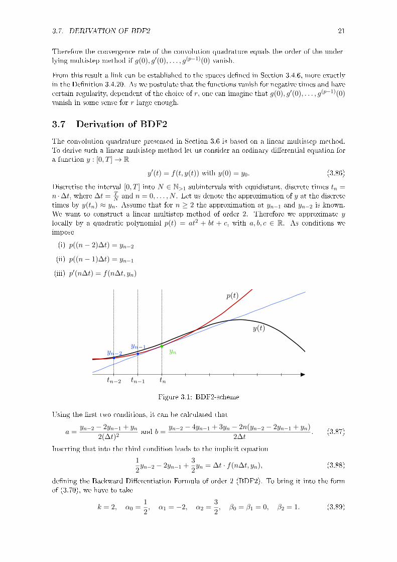
The convolution quadrature presented in Section 3.6 is based on a linear multistep method.To derive such a linear multistep method let us consider an ordinary dierential equation fora function y : [0, T ]→ R
y′(t) = f(t, y(t)) with y(0) = y0. (3.86)
Discretise the interval [0, T ] into N ∈ N>1 subintervals with equidistant, discrete times tn =n ·∆t, where ∆t = T
N and n = 0, . . . , N . Let us denote the approximation of y at the discretetimes by y(tn) ≈ yn. Assume that for n ≥ 2 the approximation at yn−1 and yn−2 is known.We want to construct a linear multistep method of order 2. Therefore we approximate ylocally by a quadratic polynomial p(t) = at2 + bt + c, with a, b, c ∈ R. As conditions weimpose
(i) p((n− 2)∆t) = yn−2
(ii) p((n− 1)∆t) = yn−1
(iii) p′(n∆t) = f(n∆t, yn)
tn−2 tn−1 tn
y(t)
p(t)
yn−2
yn−1yn
Figure 3.1: BDF2-scheme
Using the rst two conditions, it can be calculated that
a =yn−2 − 2yn−1 + yn
2(∆t)2and b =
yn−2 − 4yn−1 + 3yn − 2n(yn−2 − 2yn−1 + yn)
2∆t. (3.87)
Inserting that into the third condition leads to the implicit equation
1
2yn−2 − 2yn−1 +
3
2yn = ∆t · f(n∆t, yn), (3.88)
dening the Backward Dierentiation Formula of order 2 (BDF2). To bring it into the formof (3.70), we have to take
k = 2, α0 =1
2, α1 = −2, α2 =
3
2, β0 = β1 = 0, β2 = 1. (3.89)
22 CHAPTER 3. MATHEMATICAL FRAMEWORK
Hence the ratio of the generating polynomials is given by
γ(ζ) =1
2ζ2 − 2ζ +
3
2(3.90)
Proposition 3.7.1. BDF2 is an A-stable linear multistep method of order 2. Furthermore γhas no poles on the unit circle, with the exception of ζ = 1.
For a proof we refer to [HW91, Chapter 5]. The condition for γ is easy to check, as γ is apolynomial. Furthermore the order of an A-stable linear multistep method cannot exceed theorder 2, as it is shown in [ibid.]. Therefore BDF2 is an optimal choice for a linear multistepmethod fullling Proposition 3.7.1.
3.8 Spherical Harmonics
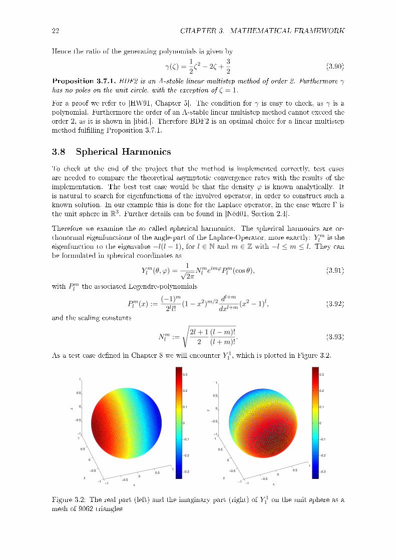
To check at the end of the project that the method is implemented correctly, test casesare needed to compare the theoretical asymptotic convergence rates with the results of theimplementation. The best test case would be that the density ϕ is known analytically. Itis natural to search for eigenfunctions of the involved operator, in order to construct such aknown solution. In our example this is done for the Laplace operator, in the case where Γ isthe unit sphere in R3. Further details can be found in [Néd01, Section 2.4].
Therefore we examine the so called spherical harmonics. The spherical harmonics are or-thonormal eigenfunctions of the angle-part of the Laplace-Operator, more exactly: Y m
l is theeigenfunction to the eigenvalue −l(l − 1), for l ∈ N and m ∈ Z with −l ≤ m ≤ l. They canbe formulated in spherical coordinates as
Y ml (θ, ϕ) =
1√2πNml e
imϕPml (cos θ), (3.91)
with Pml the associated Legendre-polynomials
Pml (x) :=(−1)m
2ll!(1− x2)m/2
dl+m
dxl+m(x2 − 1)l, (3.92)
and the scaling constants
Nml :=
√2l + 1
2
(l −m)!
(l +m)!. (3.93)
As a test case dened in Chapter 8 we will encounter Y 11 , which is plotted in Figure 3.2.
−1−0.5
00.5
1
−1
−0.5
0
0.5
1
−1
−0.5
0
0.5
1
x
y
z
−0.3
−0.2
−0.1
0
0.1
0.2
0.3
−1
−0.5
0
0.5
1
−1
−0.5
0
0.5
1
−1
−0.5
0
0.5
1
x
y
z
−0.3
−0.2
−0.1
0
0.1
0.2
0.3
Figure 3.2: The real part (left) and the imaginary part (right) of Y 11 on the unit sphere as a
mesh of 9062 triangles

Chapter 4
Theory for the Exact Problem
The wave equation (2.4a) encountered in the formulation of the problem (cf. Chapter 2)is called the scalar acoustic wave equation. Before starting to investigate the existence anduniqueness of solutions, some fundamental properties of that equation are listed in the nextsection. This includes the physical background as well as some mathematical properties.
4.1 Properties of the Wave Equation
The scalar acoustic equation describes the propagation of an acoustic wave in a homogeneousmedium. The wave is described by the dierence of the pressure u with respect to the formerresting state, where the pressure was in an equilibrium. Dierent media have dierent speedof sound c > 0. The scalar acoustic equation in its general form depends on the speed ofsound c and is given by
1
c2utt −∆u = 0. (4.1)
However, the function u(x, t) := u(x, c · t) solves the scalar acoustic equation utt − ∆u =0. Therefore, throughout this paper it is supposed that c = 1, as by a scaling of variablesolutions for other arising speeds of sound can be obtained. The nite velocity of the wave isa fundamental property assigned to solutions of the wave equation. If u at a certain time isjust non-zero inside a bounded domain, i.e. u has compact support, then u will have compactsupport at any time, as every disturbance propagates just with the nite velocity c.
Furthermore, as we solve the wave equation in the three dimensional space R3, the wavesare propagating according to the Huygens-Fresnel principle. This states that every point ofa wave at a certain time is the origin of a new spherical wave, which will propagate startingat this time. A whole wave then is the superposition of all these spherical waves started at acertain point. In this context the notion of retarded time arises. Let us x a point x ∈ R3 anda time t > 0. The goal is now to determine all possible origins and starting times of sphericalwaves that reach x at the time t. Assuming y ∈ R3 is another point, then a spherical wavehas an inuence on the pressure at the point x and time t if and only if it has started at y atthe time τ = t− ‖x−y‖c , as exactly in that time, the spherical wave with velocity c has reachedx. Furthermore the disturbance at x has to be smaller than the disturbance at the startingtime in y, as the energy
E(t) =
∫Ω|ut(x, t)|2 + ‖∇u(x, t)‖2dx, (4.2)
is constant for the original problem Porig, supposing nite energy at the starting point t = 0.This follows from dE
dt = 0, which can be shown by using Green's formulas, the wave equationand the imposed Dirichlet condition. This physical considerations are recognized in the formof the fundamental solution k (cf. (2.6)).
23
24 CHAPTER 4. THEORY FOR THE EXACT PROBLEM
4.2 Existence and Uniqueness for the full space Problem
During the process of reducing our original problem Porig to a homogeneous equation the fullspace problem Pinc arises as presented in Chapter 2. It is the Cauchy problem for the waveequation in the form of
∂2t u(x, t)−∆u(x, t) = f(x, t) in R3 × (0, T ) (4.3a)
u(x, 0) = u0(x) ∀x ∈ R3 (4.3b)
∂tu(x, 0) = u1(x) ∀x ∈ R3. (4.3c)
The theory to solve this problem is developed in [Wla72, pp. 161-165], where the classical aswell as the weak solution can be found. We mention here just the classical solution in thethree dimensional case, as it is well illustrating the inuence of the given data on the solutionu.
Theorem 4.2.1. Assume f ∈ C2(R3× [0,∞)), u0 ∈ C3(R3), u1 ∈ C2(R3). Then the classical
solution of the Cauchy problem of the wave equation exists, is unique and is described by the
Kirchho Formula
u(x, t) =
∫Bt(x)
f(y, t− ‖x− y‖)4π‖x− y‖
dy +1
4πt
∫∂Bt(x)
u1(y)dSy +1
4π
∂
∂t
(1
t
∫∂Bt(x)
u0(y)dSy
)(4.4)
Examining this result in more details would show that this formula matches the physicalconsiderations done in Section 4.1. Hence, to prove the existence and uniqueness of thesolution for the original problem Porig, the homogeneous exterior problem Pinc still has to besolved. The existence and uniqueness of such a solution is stated in Section 4.7 using a singlelayer potential representation.
4.3 Motivation for the Single Layer Potential
As noted the Chapter 2, we want to nd a solution u in the form of a single layer potential
u(x, t) =
∫ t
0
∫Γk(x− y, t− τ)ϕ(y, τ)dΓydτ ∀(x, t) ∈ Ω× [0, T ]. (4.5)
In [HD03, Section 2.1] a result of classical electromagnetical scattering theory is presented.Let u be a solution of the homogeneous wave equation with arbitrary boundary conditionsand vanishing initial conditions on R3 \ Γ, i.e. ue resp. ui solves the problem on Ωe × (0, T )resp. Ωi × (0, T ) and u|Ωe = ue resp. u|Ωi = ui. Let us dene the jump of u and its normalderivative
[γ0u](x, t) := ue(x, t)− ui(x, t), [γ1u](x, t) :=∂ue∂ν
(x, t)− ∂ui∂ν
(x, t) (x, t) ∈ Γ× (0, T ),
(4.6)
where ν is the outer normal vector on Γ. Then the solution u has the following integralrepresentation
u(x, t) =
∫Γ
ν(y) · (x− y)
4π‖x− y‖
([γ0u](y, s)
‖x− y‖2+
∂[γ0u]∂t (y, s)
‖x− y‖
)dΓy
−∫
Γ
[γ1u](y, s)
4π‖x− y‖dΓy, (4.7)

4.4. CONNECTION TO THE HELMHOLTZ EQUATION 25
with the retarded time s = t−‖x− y‖. Under the assumption that we are solving a Dirichletproblem with the same boundary condition for the interior and exterior problem. If a contin-uous solution exists for both problems the jump of the function u over the boundary vanishes,i.e. [γ0u] = 0. Hence, the rst integral term in the representation (4.7) disappears and itholds
u(x, t) =
∫Γ
−[γ1u](y, s)
4π‖x− y‖dΓy. (4.8)
Thus, it makes sense to apply a single layer potential in order to solve a Dirichlet problem.
4.4 Connection to the Helmholtz Equation
As a rst try to solve the wave equation, one could try the separation of time and spacevariable, i.e. u(x, t) = X(x)T (t). Furthermore, assume that u is harmonic in time. Therefore,T is of the form T (t) = eiκt for a real κ. Applying the wave equation to such a u leads to
(∂tt −∆)u(x, t) = −κ2X(x)T (t)−∆X(x)T (t) = 0. (4.9)
As T is known one gets an equation for X by dividing formally by T (t)
−κ2X(x)−∆X(x) = 0. (4.10)
This is the homogenous Helmholtz equation.
For a general solution u of the wave equation given by (2.4) the Laplace transform is applied.Therefore, let u be a solution of the exterior Dirichlet problem P and assume that u is Laplacetransformable for Re (s) > σ with respect of t for a σ > 0. The aim is to derive a partialdierential equation, that the Laplace transform u satises. Hence, let us apply the Laplacetransform on (2.4a). For s ∈ C with Re (s) > σ it holds∫ ∞
0e−st(utt(x, t)−∆u(x, t))dt =
∫ ∞0
e−stutt(x, t)dt−∆
∫ ∞0
e−stu(x, t)dt︸ ︷︷ ︸u(x,s)
. (4.11)
The rst term has to be considered furthermore. Using partial integration leads to∫ ∞0
e−stutt(x, t)dt =ut(x, t) · e−st∣∣∞0
+ s
∫ ∞0
e−stut(x, t)dt = ut(x, 0) + s
∫ ∞0
e−stut(x, t)dt
(4.12)
=ut(x, 0) + s(u(x, t) · e−st
)∣∣∞0
+ s2
∫ ∞0
e−stu(x, t)dt (4.13)
=ut(x, 0) + su(x, 0) + s2u(x, s) = s2u(x, s), (4.14)
where in the last step the zero initial conditions (2.4b) and (2.4c) were used. For the boundarycondition (2.4d) weget
u(x, s) = g(x, s), x ∈ Γ, (4.15)
under the assumption that g is Laplace transformable. Hence, the partial dierential equationfor u is given by
−∆u(·, s) + s2u(·, s) = 0 in Ω (4.16a)
u(·, s) = g(·, s) on Γ. (4.16b)

26 CHAPTER 4. THEORY FOR THE EXACT PROBLEM
To bring that equation into the form, in which a Helmholtz problem is usually stated (cf.(4.10)), one substitutes κ = is. Dropping the second argument, as it is just a parameter,leads to the Helmholtz equation for u
−∆u− κ2u = 0 in Ω (4.17)
u = g on Γ. (4.18)
This is the motivation to look at the Helmholtz equation in more detail.
4.5 Theory for the Helmholtz Problem
The theory about the Helmholtz problem is developed in [Néd01] and [SS04]. The problemto solve is dened by
−∆u− κ2u = 0 on Ωe (4.19a)
u = g on Γ (4.19b)
|u(x)| ≤ C1‖x‖−1 for ‖x‖ 7→ ∞ (4.19c)∣∣∣∣∂u∂r − iκu∣∣∣∣ ≤ C2‖x‖−2 for ‖x‖ 7→ ∞, (4.19d)
for given boundary data g, wave number κ ∈ C, r = x‖x‖ and Ωe ⊂ R3 an exterior unbounded
domain. The two conditions (4.19c) and (4.19d) assure the uniqueness of the solution. (4.19c)guarantees the decay towards innity and (4.19d) is called Sommerfeld radiation condition.It assures that only outgoing waves are considered as solutions i.e. no new waves arise fromthe boundary at innity. To solve the problem (4.19), a weighted Sobolev space is introducedfor incorporating the radiation conditions into the space, where the function is searched. Letus introduce the dierential operator Lκ := −∆− κ2. One denes the scalar product
(u, v)H1(Lκ,Ωe) :=
∫Ωe
〈`u,
`v〉+ uv
1 + ‖x‖2+
(∂u
∂r− iκu
)(∂v
∂r− iκv
)dx. (4.20)
The space H1(Lκ,Ωe) is dened as the completion of C∞c (Ωe) := ϕ|Ωe | ϕ ∈ C∞0 (R3) with
respect to the norm ‖·‖H1(Lκ,Ωe):=√
(·, ·)H1(Lκ,Ωe). The existence and uniqueness can then
be found in [Néd01, Theorem 2.6.6], which are proved using the Lemma of Lax-Milgram.
Theorem 4.5.1. If g ∈ H1/2(Γ) then the variational formulation of (4.19) admits a unique
solution in the space H1(Lκ,Ωe). The associated mapping is continuous from H1/2(Γ) into
H1(Lκ,Ωe).
The proof is based on the fact that the single layer potential operator of the Helmholtz problemdiers only in a compact perturbation in comparison to the one of the Laplace problem, whichis elliptic.
An interesting remark is that the exterior problem (4.19), in contrary to the interior problem,that is given by replacing Ωe by Ωi in (4.19), has a solution for every κ, whereas the interiorproblem only has a solution if and only if κ2 is not an eigenvalue of the interior problem forthe Laplace equation. Unfortunately this problem arises if one wants to solve the exteriorproblem (4.19) using the single layer potential. The related theory can be found in [SS04,Chapter 3.9]. We just want to recall the most important points concerning the application ofa single layer potential ansatz for the Helmholtz problem. The fundamental solution of theHelmholtz equation is given by
Gκ(x) =eiκ‖x‖
4π‖x‖. (4.21)
4.5. THEORY FOR THE HELMHOLTZ PROBLEM 27
An important remark is the connection to the Laplace transformed fundamental solution ofthe wave equation k (cf. (3.21)). Applying once more the substitution κ = is one gets thelink
Gκ(x) = k(‖x‖,−iκ). (4.22)
The single layer potential for the Helmholtz equation is dened as (further details are givenin Section 3.5)
(Sϕ)(x) :=
∫ΓGκ(x− y)ϕ(y)dΓy, x ∈ Ωe. (4.23)
As well as for the wave equation, there is a result motivating that choice. In [SS04] the rep-resentation of the solution of elliptic partial dierential equation using Green's third identityis deduced. [SS04, Theorem 3.1.13] just gives the representation
Theorem 4.5.2. Consider the Helmholtz operator Lκu := −∆u−κ2u in the three dimensional
space for a wavenumber κ > 0. If u ∈ H1(Ωi)×H1(Lκ,Ωe) solves Lκu = 0 in R3 \ Γ, then it
holds
u = −S[γ1u] +D[γ0u], (4.24)
with S the single layer operator and D the double layer operator1 for the Helmholtz problem.
Using the same arguments as for the wave equation developed in Section 4.7 we get themotivation for solving the Dirichlet problem of the Helmholtz problem using a single layerpotential.
Altough the exterior Dirichlet problem for the Helmholtz equation admits a unique solutionfor each κ ∈ C, there arise problems by applying the approach of a single layer potential. Themain result is given by [SS04, Theorem 3.9.1] and states that there are critical values for κ,for which the single layer potential operator is not invertible.
Theorem 4.5.3. The single layer potential operator of the Helmholtz problem for a κ ∈ C is
invertible on H−1/2(Γ) if and only if κ2 is not an eigenvalue of the interior problem of the
Laplace equation.
Therefore, if one wants to solve an exterior Helmholtz problem using the single layer potential,one has to assure that κ2 is not an eigenvalue of the interior Laplace problem. Therefore it isimportant to know more about these critical values. The Laplace operator −∆ is a symmetricelliptic operator. The following result for the eigenvalues of such operators can be found in[Eva98, Theorem 1, p. 335].
Theorem 4.5.4. All eigenvalues of a symmetric elliptic operator are real and positive.
Hence, a sucient condition on the arising κ is useful, to avoid the problem of the non-invertibility of the single layer potential operator. A condition that will match the wavenumbers used in this thesis is presented in the following Proposition.
Proposition 4.5.5. A wave number κ ∈ C with Im (κ) > 0 is not a critical value and allows
therefore to employ the single layer potential given by (4.23) in order to solve the exterior
Dirichlet problem of the Helmholtz equation as dened in (4.19).
Proof. Let be κ = a + bi with a, b ∈ R and b > 0. It holds for the squared wave numberκ2 = a2 − b2 + 2abi. Assume, that κ2 is real, i.e. 2ab = 0. As b > 0, it follows that a = 0,which results in κ2 = −b2 < 0. Therefore, no critical value can occur for such κ.
1For the denition and the properties of the double layer operator D we refer to [SS04, Section 3.1].
28 CHAPTER 4. THEORY FOR THE EXACT PROBLEM
4.6 Properties of the Single Layer Potential
First of all, the single layer potential as noted in (2.5) has a distributional kernel k. It isgiven by the fundamental solution of the wave equation. A detailed derivation of it is omittedto [Wla72, Chapter 10]. Its derivation relies on the theory of distributions, the generalizedfunctions. The fundamental solution has to satisfy
ktt(x, t)−∆k(x, t) = δ(x)δ(t) ∀ (x, t) ∈ R3 × R>0 (4.25a)
k(x, t) = 0 ∀ (x, t) ∈ R3 × R≤0, (4.25b)
where the occuring derivatives are derivatives in the sense of distributions and δ the Diracdistribution. By applying the Fourier transform on the rst equation with respect to thevariable x, an ordinary dierential equation in t arises, which can be solved explicitly. Theresult then is transformed back by the inversion formula for the Fourier transform.
Before starting examining the single layer potential, let us try to get rid of the distributionalterm in k. Hence
(Sϕ)(x, t) =
∫ t
0
∫Γk(x− y, t− τ)ϕ(y, τ)dΓydτ =
∫ t
0
∫Γ
δ(‖x− y‖ − (t− τ))
4π‖x− y‖ϕ(y, τ)dΓydτ.
(4.26)
Furthermore it holds τ ≤ t and therefore
‖x− y‖ − (t− τ) = 0 ⇐⇒ τ = t− ‖x− y‖, (4.27)
i.e. exactly in the case when τ is equal to the retarded time t− ‖x− y‖. Formally changingthe order of integration and setting ϕ(·, s) = 0 for s < 0, leads to
(Sϕ)(x, t) =
∫Γ
∫ t
0k(x− y, t− τ)ϕ(y, τ)dτdΓy =
∫Γ
ϕ(y, t− ‖x− y‖)4π‖x− y‖
dΓy, (4.28)
that is the representation deduced in Section 4.3 (cf. equation (4.8)).
Let us continue with the theorems about the properties and regularity of the single layerpotential. First it will be shown that the single layer potential satises the wave equation andthe initial values conditions.
Theorem 4.6.1. For x ∈ Ωe, ϕ regular enough and vanishing for t < 0, the single layer
potential (Sϕ)(x, t) solves the wave equation
utt(x, t)−∆u(x, t) = 0 in Ωe × (0, T ) (4.29a)
u(x, 0) = ut(x, 0) = 0 on Ωe, (4.29b)
Proof. Let us dene u(x, t) := (Sϕ)(x, t) on Ωe×(0, T ). Remark that for a xed x ∈ Ωe, thereexists a C > 0, such that ‖x− y‖ ≥ C for every y ∈ Γ. Hence the integral in the denitionof (Sϕ)(x, t) exists as a proper integral, as Γ is supposed to be compact. Therefore theintegration and dierentiation can be interchanged. Using the same argument one can showthe continuity on Ωe. Let us denote by ϕt, ϕtt the derivatives of ϕ in the second argument.Furthermore it holds for x 6= y
∂
∂xi‖x− y‖ =
∂
∂xi
√(x1 − y1)2 + (x2 − y2)2 + (x3 − y3)2 =
xi − yi‖x− y‖
∀i ∈ 1, 2, 3. (4.30)

4.6. PROPERTIES OF THE SINGLE LAYER POTENTIAL 29
Let us calculate now the derivatives in the time variable of u using the representation (4.28)
ut(x, y) =
∫Γ
ϕt(y, t− ‖x− y‖)4π‖x− y‖
dΓy, (4.31)
utt(x, y) =
∫Γ
ϕtt(y, t− ‖x− y‖)4π‖x− y‖
dΓy. (4.32)
The next step is to determine the derivatives in space using the same representation
uxi =
∫Γ−ϕ(y, t− ‖x− y‖)
4π‖x− y‖2· xi − yi‖x− y‖
− ϕt(y, t− ‖x− y‖)4π‖x− y‖
· xi − yi‖x− y‖
dΓy (4.33)
= −∫
Γϕ(y, t− ‖x− y‖) · xi − yi
4π‖x− y‖3+ ϕt(y, t− ‖x− y‖) ·
xi − yi4π‖x− y‖2
dΓy, (4.34)
uxixi = −∫
Γ−(xi − yi)2
‖x− y‖· ϕt(y, t− ‖x− y‖)
4π‖x− y‖3+ϕ(y, t− ‖x− y‖)
4π‖x− y‖3
− (xi − yi)2
‖x− y‖· 3ϕ(y, t− ‖x− y‖)
4π‖x− y‖4− (xi − yi)2
‖x− y‖· ϕtt(y, t− ‖x− y‖)
4π‖x− y‖2
+ϕt(y, t− ‖x− y‖)
4π‖x− y‖2− (xi − yi)2
‖x− y‖· 2ϕt(y, t− ‖x− y‖)
4π‖x− y‖3dΓy. (4.35)
The last step is to sum now over i. Using
3∑i=1
(xi − yi)2
‖x− y‖= ‖x− y‖, (4.36)
leads to
−∆u =
∫Γ−ϕt(y, t− ‖x− y‖)
4π‖x− y‖2+ 3
ϕ(y, t− ‖x− y‖)4π‖x− y‖3
− 3ϕ(y, t− ‖x− y‖)
4π‖x− y‖3
− ϕtt(y, t− ‖x− y‖)4π‖x− y‖
+ 3ϕt(y, t− ‖x− y‖)
4π‖x− y‖2− 2
ϕt(y, t− ‖x− y‖)4π‖x− y‖2
dΓy (4.37)
= −∫
Γ
ϕtt(y, t− ‖x− y‖)4π‖x− y‖
dΓy. (4.38)
Finally that shows that u satises
utt −∆u =
∫Γ
ϕtt(y, t− ‖x− y‖)4π‖x− y‖
dΓy −∫
Γ
ϕtt(y, t− ‖x− y‖)4π‖x− y‖
dΓy = 0. (4.39)
Hence we have to look at the values of u and ut for t = 0. For the value of u at t = 0 it holds
u(x, 0) =
∫Γ
ϕ(y,−‖x− y‖)4π‖x− y‖
dΓy. (4.40)
As ‖x− y‖ > 0 and ϕ is vanishing for t < 0, it holds u(x, 0) = 0 for x ∈ Ω. Assuming thatϕ is twice continuously dierentiable with respect to the time variable yields to ϕt = 0 fort < 0. Using the same argument as before ensures ut(x, 0) = 0 as
ut(x, 0) =
∫Γ
ϕt(y,−‖x− y‖)4π‖x− y‖
dΓy. (4.41)
30 CHAPTER 4. THEORY FOR THE EXACT PROBLEM
To impose Dirichlet boundary data, the behaviour of the single layer potential over the bound-ary Γ has to be determined. As discussed in Footnote 2 on Page 17 the representation of thesingle layer potential given by (2.5) holds only for densities ϕ which are regular enough. Toget a representation of S on the boundary Γ, denoted by V , one also has to restrict to regularϕ. As later on all densities ϕ used for the discretisation in space satisfy ϕ(·, t) ∈ S, where Sthe boundary element space is dened as S−1,0 or S0,1, which both are a subset of L∞(Γ) (cf.Section 5.2), we develop a representation of V for ϕ(·, t) ∈ L∞(Γ).
The appropriate spaces with respect to the time are introduced in Section 3.4.6. Theseconsiderations motivate the choice ϕ ∈ C(0, T ;L∞(Γ)).
Theorem 4.6.2. Let Γ be the surface of a bounded Lipschitz domain Ωi ⊂ R3 and ϕ ∈C(0, T ;L∞(Γ)). The integral representing the single layer potential for such a ϕ given by
(Sϕ)(x, t) =
∫Γ
ϕ(y, t− ‖x− y‖)4π‖x− y‖
dΓy, (4.42)
exists as an improper integral for all x ∈ R3 and denes a continuous function Sϕ on R3.
Proof. The proof is based on the proof for the continuity of the single layer potential forthe Laplace equation eected in [Néd01, Theorem 3.1.2]. For arguments t − ‖x− y‖ < 0 setthe value of ϕ to zero. Using the denition of the function space, we get the existence of aconstant M > 0, such that
‖ϕ‖C(0,T ;L∞(Γ)) = supt∈[0,T ]
‖ϕ(·, t)‖L∞(Γ) = supt∈[0,T ]
ess supx∈Γ
|ϕ(x, t)| < M. (4.43)
Therefore, we get a majorant function for the integrand almost everywhere∣∣∣∣ϕ(y, t− ‖x− y‖)4π‖x− y‖
∣∣∣∣ ≤M · 1
4π‖x− y‖∀t ∈ [0, T ], x, y ∈ Γ with x 6= y. (4.44)
Hence the proof is lead back to the case of the single layer potential of the Laplace equationas 1
4π‖x‖ is the fundamental solution of the Laplace equation on R3. First of all we show theexistence as improper integral using a majorant function f that is integrable. To show thatthe integral is transformed onto a two dimensional domain by using the Lipschitz property ofthe domain. The mentioned majorant function f also plays the key role in the proof for thecontinuity, as it allows to interchange the limit, linked to a sequence (xn)n∈N converging tox, and the integration using the theorem of Lebesgue.
4.7 Existence and Uniqueness for the Single Layer Potential
As a last step in the theory of the exact problem, the existence and uniqueness of the problem(2.8) in the formulation using the single layer potential has to be discussed. The results aretaken from [BHD86, Proposition 3] respectively [Lub94, (2.22),(2.24)] and use the functionsspaces dened in Section 3.4.6.
Theorem 4.7.1. Let g ∈ Hr+20 (0, T ;H1/2(Γ)) for some r ∈ R. Then
(V ϕ)(x, t) :=
∫ t
0
∫Γk(x− y, t− τ)ϕ(y, τ)dΓydτ = g(x, t) ∀ (x, t) ∈ Γ× (0, T ), (4.45)
has an unique solution ϕ ∈ Hr0(0, T ;H−1/2(Γ)) with
‖ϕ‖Hr0 (0,T ;H−1/2(Γ)) ≤ CT ‖g‖Hr+2
0 (0,T ;H1/2(Γ)). (4.46)
4.7. EXISTENCE AND UNIQUENESS FOR THE SINGLE LAYER POTENTIAL 31
For r > 1/2, the pointwise estimate
‖ϕ(·, t)‖H−1/2(Γ) ≤ CT ‖g‖Hr+20 (0,T ;H1/2(Γ)), (4.47)
holds for all t ∈ [0, T ].
Proof. The proof can be found in [Lub94]. The most important steps and ideas are listed inthis sketch of the proof. Fundamental is the reducing of the wave equation to the Helmholtzequation using the Laplace transform. That also holds for the single layer potential by settingϕ(y, τ) = 0 for τ < 0 and keeping in mind that for τ > t holds ‖x− y‖ − (t− τ) > 0.
L(V ϕ)(s) = L(∫ t
0
∫Γ
δ(‖x− y‖ − (t− τ))
4π‖x− y‖ϕ(y, τ)dΓydτ
)(s) (4.48)
= L(∫ t
−∞
∫Γ
δ(‖x− y‖ − (t− τ))
4π‖x− y‖ϕ(y, τ)dΓydτ
)(s) (4.49)
= L(∫ ∞∞
∫Γ
δ(‖x− y‖ − (t− τ))
4π‖x− y‖ϕ(y, τ)dΓydτ
)(s) (4.50)
= L(∫
Γk(‖x− y‖, t) ∗ ϕ(y, t)dΓy
)(s) (4.51)
=
∫ΓL(k(‖x− y‖, t) ∗ ϕ(y, t))(s)dΓy (4.52)
=
∫Γk(‖x− y‖, s)ϕ(y, s)dΓy =: V(s)ϕ(·, s), (4.53)
with k as in the Section 3.3 being the fundamental solution of the Helmholtz problem as wehave seen in the Section 4.5. Hence the existence and uniqueness of the single layer potentialfor the Helmholtz problem, denoted by V(s), can be considered. As this is discussed inChapter 4.5 with all necessary references, only the results needed for the transformation backto the wave equation are quoted here. It is provided by [BHD86] and is cited in [Lub94,Proposition 2.3].
Lemma 4.7.2. For Re (s) = σ > 0, the single layer potential operator for the Helmholtz
problem V(s) extends by density to an isomorphism
V(s) : H−1/2(Γ)→ H1/2(Γ), (4.54)
which for all ψ ∈ H−1/2(Γ) satises coercivity and boundedness
Re (〈sV(s)ψ,ψ〉) ≥ c · min(1, σ)
|s|‖ψ‖2H−1/2(Γ) (4.55)
‖V(s)ψ‖ ≤ C · |s| · max(1, σ−2)
σ‖ψ‖H−1/2(Γ), (4.56)
where c and C are positive constants, which depend only on Γ.
Therefore, we get the following mapping property for the single layer potential
V(s) : H−1/2(Γ)→ H1/2(Γ), ϕ 7→ g (4.57)
where ϕ is the density and g the Dirichlet data. Furthermore a bound for V−1(s) is neededand is provided by [BHD86, Proposition 2] and quoted in [Lub94, Equation 2.20].
Lemma 4.7.3. For Re (s) > σ0 > 0 the following bound holds∥∥V−1(s)∥∥ ≤M(σ0) · |s|2, (4.58)
where M(σ0) is a positive constant depending on σ0 and Γ.
32 CHAPTER 4. THEORY FOR THE EXACT PROBLEM
The transform of this estimate to the wave equation in the time domain is presented in[Lub94]. In the 'operational calculus' the convolution with respect to the time of the formk ∗ g is denoted by k(∂t)g to emphasize on Laplace transform k of k instead of k itself.Furthermore, using only k, k(∂t)g is given by the following Denition.
Denition 4.7.4. Let k(s) be an analytic function for Re (s) > σ0 that is bounded for large
|s| by ∣∣∣k(s)∣∣∣ ≤M · |s|µ, (4.59)
for µ ∈ R. Let σ > σ0, N 3 m > µ+ 1 and g ∈ Cm(R). Then k(∂t)g is dened by
(k(∂t)g
)(t) :=
∫ ∞0
(1
2πi
∫σ+iR
esτk(s)
smds
)g(m)(t− τ)dτ. (4.60)
The properties of the operator k(∂t) include the composition rule
k2(∂t)k1(∂t)g =(k2 · k1
)(∂t)g (4.61)
and, for g Laplace transformable, the relation
L(k(∂t)g
)(s) = k(s) · (Lg)(s) (4.62)
on the appropriate half-plane in C. The essence of this approach is summarized in the followingTheorem.
Theorem 4.7.5. If k(s) is an analytic function for Re (s) > σ0 that is bounded for large |s|by ∣∣∣k(s)
∣∣∣ ≤M · |s|µ, (4.63)
for µ ∈ R, then k(∂t) and therefore k ∗ g extends by density to a bounded linear operator
k(∂t) : Hr+µ0 (0, T )→ Hr
0(0, T ). (4.64)
This theory is applied to Banach space valued operators. Using the denition of the integraloperator
z(t) : H−1/2(Γ)→ H1/2(Γ), f 7→∫
Γ
δ(‖· − y‖ − t)4π‖· − y‖
f(y)dΓy, (4.65)
the equation (4.45) can be rewritten in terms of time convolution of integral operators on Γ∫ t
0
∫Γ
δ(‖x− y‖ − (t− τ))
4π‖x− y‖ϕ(y, τ)dΓydτ =
(∫ t
0z(t− τ)ϕ(·, τ)dτ
)(x) (4.66)
=
(∫ ∞−∞
z(t− τ)ϕ(·, τ)dτ
)(x) = ((z ∗ ϕ)(t))(x) = g(x, t), on Γ× [0, T ], (4.67)
or as equation in H1/2(Γ)
(z ∗ ϕ)(t) = g(·, t), t ∈ [0, T ]. (4.68)
Applying the Laplace transform on the left-hand side of (4.68), we get
L(z ∗ ϕ)(s) = z(s)ϕ(s). (4.69)
4.7. EXISTENCE AND UNIQUENESS FOR THE SINGLE LAYER POTENTIAL 33
Hence, for the Laplace transformed operator z(s) we exactly get the mapping,
f 7→∫
Γ
e−s‖·−y‖
4π‖· − y‖f(y)dΓy, (4.70)
which is the single layer potential operator for the Helmholtz problem z(s) = V(s). Thereforeusing the calculus mentioned above one can write the equation (4.45) as
V(∂t)ϕ = g. (4.71)
Using the mapping properties of V(s) and the composition rule presented in (4.61), one gets
ϕ(t) = (V−1(∂t)V(∂t)ϕ)(t) = (V−1(∂t)g)(t). (4.72)
Taking the bound of Lemma 4.7.3, the result of Theorem 4.7.5 and the mapping properties intoconsideration, one gets the asserted mapping properties of V . Furthermore the boundednessgiven in the latter theorem leads to the stated estimates. For r > 1/2 Sobolev's embeddingtheorem implies that ϕ ∈ Hr
0(0, T ;H−1/2(Γ)) has a continuous representative with respect tothe time variable. Therefore a pointwise estimate is possible.

34 CHAPTER 4. THEORY FOR THE EXACT PROBLEM

Chapter 5
Numerical Discretisation
In order to calculate the solution of the wave equation given by (2.4), an indirect methodusing the single layer potential is applied. The goal therefore is to determine the unknowndensity ϕ numerically, which will allow the calculation u at any given eld point in the exteriordomain for any given time. Before applying a boundary element method as discretisation inspace, the time dependence is discretized by applying the convolution quadrature presentedin Section 3.6.
5.1 Time Discretisation
The rst step is to discretise (2.8) in the time variable t. Let ∆t = TN be the time step for a
N ∈ N>0. The N + 1 equidistant discrete times are dened by tn = n ·∆t, for n = 0, . . . , N .Recall the integral equation∫ t
0
∫Γk(x− y, t− τ)ϕ(y, τ)dΓydτ = g(x, t) ∀ (x, t) ∈ Γ× (0, T ). (5.1)
In this case, in comparison to the convolution of two real valued functions (cf. Section 3.6),the coecients ω∆t
n depend also on the space variable, i.e. they are functions themselves. As
k(x− y, t− τ) = δ(‖x−y‖−(t−τ))4π‖x−y‖ , they just depend on ‖x− y‖. If the two integrals in (5.1) are
commutable, we get (5.1) in convolution form∫ t
0
∫Γk(x− y, t− τ)ϕ(y, τ)dΓydτ =
∫Γ
∫ t
0k(x− y, t− τ)ϕ(y, τ)dτdΓy (5.2)
≈∫
Γ
n∑j=0
ω∆tn−j(‖x− y‖)ϕ∆t
j (y)dΓy =n∑j=0
∫Γω∆tn−j(‖x− y‖)ϕ∆t
j (y)dΓy.
(5.3)
Therefore, let us dene the discrete convolution operator
(V ϕ)n :=n∑j=0
∫Γω∆tn−j(‖x− y‖)ϕ∆t
j (y)dΓy, n = 0, . . . , N, (5.4)
which leads to the semi-discrete problem
(V ϕ)n(x) = gn(x), n = 1, . . . , N, x ∈ Γ, (5.5)
with gn(x) = g(x, tn).
Using d := ‖x− y‖ the coecients ω∆tn (‖x− y‖) are denoted as functions ω∆t
n (d) with respectto d. The next step is to calculate these coecients using the rule developed in Section 3.6.
35

36 CHAPTER 5. NUMERICAL DISCRETISATION
Due to the considerations in Section 3.7, we use BDF2, an A-stable linear multistep methodof order 2, for the discretisation. The ratio of the corresponding generating polynomials (3.7)is given by
γ(ζ) =1
2ζ2 − 2ζ +
3
2. (5.6)
As explained in Section 3.6 (cf. (3.83)) the coecients of the power series of f(γ(ζ)∆t
)with
respect to ζ are the weights ω∆tn . For the case of k being the fundamental solution of the wave
equation, it is shown in [HKS09] that ω∆tn can be represented explicitly by
ω∆tn (d) =
1
n!
1
4πd
(d
2∆t
)n/2e−
3d2∆tHn
(√2d
∆t
), (5.7)
where Hn denote the n-th Hermite polynomial. There are several possibilities how to calculateω∆tn (d) as discussed in Section 5.3.
5.2 Space Discretisation
To discretise the spatial problem on Γ a Galerkin boundary element method is applied. Firstof all a surface paneling of Γ is needed.
5.2.1 Surface Paneling
The theory, which is presented here, follows [SS04, Chapter 4.1.2]. We introduce a boundaryelement mesh, also called paneling, G on Γ. We restrict to plane triangles with straight edges,i.e. Γ is the surface of a polyhedron. Let τ ∈ G, then we have a parametrization χτ : τ → τ ,where τ is the unit triangle dened by
τ = conv
(00
),
(10
),
(11
). (5.8)
Let us dene for a triangle τ with vertices A,B,C ∈ R3 the matrix Mτ by
Mτ :=
B−A C−B
. (5.9)
Then the parametrization χτ is ane and is dened by
χτ (x) = A + Mτ ·(x1
x2
). (5.10)
The matrix Mτ is the Jacobian of χτ . If τ is not degenerated, i.e. the vertices are notcolinear, the columns of the matrix Mτ are linearly independent and therefore MT
τ Mτ ispositive denite. Thus there exist λmin, λmax > 0 such that
0 < λmin ≤ infv∈R2,‖v‖=1
vTMTτ Mτv ≤ sup
v∈R2,‖v‖=1
vTMTτ Mτv ≤ λmax <∞. (5.11)
Hence the mapping χτ is regular in the sense of [SS04, Denition 4.1.2]. Let us state thedenition for a regular paneling G of Γ.
Denition 5.2.1. A paneling G of the boundary Γ is a partitioning of Γ into relatively open,
disjoint elements τ ⊂ Γ with
5.2. SPACE DISCRETISATION 37
(i) G is a covering of Γ, i.e. Γ =⋃τ∈G τ .
(ii) Each element τ ∈ G is the image of the reference element τ using a regular χτ as stated
in (5.11).
As we have seen before, the mappings for the case of plane triangles with straight edges fullthis denition.
Remark 5.2.2. Our assumptions on G imply that Γ is the surface of a polyhedron. If Γ iscurved, then an additional approximation arises if Γ is approximated by plane triangles orhigher order parametric surface elements. For an error analysis we refer to [SS10].
In order to prove error estimates we have to impose additional properties on G.
Denition 5.2.3. A paneling G of Γ is regular if
(i) The intersection of the closure of two dierent elements τ, t ∈ G either is empty or
contains a common vertex or a common edge.
(ii) The parametrizations of common edges are compatible, i.e. if τ, t ∈ G, with τ 6= t, havea common edge e = τ ∩ t, then it holds
χτ |e = χt γτ,t|e, (5.12)
with e = χ−1τ (e) and γτ,t : τ → τ an ane bijection.
The latter point is fullled in the case of plane triangles with straight lines. Assume that Gis regular, i.e. the properties for the intersection of two panels hold, and only contains planetriangles. To get the properties of the triangulation state
Denition 5.2.4.
(i) The diameter of a triangle τ ∈ G is given by hτ := supx,y∈τ ‖x− y‖.
(ii) The inner width ρτ is dened by the incircle diameter of τ .
(iii) The mesh width hG (shorthand: h) is dened by hG := maxτ∈G hτ .
(iv) The shape-regularity constant κG is given by κG := maxτ∈Ghτρτ.
(v) The constant qG decribes the quasi-uniformity by qG := hGminτ∈G hτ
.
The variable ρτ , κG and qG will not be tracked explicitly in the convergence estimates but arehidden in the generic constant C. They just remind us that the various triangulations shouldnot contain too big dierences in terms of the shape of triangles nor degenerate in terms ofextremely cute angles of panels.
Denition 5.2.5. PG is the set of all vertices of G dened by
PG := P ∈ R3 | ∃ τ ∈ G such that P is a vertex of τ (5.13)
For quantity issues we dene the following cardinalities
Denition 5.2.6.
(i) The number of panels in G is dened by Nτ := |G|
(ii) The number of vertices in G is dened by NP := |PG |
Therefore we will number the panels as τk with 1 ≤ k ≤ Nτ resp. the vertices as Pk with1 ≤ k ≤ NP and it holds
τk | 1 ≤ k ≤ Nτ = G resp. Pk | 1 ≤ k ≤ NP = PG . (5.14)
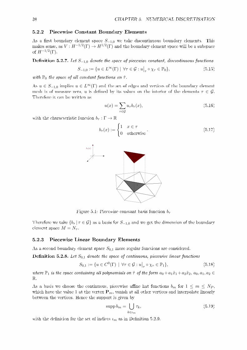
38 CHAPTER 5. NUMERICAL DISCRETISATION
5.2.2 Piecewise Constant Boundary Elements
As a rst boundary element space S−1,0 we take discontinuous boundary elements. Thismakes sense, as V : H−1/2(Γ)→ H1/2(Γ) and the boundary element space will be a subspaceof H−1/2(Γ).
Denition 5.2.7. Let S−1,0 denote the space of piecewise constant, discontinuous functions
S−1,0 := u ∈ L∞(Γ) | ∀τ ∈ G : u∣∣τ χτ ∈ P0, (5.15)
with P0 the space of all constant functions on τ .
As u ∈ S−1,0 implies u ∈ L∞(Γ) and the set of edges and vertices of the boundary elementmesh is of measure zero, u is dened by its values on the interior of the elements τ ∈ G.Therefore it can be written as
u(x) =∑τ∈G
uτ bτ (x), (5.16)
with the characteristic function bτ : Γ→ R
bτ (x) :=
1 x ∈ τ0 otherwise
. (5.17)
τ
bτ (x)
Figure 5.1: Piecewise constant basis function bτ
Therefore we take bτ | τ ∈ G as a basis for S−1,0 and we get the dimension of the boundaryelement space M = Nτ .
5.2.3 Piecewise Linear Boundary Elements
As a second boundary element space S0,1 more regular functions are considered.
Denition 5.2.8. Let S0,1 denote the space of continuous, piecewise linear functions
S0,1 := u ∈ C0(Γ) | ∀τ ∈ G : u∣∣τ χτ ∈ P1, (5.18)
where P1 is the space containing all polynomials on τ of the form a0 +a1x1 +a2x2, a0, a1, a2 ∈R.
As a basis we choose the continuous, piecewise ane hat functions bm for 1 ≤ m ≤ NP ,which have the value 1 at the vertex Pm, vanish at all other vertices and interpolate linearlybetween the vertices. Hence the support is given by
supp bm =⋃k∈ιm
τk, (5.19)
with the denition for the set of indices ιm as in Denition 5.2.9.
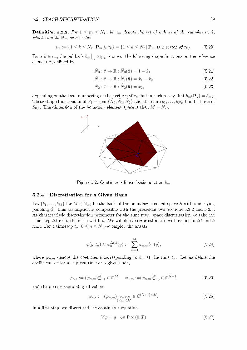
5.2. SPACE DISCRETISATION 39
Denition 5.2.9. For 1 ≤ m ≤ NP , let ιm denote the set of indices of all triangles in G,which contain Pm as a vertex:
ιm := 1 ≤ k ≤ Nτ |Pm ∈ τk = 1 ≤ k ≤ Nτ |Pm is a vertex of τk. (5.20)
For a k ∈ ιm, the pullback bm∣∣τkχτk is one of the following shape functions on the reference
element τ , dened by
N0 : τ → R : N0(x) = 1− x1 (5.21)
N1 : τ → R : N1(x) = x1 − x2 (5.22)
N2 : τ → R : N2(x) = x2, (5.23)
depending on the local numbering of the vertices of τk, but in such a way that bm(Pk) = δmk.These shape functions full P1 = spanN0, N1, N2 and therefore b1, . . . , bNP build a basis ofS0,1. The dimension of the boundary element space is then M = NP .
bm(x)
Pm
Figure 5.2: Continuous linear basis function bm
5.2.4 Discretisation for a Given Basis
Let b1, . . . , bM for M ∈ N>0 be the basis of the boundary element space S with underlyingpaneling G. This assumption is compatible with the precedent two Sections 5.2.2 and 5.2.3.As characteristic discretization parameter for the time resp. space discretisation we take thetime step ∆t resp. the mesh width h. We will derive error estimates with respet to ∆t and hnext. For a timestep tn, 0 ≤ n ≤ N , we employ the ansatz
ϕ(y, tn) ≈ ϕ∆t,hn (y) :=
M∑m=1
ϕn,mbm(y), (5.24)
where ϕn,m denote the coecients corresponding to bm at the time tn. Let us dene thecoecient vector at a given time or a given node,
ϕn,∗ := (ϕn,m)Mm=1 ∈ CM , ϕ∗,m :=(ϕn,m)Nn=0 ∈ CN+1, (5.25)
and the matrix containing all values
ϕ∗,∗ := (ϕn,m) 0≤n≤N1≤m≤M
∈ C(N+1)×M . (5.26)
In a rst step, we discretised the continuous equation
V ϕ = g on Γ× (0, T ) (5.27)

40 CHAPTER 5. NUMERICAL DISCRETISATION
in time and obtained (cf. (5.4))
(V ϕ)n :=n∑j=0
∫Γω∆tn−j(‖x− y‖)ϕ∆t
j (y)dΓy, n = 0, . . . , N. (5.28)
By replacing ϕ∆tj (y) by the ansatz ϕ∆t,h
j (y) results
n∑j=0
∫Γω∆tn−j(‖x− y‖)
M∑m=1
ϕj,mbm(y)dΓy =
n∑j=0
M∑m=1
∫Γω∆tn−j(‖x− y‖)ϕj,mbm(y)dΓy = g(x, tn),
(5.29)
for all x ∈ Γ and 0 ≤ n ≤ N , which is in general an overdetermined system if being consideredpointwise. To obtain a proper formulation (Galerkin discretisation) we impose it in a weakform (cf. Section 3.5). For each time step n we have to determine M coecients. ThereforeM equations have to be obtained and that is made by imposing the weak formulation on Sitself.∫
Γ
n∑j=0
M∑m=1
∫Γω∆tn−j(‖x− y‖)ϕj,mbm(y)dΓy
ψ(x)dΓx =
∫Γg(x, tn)ψ(x)dΓx ∀ψ ∈ S.
(5.30)
As S is the span of the basis functions b1, . . . , bM , it suces to impose (5.30) just for the basisfunctions. Furthermore the outer integration can be interchanged with the two sums, as theyare nite. In general, let g∆t
n (x) equal g(x, tn) or be a suciently accurate approximation toit.
Thus we arrive at the space and time discrete problem using convolution quadrature in timeand a Galerkin discretisation in space
n∑j=0
M∑m=1
ϕj,m
∫Γ
∫Γω∆tn−j(‖x− y‖)bm(y)bk(x)dΓydΓx =
∫Γg∆tn (x)bk(x)dΓx (5.31)
∀ 1 ≤ k ≤M and 0 ≤ n ≤ N.
Dene for each n ∈ 0, . . . , N a right-hand side vector gn ∈ RM and a system matrixAn ∈ RM×M by
(An)k,m :=
∫Γ
∫Γω∆tn (‖x− y‖)bm(y)bk(x)dΓydΓx and (gn)k :=
∫Γg∆tn (x)bk(x)dΓx. (5.32)
The matrices An are fully populated, as their entries are of the form∫
Γ
∫Γ . . . and ω
∆tn is a
non-local function. Furthermore the inner sum and the condition ∀ 1 ≤ k ≤ M of equation(5.31) can be written in vector form resulting in
n∑j=0
An−jϕj,∗ = gn ∀n ∈ 0, . . . , N. (5.33)
This can be written in matrix form leading to a lower Toeplitz system of dimension (N + 1)×(N + 1) with M ×M matrices as block entries. It has the following form
A0 0 · · · 0A1 A0 0
.... . .
. . ....
AN−1 · · · · · · A0 0AN AN−1 · · · A1 A0
ϕ0,∗ϕ1,∗
...
ϕN−1,∗ϕN,∗
=
g0
g1
...
gN−1
gN
. (5.34)
5.3. APPROXIMATION OF THE CONVOLUTION WEIGHTS 41
This is the denition of the linear system for the coecient vector of the solution usingconvolution quadrature in time and a Galerkin discretisation in space. Questions related tothe use of 'Fast Fourier Transform' techniques for its solution resp. numerical quadrature arediscussed in Section 5.3 resp. Section 7.4.
5.3 Approximation of the Convolution Weights
Already in [Lub88b, Section 7] the author listed three possibilities to calculate the convolutionweights, which in fact are functions. In [HKS09] an approximation method is proposed usinga cuto on the representation (5.7) of ω∆t
j (d), where d := ‖x− y‖. In this master thesisthe method proposed in [BS08] is followed. It is based on the approximation of the Cauchyintegral formula by the trapezoidal rule as proposed in [Lub94, equation 3.10]. However in[BS08] this approximation is not just used as approximation: The discrete Fourier transformstyle of the approximation is used to decouple the systems in (5.33). Using this method thesolving of the Toeplitz system (5.34) as in [HKS09] and [HKS07] is avoided.
The coecients ω∆tj (d) are dened as the coecients of the power series of f
(γ(·)∆t
)(cf. Section
3.6, Equation 3.83) . Hence we have to determine the power series of k(d, γ(ζ)
∆t
)with respect
to ζ, where k is the Laplace transform of the fundamental solution of the wave equation k.By using the Cauchy integral formula for higher derivatives, we get for j ∈ N
ω∆tj (d) =
1
2πi
∫|ζ|=λ
k(d, γ(ζ)
∆t
)ζj+1
dζ, (5.35)
for 0 < λ < 1 small enough, such that k(d, γ(ζ)
∆t
)is holomorphic on Bλ+ε(0), for some
suciently small ε > 0. Let us do the approximation using the trapezoidal rule and integratingover the closed curve α : [0, 1]→ C, with α(t) = λe2πit
ω∆tj (d) =
1
2πi
∫α
k(d, γ(ζ)
∆t
)ζj+1
dζ =1
2πi
∫ 1
0
k(d, γ(λe2πit)
∆t
)(λe2πit)j+1
· 2πi · λe2πitdζ (5.36)
=
∫ 1
0k
(d,γ(λe2πit)
∆t
)· λ−je−2πijtdζ (5.37)
≈ λ−j
N + 1
N∑l=0
k
(d,γ(λe
2πilN+1 )
∆t
)e−2πijlN+1 =
λ−j
N + 1
N∑l=0
k
(d,γ(λe
−2πilN+1 )
∆t
)e
2πijlN+1 , (5.38)
where in the last step 0 ≤ l ≤ N is replaced by k = N+1−l. Therefore it holds 1 ≤ k ≤ N+1.
By virtue of e−2πi(N+1)N+1 = 1 = e−
2πi·0N+1 in the case of k = N + 1, we can go back to 0 ≤ k ≤ N
and substituting just the letter k by l.
For the following we introduce some further notation. The quadrature points on the unit
sphere in C are denoted by ζN+1 := e−2πiN+1 . For the second argument in the Laplace transform
k the values κl := iγ(λζlN+1)
∆t are dened, where once more the transformation k = is is used.
Furthermore recall the expression of k
k(d, s) =e−sd
4πd. (5.39)
42 CHAPTER 5. NUMERICAL DISCRETISATION
With these notation at hand we can write
ω∆tj (d) ≈ λ−j
N + 1
N∑l=0
k
(d,γ(λζ lN+1)
∆t
)ζ−ljN+1 =
λ−j
N + 1
N∑l=0
k(d,κli
)ζ−ljN+1 (5.40)
=λ−j
N + 1
N∑l=0
e−κlid
4πdζ−ljN+1 =
λ−j
N + 1
N∑l=0
eiκld
4πdζ−ljN+1. (5.41)
Let us denote by Gκ(·) the fundamental solution of the Helmholtz operator −∆ − κ2 as inSection 4.5, i.e.,
Gκ(d) =eiκd
4πd. (5.42)
With this notation, we nally get the approximation
ω∆tj (d) ≈ λ−j
N + 1
N∑l=0
Gκl(d)ζ−ljN+1. (5.43)
A proposition concerning the quality of that approximation and its compatibility to the dis-cretisation developed in Section 5.2.4 will follow in Section 6.2.
5.4 Decoupling the Systems
Using the results of the last section we are able to rewrite the discrete problem (5.31). Aswe made a further approximation by employing the trapezoidal rule for approximating theCauchy integral, let us denote the coecients by ϕj,m instead of the ϕj,m in the case of theunperturbed discrete problem (5.31), for 0 ≤ j ≤ N , 1 ≤ m ≤M . Let us furthermore extendthe denition of the convolution weights ω∆t
n to negative indices n = −N,−N + 1, . . . ,−1 bysetting ω∆t
n ≡ 0 for such n. Therefore, we can enlarge the rst sum in (5.31) up to N for eachtime step, thus
N∑j=0
M∑m=1
ϕj,m
∫Γ
∫Γω∆tn−j(‖x− y‖)bm(y)bk(x)dΓydΓx =
∫Γg∆tn (x)bk(x)dΓx (5.44)
∀ 1 ≤ k ≤M and 0 ≤ n ≤ N.
Now the convolution weights are replaced by the approximation deduced in the last sectionand transformed coecients ϕl,m :=
∑Nj=0 λ
jϕj,mζljN+1 are introduced.
N∑j=0
M∑m=1
ϕj,m
∫Γ
∫Γ
(λ−(n−j)
N + 1
N∑l=0
Gκl(‖x− y‖)ζ−l(n−j)N+1
)bm(y)bk(x)dΓydΓx (5.45)
=λ−n
N + 1
N∑l=0
M∑m=1
N∑j=0
λjϕj,mζljN+1
∫Γ
∫ΓGκl(‖x− y‖)bm(y)bk(x)dΓydΓx
ζ−lnN+1
(5.46)
=λ−n
N + 1
N∑l=0
M∑m=1
ϕl,m
∫Γ
∫ΓGκl(‖x− y‖)bm(y)bk(x)dΓydΓx
ζ−lnN+1 (5.47)
That leads to the equation
λ−n
N + 1
N∑l=0
M∑m=1
ϕl,m
∫Γ
∫ΓGκl(‖x− y‖)bm(y)bk(x)dΓydΓx
ζ−lnN+1 =
∫Γg∆tn (x)bk(x)dΓx
(5.48)
∀ 1 ≤ k ≤M and 0 ≤ n ≤ N.
5.4. DECOUPLING THE SYSTEMS 43
By looking at the terms one recognizes a scaled discrete Fourier transform as considered inSection 3.1. Let us dene the following terms for k = 1, . . . ,M
al,k :=
M∑m=1
ϕl,m
∫Γ
∫ΓGκl(‖x− y‖)bm(y)bk(x)dΓydΓx, l = 0, . . . , N (5.49)
an,k :=λ−n
N + 1
N∑l=0
M∑m=1
ϕl,m
∫Γ
∫ΓGκl(‖x− y‖)bm(y)bk(x)dΓydΓx
ζ−lnN+1, n = 0, . . . , N.
(5.50)
This denition makes sense as they are coecients of two vectors linked by the scaled discreteFourier transform. Therefore equation (5.48) can be written as
an,k =
∫Γg∆tn (x)bk(x)dΓx ∀ 1 ≤ k ≤M and 0 ≤ n ≤ N. (5.51)
Employing the inverse scaled Fourier transform results in the equivalent equation
al,k =N∑j=0
λjaj,kζljN+1 =
N∑j=0
λj∫
Γg∆tj (x)bk(x)dΓyζ
ljN+1 (5.52)
=
∫Γ
N∑j=0
λjg∆tj (x)ζ ljN+1
bk(x)dΓx ∀ 1 ≤ k ≤M and 0 ≤ l ≤ N. (5.53)
By dening g∆tl (x) :=
∑Nj=0 λ
jg∆tj (x)ζ ljN+1 for 0 ≤ l ≤ N , we get the equations in their nal
form
M∑m=1
ϕl,m
∫Γ
∫ΓGκl(‖x− y‖)bm(y)bk(x)dΓydΓx =
∫Γg∆tl (x)bk(x)dΓx, (5.54)
∀ 1 ≤ k ≤M and 0 ≤ l ≤ N.
Therefore, for each time step 0 ≤ l ≤ N a single Helmholtz problem must be solved. Let usdene the system matrix Al ∈ CM×M and the right-hand side vector gl for 0 ≤ l ≤ N by
(Al)k,m =
∫Γ
∫ΓGκl(‖x− y‖)bm(y)bk(x)dΓydΓx and (gl)k =
∫Γg∆tl (x)bk(x)dΓx. (5.55)
With this notation we get the N + 1 decoupled linear systems for l = 0, . . . , N
Alϕl,∗ = gl, (5.56)
each of which represents a Helmholtz problem with the complex wavenumber κl. By solvingthese systems, a coecient matrix ϕ∗,∗ is deduced. As we are interested in ϕ∗,∗, the obtainedFFT-transformed solution vector has to be transformed back by using the inverse of the scaleddiscrete Fourier transform. Thus for the vector ϕ∗,m it holds
ϕn,m =λ−n
N + 1
N∑l=0
ϕl,mζ−lnN+1 ∀ 0 ≤ n ≤ N and 1 ≤ m ≤M. (5.57)
The last question concerns the wavenumbers κl. As encountered in Section 4.5 there arecritical values for wavenumbers, where the single layer potential is not invertible. As we have
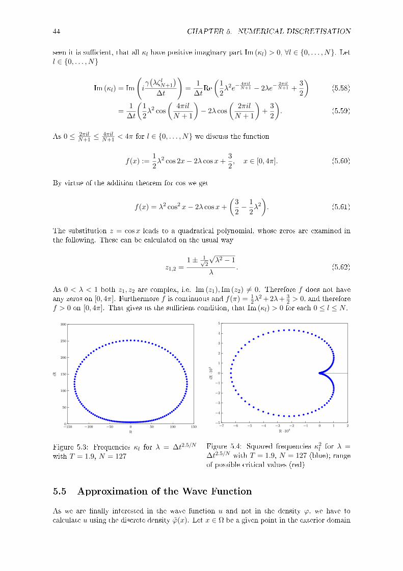
44 CHAPTER 5. NUMERICAL DISCRETISATION
seen it is sucient, that all κl have positive imaginary part Im (κl) > 0, ∀l ∈ 0, . . . , N. Letl ∈ 0, . . . , N
Im (κl) = Im
(iγ(λζ lN+1
)∆t
)=
1
∆tRe
(1
2λ2e−
4πilN+1 − 2λe−
2πilN+1 +
3
2
)(5.58)
=1
∆t
(1
2λ2 cos
(4πil
N + 1
)− 2λ cos
(2πil
N + 1
)+
3
2
). (5.59)
As 0 ≤ 2πilN+1 ≤
4πilN+1 < 4π for l ∈ 0, . . . , N we discuss the function
f(x) :=1
2λ2 cos 2x− 2λ cosx+
3
2, x ∈ [0, 4π]. (5.60)
By virtue of the addition theorem for cos we get
f(x) = λ2 cos2 x− 2λ cosx+
(3
2− 1
2λ2
). (5.61)
The substitution z = cosx leads to a quadratical polynomial, whose zeros are examined inthe following. These can be calculated on the usual way
z1,2 =1± 1√
2
√λ2 − 1
λ. (5.62)
As 0 < λ < 1 both z1, z2 are complex, i.e. Im (z1), Im (z2) 6= 0. Therefore f does not haveany zeros on [0, 4π]. Furthermore f is continuous and f(π) = 1
2λ2 + 2λ+ 3
2 > 0, and thereforef > 0 on [0, 4π]. That gives us the sucient condition, that Im (κl) > 0 for each 0 ≤ l ≤ N .
−150 −100 −50 0 50 100 1500
50
100
150
200
250
300
R
iR
bbbbbbbbbbbbbbbbb
bbbbb
bbbb
bbbbbbbbbbbbbbbbbbbbbbbbbbbbbbbb b b b b b b b b b b b b b b
bbbbbbbbbbbbbbbbbbbbbbbbbbbbbbbbbbbbbbbbbbbbbbbbbbbbbbbb
Figure 5.3: Frequencies κl for λ = ∆t2.5/N
with T = 1.9, N = 127
−7 −6 −5 −4 −3 −2 −1 0 1 2−5
−4
−3
−2
−1
0
1
2
3
4
5
R ·104
iR
·104
b b b b b b b b b b b b b b b b b b b b b b b b b b b bbbbbbbbbbb
bb
bb
bb
bbbbbbbbbb
bb
bb
b
b
b
b
b
b
b
b
b
b
b
b
b
bb
bb
bb b b b b b b b b
bbbbbbbbbbbbbbbbbbbbbbbbbbbbbbbbbbbbbbbbbbb
Figure 5.4: Squared frequencies κ2l for λ =
∆t2.5/N with T = 1.9, N = 127 (blue); rangeof possible critical values (red)
5.5 Approximation of the Wave Function
As we are nally interested in the wave function u and not in the density ϕ, we have tocalculate u using the discrete density ϕ(x). Let x ∈ Ω be a given point in the exterior domain
5.5. APPROXIMATION OF THE WAVE FUNCTION 45
Ω. Using our ansatz we get
u(x, t) =
∫ t
0
∫Γ
δ(‖x− y‖ − (t− τ))
4π‖x− y‖ϕ(y, τ)dΓydτ (5.63)
=
∫Γ
1
4π‖x− y‖ϕ(y, t− ‖x− y‖)dΓy (5.64)
=∑τ∈G
∫τ
1
4π‖x− y‖ϕ(y, t− ‖x− y‖)dΓy. (5.65)
For the time t we use the equidistant discrete times arising in the boundary element methodtl, 0 ≤ l ≤ N . Suppose that bm, 1 ≤ m ≤M is a basis of the approximating space S and ϕn,mare the coecients of the numerical approximation of ϕ, i.e. ϕ(x, tn) =
∑Mm=1 ϕn,mbm(x),
hence
u(x, tl) =∑τ∈G
∫τ
1
4π‖x− y‖ϕ(y, tl − ‖x− y‖)dΓy. (5.66)
As the retarded time t∗ := tl − ‖x− y‖ in general does not coincide with a discrete timepoint, we use a linear interpolation in time to evaluate ϕ at t∗. With n :=
⌊t∗
∆t
⌋, it holds
t∗ ∈ [n∆t, (n + 1)∆t]. Dene t− := n∆t and t+ := (n + 1)∆t. Using linear interpolation weget
ϕ(y, tl − ‖x− y‖) ≈ ϕ(y, t−) + (ϕ(y, t+)− ϕ(y, t−))t∗ − t−
t+ − t−(5.67)
= ϕ(y, t−) + (ϕ(y, t+)− ϕ(y, t−))t∗ − n∆t
∆t(5.68)
= ϕ(y, t−)
(1−
(t∗
∆t− n
))+ ϕ(y, t+)
(t∗
∆t− n
)(5.69)
=M∑m=1
(ϕn,m
(1−
(t∗
∆t− n
))+ ϕn+1,m
(t∗
∆t− n
))· bm(y). (5.70)
Merging these approximations leads to
u(x, tl) ≈M∑m=1
[(ϕn,m
(1−
(t∗
∆t− n
))+ ϕn+1,m
(t∗
∆t− n
))∑τ∈G
∫τ
1
4π‖x− y‖bm(y)dΓy
](5.71)
=
M∑m=1
[(ϕn,m
(1−
(t∗
∆t− n
))+ ϕn+1,m
(t∗
∆t− n
))∫supp bm
bm(y)
4π‖x− y‖dΓy
].
(5.72)

46 CHAPTER 5. NUMERICAL DISCRETISATION
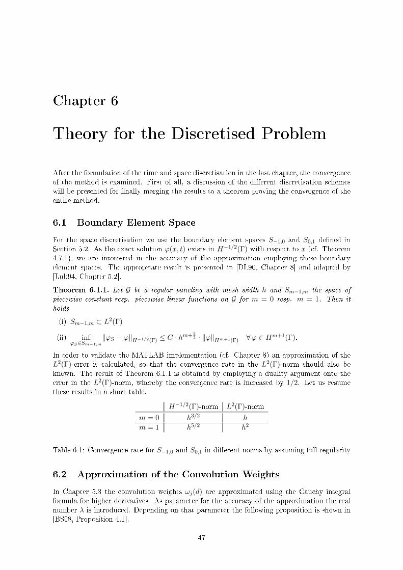
Chapter 6
Theory for the Discretised Problem
After the formulation of the time and space discretisation in the last chapter, the convergenceof the method is examined. First of all, a discussion of the dierent discretisation schemeswill be presented for nally merging the results to a theorem proving the convergence of theentire method.
6.1 Boundary Element Space
For the space discretisation we use the boundary element spaces S−1,0 and S0,1 dened inSection 5.2. As the exact solution ϕ(x, t) exists in H−1/2(Γ) with respect to x (cf. Theorem4.7.1), we are interested in the accuracy of the approximation employing these boundaryelement spaces. The appropriate result is presented in [DL90, Chapter 8] and adapted by[Lub94, Chapter 5.2].
Theorem 6.1.1. Let G be a regular paneling with mesh width h and Sm−1,m the space of
piecewise constant resp. piecewise linear functions on G for m = 0 resp. m = 1. Then it
holds
(i) Sm−1,m ⊂ L2(Γ)
(ii) infϕS∈Sm−1,m
‖ϕS − ϕ‖H−1/2(Γ) ≤ C · hm+ 3
2 · ‖ϕ‖Hm+1(Γ) ∀ϕ ∈ Hm+1(Γ).
In order to validate the MATLAB implementation (cf. Chapter 8) an approximation of theL2(Γ)-error is calculated, so that the convergence rate in the L2(Γ)-norm should also beknown. The result of Theorem 6.1.1 is obtained by employing a duality argument onto theerror in the L2(Γ)-norm, whereby the convergence rate is increased by 1/2. Let us resumethese results in a short table.
H−1/2(Γ)-norm L2(Γ)-norm
m = 0 h3/2 h
m = 1 h5/2 h2
Table 6.1: Convergence rate for S−1,0 and S0,1 in dierent norms by assuming full regularity
6.2 Approximation of the Convolution Weights
In Chapter 5.3 the convolution weights ωj(d) are approximated using the Cauchy integralformula for higher derivatives. As parameter for the accuracy of the approximation the realnumber λ is introduced. Depending on that parameter the following proposition is shown in[BS08, Proposition 4.1].
47
48 CHAPTER 6. THEORY FOR THE DISCRETISED PROBLEM
Proposition 6.2.1. Let N ∈ N, d > 0, ∆t = TN and λ < e−∆t be given. There exists a
constant C > 0 independent of the parameters, such that∣∣∣∣∣ω∆tj (d)− λ−j
N + 1
N∑l=0
Gκl(d)ζ−ljN+1
∣∣∣∣∣ ≤ Ce2T λN+1
d, for j = −N,−N + 1, . . . , N. (6.1)
The proof is based on the theory of discrete Fourier transform, mainly on the 'aliasing formula'[BS08, Theorem A.1], which gives a connection between the exact and the discrete Fouriercoecient.
6.3 Convergence of the Method
First of all, we consider the semi-discrete problem formulated in (5.4) using the BDF2 scheme.In [Lub94, Chapter 3] the author develops error estimates for the convolution quadratureapplied to convolutions of the form k(∂t)g. Starting with pointwise error bounds, using justthe properties of the linear multistep method and the bound (4.63) for the Laplace transformk, the theory leads to l2-error bounds. In [Lub94, Chapter 4] the theory is applied to thewave equation using the appropriate bound for V−1(s). [Lub94, Theorem 5.1] gives us theresult for an A-stable linear multistep method of order 2, that fulls furthermore an additionalcondition ([Lub94, Equation (3.11)]). As BDF2 has all these properties (cf. Section 3.7), wecan state the above cited theorem in the case using BDF2.
Theorem 6.3.1. Let the BDF2 method be employed for the time discretization. Consider
the problem on [0, T ] with equidistant discrete times n∆t where ∆t = TN for N ∈ N. For
g ∈ H50 (0, T ;H1/2(Γ)) the solution of the semi-discrete problem (5.4) denoted by ϕ∆t
n satises(∆t
N∑n=0
∥∥ϕ∆tn (·)− ϕ(·, n∆t)
∥∥2
H−1/2(Γ)
)≤ C∆t0 ·∆t2 · ‖g‖H5
0 (0,T ;H1/2(Γ)) (6.2)
uniformly for 0 < ∆t ≤ ∆t0 and a constant C∆t0 independent of ∆t and g.
As next step, in [Lub94, Chapter 5.2] the error caused by the discretisation in space by theGalerkin method is analysed. The result is a stability assertion and an error bound basedTheorem 6.1.1. The nal step in [Lub94] is merging the results, to get the convergence rate ofthe fully discretised problem (5.31). This is stated in [Lub94, Theorem 5.4] and is formulatedin [HKS09, Theorem 4.2] especially for the case of BDF2.
Theorem 6.3.2. For smooth compatible data g, i.e. g ∈ H50 (0, T ;H1/2(Γ)), the fully discrete
method dened by (5.31), i.e. Galerkin discretisation in space and operational convolution
quadrature in time, is unconditionally stable and provides a unique solution ϕ∆t,hn ∈ Sm−1,m
for m ∈ 0, 1 and 0 ≤ n ≤ N , which satises the error estimate∥∥∥ϕ(·, tn)− ϕ∆t,hn (·)
∥∥∥H−1/2(Γ)
≤ Cg(∆t2 + hm+ 32 ). (6.3)
In [HKS09] the authors continue to extend the convergence theory for perturbations in spacediscretization due to the approximation of the convolution weights and panel clustering. Theidea is to replace the weights for certain parameters d by zero. The condition for that is∣∣ω∆t
n (d)∣∣ ≤ ε
4πd, (6.4)
with ε > 0 the cuto parameter. The convergence theory is developed in [HKS09, Chapter4.2] and is once more achieved by examining the issue in the Laplace transformed case. The
6.3. CONVERGENCE OF THE METHOD 49
nal result (cf. [HKS09, Corollary 4.8]) is to choose ε ∼ h7m/2+25/4 to retain the originalconvergence rate.
The approximation of ω∆tn , developed in Section 5.3 and analysed in Section 6.2, is presented
in [BS08]. There the convergence theory is based on the result provided by 6.3.2, but witha slightly modied proof, and the error estimate given by Proposition 6.2.1. The accuracyparameter is λ instead of ε. Putting all these results together allows to proof the main result[BS08, Theorem 5.1].
Theorem 6.3.3. Let the exact solution ϕ(·, t) be in Hm+1(Γ) for any t ∈ [0, T ], the data
g ∈ H50 (0, T ;H1/2(Γ)) and the boundary element space S = Sm−1,m for m ∈ 0, 1. For a
given σ > 0 and for λ < 1 such that λN+1 ≤ Cσe−(2+σ)T (1− e−σ∆t)h∆t2, the solution ϕ∆t,h
n
for the problem (5.54) exists and satises the error estimate∥∥∥ϕ∆t,hn − ϕ(·, tn)
∥∥∥H−1/2(Γ)
≤ Cg(tn)(λN+1e2Th−1∆t−5 + ∆t2 + hm+3/2), (6.5)
where Cσ depends on σ and Cg depends on σ and the right-hand side g.
To resume this result in a short, recipe-style way, we state
Corollary 6.3.4. Assume the same conditions of the last theorem and let
hm+3/2 . ∆t2, λN+1 ∼ h7m/2+25/4, (6.6)
then the optimal rate of convergence is achieved,∥∥∥ϕ∆t,hn − ϕ(·, tn)
∥∥∥H−1/2(Γ)
≤ C∆t2, (6.7)
with C depending on g.

50 CHAPTER 6. THEORY FOR THE DISCRETISED PROBLEM
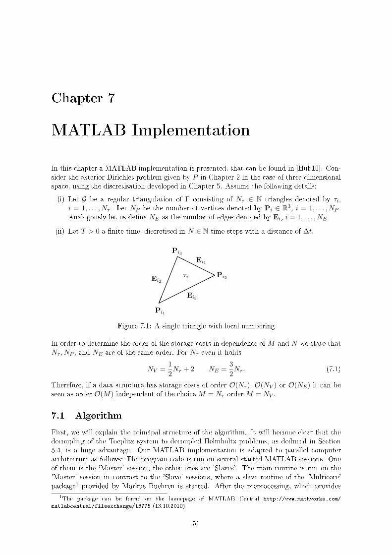
Chapter 7
MATLAB Implementation
In this chapter a MATLAB implementation is presented, that can be found in [Hub10]. Con-sider the exterior Dirichlet problem given by P in Chapter 2 in the case of three dimensionalspace, using the discretisation developed in Chapter 5. Assume the following details:
(i) Let G be a regular triangulation of Γ consisting of Nτ ∈ N triangles denoted by τi,i = 1, . . . , Nτ . Let NP be the number of vertices denoted by Pi ∈ R3, i = 1, . . . , NP .Analogously let us dene NE as the number of edges denoted by Ei, i = 1, . . . , NE .
(ii) Let T > 0 a nite time, discretised in N ∈ N time steps with a distance of ∆t.
HH
HHH
H
Pi1
Pi2
Pi3
Ei1
Ei2
Ei3
τi
Figure 7.1: A single triangle with local numbering
In order to determine the order of the storage costs in dependence of M and N we state thatNτ , NP , and NE are of the same order. For Nτ even it holds
NV =1
2Nτ + 2 NE =
3
2Nτ . (7.1)
Therefore, if a data structure has storage costs of order O(Nτ ), O(NV ) or O(NE) it can beseen as order O(M) independent of the choice M = Nτ order M = NV .
7.1 Algorithm
First, we will explain the principal structure of the algorithm. It will become clear that thedecoupling of the Toeplitz system to decoupled Helmholtz problems, as deduced in Section5.4, is a huge advantage. Our MATLAB implementation is adapted to parallel computerarchitecture as follows: The program code is run on several started MATLAB sessions. Oneof them is the 'Master' session, the other ones are 'Slaves'. The main routine is run on the'Master' session in contrast to the 'Slave' sessions, where a slave routine of the 'Multicore'package1 provided by Markus Buehren is started. After the preprocessing, which provides
1The package can be found on the homepage of MATLAB Central http://www.mathworks.com/
matlabcentral/fileexchange/13775 (13.10.2010)
51
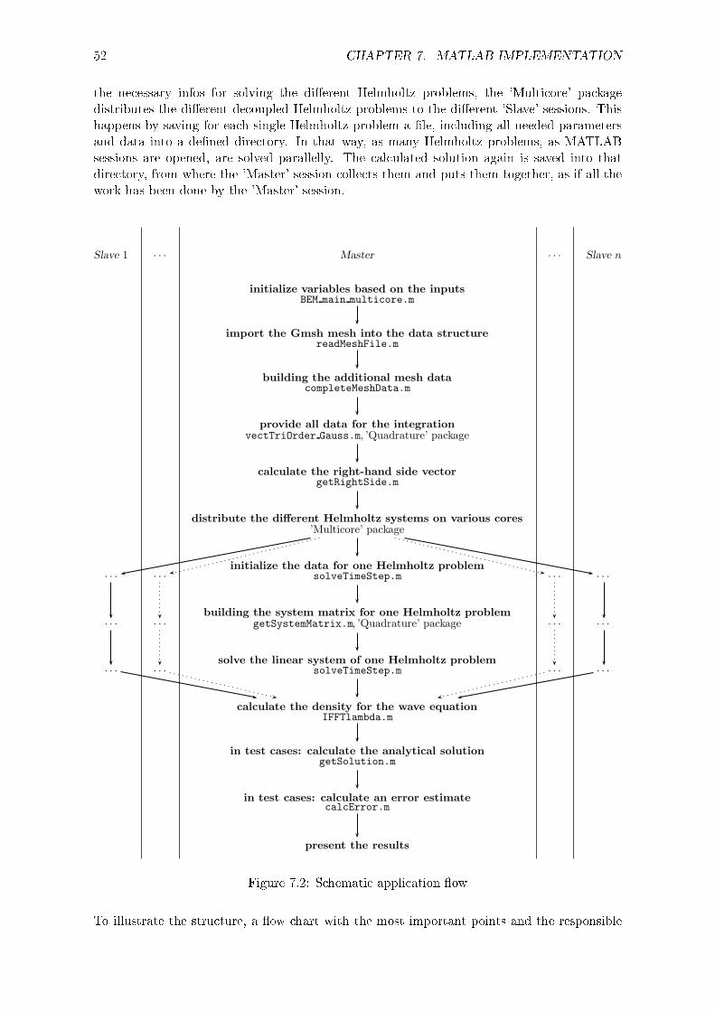
52 CHAPTER 7. MATLAB IMPLEMENTATION
the necessary infos for solving the dierent Helmholtz problems, the 'Multicore' packagedistributes the dierent decoupled Helmholtz problems to the dierent 'Slave' sessions. Thishappens by saving for each single Helmholtz problem a le, including all needed parametersand data into a dened directory. In that way, as many Helmholtz problems, as MATLABsessions are opened, are solved parallelly. The calculated solution again is saved into thatdirectory, from where the 'Master' session collects them and puts them together, as if all thework has been done by the 'Master' session.
Slave 1 · · · Master · · · Slave n
initialize variables based on the inputsBEM main multicore.m
import the Gmsh mesh into the data structurereadMeshFile.m
building the additional mesh datacompleteMeshData.m
provide all data for the integrationvectTriOrder Gauss.m, ’Quadrature’ package
calculate the right-hand side vectorgetRightSide.m
distribute the different Helmholtz systems on various cores’Multicore’ package
· · · · · ·
initialize the data for one Helmholtz problemsolveTimeStep.m · · · · · ·
· · · · · ·
building the system matrix for one Helmholtz problemgetSystemMatrix.m, ’Quadrature’ package · · · · · ·
· · · · · ·
solve the linear system of one Helmholtz problemsolveTimeStep.m · · · · · ·
calculate the density for the wave equationIFFTlambda.m
in test cases: calculate the analytical solutiongetSolution.m
in test cases: calculate an error estimatecalcError.m
present the results
Figure 7.2: Schematic application ow
To illustrate the structure, a ow chart with the most important points and the responsible
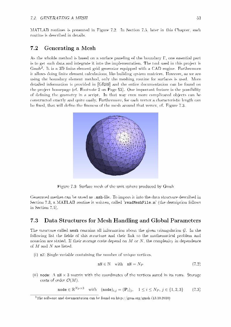
7.2. GENERATING A MESH 53
MATLAB routines is presented in Figure 7.2. In Section 7.5, later in this Chapter, eachroutine is described in details.
7.2 Generating a Mesh
As the wholde method is based on a surface paneling of the boundary Γ, one essential partis to get such data and integrate it into the implementation. The tool used in this project isGmsh2. It is a 3D nite element grid generator equipped with a CAD engine. Furthermoreit allows doing nite element calculations, like building system matrices. However, as we areusing the boundary element method, only the meshing routine for surfaces is used. Moredetailed information is provided in [GR09] and the entire documentation can be found onthe project homepage (cf. Footnote 2 on Page 53). One important feature is the possibilityof dening the geometry in a script. In that way even more complicated objects can beconstructed exactly and quite easily. Furthermore, for each vertex a characteristic length canbe xed, that will dene the neness of the mesh around that vertex, cf. Figure 7.3.
Figure 7.3: Surface mesh of the unit sphere produced by Gmsh
Generated meshes can be saved as .msh-le. To import it into the data structure described inSection 7.3, a MATLAB routine is written, called 'readMeshFile.m' (the description followsin Section 7.5).
7.3 Data Structures for Mesh Handling and Global Parameters
The structure called mesh contains all information about the given triangulation G. In thefollowing list the elds of this structure and their link to the mathematical problem andnotation are stated. If their storage costs depend on M or N , the complexity in dependenceof M and N are listed.
(i) nN: Single variable containing the number of unique vertices.
nN ∈ N with nN = NP (7.2)
(ii) node: A nN × 3 matrix with the coordinates of the vertices saved in its rows. Storagecosts of order O(M).
node ∈ RNP×3 with (node)i,j = (Pi)j , 1 ≤ i ≤ NP , j ∈ 1, 2, 3 (7.3)
2The software and documentation can be found on http://geuz.org/gmsh (13.10.2010)
54 CHAPTER 7. MATLAB IMPLEMENTATION
(iii) nT: Single variable containing the number of unique triangles.
nT ∈ N with nT = Nτ (7.4)
(iv) triangle: A nT× 3 matrix with indices of the vertices saved in its rows. Storage costsof order O(M).
triangle ∈ NNτ×3 with (7.5)
τi = conv
P(triangle)i,1 ,P(triangle)i,2 ,P(triangle)i,3
(7.6)
(v) nE: Single variable containing the number of unique edges.
nE ∈ N with nE = NE (7.7)
(vi) edgeind: A nE× 2 matrix with indices of the starting and end vertex of a unique edge.Storage costs of order O(M).
edgeind ∈ NNE×2 (7.8)
For a i ∈ 1, . . . , NE, assume that Ei is the j-th edge of a triangle τk, 1 ≤ j ≤ 3,1 ≤ k ≤ Nτ . Then it holds
j = 1 : (edgeind)i,l | l = 1, 2 = (triangle)k,2, (triangle)k,3 (7.9)
j = 2 : (edgeind)i,l | l = 1, 2 = (triangle)k,3, (triangle)k,1 (7.10)
j = 3 : (edgeind)i,l | l = 1, 2 = (triangle)k,1, (triangle)k,2 (7.11)
Furthermore
(edgeind)i,1 < (edgeind)i,2 ∀ i ∈ 1, . . . , NE (7.12)
(vii) edge: A nE× 3 matrix with coordinates of the edges saved in its rows. Storage costs oforder O(M).
edge ∈ RNE×3 (7.13)
Assume that edge Ei consists of vertices Pj and Pk with 1 ≤ j < k ≤ NP and i ∈1, . . . , NE. Then
(edge)i,l = (Pk)l − (Pj)l, 1 ≤ l ≤ 3 (7.14)
(viii) triangletoedge: A nT × 3 matrix with indices of the edges of a triangle. The sign ofthe entry shows the orientation of the edge. Storage costs of order O(M).
triangletoedge ∈ ZNτ×3 (7.15)
For 1 ≤ i ≤ Nτ and 1 ≤ j ≤ 3 let x = (triangletoedge)i,j be an entry. Then it holds
j = 1 : (edge)|x|,∗ =
(
(triangle)i,2 (triangle)i,3
)x > 0(
(triangle)i,3 (triangle)i,2
)x < 0
(7.16)
j = 2, 3 analogously to the cases in (7.10) and (7.11) (7.17)
7.3. DATA STRUCTURES FOR MESH HANDLING AND GLOBAL PARAMETERS 55
(ix) area: A nT array with the area of the triangles saved in it. Storage costs of order O(M).
area ∈ RNτ with (area)i = |τi|, ∀ i ∈ 1, . . . , Nτ (7.18)
Assume A,B ∈ R3 are two dierent edges of the triangle τ , available in edge. Then thearea is calculated by
|τ | = 1
2‖A×B‖, (7.19)
where ‖·‖ is the Euclidean norm and × the cross product in R3.
(x) edgelength: A nE array with Euclidean length of the edges saved in it. Storage costsof order O(M).
edgelength ∈ RNE with (edgelength)i = ‖Ei‖ ∀ i ∈ 1, . . . , NE (7.20)
(xi) diameter: A nT array with the diameter of the triangles saved in it. Storage costs oforder O(M).
diameter ∈ RNτ with (diameter)i = maxx,y∈τi
‖x− y‖ ∀ i ∈ 1, . . . , Nτ (7.21)
In the case of at triangles with straight edges, the diameter is equal to the largestdistance between two vertices of the triangle. Let 1 ≤ j1 < j2 < j3 ≤ NE be the indicesof the edges of a triangle τi, i ∈ 1, . . . , Nτ. Then
(diameter)i = max‖Ej1‖, ‖Ej2‖, ‖Ej3‖ (7.22)
(xii) hmin, hmax: Single variables containing the minimal resp. maximal diameter of thetriangulation G. Using the considerations made for diameter it holds
hmin, hmax ∈ R with hmin = min1≤i≤NE
‖Ei‖ resp. hmax = max1≤i≤NE
‖Ei‖ (7.23)
(xiii) enumeration: A nT× nT sparse matrix encoding the relation of two triangles as a ag.Storage costs of order O(M2).Furthermore enumeration is symmetric and it holds
enumeration ∈ NNτ×Nτ with 1 ≤ i, j ≤ Nτ (7.24)
(enumeration)i,j = (enumeration)j,i =
0 the distance between τi and τj is positive
1 τi and τj have a common vertex
2 τi and τj have a common edge
3 τi and τj are identical
(7.25)
(xiv) index: A nT× nT sparse matrix saving the local number of a common object. Storagecosts of order O(M2).
index ∈ NNτ×Nτ with 1 ≤ i, j ≤ Nτ (7.26)
(index)i,j =
0 (enumeration)i,j = 0
k ∈ 1, 2, 3 (enumeration)i,j = 1 and k is the local number
of the common vertex w.r.t. τi
k ∈ 1, 2, 3 (enumeration)i,j = 2 and k is the local number
of the common edge w.r.t. τi
0 (enumeration)i,j = 3
(7.27)
This matrix is not symmetric, however the positioning of non-zero entries is symmetric.
56 CHAPTER 7. MATLAB IMPLEMENTATION
(xv) distnode: A nN × nN matrix with the distance between the nodes saved in it. Storagecosts of order O(M2).
distnode ∈ RNP×NP with (distnode)i,j = ‖Pi −Pj‖ ∀ i, j ∈ 1, . . . , NP (7.28)
(xvi) distance: A nT × nT matrix with an estimate of the distance between two trianglessaved in it. Storage costs of order O(M2).
distance ∈ RNτ×Nτ with (distance)i,j = maxx∈τi,y∈τj
‖x− y‖, ∀ i, j ∈ 1, . . . , Nτ
(7.29)
As the right-hand side in (7.29) is relatively time consuming in the computation, weemploy an upper bound instead.
(distance)i,j = maxA is vertex of τiB is vertex of τj
‖A−B‖ ∀ i, j ∈ 1, . . . , Nτ (7.30)
(xvii) edgetotriangle: A nE × 2 matrix with the indices of its adjacent triangles stored inits rows. Storage costs of order O(M).
edgetotriangle ∈ NNE×2 (7.31)
Assume, that Ei is a joint edge of two triangles τj , τk, for i ∈ 1, . . . , NE, j, k ∈1, . . . , Nτ and j 6= k, then
(edgetotriangle)i,1, (edgetotriangle)i,2 = j, k (7.32)
(xviii) midpoint: A nT × 3 matrix with the coordinates of the midpoint of every trianglesaved in its rows. Storage costs of order O(M).
midpoint ∈ RNτ×3 (7.33)
Assume, that A,B,C ∈ R3 are the vertices of a triangle τi, i ∈ 1, . . . , Nτ. Hence
(midpoint)i,l =1
3(Al + Bl + Cl) ∀ l ∈ 1, 2, 3 (7.34)
−→ Overall the structure mesh uses storage of the order O(M2).
The parameters of the discretisation, which are independent of the mesh geometry, are savedin a structure called param. This structure contains
(i) T: A single variable that represents the nal time.
T ∈ R with T = T (7.35)
(ii) N, N1: Two single variables saving the number of time steps.
N, N1 ∈ N with N = N, N1 = N + 1 (7.36)
(iii) dt: A single variable that represents the length of a time step.
dt ∈ R with dt = ∆t (7.37)
7.3. DATA STRUCTURES FOR MESH HANDLING AND GLOBAL PARAMETERS 57
(iv) filename: A string containing the name of the mesh le generated by Gmsh.
(v) order: A ag saving the boundary element space.
order ∈ N with order =
0 approximation using piecewise constant elements
1 approximation using piecewise linear elements
(7.38)
(vi) dof: A single variable representing the number of degree of freedom with respect to thespace discretisation.
dof ∈ N with dof =
Nτ approximation using piecewise constant elements
NP approximation using piecewise linear elements
(7.39)
(vii) zeta: A single complex variable used for computing the wavenumbers.
zeta ∈ C with zeta = ζN+1 = e−2πiN+1 (7.40)
(viii) lambda: A single variable representing a parameter for approximating the convolutionweights used in Section 5.3
lambda ∈ (0, 1) with lambda = λ (7.41)
(ix) kappal: A N1 array consisting of all wave numbers for the decoupled systems. Storagecosts of order O(N).
kappal ∈ CN+1 with (kappal)l+1 = iγ(λζ lN+1)
∆t, l ∈ 0, . . . , N (7.42)
with γ the quotient of the generating polynomials of BDF2.
(x) testCase: A single ag for the choice of implemented test cases, which determine theright-hand side function g.
testCase ∈ N with (7.43)
testCase =
0 test case with e(x) = Y 00 (x) (cf. Section 8.1)
1 test case with e(x) = Y 11 (x) (cf. Section 8.1)
2 simple version of a plane wave (cf. Section 8.5)
3 extended version of a plane wave (cf. Section 8.5)
4 spherical wave (cf. Section 8.5)
(7.44)
(xi) intlogh: A single ag for the choice of the number of Gauss points for the numericalquadrature.
intlogh ∈ true, false with intlogh =
true using the rules of Section 7.4
false use the same number of Gausspoints for all combinations
(7.45)
−→ Overall the structure param uses storage of the order O(N).
Both described structures are declared as global variables. Therefore they will not be part ofany input or output of the routines described in Section 7.5.
58 CHAPTER 7. MATLAB IMPLEMENTATION
7.4 Numerical Integration
The numerical integration for calculating the system matrices and the right-hand side vectorfor the decoupled systems (5.56) is based on the integration routines developed in [SS04,Chapter 5]. The fundamental solution of the Helmholtz equation is an example of the classof kernel functions, for which these routines are developed [SS04, Example 5.1.17].
As the entry of a system matrix, according to (5.55), can be written as
(Al)k,m =
∫Γ
∫ΓGκl(‖x− y‖)bm(y)bk(x)dΓydΓx =
∑τ∈G
∑t∈G
∫τ
∫t. . . dΓydΓx, (7.46)
where 0 ≤ l ≤ N and 1 ≤ k,m ≤M , the methods have to be developed just for the integrationover a pair of triangles τ × t for τ, t ∈ G. As
Gκl(x,y) =eiκl‖x−y‖
4π‖x− y‖, (7.47)
is singular if τ ∩ t 6= ∅ or nearly singular for a small distance between τ and t, specialroutines have to be developed to calculate the matrix entries eciently and exactly enough.As mentioned above, this is done in [SS04]. Here only the most important points are recalled:
(i) Using the transformations χτ resp. χt, the integration over a pair of triangles τ × t ispulled back to the reference element τ × τ , where the quadrature routine is developed .
(ii) Relative coordinates z = x − y are introduced to x the singularity ‖x− y‖ at theorigin. Then an ε neighbourhood is cut out and a 'good', in the sense of appropriateto the properties of the integral kernel, decomposition of the integration domain ischosen. After changing the integration order, the integration domain is transferredto the four dimensional simplex. Finally the integration domain is transformed on[0, 1]4. Furthermore it is shown, that in each former singular case, the integrand can beanalytically extended onto a complex neighbourhood of [0, 1]4.
(iii) The resulting regularizing coordinate transforms require only some mild assumptions onthe parametrization of the two triangles.
The assumptions mentioned in Point (iii) are the following.
Assumption 7.4.1. Let be τ, t ∈ G and χτ resp. χt their parametrizations. It holds:
(i) In the case of identical panels: χτ = χt.
(ii) In the case of a common edge: χτ (s, 0) = χt(s, 0) for all s ∈ [0, 1].
(iii) In the case of a common vertex: χτ (0, 0) = χt(0, 0).
To assert that the triangles are arranged in exactly that manner is one of the most importantand most sensitive parts of the implementation.
Furthermore, let us dene the integrand in local coordinates
kloc(x, y) = bm(y)bm(x)k(χτ (x), χt(y))gτ (x)gt(y), (7.48)
where gτ resp. gt denotes the Gramian Determinant of χτ resp. χt.
gτ (x) =√
det(Dχτ (x))T (Dχτ (x)). (7.49)
7.4. NUMERICAL INTEGRATION 59
Under these assumptions we have the following regularizing transforms:
• Identical Panels:
Iτ×t =
∫(0,1)4
ξ3η21η2
klocξ
11− η1 + η1η2
1− η1η2η31− η1
+ kloc
ξ
1− η1η2η3
1− η1
11− η1 + η1η2
+kloc
ξ
1η1(1− η2 + η2η3)
1− η1η2
η1(1− η2)
+ kloc
ξ
1− η1η2
η1(1− η2)1
η1(1− η2η2η3
+ kloc
ξ
1− η1η2η3
η1(1− η2η3)1
η1(1− η2)
+ kloc
ξ
1η1(1− η2)1− η1η2η3
η1(1− η2η3
dη1dη2dη3dξ
(7.50)
• Common Edge:
Iτ×t =
∫(0,1)4
ξ3η21kloc
ξ
ξη1η3
ξ(1− η1η2)ξη1(1− η2)
+ ξ3η21η2
kloc
ξξη1
ξ(1− η1η2η3)ξη1η2(1− η3)
+ kloc
ξ(1− η1η2)ξη1(1− η2)
ξξη1η2η3
+ kloc
ξ(1− η1η2η3)ξη1η2(1− η3)
ξξη1
+ kloc
ξ(1− η1η2η3)ξη1(1− η2η3)
ξξη1η2
dη1dη2dη3dξ
(7.51)
• Common Vertex or Positive Distance:
Iτ×t =
∫(0,1)4
ξ3η2kloc(ξ, ξη1, ξη2, ξη2η3) + kloc(ξη2, ξη2η3, ξ, ξη1)dη1dη2dη3dξ. (7.52)
As we now have an analytic integrand f : [0, 1]4 → C, we can employ a tensorised Gaussquadrature on it. That means, that the exact integral
I(f) :=
∫(0,1)4
f(x)dx, (7.53)
is approximated by a quadrature of the form
Qn(f) =
n1∑i=1
n2∑j=1
n3∑k=1
n4∑l=1
ωi,n1ωj,n2ωk,n3ωl,n4f(ξi,n1 , ξj,n2 , ξk,n3 , ξl,n4), (7.54)
with n = (n1, n2, n3, n4)T ∈ N4. Furthermore ωi,n resp. ξi,n for n ∈ N and 1 ≤ i ≤ n are theweights resp. nodes for the Gauss quadrature of order n on [0, 1]. They can be calculated oncefor dierent n to a high precision and can be saved in a le, for using it in each quadrature.
In [SS04, Chapter 5] the analysis of the quadrature error and the question, how n has to bechosen that the quadrature error does not spoil the convergence rate of a Galerkin boundaryelement method is developed. The practical results are presented in [SS04, Chapter 5.3.4]. Inthe case of the Helmholtz problem, where the single layer potential denes a boundary integraloperator from H−1/2(Γ) to H1/2(Γ) and induces an integral equation of negative order, weget the following result.
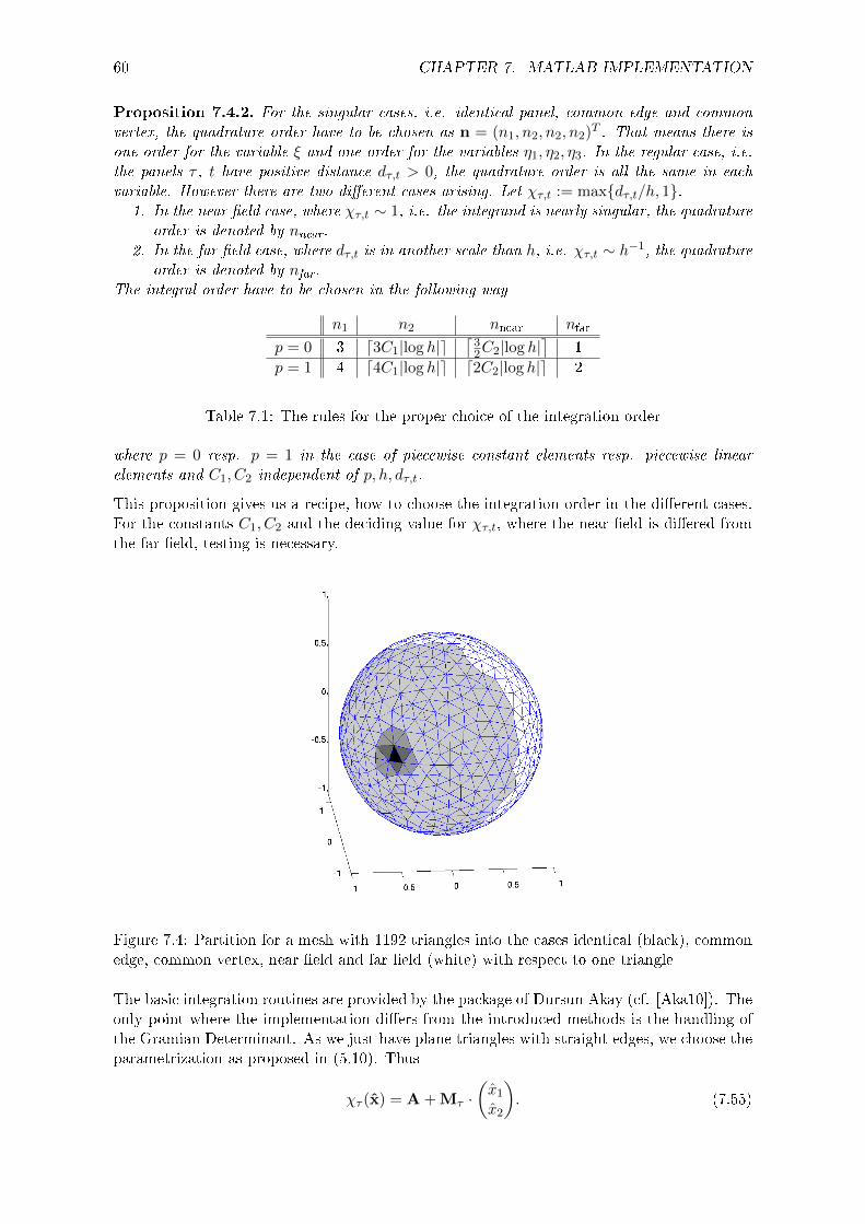
60 CHAPTER 7. MATLAB IMPLEMENTATION
Proposition 7.4.2. For the singular cases, i.e. identical panel, common edge and common
vertex, the quadrature order have to be chosen as n = (n1, n2, n2, n2)T . That means there is
one order for the variable ξ and one order for the variables η1, η2, η3. In the regular case, i.e.
the panels τ , t have positive distance dτ,t > 0, the quadrature order is all the same in each
variable. However there are two dierent cases arising. Let χτ,t := maxdτ,t/h, 1.1. In the near eld case, where χτ,t ∼ 1, i.e. the integrand is nearly singular, the quadrature
order is denoted by nnear.2. In the far eld case, where dτ,t is in another scale than h, i.e. χτ,t ∼ h−1, the quadrature
order is denoted by nfar.The integral order have to be chosen in the following way
n1 n2 nnear nfar
p = 0 3 d3C1|log h|e⌈
32C2|log h|
⌉1
p = 1 4 d4C1|log h|e d2C2|log h|e 2
Table 7.1: The rules for the proper choice of the integration order
where p = 0 resp. p = 1 in the case of piecewise constant elements resp. piecewise linear
elements and C1, C2 independent of p, h, dτ,t.
This proposition gives us a recipe, how to choose the integration order in the dierent cases.For the constants C1, C2 and the deciding value for χτ,t, where the near eld is diered fromthe far eld, testing is necessary.
Figure 7.4: Partition for a mesh with 1192 triangles into the cases identical (black), commonedge, common vertex, near eld and far eld (white) with respect to one triangle
The basic integration routines are provided by the package of Dursun Akay (cf. [Aka10]). Theonly point where the implementation diers from the introduced methods is the handling ofthe Gramian Determinant. As we just have plane triangles with straight edges, we choose theparametrization as proposed in (5.10). Thus
χτ (x) = A + Mτ ·(x1
x2
). (7.55)
7.5. ROUTINES 61
Therefore, it holds Dχτ (x) = Mτ , that is independent of x. Hence gτ (x) is a constant.More precisely, the columns of Mτ contain the coordinates of two dierent edge-vectors ofthe triangle τ . Let us denote them as E and F. Therefore we have
g2τ = det
(− E −− F −
)·
| |E F| |
= det
(‖E‖2 〈E,F〉〈F,E〉 ‖F‖2
)(7.56)
= ‖E‖2‖F‖2 − 〈E,F〉2, (7.57)
where 〈·, ·〉 is the Euclidean scalar product in R3 and ‖·‖ the Euclidean norm. Using Lagrange'sidentity leads to
g2τ = ‖E‖2‖F‖2 − 〈E,F〉2 = 〈E× F,E× F〉 = ‖E× F‖2 (7.58)
= 4|τ |2, (7.59)
where × is the outer product on R3 and |τ | the measure of τ . Thus, instead of calculating gτ ,one can determine the area of τ and use the representation
gτ = 2|τ |. (7.60)
7.5 Routines
The program ow of the implementation is presented in Section 7.1. In this section the singleroutines are documented. Instead of giving a detailed description of the implementation, themain principles used for coding are presented at the beginning. Apart from these principlesthe implementation is straight forward and further details can be found in the commentedcode. Technical diculties arise especially in the handling of the mesh information. However,that issue is presented in details in the Section 7.5.1.
Everywhere in the discretisation, nite sums or equations appear which have to be satisedfor various nite parameters. The for-loops are a straight forward way to implement suchsums. However MATLAB oers a powerful way to speed up the program by avoiding theseloops. This concept is called vectorization. The MATLAB documentation gives a few simpleillustrating examples for that concept. The fundamental idea is to transform a non-recursiveloop into a vector operation. The entries of the vector represent the dierent steps of theloop. The gain of speed is in many cases striking. Furthermore, various MATLAB routinesare already programmed in a vectorized way, e.g. the fast Fourier transform fft, that canapply the transform on dierent vectors simultaneously.Strongly linked to the vectorization is the concept of linear indexing. As each m× n matrixA can be identied by a vector with m ·n entries, vectorization also can be applied to matrixoperations. In MATLAB linear indexing is done in the following way
A =
a11 · · · a1n...
...am1 · · · amn
, (7.61)
is identied with the vector(a11 · · · am1 a12 · · · am2 · · · a1n · · · amn
). (7.62)
Hence the entry in the matrix at the index (i, j) is identied with entry in the vector withindex i+ (j − 1) ·m. Therefore the same concepts as for vectors can be applied to matrices.The implementation makes use of these concepts as often as possible. As mentioned, theimpact on the performance is substantial. However, the readability of the code suers fromthat, as it is not clear at rst glance, which values are assigned to which variable.
62 CHAPTER 7. MATLAB IMPLEMENTATION
7.5.1 Arranging the Pairs of Triangles
In the preprocessing phase of the algorithm, i.e. before the dierent Helmholtz problems aredistributed to dierent processors, the set of triangles for the integration is prepared. Asstated in Assumption 7.4.1, the parametrizations of the triangles play an important role, asthe regularizing transformations depend on the geometry and the explicit parametrizations.Hence for an integration
∫τ
∫t . . . for τ, t ∈ G, where τ ∩ t 6= ∅, the local numbering of the
vertices of the triangles τ and t has to be arranged properly in order to fulll Assumption 7.4.1.Due to the fact that for each Helmholtz problem the same integration domains τ × t arise,and to be able to eect the integration in a vectorized way, all possible triangle combinationsare prepared in advance.
Using the fact that all system matrices dened by (5.55) are symmetric but non-hermitian, dueto the symmetry of the integration kernels respectively the imaginary entries on the diagonal,only pairs of triangles of the form τi × τj with 1 ≤ i ≤ j ≤ Nτ have to be considered. Thatdoes not reduce the computational complexity order, but halves the time for the computationand the memory requirement. The symmetry is taken into account by assigning the calculatedintegrals to the system matrices Al, i.e. the values are assigned to (Al)k,m as well as (Al)m,k.
The result of this preparation are two L × 3 matrices triangle1 and triangle2, saved in
the structure quadrature, where L = N2τ+Nτ
2 . In the l-th row of these two matrices thelocal numbering of the vertices of the triangles τ, t ∈ G are saved, arranged in the way thatAssumption 7.4.1 is fullled. This arrangement is once more done in vectorized form in thele vectTriOrder_Gauss.m. The structure quadrature has therefore storage costs of orderO(M2).
7.5.2 Calculating the System Matrices
The fundamental part of the algorithm is to calculate the entries of the system matrices Al.They are given by (5.55) as
(Al)k,m =
∫Γ
∫ΓGκl(‖x− y‖)bm(y)bk(x)dΓydΓx, (7.63)
for 0 ≤ l ≤ N and 1 ≤ k,m ≤ M . Let us look at the calculation of these entries for thedierent approximation spaces dened in Section 5.2.
(i) Recall that in the case of piecewise constant functions the basis functions bm are thecharacteristic functions for the triangles τm. Therefore, the integral over Γ× Γ reducesto
(Al)k,m =
∫τk
∫τm
Gκl(‖x− y‖)dΓydΓx, (7.64)
i.e., an integral over a pair of triangles. That leads to the algorithm
for 1 ≤ k,m ≤M (Al)k,m =
∫τk
∫τmGκl(‖x− y‖)dΓydΓx
end
To avoid the double for-loop, the quadrature package is built to handle the calculationof several entries at once by using the built-in vectorization.
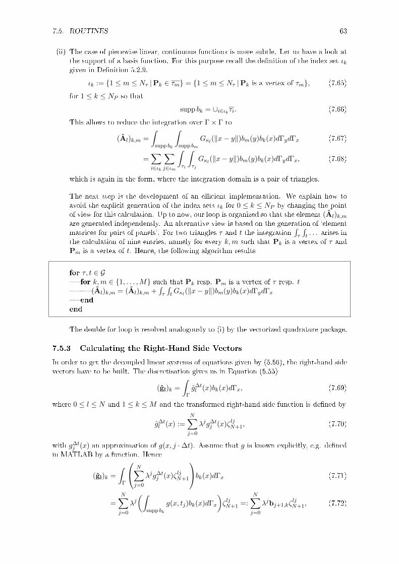
7.5. ROUTINES 63
(ii) The case of piecewise linear, continuous functions is more subtle. Let us have a look atthe support of a basis function. For this purpose recall the denition of the index set ιkgiven in Denition 5.2.9.
ιk := 1 ≤ m ≤ Nτ |Pk ∈ τm = 1 ≤ m ≤ Nτ |Pk is a vertex of τm, (7.65)
for 1 ≤ k ≤ NP so that
supp bk = ∪i∈ιkτi. (7.66)
This allows to reduce the integration over Γ× Γ to
(Al)k,m =
∫supp bk
∫supp bm
Gκl(‖x− y‖)bm(y)bk(x)dΓydΓx (7.67)
=∑i∈ιk
∑j∈ιm
∫τi
∫τj
Gκl(‖x− y‖)bm(y)bk(x)dΓydΓx, (7.68)
which is again in the form, where the integration domain is a pair of triangles.
The next step is the development of an ecient implementation. We explain how toavoid the explicit generation of the index sets ιk for 0 ≤ k ≤ NP by changing the pointof view for this calculation. Up to now, our loop is organized so that the element (Al)k,mare generated independently. An alternative view is based on the generation of 'elementmatrices for pairs of panels'. For two triangles τ and t the integration
∫τ
∫t . . . arises in
the calculation of nine entries, namely for every k,m such that Pk is a vertex of τ andPm is a vertex of t. Hence, the following algorithm results
for τ, t ∈ G for k,m ∈ 1, . . . ,M such that Pk resp. Pm is a vertex of τ resp. t (Al)k,m = (Al)k,m +
∫τ
∫tGκl(‖x− y‖)bm(y)bk(x)dΓydΓx
end
end
The double for-loop is resolved analogously to (i) by the vectorized quadrature package.
7.5.3 Calculating the Right-Hand Side Vectors
In order to get the decoupled linear systems of equations given by (5.56), the right-hand sidevectors have to be built. The discretisation gives us in Equation (5.55)
(gl)k =
∫Γg∆tl (x)bk(x)dΓx, (7.69)
where 0 ≤ l ≤ N and 1 ≤ k ≤M and the transformed right-hand side function is dened by
g∆tl (x) :=
N∑j=0
λjg∆tj (x)ζ ljN+1, (7.70)
with g∆tj (x) an approximation of g(x, j ·∆t). Assume that g is known explicitly, e.g. dened
in MATLAB by a function. Hence
(gl)k =
∫Γ
N∑j=0
λjg∆tj (x)ζ ljN+1
bk(x)dΓx (7.71)
=
N∑j=0
λj(∫
supp bk
g(x, tj)bk(x)dΓx
)ζ ljN+1 =:
N∑j=0
λjbj+1,kζljN+1, (7.72)
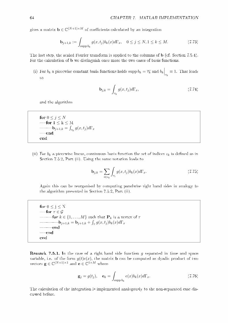
64 CHAPTER 7. MATLAB IMPLEMENTATION
gives a matrix b ∈ C(N+1)×M of coecients calculated by an integration
bj+1,k :=
∫supp bk
g(x, tj)bk(x)dΓx, 0 ≤ j ≤ N, 1 ≤ k ≤M. (7.73)
The last step, the scaled Fourier transform is applied to the columns of b (cf. Section 7.5.4).For the calculation of b we distinguish once more the two cases of basis functions.
(i) For bk a piecewise constant basis functions holds supp bk = τk and bk
∣∣∣τk≡ 1. That leads
to
bj,k =
∫τk
g(x, tj)dΓx, (7.74)
and the algorithm
for 0 ≤ j ≤ N for 1 ≤ k ≤ M bj+1,k =
∫τkg(x, tj)dΓx
end
end
(ii) For bk a piecewise linear, continuous basis function the set of indices ιk is dened as inSection 7.5.2, Part (ii). Using the same notation leads to
bj,k =∑i∈ιk
∫τi
g(x, tj)bk(x)dΓx. (7.75)
Again this can be reorganised by computing panelwise right-hand sides in analogy tothe algorithm presented in Section 7.5.2, Part (ii).
for 0 ≤ j ≤ N for τ ∈ G for k ∈ 1, . . . ,M such that Pk is a vertex of τ bj+1,k = bj+1,k +
∫τ g(x, tj)bk(x)dΓx
end
end
end
Remark 7.5.1. In the case of a right-hand side function g separated in time and spacevariable, i.e. of the form g(t)e(x), the matrix b can be computed as dyadic product of twovectors g ∈ C(N+1)×1 and e ∈ C1×M where
gj = g(tj), ek =
∫supp bk
e(x)bk(x)dΓx. (7.76)
The calculation of the integration is implemented analogously to the non-separated case dis-cussed before.
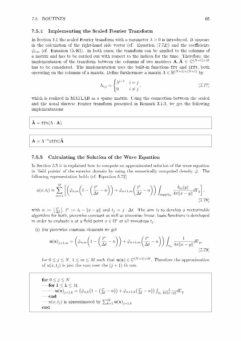
7.5. ROUTINES 65
7.5.4 Implementing the Scaled Fourier Transform
In Section 3.1 the scaled Fourier transform with a parameter λ > 0 is introduced. It appearsin the calculation of the right-hand side vector (cf. Equation (7.72)) and the coecientsϕl,m (cf. Equation (5.46)). In both cases, the transform can be applied to the columns ofa matrix and has to be carried out with respect to the indices for the time. Therefore, theimplementation of the transform between the columns of two matrices A, A ∈ C(N+1)×M
has to be considered. The implementation uses the built-in functions fft and ifft, bothoperating on the columns of a matrix. Dene furthermore a matrix Λ ∈ R(N+1)×(N+1) by
Λi,j =
λi−1 i = j
0 i 6= j, (7.77)
which is realized in MATLAB as a sparse matrix. Using the connection between the scaledand the usual discrete Fourier transform presented in Remark 3.1.3, we get the followingimplementations
A = fft(Λ ·A)
A = Λ−1ifft(A
7.5.5 Calculating the Solution of the Wave Equation
In Section 5.5 it is explained how to compute an approximated solution of the wave equationin 'eld points' of the exterior domain by using the numerically computed density ϕ. Thefollowing representation holds (cf. Equation 5.72)
u(x, tl) ≈M∑m=1
[(ϕn,m
(1−
(t∗
∆t− n
))+ ϕn+1,m
(t∗
∆t− n
))∫supp bm
bm(y)
4π‖x− y‖dΓy
],
(7.78)
with n :=⌊t∗
∆t
⌋, t∗ := tl − ‖x− y‖ and tj = j · ∆t. The aim is to develop a vectorizable
algorithm for both, piecewise constant as well as piecewise linear, basis functions is developedin order to evaluate u at a eld point x ∈ Ωe at all timesteps tj .
(i) For piecewise constant elements we get
u(x)j+1,m =
(ϕn,m
(1−
(t∗
∆t− n
))+ ϕn+1,m
(t∗
∆t− n
))∫τm
1
4π‖x− y‖dΓy,
(7.79)
for 0 ≤ j ≤ N , 1 ≤ m ≤ M such that u(x) ∈ C(N+1)×M . Therefore the approximationof u(x, tj) is just the sum over the (j + 1)-th row.
for 0 ≤ j ≤ N for 1 ≤ k ≤ M u(x)j+1,k =
(ϕn,k
(1−
(t∗
∆t − n))
+ ϕn+1,k
(t∗
∆t − n)) ∫
τk1
4π‖x−y‖dΓy end
u(x, tj) is approximated by∑M
k=1 u(x)j+1,k
end
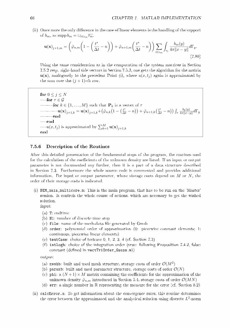
66 CHAPTER 7. MATLAB IMPLEMENTATION
(ii) Once more the only dierence in the case of linear elements is the handling of the supportof bm, as supp bm = ∪i∈ιmτm.
u(x)j+1,m =
(ϕn,m
(1−
(t∗
∆t− n
))+ ϕn+1,m
(t∗
∆t− n
))∑i∈ιm
∫τi
bm(y)
4π‖x− y‖dΓy.
(7.80)
Using the same consideration as in the computation of the system matrices in Section7.5.2 resp. right-hand side vectors in Section 7.5.3, one gets the algorithm for the matrixu(x), analogously to the precedent Point (i), where u(x, tj) again is approximated bythe sum over the (j + 1)-th row.
for 0 ≤ j ≤ N for τ ∈ G for k ∈ 1, . . . ,M such that Pk is a vertex of τ
u(x)j+1,k = u(x)j+1,k+(ϕn,k
(1−
(t∗
∆t − n))
+ ϕn+1,k
(t∗
∆t − n)) ∫
τbk(y)
4π‖x−y‖dΓy end
end
u(x, tj) is approximated by∑M
k=1 u(x)j+1,k
end
7.5.6 Description of the Routines
After this detailed presentation of the fundamental steps of the program, the routines usedfor the calculation of the coecients of the unknown density are listed. If an input or outputparameter is not documented any further, then it is a part of a data structure describedin Section 7.3. Furthermore the whole source code is commented and provides additionalinformation. For input or output parameter, whose storage costs depend on M or N , theorder of their storage costs is indicated.
(i) BEM_main_multicore.m: This is the main program, that has to be run on the 'Master'session. It controls the whole course of actions, which are necessary to get the wishedsolution.input:
(a) T: endtime(b) N1: number of discrete time step(c) file: name of the mesh-data le generated by Gmsh(d) order: polynomial order of approximation (0: piecewise constant elements; 1:
continuous, piecewise linear elements)(e) testCase: choice of testcase 0, 1, 2, 3, 4 (cf. Section 7.3)(f) intlogh: choice of the integration order (true: following Proposition 7.4.2, false:
constant (dened in vectTriOrder_Gauss.m))
output:
(a) meshb: built and used mesh structure, storage costs of order O(M2)(b) paramb: built and used parameter structure, storage costs of order O(N)(c) phi: a (N + 1)×M matrix containing the coecients for the approximation of the
unknown density ϕn,m introduced in Section 5.4, storage costs of order O(MN)(d) err: a single number in R representing the measure for the error (cf. Section 8.2)
(ii) calcError.m: To get information about the convergence rates, this routine determinesthe error between the approximated and the analytical solution using discrete L2-norm
7.5. ROUTINES 67
of Section 8.2.input:
(a) sol: a (N + 1) × Nτ matrix with the values of the analytical solution at themidpoints of the triangle, storage costs of order O(MN)
(b) phi: cf. description of BEM_main_multicore.m, storage costs of order O(MN)
output:
(a) err: cf. description of BEM_main_multicore.m
(iii) completeMeshData.m: To get all the information which are saved in the mesh structure,this routine does all the needed computations. Some part are taken or inspired by thepackage MESH2D by Darren Engwirda3. Especially the routine connectivity.m wasvery helpful.input: noneoutput: none
(iv) getRightSide.m: This routine calculates the right-hand side vector gl for each 0 ≤ l ≤N as introduced in equation (5.56). It works for right-hand side functions g(x, t) (justpass one argument) as well as for right-hand side functions of tensor form g(t)e(x)input:
(a) g: a function handle for g(x, t) resp. the time dependent part g(t)(b) e: a function handle for the space dependent part e(x)
output: b: a M × (N + 1) matrix containing the vector gl in the l-th column, storagecosts of order O(MN)
(v) getSolution.m: In dierent test cases (0 and 1), it is possible to calculate the analyticalsolution. This routine determines the value of the analytical solution at the midpointsof the triangles at all dierent time steps.input:
(a) dg: a function handle for the derivative of time dependent part written as g′(t)(b) e: a function handle for the space dependent part e(x)
output:
(a) sol: a (N + 1) × Nτ matrix with the values of the analytical solution at themidpoints of the triangle, storage costs of order O(MN)
(vi) getSystemMatrix.m: This routine calculates the system matrix for one Helmholtz prob-lem using the formula in equation (5.55) and the 'Quadrature' package. Further detailson the structure of this routine is provided at the end of the Section 7.4.input:
(a) t: a single natural number giving the index of the time step 0 ≤ t ≤ Noutput:
(a) A: a M ×M matrix representing the system matrix, storage costs of order O(M2)
(vii) IFFTlambda.m: To calculate the coecients of the unknown density ϕ for the waveequation out of the coecients ϕ for the dierent Helmholtz problems, this routineimplements the formula (5.57) in vectorized form.input:
(a) phihat: a (N + 1)×M matrix containing the coecients of the unknown densitiesϕn,m for the Helmholtz problems given by (5.56), storage costs of order O(MN)
3The package can be found on the homepage of MATLAB Central http://www.mathworks.com/
matlabcentral/fileexchange/25555-mesh2d-automatic-mesh-generation (13.10.2010)
68 CHAPTER 7. MATLAB IMPLEMENTATION
output:
(a) phi: a (N + 1)×M matrix containing the coecients for the approximation of theunknown density ϕn,m for the Equations (5.44), storage costs of order O(MN)
(viii) readMeshFile.m: This is the routine that reads the .msh-le generated by Gmsh andlls the data into the mesh structure.input:
(a) filename: a string containing the name of the .msh-le
output: none
(ix) solveTimeStep.m: This is the main routine that handles the solving of a a singleHelmholtz problem in the dierent MATLAB sessions. The arising system of linearequations is solved using the built-in function linsolve, that uses an LU factorization.input:
(a) l: a single natural number giving the index of the time step 0 ≤ l ≤ N(b) b: a M × 1 vector representing the right-hand side vector for the l-th Helmholtz
problem, storage costs of order O(M)
output:
(a) phihat: a (N + 1)×M matrix containing the coecients of the unknown densitiesϕn,m for the Helmholtz problems given by (5.56), storage costs of order O(MN)
(x) vectTriOrder_Gauss.m: This routine generates vectorized integration data prepared forthe 'Quadrature'-package and determines the needed integration order using the rulespresented in Table 7.1.input:
(a) order: the polynomial order of approximation dening the used boundary elementfunctions
output: none
To calculate the coecients of the right-hand side vectors and the system matrices, a 'Quadra-ture' package is employed. That package was developed by Dursun Akay (cf. [Aka10]) incollaboration with the author. It consists of the following les:
evalInt.m, GauLeg.mat, gaussQuad.m, gaussQuad_X_W.m, gaussQuadMain.m,gaussQuadMainPlot.m, gaussQuadStep.m, getIndexMat.m, getJacobian.m,
getTriangleMat.m, getTriangleVertices.m, getVariable.m, k3.m, linTransform.m
Not all of them are described any further, as in the nal implementation optimized and morespecic versions of several routines are applied.
Let us describe the optimized functions in more detail, however we skip the input and outputarguments. They are structured into several sections. The rst one is executed during thepreprocessing phase by calling the le 'getVariableOnce.m'.
(i) GauLeg.mat: A list containing high precision weights and nodes for Gauss quadratureon [0, 1] up to the order 100.
(ii) gaussQuad_X_W.m: Here the integration nodes and weights are loaded from GauLeg.mat
for given integration order.
(iii) getIndexMat.m: That is a routine providing a special matrix of indices.
7.5. ROUTINES 69
(iv) getOptIndex.m: This routine loads and provides the information about the occurringintegration weights and nodes.
(v) getTriangleMat.m: Herein the matrices for the ane transformations χτ for a wholeset of triangles G are built.
(vi) getVariableOnce.m: This is the main routine for the preparation of the integration pro-cess. It gets all prepared data from the main program and provides the data concerningthe integration to solve the dierent Helmholtz problems.
The second part contains the routines for calculating the right-hand side vectors using thealgorithms developed in Section 7.5.3.
(i) gaussQuadMain_2d.m: That is the main routine handling the integration of the form∫τ · · · .
(ii) k3_2d.m: Here the integrand is evaluated at the chosen nodes and then multiplied bythe basis functions.
(iii) linTransform.m: In that routine the nodes are projected onto the occurring triangle τusing χτ .
In the third and last part, the routines for the quadrature used for calculating the systemmatrices following the algorithms of Section 7.5.2 are listed.
(i) evalComEdge.m: Herein the quadrature in the case of common edges is handled.
(ii) evalComVert.m: Herein the quadrature in the case of common vertices or distant trian-gles is handled.
(iii) evalIdentical.m: Herein the quadrature in the case of identical triangles is handled.
(iv) gaussQuadMain_4d.m: That is the main routine to handle the quadrature of integrals ofthe form
∫τ
∫t · · · .
(v) k3_4d.m: Here the integrand is evaluated at the chosen nodes and then multiplied bythe basis functions.
(vi) linTransform.m: In that routine the nodes are projected onto the occurring triangle τusing χτ .
Finally a description of the les for the calculation of the solution of the wave equation ufollows. For the calculation of the values, there is no restriction for the chosen eld pointsx ∈ Ω. However, the points have to be arranged properly in a single plane in order to get aplot of the cross section of the wave.
(i) calcWaveFunction_multicore.m: This routine handles the calculation of the solutionof the wave equation. It distributes the work on arbitrary many MATLAB session as itis known from BEM_main_multicore.m. In the source code, the eld points, where thewave function shall be calculated, are dened.input:
(a) phi: the coecients for the unknown density ϕ resulted from BEM_main_multicore.m
(b) mesht: the corresponding mesh structure(c) paramt: the corresponding param structure
output:
70 CHAPTER 7. MATLAB IMPLEMENTATION
(a) u: the value of the solution of the wave equation u at the equidistant discretetimesteps and the above chosen points
(b) film: the resulting lm generated by MATLAB for the use in the function movie
(c) graphb: a structure containing all information about the chosen eld points in theouter space
(ii) gaussQuadMain_Wave.m: That is the routine executing the integration over one triangleτ in the algorithms developed in Section 7.5.5.
(iii) generateGraphicPoints.m: This routine creates all information about the eld points.input: noneoutput: none
(iv) plotWaveFunction.m: This function generates the plots for the dierent timesteps andmerges them together into a lm.input:
(a) u: the discrete values of the wave function(b) graph: cf. description of calcWaveFunction_multicore.m
output:
(a) film: cf. description of calcWaveFunction_multicore.m
To evaluate the solution of the wave equation in a cuboid and present it in a more 3D-stylethere are functions with the sux _slice, which currently are not parallelized. Furthermorethere are a few functions to complete the whole package. They allow solving the problem P(cf. Equation (2.4)) for a given incoming wave on R3 and plotting then the total wave utot.That allows the full animation of the scattering of a certain wave at an obstacle.
(i) calcTotalWave.m: This routine adds the value of the incoming wave to the value of thescattered wave at the eld points.input:
(a) u: a result of calcWaveFunction_multicore.m(b) param: a result of BEM_main_multicore.m(c) graph: a result of calcWaveFunction_multicore.m
output:
(a) u: the sum of the values of the incoming and scattered wave at the eld points
(ii) plotWaveFunction_total.m: That is the nal routine generating the lm of the totalwave including the scatterer.input:
(a) u: a result of calcTotalWave.m(b) graph: a result of calcWaveFunction_multicore.m(c) mesh: a result of BEM_main_multicore.m
output:
(a) film: cf. description of calcWaveFunction_multicore.m
The program ow for calculating the total wave, that is caused by the scattering of an incomingwave at a scatterer, is listed in Figure 7.5.
7.6. STORAGE COSTS 71
compute the coefficients of the unknown densityBEM main multicore.m
compute the scattered wave at defined pointscalcWaveFunction multicore.m
add the incoming wavecalcTotalWave.m
generate a film showing the scatterer and the total waveplotWaveFunction total.m
Figure 7.5: Schematic application ow of the entire package
For the two main routines with a sux _multicore, there exist also the same les without thatsux. These are the routines which do not use the 'Multicore' package and solve everythingon one MATLAB session. However, they use the same routines as the parallelized versions.
Furthermore, a testdriver is provided with the le testDriver.m allowing to do tests forvarious M and N . It is used together with the terminal script startBEMCluster that isable to start several MATLAB sessions as well as the main routines for the calculation ofthe unknown density. For that reason, the main les of the 'Multicore' package are slightlymodied. The documentation can be found in the source code of the les as comments.Further les, also commented, used for such tests are
startBEMMaster.m, startBEMSlave.m, startmulticoreslaveBEM.m,startmulticoremasterBEM.m.
7.6 Storage Costs
After having introduced the necessary global data structure in Section 7.3, input and outputarguments of the routines in Section 7.5 and the data structure for the quadrature package inSection 7.5.1 we discuss the storage costs of the whole implementation. The following orderof storage costs appear in the implementation, focusing on the data structures and not ontheir eld variables:
(i) O(M2): This order arises as storage costs of the structure mesh, the system matricesAl and structure quadrature providing the information for the quadrature package (cf.Section 7.5.1).
(ii) O(MN): Any matrix containing the coecients ϕl,m or ϕl,m, the matrix containing allthe right-hand side vectors gl for all decoupled systems as well as storing the value ofthe analytical solution in all barycenter for all times uses storage of the order O(MN).
(iii) O(N): The structure param only depends linearly on N .
−→ Overall that results in storage costs for the whole implementation on a sequential com-puter of the order
O(MN) +O(M2). (7.81)
In contrast to the storage costs of order O(M2N) for solving the block Toeplitz systemin (5.34) arising in the direct approach, our approach provides a major improvement withrespect to the storage costs at the expense of solving N systems of linear equations. As theseN systems of linear equations are independent, they can be solved on a parallel computer.
72 CHAPTER 7. MATLAB IMPLEMENTATION
Assuming that P processors are available, the distributed memory requirement increases toO(PM2) whereas the needed time is reduced by the factor P . In our tests a typical choice isP = 6.
For the nal time T applied in this thesis, N is much smaller than M , as it can be seen inthe parameters chosen for the tests in Section 8.3. According to the choice ∆t2 ∼ hm+3/2 and
taking into account that ∆t ∼ 1N respectively h ∼ 1√
M, a typical choice is M ∼ N
82m+3 . As
8 > 2m + 3 for m ∈ 0, 1, the order of the storage costs observed during the tests behavesas O(M2), which dominates the order O(MN).
The philosophy to prepare in a preprocessing phase all necessary information, e.g. about themesh or the arranged integration domains, causes the need to store this information in datastructures. To apply the quadrature in its current, vectorized version further information,concerning the integration order or the parametrization of the triangles, has to be providedand is necessary to be stored. As the information for the quadrature routine scale with O(M2)various matrices in the structure quadrature, which also need the same order of storage, arekept in memory without being used after the preprocessing phase, as they do not change theoverall order of the storage costs. However, they provide useful information about the meshwhich simplies the debugging of the code.

Chapter 8
Numerical Tests
All numerical tests using the presented implementation are run on a parallel computer, called'Baxter', built of 64 processors (Intel Xeon X7550) and equipped with approximately 500gigabyte RAM. As the computer also is in use for other projects, at the most 20 and normallyabout 7 MATLAB sessions were started at the same time.
8.1 Test Case with known Analytical Solution
To validate the MATLAB program, we need a right-hand side function g, where the analyticalsolution ϕ of V ϕ = g is known explicitly. Therefore, we take data g separable in time andspace. Let us use the notation
g(t, x) = g(t)e(x). (8.1)
As scatterer we choose the unit sphere S2 in R3. For e(x) we use an eigenfunction of V . Theseare the spherical harmonics Y m
l (θ, ϕ), which are introduced in Section 3.8. As test case, wechoose the spherical harmonic for l = m = 1. In spherical coordinates it holds
Y 11 (θ, ϕ) = −
√3
8πsin(θ)eiϕ. (8.2)
We set as e(x) the spherical harmonic Y 11 in Cartesian coordinates. In [SV11] it is shown,
that for t ∈ [0, 2) the density ϕ solving the problem (2.8) is given by
ϕ(t, x) =
(2g′(t) + 2
∫ t
0sinh(τ)g′(t− τ)dτ
)· e(x). (8.3)
For t ≥ 2 there also exists a formula for the exact solution ϕ. However it is not implemented,as several integrals have to be evaluated. Similar results concerning the choice e(x) = Y 0
0 (x)are presented in [ibid.] as well, where the formula for t > 0 is much simpler, whereas this testcase also is implemented. However, as Y 0
0 = 12√πis constant, there is no dependence with
respect to x. That is the reason why this test case does not appear in any convergence test.
8.2 Error Measure
The result of Theorem 6.3.3 shows that we have to measure the error for each timesteptn, 0 ≤ n ≤ N in the H−1/2(Γ)-norm. As this norm is very time consuming to be evaluatednumerically, we assume higher smoothness of ϕ and measure the error in a discrete L2(Γ)-norm. The arising integral over Γ is split into a sum of integrals over a single panel τ . Theapproximation of the error then is done one these single panels τ . Therefore, the dierence at
73
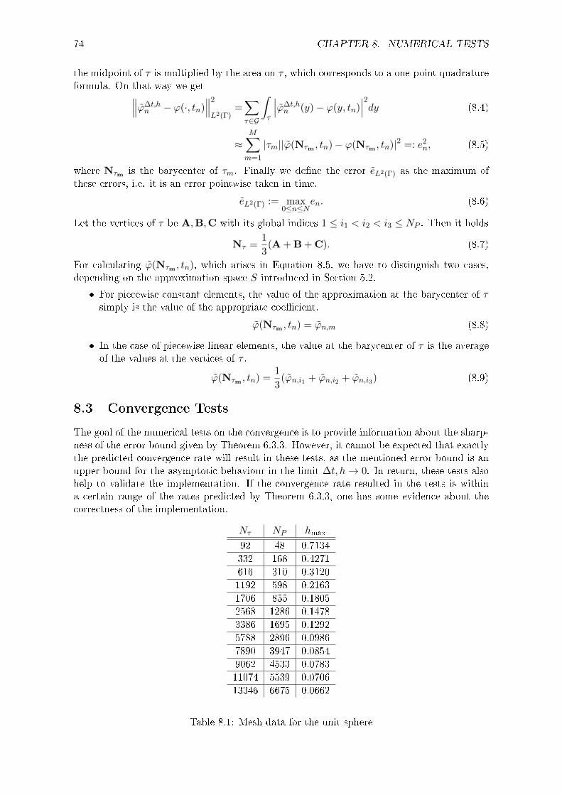
74 CHAPTER 8. NUMERICAL TESTS
the midpoint of τ is multiplied by the area on τ , which corresponds to a one-point quadratureformula. On that way we get∥∥∥ϕ∆t,h
n − ϕ(·, tn)∥∥∥2
L2(Γ)=∑τ∈G
∫τ
∣∣∣ϕ∆t,hn (y)− ϕ(y, tn)
∣∣∣2dy (8.4)
≈M∑m=1
|τm||ϕ(Nτm , tn)− ϕ(Nτm , tn)|2 =: e2n, (8.5)
where Nτm is the barycenter of τm. Finally we dene the error eL2(Γ) as the maximum ofthese errors, i.e. it is an error pointwise taken in time.
eL2(Γ) := max0≤n≤N
en. (8.6)
Let the vertices of τ be A,B,C with its global indices 1 ≤ i1 < i2 < i3 ≤ NP . Then it holds
Nτ =1
3(A + B + C). (8.7)
For calculating ϕ(Nτm , tn), which arises in Equation 8.5, we have to distinguish two cases,depending on the approximation space S introduced in Section 5.2.
For piecewise constant elements, the value of the approximation at the barycenter of τsimply is the value of the appropriate coecient.
ϕ(Nτm , tn) = ϕn,m (8.8)
In the case of piecewise linear elements, the value at the barycenter of τ is the averageof the values at the vertices of τ .
ϕ(Nτm , tn) =1
3(ϕn,i1 + ϕn,i2 + ϕn,i3) (8.9)
8.3 Convergence Tests
The goal of the numerical tests on the convergence is to provide information about the sharp-ness of the error bound given by Theorem 6.3.3. However, it cannot be expected that exactlythe predicted convergence rate will result in these tests, as the mentioned error bound is anupper bound for the asymptotic behaviour in the limit ∆t, h→ 0. In return, these tests alsohelp to validate the implementation. If the convergence rate resulted in the tests is withina certain range of the rates predicted by Theorem 6.3.3, one has some evidence about thecorrectness of the implementation.
Nτ NP hmax
92 48 0.7134
332 168 0.4271
616 310 0.3120
1192 598 0.2163
1706 855 0.1805
2568 1286 0.1478
3386 1695 0.1292
5788 2896 0.0986
7890 3947 0.0854
9062 4533 0.0783
11074 5539 0.0706
13346 6675 0.0662
Table 8.1: Mesh data for the unit sphere
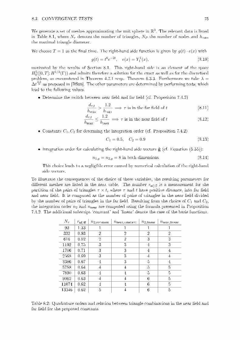
8.3. CONVERGENCE TESTS 75
We generate a set of meshes approximating the unit sphere in R3. The relevant data is listedin Table 8.1, where Nτ denotes the number of triangles, NP the number of nodes and hmax
the maximal triangle diameter.
We choose T = 1 as the nal time. The right-hand side function is given by g(t) · e(x) with
g(t) = t6e−2t, e(x) = Y 11 (x), (8.10)
motivated by the results of Section 8.1. This right-hand side is an element of the spaceH5
0 ([0, T ];H1/2(Γ)) and admits therefore a solution for the exact as well as for the discretisedproblem, as encountered in Theorem 4.7.1 resp. Theorem 6.3.3. Furthermore we take λ =∆t
2.5N as proposed in [BS08]. The other parameters are determined by performing tests, which
lead to the following values.
Determine the switch between near eld and far eld (cf. Proposition 7.4.2)
dτ,thmax
>1.2
hmax=⇒ τ is in the far eld of t (8.11)
dτ,thmax
≤ 1.2
hmax=⇒ τ is in the near eld of t (8.12)
Constants C1, C2 for determing the integration order (cf. Proposition 7.4.2)
C1 = 0.5, C2 = 0.9 (8.13)
Integration order for calculating the right-hand side vectors g (cf. Equation (5.55)):
n1,g = n2,g = 8 in both dimensions (8.14)
This choice leads to a negligible error caused by numerical calculation of the right-handside vectors.
To illustrate the consequences of the choice of these variables, the resulting parameters fordierent meshes are listed in the next table. The number rnf/ is a measurement for thepartition of the pairs of triangles τ × t, where τ and t have positive distance, into far eldand near eld. It is computed as the number of pairs of triangles in the near eld dividedby the number of pairs of triangles in the far eld. Resulting from the choice of C1 and C2,the integration order n2 and nnear are computed using the formula presented in Proposition7.4.2. The additional subscript 'constant' and 'linear' denote the case of the basis functions.
Nτ rnf/ n2,constant nnear,constant n2,linear nnear,linear
92 1.33 1 1 1 1
332 0.93 2 2 2 2
616 0.82 2 2 3 3
1192 0.75 3 3 4 3
1706 0.71 3 3 4 4
2568 0.69 3 3 4 4
3386 0.67 4 3 5 4
5788 0.64 4 4 5 5
7890 0.63 4 4 5 5
9062 0.63 4 4 6 5
11074 0.62 4 4 6 5
13346 0.62 5 4 6 5
Table 8.2: Quadrature orders and relation between triangle combinations in the near eld andfar eld for the proposed constants
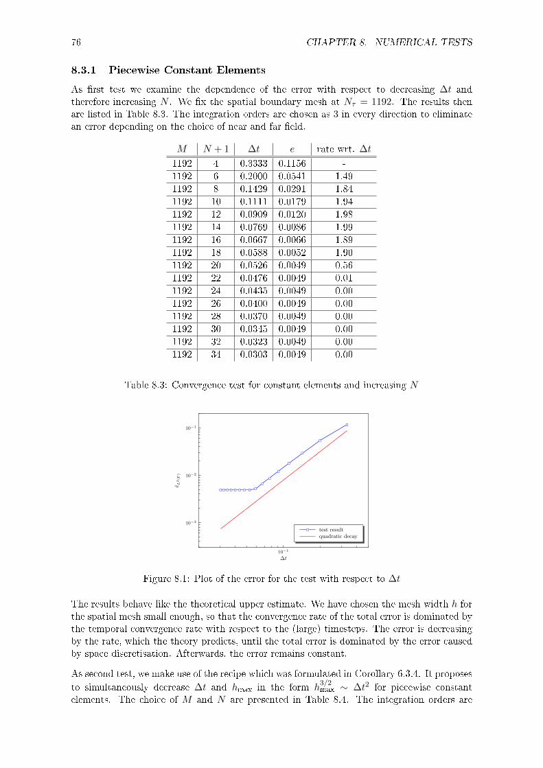
76 CHAPTER 8. NUMERICAL TESTS
8.3.1 Piecewise Constant Elements
As rst test we examine the dependence of the error with respect to decreasing ∆t andtherefore increasing N . We x the spatial boundary mesh at Nτ = 1192. The results thenare listed in Table 8.3. The integration orders are chosen as 3 in every direction to eliminatean error depending on the choice of near and far eld.
M N + 1 ∆t e rate wrt. ∆t
1192 4 0.3333 0.1156 -
1192 6 0.2000 0.0541 1.49
1192 8 0.1429 0.0291 1.84
1192 10 0.1111 0.0179 1.94
1192 12 0.0909 0.0120 1.98
1192 14 0.0769 0.0086 1.99
1192 16 0.0667 0.0066 1.89
1192 18 0.0588 0.0052 1.90
1192 20 0.0526 0.0049 0.56
1192 22 0.0476 0.0049 0.01
1192 24 0.0435 0.0049 0.00
1192 26 0.0400 0.0049 0.00
1192 28 0.0370 0.0049 0.00
1192 30 0.0345 0.0049 0.00
1192 32 0.0323 0.0049 0.00
1192 34 0.0303 0.0049 0.00
Table 8.3: Convergence test for constant elements and increasing N
10−1
10−3
10−2
10−1
∆t
eL
2(Γ
)
rS
rS
rS
rS
rS
rS
rS
rSrSrSrSrSrSrSrSrS
test result
quadratic decay
rS
Figure 8.1: Plot of the error for the test with respect to ∆t
The results behave like the theoretical upper estimate. We have chosen the mesh width h forthe spatial mesh small enough, so that the convergence rate of the total error is dominated bythe temporal convergence rate with respect to the (large) timesteps. The error is decreasingby the rate, which the theory predicts, until the total error is dominated by the error causedby space discretisation. Afterwards, the error remains constant.
As second test, we make use of the recipe which was formulated in Corollary 6.3.4. It proposes
to simultaneously decrease ∆t and hmax in the form h3/2max ∼ ∆t2 for piecewise constant
elements. The choice of M and N are presented in Table 8.4. The integration orders are
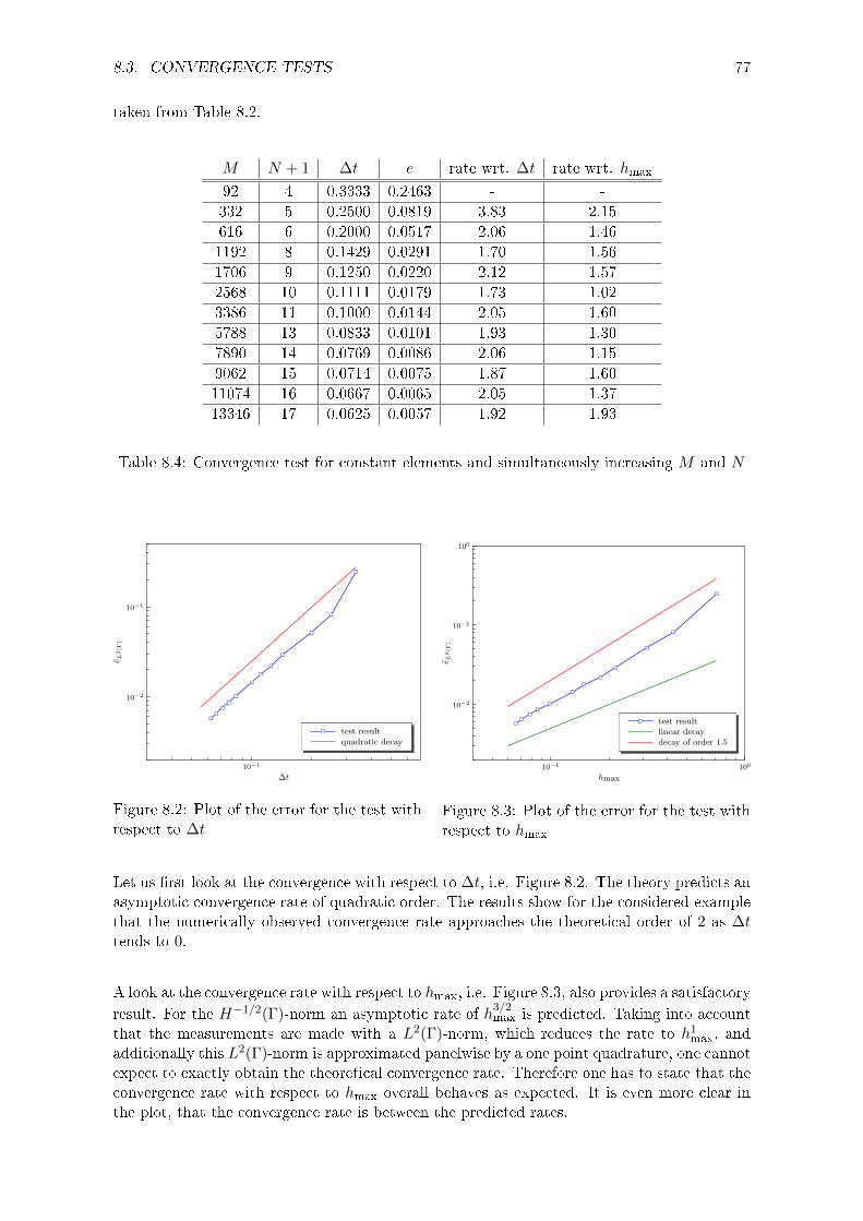
8.3. CONVERGENCE TESTS 77
taken from Table 8.2.
M N + 1 ∆t e rate wrt. ∆t rate wrt. hmax
92 4 0.3333 0.2463 - -
332 5 0.2500 0.0819 3.83 2.15
616 6 0.2000 0.0517 2.06 1.46
1192 8 0.1429 0.0291 1.70 1.56
1706 9 0.1250 0.0220 2.12 1.57
2568 10 0.1111 0.0179 1.73 1.02
3386 11 0.1000 0.0144 2.05 1.60
5788 13 0.0833 0.0101 1.93 1.30
7890 14 0.0769 0.0086 2.06 1.15
9062 15 0.0714 0.0075 1.87 1.60
11074 16 0.0667 0.0065 2.05 1.37
13346 17 0.0625 0.0057 1.92 1.93
Table 8.4: Convergence test for constant elements and simultaneously increasing M and N
10−1
10−2
10−1
∆t
eL
2(Γ
)
rS
rS
rS
rS
rS
rS
rS
rSrS
rSrS
rS
test result
quadratic decay
rS
Figure 8.2: Plot of the error for the test withrespect to ∆t
10−1
100
10−2
10−1
100
hmax
eL
2(Γ
)
rS
rS
rS
rS
rSrS
rS
rSrS
rSrS
rS test result
linear decay
decay of order 1.5
rS
Figure 8.3: Plot of the error for the test withrespect to hmax
Let us rst look at the convergence with respect to ∆t, i.e. Figure 8.2. The theory predicts anasymptotic convergence rate of quadratic order. The results show for the considered examplethat the numerically observed convergence rate approaches the theoretical order of 2 as ∆ttends to 0.
A look at the convergence rate with respect to hmax, i.e. Figure 8.3, also provides a satisfactory
result. For the H−1/2(Γ)-norm an asymptotic rate of h3/2max is predicted. Taking into account
that the measurements are made with a L2(Γ)-norm, which reduces the rate to h1max, and
additionally this L2(Γ)-norm is approximated panelwise by a one point quadrature, one cannotexpect to exactly obtain the theoretical convergence rate. Therefore one has to state that theconvergence rate with respect to hmax overall behaves as expected. It is even more clear inthe plot, that the convergence rate is between the predicted rates.
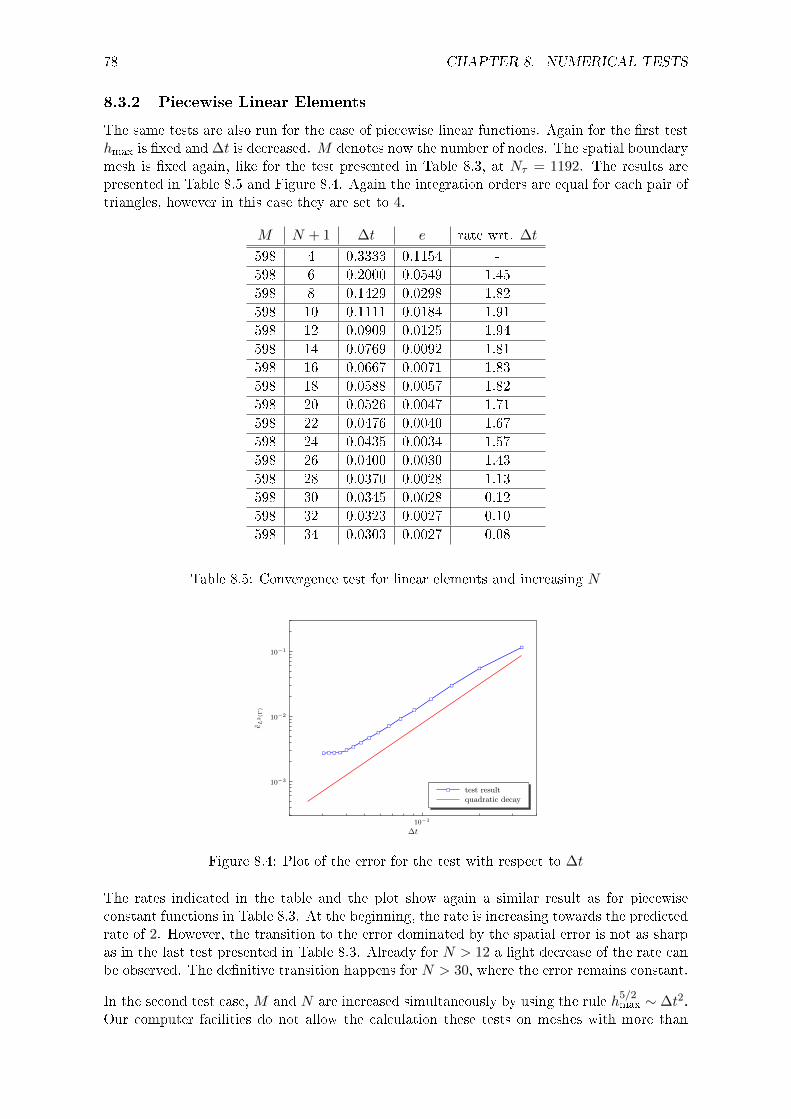
78 CHAPTER 8. NUMERICAL TESTS
8.3.2 Piecewise Linear Elements
The same tests are also run for the case of piecewise linear functions. Again for the rst testhmax is xed and ∆t is decreased. M denotes now the number of nodes. The spatial boundarymesh is xed again, like for the test presented in Table 8.3, at Nτ = 1192. The results arepresented in Table 8.5 and Figure 8.4. Again the integration orders are equal for each pair oftriangles, however in this case they are set to 4.
M N + 1 ∆t e rate wrt. ∆t
598 4 0.3333 0.1154 -
598 6 0.2000 0.0549 1.45
598 8 0.1429 0.0298 1.82
598 10 0.1111 0.0184 1.91
598 12 0.0909 0.0125 1.94
598 14 0.0769 0.0092 1.81
598 16 0.0667 0.0071 1.83
598 18 0.0588 0.0057 1.82
598 20 0.0526 0.0047 1.71
598 22 0.0476 0.0040 1.67
598 24 0.0435 0.0034 1.57
598 26 0.0400 0.0030 1.43
598 28 0.0370 0.0028 1.13
598 30 0.0345 0.0028 0.12
598 32 0.0323 0.0027 0.10
598 34 0.0303 0.0027 0.08
Table 8.5: Convergence test for linear elements and increasing N
10−1
10−3
10−2
10−1
∆t
eL
2(Γ
)
rS
rS
rS
rS
rS
rS
rSrS
rSrS
rSrSrSrSrSrS
test result
quadratic decay
rS
Figure 8.4: Plot of the error for the test with respect to ∆t
The rates indicated in the table and the plot show again a similar result as for piecewiseconstant functions in Table 8.3. At the beginning, the rate is increasing towards the predictedrate of 2. However, the transition to the error dominated by the spatial error is not as sharpas in the last test presented in Table 8.3. Already for N > 12 a light decrease of the rate canbe observed. The denitive transition happens for N > 30, where the error remains constant.
In the second test case, M and N are increased simultaneously by using the rule h5/2max ∼ ∆t2.
Our computer facilities do not allow the calculation these tests on meshes with more than

8.4. COMPLEXITY TESTS 79
8000 triangles in a reasonable time. Therefore the maximal mesh contains 7890 triangles,for which the solving of one single Helmholtz problem takes 10 hours. Again the integrationorders are chosen increasingly, like presented in Table 8.2.
M N + 1 ∆t e rate wrt. ∆t rate wrt. hmax
48 3 0.5000 0.3663 - -
168 4 0.3333 0.1142 2.88 2.27
310 5 0.2500 0.0850 1.03 0.94
598 7 0.1667 0.0391 1.91 2.12
855 8 0.1429 0.0296 1.81 1.54
1286 10 0.1111 0.0182 1.95 2.45
1695 12 0.0909 0.0122 1.98 2.95
2896 16 0.0667 0.0066 1.97 2.26
3947 19 0.0556 0.0046 2.00 2.53
Table 8.6: Convergence test for linear elements and simultaneously increasing M and N
10−1
10−2
10−1
∆t
eL
2(Γ
)
rS
rS
rS
rS
rS
rS
rS
rS
rStest result
quadratic decay
rS
Figure 8.5: Plot of the error for the test withrespect to ∆t
10−1
10−2
10−1
100
hmax
eL
2(Γ
)
rS
rS
rS
rS
rS
rS
rS
rS
rS
test result
quadratic decay
decay of order 2.5
rS
Figure 8.6: Plot of the error for the test withrespect to hmax
Again the predicted convergence rate with respect to ∆t is achieved. The rate approaches theasymptotic theoretical order of 2. The error with respect to hmax behaves similarly as in thetest case for piecewise constant elements presented in Table 8.4. The theory predicts a rate
of h5/2max in the H−1/2(Γ)-norm, and therefore h2
max in the L2(Γ) norm. The obtained rates lieoverall in this given range, which the plot also shows.
In summary, the implementation is validated by these test results and there is evidence thatthe theoretical asymptotic convergence rate is sharp.
8.4 Complexity Tests
In this section we will discuss the question of the complexity of the implemented method. AsN + 1 dierent Helmholtz problems are solved and the system matrices have the dimensionM ×M , one expects complexity of O(NM2) due to the fact that no technique for reducingthat complexity is applied in this implementation.
First of all, let us have a look at the time consumption of the various MATLAB routines. The
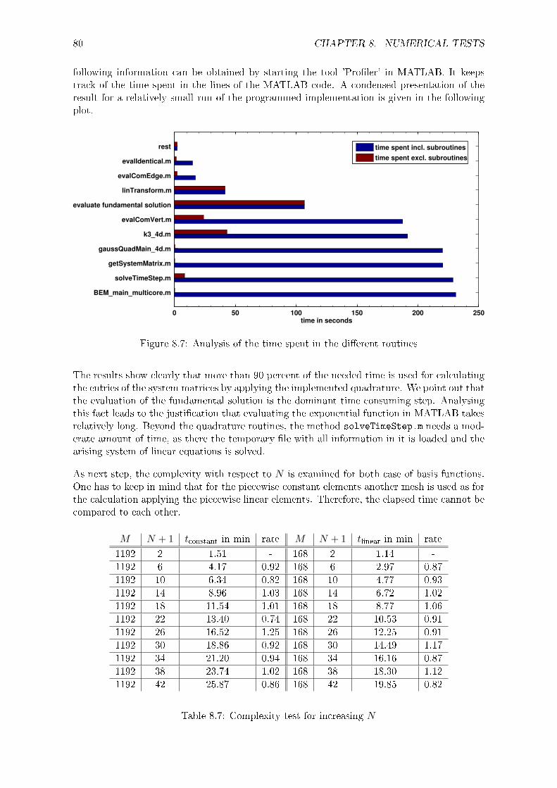
80 CHAPTER 8. NUMERICAL TESTS
following information can be obtained by starting the tool 'Proler' in MATLAB. It keepstrack of the time spent in the lines of the MATLAB code. A condensed presentation of theresult for a relatively small run of the programmed implementation is given in the followingplot.
0 50 100 150 200 250
BEM_main_multicore.m
solveTimeStep.m
getSystemMatrix.m
gaussQuadMain_4d.m
k3_4d.m
evalComVert.m
evaluate fundamental solution
linTransform.m
evalComEdge.m
evalIdentical.m
rest
time in seconds
time spent incl. subroutines
time spent excl. subroutines
Figure 8.7: Analysis of the time spent in the dierent routines
The results show clearly that more than 90 percent of the needed time is used for calculatingthe entries of the system matrices by applying the implemented quadrature. We point out thatthe evaluation of the fundamental solution is the dominant time consuming step. Analysingthis fact leads to the justication that evaluating the exponential function in MATLAB takesrelatively long. Beyond the quadrature routines, the method solveTimeStep.m needs a mod-erate amount of time, as there the temporary le with all information in it is loaded and thearising system of linear equations is solved.
As next step, the complexity with respect to N is examined for both case of basis functions.One has to keep in mind that for the piecewise constant elements another mesh is used as forthe calculation applying the piecewise linear elements. Therefore, the elapsed time cannot becompared to each other.
M N + 1 tconstant in min rate M N + 1 tlinear in min rate
1192 2 1.51 - 168 2 1.14 -
1192 6 4.17 0.92 168 6 2.97 0.87
1192 10 6.34 0.82 168 10 4.77 0.93
1192 14 8.96 1.03 168 14 6.72 1.02
1192 18 11.54 1.01 168 18 8.77 1.06
1192 22 13.40 0.74 168 22 10.53 0.91
1192 26 16.52 1.25 168 26 12.25 0.91
1192 30 18.86 0.92 168 30 14.49 1.17
1192 34 21.20 0.94 168 34 16.16 0.87
1192 38 23.74 1.02 168 38 18.30 1.12
1192 42 25.87 0.86 168 42 19.85 0.82
Table 8.7: Complexity test for increasing N
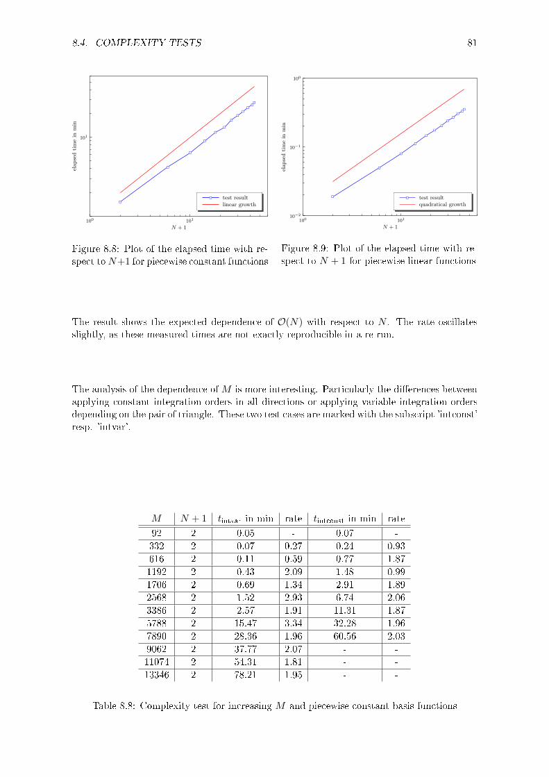
8.4. COMPLEXITY TESTS 81
100
101
101
N + 1
elapsedtimein
min
rS
rS
rS
rS
rS
rS
rSrS
rSrSrSrS
test result
linear growth
rS
Figure 8.8: Plot of the elapsed time with re-spect toN+1 for piecewise constant functions
100
101
10−2
10−1
100
N + 1
elapsedtimein
min
rS
rS
rS
rS
rS
rSrS
rSrSrSrSrS
test result
quadratical growth
rS
Figure 8.9: Plot of the elapsed time with re-spect to N + 1 for piecewise linear functions
The result shows the expected dependence of O(N) with respect to N . The rate oscillatesslightly, as these measured times are not exactly reproducible in a re-run.
The analysis of the dependence ofM is more interesting. Particularly the dierences betweenapplying constant integration orders in all directions or applying variable integration ordersdepending on the pair of triangle. These two test cases are marked with the subscript 'intconst'resp. 'intvar'.
M N + 1 tintvar in min rate tintconst in min rate
92 2 0.05 - 0.07 -
332 2 0.07 0.27 0.24 0.93
616 2 0.11 0.59 0.77 1.87
1192 2 0.43 2.09 1.48 0.99
1706 2 0.69 1.34 2.91 1.89
2568 2 1.52 2.93 6.74 2.06
3386 2 2.57 1.91 11.31 1.87
5788 2 15.47 3.34 32.28 1.96
7890 2 28.36 1.96 60.56 2.03
9062 2 37.77 2.07 - -
11074 2 54.31 1.81 - -
13346 2 78.21 1.95 - -
Table 8.8: Complexity test for increasing M and piecewise constant basis functions
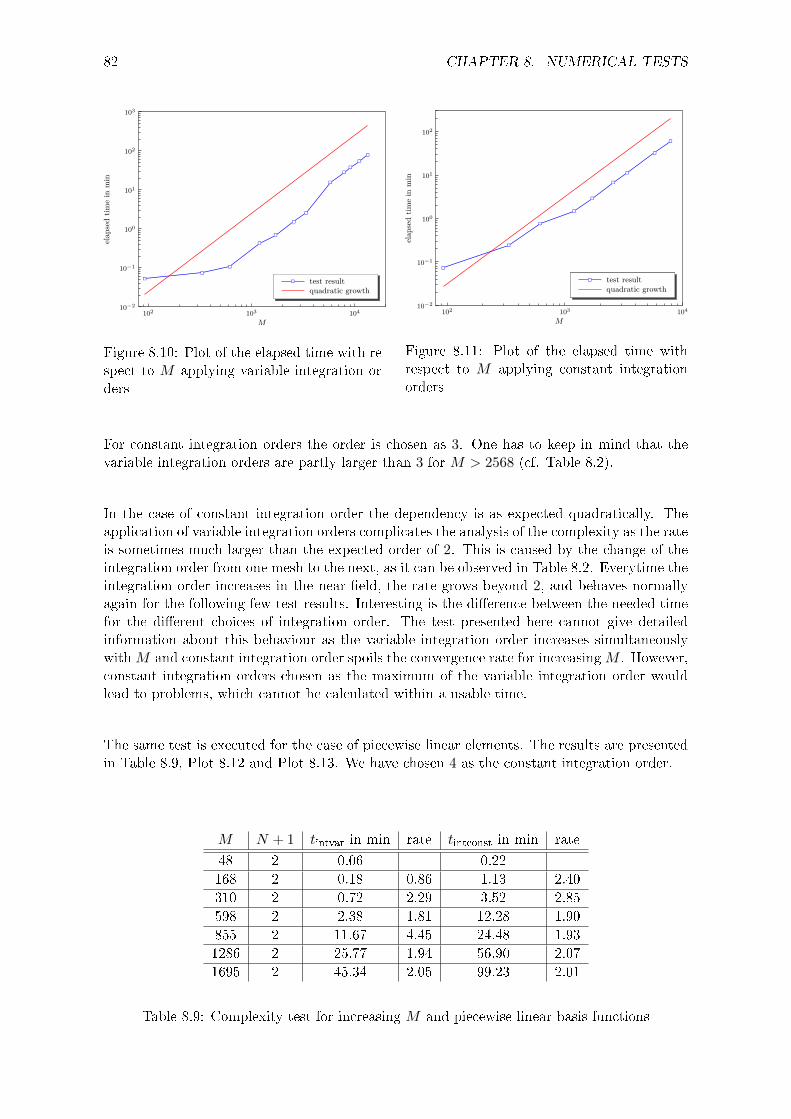
82 CHAPTER 8. NUMERICAL TESTS
102
103
104
10−2
10−1
100
101
102
103
M
elapsedtimein
min
rSrS
rS
rS
rS
rS
rS
rS
rSrS
rSrS
test result
quadratic growth
rS
Figure 8.10: Plot of the elapsed time with re-spect to M applying variable integration or-ders
102
103
104
10−2
10−1
100
101
102
M
elapsedtimein
min
rS
rS
rS
rS
rS
rS
rS
rS
rS
test result
quadratic growth
rS
Figure 8.11: Plot of the elapsed time withrespect to M applying constant integrationorders
For constant integration orders the order is chosen as 3. One has to keep in mind that thevariable integration orders are partly larger than 3 for M > 2568 (cf. Table 8.2).
In the case of constant integration order the dependency is as expected quadratically. Theapplication of variable integration orders complicates the analysis of the complexity as the rateis sometimes much larger than the expected order of 2. This is caused by the change of theintegration order from one mesh to the next, as it can be observed in Table 8.2. Everytime theintegration order increases in the near eld, the rate grows beyond 2, and behaves normallyagain for the following few test results. Interesting is the dierence between the needed timefor the dierent choices of integration order. The test presented here cannot give detailedinformation about this behaviour as the variable integration order increases simultaneouslywithM and constant integration order spoils the convergence rate for increasingM . However,constant integration orders chosen as the maximum of the variable integration order wouldlead to problems, which cannot be calculated within a usable time.
The same test is executed for the case of piecewise linear elements. The results are presentedin Table 8.9, Plot 8.12 and Plot 8.13. We have chosen 4 as the constant integration order.
M N + 1 tintvar in min rate tintconst in min rate
48 2 0.06 - 0.22 -
168 2 0.18 0.86 1.13 2.40
310 2 0.72 2.29 3.52 2.85
598 2 2.38 1.81 12.28 1.90
855 2 11.67 4.45 24.48 1.93
1286 2 25.77 1.94 56.90 2.07
1695 2 45.34 2.05 99.23 2.01
Table 8.9: Complexity test for increasing M and piecewise linear basis functions
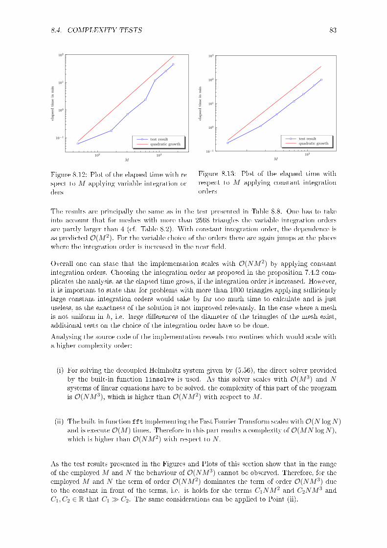
8.4. COMPLEXITY TESTS 83
102
103
10−1
100
101
102
M
elapsedtimein
min
rS
rS
rS
rS
rS
rS
rS
test result
quadratic growth
rS
Figure 8.12: Plot of the elapsed time with re-spect to M applying variable integration or-ders
102
10−1
100
101
102
103
M
elapsedtimein
min
rS
rS
rS
rS
rS
rS
rS
test result
quadratic growth
rS
Figure 8.13: Plot of the elapsed time withrespect to M applying constant integrationorders
The results are principally the same as in the test presented in Table 8.8. One has to takeinto account that for meshes with more than 2568 triangles the variable integration ordersare partly larger than 4 (cf. Table 8.2). With constant integration order, the dependence isas predicted O(M2). For the variable choice of the orders there are again jumps at the placeswhere the integration order is increased in the near eld.
Overall one can state that the implementation scales with O(NM2) by applying constantintegration orders. Choosing the integration order as proposed in the proposition 7.4.2 com-plicates the analysis, as the elapsed time grows, if the integration order is increased. However,it is important to state that for problems with more than 1000 triangles applying sucientlylarge constant integration orders would take by far too much time to calculate and is justuseless, as the exactness of the solution is not improved relevantly. In the case where a meshis not uniform in h, i.e. large dierences of the diameter of the triangles of the mesh exist,additional tests on the choice of the integration order have to be done.
Analysing the source code of the implementation reveals two routines which would scale witha higher complexity order:
(i) For solving the decoupled Helmholtz system given by (5.56), the direct solver providedby the built-in function linsolve is used. As this solver scales with O(M3) and Nsystems of linear equations have to be solved, the complexity of this part of the programis O(NM3), which is higher than O(NM2) with respect to M .
(ii) The built-in function fft implementing the Fast Fourier Transform scales withO(N logN)and is execute O(M) times. Therefore in this part results a complexity of O(MN logN),which is higher than O(NM2) with respect to N .
As the test results presented in the Figures and Plots of this section show that in the rangeof the employed M and N the behaviour of O(NM3) cannot be observed. Therefore, for theemployed M and N the term of order O(NM2) dominates the term of order O(NM3) dueto the constant in front of the terms, i.e. it holds for the terms C1NM
2 and C2NM3 and
C1, C2 ∈ R that C1 C2. The same considerations can be applied to Point (ii).
84 CHAPTER 8. NUMERICAL TESTS
8.5 Acoustic Tests
To check the plausibility of the calculated solution of the wave equation and to perform sometests on the scattering properties of various objects, plane and spherical waves are consideredin the case where the speed of sound is c = 1. Therefore, we go back to the formulation ofthe problem in Chapter 2. As explained there, we consider in Equation (2.2) the case of anincoming wave uinc, that gives us then the right-hand side function g = −uinc on Γ. As theconvergence of the method is proved for the case, where the incoming wave has not reachedthe obstacle at t = 0 and thus g and suciently many of its derivatives are vanishing att = 0, both, the classical spherical as well as the plane wave, are modulated by a Gaussian(see [Ban09]).
Let us look rst at the case of an incoming plane wave. The classical formula for a plane waveis
uinc(x, t) = cos (ω · (t− 〈α, x〉)), (8.15)
where ω ∈ R is the frequency, α ∈ R3 with ‖α‖ = 1 the direction of motion and 〈·, ·〉 theEuclidean scalar product on R3. This is modulated by a Gaussian with parameters for deningthe peak A ∈ R and the speed of decay σ ∈ R. Thus we get the incoming wave
uinc(x, t) := cos (ω · (t− 〈α, x〉)) · exp
(−(t− 〈α, x〉 −A
σ
)2). (8.16)
Let us show, that this function satises the problem Pinc with vanishing inhomogeneity f onthe full space. Therefore, let us introduce the following notation
r := ω · (t− 〈α, x〉), s := −(t− 〈α, x〉 −A
σ
)2
. (8.17)
Using the notation x = (x1, x2, x3)T , α = (α1, α2, α3)T and i ∈ 1, 2, 3, it holds for theirderivatives
rt = ω, rxi = −ωαi, rtt = 0, rxixi = 0, (8.18)
respectively for s
st = −2t− 〈α, x〉 −A
σ2, sxi = 2αi ·
t− 〈α, x〉 −Aσ2
, stt = − 2
σ2, sxixi = −2α2
i
σ2. (8.19)
Therefore we get
(uinc)t =− sin(r) exp(s)rt + cos(r) exp(s)st (8.20)
(uinc)tt =− cos(r) exp(s)r2t − sin(r) exp(s)rtst − sin(r) exp(s)rtt
− sin(r) exp(s)strt + cos(r) exp(s)s2t + cos(r) exp(s)stt (8.21)
= (−r2t + s2
t + stt)︸ ︷︷ ︸a1:=
cos(r) exp(s) + (−2rtst − rtt)︸ ︷︷ ︸a2
sin(r) exp(s), (8.22)
and analogously
(uinc)xi =− sin(r) exp(s)rxi + cos(r) exp(s)sxi (8.23)
(uinc)xixi =(−r2xi + s2
xi + sxixi) cos(r) exp(s) + (−2rxisxi − rxixi) sin(r) exp(s) (8.24)
(∆uinc) =
(3∑i=1
−r2xi + s2
xi + sxixi
)︸ ︷︷ ︸
b1
cos(r) exp(s) +
(3∑i=1
−2rxisxi − rxixi
)︸ ︷︷ ︸
b2
sin(r) exp(s).
(8.25)
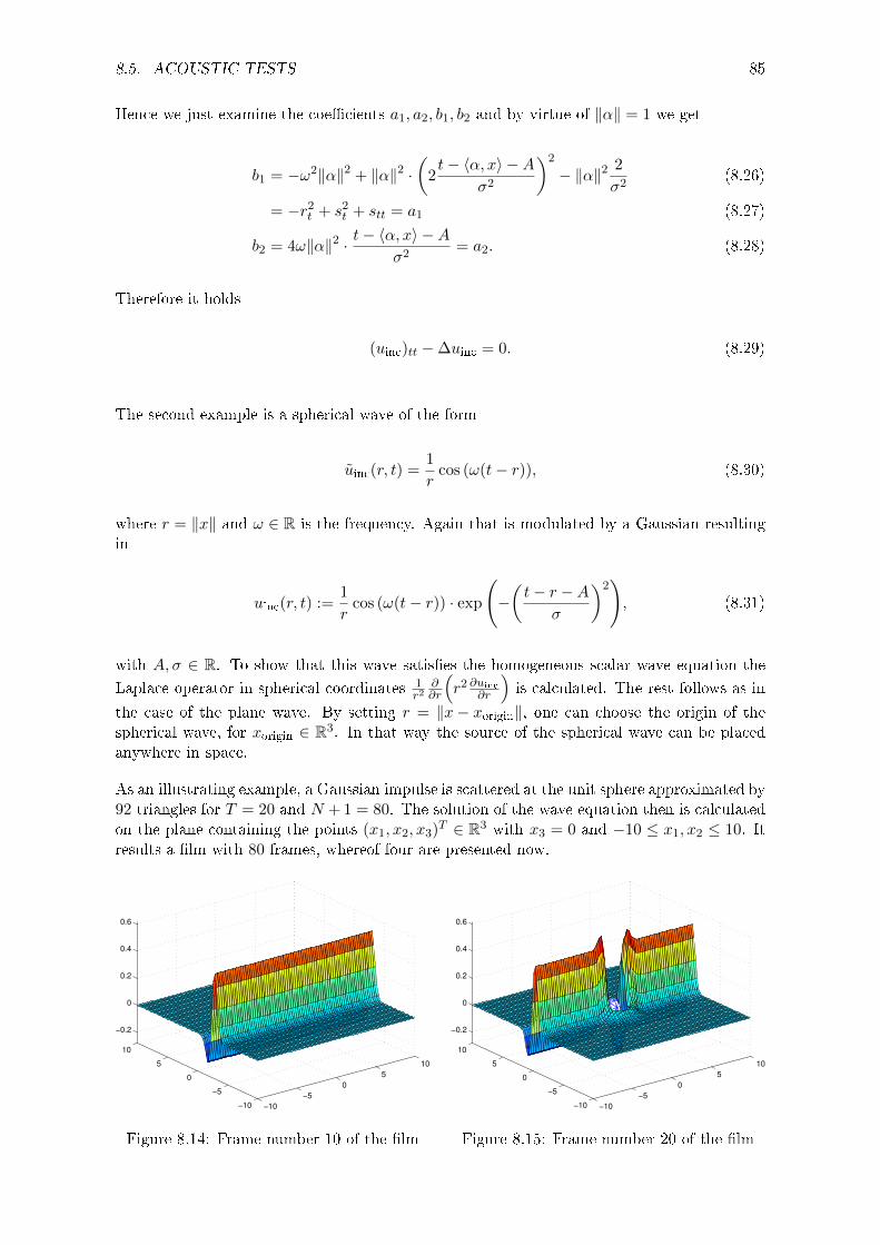
8.5. ACOUSTIC TESTS 85
Hence we just examine the coecients a1, a2, b1, b2 and by virtue of ‖α‖ = 1 we get
b1 = −ω2‖α‖2 + ‖α‖2 ·(
2t− 〈α, x〉 −A
σ2
)2
− ‖α‖2 2
σ2(8.26)
= −r2t + s2
t + stt = a1 (8.27)
b2 = 4ω‖α‖2 · t− 〈α, x〉 −Aσ2
= a2. (8.28)
Therefore it holds
(uinc)tt −∆uinc = 0. (8.29)
The second example is a spherical wave of the form
uinc(r, t) =1
rcos (ω(t− r)), (8.30)
where r = ‖x‖ and ω ∈ R is the frequency. Again that is modulated by a Gaussian resultingin
uinc(r, t) :=1
rcos (ω(t− r)) · exp
(−(t− r −A
σ
)2), (8.31)
with A, σ ∈ R. To show that this wave satises the homogeneous scalar wave equation the
Laplace operator in spherical coordinates 1r2
∂∂r
(r2 ∂uinc
∂r
)is calculated. The rest follows as in
the case of the plane wave. By setting r = ‖x− xorigin‖, one can choose the origin of thespherical wave, for xorigin ∈ R3. In that way the source of the spherical wave can be placedanywhere in space.
As an illustrating example, a Gaussian impulse is scattered at the unit sphere approximated by92 triangles for T = 20 and N + 1 = 80. The solution of the wave equation then is calculatedon the plane containing the points (x1, x2, x3)T ∈ R3 with x3 = 0 and −10 ≤ x1, x2 ≤ 10. Itresults a lm with 80 frames, whereof four are presented now.
−10
−5
0
5
10
−10
−5
0
5
10
−0.2
0
0.2
0.4
0.6
Figure 8.14: Frame number 10 of the lm
−10
−5
0
5
10
−10
−5
0
5
10
−0.2
0
0.2
0.4
0.6
Figure 8.15: Frame number 20 of the lm

86 CHAPTER 8. NUMERICAL TESTS
−10
−5
0
5
10
−10
−5
0
5
10
−0.2
0
0.2
0.4
0.6
Figure 8.16: Frame number 30 of the lm
−10
−5
0
5
10
−10
−5
0
5
10
−0.2
0
0.2
0.4
0.6
Figure 8.17: Frame number 50 of the lm
In frame number 10, the Gaussian impulse has not reached the obstacle yet (it is hiddenbeyond the wave), whereas in frame number 20 some parts of the wave are already diracted.In the next picture one sees the reected parts going back and the notch in the impulse thatthe obstacle has caused. Furthermore, a sharp smaller wave follows the impulse in that notch.In frame number 50 one sees the further propagation of the diracted wave. During the thesisother objects, namely a cuboid and a model of the ancient theater of Epidaurus, are used asscatterers. Some of these results are presented on [Hub10], where the lm containing Figures8.14 - 8.17 is available as well.
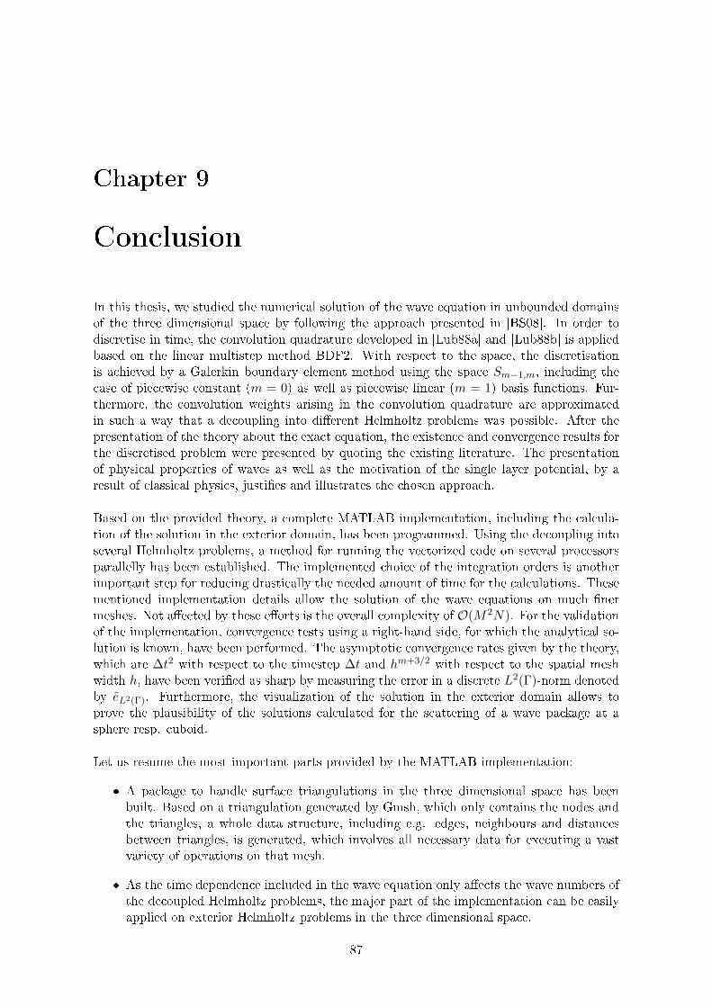
Chapter 9
Conclusion
In this thesis, we studied the numerical solution of the wave equation in unbounded domainsof the three dimensional space by following the approach presented in [BS08]. In order todiscretise in time, the convolution quadrature developed in [Lub88a] and [Lub88b] is appliedbased on the linear multistep method BDF2. With respect to the space, the discretisationis achieved by a Galerkin boundary element method using the space Sm−1,m, including thecase of piecewise constant (m = 0) as well as piecewise linear (m = 1) basis functions. Fur-thermore, the convolution weights arising in the convolution quadrature are approximatedin such a way that a decoupling into dierent Helmholtz problems was possible. After thepresentation of the theory about the exact equation, the existence and convergence results forthe discretised problem were presented by quoting the existing literature. The presentationof physical properties of waves as well as the motivation of the single layer potential, by aresult of classical physics, justies and illustrates the chosen approach.
Based on the provided theory, a complete MATLAB implementation, including the calcula-tion of the solution in the exterior domain, has been programmed. Using the decoupling intoseveral Helmholtz problems, a method for running the vectorized code on several processorsparallelly has been established. The implemented choice of the integration orders is anotherimportant step for reducing drastically the needed amount of time for the calculations. Thesementioned implementation details allow the solution of the wave equations on much nermeshes. Not aected by these eorts is the overall complexity of O(M2N). For the validationof the implementation, convergence tests using a right-hand side, for which the analytical so-lution is known, have been performed. The asymptotic convergence rates given by the theory,which are ∆t2 with respect to the timestep ∆t and hm+3/2 with respect to the spatial meshwidth h, have been veried as sharp by measuring the error in a discrete L2(Γ)-norm denotedby eL2(Γ). Furthermore, the visualization of the solution in the exterior domain allows toprove the plausibility of the solutions calculated for the scattering of a wave package at asphere resp. cuboid.
Let us resume the most important parts provided by the MATLAB implementation:
A package to handle surface triangulations in the three dimensional space has beenbuilt. Based on a triangulation generated by Gmsh, which only contains the nodes andthe triangles, a whole data structure, including e.g. edges, neighbours and distancesbetween triangles, is generated, which involves all necessary data for executing a vastvariety of operations on that mesh.
As the time dependence included in the wave equation only aects the wave numbers ofthe decoupled Helmholtz problems, the major part of the implementation can be easilyapplied on exterior Helmholtz problems in the three dimensional space.
87
88 CHAPTER 9. CONCLUSION
The quadrature package, developed by Dursun Akay and the author, is applicable forany similar integrand tting into the framework presented in [SS04, Chapter 5]. Asquadrature routines are largely decoupled from the other parts of the implementation,there are just few diculties to apply them on other examples. The presented imple-mentation is rather an example for the use of that quadrature package.
The convergence tests provide a rule of thumb for the choice of ∆t and h to attain theoptimal convergence rate by a simultaneous decrease of ∆t and h.
Running the dierent tests on increasingly ner meshes and smaller timesteps revealed thebottlenecks of the current implementation. As mentioned in the discussion of the complexitytests, the evaluation of the exponential function causes a relatively large amount of time.That problem could be reduced by using an approximation of the exponential function, im-plemented in a le in the program language C and included into MATLAB. However there aredierences regarding the limiting factors between the case of piecewise constant and piecewiselinear basis functions. Generally in the case of piecewise constant functions the necessary in-tegration orders are smaller. This allows applying meshes with more than 10'000 triangles,which then needs a temporary le with all informations about the mesh and the integrationexceeding several gigabytes. This amount of needed space could be reduced by changing theintegration package concerning the provided data, as at the moment there is a high redun-dancy caused by the choice of the integration orders. In the application of the piecewise linearbasis functions that problem is dominated by the needed amount of RAM and time. Even withcoarser meshes, a single Helmholtz problem cannot be solved within an appropriate period oftime on the computer facilities which have been available. In addition not many processorscan work parallelly on dierent Helmholtz problems, as the needed amount of RAM wouldeven be too large for the machine 'Baxter', where the tests were run. Some optimizations toreduce these diculties would be possible by revising the quadrature package in combinationwith a stronger linkage to the routine assembling the system matrix.
Furthermore, in [BS08, Chapter 4.2] a possibility for the reduction of the number of Helmholtzproblems is presented for special right-hand side functions g. In order to decrease the overallcomplexity for largerM and N applied in the tests, an iterative solver for the systems of linearequations can be applied. Beside these suggestions for an optimization of the implementationavoiding a fundamental change of the method, there exist possibilities of far-reaching mod-ications to reduce the overall complexity. One possibility is the implementation of a fastmultipole technique or the use of a panel-clustering algorithm for solving a single Helmholtzproblem. In order to reduce storage costs as well one might reorganise the data structuretoo, as in the current implementation the storage costs are of order O(M2) +O(MN). Suchpropositions can be found e.g. in [BS08, Chapter 4.3] or [SS04, Chapter 7]. Furthermore, onecould use an iterative solver to solve the arising systems of linear equations. Beside the furtherdevelopment of the method itself, an enhanced visualization of the solution in the exteriordomain should be developed, in order to be able to show the propagation of the waves foreld points chosen in the exterior volume domain Ω.
All these improvements would increase the usability of the method for applying it to real-worldproblems. As even in the current stage of the implementation plausible results concerning thescattering of incoming waves at simple three dimensional objects are possible, there is enoughevidence that the method is suitable for real problems. In any case, the handling of dierentboundary conditions and the possibility of modelling material properties will be necessaryin order to be able to calculate relevant problems. However, as in the boundary elementmethod exactly the surface of the scatterer, which is essential for the scattering behaviourof an obstacle, is discretised by a mesh, it seems possible that the proposed approach couldprovide the possibilities to full these requirements.

Bibliography
[AE08] H. Amann and J. Escher. Analysis III. Birkhäuser Verlag AG, 2008.
[Aka10] D. Akay. A MATLAB Implementation of Specialized Quadrature Routines, [email protected].
[Ban09] L. Banjai. Multistep and multistage boundary integral methods for the wave equa-tion. Preprint Series of the Max-Planck Institute for Mathematics in the Sciences,(58), 2009. accepted for publication in SISC.
[BHD86] A. Bamberger and T. Ha-Duong. Formulation Variationelle Espace-Temps pour leCalcul par Potentiel Retardé de la Diraction d'une Onde Acoustique (I). Mathe-
matical Method in the Applied Science, 8, 1986.
[BS08] L. Banjai and S. Sauter. Rapid solution of the wave equation in unbounded domains.SIAM Journal on Numerical Analysis, 47(1):227249, 2008.
[DL90] R. Dautray and J.-L. Lions, editors. Mathematical Analysis and Numerical Methods
for Science and Technology, volume 4. Springer, 1990.
[Eva98] L. Evans. Partial Dierential Equations. American Mathematical Society, 1998.
[GR09] C. Geuzaine and J.-F. Remacle. Gmsh: A Three-Dimensional Finite Element MeshGenerator with Built-In Pre- and Post-Processing Facilities. International Journalfor Numerical Methods in Engineering, 79(11):13091331, 2009.
[Hac92] W. Hackbusch. Elliptic Dierential Equations. Springer, 1992.
[HD03] T. Ha-Duong. On Retarded Potential Boundary Integral Equations and their Dis-cretisations. Computational Methods in Wave Propagation, 31:301336, 2003.
[Hen86] P. Henrici. Applied and Computational Complex Analysis. John Wiley & Sons Inc.,1986.
[HKS07] W. Hackbusch, W. Kress, and S. Sauter. Sparse Convolution Quadrature for TimeDomain Boundary Integral Formulations of the Wave Equation by Cuto and Panel-Clustering. In M. Schanz and O. Steinbach, editors, Boundary Element Analysis,pages 113134. Springer, 2007.
[HKS09] W. Hackbusch, W. Kress, and S. Sauter. Sparse Convolution Quadrature for TimeDomain Boundary Integral Formulations of the Wave Equation. IMA Journal of
Numerical Analysis, 29:158179, 2009.
[Hub10] M. Huber. 3D Boundary Element Method for the Wave Equation, 2010.http://www.math.uzh.ch/compmath/wavebem3.
[HW91] E. Hairer and G. Wanner. Solving Ordinary Dierential Equations II. Springer,1991.
89
90 BIBLIOGRAPHY
[Jan71] L. Jantscher. Distributionen. de Gruyter, 1971.
[Lub88a] C. Lubich. Convolution Quadrature and Discretized Operational Calculus I. Nu-
merische Mathematik, 52:129145, 1988.
[Lub88b] C. Lubich. Convolution Quadrature and Discretized Operational Calculus II. Nu-merische Mathematik, 52:413425, 1988.
[Lub94] C. Lubich. On the multistep time discretization of linear initial-boundary valueproblems and their boundary integral equation. Numerische Mathematik, 67:365389, 1994.
[Néd01] J.C. Nédélec. Acoustic and Electromagnetic Equations, volume 144 of Applied Math-
ematical Science. Springer, 2001.
[SS03] R. Shakarchi and E. Stein. Fourier Analysis. Princeton University Press, 2003.
[SS04] S. Sauter and C. Schwab. Randelementmethoden. Teubner, 2004.
[SS10] S. Sauter and C. Schwab. Boundary Element Methods. Springer, 2010.
[SV11] S. Sauter and A. Veit. Explicit Solutions of Retarded Boundary Integral Equations.Preprint Series of the Institute of Mathematics of the University of Zurich, (3),2011.
[Wla72] W. S. Wladimirow. Gleichungen der mathematischen Physik. VEB Deutscher Verlagder Wissenschaften, 1972.