Numerical studies of the influence of the dynamic contact angleon a droplet impacting on a dry surface

Kensuke Yokoi,1,a Damien Vadillo,2 John Hinch,3 and Ian Hutchings1

1Institute for Manufacturing, University of Cambridge, Mill Lane, Cambridge CB2 1RX, United Kingdom2Department of Chemical Engineering and Biotechnology, University of Cambridge,Pembroke Street, Cambridge CB2 3RA, United Kingdom3DAMTP, University of Cambridge, Wilberforce Road, Cambridge CB3 0WA, United Kingdom

Received 4 February 2009; accepted 1 June 2009; published online 7 July 2009

We numerically investigated liquid droplet impact behavior onto a dry and flat surface. Thenumerical method consists of a coupled level set and volume-of-fluid framework, volume/surfaceintegrated average based multimoment method, and a continuum surface force model. Thenumerical simulation reproduces the experimentally observed droplet behavior quantitatively, inboth the spreading and receding phases, only when we use a dynamic contact angle model based onexperimental observations. If we use a sensible simplified dynamic contact angle model, thepredicted time dependence of droplet behavior is poorly reproduced. The result shows that precisedynamic contact angle modeling plays an important role in the modeling of droplet impactbehavior. © 2009 American Institute of Physics. DOI: 10.1063/1.3158468

I. INTRODUCTION

Droplet impacts onto dry and flat surfaces have beenstudied by many researchers from both theoretical and prac-tical aspects.1–19 Droplet impact has many practical applica-tions, for example, in ink-jet printing, fuel injection, and theagrochemical field. Ink-jet technology is now being used notonly for printing onto paper but also in the manufacturingprocess for displays, such as polymer organic light emittingdiodes. A recent overview of droplet impact can be found inRef. 20.

Numerical simulations of droplet impact onto dry sur-faces have been conducted by manyresearchers.1–9,11,12,15,16,18,19 The numerical methods used inprevious work can be categorized into two groups. One isbased on fixed grids such as a Cartesiangrid.1–3,6,8,9,11,12,15,16,18,19 The other uses a finite elementmethod FEM with moving grid.5,7 In the fixed grid formu-lation, the front tracking method,1,12,21,22 the volume-of-fluidVOF method,23–26 or level set method27–31 is used to de-scribe liquid interface motion and a finite difference vol-ume method is used as fluid solver. The front tracking typemethod uses Lagrangian objects such as particles to track theliquid interface. The VOF method traces the interface basedon the VOF function volume fraction in each cell with ageometrical interface reconstruction. The level set methodrepresents the liquid interface by using a contour line of thelevel set function. An approach using the VOF method aswell as the level set method has been widely used for dropletimpact simulation. These formulations are relatively easy toimplement compared to front tracking approaches. The VOFmethod and the level set method can easily treat large defor-mation including topology change in the liquid interface be-

cause a fixed grid is used. If a moving mesh is used, themesh may be twisted depending on the situation and then aspecial treatment is required. However the interface expres-sion using a moving grid is better than that using a fixed grid.Both approaches have advantages and disadvantages.

In this paper, we employ an approach using a fixed gridand use the coupled level set and volume-of-fluid CLSVOFformulation,32 which uses both the level set method and theVOF method. In this formulation, the VOF method dealswith interface motion and the level set method is used forsurface tension and wettability computations. In this paper,the tangent of hyperbola for interface capturing/weighed lineinterface calculation THINC/WLIC method33,34 is used in-stead of the VOF/piecewise linear interface calculationPLIC method.24–26 Although the THINC/WLIC method is atype of VOF method and satisfies volume conservation, it iseasy to implement and the numerical results from theTHINC/WLIC method appear to be similar to the resultsfrom the VOF/PLIC method. For the flow calculation, weemploy a finite volume framework. The constrained interpo-lation profile-conservative semi-Lagrangian CIP-CSLmethod35–37 is used as the conservation equation solver. Al-though finite volume methods usually deal with only the cellaverage as the variable, the CIP-CSL method uses both thecell average and the boundary value as variables. By usingboth values moments, a parabolic interpolation function isconstructed in a cell, and the boundary value and the cellaverage are updated based on the parabolic function. Formultidimensional cases, dimensional splitting is used.38 Thevolume/surface integrated average based multimomentmethod VSIAM3 Refs. 38 and 39 is a fluid solver whichcan be combined with the CIP-CSL methods. For the surfacetension force, we use the CSF model.40

In this paper, we focus on dynamic contact angle. Thedynamic contact angle is not well understood and is alsodifficult to measure. The dynamic contact angle plays an

aAuthor to whom correspondence should be addressed. Telephone: 4401223 765600. Fax: 44 01223 464217. Electronic mail:ky240@cam.ac.uk and kensuke@kensuke.biz.

PHYSICS OF FLUIDS 21, 072102 2009

1070-6631/2009/217/072102/12/$25.00 © 2009 American Institute of Physics21, 072102-1

Downloaded 28 Sep 2009 to 131.111.16.227. Redistribution subject to AIP license or copyright; see http://pof.aip.org/pof/copyright.jsp

important role in not only droplet impact behavior but alsovarious scientific and industrial applications such assplashing,20,41 biolocomotion,42–44 and coating. It is knownthat the surface roughness of the substrate can influence thesplash considerably,20,41 and that the splash can be three di-mensional 3D.

There have been several numerical studies of dynamiccontact angles. The dynamic contact angle has been consid-ered a function of the triple line velocity. Some simple mod-els are based on a step function using advancing and reced-ing angles5,16 and some representations use a smoothed stepfunction.8,11,13 Those models work well for inertia-dominatedsituations because the velocity dependence of the dynamiccontact angle does not appear to be strong.45 An empiricalmodel46 for the dynamic contact angle was used in the nu-merical work by Spelt.47 This model works for capillary-dominated flows. Another model48,49 was used in a numericalstudy by Šikalo et al.15 This model is based on Hoffman’sexperiments in glass capillary tubes for a wide range of cap-illary numbers. We have developed a dynamic contact anglemodel based on droplet impact experiments. Tanner’slaw50–54 is used for capillary-dominated situations and ex-perimentally observed constant angles for inertia-dominatedsituations. Although the same model was used for bothspreading and receding in Ref. 15, we use an asymmetricmodel for spreading and receding. The proposed dynamiccontact angle model can quantitatively reproduce droplet im-pact behavior from impact to steady state, including spread-ing and recoiling.

In formulations using the VOF method or the level setmethod, two methodologies have mainly been used to applythe boundary condition of the contact angle. One of thoseapplies the contact angle boundary condition to the normalvectors to the liquid interface at the contact line.8,15,40 Thenormal vectors are used for the curvature calculation. Theother method extrapolates level set and VOF functions intothe solid at the contact line.9,16,47,55 In this paper, a methodby Sussman55 is used because of its simplicity. In this for-mulation, we are not even required to find the position of thecontact line.

We numerically investigate droplet impact onto a dryand flat surface, for experimental conditions56 involving amillimeter size droplet of water impacting on a chemicallytreated silicon wafer. In this experiment, the transient contactangle as well as the contact diameter was measured with hightime and spatial resolution by using a high speed cameraresolution 0.1 ms for time and 7 m for distance. Ournumerical simulations used a dynamic contact angle modelbased on the experiments. The numerical simulations canreproduce the receding phase as well as the spreading phase.We also varied the parameters in the contact angle model.The numerical results show that very precise dynamic con-tact angle modeling is required to reproduce the droplet be-havior quantitatively.

In Sec. II, we briefly describe the experiment. The nu-merical method and the dynamic contact angle models aredescribed in Secs. III and IV. The numerical results of drop-let impact are given in Sec. V.

II. BRIEF REVIEW OF EXPERIMENT

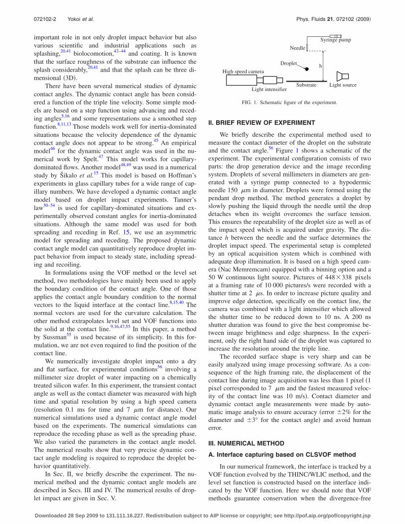
We briefly describe the experimental method used tomeasure the contact diameter of the droplet on the substrateand the contact angle.56 Figure 1 shows a schematic of theexperiment. The experimental configuration consists of twoparts: the drop generation device and the image recordingsystem. Droplets of several millimeters in diameters are gen-erated with a syringe pump connected to a hypodermicneedle 150 m in diameter. Droplets were formed using thependant drop method. The method generates a droplet byslowly pushing the liquid through the needle until the dropdetaches when its weight overcomes the surface tension.This ensures the repeatability of the droplet size as well as ofthe impact speed which is acquired under gravity. The dis-tance h between the needle and the surface determines thedroplet impact speed. The experimental setup is completedby an optical acquisition system which is combined withadequate drop illumination. It is based on a high speed cam-era Nac Memremcam equipped with a binning option and a50 W continuous light source. Pictures of 448338 pixelsat a framing rate of 10 000 pictures/s were recorded with ashutter time at 2 s. In order to increase picture quality andimprove edge detection, specifically on the contact line, thecamera was combined with a light intensifier which allowedthe shutter time to be reduced down to 10 ns. A 200 nsshutter duration was found to give the best compromise be-tween image brightness and edge sharpness. In the experi-ment, only the right hand side of the droplet was captured toincrease the resolution around the triple line.

The recorded surface shape is very sharp and can beeasily analyzed using image processing software. As a con-sequence of the high framing rate, the displacement of thecontact line during image acquisition was less than 1 pixel 1pixel corresponded to 7 m and the fastest measured veloc-ity of the contact line was 10 m/s. Contact diameter anddynamic contact angle measurements were made by auto-matic image analysis to ensure accuracy error 2% for thediameter and 3° for the contact angle and avoid humanerror.

III. NUMERICAL METHOD

A. Interface capturing based on CLSVOF method

In our numerical framework, the interface is tracked by aVOF function evolved by the THINC/WLIC method, and thelevel set function is constructed based on the interface indi-cated by the VOF function. Here we should note that VOFmethods guarantee conservation when the divergence-free

High speed camera

Substrate Light source

Needle

h

Syringe pump

Light intensifier

Droplet

FIG. 1. Schematic figure of the experiment.

072102-2 Yokoi et al. Phys. Fluids 21, 072102 2009

Downloaded 28 Sep 2009 to 131.111.16.227. Redistribution subject to AIP license or copyright; see http://pof.aip.org/pof/copyright.jsp

condition ·u=0 is precisely satisfied on staggered grids.If the velocity field does not satisfy the divergence-free con-dition, conservation is not satisfied even though a VOF typemethod is used.

1. The THINC/WLIC method

The THINC/WLIC method is a type of VOF method.The VOF function is advected by

t+ · u − · u = 0. 1

Here u is the velocity and is the characteristic function.The cell average of is the VOF function Ci,j axisymmetriccase

Ci,j =1

i,j

i,j

rdrdz . 2

The Ci,j is evolved by an approximation using a dimensionalsplitting algorithm as follows:

Ci,j = Ci,j

n −ri+1/2,jFr,i+1/2,j

n − ri−1/2,jFr,i−1/2,jn

ri,jr

+ Ci,jn ri+1/2,jur,i+1/2,j − ri−1/2,jur,i−1/2,j

ri,jrt , 3

Ci,jn+1 = Ci,j

−Fz,i,j+1/2

− Fz,i,j−1/2

z

+ Ci,jn uz,i,j+1/2 − uz,i,j−1/2

zt , 4

with

Fr,i+1/2,j = − zi,j−1/2

zi,j+1/2 ri+1/2,j

rr,i+1/2,j−ur,i+1/2,jt

is,jr,zdrdz , 5

Fz,i,j+1/2 = − zi,j+1/2

zi,j+1/2−uz,i,j+1/2t ri−1/2,j

ri+1/2,j

i,jsr,zdrdz . 6

Here Fr,i+1/2,j and Fz,i,j+1/2 are the advection fluxes for the rand z directions, respectively. The is and js are

is = i if ur,i+1/2,j 0,

i + 1 if ur,i+1/2,j 0, 7

and

js = j if uz,i,j+1/2 0,

j + 1 if uz,i,j+1/2 0. 8

The fluxes can be computed by the THINC/WLIC method orthe VOF/PLIC method. The details of the THINC/WLICmethod used in this paper are given in Refs. 33, 34, and 57.We use the THINC/WLIC method because its implementa-tion is easier than that of the VOF/PLIC method and theresults are almost the same.

2. The level set method „CLSVOF…

The level set function signed distance function isconstructed from the interface indicated by the VOF functionby a method58 which uses the fast marching method29,59 andan iterative reinitialization scheme proposed by Sussman etal.28 referred to hereafter as Sussman’s method. The levelset function within h where h is the grid spacing fromthe interface indicated by the VOF function is computed bythe fast marching method, solving the Eikonal equation

= 1. 9

Other further from the interface are calculated by Suss-man’s method, while computed by the fast marchingmethod is fixed. Sussman’s method solves the followingproblem to a steady state:

1= S1 − , 10

where 1 is artificial time and S is a smoothed sign func-tion

S =

2 + 2. 11

To reduce the iteration number of Eq. 10, we also solve thelevel set equation

t+ u · = 0, 12

before the calculation of Eq. 10. We just use a first orderupwind method for Eq. 12. This is a kind of preconditionerto make n approach n+1.

The density color function d which is used to definethe physical properties for different materials, such as den-sity and viscosity, can be generated as a smoothed Heavisidefunction

d = H , 13

with

H = 0 if − ,

1

21 +

+

1

sin

if ,

1 if , 14

where 2 represents the thickness of the transition regionbetween the liquid phase and the gas phase. In this paper,=x was used. The density function is set as d=1 for theliquid and d=0 for the gas. The density and the viscositycoefficient are calculated by

= liquid d + air1 − d , 15

= liquid d + air1 − d , 16

where liquid and air are the densities of liquid and air, andliquid and air are the viscosities of liquid and air.

072102-3 Numerical studies of the influence of the dynamic contact angle Phys. Fluids 21, 072102 2009

Downloaded 28 Sep 2009 to 131.111.16.227. Redistribution subject to AIP license or copyright; see http://pof.aip.org/pof/copyright.jsp

B. Governing equations of fluid

We use a finite volume formulation so that we use thefollowing governing equation of an integral form:

u · ndS = 0, 17

t

udV +

uu · ndS

= −1

pndS +1

2D · ndS +Fsf

+ g , 18

where u is the velocity, n the outgoing normal vector for thecontrol volume with its surface denoted by see Fig. 2, is the density, p is the pressure, D is the deformation tensorD=0.5u+ uT, Fsf is the surface tension force, and gis the acceleration due to the gravity. Our formulation is fullyconservative for cells not containing the interface, and isonly approximately conservative in cells containing the in-terface. Equations 17 and 18 are solved by a multimo-ment method based on the CIP-CSL method and VSIAM3.

We use a fractional step approach.60 Equation 18 issplit into three parts as follows:

ut+t = fNA2fNA1fAut , 19

1 advection part fA,

t

udV +

uu · ndS = 0, 20

2 nonadvection part 1 fNA1,

t

udV =1

2D · ndS +Fsf

+ g , 21

3 nonadvection part 2 fNA2,

u · ndS = 0, 22

t

udV = −1

pndS . 23

The advection part and nonadvection parts are solved by theCIP-CSL method and VSIAM3, respectively.

C. Grid

We use the grid as shown in Fig. 2. This grid is for amultimoment method CIP-CSL and VSIAM3 which usesboth values of cell averages or volume integrated averageas well as boundary averages or surface integratedaverage.61 The cell averages ui,j ,vi,j , pi,j are defined at thecell center and the boundary averages ui−1/2,j, ui,j−1/2, vi−1/2,j,and vi,j−1/2 are defined on the center of the cell boundary. Acell average and a boundary average are both used as vari-ables and these definitions are

ui,j =1

rz

ri−1/2

ri+1/2 zj−1/2

zj+1/2

ur,zdrdz , 24

ui−1/2,j =1

z

zj−1/2

zj+1/2

uri−1/2,zdz , 25

ui,j−1/2 =1

r

rj−1/2

rj+1/2

ur,zj−1/2dr . 26

D. CIP-CSL method „convection term…

The CIP-CSL method is a solver of the conservationequation

t

dV +

u · ndS = 0, 27

where is a scalar value. The CIP-CSL methods have sev-eral variations. Here the simplest one, CIP-CSL2 method,35

is explained. To avoid numerical oscillation, the CIP-CSLR0method37 should be used. First we explain the one dimen-sional case. In the one dimensional case, there are three val-ues one cell average i and two point values i−1/2 and i+1/2 between xi−1/2 and xi+1/2. Therefore we can interpolatebetween xi−1/2 and xi+1/2 by a quadratic function ix, asshown in Fig. 3,

ix = aix − xi−1/22 + bix − xi−1/2 + i−1/2, 28

with

ai =1

x2 − 6 i + 3 i−1/2 + 3 i+1/2 , 29

u ,v ,pu,v

Ω

Γ

i,j

u,v

u,v

u,v

i, j+1/2

i+1/2, j

i, j-1/2

i-1/2, j

FIG. 2. Grid used in two dimensional case. ui,j is the cell average andui−1/2,j, ui+1/2,j, vi,j−1/2, and vi,j+1/2 are the boundary averages.

FIG. 3. Schematic of the CIP-CSL method.

072102-4 Yokoi et al. Phys. Fluids 21, 072102 2009

Downloaded 28 Sep 2009 to 131.111.16.227. Redistribution subject to AIP license or copyright; see http://pof.aip.org/pof/copyright.jsp

bi =1

x6 i − 4 i−1/2 − 2 i+1/2 . 30

By using the interpolation function ix, the boundary value i−1/2 is updated by the conservation equation of a differen-tial form

t+ u

x= −

u

x. 31

A semi-Lagrangian approach is used for Eq. 31,

i−1/2 = i−1xi−1/2 − ui−1/2t if ui−1/2 0,

ixi−1/2 − ui−1/2t if ui−1/2 0, 32

t= −

u

x. 33

The cell average i is updated by a finite volume formulation

t

xi−1.2

xi+1/2

dx = −1

xFi+1/2 − Fi−1/2 , 34

where Fi−1/2 is the flux

Fi−1/2 = − xi−1/2

xi−1/2−ui−1/2t

i−1xdx if ui−1/2 0,

− xi−1/2

xi−1/2−ui−1/2t

ixdx if ui−1/2 0. 35

For multidimensional cases, a dimensional splittingmethod38 is used. In the x-direction computation, i,j

and i−1/2,j

are updated based on i,j,kn and i−1/2,j,k

n by the onedimensional CIP-CSL method. The rest of the values, such as i,j−1/2

n , are updated by time evolution converting TEC asfollows:

i,j−1/2 = i,j−1/2

n + 12 i,j

− i,jn + i,j−1

− i,j−1n . 36

In axisymmetric geometry, this formulation is little modified.Although we can use the same approach for the z-direction,for the r-directions 31 and 34 must be modified as

t+ u

r= −

r

rur

, 37

t

ri−1.2

ri+1/2

dr = −1

rixri+1/2Fi+1/2 − ri−1/2Fi−1/2 . 38

E. Viscous stress term

The viscous stress term 39 is discretized by a standardfinite volume discretization,32

t

udV =1

2D · ndS . 39

First ui,j cell average is updated. The boundary values suchas ui−1/2,j are updated by TEC as explained in the section onthe CIP-CSL method Sec III D.

F. Projection step „pressure gradient termand continuity equation…

By using the divergence of Eq. 23 and un+1 ·ndS=0, the Poisson equation

−

r

pn+1 · ndS =

1

t

ru · ndS 40

is obtained, where u is the velocity after nonadvection step1. Equation 40 is discretized

r

n+1rpn+1

i+1/2,j− r

n+1rpn+1

i−1/2,j

r

+ r

n+1zpn+1

i,j+1/2− r

n+1zpn+1

i,j−1/2

z

=1

t ri+1/2,jui+1/2,j

− ri−1/2,jui−1/2,j

r

+ri,j+1/2vi,j+1/2

− ri,j−1/2vi,j−1/2

z , 41

where

r

n+1rpn+1

i−1/2,j

2ri−1/2,j

i,jn+1 + i−1,j

n+1

pi,jn+1 − pi−1,j

n+1

r. 42

A preconditioned BiConjugate Gradient Stabilized BiCG-STAB method62 is used for the pressure Poisson equation.The convergence tolerance of the pressure Poisson equationp=10−10 is used. This means that the divergence-free con-dition is precisely satisfied. By using pn+1, the velocity ofboundary values ui−1/2,j, vi,j−1/2 are updated,

ui−1/2,jn+1 = ui−1/2,j

− 1

n+1rpn+1

i−1/2,j. 43

Other velocities ui,j, vi,j, ui,j−1/2, vi−1/2,j are updated by theTEC formula.

G. Model of surface tension force

The surface tension force appears as the surface force

Fsf = ns, 44

where is the fluid surface tension coefficient, is the localmean curvature, and ns is the unit vector normal to the inter-face. In this calculation, the surface tension force is modeledas a body force Fsf associated with the gradient of the den-sity function

Fsf = d. 45

can be computed from

= − · nls. 46

nls is evaluated from the level set function

nls =

. 47

072102-5 Numerical studies of the influence of the dynamic contact angle Phys. Fluids 21, 072102 2009

Downloaded 28 Sep 2009 to 131.111.16.227. Redistribution subject to AIP license or copyright; see http://pof.aip.org/pof/copyright.jsp

H. Contact angle implementation

1. Implementation

To impose the contact angle, we used a method devel-oped by Sussman.55 An important advantage of this methodis that we do not need to locate the position of the triple pointin the subgrid explicitly. Contact angle is taken into accountby extrapolating the liquid interface represented by the levelset function as well as the VOF function into the solid, asshown in Fig. 4.

The liquid interface is extrapolated by solving the exten-sion equation

2+ uextend · = 0, 48

where 2 is the artificial time. In this work, 2=0.5x ischosen. uextend is the extension velocity and is computed asfollows:

uextend =nwall − cot − n2

nwall − cot − n2if c 0,

nwall + cot − n2

nwall + cot − n2if c 0,

nwall if c = 0, 49

where

nwall = 0,− 1 , 50

n1 = −nls nwall

nls nwall, 51

n2 = −n1 nwall

n1 nwall, 52

c = nls · n2. 53

Here is the contact angle. The extension equation is simplysolved by using a bilinear interpolation.

2. Singularity at the triple line

In theory, there is a singularity problem at the triple line.If a no-slip condition is imposed on the solid interface thetriple line cannot move. However in reality, the triple linedoes move. In formulations using staggered grids, the singu-larity problem is avoided. The VOF function which repre-sents the liquid interface is advected by the r-component of

velocity indicated by the black circles in Fig. 5 and thez-component of velocity indicated by the black squares.

Therefore if the r-component of velocity has a finitevalue, the triple line can numerically move. In this formula-tion, the no-slip condition is imposed by extrapolating thefluid velocity into the solid as the no-slip condition is satis-fied,

ui−1/2,1 = − ui−1/2,2, 54

as shown in Fig. 5a.63 This formulation avoids the singu-larity problem because the r-component of velocity is notdefined on the solid surface. Additionally the r-component ofvelocity has been defined as the boundary average ui+1/2,j

=1 /zzi+1/2,j−1/2zi+1/2,j+1/2udz. Therefore the r-component of velocity

can have a finite value and the triple line can numericallymove along the solid surface as taking into account the no-slip condition.

In this formula, it is easy to introduce the slip length Ls

as

ui−1/2,1 =ui−1/2,2

Ls +z

2

Ls −z

2 , 55

as shown in Fig. 5b. The slip length is used to avoid thesingularity problem in formulations which define the velocityon the solid surface such as FEM. In fact a slip length existsin the real world, and has been studied by using moleculardynamics. However, we do not use the concept of slip lengthbecause our formulation does not have a singularity problem

Liquid interface

θSolid interface

unwall

n2

extendns

FIG. 4. Contact angle implementation. The dashed line represents the imagi-nary liquid interface in the solid. The contact angle is taken into account bythe imaginary liquid interface represented by the level set function.

Fluid

Solid(i,1)

(i,2)(i-1,2)

(i-1,1)

Fluid

Solid

Ls

(a) (b)

FIG. 5. Schematics no-slip boundary condition a and slip length b. Blackcircles and squares represent where r- and z-components of velocity aredefined, respectively. The arrow in the fluid represents the velocity of thefluid. The arrow in the solid represents a fictitious velocity to impose theno-slip condition. Ls is the slip length.

0

20

40

60

80

100

120

140

160

180

-0.4 -0.2 0 0.2 0.4

Con

tact

angl

e

Ucl [m/s]

Experiment

FIG. 6. Experimental measurements of contact angle. The liquid is distilledwater and the substrate is a chemically treated silicon wafer. The impactspeed is 1 m/s. The droplet diameter is 2.28 mm.

072102-6 Yokoi et al. Phys. Fluids 21, 072102 2009

Downloaded 28 Sep 2009 to 131.111.16.227. Redistribution subject to AIP license or copyright; see http://pof.aip.org/pof/copyright.jsp

and we believe that the slip length is much smaller than themesh size.

IV. DYNAMIC CONTACT ANGLE MODEL

Figure 6 shows the experimental values of contact anglemeasured during the impact of a 2.28 mm diameter droparriving at 1 m/s.56 Here we would like to explain the detailof advancing receding contact angles. Two types of advanc-ing receding contact angles are experimentally defined:“dynamic” advancing receding contact angle and “static”advancing receding contact angle. In the droplet impactexperiment, the dynamic advancing receding contact angleda dr is the angle which is measured during dropletspreading recoiling. A complex interaction between thefluid viscosity, the surface tension, the inertia, and the sub-strate results in the dynamic advancing receding contactangle being a function of the velocity of the contact line UCL.In the measurements, the dynamic advancing receding con-

tact angle tends to a limit as UCL increases decreases, asshown in Fig. 6. We name these limits the maximum dy-namic advancing angle mda and the minimum dynamicreceding angle mdr.

In contrast, the static advancing receding contact anglesa sr is defined as the maximum minimum angle ob-served when the triple line speed is zero or nearly zero i.e.,quasistatic.45

We propose a dynamic contact angle model. The modelis based on Tanner’s law50–54

Ca = kd − e3, 56

for capillary-dominated situation low Ca number, where Cais the Capillary number CaUCL / and k is a material-related constant which is empirically determined. The anglesd and e are the dynamic contact angle and the equilibriumcontact angle, respectively. Another approximation is usedfor the inertia-dominated situation. When inertia is dominanthigh Ca number, the constant angles, mda and mdr, areused

dUCL = mda if UCL 0,

mdr if UCL 0, 57

as shown in Fig. 6. The proposed model is based on Eqs.56 and 57.

The dynamic contact angle model simply consists ofEqs. 56 and 57 as

UCL = mine + Ca

ka 1/3

,mda if UCL 0,

maxe + Ca

kr 1/3

,mdr if UCL 0, 58

where ka and kr are material-related parameters for advanc-ing and receding, respectively. These parameters ka and kr

are determined as the best fit parameters to the measurement

0

20

40

60

80

100

120

140

160

180

-0.4 -0.2 0 0.2 0.4

Con

tact

angl

e[d

eg]

UCL [m/s]

Experimentka = 9 x 10-9, kr = 9 x 10-8

FIG. 7. An approximation to the experimental data Fig. 6 by Eq. 58. Asparameters for the contact angle model, mda=114°, e=90°, mdr=52°, ka

=9.010−9, and kr=9.010−8 are used. The contact angle model is referredas model I.

0[ms]

2[ms]

4[ms]

10[ms]

15[ms]

30[ms]

0[ms]

2[ms]

4[ms]

10[ms]

15[ms]

30[ms]30[ms]

15[ms]

10[ms]

4[ms]

2[ms]

0[ms]2.28[mm] 2.28[mm]0[ms]

2[ms]

4[ms]

10[ms]

15[ms]

30[ms]

FIG. 8. Color online Comparison of appearance between the experimental and numerical results for model I. The left and right hand sides are experimentaland numerical results, respectively. Although the numerical results appear 3D, the simulation is two dimensional. The grid size is 100100. The snapshotswere not obtained from the same experiment in which the dynamic contact angle and the diameter were measured, although the conditions are as similar aspossible. This is because the experiment to measure contact angle and diameter captures only the right hand side of the droplet in order to increase theresolution around the triple line enhanced online. URL: http://dx.doi.org/10.1063/1.3158468.1, URL: http://dx.doi.org/10.1063/1.3158468.2

072102-7 Numerical studies of the influence of the dynamic contact angle Phys. Fluids 21, 072102 2009

Downloaded 28 Sep 2009 to 131.111.16.227. Redistribution subject to AIP license or copyright; see http://pof.aip.org/pof/copyright.jsp

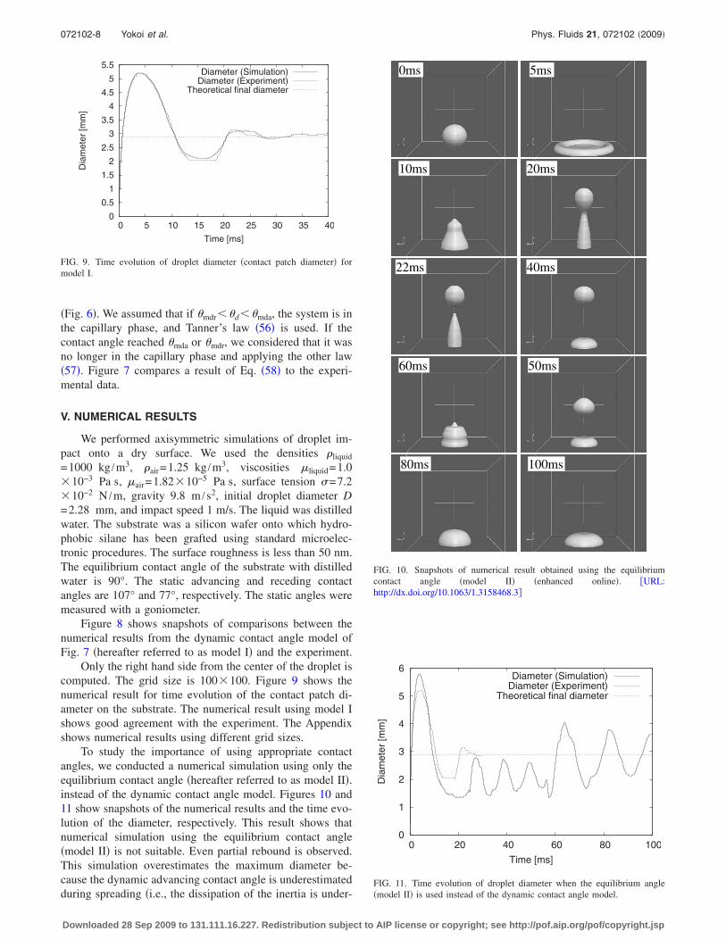
Fig. 6. We assumed that if mdrdmda, the system is inthe capillary phase, and Tanner’s law 56 is used. If thecontact angle reached mda or mdr, we considered that it wasno longer in the capillary phase and applying the other law57. Figure 7 compares a result of Eq. 58 to the experi-mental data.

V. NUMERICAL RESULTS

We performed axisymmetric simulations of droplet im-pact onto a dry surface. We used the densities liquid

=1000 kg /m3, air=1.25 kg /m3, viscosities liquid=1.010−3 Pa s, air=1.8210−5 Pa s, surface tension =7.210−2 N /m, gravity 9.8 m /s2, initial droplet diameter D=2.28 mm, and impact speed 1 m/s. The liquid was distilledwater. The substrate was a silicon wafer onto which hydro-phobic silane has been grafted using standard microelec-tronic procedures. The surface roughness is less than 50 nm.The equilibrium contact angle of the substrate with distilledwater is 90°. The static advancing and receding contactangles are 107° and 77°, respectively. The static angles weremeasured with a goniometer.

Figure 8 shows snapshots of comparisons between thenumerical results from the dynamic contact angle model ofFig. 7 hereafter referred to as model I and the experiment.

Only the right hand side from the center of the droplet iscomputed. The grid size is 100100. Figure 9 shows thenumerical result for time evolution of the contact patch di-ameter on the substrate. The numerical result using model Ishows good agreement with the experiment. The Appendixshows numerical results using different grid sizes.

To study the importance of using appropriate contactangles, we conducted a numerical simulation using only theequilibrium contact angle hereafter referred to as model II.instead of the dynamic contact angle model. Figures 10 and11 show snapshots of the numerical results and the time evo-lution of the diameter, respectively. This result shows thatnumerical simulation using the equilibrium contact anglemodel II is not suitable. Even partial rebound is observed.This simulation overestimates the maximum diameter be-cause the dynamic advancing contact angle is underestimatedduring spreading i.e., the dissipation of the inertia is under-

0

0.5

1

1.5

2

2.5

3

3.5

4

4.5

5

5.5

0 5 10 15 20 25 30 35 40

Dia

met

er[m

m]

Time [ms]

Diameter (Simulation)Diameter (Experiment)

Theoretical final diameter

FIG. 9. Time evolution of droplet diameter contact patch diameter formodel I.

0ms 5ms

10ms 20ms

22ms 40ms

50ms60ms

80ms 100ms

20ms

22ms 40ms

FIG. 10. Snapshots of numerical result obtained using the equilibriumcontact angle model II enhanced online. URL:http://dx.doi.org/10.1063/1.3158468.3

0

1

2

3

4

5

6

0 20 40 60 80 100

Dia

met

er[m

m]

Time [ms]

Diameter (Simulation)Diameter (Experiment)

Theoretical final diameter

FIG. 11. Time evolution of droplet diameter when the equilibrium anglemodel II is used instead of the dynamic contact angle model.

072102-8 Yokoi et al. Phys. Fluids 21, 072102 2009

Downloaded 28 Sep 2009 to 131.111.16.227. Redistribution subject to AIP license or copyright; see http://pof.aip.org/pof/copyright.jsp

estimated. For retreating, the receding contact angle is over-estimated. If the contact angle is overestimated during recoil,the contact angle cannot reduce the speed of the contact linesufficiently. As a result, the triple line retreats too far. Thedynamic contact angle usually reduces the speed of the tripleline. However if only 90° equilibrium angle is used, the con-tact angle does not reduce the triple line speed, and thereforethe diameter does not stabilize even after 100 ms.

We conducted a numerical simulation using the staticadvancing and receding contact angles model III, instead ofthe maximum dynamic advancing contact angle and theminimum dynamic receding contact angle, as shown in Fig.12. Figures 13 and 14 show snapshots of the numerical re-sults and time evolution of the diameter, respectively. Thenumerical results show that the behavior is different from theexperiment shown in Fig. 8. However the numerical resultsmay be better than those using the equilibrium angle modelII. During impact and spreading, the deviation is not sogreat because the substrate is hydrophobic, and thereforemda and sa are close. The maximum diameter is slightlyovershot because the static advancing contact angle is littlelower than the actual dynamic advancing contact angle.However, retreating gives a large error in terms of appear-ance as well as in the diameter prediction. This is because thereceding contact angle is considerably overestimated, as inthe simulation using the equilibrium angle model II. Thisresult shows that numerical simulation using static anglesmodel III is also not suitable.

To study the importance of using appropriate mda andmdr, we conducted a numerical simulation using 175° and 5°instead of the measured maximum dynamic advancing andminimum receding contact angles, respectively. Figure 15shows this dynamic contact angle model model IV and Fig.16 shows the numerical result. The maximum diameter isunderestimated because the dynamic advancing contactangle is overestimated, as shown in Fig. 15. This numericalresult shows that using appropriate mda and mdr is impor-tant.

To study the influences of smoothing in the dynamiccontact angle model, we conducted numerical simulations

using a sharp dynamic contact angle model model V usingka=910−9 and kr=910−9, as shown in Fig. 17. Figure 18shows the numerical result from model V. During impact andspreading, including the maximum diameter prediction, thenumerical result shows good agreement. This is because thesharp contact angle model model V for advancing UCL

0 is the same as that of model I. However the result forthe recoil phase does not agree quantitatively with experi-ment because the contact angle is underestimated in −0.2UCL0. The underestimated contact angle reduces recoil.

0

20

40

60

80

100

120

140

160

180

-0.4 -0.2 0 0.2 0.4

Con

tact

angl

e[d

eg]

UCL [m/s]

Experimentka = 9 x 10-9, kr = 9 x 10-8

FIG. 12. The dynamic contact angle model using the static advancing andreceding contact angles model III instead of dynamic advancing and re-ceding contact angles. As parameters of the contact angle model, mda

=107°, e=90°, mdr=77°, ka=9.010−9, and kr=9.010−8 are used.

0ms 4ms

10ms 15ms

20ms

30ms 100ms

25ms

FIG. 13. Snapshots of the numerical result using model III enhanced on-line. URL: http://dx.doi.org/10.1063/1.3158468.4

0

0.5

1

1.5

2

2.5

3

3.5

4

4.5

5

5.5

0 10 20 30 40 50 60 70 80

Dia

met

er[m

m]

Time [ms]

Diameter (Simulation)Diameter (Experiment)

Theoretical final diameter

FIG. 14. Time evolution of droplet diameter when model III is used.

072102-9 Numerical studies of the influence of the dynamic contact angle Phys. Fluids 21, 072102 2009

Downloaded 28 Sep 2009 to 131.111.16.227. Redistribution subject to AIP license or copyright; see http://pof.aip.org/pof/copyright.jsp

As a result, the numerical simulation did not achieve a meta-stable diameter in the time period of 13–18 ms Fig. 18.

VI. CONCLUSIONS

We conducted axisymmetric simulations for droplet im-pact onto a dry plane surface. Our numerical formulation canrobustly simulate droplet impact behavior. We introduced adynamic contact angle model based on the experimentalmeasurement. To approximate the measured values of dy-namic contact angle, we used Tanner’s law for low Ca num-ber, the maximum dynamic advancing angle and the mini-mum dynamic receding angle for high Ca number, and theequilibrium contact angle for Ca=0.

Our numerical results show that using appropriate maxi-mum and minimum angles, and smoothing of the dynamiccontact angle model are important. Numerical results ofmodel II using equilibrium angle and model III usingstatic angles showed totally different behavior from the ex-periment. Numerical results using different maximum/minimum dynamic angles model IV and smoothing modelV did not show good agreement with the experiment, either.

The contact angle model is asymmetric in terms of am-plitudes as well as smoothing, such as the experimental mea-surement. The asymmetric dynamic contact angle model isimportant in predicting precisely not only the advancingphase but also the receding phase of drop impact.

ACKNOWLEDGMENTS

Numerical computations in this work were partially car-ried out on SX8 at the Yukawa Institute for Theoretical Phys-ics, Kyoto University. The experiment was carried out whileD.V. was at Laboratoire des Ecoulements Géophysiques etIndustriels, University Joseph Fourier. D.V. acknowledges fi-nancial support from the MENRT through Project No. 2911. We acknowledge the support of the EPSRC.

APPENDIX: RESOLUTION STUDY

Figure 19 shows the numerical results obtained withthree different grid sizes 5050, 100100, and 200200, respectively with the parameters of the model heldfixed. The results are close. In particular the final diameter

0

20

40

60

80

100

120

140

160

180

-0.4 -0.2 0 0.2 0.4

Con

tact

angl

e[d

eg]

UCL [m/s]

Experimentka = 9 x 10-9, kr = 9 x 10-8

FIG. 15. The dynamic contact angle model model IV using mda=175°,mdr=5°, ka=9.010−9, and kr=9.010−8.

0

0.5

1

1.5

2

2.5

3

3.5

4

4.5

5

5.5

0 5 10 15 20 25 30 35 40

Dia

met

er[m

m]

Time [ms]

Diameter (Simulation)Diameter (Experiment)

Theoretical final diameter

FIG. 16. Time evolution of droplet diameter when model IV is used.

0

20

40

60

80

100

120

140

160

180

-0.4 -0.2 0 0.2 0.4

Con

tact

angl

e[d

eg]

UCL [m/s]

Experimentka = 9 x 10-9, kr = 9 x 10-9

FIG. 17. Sharp dynamic contact angle model model V. mda=114°, e

=90°, mdr=52°, ka=910−9, and kr=910−9 are used.

0

0.5

1

1.5

2

2.5

3

3.5

4

4.5

5

5.5

0 5 10 15 20 25 30 35 40

Dia

met

er[m

m]

Time [ms]

Diameter (Simulation)Diameter (Experiment)

Theoretical final diameter

FIG. 18. Time evolution of droplet diameter using model V.

072102-10 Yokoi et al. Phys. Fluids 21, 072102 2009

Downloaded 28 Sep 2009 to 131.111.16.227. Redistribution subject to AIP license or copyright; see http://pof.aip.org/pof/copyright.jsp

and the time of the first rebound are insensitive to the reso-lution. We are therefore confident that the 100100 gridused in this article is sufficiently accurate, while costing 1

16ththat of the 200200 grid.

1F. H. Harlow and J. P. Shannon, “The splash of a liquid drop,” J. Appl.Phys. 38, 3855 1967.

2K. Tsurutani, M. Yao, J. Senda, and H. Fujimoto, “Numerical analysis ofthe deformation process of a droplet impinging upon a wall,” JSME Int. J.,Ser. II 33, 555 1990.

3G. Trapaga and J. Szekely, “Mathematical modeling of the isothermalimpingement of liquid droplets in spraying processes,” Metall. Trans. B22, 901 1991.

4Y. D. Shikhmurzaev, “The moving contact line on a smooth solid surface,”Int. J. Multiphase Flow 19, 589 1993.

5J. Fukai, Z. Zhao, D. Poulikakos, C. M. Megaridis, and O. Miyatake,“Modeling of the deformation of a liquid droplet impinging upon a flatsurface,” Phys. Fluids A 5, 2588 1993.

6A. Karl, K. Anders, M. Rieber, and A. Frohn, “Deformation of liquiddroplets during collisions with hot walls: Experiment and numerical re-sults,” Part. Part. Syst. Charact. 13, 186 1996.

7M. Bertagnolli, M. Marchese, G. Jacucci, I. St. Doltsinis, and S. Noelting,“Thermomechanical simulation of the splashing of ceramic droplets on arigid substrate,” J. Comput. Phys. 133, 205 1997.

8M. Bussmann, S. Chandra, and J. Mostaghimi, “Modeling the splash of adroplet impacting a solid surface,” Phys. Fluids 12, 3121 2000.

9M. Renardy, Y. Renardy, and J. Li, “Numerical simulation of movingcontact line problems using a volume-of-fluid method,” J. Comput. Phys.171, 243 2001.

10R. Rioboo, M. Marengo, and C. Tropea, “Time evolution of liquid dropimpact onto solid, dry surfaces,” Exp. Fluids 33, 112 2002.

11M. Pasandideh-Fard, S. Chandra, and J. Mostaghimi, “A three-dimensional model of droplet impact and solidification,” Int. J. Heat MassTransfer 45, 2229 2002.

12Y. Renardy, S. Popinet, L. Duchemin, M. Renardy, S. Zaleski, C.Josserand, M. A. Drumwright-Clarke, D. Richard, C. Clanet, and D.Quere, “Pyramidal and toroidal water drops after impact on a solid sur-face,” J. Fluid Mech. 484, 69 2003.

13M. Francois and W. Shyy, “Computations of drop dynamics with the im-mersed boundary method. Part 2. Drop impact and heat transfer,” Numer.Heat Transfer, Part B 44, 119 2003.

14D. C. D. Roux and J. J. Cooper-White, “Dynamics of water spreading ona glass surface,” J. Colloid Interface Sci. 277, 424 2004.

15S. Sikalo, H.-D. Wilhelm, I. V. Roisman, S. Jakirli, and C. Tropea, Dy-namic contact angle of spreading droplets: Experiments and simulations,”Phys. Fluids 17, 062103 2005.

16H. Liu, S. Krishnan, S. Marella, and H. S. Udaykumar, “Sharp interfaceCartesian grid method II: A technique for simulating droplet interactions

with surfaces of arbitrary shape,” J. Comput. Phys. 210, 32 2005.17I. S. Bayer and C. M. Megaridis, “Contact angle dynamics in droplets

impacting on flat surfaces with different wetting characteristics,” J. FluidMech. 558, 415 2006.

18H. Ding and P. D. M. Spelt, “Inertial effects in droplet spreading: A com-parison between diffuse-interface and level-set simulations,” J. FluidMech. 576, 287 2007.

19S. A. Zakerzadeh, “Applying dynamic contact angles to a three-dimensional VOF model,” Ph.D. thesis, University of Toronto, 2008.

20A. L. Yarin, “Drop impact dynamics: Splashing, spreading, receding,bouncing,” Annu. Rev. Fluid Mech. 38, 159 2006.

21S. O. Unverdi and G. Tryggvason, “A front tracking method for viscous,incompressible multi-fluid flow,” J. Comput. Phys. 100, 25 1992.

22S. Popinet and S. Zaleski, “Bubble collapse near a solid boundary: Anumerical study of the influence of viscosity,” J. Fluid Mech. 464, 1372002.

23C. W. Hirt and B. D. Nichols, “Volume of fluid VOF methods for thedynamic of free boundaries,” J. Comput. Phys. 39, 201 1981.

24D. L. Youngs, “Time-dependent multi-material flow with large fluid dis-tortion,” in Numerical Methods for Fluid Dynamics, edited by K. W. Mor-ton and M. J. Baines Academic, New York, 1982, Vol. 24, pp. 273–285.

25J. Li, “Calcul d’interface affine par Morceaux piecewise linear interfacecalculation,” Acad. Sci., Paris, C. R. 320, 391 1995.

26R. Scardovelli and S. Zaleski, “Direct numerical simulation of free-surfaceand interfacial flow,” Annu. Rev. Fluid Mech. 31, 567 1999.

27S. Osher and J. A. Sethian, “Front propagating with curvature-dependentspeed: Algorithms based on Hamilton-Jacobi formulation,” J. Comput.Phys. 79, 12 1988.

28M. Sussman, P. Smereka, and S. Osher, “A level set approach for captur-ing solution to incompressible two-phase flow,” J. Comput. Phys. 114,146 1994.

29J. A. Sethian, Level Set Methods and Fast Marching Methods CambridgeUniversity Press, Cambridge, 1999.

30S. Osher and R. Fedkiw, “Level set methods and dynamic implicit sur-faces,” Applied Mathematical Sciences Springer-Verlag, New York,2003, No. 153.

31K. Yokoi and F. Xiao, “Mechanism of structure formation in circular hy-draulic jumps: Numerical studies of strongly deformed free surface shal-low flows,” Physica D 161, 202 2002.

32M. Sussman and E. G. Puckett, “A coupled level set and volume-of-fluidmethod for computing 3D and axisymmetric incompressible two-phaseflows,” J. Comput. Phys. 162, 301 2000.

33K. Yokoi, “Efficient implementation of THINC scheme: A simple andpractical smoothed VOF algorithm,” J. Comput. Phys. 226, 1985 2007.

34K. Yokoi, “A numerical method for free-surface flows and its applicationto droplet impact on a thin liquid layer,” J. Sci. Comput. 35, 372 2008.

35T. Yabe, R. Tanaka, T. Nakamura, and F. Xiao, “An exactly conservativesemi-Lagrangian scheme CIP-CSL in one dimension,” Mon. WeatherRev. 129, 332 2001.

36T. Yabe, F. Xiao, and T. Utsumi, “Constrained interpolation profile methodfor multiphase analysis,” J. Comput. Phys. 169, 556 2001.

37F. Xiao, T. Yabe, X. Peng, and H. Kobayashi, “Conservative andoscillation-less atmospheric transport schemes based on rational func-tions,” J. Geophys. Res. 107, 4609 2002.

38F. Xiao, A. Ikebata, and T. Hasegawa, “Numerical simulations of free-interface fluids by a multi integrated moment method,” Comput. Struct.83, 409 2005.

39F. Xiao, R. Akoh, and S. Ii, “Unified formulation for compressible andincompressible flows by using multi integrated moments II: Multi-dimensional version for compressible and incompressible flows,” J. Com-put. Phys. 213, 31 2006.

40J. U. Brackbill, D. B. Kothe, and C. Zemach, “A continuum method formodeling surface tension,” J. Comput. Phys. 100, 335 1992.

41P. Tsai, S. Pacheco, C. Pirat, L. Lefferts, and D. Lohse, “Drop impact uponmicro- and nanostructured superhydrophobic surfaces,” Langmuir inpress.

42D. L. Hu, B. Chan, and J. W. M. Bush, “The hydrodynamics of waterstrider locomotion,” Nature London 424, 663 2003.

43D. L. Hu and J. W. M. Bush, “Meniscus-climbing insects,” Nature Lon-don 437, 733 2005.

44J. W. M. Bush and D. L. Hu, “Walking on water: Biolocomotion at theinterface,” Annu. Rev. Fluid Mech. 38, 339 2006.

45E. B. Dussan, “On the spreading of liquids on solid surfaces: Static anddynamic contact lines,” Annu. Rev. Fluid Mech. 11, 371 1979.

0

0.5

1

1.5

2

2.5

3

3.5

4

4.5

5

5.5

0 5 10 15 20 25 30 35 40

Dia

met

er[m

m]

Time [ms]

Diameter (Experiment)Theoretical final diameter

Diameter (50x50)Diameter (100x100)Diameter (200x200)

FIG. 19. Time evolution of droplet diameter using 5050, 100100, and200200 grid resolutions. The experimental data are plotted as “+” to avoidcluttering the figure.

072102-11 Numerical studies of the influence of the dynamic contact angle Phys. Fluids 21, 072102 2009

Downloaded 28 Sep 2009 to 131.111.16.227. Redistribution subject to AIP license or copyright; see http://pof.aip.org/pof/copyright.jsp

46L. M. Hocking, “The motion of a drop on a rigid surface,” Proceedings ofthe Second International Colloquium on Drops and Bubbles, 1982, PaperNo. JPL-NASA 82-7, p. 315.

47P. D. M. Spelt, “A level-set approach for simulations of flows with mul-tiple moving contact lines with hysteresis,” J. Comput. Phys. 207, 3892005.

48R. L. Hoffman, “A study of the advancing interface. I. Interface shape inliquid.gas systems,” J. Colloid Interface Sci. 50, 228 1975.

49S. F. Kistler, “Hydrodynamics of wetting,” in Wettability, edited by J. C.Berg Dekker, New York, 1993, p. 311.

50L. Tanner, “The spreading of silicon oil drops on horizontal surfaces,” J.Phys. D 12, 1473 1979.

51P. Ehrhard and S. H. Davis, “Non-isothermal spreading of liquid drops onhorizontal plates,” J. Fluid Mech. 229, 365 1991.

52P. J. Haley and M. J. Miksis, “The effect of the contact line on dropletspreading,” J. Fluid Mech. 223, 57 1991.

53Y. D. Shikhmurzaev, “Moving contact lines in liquid/liquid/solid sys-tems,” J. Fluid Mech. 334, 211 1997.

54Y. D. Shikhmurzaev, Capillary Flows With Forming Interfaces Chapman& Hall/CRC, Boca Raton, 2007.

55M. Sussman, “An adaptive mesh algorithm for free surface flows in gen-eral geometries,” in Adaptive Method of Lines Chapman & Hall/CRC,Boca Raton, 2002.

56D. Vadillo, “Characterization of hydrodynamics phenomena during dropimpact onto different types of substrates,” Ph.D. thesis, University JosephFourier, 2006.

57F. Xiao, Y Honma and T. Kono, “A simple algebraic interface capturingscheme using hyperbolic tangent function,” Int. J. Numer. Methods Fluids48, 1023 2005.

58K. Yokoi, “Numerical method for complex moving boundary problems ina Cartesian fixed grid,” Phys. Rev. E 65, 055701R 2002.

59D. Adalsteinsson and J. A. Sethian, “The fast construction of extensionvelocities in level set methods,” J. Comput. Phys. 148, 2 1999.

60J. Kim and P. Moin, “Applications of a fractional step method to incom-pressible Navier-Stokes equations,” J. Comput. Phys. 59, 308 1985.

61F. Xiao, X. D. Peng, and X. S. Shen, “A finite-volume grid using multi-moments for geostrophic adjustment,” Mon. Weather Rev. 134, 25152006.

62H. A. van der Vorst, “Bi-CGSTAB: A fast and smoothly converging vari-ant of Bi-CG for the solution of nonsymmetric linear systems,” SIAMSoc. Ind. Appl. Math. J. Sci. Stat. Comput. 13, 631 1992.

63F. H. Harlow and E. Welch, “Numerical calculation of time-dependentviscous incompressible flow of fluids with free surface,” Phys. Fluids 8,2182 1965.

072102-12 Yokoi et al. Phys. Fluids 21, 072102 2009

Downloaded 28 Sep 2009 to 131.111.16.227. Redistribution subject to AIP license or copyright; see http://pof.aip.org/pof/copyright.jsp