arX

iv:1

805.

1073

5v2

[he

p-la

t] 1

8 A

ug 2

018

Preprint number: KYUSHU-HET-184

Numerical study of the N = 2

Landau–Ginzburg model

Okuto Morikawa1 and Hiroshi Suzuki1,∗

1Department of Physics, Kyushu University 744 Motooka, Nishi-ku, Fukuoka, 819-0395, Japan∗E-mail: hsuzuki@phys.kyushu-u.ac.jp

21/8/2018

. . . . . . . . . . . . . . . . . . . . . . . . . . . . . . . . . . . . . . . . . . . . . . . . . . . . . . . . . . . . . . . . . . . . . . . . . . . . . . .It is believed that the two-dimensional massless N = 2 Wess–Zumino model becomesthe N = 2 superconformal field theory (SCFT) in the infrared (IR) limit. We examinethis theoretical conjecture of the Landau–Ginzburg (LG) description of theN = 2 SCFTby numerical simulations on the basis of a supersymmetric-invariant momentum-cutoffregularization. We study a single supermultiplet with cubic and quartic superpotentials.From two-point correlation functions in the IR region, we measure the scaling dimensionand the central charge, which are consistent with the conjectured LG description of theA2 and A3 minimal models, respectively. Our result supports the theoretical conjectureand, at the same time, indicates a possible computational method of correlation functionsin the N = 2 SCFT from the LG description.. . . . . . . . . . . . . . . . . . . . . . . . . . . . . . . . . . . . . . . . . . . . . . . . . . . . . . . . . . . . . . . . . . . . . . . . . . . . . . . . . . . . . . . . . . . . . .

Subject Index B16, B24, B34

1 typeset using PTPTEX.cls

Contents PAGE

1 Introduction 2

2 Formulation 4

2.1 The classical action 4

2.2 Momentum cutoff regularization 5

2.3 Nicolai map 6

3 Simulation setup and classification of configurations 8

4 SUSY Ward–Takahashi relation 10

5 Scaling dimension 15

6 Central charge 19

6.1 Central charge from the supercurrent correlator 20

6.2 Central charge from the energy–momentum tensor correlator 23

6.3 Central charge from the U(1) current correlator 26

7 Conclusion 26

A Symmetries and the Noether currents 27

A.1 SUSY and the supercurrent 27

A.2 Translational invariance and the energy–momentum tensor 29

A.3 U(1) symmetry and the U(1) current 30

A.4 Massless free WZ model 31

B A fast algorithm for the Jacobian computation 32

1. Introduction

In sufficiently low energies, any quantum field theory is expected to become scale invariant,

all massive modes being decoupled. Such a scale-invariant theory would be described by a

conformal field theory (CFT). If this low-energy theory gives rise to a nontrivial CFT, the

original field theory is called the Landau–Ginzburg (LG) model or the LG description of the

CFT [1]. The LG description thus provides a Lagrangian-level realization of CFT, although

the existence of the Lagrangian of the latter is not always obvious.

As an example of the LG model, the two-dimensional (2D) N = 2 massless Wess–Zumino

(WZ) model (which can be obtained by the dimensional reduction of the four-dimensional

WZ model [2]) with a quasi-homogeneous superpotential is considered to give an LG descrip-

tion of the N = 2 superconformal field theory (SCFT) [3–14]. There are various theoretical

analyses which support this correspondence [15–24]. It is, however, still difficult to prove this

conjecture directly, because the 2D N = 2 massless WZ model is strongly coupled at low

energies and perturbation theory suffers from infrared (IR) divergences; the LG description

is truly a non-perturbative phenomenon.

A non-perturbative calculational method such as the lattice field theory may provide an

alternative approach to this issue. In Ref. [25], the scaling dimension of the scalar field in the

IR limit of the 2D N = 2 massless WZ model was measured by using a lattice formulation

from Ref. [26]. The case of a single supermultiplet with a cubic superpotential W = Φ3,

which is considered to become the A2 minimal model in the IR limit, is studied. In Ref. [25],

good agreement of the scaling dimension with that of the A2 model was observed. As is well-

recognized, the lattice formulation is in general not compatible with the supersymmetry

(SUSY) that must be a crucial element of the above LG correspondence. This is also the

2

case for the lattice formulation of Ref. [26]. However, the formulation of Ref. [26] exactly

preserves one nilpotent SUSY, utilizing the existence of the the Nicolai or Nicolai–Parisi–

Sourlas map [27–30].1 Because of this exactly preserved SUSY, and because this 2D theory

is super-renormalizable, it can be argued to all orders of perturbation theory that the full

SUSY is automatically restored in the continuum limit.2 The study of Ref. [25] thus paved

the way for the numerical investigation of the N = 2 LG model, a triumph of the lattice

field theory.3

Somewhat later, in Ref. [41], the same W = Φ3 model was analyzed by using the formu-

lation in Ref. [42]; a similar result on the scaling dimension was obtained. A salient feature

of the momentum cutoff formulation of Ref. [42] is that it preserves the full set of SUSY

as well as the translational invariance even with a finite cutoff. The formulation is (almost)

identical to the dimensional reduction of the lattice formulation [43] of the 4D WZ model

on the basis of the SLAC derivative [44, 45]. Although this formulation exactly preserves

SUSY, it sacrifices the locality because of the SLAC derivative. See Ref. [46] for an analysis

of the issue of the exact SUSY and the locality. Although the SLAC derivative generally

suffers from some pathology [47–49], for the 2D N = 2 WZ model it can be argued [42] to

all orders of perturbation theory that the locality is automatically restored in the continuum

limit. This is precisely because of the exactly preserved SUSY and because this 2D theory

is super-renormalizable. Since this formulation preserves the full SUSY, the construction

of the associated Noether current, the supercurrent, is straightforward. Then, from the IR

limit of the two-point function of the supercurrent, the central charge being fairly consis-

tent with the A2 model was observed. Thus, this study again supports the conjectured LG

correspondence.

In this paper, following on from the study of Ref. [41], we carry out the numerical study of

the N = 2 LG model on the basis of the formulation of Ref. [42]. In several aspects we extend

and improve the analysis in Ref. [41]. First, we study a higher critical model W = Φ4, which

would correspond to the A3 minimal model, as well as W = Φ3 to obtain further support for

the LG correspondence and the validity of the formulation. For the scaling dimension, in this

paper we use the two-point function in the momentum space instead of the susceptibility

of Ref. [41]. Second, the numerical accuracy and the effective number of configurations in

the Monte Carlo simulation are quite improved. Third, we also measure the central charge

by using the two-point function of the energy–momentum tensor, not only by that of the

supercurrent. In Ref. [41], it was reported that the former correlation function was too noisy

for extracting the central charge; in the present paper, we avoid this problem by rewriting

the correlation function of the energy–momentum tensor by that of the supercurrent by

using SUSY Ward–Takahashi (WT) relations. It turns out that after this transformation,

the correlation function of the energy–momentum tensor is rather useful to extract the

central charge. We also repeat the calculation of the “effective central charge” in Ref. [41]

that is an analogue of the Zamolodchikov c-function [50, 51]. All our results below show a

coherence picture being consistent with the conjectured LG correspondence.

1 This feature is common to the lattice formulation of Ref. [31].2 For this issue, see also Refs. [32, 33]. Ref. [34] is a recent review of SUSY on the lattice.3 References [35–39] are preceding studies on the 2D massive N = 2 WZ model. It appears that

the 2D massless N = 2 WZ model is numerically studied in Ref. [40].

3

In view of the LG/Calabi–Yau correspondence [17, 52–54], we hope that this kind of

numerical method will eventually provide a computation method for scattering amplitudes

in a superstring theory, whose world sheet theory is given by an N = 2 SCFT but not

necessarily by the product of solvable minimal models.

2. Formulation

2.1. The classical action

It is believed that the 2D N = 2 WZ model provides the LG description of the 2D N = 2

SCFT.4 The action of the 2D WZ model can be obtained by the dimensional reduction of

the 4D N = 1 WZ model [2] whose (Euclidean) action is given by

S =

∫d4x d4θ ΦΦ−

∫d4x d2θW (Φ)−

∫d4x d2θ W (Φ). (2.1)

Here, θ and θ are Grassmann coordinates and Φ is the chiral superfield,

Φ(x, θ) = A(y) +√2

2∑

α=1

θαψα(y) +

2∑

α=1

θαθαF (y), (2.2)

consisting of a complex scalar A, a left-handed spinor ψ, and an auxiliary field F ; the

coordinate y is given by

yM = xM + i

2∑

α=1

2∑

α=1

θασMααθα for M = 0, 1, 2, 3, (2.3)

where σ0 is the unit matrix and σ1,2,3 the Pauli matrices. The superpotential W (Φ) (W (Φ))

in Eq. (2.1) is assumed to be a polynomial of the superfield Φ (Φ).

Under the dimensional reduction, we eliminate the dependence on the coordinates x2and x3. The coordinates x0 and x1 are identified with the 2D coordinates; in what follows,

we use the complex coordinates quite often:

z ≡ x0 + ix1, z ≡ x0 − ix1. (2.4)

The corresponding derivatives are given by

∂ ≡ ∂

∂z=

1

2(∂0 − i∂1) , ∂ ≡ ∂

∂z=

1

2(∂0 + i∂1) . (2.5)

4 Here, by N = 2, we mean N = (2, 2) and not N = (2, 0).

4

With these notations,5 the Euclidean action of the 2D N = 2 WZ model is given by6

S =

∫d2x

[4∂A∗∂A− F ∗F − F ∗W ′(A)∗ − FW ′(A)

+(ψ1, ψ2

)(

2∂ W ′′(A)∗

W ′′(A) 2∂

)(ψ1

ψ2

)]. (2.8)

The basic symmetries of this system, including SUSY, are summarized in Appendix A.

2.2. Momentum cutoff regularization

We quantize the system of Eq. (2.8) by employing a momentum cutoff regularization; this

approach is studied in Ref. [42]. As emphasized in Ref. [42], this regularization exactly pre-

serves important symmetries of the system, SUSY and the translational invariance. This is

the good news. The bad news is that the regularization breaks the locality. In fact, this formu-

lation is (when the integers Lµ/a are odd implying a spacetime lattice with periodic boundary

conditions; see below) nothing but the dimensional reduction of the SUSY-invariant lattice

formulation of the 4D WZ model of Ref. [43] that is based on the SLAC derivative [44, 45].

It is well recognized that the SLAC derivative generally suffers from some pathology [47–49].

On the other hand, for the 2D N = 2 WZ model, one can argue to all orders of perturbation

theory that the locality is automatically restored when the UV cutoff is removed, thanks

to the exactly preserved SUSY [42]. However, since this argument is based on perturba-

tion theory, whose validity for the present massless WZ model is not clear due to the IR

divergences, strictly speaking, the theoretical basis of our numerical simulation is not quite

obvious. Nevertheless, our numerical results below (and those of Ref. [41]) show a coherent

picture which strongly suggests the validity of the approach. We want to leave understanding

the observed validity of our formulation as a future problem.

Now, let us suppose that the system is defined in a box of physical size L0 × L1. The

Fourier transformation of each field ϕ(x) in Eq. (2.8) is then defined by

ϕ(x) =1

L0L1

∑

p

eipxϕ(p), ϕ(p) =

∫d2x e−ipxϕ(x), (2.9)

where

pµ =2π

Lµnµ, (nµ = 0,±1,±2, . . . ). (2.10)

5 Defining a two-component Dirac fermion by ψ ≡(ψ1

ψ2

)and ψγ0 ≡ (ψ1, ψ2), the 2D Dirac matrices

are given by

γ0 =

(0 11 0

), γ1 =

(0 i−i 0

), (2.6)

that is,

γz =

(0 10 0

), γz =

(0 01 0

). (2.7)

6 The Euclidean action of the auxiliary field in the Wess–Zumino model has the “wrong sign”, i.e,the sign is opposite to the Gaussian one. In this sense, the functional integral containing the Euclideanaction of the auxiliary field is merely a formal expression. We understand that the auxiliary field isalways expressed by using the equation of motion. The functional integral then becomes perfectly welldefined under this understanding. Our computation below is based on such a well-defined functionalintegral.

5

Note that

ϕ∗(p) = ϕ(−p)∗. (2.11)

After eliminating the auxiliary field F by the equation of motion, the action in Eq. (2.8) in

terms of the Fourier modes yields

S = SB +1

L0L1

∑

p

(ψ1, ψ2

)(−p)

(2ipz W ′′(A)∗∗

W ′′(A)∗ 2ipz

)(ψ1

ψ2

)(p), (2.12)

where pz ≡ (1/2)(p0 − ip1), pz ≡ (1/2)(p0 + ip1), ∗ denotes the convolution

(ϕ1 ∗ ϕ2)(p) ≡1

L0L1

∑

q

ϕ1(q)ϕ2(p− q), (2.13)

and SB is the boson part of the action,

SB ≡ 1

L0L1

∑

p

N∗(−p)N(p), N(p) ≡ 2ipzA(p) +W ′(A)∗(p). (2.14)

It is understood that the field product in W ′′(A) and W ′′(A)∗ is defined by the convolution

of Eq. (2.13).

In order to define the functional integral, we then introduce the momentum cutoff Λ and

restrict the momentum as

|pµ| ≤ Λ ≡ π

afor µ = 0 and 1. (2.15)

All dimensionful quantities are measured in units of a. For notational simplicity, we set a = 1.

With this understanding,

pµ =2π

Lµnµ, |nµ| ≤

Lµ

2. (2.16)

We then define the partition function by

Z =

∫ ∏

|pµ|≤π

dA(p)dA∗(p)

2∏

α=1

dψα(p)

2∏

α=1

dψα(p)

e−S . (2.17)

Equation (2.12) is the action in classical theory and thus is invariant under the SUSY

transformation and the translation. Since these transformations act on field variables lin-

early (see Appendix A for their explicit form) and do not change the momentum label p,

these transformations preserve the restriction on the Fourier modes in Eq. (2.16). As the

consequence, our formulation in Eq. (2.17) manifestly preserves these symmetries [42].

2.3. Nicolai map

Our definition of the partition function in the regularized level, Eq. (2.17) of the 2D N = 2

WZ model allows the Nicolai or Nicolai–Parisi–Sourlas map [27–30], which renders the parti-

tion function Gaussian integrals [42].7 The point is that the Dirac determinant in Eq. (2.17)

7 This feature is common to the lattice formulation in Refs. [25, 26].

6

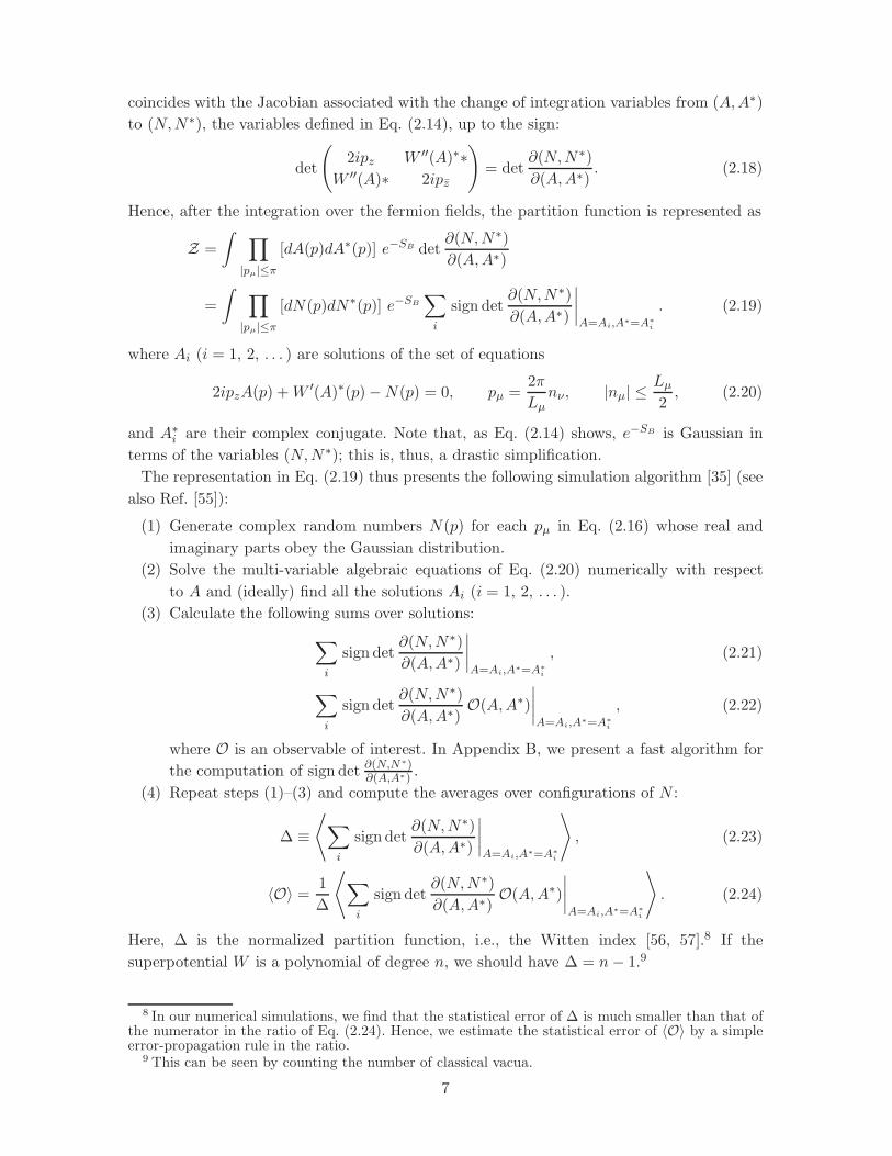
coincides with the Jacobian associated with the change of integration variables from (A,A∗)to (N,N∗), the variables defined in Eq. (2.14), up to the sign:

det

(2ipz W ′′(A)∗∗

W ′′(A)∗ 2ipz

)= det

∂(N,N∗)∂(A,A∗)

. (2.18)

Hence, after the integration over the fermion fields, the partition function is represented as

Z =

∫ ∏

|pµ|≤π

[dA(p)dA∗(p)] e−SB det∂(N,N∗)∂(A,A∗)

=

∫ ∏

|pµ|≤π

[dN(p)dN∗(p)] e−SB

∑

i

sign det∂(N,N∗)∂(A,A∗)

∣∣∣∣A=Ai,A∗=A∗

i

. (2.19)

where Ai (i = 1, 2, . . . ) are solutions of the set of equations

2ipzA(p) +W ′(A)∗(p)−N(p) = 0, pµ =2π

Lµnν, |nµ| ≤

Lµ

2, (2.20)

and A∗i are their complex conjugate. Note that, as Eq. (2.14) shows, e−SB is Gaussian in

terms of the variables (N,N∗); this is, thus, a drastic simplification.

The representation in Eq. (2.19) thus presents the following simulation algorithm [35] (see

also Ref. [55]):

(1) Generate complex random numbers N(p) for each pµ in Eq. (2.16) whose real and

imaginary parts obey the Gaussian distribution.

(2) Solve the multi-variable algebraic equations of Eq. (2.20) numerically with respect

to A and (ideally) find all the solutions Ai (i = 1, 2, . . . ).

(3) Calculate the following sums over solutions:

∑

i

sign det∂(N,N∗)∂(A,A∗)

∣∣∣∣A=Ai,A∗=A∗

i

, (2.21)

∑

i

sign det∂(N,N∗)∂(A,A∗)

O(A,A∗)

∣∣∣∣A=Ai,A∗=A∗

i

, (2.22)

where O is an observable of interest. In Appendix B, we present a fast algorithm for

the computation of sign det ∂(N,N∗)∂(A,A∗) .

(4) Repeat steps (1)–(3) and compute the averages over configurations of N :

∆ ≡⟨∑

i

sign det∂(N,N∗)∂(A,A∗)

∣∣∣∣A=Ai,A∗=A∗

i

⟩, (2.23)

〈O〉 = 1

∆

⟨∑

i

sign det∂(N,N∗)∂(A,A∗)

O(A,A∗)

∣∣∣∣A=Ai,A∗=A∗

i

⟩. (2.24)

Here, ∆ is the normalized partition function, i.e., the Witten index [56, 57].8 If the

superpotential W is a polynomial of degree n, we should have ∆ = n− 1.9

8 In our numerical simulations, we find that the statistical error of ∆ is much smaller than that ofthe numerator in the ratio of Eq. (2.24). Hence, we estimate the statistical error of 〈O〉 by a simpleerror-propagation rule in the ratio.

9 This can be seen by counting the number of classical vacua.

7

Since it is easy to generate Gaussian random numbers without any notable autocorrelation,

the above algorithm is completely free from any undesired autocorrelation and the critical

slowing down; this is a remarkable feature of this algorithm.

Unfortunately, in step (2) we cannot judge whether all the solutions of Eq. (2.20) are found

or not because we cannot know a priori the total number of solutions Ai for a given N . The

best thing we can do is to collect as many solutions as possible. For this issue, the stability

of the number of solutions under the increase of initial trial solutions in the solver algorithm,

the agreement of ∆ with the expected Witten index and the observation of expected SUSY

WT relations provide some consistency checks. In any case, the physical quantities we will

compute in what follows, the scaling dimension and the central charge, cannot be free from

the systematic error associated with the “undiscovered solutions.” It is difficult to estimate

the size of this systematic error at this time and the quoted values of the scaling dimension

and the central charge should be taken with this reservation.

3. Simulation setup and classification of configurations

In this paper we consider the 2D WZ model of Eq. (2.8) with the superpotential

W (Φ) =λ

nΦn (3.1)

with n = 3 and 4, which will be written in the abbreviated forms as W = Φ3 and W = Φ4,

respectively. We set the coupling constant

λ = 0.3 (3.2)

in units of a = 1, as in Refs. [25, 41].

To solve Eq. (2.20) with respect to A, we employ the Newton–Raphson (NR) method.10

The quality of the obtained configuration A is estimated by the following norm of the residue:

√√√√∑

p |2ipzA(p) +W ′(A)(−p)∗ −N(p)|2∑

q |N(q)|2. (3.3)

As we will see below, maximum values of this number are smaller than 10−14 for all obtained

configurations, and this is much smaller than the corresponding number in Ref. [41].

For a fixed configuration of N , we randomly generate11 initial trial configurations of A so

that we obtain 100 solutions for A allowing repetition of identical solutions; this is another

improvement compared to the setup of Ref. [41]. A randomly generated initial configuration

does not necessarily converge to a solution along the iteration in the NR method; sometimes

it diverges and does not provide any solution.12 Two solutions A1 and A2 are regarded as

10 For the generation of the configurations of N and for the computation of A and signdet ∂(N,N∗)∂(A,A∗)

we used a C++ library Eigen [58]. In particular, we extensively used the class PartialPivLU.11 The initial value of the real and imaginary parts of A(p) is generated by the Gaussian random

number with unit variance as in Ref. [41].12 In Ref. [41], the number of initial trial configurations is fixed to 100 but we found that this

choice sometimes misses some solutions for A, especially for W = Φ4.

8

identical if the norm of the difference of the solutions,√√√√∑

p |A1(p)−A2(p)|2∑q |A1(q)|2

(3.4)

is smaller than 10−13.

For both cases W = Φ3 and W = Φ4, for each box size L,

L ≡ L0 = L1, (3.5)

we generate 640 configurations of N using the Gaussian random number. The box size L is

taken as even integers from 8 to 36 for W = Φ3 and from 8 to 30 for W = Φ4.

We tabulate the classification of configurations we obtained in Tables 1–3 for W = Φ3 and

in Tables 4–6 for W = Φ4. The symbols such as (+++−)2, for example, imply the following:

For a certain configuration of N , we found four solutions Ai (i = 1, . . . , 4); sign det ∂(N,N∗)∂(A,A∗)

at three of those solutions is positive and negative at one solution. The subscript 2(= 1 +

1 + 1− 1) stands for the contribution of that N configuration to ∆ in Eq. (2.23). Table 3, for

example, shows that for L = 36 we had 13 such configurations of N out of 640 configurations.

In the tables, to indicate the quality of the configurations obtained we list ∆

from Eq. (2.23), which should reproduce 2 and 3 for W = Φ3 and W = Φ4, respectively.

For W = Φ3, our simulation gives ∆ = 2 exactly for all box sizes. For W = Φ4, ∆ deviates

from 3 for L ≥ 26 but only slightly; from this, it might be possible to roughly estimate

that the systematic error associated with the solution search (i.e., the possibility that some

solutions are missed) is less than 0.5% even for W = Φ4.

For the same purpose, we also list the one-point function,

δ ≡ 〈SB〉(L0 + 1)(L1 + 1)

− 1, (3.6)

where SB is defined in Eq. (2.14), which should identically vanish if the SUSY is exactly

preserved [36, 41].13

We also show the maximal value of the norm of the residue in Eq. (3.3) and the computation

time in core · hour on an Intel Xeon E5 2.0GHz.

Table 1: Classification of configurations for W = Φ3.

L 8 10 12 14 16

(++)2 640 640 640 639 639

(+++−)2 0 0 0 1 1

∆ 2 2 2 2 2

δ 0.0070(44) −0.0046(36) 0.0019(30) −0.0020(25) −0.0003(23)

core · hour [h] 0.77 2.23 5.5 12.37 25.62

13 For the calculation of the one-point function δ and succeeding numerical analyses, we used theprogramming language Julia [59–61].

9

Table 2: Classification of configurations for W = Φ3 (continued).

L 18 20 22 24 26

(++)2 634 636 634 637 635

(+++−)2 6 4 6 3 5

∆ 2 2 2 2 2

δ −0.0000(20) −0.0015(19) −0.0006(17) 0.0001(16) −0.0026(15)

core · hour [h] 48.97 87.03 143.83 236.62 405.28

Table 3: Classification of configurations for W = Φ3 (continued).

L 28 30 32 34 36

(++)2 634 626 633 628 627

(+++−)2 6 14 7 12 13

∆ 2 2 2 2 2

δ −0.0002(13) 0.0000(13) 0.0014(12) 0.0008(11) 0.0007(11)

core · hour [h] 649.78 963.93 1382.07 1936.52 2699.42

Table 4: Classification of configurations for W = Φ4.

L 8 10 12 14

(+++)3 638 638 638 638

(++++−)3 2 2 2 2

(+++++−−)3 0 0 0 0

(++++)4 0 0 0 0

(+++++−)4 0 0 0 0

(++)2 0 0 0 0

∆ 3 3 3 3

δ 0.0003(45) 0.0035(36) 0.0001(30) −0.0015(26)

core · hour [h] 3.73 12.8 36.1 89.55

The hot spot in our computation is the LU decomposition involved in the NRmethod whose

computational time scales as ∝ N3 for a matrix of size N . Thus, we expect that the com-

putational time scales as ∝ L6 as a function of the lattice size L. The actual computational

time shown in Fig. 1 is fairly well explained by this theoretical expectation.

4. SUSY Ward–Takahashi relation

As mentioned above, our formulation exactly preserves SUSY even with a finite cutoff. Thus,

barring the statistical error and the systematic error associated with the solution search,

SUSYWT relations should hold exactly for any parameter. The observation of these relations

10

Table 5: Classification of configurations for W = Φ4 (continued).

L 16 18 20 22

(+++)3 634 635 632 627

(++++−)3 6 5 6 13

(+++++−−)3 0 0 2 0

(++++)4 0 0 0 0

(+++++−)4 0 0 0 0

(++)2 0 0 0 0

∆ 3 3 3 3

δ 0.0006(25) 0.0014(20) 0.0024(20) 0.0023(18)

core · hour [h] 202.65 425.23 872.03 1661.22

Table 6: Classification of configurations for W = Φ4 (continued).

L 24 26 28 30

(+++)3 625 616 614 615

(++++−)3 15 23 20 22

(+++++−−)3 0 0 2 0

(++++)4 0 1 3 2

(+++++−)4 0 0 1 0

(++)2 0 0 0 1

∆ 3 3.002(2) 3.006(3) 3.002(3)

δ 0.0000(16) 0.0004(16) 0.0023(17) −0.0010(15)

core · hour [h] 2917.48 5004.37 8273.47 12905.13

thus provides a useful check of our simulation and gives a rough idea of the magnitude of

the statistical and systematic errors.

The simplest SUSY WT relation is δ = 0 for δ in Eq. (3.6), and in Tables 1–6 we have

observed that this relation is reproduced quite well in our simulation. In this section, we

present results on two further SUSY WT relations on two-point correlation functions which

follow from the identities [41]14

⟨Q1(A(p)ψ1(−p))

⟩= 0, (4.1)

〈Q2(F∗(p)ψ1(−p))〉 = 0, (4.2)

where the explicit form of the SUSY transformation is given in Appendix A.

First, Eq. (4.1) yields

2ipz 〈A(p)A∗(−p)〉 = −⟨ψ1(p)ψ1(−p)

⟩, (4.3)

14 In the present system, SUSY cannot be spontaneously broken because of the non-zero Wittenindex.

11

0

500

1000

1500

2000

2500

3000

10 15 20 25 30 35

Tim

e [

h]

L/a

L5

L6

(a) W = Φ3.

0

2000

4000

6000

8000

10000

12000

14000

10 15 20 25 30

Tim

e [

h]

L/a

L6

L7

(b) W = Φ4.

Fig. 1: Computational time as a function of the lattice size.

whose real and imaginary parts are

p1 〈A(p)A∗(−p)〉 = Re⟨ψ1(p)ψ1(−p)

⟩, (4.4)

p0 〈A(p)A∗(−p)〉 = − Im⟨ψ1(p)ψ1(−p)

⟩. (4.5)

In Figs. 2–5 we plot correlation functions in these relations as functions of −π ≤ p0 ≤ π. The

box size is the maximal one, i.e., L = 36 for W = Φ3 and L = 30 for W = Φ4. The spatial

momentum p1 is fixed to be p1 = π (the largest positive value) or p1 = 2π/L (the smallest

positive value). In the figures, the left panel corresponds to the real part relation of Eq. (4.4)

and the right one to the imaginary part of Eq. (4.5). In the plots, “bosonic” implies the

correlation function on the left-hand side of the WT relation and “fermionic” implies the

correlation function on the right-hand side. Errors are statistical only.

-450

-400

-350

-300

-250

-200

-150

-4 -3 -2 -1 0 1 2 3 4

ap0

bosonicfermionic

(a) Real part (4.4).

-250

-200

-150

-100

-50

0

50

100

150

200

250

-4 -3 -2 -1 0 1 2 3 4

ap0

bosonicfermionic

(b) Imaginary part (4.5).

Fig. 2: SUSY WT relation of Eq. (4.3) for W = Φ3, L = 36, and p1 = π.

Next, Eq. (4.2) gives the relation

〈F (p)F ∗(−p)〉 = −2ipz⟨ψ1(p)ψ1(−p)

⟩, (4.6)

12

-4000

-3500

-3000

-2500

-2000

-1500

-1000

-500

0

-4 -3 -2 -1 0 1 2 3 4

ap0

bosonicfermionic

(a) Real part (4.4).

-2500

-2000

-1500

-1000

-500

0

500

1000

1500

2000

2500

-4 -3 -2 -1 0 1 2 3 4

ap0

bosonicfermionic

(b) Imaginary part (4.5).

Fig. 3: SUSY WT relation of Eq. (4.3) for W = Φ3, L = 36, and p1 = π/18.

-320

-300

-280

-260

-240

-220

-200

-180

-160

-140

-120

-4 -3 -2 -1 0 1 2 3 4

ap0

bosonicfermionic

(a) Real part (4.4).

-200

-150

-100

-50

0

50

100

150

200

-4 -3 -2 -1 0 1 2 3 4

ap0

bosonicfermionic

(b) Imaginary part (4.5).

Fig. 4: SUSY WT relation of Eq. (4.3) for W = Φ4, L = 30, and p1 = π.

and the real and imaginary parts are given by

〈F (p)F ∗(−p)〉 = −p1Re⟨ψ1(p)ψ1(−p)

⟩+ p0 Im

⟨ψ1(p)ψ1(−p)

⟩, (4.7)

0 = −p0Re⟨ψ1(p)ψ1(−p)

⟩− p1 Im

⟨ψ1(p)ψ1(−p)

⟩. (4.8)

In Figs. 6–9 we plot correlation functions in the real part relation of Eq. (4.7); the other

conditions and conventions are the same as above. For the computation of the left-hand side

13

-2500

-2000

-1500

-1000

-500

0

-4 -3 -2 -1 0 1 2 3 4

ap0

bosonicfermionic

(a) Real part (4.4).

-1500

-1000

-500

0

500

1000

1500

-4 -3 -2 -1 0 1 2 3 4

ap0

bosonicfermionic

(b) Imaginary part (4.5).

Fig. 5: SUSY WT relation of Eq. (4.3) for W = Φ4, L = 30, and p1 = π/15.

of Eq. (4.7) we have used the representation15

〈F (p)F ∗(−p)〉 =⟨W ′(A)∗(p)W ′(A)(−p)

⟩− L0L1

=⟨|N(p)− (ip0 + p1)A(p)|2

⟩− L0L1. (4.12)

If the WT relations hold exactly, the “bosonic” points and the “fermionic” points in the

plots should coincide with each other. Overall, we observe good agreements within 1σ, as

expected. However, there still exist some deviations of order 2σ, especially in the real-part

WT relations at the largest spatial momentum p1 = π. To argue that these deviations are

a result of statistical fluctuations and not due to the omission of some solutions in our

solution search, we carried out the measurements corresponding to the left panels of Figs. 2

and 6, respectively but for L = 8, by changing the number of configurations by four times,

i.e., 640 and 2560. The results are shown in Figs. 10 and 11. We see that although for 640

configurations there exist some discrepancies between the “bosonic” and “fermionic” ones of

15 A way to derive this relation is to introduce the source term for the auxiliary field:

SJ =1

L0L1

∑

p

[F ∗(−p)J(p) + J∗(−p)F (p)] . (4.9)

Then, after a (formal) Gaussian integration over the auxiliary field, this term changes to

SJ → 1

L0L1

∑

p

[−W ′(A)(−p)J(p)− J∗(−p)W ′(A)∗(p) + J∗(−p)J(p)] . (4.10)

Therefore,

〈F ∗(−p)F (p)〉

= (L0L1)2 δ

δJ(p)

δ

δJ∗(−p)

×⟨exp

{1

L0L1

∑

q

[W ′(A)(−q)J∗(q) + J(−q)W ′(A)∗(q)− J(−q)J∗(q)]

}⟩∣∣∣∣∣J=0,J∗=0

= 〈W ′(A)∗(p)W ′(A)(−p)〉 − L0L1. (4.11)

14

-1292

-1290

-1288

-1286

-1284

-1282

-1280

-1278

-4 -3 -2 -1 0 1 2 3 4

ap0

bosonicfermionic

Fig. 6: SUSY WT relation of Eq. (4.7)

for W = Φ3, L = 36, and p1 = π.

-1300

-1200

-1100

-1000

-900

-800

-700

-600

-500

-4 -3 -2 -1 0 1 2 3 4

ap0

bosonicfermionic

Fig. 7: SUSY WT relation of Eq. (4.7)

for W = Φ3, L = 36, and p1 = π/18.

-892

-890

-888

-886

-884

-882

-880

-878

-876

-874

-872

-4 -3 -2 -1 0 1 2 3 4

ap0

bosonicfermionic

Fig. 8: SUSY WT relation of Eq. (4.7)

for W = Φ4, L = 30, and p1 = π.

-900

-850

-800

-750

-700

-650

-600

-550

-500

-450

-400

-4 -3 -2 -1 0 1 2 3 4

ap0

bosonicfermionic

Fig. 9: SUSY WT relation of Eq. (4.7)

for W = Φ4, L = 30, and p1 = π/15.

order 2σ, when we increase the number of configurations by four times, the statistical error is

halved and the discrepancies of the central values actually decrease. From this behavior, we

think that the observed discrepancies in the WT relations are due to statistical fluctuations

and they eventually disappear as the number of configurations is increased sufficiently.

Finally, we mention a general tendency of the statistical error in the correlation functions

we found through the numerical simulation. Particularly in the high momentum region, the

correlation functions of the scalar field suffer from larger statistical fluctuations than those

of the fermion field (as seen in the left panel of Fig. 2). Actually, because of this problem we

could not directly examine four-point SUSY WT relations including a four-point correlation

function of A and A∗. On the other hand, if we assume the validity of SUSYWT relations, we

can use them to rewrite some noisy correlation functions into less noisy ones. This technique

will be employed frequently in the following sections.

5. Scaling dimension

In this section, we measure the scaling dimension of the scalar field in the IR limit from

the two-point correlation function. If the expected LG correspondence for the WZ model

with W = Φn holds, the chiral superfield is identified with the chiral primary field in the

15

-22

-20

-18

-16

-14

-12

-10

-8

-4 -3 -2 -1 0 1 2 3 4

ap0

bosonicfermionic

(a) Number of configurations: 640.

-22

-20

-18

-16

-14

-12

-10

-8

-4 -3 -2 -1 0 1 2 3 4

ap0

bosonicfermionic

(b) Number of configurations: 2560.

Fig. 10: SUSY WT relation of Eq. (4.4) for W = Φ3, L = 8 and p1 = π.

-63.5

-63.4

-63.3

-63.2

-63.1

-63

-62.9

-62.8

-62.7

-4 -3 -2 -1 0 1 2 3 4

ap0

bosonicfermionic

(a) Number of configurations: 640.

-63.5

-63.4

-63.3

-63.2

-63.1

-63

-62.9

-62.8

-62.7

-4 -3 -2 -1 0 1 2 3 4

ap0

bosonicfermionic

(b) Number of configurations: 2560.

Fig. 11: SUSY WT relation of Eq. (4.7) for W = Φ3, L = 8 and p1 = π.

An−1 minimal model with the conformal dimension

h = h =1

2n. (5.1)

Thus the two-point function of the scalar field is expected to behave as

〈A(x)A∗(0)〉 ∝ 1

z2hz2h, (5.2)

for large |z|. To obtain the value of the scaling dimension h+ h, in Ref. [41], the authors

computed the susceptibility

χφ ≡ 1

a2

∫

L0L1

d2x 〈A(x)A∗(0)〉 . (5.3)

To avoid the UV ambiguity at the contact point x ∼ 0, a small region around x = 0 was

excised [25]. Then, for the scaling dimension, they obtained

1− h− h = 0.616(25)(13). (5.4)

The expected value is 1− h− h = 2/3 = 0.666 . . . for the A2 minimal model. It turns out,

however, that the susceptibility in Eq. (5.3) is quite sensitive to the size of the excised region

with the formulation of Ref. [41].

16

Here, we instead directly study the correlation function in the momentum space

〈A(p)A∗(−p)〉. The Fourier transformation of Eq. (5.2) reads (assuming h = h)

〈A(p)A∗(−p)〉 ∝ 1

(p2)1−h−h, (5.5)

for |p| small.

Also since the SUSY WT relation of Eq. (4.3) shows that

⟨ψ1(p)ψ1(−p)

⟩= −2ipz 〈A(p)A∗(−p)〉 (5.6)

instead of the two-point function of the scalar field, we may use the two-point function of

the fermion field, which is less noisy, as already mentioned.

Figure 12 shows ln〈A(p)A∗(−p)〉 as a function of ln p2 in the case of the maximal box size,

i.e., L = 36 for W = Φ3 and L = 30 for W = Φ4, respectively. We also show the fitting lines

in the UV region π√2≤ |p| < π and in the IR region 2π

L≤ |p| < 4π

L. Table 7 summarizes the

scaling dimension obtained from the linear fit in the IR region, which is one of our main

results in this paper. Recall, however, that those numbers may contain the systematic error

associated with the solutions undiscovered by the NR method.

It may be of some interest to see how the values are changed if we do not include a

few percent of “strange solutions” in Tables 1–6, such as (+++−)2 in Table 1. Thus, we

have computed the scaling dimension 1− h− h by using only the (++)2-type solutions

for W = Φ3 (L = 36) and the (+++)3-type solutions for W = Φ4 (L = 30). The result is:

1− h− h = 0.6716(82), W = Φ3, (5.7)

1− h− h = 0.7364(83), W = Φ4. (5.8)

4

5

6

7

8

9

10

11

-4 -3 -2 -1 0 1 2 3

ln<

|A(p

)|2>

ln(ap)2

UVIR

(a) W = Φ3, L = 36.

3

4

5

6

7

8

9

10

-4 -3 -2 -1 0 1 2 3

ln<

|A(p

)|2>

ln(ap)2

UVIR

(b) W = Φ4, L = 30.

Fig. 12: ln〈A(p)A∗(−p)〉 as a function of ln p2. The broken and solid lines are linear fits in

the UV and IR regions, respectively.

We also plotted in Fig. 13 the scaling dimension obtained by the above method but with

different box sizes L. Two horizontal lines show the expected values of 1− h− h from the

LG correspondence: 1− h− h = 0.666 . . . for W = Φ3 and 1− h− h = 0.75 for W = Φ4.

We clearly see the tendency that the measured scaling dimension approaches the expected

17

Table 7: Scaling dimensions obtained from the linear fit in the IR region 2πL

≤ |p| < 4πL.

W L χ2/d.o.f. 1− h− h Expected value

Φ3 36 0.506 0.682(10)(7) 0.666. . .

Φ4 30 0.358 0.747(11)(12) 0.75

value as L increases. The approach appears not quite smooth, however, so we do not try any

fitting of this plot to extract the L→ ∞ value; we suspect that this non-smoothness is due

to statistical fluctuations as we observed for the SUSY WT relation in the previous section.

From the 1− h− h case presented in Fig. 13, we estimated the systematic error associated

with the finite-volume effect. We estimate it by the maximum deviation of the central values

at the three largest volumes; the values obtained in this way are presented in the second

parentheses of 1− h− h in Table 7.

0.65

0.7

0.75

0.8

0.85

0.9

5 10 15 20 25 30 35 40

L/a

Φ3

Φ4

Fig. 13: Scaling dimensions for W = Φ3 and W = Φ4 obtained with various box sizes.

It is also interesting to see the “effective scaling dimension” that is obtained from the

fitting in some restricted intermediate region of the momentum norm |p|. This is shown

in Fig. 14. In both panels, the “effective scaling dimension” smoothly changes from that

in the IR region (which is summarized in Table 7) and approaches 1− h− h→ 1 in the

UV limit. This behavior is consistent with the expectation that the 2D N = 2 WZ models

become the free N = 2 SCFT in the UV limit, in which the chiral multiplet should have the

scaling dimension 1− h− h = 1.

18

0.6

0.65

0.7

0.75

0.8

0.85

0.9

0.95

1

0 0.5 1 1.5 2 2.5 3 3.5

1-2

h

a|p|

(a) W = Φ3, L = 36.

0.7

0.75

0.8

0.85

0.9

0.95

1

0 0.5 1 1.5 2 2.5 3 3.5

1-2

h

a|p|

(b) W = Φ4 L = 30.

Fig. 14: Scaling dimensions obtained from the linear fitting in various momentum regions

from IR to UV, 2πLn ≤ |p| < 2π

L(n+ 1), where n = 1, . . . , L− 1.

6. Central charge

In this section we consider the measurement of the central charge c, an important quantity

that characterizes CFT. This appears, in the first place, in the operator product expansion

(OPE) of the energy–momentum tensor,16

T (z)T (0) ∼ c

2z4+

2

z2T (0) +

1

z∂T (0), (6.1)

where “∼” implies “=” up to non-singular terms. The central charge of the An minimal

model is

c =3(n − 2)

n= 1, 1.5, 1.8, . . . , (6.2)

for n = 3, 4, 5, . . . .

From Eq. (6.1), assuming rotational invariance,

〈T (z)T (0)〉 = c

2z4. (6.3)

Similarly, in N = 2 SCFT, the two-point functions of the supercurrent S± and the U(1)

current J are given by

〈S+(z)S−(0)〉 = 2c

3z3, (6.4)

〈J(z)J(0)〉 = c

3z2. (6.5)

Thus, the central charge may also be obtained by computing these two-point functions.

To find the appropriate expression for the supercurrent, the energy–momentum tensor,

and the U(1) current such that they form the superconformal multiplet in N = 2 SCFT

is itself an intriguing problem, because in our system the N = 2 superconformal symmetry

is expected to emerge only in the IR limit. As explained in Appendix A, we adopt the

16 In this paper we follow the convention of Refs. [62, 63]; this convention is different from thatof Ref. [41].

19

expressions of the former two which become (gamma-) traceless for the free massless WZ

model, W ′ = 0. It appears that those expressions work as expected (see also Ref. [41]).

As in the previous section, we numerically compute the correlation function in the momen-

tum space. We consider the two-point functions of the supercurrent, the energy–momentum

tensor, and the U(1) current. As we will explain, these two-point functions are related to

each other by SUSY, which is an exact symmetry of our formulation. Using this fact, the

computation of the whole correlation function can be reduced to that for the supercurrent

correlator.

6.1. Central charge from the supercurrent correlator

The argument in Appendix A gives the supercurrent in the momentum space,

S+(p) = S+z (p) =

4π

L0L1

∑

q

i(p − q)zA(p− q)ψ2(q), (6.6)

S−(p) = S−z (p) = − 4π

L0L1

∑

q

i(p − q)zA∗(p− q)ψ2(q). (6.7)

We thus compute the two-point function 〈S+(p)S−(−p)〉. The Fourier transformation

of Eq. (6.4) is, on the other hand,

⟨S+(p)S−(−p)

⟩= L0L1

∫

L0L1

d2x e−ipx⟨S+(x)S−(0)

⟩

= L0L1

∫

L0L1

d2x e−ipx 2cz3

3(x2 + δ2)3

= L0L1−iπc6

∂3

∂p3z

( |p|δ

)2

K2(|p|δ), (6.8)

where we have introduced a regulator δ to tame the singularity at x = 0; K2 is the modified

Bessel function of the second kind. Since we are interested in the IR limit, taking the limit

|p|δ → 0, we have

⟨S+(p)S−(−p)

⟩→ L0L1

iπc

3

p2zpz. (6.9)

We fit the measured two-point function 〈S+(p)S−(−p)〉 in the IR region by this function.

We plot the two-point function 〈S+(p)S−(−p)〉 in Figs. 15 and 16 for the maximal box

size, i.e., L = 36 for W = Φ3 and L = 30 for W = Φ4. In each figure, the left panel is the

real part of the correlation function and the right one is the imaginary part. The spatial

momentum p1 is fixed to the positive minimal value, p1 = 2π/L. In these figures we also

show the function on the right-hand side of Eq. (6.9) with the central charge c obtained

from the fit in the IR region 2πL

≤ |p| < 4πL; the central charges obtained in this way are

tabulated in Table 8. Again, these numbers may contain the systematic error associated

with the solutions undiscovered by the NR method.

Compared to the result of Ref. [41] for W = Φ3,

c = 1.09(14)(31), (6.10)

the central charge we obtained is somewhat closer to the expected value with the smaller

statistical error.

20

-200

0

200

400

600

800

1000

1200

-4 -3 -2 -1 0 1 2 3 4

ap0

(a) Real part

-8000

-6000

-4000

-2000

0

2000

4000

6000

8000

-4 -3 -2 -1 0 1 2 3 4

ap0

(b) Imaginary part

Fig. 15: 〈S+(p)S−(−p)〉 for W = Φ3, L = 36, and p1 = π/18. The fitting curves

from Eq. (6.9) are also depicted.

-400

-200

0

200

400

600

800

1000

-4 -3 -2 -1 0 1 2 3 4

ap0

(a) Real part

-6000

-4000

-2000

0

2000

4000

6000

-4 -3 -2 -1 0 1 2 3 4

ap0

(b) Imaginary part

Fig. 16: 〈S+(p)S−(−p)〉 for W = Φ4, L = 30, and p1 = π/15. The fitting curves

from Eq. (6.9) are also depicted.

Table 8: The central charges obtained from the fit of the supercurrent correlator. The fitting

momentum region is 2πL

≤ |p| < 4πL.

W L χ2/d.o.f. c Expected value

Φ3 36 0.928 1.087(68)(56) 1

Φ4 30 4.606 1.413(65)(31) 1.5

In Fig. 17 we have plotted how the fitted central charge changes as a function of the

box size L. From the c presented in Fig. 17, we estimated the systematic error associated

with the finite-volume effect. We estimate it by the maximum deviation of central values

at the largest three volumes; the values obtained in this way are presented in the second

parentheses for c in Table 8.

21

0.9

1

1.1

1.2

1.3

1.4

1.5

1.6

5 10 15 20 25 30 35 40

L/a

Φ3

Φ4

Fig. 17: Central charges obtained by the fit for W = Φ3 and W = Φ4 as a function of the

box size L = 8–36.

As for Fig. 14 in the previous section, it is interesting to see how the central charge obtained

by the fit changes as a function of the fitted momentum region [41]. The result is shown

in Fig. 18. This “effective central charge” depending on the momentum region is analogous

to the supersymmetric version of the Zamolodchikov c-function [50, 51]. As expected, the

“effective central charge” changes from the IR value to c = 3 in the UV limit in which the

system is expected to become a free N = 2 SCFT.

1

1.5

2

2.5

3

3.5

0 0.5 1 1.5 2 2.5 3

c

a|p|

(a) W = Φ3 and L = 36.

1.2

1.4

1.6

1.8

2

2.2

2.4

2.6

2.8

3

0 0.5 1 1.5 2 2.5 3

c

a|p|

(b) W = Φ4 and L = 30.

Fig. 18: “Effective central charge” obtained by the fit in various momentum regions, 2πLn ≤

|p| < 2πL(n+ 1) (n = 1, . . . , L− 1).

22

6.2. Central charge from the energy–momentum tensor correlator

As discussed in Appendix A, the energy–momentum tensor T = Tzz, which is expected to

be consistent with the conformal symmetry, is given in the momentum space by

T (p) =π

L0L1

∑

q

[4(p − q)zqzA

∗(p− q)A(q)

− iqzψ2(p − q)ψ2(q) + i(p − q)zψ2(p − q)ψ2(q)]. (6.11)

It turns out that this expression as it stands leads to a very noisy two-point correlation

function. Fortunately, noting the fact that the energy–momentum tensor of Eq. (6.11) is the

SUSY transformation of the supercurrent in Eqs. (6.6) and (6.7),

T (p) =1

4Q2S

+(p)− 1

4Q2S

−(p), (6.12)

where the SUSY transformation is given in Appendix A, we can express the two-point

function of the energy–momentum tensor by a linear combination of two-point functions of

the supercurrent which are less noisy:

〈T (p)T (−p)〉 = −2ipz16

⟨S+(p)S−(−p) + S−(p)S+(−p)

⟩. (6.13)

Note that this relation holds exactly in our formulation that preserves SUSY.

The Fourier transformation of Eq. (6.3) is, by the same procedure as Eqs. (6.8) and (6.9),

〈T (p)T (−p)〉 = L0L1πc

2 · 4!∂4

∂p4z

( |p|δ

)3

K3(|p|δ)

→ L0L1πc

12

p3zpz. (6.14)

We plot the two-point function 〈T (p)T (−p)〉 of Eq. (6.13) in Figs. 19 and 20 for the

maximal box size, i.e., L = 36 for W = Φ3 and L = 30 for W = Φ4. In each figure, the left

panel is the real part of the correlation function and the right one is the imaginary part. The

spatial momentum p1 is fixed to the positive minimal value, p1 = 2π/L. In these figures we

also show the function in Eq. (6.14) with the central charge c obtained from the fit in the IR

region 2πL

≤ |p| < 4πL. The central charges obtained in this way are tabulated in Table 9; this

is another main result of this paper. Recall again, however, that these numbers may contain

the systematic error associated with the solutions undiscovered by the NR method.

Table 9: The central charges obtained from the fit of the energy–momentum tensor correlator.

The fitting momentum region is 2πL

≤ |p| < 4πL.

W L χ2/d.o.f. c Expected value

Φ3 36 1.017 1.061(36)(34) 1

Φ4 30 0.916 1.415(36)(36) 1.5

We repeated the computation of the central charge c by using only the (++)2-type solutions

for W = Φ3 (L = 36) and the (+++)3-type solutions for W = Φ4 (L = 30), to see how the

23

-500

0

500

1000

1500

2000

2500

3000

3500

-4 -3 -2 -1 0 1 2 3 4

ap0

(a) Real part

-600

-400

-200

0

200

400

600

-4 -3 -2 -1 0 1 2 3 4

ap0

(b) Imaginary part

Fig. 19: 〈T (p)T (−p)〉 for W = Φ3, L = 36, and p1 = π/18. The fitting curve of Eq. (6.14) is

also depicted.

-200

0

200

400

600

800

1000

1200

1400

1600

1800

2000

-4 -3 -2 -1 0 1 2 3 4

ap0

(a) Real part

-500

-400

-300

-200

-100

0

100

200

300

400

500

-4 -3 -2 -1 0 1 2 3 4

ap0

(b) Imaginary part

Fig. 20: 〈T (p)T (−p)〉 for W = Φ4, L = 36, and p1 = π/15. The fitting curve by Eq. (6.14) is

also depicted.

values are changed if we do not include a few percent “strange solutions.” The results are:

c = 1.057(34) (W = Φ3), (6.15)

c = 1.288(28) (W = Φ4). (6.16)

One may note that the fit in Table 9 is better than that in Table 8, in the sense that

χ2/d.o.f. is very close to 1 in the former. This is due to the fact that the real and imagi-

nary parts of the two-point correlation function of Eq. (6.13) are exactly (anti-)symmetric

under p→ −p, while the numerical data of 〈S+(p)S−(−p)〉 itself does not possess this

property.17 The number of data points is thus effectively doubled.

17 This (anti-)symmetry under p→ −p is fulfilled within the margin of the statistical error; onemay also (anti-)symmetrize the two-point function 〈S+(p)S−(−p)〉 by hand.

24

In Fig. 21, we plotted how the fitted central charge changes as a function of the box size L.

From c presented in Fig. 21, we again estimated the systematic error associated with the

finite-volume effect. The values obtained in this way are presented in the second parentheses

for c in Table 9.

Also, in Fig. 22 the “effective central charge” obtained from the fit in various momentum

regions is depicted; from IR to UV, it again shows the expected behavior analogously to the

Zamolodchikov c-function.

0.9

1

1.1

1.2

1.3

1.4

1.5

1.6

1.7

5 10 15 20 25 30 35 40

L/a

Φ3

Φ4

Fig. 21: Central charges obtained by the fit for W = Φ3 and W = Φ4 as a function of the

box size L = 8–36.

1

1.5

2

2.5

3

3.5

0 0.5 1 1.5 2 2.5 3

c

a|p|

(a) W = Φ3 and L = 36.

1.2

1.4

1.6

1.8

2

2.2

2.4

2.6

2.8

3

0 0.5 1 1.5 2 2.5 3

c

a|p|

(b) W = Φ4 and L = 30.

Fig. 22: “Effective central charge” obtained by the fit in various momentum regions, 2πLn ≤

|p| < 2πL(n+ 1) (n = 1, . . . , L− 1).

25

6.3. Central charge from the U(1) current correlator

Finally, we consider the U(1) current correlator. As discussed in Appendix A, the U(1)

current is given by

J(p) =2π

L0L1

∑

q

ψ2(p− q)ψ2(q). (6.17)

The two-point function of this current is expected to behave in the IR limit as

〈J(p)J(−p)〉 = L0L1−πc3

∂2

∂p2z

|p|δK1(|p|δ)

→ L0L1−πc3

pzpz. (6.18)

We note that the supercurrent S± can be rewritten as the SUSY transformation of J ,

S+(p) = Q2J(p), S−(p) = Q2J(p). (6.19)

Therefore,⟨S+(p)S−(−p) + S−(p)S+(−p)

⟩= −2ipz 〈J(p)J(−p)〉 . (6.20)

This shows that the computation of the U(1) current correlator is identical to the energy–

momentum tensor correlator of Eq. (6.13) up to a proportionality factor. We expect that we

would obtain almost the same results as the previous subsection, so we do not carry out the

analysis on this correlator.

7. Conclusion

In this paper, following on from the study of Ref. [41], we numerically studied the IR behav-

ior of the 2D N = 2 WZ model with the superpotentials W = Φ3 and W = Φ4. We used the

SUSY-invariant momentum-cutoff formulation which allows, because of exact symmetries, a

straightforward construction of the Noether currents, i.e., the supercurrent and the energy–

momentum tensor. The simulation algorithm is free from autocorrelation because it utilizes

the Nicolai map. From two-point correlation functions in the momentum space, we deter-

mined the scaling dimension of the scalar field (Table 7) and the central charge (Table 9) in

the IR region. It appears that these results, with the flow of the “effective central charge”

in Fig. 22, are consistent with the conjectured LG correspondence to the A2 and A3 minimal

SCFT.18

As future prospects, we may further extend the present study to WZ models with mul-

tiple superfields and more complicated superpotentials such as the ADE-type theories

in Table 10 [16] (the results of the present paper apply to the A2, A3, and E6 models).

For a possible application of the present calculational method to the superstring compact-

ification to the Calabi–Yau quintic threefold, the simulation of theW = Φ5 model will be an

important starting point. We are now considering various possible extensions of the present

study.

18 Although those numbers may contain the systematic error associated with the solutionsundiscovered by the NR method.

26

Table 10: ADE-type theories

Algebra Superpotential W Central charge c

An Φn+1, n ≧ 1 3− 6/(n + 1)

Dn Φn−1 +ΦΦ′2, n ≧ 3 3− 6/2(n − 1)

E6 Φ3 +Φ′4 3− 6/12

E7 Φ3 +ΦΦ′3 3− 6/18

E8 Φ3 +Φ′5 3− 6/30

Acknowledgments

We would like to thank Katsumasa Nakayama and Hisao Suzuki for helpful suggestions and

discussions. This work was supported by JSPS Grant-in-Aid for Scientific Research Grant

Numbers JP18J20935 (O. M.) and JP16H03982 (H. S.).

A. Symmetries and the Noether currents

In this Appendix we summarize basic symmetries of the 2D N = 2 WZ model, i.e., SUSY,

the translation, and the U(1) symmetry and the associated Noether currents, the supercur-

rent, the energy–momentum tensor, and the U(1) current. The explicit form of the former

two Noether currents is ambiguous because of freedom to add a divergence-free term and/or

a term that is proportional to the equation of motion. We remove such ambiguity by impos-

ing that they are (gamma-) traceless for the massless free WZ model. This is a natural

requirement because the massless free WZ model itself is an N = 2 SCFT which possesses

the N = 2 superconformal symmetry.

A.1. SUSY and the supercurrent

The SUSY transformation in the 2D N = 2 WZ model consists of four spinor components,

Qα (α = 1, 2) and Qα (α = 1, 2). Qα is defined by

Q1ψ1(x) = −2∂A∗(x), Q1A∗(x) = 0, (A1)

Q1F∗(x) = 2∂ψ2(x), Q1ψ2(x) = 0, (A2)

Q1A(x) = ψ1(x), Q1ψ1(x) = 0, (A3)

Q1ψ2(x) = F (x), Q1F (x) = 0, (A4)

and

Q2ψ2(x) = −2∂A∗(x), Q2A∗(x) = 0, (A5)

Q2F∗(x) = −2∂ψ1(x), Q2ψ1(x) = 0, (A6)

Q2A(x) = ψ2(x), Q2ψ2(x) = 0, (A7)

Q2ψ1(x) = −F (x), Q2F (x) = 0. (A8)

27

Qα is, on the other hand, defined by

Q1ψ1(x) = −2∂A(x), Q1A(x) = 0, (A9)

Q1F (x) = −2∂ψ2(x), Q1ψ2(x) = 0, (A10)

Q1A∗(x) = ψ1(x), Q1ψ1(x) = 0, (A11)

Q1ψ2(x) = −F ∗(x), Q1F∗(x) = 0, (A12)

and

Q2ψ2(x) = −2∂A(x), Q2A(x) = 0, (A13)

Q2F (x) = 2∂ψ1(x), Q2ψ1(x) = 0, (A14)

Q2A∗(x) = ψ2(x), Q2ψ2(x) = 0, (A15)

Q2ψ1(x) = F ∗(x), Q2F∗(x) = 0. (A16)

We see that these transformations fulfill simple anti-commutation relations,

{Q1, Q1} = −2∂, (A17)

{Q2, Q2} = −2∂, (A18)

{Q1, Q2} = {Q2, Q1} = 0, (A19)

{Qα, Qβ} = {Qα, Qβ} = 0. (A20)

The supercurrent, the Noether current associated with SUSY can be read off by considering

the localized SUSY transformation in the action. That is, under

δϕ(x) =

2∑

α=1

ξα(x)Qαϕ(x)−2∑

α=1

ξα(x)Qαϕ(x), (A21)

where ϕ stands for a generic field and ξα(x) and ξα(x) are localized Grassmann parameters,

the action changes as

δS =1

2π

∫d2x

∑

µ

[ξ1(x)∂µS

+µ (x) + ξ2(x)∂µS

−µ (x) + ξ1(x)∂µS

−µ (x) + ξ2(x)∂µS

+µ (x)

].

(A22)

Here, superscripts ± denote the U(1) charge ±1, which will be defined in Sect. A.3 below.

The definition of the supercurrent S±µ is still ambiguous because of the freedom to add a

divergence-free term and/or a term that is proportional to the equation of motion. We can

remove the ambiguity [41] by imposing the gamma-traceless condition,

∑

µ

γµ

(S±µ

S±µ

)= 0, (A23)

that is,

S±z = S±

z = 0, (A24)

for the massless free WZ model, W ′ = 0.

28

Calculating the above variation and imposing Eq. (A24), we have [41]

S+z = 4πψ2∂A, S+

z = 2πψ1W′(A), (A25)

S−z = −4πψ2∂A

∗, S−z = 2πψ1W

′(A)∗, (A26)

S+z = −2πψ2W

′(A)∗, S+z = −4πψ1∂A

∗, (A27)

S−z = −2πψ2W

′(A), S−z = 4πψ1∂A. (A28)

A.2. Translational invariance and the energy–momentum tensor

The energy–momentum tensor is the Noether current associated with the translational

invariance. To remove its ambiguity, we require the traceless condition

∑

µ

Tµµ = 0, (A29)

that is,

Tzz = Tzz = 0, (A30)

for the massless free WZ model, W ′ = 0.

The energy–momentum tensor, however, has wider ambiguity than the supercurrent and,

because of this, it is difficult to find the energy–momentum tensor which fulfills the above

requirement if we simply follow the above procedure, i.e., starting from the variation of the

action under the localized translation and then imposing the traceless condition.

A better strategy is the following: We consider the infinitesimal transformation of the form

δA(x) = −∑

µ

vµ∂µA(x), (A31)

δψ1(x) = −∑

µ

vµ∂µψ1(x)−1

2(∂vz)ψ1(x), (A32)

δψ1(x) = −∑

µ

vµ∂µψ1(x)−1

2(∂vz)ψ1(x), (A33)

δψ2(x) = −∑

µ

vµ∂µψ2(x)−1

2(∂vz)ψ2(x), (A34)

δψ2(x) = −∑

µ

vµ∂µψ2(x)−1

2(∂vz)ψ2(x), (A35)

δF (x) = −∑

µ

vµ∂µF (x). (A36)

When the parameter vµ is constant, this is simply the translation that is a symmetry of the

WZ model. When vµ ∝ ǫµνxν , this is the infinitesimal Lorentz transformation that is also a

symmetry of the WZ model. Thus, localizing the parameter vµ as vµ(x), the variation of the

action gives rise to a conserved current. By construction, this current is a combination of the

canonical energy–momentum tensor, the Lorentz current, and the equation of motion. More-

over, when the parameters vz and vz are holomorphic and anti-holomorphic, respectively,

vz = vz(z) and vz = vz(z), then Eqs. (A31)–(A36) coincide with the conformal transforma-

tion, that is an exact invariance of the massless free WZ model. As a consequence, when

29

W ′ = 0 the conserved Noether current obtained by localizing vµ as vµ(x) must generate the

conformal symmetry, i.e., it must be related to the traceless energy–momentum tensor.

In this way, from the variation of the action under Eqs. (A31)–(A36),

δS = − 1

2π

∫d2x

∑

µν

vν(x)∂µTµν(x), (A37)

we have

Tµν = −2π∂µA∗∂νA− 2π∂νA

∗∂µA

+ πδµν[2∂ρA

∗∂ρA− 2F ∗F − 2F ∗W ′(A)∗ − 2FW ′(A)

+W ′′(A)∗ψ1ψ2 +W ′′(A)ψ2ψ1

]

− π(δ0µ − iδ1µ)(δ0ν − iδ1ν)(ψ1∂ψ1 − ∂ψ1ψ1

)

− π(δ0µ + iδ1µ)(δ0ν + iδ1ν)(ψ2∂ψ2 − ∂ψ2ψ2

). (A38)

This can be written as

T (≡ Tzz) = −4π∂A∗∂A− πψ2∂ψ2 + π∂ψ2ψ2, (A39)

T (≡ Tzz) = −4π∂A∗∂A∗ − πψ1∂ψ1 + π∂ψ1ψ1, (A40)

Tzz = Tzz = −πF ∗F − πF ∗W ′(A)∗ − πFW ′(A) +π

2W ′′(A)∗ψ1ψ2 +

π

2W ′′(A)ψ2ψ1. (A41)

When W ′ = 0, the traceless condition of Eq. (A30) is clearly satisfied (note that F = −W ′∗

under the equation of motion).

A.3. U(1) symmetry and the U(1) current

We take the following U(1) transformation (γ ∈ R),

δ

(ψ1

ψ2

)(x) = iγ

(ψ1

ψ2

)(x), δ

(ψ1

ψ2

)(x) = −iγ

(ψ1

ψ2

)(x), (A42)

under which the WZ model is invariant; we have assigned the U(1) charge +1 to ψ1 and ψ2,

and −1 to ψ1 and ψ2. It turns out that, in the massless free WZ model, the U(1) current

associated with this symmetry forms the superconformal multiplet with the supercurrent

and the energy–momentum tensor.19 Localizing the parameter γ as γ(x), the associated

19 The U(1)R symmetry in the case of the superpotential W = λΦn/n would be

A(x) → exp (iγ/n)A(x), (A43)

ψα(x) → exp[−iγ(n− 2)/2n]ψα(x), (A44)

ψα(x) → exp[iγ(n− 2)/2n]ψα(x), (A45)

F (x) → exp[−iγ(n− 1)/n]F (x). (A46)

The associated Noether current, however, can be neither holomorphic nor anti-holomorphic even inthe free-field limit λ→ 0; thus it cannot be a member of the superconformal multiplet.

30

Noether current can be obtained as

δS =1

2π

∫d2x 2iγ(x)

[∂Jz(x) + ∂Jz(x)

]. (A47)

The explicit form is given by

J ≡ Jz = 2πψ2ψ2, (A48)

J ≡ Jz = 2πψ1ψ1. (A49)

It can be confirmed that the supercurrent, the energy–momentum tensor, and the U(1)

current in the above form are related by the SUSY transformation in a very simple way.

This fact provides more support for the above explicit forms of currents.

A.4. Massless free WZ model

We summarize explicit expressions for the above Noether currents in the massless free WZ

model, a free N = 2 SCFT, and confirm that they actually fulfill the N = 2 super-Virasoro

algebra as expected.

The supercurrent, the energy–momentum tensor, and the U(1) current in the holomorphic

sector are

S+(z) = 4πψ2(z)∂A(z), (A50)

S−(z) = −4πψ2(z)∂A∗(z), (A51)

T (z) = −4π∂A∗(z)∂A(z) − πψ2(z)∂ψ2(z) + π∂ψ2(z)ψ2(z), (A52)

J(z) = 2πψ2(z)ψ2(z), (A53)

and in the anti-holomorphic sector,

S+(z) = −4πψ1(z)∂A∗(z), (A54)

S−(z) = 4πψ1(z)∂A(z), (A55)

T (z) = −4π∂A∗(z)∂A(z)− πψ1(z)∂ψ1(z) + π∂ψ1(z)ψ1(z), (A56)

J(z) = 2πψ1(z)ψ1(z). (A57)

The OPEs between the component fields are given by

A(z, z)A∗(0, 0) ∼ − 1

4πln |z|2, (A58)

ψ1(z)ψ1(0) ∼1

2π

1

z, (A59)

ψ2(z)ψ2(0) ∼1

2π

1

z, (A60)

(otherwise) ∼ 0, (A61)

31

where “∼” implies “=” up to non-singular terms. Using these, we find that the above Noether

currents in the holomorphic part satisfy the OPEs of the N = 2 super-Virasoro algebra,

T (z)T (0) ∼ c

2z4+

2

z2T (0) +

1

z∂T (0), (A62)

T (z)S±(0) ∼ 3

2z2S±(0) +

1

z∂S±(0), (A63)

T (z)J(0) ∼ 1

z2J(0) +

1

z∂J(0), (A64)

S±(z)S±(0) ∼ 0, (A65)

S+(z)S−(0) ∼ 2c

3z3+

2

z2J(0) +

2

zT (0) +

1

z∂J(0), (A66)

J(z)S±(0) ∼ ±1

zS±(0), (A67)

J(z)J(0) ∼ c

3z2, (A68)

where the central charge is c = 3 corresponding to a free N = 2 SCFT.

B. A fast algorithm for the Jacobian computation

We can accelerate the computation of sign det ∂(N,N∗)∂(A,A∗) by effectively halving the size of the

matrix,

∂(N,N∗)∂(A,A∗)

=

(2ipz W ′′(A)∗∗

W ′′(A)∗ 2ipz

), (B1)

whose p, q element is

[∂(N,N∗)∂(A,A∗)

]

p,q

=

(2ipzδp,q

1L0L1

W ′′(A)(q − p)∗1

L0L1

W ′′(A)(p − q) 2ipzδp,q

)

=

(2ipzδp,q

1L0L1

W ′′(A)(p − q)†1

L0L1

W ′′(A)(p − q) 2ipzδp,q

). (B2)

Note that Eq. (B2) is a [2(L0 + 1)(L1 + 1)]× [2(L0 + 1)(L1 + 1)] matrix when the momen-

tum takes the values

pµ =2π

Lµnµ, nµ = 0,±1, . . . ,±Lµ

2, (B3)

where we have assumed that both integers L0 and L1 are even,

We write the matrix in Eq. (B2) as

∂(N,N∗)∂(A,A∗)

≡(iP W †

W iP †

). (B4)

It should be noted that the diagonal matrix P , whose p, q element is 2pzδp,q, does not have

an inverse because it has zero at p = 0; what we want to do is to remove this zero.

32

Considering the case that P and W are 3× 3 matrices for simplicity, we can confirm that

the determinant of the matrix in Eq. (B4) can be deformed as

det

λ10 W †

λ2W11 W12 W13 λ3W21 W22 W23 0

W31 W32 W33 λ4

= −|W22|2 det

λ1 W ∗11 W ∗

31

λ2 W ∗13 W ∗

33

W11 W13 λ3

W31 W33 λ4

, (B5)

where

Wij ≡1

W22det

(Wij Wi2

W2j W22

). (B6)

In an analogous way, we can write, for the general case,

det

(iP W †

W iP †

)= −|W0,0|2 det′

(iP W †

W iP †

), (B7)

where W0,0 is the component at (p, q) = (0, 0), det′ is the determinant in the subspace in

which the components with p = 0 or q = 0 are omitted, and

Wp,q =1

W0,0det

(Wp,q Wp,0

W0,q W0,0

). (B8)

Note that this is simply the determinant of a 2× 2 matrix.

Since the right-hand side of Eq. (B7) refers to the subspace in which P has an inverse, the

Jacobian can be expressed as

det

(iP W †

W iP †

)= −|W0,0|2 det′

(iP 0

W I

)det′

(I (−i)P−1W †

0 iP † − W (−i)P−1W †

)(B9)

= −|W0,0|2 det′(−PP † − PWP−1W †

). (B10)

Here, the inverse of P is given by

(P−1

)p,q

=1

2pzδp,q =

pz2|pz|2

δp,q. (B11)

Thus, substituting the matrix elements in Eq. (B2), we have

det

(iP W †

W iP †

)= − det′(−1)

∣∣∣∣1

L0L1W ′′(A)(0)

∣∣∣∣2

× det′

4|pz|2δp,q +

(1

L0L1

)2∑

l 6=0

pzlzW ′′(A)(p − l)W ′′(A)(l − q)†

,

(B12)

where for p 6= 0,

W ′′(A)(p − l) ≡ 1

W ′′(A)(0)det

(W ′′(A)(p − l) W ′′(A)(p − 0)

W ′′(A)(0 − l) W ′′(A)(0 − 0)

)

=1

W ′′(A)(0)

[W ′′(A)(p − l)W ′′(A)(0) −W ′′(A)(pW ′′(A)(−l)

]. (B13)

33

Here, the factor det′(−1) is

det′(−1) = (−1)(L0+1)(L1+1)−1 = +1, (B14)

for L0 and L1 are even.

Thus, finally, the sign of the Jacobian is given by the sign of the determinant of a matrix

with smaller dimensions [(L0 + 1)(L1 + 1)− 1]× [(L0 + 1)(L1 + 1)− 1], as

sign det

(iP W †

W iP †

)

= − det′(−1) sign det′

4|pz|2δp,q +

(1

L0L1

)2∑

l 6=0

pzlzW ′′(A)(p − l)W ′′(A)(q − l)∗

. (B15)

Since the computational cost required for the matrix determinant is O(N3) for a matrix of

size N , this representation reduces the cost by ∼ 1/8.

It turns out that the above sign is mainly negative for most of configurations of A(p).

Since the overall sign of sign det ∂(N,N∗)∂(A,A∗) is irrelevant in the expectation value of Eq. (2.24),

we regard Eq. (B15) as20

− sign det∂(N,N∗)∂(A,A∗)

. (B16)

References

[1] A. B. Zamolodchikov, Sov. J. Nucl. Phys. 44 (1986) 529 [Yad. Fiz. 44 (1986) 821].[2] J. Wess and B. Zumino, Nucl. Phys. B 70 (1974) 39. doi:10.1016/0550-3213(74)90355-1[3] P. Di Vecchia, J. L. Petersen and H. B. Zheng, Phys. Lett. 162B (1985) 327. doi:10.1016/0370-

2693(85)90932-3[4] P. Di Vecchia, J. L. Petersen and M. Yu, Phys. Lett. B 172 (1986) 211. doi:10.1016/0370-2693(86)90837-

3[5] P. Di Vecchia, J. L. Petersen, M. Yu and H. B. Zheng, Phys. Lett. B 174 (1986) 280. doi:10.1016/0370-

2693(86)91099-3[6] W. Boucher, D. Friedan and A. Kent, Phys. Lett. B 172 (1986) 316. doi:10.1016/0370-2693(86)90260-1[7] D. Gepner, Nucl. Phys. B 287 (1987) 111. doi:10.1016/0550-3213(87)90098-8[8] A. Cappelli, C. Itzykson and J. B. Zuber, Nucl. Phys. B 280 (1987) 445. doi:10.1016/0550-

3213(87)90155-6[9] A. Cappelli, Phys. Lett. B 185 (1987) 82. doi:10.1016/0370-2693(87)91532-2

[10] D. Gepner and Z. a. Qiu, Nucl. Phys. B 285 (1987) 423. doi:10.1016/0550-3213(87)90348-8[11] D. Gepner, Nucl. Phys. B 296 (1988) 757. doi:10.1016/0550-3213(88)90397-5[12] A. Cappelli, C. Itzykson and J. B. Zuber, Commun. Math. Phys. 113 (1987) 1. doi:10.1007/BF01221394[13] A. Kato, Mod. Phys. Lett. A 2 (1987) 585. doi:10.1142/S0217732387000732[14] D. Gepner, Phys. Lett. B 199 (1987) 380. doi:10.1016/0370-2693(87)90938-5[15] D. A. Kastor, E. J. Martinec and S. H. Shenker, Nucl. Phys. B 316 (1989) 590. doi:10.1016/0550-

3213(89)90060-6[16] C. Vafa and N. P. Warner, Phys. Lett. B 218 (1989) 51. doi:10.1016/0370-2693(89)90473-5[17] E. J. Martinec, Phys. Lett. B 217 (1989) 431. doi:10.1016/0370-2693(89)90074-9[18] W. Lerche, C. Vafa and N. P. Warner, Nucl. Phys. B 324 (1989) 427. doi:10.1016/0550-3213(89)90474-4[19] P. S. Howe and P. C. West, Phys. Lett. B 223 (1989) 377. doi:10.1016/0370-2693(89)91619-5[20] S. Cecotti, L. Girardello and A. Pasquinucci, Nucl. Phys. B 328 (1989) 701. doi:10.1016/0550-

3213(89)90226-5[21] P. S. Howe and P. C. West, Phys. Lett. B 227 (1989) 397. doi:10.1016/0370-2693(89)90950-7[22] S. Cecotti, L. Girardello and A. Pasquinucci, Int. J. Mod. Phys. A 6 (1991) 2427.

doi:10.1142/S0217751X91001192

20 Or we may simply say that the partition function (2.19) is defined with another negative sign.

34

[23] S. Cecotti, Int. J. Mod. Phys. A 6 (1991) 1749. doi:10.1142/S0217751X91000939[24] E. Witten, Int. J. Mod. Phys. A 9 (1994) 4783 doi:10.1142/S0217751X9400193X [hep-th/9304026].[25] H. Kawai and Y. Kikukawa, Phys. Rev. D 83 (2011) 074502 doi:10.1103/PhysRevD.83.074502

[arXiv:1005.4671 [hep-lat]].[26] Y. Kikukawa and Y. Nakayama, Phys. Rev. D 66 (2002) 094508 doi:10.1103/PhysRevD.66.094508

[hep-lat/0207013].[27] H. Nicolai, Phys. Lett. 89B (1980) 341. doi:10.1016/0370-2693(80)90138-0[28] H. Nicolai, Nucl. Phys. B 176 (1980) 419. doi:10.1016/0550-3213(80)90460-5[29] G. Parisi and N. Sourlas, Nucl. Phys. B 206 (1982) 321. doi:10.1016/0550-3213(82)90538-7[30] S. Cecotti and L. Girardello, Annals Phys. 145 (1983) 81. doi:10.1016/0003-4916(83)90172-0[31] N. Sakai and M. Sakamoto, Nucl. Phys. B 229, 173 (1983). doi:10.1016/0550-3213(83)90359-0[32] J. Giedt and E. Poppitz, JHEP 0409, 029 (2004) doi:10.1088/1126-6708/2004/09/029 [hep-th/0407135].[33] D. Kadoh and H. Suzuki, Phys. Lett. B 696, 163 (2011) doi:10.1016/j.physletb.2010.12.012

[arXiv:1011.0788 [hep-lat]].[34] D. Kadoh, PoS LATTICE 2015 (2016) 017 [arXiv:1607.01170 [hep-lat]].[35] M. Beccaria, G. Curci and E. D’Ambrosio, Phys. Rev. D 58, 065009 (1998)

doi:10.1103/PhysRevD.58.065009 [hep-lat/9804010].[36] S. Catterall and S. Karamov, Phys. Rev. D 65, 094501 (2002) doi:10.1103/PhysRevD.65.094501

[hep-lat/0108024].[37] J. Giedt, Nucl. Phys. B 726, 210 (2005) doi:10.1016/j.nuclphysb.2005.08.004 [hep-lat/0507016].[38] G. Bergner, T. Kaestner, S. Uhlmann and A. Wipf, Annals Phys. 323, 946 (2008)

doi:10.1016/j.aop.2007.06.010 [arXiv:0705.2212 [hep-lat]].[39] T. Kastner, G. Bergner, S. Uhlmann, A. Wipf and C. Wozar, Phys. Rev. D 78, 095001 (2008)

doi:10.1103/PhysRevD.78.095001 [arXiv:0807.1905 [hep-lat]].[40] S. Nicolis, arXiv:1712.07045 [hep-th].[41] S. Kamata and H. Suzuki, Nucl. Phys. B 854 (2012) 552 doi:10.1016/j.nuclphysb.2011.09.007

[arXiv:1107.1367 [hep-lat]].[42] D. Kadoh and H. Suzuki, Phys. Lett. B 684 (2010) 167 doi:10.1016/j.physletb.2010.01.022

[arXiv:0909.3686 [hep-th]].[43] J. Bartels and J. B. Bronzan, Phys. Rev. D 28 (1983) 818. doi:10.1103/PhysRevD.28.818[44] S. D. Drell, M. Weinstein and S. Yankielowicz, Phys. Rev. D 14 (1976) 487.

doi:10.1103/PhysRevD.14.487[45] S. D. Drell, M. Weinstein and S. Yankielowicz, Phys. Rev. D 14 (1976) 1627.

doi:10.1103/PhysRevD.14.1627[46] G. Bergner, JHEP 1001, 024 (2010) doi:10.1007/JHEP01(2010)024 [arXiv:0909.4791 [hep-lat]].[47] P. H. Dondi and H. Nicolai, Nuovo Cim. A 41 (1977) 1. doi:10.1007/BF02730448[48] L. H. Karsten and J. Smit, Phys. Lett. 85B (1979) 100. doi:10.1016/0370-2693(79)90786-X[49] M. Kato, M. Sakamoto and H. So, JHEP 0805 (2008) 057 doi:10.1088/1126-6708/2008/05/057

[arXiv:0803.3121 [hep-lat]].[50] A. B. Zamolodchikov, JETP Lett. 43 (1986) 730 [Pisma Zh. Eksp. Teor. Fiz. 43 (1986) 565].[51] A. Cappelli and J. I. Latorre, Nucl. Phys. B 340 (1990) 659. doi:10.1016/0550-3213(90)90463-N[52] S. Cecotti, Nucl. Phys. B 355 (1991) 755. doi:10.1016/0550-3213(91)90493-H[53] B. R. Greene, C. Vafa and N. P. Warner, Nucl. Phys. B 324 (1989) 371. doi:10.1016/0550-

3213(89)90471-9[54] E. Witten, Nucl. Phys. B 403 (1993) 159 [AMS/IP Stud. Adv. Math. 1 (1996) 143] doi:10.1016/0550-

3213(93)90033-L [hep-th/9301042].[55] M. Luscher, Commun. Math. Phys. 293, 899 (2010) doi:10.1007/s00220-009-0953-7 [arXiv:0907.5491

[hep-lat]].[56] E. Witten, Nucl. Phys. B 202 (1982) 253. doi:10.1016/0550-3213(82)90071-2[57] S. Cecotti and L. Girardello, Phys. Lett. 110B (1982) 39. doi:10.1016/0370-2693(82)90947-9[58] http://eigen.tuxfamily.org/

[59] http://julialang.org/

[60] J. Bezanson, S. Karpinski, V. B. Shah and A. Edelman, arXiv:1209.5145 [cs.PL].[61] J. Bezanson, A. Edelman, S. Karpinski and V. B. Shah, arXiv:1411.1607 [cs.MS].[62] J. Polchinski, “String theory. Vol. 1: An introduction to the bosonic string,” Cambridge University

Press, 1998, 402 p.[63] J. Polchinski, “String theory. Vol. 2: Superstring theory and beyond,” Cambridge University Press,

1998, 531 p.

35