numerical study on aerofoil stall - :: welcome to ijerest :: · · 2015-05-11this aerofoil has...
TRANSCRIPT
International Journal of Emerging Researches in Engineering Science and Technology-
Vol-2-Issue-4-April-2015-ISSN: 2393-9184
27
Abstract—This work involves usage of Reynolds Averaged
Navier Stokes Equation (RANSE) based Computational Fluid
Dynamics (CFD) approach for the determination of stall angle
for Wortmann FX 79-W-151 aerofoil. Geometrical modelling of
this aerofoil has been done using ANSYS ICEM CFD and
simulations have been carried out using ANSYS CFX. Pitch
motion which is a rotation about y-axis and occurring in x-z
plane has been depicted here as yaw motion i.e. rotation about z
axis in x-y plane so that the flow around the aerofoil section can
be studied during rotation.Simulation of flow has been
accomplished for various angles of attack for determining both
static and dynamic stall. The limitation of RANSE solver with the
angle of attack and the subsequent flow separation has also been
studied.
Index Terms—Aerodynamics,CFD,Dynamic stall,Static stall.
I. INTRODUCTION
OMPUTATIONAL FLUID DYNAMICS (CFD) involves
solving of fluid flow problems by numerically solving the
Navier-Stokes equations. Navier-stokes equations are of
prime importance as they help solve majority of fluid flow
problems as its simplification leads us to Euler’s equation, Potential equations and Linearized potential equations. CFD
helps in easier identification of flaws in the design and
accurately predicts the fluid and thermal flows, thereby saving
considerable time and cost in the production process. Thus
CFD finds its application in various fields such as aerospace,
marine, medical, automotive and chemical industries.
In the present work, aerodynamic study of a flow around an
aerofoil has been studied. Stall is an unfavorable condition
that exists when the lift on the aerofoil decreases on increase
in the angle of attack. This situation is highly undesirable as
the aircraft will start spinning downwards losing its altitude.
On reviewing various literatures, it can be understood that a
quite a number of wind tunnel experiments have been done in
estimating static and dynamic stall. Numerical studies using
panel methods and Reynolds Averaged Navier Stokes
Equation (RANSE) based CFD have been limited only to the
Manuscript submitted for review on 20 January 2015.This work was
supported by the Department of Mechanical engineering, SSET, Ernakulam,
India.
Praphul T, B.Tech, Mechanical engineering, SSET, Ernakulam, India. (e-
mail: [email protected]).
Dr. Sheeja Janardhanan,Associate Professor, Department of Mechanical
Engineering, SSET, Ernakulam, India. (e-
mail:[email protected]).
estimation of static stall. Thus the idea of this work is mooted
based on [2]. This work deals with the measurements with
sinusoidal pitching and constant angular velocities and
dynamic stall characteristics. Under dynamic stall conditions,
maximum value of lift coefficient was up to 80% higher than
that for static lift. In the present work, pitch (rotation about y-
axis) motions in x-z plane have been transformed to the x-y
plane and consequent yaw (rotation about z-axis) motions
have been targeted to find out stall angles in static and
dynamic motions of the aerofoil.
II. PROBLEM FORMULATION
A. Geometrical modelling
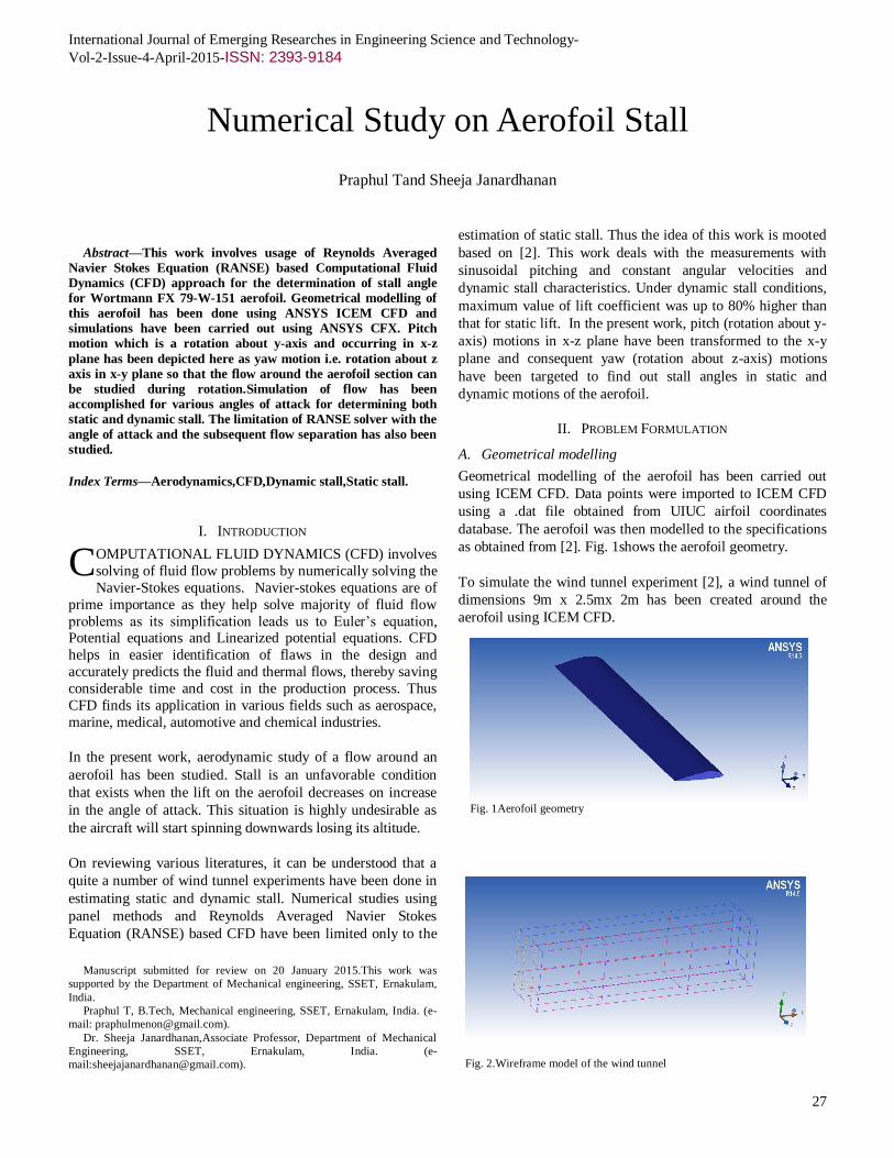
Geometrical modelling of the aerofoil has been carried out
using ICEM CFD. Data points were imported to ICEM CFD
using a .dat file obtained from UIUC airfoil coordinates
database. The aerofoil was then modelled to the specifications
as obtained from [2]. Fig. 1shows the aerofoil geometry.
To simulate the wind tunnel experiment [2], a wind tunnel of
dimensions 9m x 2.5mx 2m has been created around the
aerofoil using ICEM CFD.
Numerical Study on Aerofoil Stall
Praphul Tand Sheeja Janardhanan
C
Fig. 1Aerofoil geometry
Fig. 2.Wireframe model of the wind tunnel
International Journal of Emerging Researches in Engineering Science and Technology-
Vol-2-Issue-4-April-2015-ISSN: 2393-9184
28
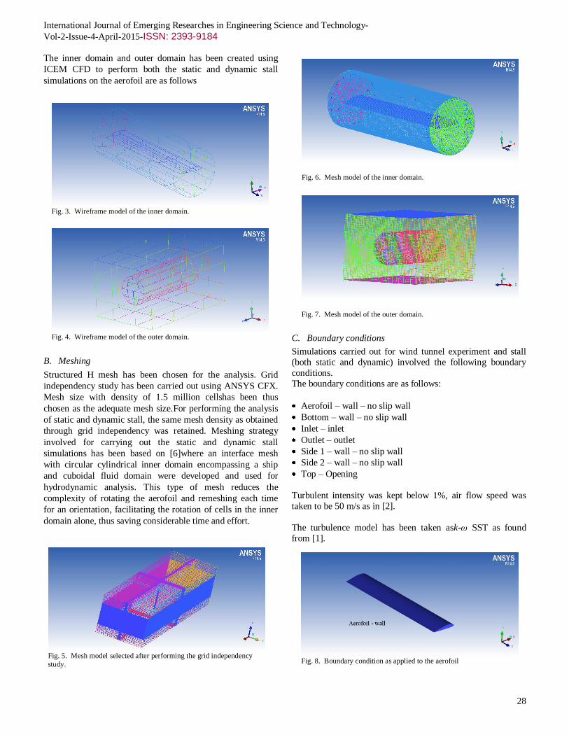
The inner domain and outer domain has been created using
ICEM CFD to perform both the static and dynamic stall
simulations on the aerofoil are as follows
B. Meshing
Structured H mesh has been chosen for the analysis. Grid
independency study has been carried out using ANSYS CFX.
Mesh size with density of 1.5 million cellshas been thus
chosen as the adequate mesh size.For performing the analysis
of static and dynamic stall, the same mesh density as obtained
through grid independency was retained. Meshing strategy
involved for carrying out the static and dynamic stall
simulations has been based on [6]where an interface mesh
with circular cylindrical inner domain encompassing a ship
and cuboidal fluid domain were developed and used for
hydrodynamic analysis. This type of mesh reduces the
complexity of rotating the aerofoil and remeshing each time
for an orientation, facilitating the rotation of cells in the inner
domain alone, thus saving considerable time and effort.
C. Boundary conditions
Simulations carried out for wind tunnel experiment and stall
(both static and dynamic) involved the following boundary
conditions.
The boundary conditions are as follows:
Aerofoil – wall – no slip wall
Bottom – wall – no slip wall
Inlet – inlet
Outlet – outlet
Side 1 – wall – no slip wall
Side 2 – wall – no slip wall
Top – Opening
Turbulent intensity was kept below 1%, air flow speed was
taken to be 50 m/s as in [2].
The turbulence model has been taken ask-ω SST as found
from [1].
Fig. 3. Wireframe model of the inner domain.
Fig. 4. Wireframe model of the outer domain.
Fig. 5. Mesh model selected after performing the grid independency
study.
Fig. 6. Mesh model of the inner domain.
Fig. 7. Mesh model of the outer domain.
Fig. 8. Boundary condition as applied to the aerofoil
International Journal of Emerging Researches in Engineering Science and Technology-
Vol-2-Issue-4-April-2015-ISSN: 2393-9184
29
D. CFD analysis
1) Static stall
Static stall is the stall condition observed for the flow over the
aerofoil at a fixed angle of attack. For static stall estimations,
the inner domain was rotated about the z axis in counter
clockwise as well as clockwise directions for various angles of attack. The various angles of attack under consideration here
are from 0 degree to 15 degree in steps of 2.5 degree
increments for each angle.
2) Dynamic stall
Dynamic stall occurs when there is sudden change in the angle
of attack by the aerofoil. A sinusoidal rotation about z-axis
was given to the inner domain in CFX pre in order to obtain
yaw movement. The sinusoidal function is as follows:
ta sin (1)
= Amplitude of oscillation.
a=Maximum amplitude of oscillation = 0.2618 rad
= Angular frequency of oscillation = 0.5 rad/sec
t = instantaneous time in s
.txt, .xlsx files were written to give inputs to the CFX solver
for interpolating the values. Animation on the dynamic stall
analysis was also performed.
III. RESULTS
A. CFD Validation
Validation of CFD was done by comparing the values of
coefficient of lift obtained for the aerofoil at zero degree of attack between the CFX simulation and the experimental value
obtained from [2]as shown
The values thus are close to each other thus validating the mesh and CFD analysis.
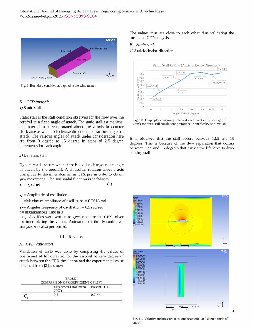
B. Static stall
1) Anticlockwise direction
It is observed that the stall occurs between 12.5 and 15
degrees. This is because of the flow separation that occurs
between 12.5 and 15 degrees that causes the lift force to drop
causing stall.
Fig. 9. Boundary condition as applied to the wind tunnel
Fig. 10. Graph plot comparing values of coefficient of lift vs. angle of
attack for static stall simulations performed in anticlockwise direction.
0, 0.216
2.5, 0.414
5, 0.571
7.5, 0.728
10, 0.92
12.5, 0.95
13.75, 0.896
15, 0.937
0
0.1
0.2
0.3
0.4
0.5
0.6
0.7
0.8
0.9
1
0 2.5 5 7.5 10 12.5 13.75 15
Co
effi
cien
t o
f li
ft (
Cl)
Angle of attack (degrees)
Static Stall in Yaw (Anticlockwise Direction)
TABLE I
COMPARISON OF COEFFICIENT OF LIFT
Experiment (Mohlmann,
2007)
Present CFD
lC
0.2 0.2144
Fig. 11. Velocity and pressure plots on the aerofoil at 0 degree angle of
attack.
International Journal of Emerging Researches in Engineering Science and Technology-
Vol-2-Issue-4-April-2015-ISSN: 2393-9184
30
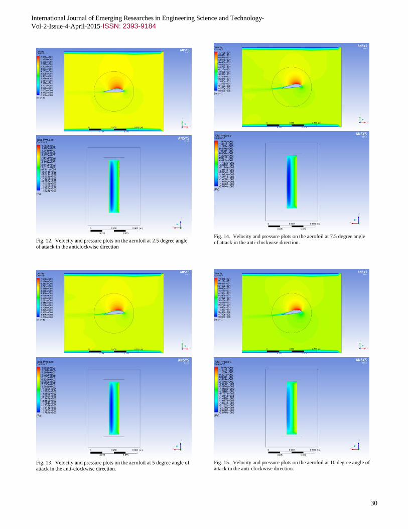
Fig. 13. Velocity and pressure plots on the aerofoil at 5 degree angle of
attack in the anti-clockwise direction.
Fig. 14. Velocity and pressure plots on the aerofoil at 7.5 degree angle
of attack in the anti-clockwise direction.
Fig. 12. Velocity and pressure plots on the aerofoil at 2.5 degree angle
of attack in the anticlockwise direction
Fig. 15. Velocity and pressure plots on the aerofoil at 10 degree angle of
attack in the anti-clockwise direction.
International Journal of Emerging Researches in Engineering Science and Technology-
Vol-2-Issue-4-April-2015-ISSN: 2393-9184
31
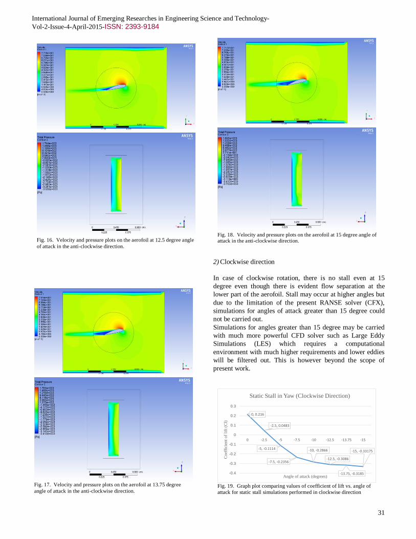
2) Clockwise direction
In case of clockwise rotation, there is no stall even at 15
degree even though there is evident flow separation at the
lower part of the aerofoil. Stall may occur at higher angles but
due to the limitation of the present RANSE solver (CFX),
simulations for angles of attack greater than 15 degree could
not be carried out.
Simulations for angles greater than 15 degree may be carried
with much more powerful CFD solver such as Large Eddy
Simulations (LES) which requires a computational
environment with much higher requirements and lower eddies
will be filtered out. This is however beyond the scope of
present work.
Fig. 18. Velocity and pressure plots on the aerofoil at 15 degree angle of attack in the anti-clockwise direction.
Fig. 16. Velocity and pressure plots on the aerofoil at 12.5 degree angle
of attack in the anti-clockwise direction.
Fig. 17. Velocity and pressure plots on the aerofoil at 13.75 degree
angle of attack in the anti-clockwise direction.
Fig. 19. Graph plot comparing values of coefficient of lift vs. angle of
attack for static stall simulations performed in clockwise direction
0, 0.216
-2.5, 0.0483
-5, -0.1114
-7.5, -0.2356
-10, -0.2866
-12.5, -0.3086
-13.75, -0.3185
-15, -0.33175
-0.4
-0.3
-0.2
-0.1
0
0.1
0.2
0.3
0 -2.5 -5 -7.5 -10 -12.5 -13.75 -15
Co
effi
cien
t o
f li
ft (
Cl)
Angle of attack (degrees)
Static Stall in Yaw (Clockwise Direction)
International Journal of Emerging Researches in Engineering Science and Technology-
Vol-2-Issue-4-April-2015-ISSN: 2393-9184
32
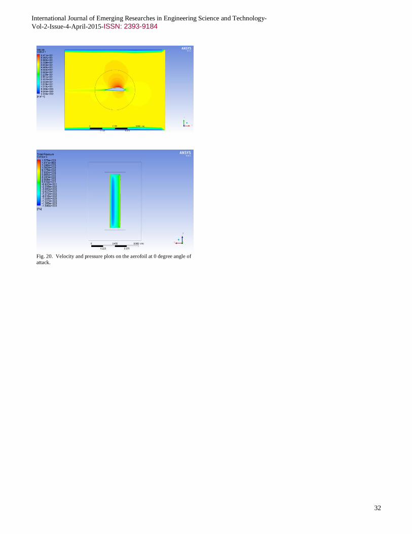
Fig. 20. Velocity and pressure plots on the aerofoil at 0 degree angle of
attack.
International Journal of Emerging Researches in Engineering Science and Technology-
Vol-2-Issue-4-April-2015-ISSN: 2393-9184
33
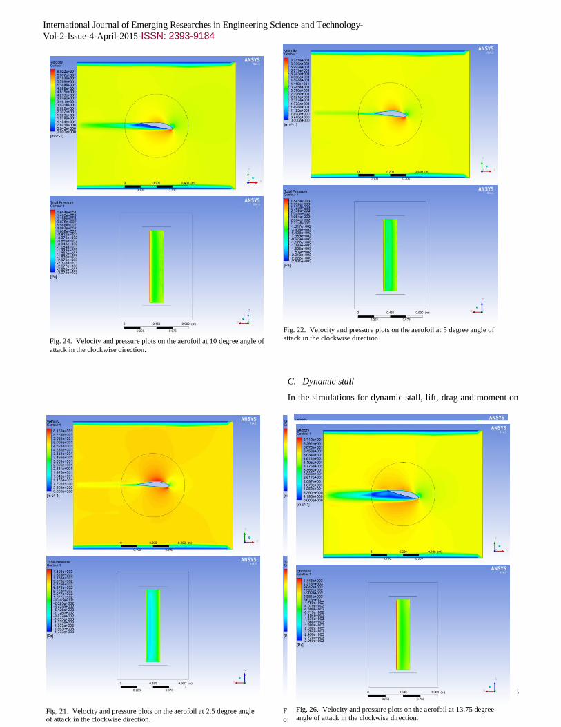
C. Dynamic stall
In the simulations for dynamic stall, lift, drag and moment on
Fig. 27. Velocity and pressure plots on the aerofoil at 15 degree angle of
attack in the clockwise direction.
Fig. 22. Velocity and pressure plots on the aerofoil at 5 degree angle of attack in the clockwise direction.
Fig. 21. Velocity and pressure plots on the aerofoil at 2.5 degree angle of attack in the clockwise direction.
Fig. 23. Velocity and pressure plots on the aerofoil at 7.5 degree angle
of attack in the clockwise direction.
Fig. 24. Velocity and pressure plots on the aerofoil at 10 degree angle of
attack in the clockwise direction.
Fig. 25. Velocity and pressure plots on the aerofoil at 12.5 degree angle
of attack in the clockwise direction.
Fig. 26. Velocity and pressure plots on the aerofoil at 13.75 degree
angle of attack in the clockwise direction.
International Journal of Emerging Researches in Engineering Science and Technology-
Vol-2-Issue-4-April-2015-ISSN: 2393-9184
34
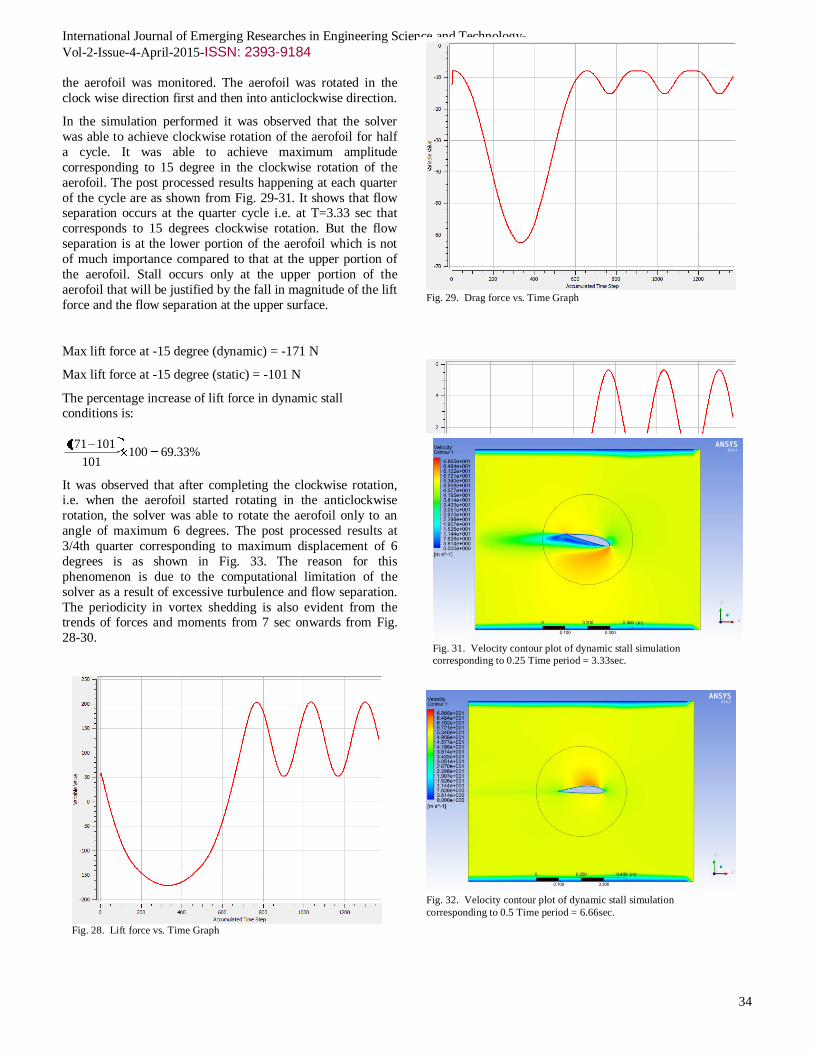
the aerofoil was monitored. The aerofoil was rotated in the
clock wise direction first and then into anticlockwise direction.
In the simulation performed it was observed that the solver
was able to achieve clockwise rotation of the aerofoil for half
a cycle. It was able to achieve maximum amplitude
corresponding to 15 degree in the clockwise rotation of the
aerofoil. The post processed results happening at each quarter
of the cycle are as shown from Fig. 29-31. It shows that flow separation occurs at the quarter cycle i.e. at T=3.33 sec that
corresponds to 15 degrees clockwise rotation. But the flow
separation is at the lower portion of the aerofoil which is not
of much importance compared to that at the upper portion of
the aerofoil. Stall occurs only at the upper portion of the
aerofoil that will be justified by the fall in magnitude of the lift
force and the flow separation at the upper surface.
Max lift force at -15 degree (dynamic) = -171 N
Max lift force at -15 degree (static) = -101 N
The percentage increase of lift force in dynamic stall conditions is:
%33.69100101
101171
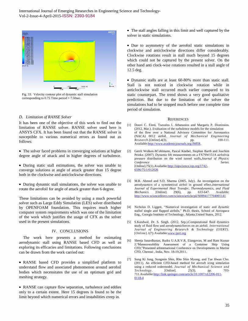
It was observed that after completing the clockwise rotation, i.e. when the aerofoil started rotating in the anticlockwise
rotation, the solver was able to rotate the aerofoil only to an
angle of maximum 6 degrees. The post processed results at
3/4th quarter corresponding to maximum displacement of 6
degrees is as shown in Fig. 33. The reason for this
phenomenon is due to the computational limitation of the
solver as a result of excessive turbulence and flow separation.
The periodicity in vortex shedding is also evident from the trends of forces and moments from 7 sec onwards from Fig.
28-30.
Fig. 32. Velocity contour plot of dynamic stall simulation
corresponding to 0.5 Time period = 6.66sec.
Fig. 28. Lift force vs. Time Graph
Fig. 29. Drag force vs. Time Graph
Fig. 30. Moment vs. Time Graph
Fig. 31. Velocity contour plot of dynamic stall simulation
corresponding to 0.25 Time period = 3.33sec.
International Journal of Emerging Researches in Engineering Science and Technology-
Vol-2-Issue-4-April-2015-ISSN: 2393-9184
35
D. Limitation of RANSE Solver
It has been one of the objective of this work to find out the
limitation of RANSE solver. RANSE solver used here is
ANSYS CFX. It has been found out that the RANSE solver is
susceptible to various numerical errors as found out as
follows:
The solver faced problems in converging solutions at higher
degree angle of attack and in higher degrees of turbulence.
During static stall estimations, the solver was unable to
converge solutions at angle of attack greater than 15 degree
both in the clockwise and anticlockwise directions.
During dynamic stall simulations, the solver was unable to
rotate the aerofoil for angle of attack greater than 6 degree.
These limitations can be avoided by using a much powerful solver such as Large Eddy Simulation (LES) solver distributed
by OPENFOAM foundation. This requires much higher
computer system requirements which was one of the limitation
of the work which justifies the usage of CFX as the solver
used in the present simulations.
IV. CONCLUSIONS
The work here presents a method for estimating
aerodynamic stall using RANSE based CFD as well as
exploring its efficacies and limitations. Following conclusions
can be drawn from the work carried out:
RANSE based CFD provides a simplified platform to
understand flow and associated phenomenon around aerofoil
bodies which necessitates the use of an optimum grid and
meshing strategy.
RANSE can capture flow separation, turbulence and eddies
only to a certain extent. Here 15 degrees is found to be the
limit beyond which numerical errors and instabilities creep in.
The stall angles falling in this limit and well captured by the
solver in static simulations.
Due to asymmetry of the aerofoil static simulations in
clockwise and anticlockwise directions differ considerably.
Clockwise rotations result in stall much beyond 15 degrees
which could not be captured by the present solver. On the
other hand anti clock-wise rotations resulted in a stall angle of
12.5 deg.
Dynamic stalls are at least 60-80% more than static stall.
Stall is not noticed in clockwise rotation while in
anticlockwise stall occurred much earlier compared to its
static counterpart. The trend shows a very good qualitative
prediction. But due to the limitation of the solver the
simulations had to be stopped much before one complete time
period of simulation.
REFERENCES
[1] Douvi C. Eleni, Tsavalos I. Athanasios and Margaris P. Dionissios.
(2012, Mar.). Evaluation of the turbulence models for the simulation
of the flow over a National Advisory Committee for Aeronautics
(NACA) 0012 airfoil. Journal of Mechanical Engineering
Research.[Online].4(3), pp. 100-111.
Available:http://www.academicjournals.org/JMER.
[2] Gerrit Wolken-M¨ohlmann, Pascal Knebel, Stephan Barth and Joachim
Peinke. (2007) .Dynamic lift measurements on a FX79W151A airfoilvia
pressure distribution on the wind tunnel walls,Journal of Physics:
Conference Series.
[Online].75(1),Available:http://iopscience.iop.org/1742-
6596/75/1/012026
[3] M.R. Ahmed and S.D. Sharma (2005, July). An investigation on the
aerodynamics of a symmetrical airfoil in ground effect,International
Journal of Experimental Heat Transfer, Thermodynamics, and Fluid
Mechanics. [Online]. 29(6), pp. 633-647. Available:
http://www.sciencedirect.com/science/article/pii/S0894177704001141
[4] Nicholas D. Liggett, “Numerical investigation of static and dynamic
stallof single and flapped airfoils,” Ph.D. thesis, School of Aerospace
Eng., Georgia Institute of Technology, Atlanta,United States, 2012.
[5] S.Kandwal, Dr. S. Singh. (2012, Sep.).Computational fluid dynamics
study of fluid flow and aerodynamicforces on an airfoil. International
Journal of Engineering Research & Technology (IJERT).
[Online].1(7).Available:www.ijert.org
[6] Sheeja Janardhanan, Rudra U.A.R.V.R, Elangovan, M and Ram Kumar
J,“Maneuverability Assessment of a Container Ship Using
CFD,”Presented atInternational Conference on Developments in Marine
CFD, Chennai , India, Nov. 18-19,2011.
[7] Sung Ki Jung, Sungmin Shin, Rho Shin Myong, and Tae Hwan Cho.
(2011). An efficient CFD-based method for aircraft icing simulation
using a reduced ordermodel. Journal of Mechanical Science and
Technology. [Online]. 25(3), pp. 703-
711.Available:http://link.springer.com/article/10.1007/s12206-011-
0118-4
Fig. 33. Velocity contour plot of dynamic stall simulation
corresponding to 0.75 Time period = 7.50sec.