numerical weather prediction parametrization of diabatic processes clouds (4) cloud scheme...

Numerical Weather Prediction Numerical Weather Prediction Parametrization of diabatic Parametrization of diabatic

processesprocesses

Clouds (4)Clouds (4)Cloud Scheme ValidationCloud Scheme Validation

Richard Forbes and Adrian Tompkins [email protected]

RICH,

AN ECMWFLECTURER

2

Cloud Validation: The issuesCloud Validation: The issues

• AIM: To perfectly simulate one aspect of nature: CLOUDS

• APPROACH: Validate the model generated clouds against observations, and use the information concerning apparent errors to improve the model physics, and subsequently the cloud simulation.

Cloud observations

Cloud simulation

error parameterisation

improvements

sounds easy?

3

Cloud Validation: The Cloud Validation: The problemsproblems

• How much of the ‘error’ derives from observations?

Cloud observations error = 1

Cloud simulation error = 2


improvements

4

Cloud Validation: The Cloud Validation: The problemsproblems

• Which Physics is responsible for the error?

Cloud observations

Cloud simulation


improvements

radiation

convectioncloud

physicsdynamics

turbulence

5

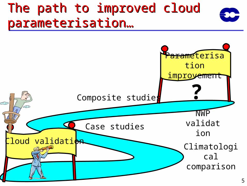
The path to improved cloud The path to improved cloud parameterisation…parameterisation…

Cloud validation

Parameterisation improvement

Climatological comparison

Case studies

Composite studies

NWP validation

?

ECMWF Model Configurations

• ECMWF Global Atmospheric Model (IFS) • Many different configurations at different resolutions:

TL159 (125 km) L62 Seasonal Forecast System (→6 months)

TL255 (80 km) L62 Monthly Forecast System (→32 days)

TL399 (50 km) L62 Ensemble Prediction System (EPS) (→15 days)

TL799 (25 km) L91 Current Deterministic Global NWP (→10 days)

TL1279 (16 km) L91 NWP from 2009 (→10 days)

Future: 150 levels (Δ250m@z=5km)? 10 km horizontal resolution?..........

• Need verification across a range of spatial scales and timescales → a model with a “climate” that is robust to resolution.

7

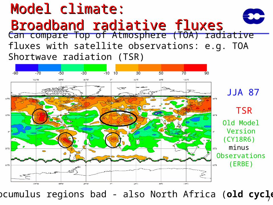
Model climate: Model climate: Broadband radiative fluxesBroadband radiative fluxes

JJA 87

TSR

Stratocumulus regions bad - also North Africa (old cycle!)

Can compare Top of Atmosphere (TOA) radiative fluxes with satellite observations: e.g. TOA Shortwave radiation (TSR)

Old Model Version(CY18R6)

minus Observations

(ERBE)

8

Model climate:Model climate:Cloud radiative “forcing”Cloud radiative “forcing”

• Problem: Can we associate these “errors” with clouds?• Another approach is to examine “cloud radiative forcing”

Note CRF sometimes defined as Fclr-F, also differences in model calculation

JJA 87

SWCRF

Cloud Problems: strato-cu YES, North Africa NO!


minus Observations

(ERBE)

9

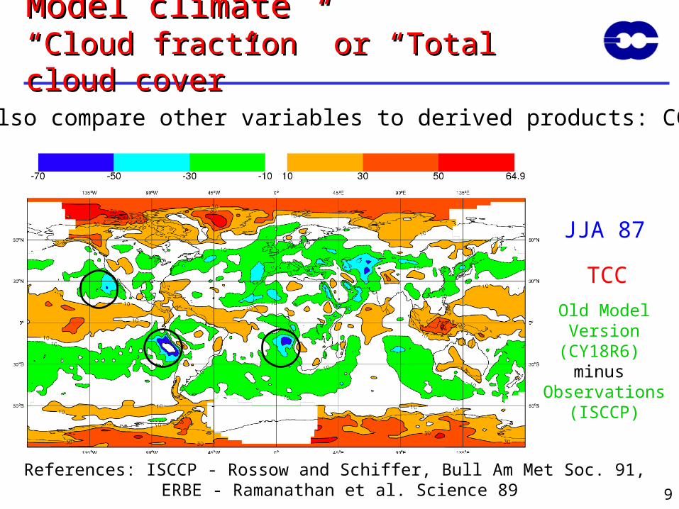
Model climateModel climate“Cloud fraction” or “Total cloud “Cloud fraction” or “Total cloud cover”cover”

JJA 87

TCC

References: ISCCP - Rossow and Schiffer, Bull Am Met Soc. 91, ERBE - Ramanathan et al. Science 89

Can also compare other variables to derived products: CC


minus Observations

(ISCCP)

10

Comparison with Satellite Comparison with Satellite Data: Data: A problemA problem

If more complicated cloud parameters are desired (e.g. vertical structure) then retrieval can be ambiguous

Channel 1 Channel 2 …..

Liquid cloud 1

Liquid cloud 2

Liquid cloud 3

Ice cloud 1

Ice cloud 2

Ice cloud 3

Vapour 1

Vapour 2

Vapour 3Hei

ght

Ass

um

pti

on

s ab

ou

t ve

rtic

al

stru

ctu

res Another approach is to

simulate irradiances using model fields

Rad

iati

ve

tran

sfer

m

od

el

11

Comparison with Satellite Comparison with Satellite Data:Data:Simulating Satellite RadiancesSimulating Satellite Radiances

Examples: Morcrette MWR 1991, Chevallier et al, J Clim. 2001

More certainty in the diagnosis of the existence of a problem. Doesn’t necessarily help identify the origin of the problem

70°S 70°S

60°S60°S

50°S 50°S

40°S40°S

30°S 30°S

20°S20°S

10°S 10°S

0°0°

10°N 10°N

20°N20°N

30°N 30°N

40°N40°N

50°N 50°N

60°N60°N

70°N 70°N

60°W 40°W 20°W 0° 20°E 40°E 60°E

METEOSAT 7 First Infrared Band Monday 11 April 2005 0600UTC

70°S 70°S

60°S60°S

50°S 50°S

40°S40°S

30°S 30°S

20°S20°S

10°S 10°S

0°0°

10°N 10°N

20°N20°N

30°N 30°N

40°N40°N

50°N 50°N

60°N60°N

70°N 70°N

60°W 40°W 20°W 0° 20°E 40°E 60°E

RTTOV generated METEOSAT 7 First Inf rared Band (10 bit)Sunday 10 April 2005 12UTC ECMWF Forecast t+18 VT:Monday 11 April 2005 06UTC

12

Comparison with Satellite Data:Comparison with Satellite Data:A more complicated analysis is A more complicated analysis is possible…possible…

DIURNAL CYCLEOVER TROPICAL

LAND

VARIABILITY

Observations:late afternoon peak in

convection

Model: morning peak

(Common problem)

13

NWP Forecast EvaluationNWP Forecast Evaluation

• Differences in longer simulations may not be the direct result of the cloud scheme– Interaction with radiation, dynamics etc.– E.g: poor stratocumulus regions

• Using short-term NWP or analysis restricts this and allows one to concentrate on the cloud scheme

Introduction of Tiedtke Scheme

Time

Cloud cover bias

14

Example over EuropeExample over Europe

30°N

35°N

40°N

45°N

50°N

55°N

60°N

65°N

70°N

50°W

50°W

40°W

40°W

30°W

30°W

20°W

20°W

10°W

10°W

0°

0°

10°E

10°E

20°E

20°E

30°E

30°E 40°E

40°E

50°E

50°E

60°E

60°E

70°E70°E

N= 10761 BIAS= -0.55 STDEV= 2.61 MAE= 1.91FC PERIOD: 20050401 - 20050412 STEP: 48 VALID AT: 12 UTC

BIAS Total Cloud Cover [octa] ECM

-8 - -3 -3 - -1 -1 - 1 1 - 3 3 - 8-1:1 1:3 3:8-3:-1-8:-3

15

20°N

25°N

30°N

35°N

40°N

45°N

50°N

55°N

60°N

65°N

50°W

50°W

45°W

45°W

40°W

40°W

35°W

35°W

30°W

30°W

25°W

25°W

20°W

20°W

15°W

15°W

10°W

10°W

5°W

5°W

0°

0°

5°E

5°E

10°E

10°E

15°E

15°E

20°E

20°E

25°E

25°E

30°E

30°E35°E

35°E

40°E

40°E

45°E

45°E

50°E

50°E

55°E

55°E

60°E

60°E

65°E

65°E

METEOSAT 7 First Infrared Band Monday 11 April 2005 1200UTC

20°N

25°N

30°N

35°N

40°N

45°N

50°N

55°N

60°N

65°N

50°W

50°W

45°W

45°W

40°W

40°W

35°W

35°W

30°W

30°W

25°W

25°W

20°W

20°W

15°W

15°W

10°W

10°W

5°W

5°W

0°

0°

5°E

5°E

10°E

10°E

15°E

15°E

20°E

20°E

25°E

25°E

30°E

30°E35°E

35°E

40°E

40°E

45°E

45°E

50°E

50°E

55°E

55°E

60°E

60°E

65°E

65°E

RTTOV generated METEOSAT 7 First Inf rared Band (10 bit)Sunday 10 April 2005 12UTC ECMWF Forecast t+24 VT:Monday 11 April 2005 12UTC

Daily Report 11Daily Report 11thth April 2005 April 2005

“Going more into details of the cyclone, it can be seen that the model was able to reproduce the very peculiar spiral structure in the clouds bands. However large differences can be noticed further east, in the warm sector of the frontal system attached to the

cyclone, where the model largely underpredicts the typical high-cloud shield. Look for example in the two maps above where a clear deficiency of cloud cover is evident in the model generated satellite images north of the Black Sea. In this case this was systematic

over different forecasts.” – Quote from ECMWF daily report 11th April 2005

NWP Forecast EvaluationNWP Forecast EvaluationMeteosat and simulated IRMeteosat and simulated IR

16

METEOSAT 7 Water Vapour Band Monday 11 April 2005 2000UTC RTTOV generated METEOSAT 7 Water Vapour Band (10 bit)Sunday 10 April 2005 12UTC ECMWF Forecast t+30 VT:Monday 11 April 2005 18UTC

Blue: moistRed: Dry

30 hr forecast too dry in front regionIs not a FC-drift, does this mean the cloud scheme is at fault?

NWP Forecast EvaluationNWP Forecast EvaluationMeteosat and simulated w.v. channelMeteosat and simulated w.v. channel

17

Case StudiesCase Studies

• Can concentrate on a particular location and/or time period in more detail, for which specific observational data is collected:

CASE STUDY

• Examples: – GATE, CEPEX, TOGA-COARE, ARM...

18

Evaluation of vertical cloud Evaluation of vertical cloud structurestructure

Mace et al., 1998, GRL

Examined the frequency of occurrence of ice cloud

Reasonable match to data found

ARM Site - America Great Plains

19

Evaluation of vertical cloud Evaluation of vertical cloud structurestructure

Hogan et al., 2001, JAM

Analysis using the radar and lidar at Chilbolton, UK.

Reasonable Match

20

Hogan et al. More details Hogan et al. More details possiblepossible

21

Hogan et al. Hogan et al. (2001)(2001)

Comparison improved when:

(a) snow was included,

(b) cloud below the sensitivity of the instruments was removed.

22

Issues Raised:Issues Raised:

• WHAT ARE WE COMPARING?– Is the model statistic really equivalent to what the

instrument measures?– e.g: Radar sees snow, but the model may not include this in

the definition of cloud fraction. Small ice amounts may be invisible to the instrument but included in the model statistic

• HOW STRINGENT IS OUR TEST? – Perhaps the variable is easy to reproduce– e.g: Mid-latitude frontal clouds are strongly dynamically

forced, cloud fraction is often zero or one. Perhaps cloud fraction statistics are easy to reproduce in short term forecasts

23

Can also use to validate Can also use to validate “components” of cloud “components” of cloud schemescheme

EXAMPLE: Cloud Overlap AssumptionsHogan and Illingworth, 2000,

QJRMS

Issues Raised: HOW REPRESENTATIVE IS OUR CASE STUDY LOCATION?e.g: Wind shear and dynamics very different between Southern England and the tropics!!!

24

CompositesComposites

• We want to look at a certain kind of model system: – Stratocumulus regions– Extra tropical cyclones

• An individual case may not be conclusive: Is it typical?

• On the other hand general statistics may swamp this kind of system

• Can use compositing technique

25

Composites - a cloud surveyComposites - a cloud survey

Tselioudis et al., 2000, JCL

From Satellite attempt to derive

cloud top pressure and cloud optical

thickness for each pixel - Data is then

divided into regimes according

to sea level pressure anomaly

Use ISCCP simulator

1. High Clouds too thin

2. Low clouds too thick

Data Model Modal-Data

Optical depth

Clo

ud t

op p

ress

ure

1.

2.

900

500

620

750

350

250

120

-ve

SLP

900

500

620

750

350

250

120

+ve

SLP

26

Composites – Extra-tropical Composites – Extra-tropical cyclonescyclones

Overlay about 1000 cyclones, defined about a location of maximum optical thickness

Plot predominant cloud types by looking at anomalies from 5-day average

Klein and Jakob, 1999, MWR

High tops=Red, Mid tops=Yellow, Low tops=Blue

• High Clouds too thin

• Low clouds too thick

27

A strategy for cloud A strategy for cloud parametrization evaluationparametrization evaluation

Jakob

28

Recap: The problemsRecap: The problems

• All Observations– Are we comparing ‘like with like’? What assumptions are contained

in retrievals/variational approaches?

• Long term climatologies:– Which physics is responsible for the errors?– Dynamical regimes can diverge

• NWP, Reanalysis, Column Models– Doesn’t allow the interaction between physics to be represented

• Case studies– Are they representative? Do changes translate into global skill?

• Composites As case studies.

• And one more problem specific to NWP…

29

NWP cloud scheme developmentNWP cloud scheme development

Timescale of validation exercise– Many of the above validation exercises are complex and

involved– Often the results are available O(years) after the project

starts for a single version of the model– ECMWF operational model is updated 2 to 4 times a

year roughly, so often the validation results are no longer relevant, once they become available.

RequirementRequirement: A quick and easy test bench

30

Example: LWP ERA-40 and recent Example: LWP ERA-40 and recent cyclescycles

23r4: June 2001 26r1: April 2003

mod

elS

SM

ID

iff

31


23r4: June 2001 26r3: Oct 2003

mod

elS

SM

ID

iff

32


23r4: June 2001 28r1: Mar 2004

mod

elS

SM

ID

iff

33


23r4: June 2001 28r3: Sept 2004

mod

elS

SM

ID

iff

34


23r4: June 2001 29r1: Apr 2005

mod

elS

SM

ID

iff

35


23r4: June 2001 33r1: Nov 2008

Do ERA-40 cloud studies still have relevance for the operational model?

mod

elS

SM

ID

iff

36

So what do we use at ECMWF?So what do we use at ECMWF?

• T799-L91– Standard

“Scores” (rms, anom corr of U, T, Z)

– “operational” validation of clouds against SYNOP observations

– Simulated radiances against Meteosat 7

• T159-L91 – “climate” runs– 4 ensemble members of 13 months– Automatically produces comparisons to:

• ERBE, NOAA-x, CERES TOA fluxes• Quikscat & SSM/I, 10m winds• ISCCP & MODIS cloud cover• SSM/I, TRMM liquid water path• (soon MLS ice water content)• GPCP, TRMM, SSM/I, Xie Arkin, Precip• Dasilva climatology of surface fluxes• ERA-40 analysis winds

37

Ease of use allows catalogue of climate

to be built up

Issues

1.Obs errors

2.Variance

3.Resolution sensitivity

38

Top-of-Top-of-atmos net atmos net

LW LW radiationradiation

Model T159 L91

CERES

Difference

too high

too low

-150

-300

-150

-300

39

Model T159 L91

CERES

Difference

albedo high

albedo low

350

100

350

100

Top-of-Top-of-atmos net atmos net

SW SW radiationradiation

40

Total Cloud Total Cloud Cover Cover (TCC) (TCC)

Model T159 L91

ISCCP

Difference

TCC high

TCC low

80

10

80

10

41

Total Total Column Column Liquid Liquid WaterWater

(TCLW) (TCLW)

Model T159 L91

SSMI

Difference

high

low

250

25

250

25

42

Model validationModel validationLook at higher order statistics

Example: PDF of cloud cover

Highlights a problem with one particular model version!

43

Model validationModel validationLook at relationships between variables

Example: Liquid water path versus probability of precipitation for different precipitation thresholds

Can compare with satellite observations of LWP and precipitation rate → autoconversion parametrization

44

Model validationModel validationMaking the most of instrument synergy

• Observational instruments measure one aspect of the atmosphere.

• Often, combining information from different instruments can provide complementary information (particularly for remote sensing)

• For example, radars at different wavelengths, lidar, radiometers. Radar, lidar and

radiometer instruments at Chilbolton, UK

(www.chilbolton.rl.ac.uk)

45

Long term ground-based Long term ground-based observations ARM / CLOUDNETobservations ARM / CLOUDNET

• Network of stations processed for multi-year period using identical algorithms, first Europe, now also ARM sites

• Some European provide operational forecasts so that direct comparisons are made quasi-realtime

• Direct involvement of Met services to provide up-to-date information on model cycles

46

Long term ground-based Long term ground-based observations observations ARM Observational Sites

• “Permanent” ARM sites and movable “ARM mobile facility” for observational campaigns.

47

Cloudnet ExampleCloudnet Example

• In addition to standard quicklooks, longer-term statistics are available

• This example is for ECMWF cloud cover during June 2005

• Includes preprocessing to account for radar attenuation and snow

• See www.cloud-net.org for more details and examples! (but not funded at the current time !)

48

Space-borne active remote Space-borne active remote sensingsensingA-Train

• CloudSat and CALIPSO have active radar and lidar to provide information on the vertical profile of clouds and precipitation. (Launched 28th April 2006)

• Approaches to model validation:

Model → Obs parameters

Obs → Model parameters

Model Data(T,p,q,iwc,lwc…)

Sub-grid Cloud/Precip

Pre-processor

CloudSat simulator (Haynes et al. 2007)

CALIPSO simulator (Chiriaco et al. 2006)

Lidar Attenuated Backscatter

Radar Reflectivity

Physical Assumptions

(PSDs, Mie tables...)

Simulating ObservationsCFMIP COSP radar/lidar simulator

50

Example cross-section through a Example cross-section through a frontfrontModel vs CloudSat radar reflectivityModel vs CloudSat radar reflectivity

51

Example CloudSat orbit “quicklook”Example CloudSat orbit “quicklook”http://www.cloudsat.cira.colostate.edu/dpcstatusQL.phhttp://www.cloudsat.cira.colostate.edu/dpcstatusQL.phpp

52

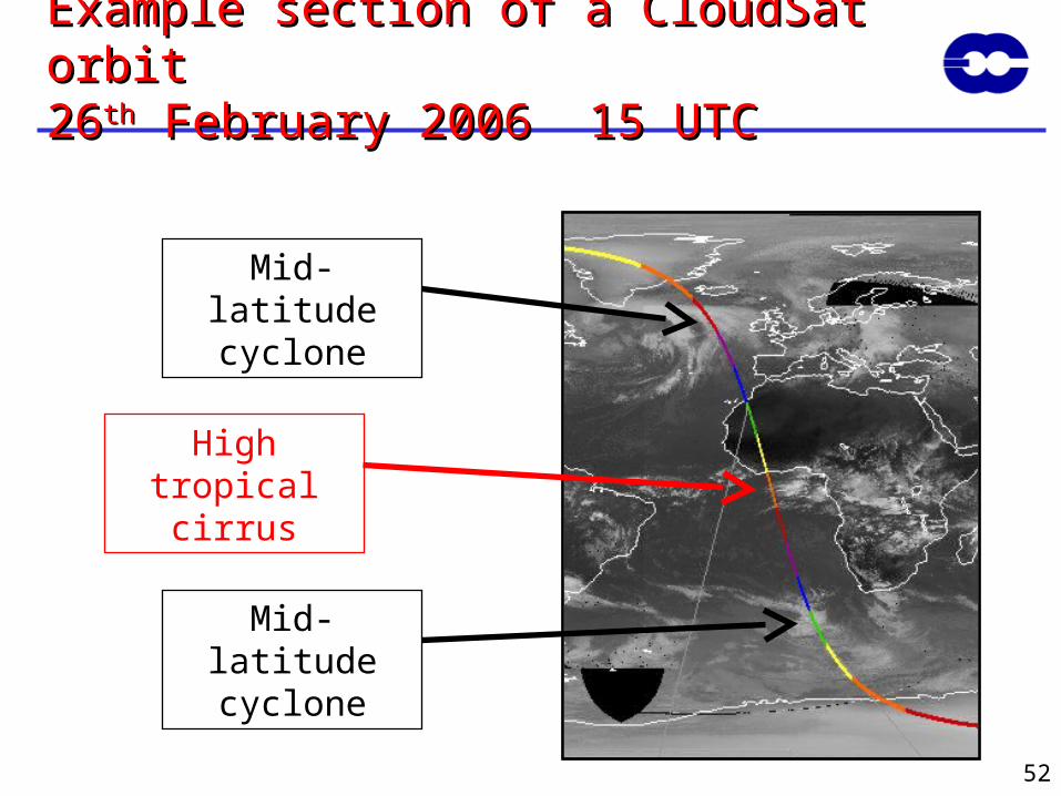
Example section of a CloudSat Example section of a CloudSat orbitorbit2626thth February 2006 15 UTC February 2006 15 UTC

Mid-latitude cyclone

High tropical cirrus

Mid-latitude cyclone

53

Compare model with observed Compare model with observed parameters: Radar reflectivityparameters: Radar reflectivity

Simulated radar reflectivity from the model.

(ice only)

Observed radar reflectivity from CloudSat

(ice + rain)

Tropics 82°N82°S

0°C

0°C

26/02/2007 15Z

54

Compare model parameters with Compare model parameters with equivalent derived from observations: equivalent derived from observations: Ice AmountIce Amount

Model ice water content (excluding precipitating snow).

Ice water content derived from a

1DVAR retrieval of CloudSat/

CALIPSO/Aqua

log10

kg m-3

(Delanöe and Hogan (2007), Reading Univ., UK)

Eq EqEq GreenlandAntarctica

26/02/2007 15Z

Summary

• Different approaches to verification (climate statistics, case studies, composites), different techniques (model-to-obs, obs-to-model) and a range of observations are required to validate and improve cloud parametrizations.

• Need to understand the limitations of observational data (e.g. what is beyond the senistivity limits of the radar, or what is the accuracy of derived liquid water path from satellite)

• The model developer needs to understand physical processes to improve the model. Usually this requires observations, theory and modelling, but observations can be used to test model’s physical relationships between variables.

56


Cloud validation


Case studies

Composite studies

NWP validation

?


57


Cloud validation


Case studies

Composite studies

NWP validation

?Many mountains to climb !


numerical weather prediction parametrization of diabatic processes clouds (4) cloud scheme...

Documents