numerische mathematik - cscamm · numer. math. (1998) 79: 397–425 numerische mathematik c...

Numer. Math. (1998) 79: 397–425 NumerischeMathematikc© Springer-Verlag 1998

Electronic Edition

Third order nonoscillatory central schemefor hyperbolic conservation laws

Xu-Dong Liu1, Eitan Tadmor2,3

1 Department of Mathematics, UCSB, Santa Barbara, CA 93106, USA; e-mail: [email protected] School of Mathematical Sciences, Tel-Aviv University, Tel-Aviv 69978, Israel3 Department of Mathematics, UCLA, Los Angeles CA 90095, USA;

e-mail: [email protected]

Received April 10, 1996 / Revised version received January 20, 1997

Summary. A third-order accurate Godunov-type scheme for the approxi-mate solution of hyperbolic systems of conservation laws is presented. Itstwo main ingredients include: 1. A non-oscillatory piecewise-quadratic re-construction of pointvalues from their given cell averages; and 2. A centraldifferencing based onstaggeredevolution of the reconstructed cell aver-ages. This results in a third-order central scheme, an extension along thelines of the second-order central scheme of Nessyahu and Tadmor [NT].The scalar scheme is non-oscillatory (and hence – convergent), in the sensethat it does not increase thenumberof initial extrema (– as does the exactentropy solution operator). Extension to systems is carried out bycompo-nentwiseapplication of the scalar framework. In particular, we have theadvantage that, unlike upwind schemes, no (approximate) Riemann solvers,field-by-field characteristic decompositions, etc., are required. Numericalexperiments confirm the high-resolution content of the proposed scheme.Thus, a considerable amount of simplicity and robustness is gained whileretaining the expected third-order resolution.

Mathematics Subject Classification (1991):65M10; 65M05

1 Introduction

In this paper we present a third-order, non-oscillatory central differencescheme for the approximate solution of nonlinear systems of hyperbolicconservation laws. The scheme can be viewed as natural next step in the

Correspondence to: E. Tadmor

Numerische Mathematik Electronic Editionpage 397 of Numer. Math. (1998) 79: 397–425

398 X.-D. Liu, E. Tadmor

sequel to the first-order Lax-Friedrichs(LxF) scheme, and the second-ordercentral scheme of Nessyahu and Tadmor, [NT]. Our third-order schemeenjoys a major advantage of the central schemes over the upwind ones, inthat no Riemann solvers are involved. The use of third-order piecewise-quadratic approximation compensates for the excessive viscosity typical tothe first-order LxF piecewise-constant solution, and it offers an improvedresolution beyond the second-order piecewise-linear approximation used in[NT]. The result is a simple, robust, Riemann-solver-free central differencescheme with third-order resolution.

In Sect. 2, we provide a self-contained discussion on Godunov-typeschemes. Such schemes are based on piecewise-polynomialreconstruction–reconstruction of pointvalues from cell averages, followed by anevolutionstep – the evolution of approximate fluxes. Our point of view is that thedistinction between upwind and central Godunov-type schemes, lies in theway they realize the evolution of these piecewise-polynomials: Upwindschemes sample the reconstructed values at themid-cells; central schemesare based onstaggeredsampling at the interfacingbreakpoints.

In Sect. 3, we recall the non-oscillatory third-order accurate reconstruc-tion due to Liu and Osher [LO], and combine it with central differenc-ing, based onstaggeredsampling along the lines of [NT]. Thus, at eachtime-level, we reconstruct from the given cell-averages, a non-oscillatorypiecewise-quadratic approximation of third-order accuracy. We then followthe evolving solution to the next time level, and end up by projecting backthe staggered cell-averages of the solution.

In Sect. 4 we take a closer look at the non-oscillatory character of ourscalar third-order scheme, proving it is non-oscillatory in the sense of sat-isfying the Number of Extrema Diminishing (NED) property; this, togetherwith an L∞-bound imply the total-variation boundedness and hence theconvergence of the third-order approximate solution.

Finally, in Sect. 5 we present numerical experiments with our third-order, non-oscillatory central difference scheme. Both the quantitative andqualitative results for a representative sample of compressible flow problemsgoverned by Euler equations, are found to be in complete agreement withthe high resolution expected by the scalar analysis. Taking into accountthe ease of implementation, robustness and time performance, these resultscompare favorably with the results obtained by the corresponding upwind-based schemes. Similar results regarding the advantages ofcentral overupwindschemes in robustness, efficiency and simplicity, were concludedby e.g., Sanders, [Sa1],[Sa2], and Huynh, [Hu], and were further amplifiedby our numerical experiments in the forthcoming [JT], [TW].

We conclude this Introduction with a brief overview of previous work onnon-oscillatory schemes of third-order accuracy. The first pioneering work


Third order nonoscillatory central scheme for hyperbolic conservation laws 399

in this category is due to Colella and Woodward, [CW]. Their PPM method,as well as the third-order versions of the ENO scheme, [HEOC], [Sh], in-tegrate a co-monotonicity constrained piecewise-parabolic reconstructioninto the framework ofupwindGodunov-type scheme. Sanders [Sa1], andSanders and Weiser [SW], introduced a third-ordercentral scheme whichsatisfies the Total-Variation Diminishing (TVD) property; to circumventthe second-order limitation of TVD schemes, [OT], Sanders advances both– mid-cell averages and interface pointvalues. The latter, however, wereevolved by ray tracing which require the complexity of characteristic infor-mation. Finally, Huynh, [Hu], simplifies Sanders’ approach, using his ownco-monotone piecewise-parabolic reconstruction augmented with pointwiseevolution along the lines of [NT].

2 Godunov-type schemes

We want to solve the hyperbolic system of conservation laws

ut + f(u)x = 0(2.1)

by Godunov-type schemes. To this end we proceed in two steps. First, weintroduce a small spatial scale,∆x, and we consider the corresponding(Steklov) sliding average ofu(·, t),

u(x, t) :=1

|Ix|∫

Ix

u(ξ, t)dξ, Ix ={

ξ |ξ − x| ≤ ∆x

2

}.

The sliding average of (2.1) then yields

ut(x, t) +1

∆x

[f(u(x +

∆x

2, t)) − f(u(x − ∆x

2, t))

]= 0.(2.2)

Next, we introduce a small time-step,∆t, and integrate over the slabt ≤τ ≤ t + ∆t,

u(x, t + ∆t) = u(x, t) − 1∆x

[∫ t+∆t

τ=tf(u(x +

∆x

2, τ))dτ

−∫ t+∆t

τ=tf(u(x − ∆x

2, τ))dτ

].(2.3)

We end up with an equivalent reformulation of the conservation law (2.1):it expresses the precise relation between the sliding averages,u(·, t), andtheir underlying pointvalues,u(·, t). We shall use this reformulation, (2.3),as the starting point for the construction of Godunov-type schemes.



We construct an approximate solution,w(·, tn), at the discrete time-levels,tn = n∆t. Here,w(x, tn) is a piecewise polynomial written in theform

w(x, tn) =∑

pj(x)χj(x), χj(x) := 1Ij ,

wherepj(x) are algebraic polynomials supported at the discrete cells,Ij =Ixj , centered around the midpoints,xj := j∆x. An exactevolution ofw(·, tn) based on (2.3), reads

w(x, tn+1) = w(x, tn) − 1∆x

[∫ tn+1

tnf(w(x +

∆x

2, τ))dτ

−∫ tn+1

tnf(w(x − ∆x

2, τ))dτ

].(2.4)

To construct a Godunov-type scheme, werealize(2.4) – or at least an accu-rate approximation of it, at discrete gridpoints. Here, we distinguish betweenthe main methods, according to their way ofsampling(2.4): these two mainsampling methods correspond to upwind schemes and central schemes.

2.1 Upwind schemes

Letwnν abbreviates the cell averages,wn

ν := 1∆x

∫Iν

w(ξ, tn)dξ. By sampling(2.4) at themid-cells, x = xν , we obtain an evolution scheme for theseaverages, which reads

wn+1ν = wn

ν − 1∆x

[∫ tn+1

τ=tnf(w(xν+ 1

2, τ))dτ −

∫ tn+1

τ=tnf(w(xν− 1

2, τ))dτ

].

(2.5)Here, it remains to recover thepointvalues,{w(xν+ 1

2, τ)}ν , tn ≤ τ ≤ tn+1,

in terms of their known cell averages,{wnν }ν , and to this end we proceed in

two steps:

– First, thereconstruction– we recover the pointwise values ofw(·, τ) atτ = tn, by a reconstruction of a piecewise polynomial approximation

w(x, tn) =∑j

pj(x)χj(x), pν(xν) = wnν .(2.6)

– Second, theevolution–w(xν+ 12, τ ≥ tn) are determined as the solutions

of the generalized Riemann problems

wt + f(w)x = 0, t ≥ tn; w(x, tn) =

{pν(x) x < xν+ 1

2,

pν+1(x) x > xν+ 12.

(2.7)



Fig. 2.1. Upwind differencing by Godunov-type scheme

The solution of (2.7) is composed of a family of nonlinear waves – left-goingand right-going waves. An exact Riemann solver, or at least an approximateone is used to distribute these nonlinear waves between the two neighboringcells,Iν andIν+1. It is this distribution of waves according to their directionwhich is responsible forupwind differencing, consult Fig. 2.1. We brieflyrecall few canonical examples for this category of upwind Godunov-typeschemes.

The original Godunov scheme is based on piecewise-constant recon-struction,w(x, tn) = Σwn

j χj , followed by an exact Riemann solver. Thisresults in a first-order accurate upwind method [Go], which is the fore-runner for all other Godunov-type schemes. A second-order extension wasintroduced by van Leer [Le]: his MUSCL scheme reconstructs a piece-wise linear approximation,w(x, tn) = Σpj(x)χj(x), with linear pieces of

the formpj(x) = wnj + w′

j

(x−xj

∆x

)so thatpj(xj) = wn

j . Here thew′j-s

are possibly limited slopes which are reconstructed from the known cell-averages,w′

j = w′{wnj−1, w

nj , wn

j+1}. (Throughout the paper we use primes,w′

j , w′′j , . . ., to denotediscretederivatives, which approximate the corre-

sponding differential ones). A whole library of limiters is available in thiscontext, so that the co-monotonicity ofw(x, tn) with Σwjχj is guaranteed,e.g., [Sw]. The Piecewise-Parabolic Method (PPM) of Woodward-Colella[CW] and respectively, ENO schemes of Harten et.al. [HEOC], offer, re-spectively, third- and higher-order Godunov-type upwind schemes. Fianlly,we should not give the impression that limiters are used exclusively in con-junction with Godunov-type schemes. Thepositive schemesof Liu and Lax,[LL], offer simple and fast upwind schemes for multidimensional systems,based on an alternative positivity principle.

2.2 Central schemes

As before, we seek a piecewise-polynomial,w(x, tn) = Σpj(x)χj(x),which serves as an approximate solution to theexactevolution of sliding



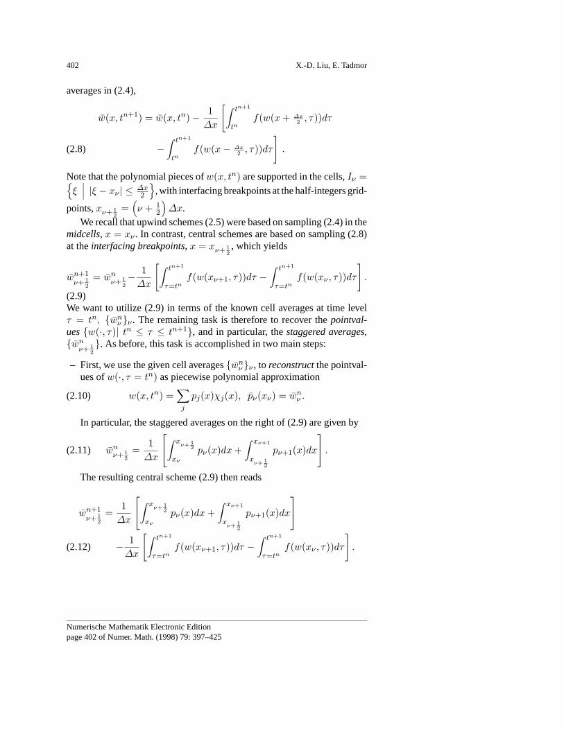
averages in (2.4),

w(x, tn+1) = w(x, tn) − 1∆x

[∫ tn+1

tnf(w(x + ∆x

2 , τ))dτ

−∫ tn+1

tnf(w(x − ∆x

2 , τ))dτ

].(2.8)

Note that the polynomial pieces ofw(x, tn) are supported in the cells,Iν ={ξ |ξ − xν | ≤ ∆x

2

}, with interfacing breakpoints at the half-integers grid-

points,xν+ 12

=(ν + 1

2

)∆x.

We recall that upwind schemes (2.5) were based on sampling (2.4) in themidcells, x = xν . In contrast, central schemes are based on sampling (2.8)at theinterfacing breakpoints, x = xν+ 1

2, which yields

wn+1ν+ 1

2= wn

ν+ 12− 1

∆x

[∫ tn+1

τ=tnf(w(xν+1, τ))dτ −

∫ tn+1

τ=tnf(w(xν , τ))dτ

].

(2.9)We want to utilize (2.9) in terms of the known cell averages at time levelτ = tn, {wn

ν }ν . The remaining task is therefore to recover thepointval-ues{w(·, τ)| tn ≤ τ ≤ tn+1}, and in particular, thestaggered averages,{wn

ν+ 12}. As before, this task is accomplished in two main steps:

– First, we use the given cell averages{wnν }ν , to reconstructthe pointval-

ues ofw(·, τ = tn) as piecewise polynomial approximation

w(x, tn) =∑j

pj(x)χj(x), pν(xν) = wnν .(2.10)

In particular, the staggered averages on the right of (2.9) are given by

wnν+ 1

2=

1∆x

∫ x

ν+12

xν

pν(x)dx +∫ xν+1

xν+1

2

pν+1(x)dx

.(2.11)

The resulting central scheme (2.9) then reads

wn+1ν+ 1

2=

1∆x

∫ x

ν+12

xν

pν(x)dx +∫ xν+1

xν+1

2

pν+1(x)dx

− 1∆x

[∫ tn+1


∫ tn+1


].(2.12)



Fig. 2.2. Central differencing by Godunov-type scheme

– Second, we follow theevolutionof the pointvalues along the mid-cells,x = xν , {w(xν , τ ≥ tn)}ν , which are governed by

wt + f(w)x = 0, τ ≥ tn; w(x, tn) = pν(x) x ∈ Iν .(2.13)

Let {ak(u)}k denote the eigenvalues of the JacobianA(u) := ∂f∂u . By

hyperbolicity, information regarding the interfacing discontinuities at(xν± 1

2, tn) propagates no faster thanmax

k|ak(u)|. Hence, the mid-cells

values governed by (2.13),{w(xν , τ ≥ tn)}ν , remain free of discon-tinuities, at least for sufficiently small time step dictated by the CFLcondition∆t ≤ 1

2∆x · maxk

|ak(u)|. Consequently, since the numerical

fluxes on the right of (2.12),∫ tn+1

τ=tn f(w(xν , τ))dτ , involve only smoothintegrands, they can be computed within any degree of desired accuracyby an appropriate quadrature rule.

It is the staggeredaveraging over the fan of left-going and right-goingwaves centered at the half-integered interfaces,(xν+ 1

2, tn), which charac-

terizes thecentral differencing, consult Fig. 2.2. A main feature of thesecentral schemes – in contrast to upwind ones, is the computation ofsmoothnumerical fluxes along the mid-cells,(x = xν , τ ≥ tn), which avoids thecostly (approximate) Riemann solvers. A couple of examples of centralGodunov-type schemes is in order.

The first-order Lax-Friedrichs (LxF) approximation is the forerunner forsuch central schemes – it is based on piecewise constant reconstruction,w(x, tn) = Σpj(x)χj(x) with pj(x) = wn

j . The resulting central scheme,(2.12), then reads (with the usual fixed mesh ratioλ := ∆t

∆x )

wn+1ν+ 1

2=

12(wν + wν+1) − λ

[f(wν+1) − f(wν)

].(2.14)

Nessyahu and Tadmor introduced in [NT] a second-order extension alongthese lines. Using the piecewise-linear MUSCL reconstruction,

w(x, tn) =∑

pj(x)χj(x), with pj(x) = wnj + w′

j

(x − xj

∆x

),



leads to a straightforward evaluation of staggered averages

wnν+ 1

2:=

1∆x

∫ xn+1

xj

w(x, tn)dx

=12(wn

ν + wnν+1) +

18(w′

ν − w′ν+1).(2.15)

The numerical flux is approximated by the second-order midpoint quadraturerule ∫ tn+1

τ=tnf(w(xν , τ))dτ ∼ ∆t · f(w(xν , t

n+ 12 )).

Here, the pointwise values at the half-time steps are evaluated by Tay-lor expansion (– recall the smoothness of (2.13) along the cell interfaces,(xν , τ ≥ tn)),

w(xν , tn+ 1

2 ) ∼ w(xν , t) +∆t

2wt(xν , t

n)

= wnν − ∆t

2A(wn

ν )(pν(xν , tn))x = wn

ν − λ

2An

νw′ν .

In summary, we end up with the central scheme, [NT], which consists of afirst-orderpredictor step,

wn+ 1

2ν = wn

ν − λ

2An

νw′ν , An

ν := A(wnν ),(2.16)

followed by the second-ordercorrector step, (2.12),

wn+1ν+ 1

2=

12(wn

ν + wnν+1) +

18(w′

ν − w′ν+1) − λ

[f(w

n+ 12

ν+1 ) − f(wn+ 1

2ν )

].

(2.17)

Thescalarnon-oscillatory properties of (2.16)–(2.17) were proved in [NT],[NTT], including TVD, cell entropy inequality,L1

loc− error estimates. . .Moreover, the numerical experiments, reported in [Ne], [NT], [ASV], [TW],with one- and multi-dimensionalsystemsof conservation laws, show thatsuch second-order central schemes enjoy the same high-resolution as the cor-responding second-order upwind schemes do. Thus, the excessive smearingtypical to the first-order LxF central scheme is compensated here by thesecond-order accurate MUSCL reconstruction.

At the same time, the central scheme (2.16)–(2.17) has the advantageover the corresponding upwind schemes, in that no (approximate) Riemannsolvers, as in (2.7), are required. Hence, these Riemann-free central schemesprovide an efficient high-resolution alternative in the one-dimensional case,and a particularly advantageous framework for multidimensional computa-tions, e.g., [AV], [ASV], [JT]. Also,staggeredcentral differencing, along the



lines of the Riemann-free Nessyahu-Tadmor scheme (2.16)–(2.17), admitssimple efficient extensions in the presence of general source terms, [Er], andin particular, stiff source terms, [BS]. Indeed, it is a key ingredient behindthe relaxation schemes studied in [JX], . . .

It should be noted, however, that the component-wise version of thesecentral schemes might result in deterioration of resolution at the computedextrema. Of course, this – so called extrema clipping, is typical to high-resolution upwind schemes as well; but it is more pronounced with ourcentral schemes due to the built-in extrema-switching to the dissipative LxFscheme. Indeed, once an extrema cell,Iν , is detected (by the limiter), it setsa zero slope,w′

ν = 0, in which case the second-order scheme (2.16)–(2.17)is reduced back to the first-order LxF, (2.14).

With this in mind, we now turn to discuss athird-orderaccurate Godunov-type central scheme along the above lines. It offers an improved resolutionover the second-order central scheme (2.16)–(2.17), and in particular, thisadditional accuracy compensates for the lost resolution at the clipped ex-trema.

3 Third-order central Godunov-type scheme

In this section we introduce our new third-order, non-oscillatory centralGodunov-type scheme. Following the framework outlined in Sect. 2, theconstruction of such scheme consists of two main ingredients:

(i) A third-order, piecewise-quadratic polynomial reconstruction which en-joys desirable non-oscillatory properties;

(ii) An appropriate quadrature rule to approximate the numerical fluxesalong cells’ interfaces.

We first address thescalar problem. And again, it should be remindedthat since our central scheme avoids (approximate) Riemann solvers, itsextension tosystemsmay proceed by a straightforwardcomponent-wiseap-plication of the scalar recipe – no characteristic decompositions are required.

3.1 Third-order non-oscillatory reconstruction

We shall use the third-order non-oscillatory reconstruction of Liu and Osher[LO]. Here is a reader’s digest for this reconstruction.

We start by seeking quadratic polynomials,qj(x) = aj + bj

(x−xj

∆x

)+

cj

(x−xj

∆x

)2, such that the piecewise parabolic reconstruction,w(x, tn) =

Σqj(x)χj(x), satisfies the two properties of:

P1 Conservation. Conserving the given cell-averages,{wnj }j



w(x, tn)|x=xj= wn

j(3.1)

P2 Accuracy. Third-order accuracy

w(x, tn) = u(x, tn) + O((∆x)3).(3.2)

To satisfyP1 andP2, one constructs a quadratic polynomial,qj(x), whosesliding averages interpolatewj (– that is, propertyP1), and, in addition, itinterpolates the two neighboring cell averages,wn

j±1. The three constrainsthen determine the unique parabola1

qj(x) =(

wnj − 1

24∆+∆−wn

j

)+ ∆0w

nj

(x − xj

∆x

)

+12∆+∆−wn

j ·(

x − xj

∆x

)2,(3.3)

which satisfies both (3.1) and (3.2). Moreover, since

q′j(xj− 1

2)q′

j(xj+ 12) = ∆−wj · ∆+wj/(∆x)2,

it follows that the quadratic reconstruction in (3.3) satisfies the importantproperty of

P3 Shape-preserving. qj(x) has the same shape as∑j+1

i=j−1 wni χi, that is,

– qj(x) is monotone (onIj) iff the cell averages{wnj−1, w

nj , wn

j+1} are;– qj(x) admits an extremum value in the interior ofIj iff wn

j is anextremum value (w.r.twn

j±1).

The shape preserving propertyP3 tells us that the piecewise-parabolic re-construction,w(x, tn) =

∑j qj(x)χj(x), creates no new extrema at the

interior of the cells,Ij ’s; thus, spurious extrema, if any, can be createdonlyat interfaces where

sgn(qj+1(xj+ 12) − qj(xj+ 1

2)) 6= sgn(wn

j+1 − wnj ).

To avoid such spurious extrema, we now turn to the last (– and essential) stepof limiting the reconstruction. To this end we consider convex modificationof the form

pj(x) = wnj + θj(qj(x) − wn

j ), 0 < θj < 1.(3.4)

Sincep′j(x) = θjq

′j(x), propertiesP1 andP3 remain valid. Moreover, a

limiter θj is sought so that(1 − θj) is proportional to the interface jump,qj+1(xj+ 1

2)− qj(xj+ 1

2); by the third-order accuracy ofq(·), the size of this

jump – and hence of(1−θj), is of orderO((∆x)3), and hence the modifiedquadratic,pj(x) remains third-order accurate ( – propertyP2). Finally, it

1 We denote, as usual,∆±w(x) = ±(w(x ± ∆x) − w(x)) and∆0 = 12 (∆+ + ∆−)



remains to specifyθj so as to eliminate spurious interface extrema. Oneconstructs such a limiterθj in terms of the cell quantities,

Mj = maxx∈Ij

qj(x), mj = minx∈Ij

qj(x),(3.5)

(one need not actually compute these extremal values as we shall clarify ina moment), and,

Mj± 1

2= max

{12(wn

j + wnj±1), qj±1(xj± 1

2)}

,

mj± 12

= min{

12(wn

j + wnj±1), qj±1(xj± 1

2)}

.(3.6)

The limiterθj is then given by

θj =

min{

Mj+1

2−wn

j

Mj−wnj

,m

j− 12

−wnj

mj−wnj

, 1}

, if wnj−1 < wn

j < wnj+1,

min{

Mj− 1

2−wn

j

Mj−wnj

,m

j+12

−wnj

mj−wnj

, 1}

, if wnj−1 > wn

j > wnj+1,

1 otherwise(if ∆+wn

j · ∆−wnj < 0).

(3.7)

Remark.We observe that the limiterθj is ‘switched-on’ only when the cellaverages,{wn

j−1, wnj , wn

j+1}, form a monotone sequence, which in turn,by the shape-preserving propertyP3, implies thatqj(x)|x∈Ij

is monotone.Hence, the pair of cell quantities{Mj , mj} in (3.5) admits one of the fol-lowing two explicit values: either{Mj , mj} = {qj(xj+ 1

2), qj(xj− 1

2)} in

the first increasing case, and in particular,Mj+ 12− Mj andmj− 1

2− mj are

of orderO((∆x)3); or, {Mj , mj} = {qj(xj− 12), qj(xj+ 1

2)} in the second

decreasing case, and in particular,Mj− 12−Mj andmj+ 1

2−mj are of order

O((∆x)3). Consequently, in both cases,θj in (3.7) is a third-order limiteras asserted, for1 − θj = O((∆x)3).

It was shown in [LO] that with this choice ofθj ’s, the resulting quadraticreconstruction satisfies

P4 Non-oscillatory property. The piecewise-quadratic reconstruction is non-oscillatory in the sense that

sgn(pj+1(xj+ 12) − pj(xj+ 1

2)) = sgn(wn

j+1 − wnj ).(3.8)

In summary, the resulting piecewise parabolic reconstruction,w(x, tn) =Σpj(x)χj(x), consists of quadratic pieces of the form

pj(x) = wnj + w′

j

(x − xj

∆x

)+

12w′′

j

(x − xj

∆x

)2.(3.9)



Here,w′′j are the (pointvalues of) thereconstructed second derivatives

w′′j := θj∆+∆−wn

j ;(3.10)

w′j are the (pointvalues of) thereconstructed slopes,

w′j := θj∆0w

nj ;(3.11)

andwnj are thereconstructed pointvalues

wnj := wn

j − w′′j

24.(3.12)

Observe that, starting with third- (and higher-) order accurate methods,pointwise valuescannotbe interchanged with cell averages,wn

j 6= wnj .

By propertiesP1 andP2, w(x1, tn) = Σpj(x)χj(x) is a third-order

cell conservative reconstruction. By propertiesP3 and P4, it is a non-oscillatory reconstruction in the sense thatN(w(·, tn)) – the number ofextrema ofw(x, tn), does not exceed that of its piecewise-constant projec-tion, N(Σwn

j χj(·)),N(w(·, tn)) ≤ N(Σwn

j χj(·)).(3.13)

We close this section by noting that one can further modify the limiterθj in (3.5)–(3.7), consult [LO], so that the resulting quadratic reconstruc-tion (3.9)–(3.12) satisfies – in addition to the NED property (3.13), alsothe strict maximum principleproperty,‖w(·, tn)‖L∞ ≤ ‖Σwn

j χj(·)‖L∞ .Consequently, the corresponding third-order reconstruction is total-variationnon-increasing.

3.2 The third-order scheme – scalar equations

The third-order accurate reconstruction of Sect. 3.1 is evolved in time usingthe central Godunov-type framework outlined in (2.9),

wn+1ν+ 1

2= wn

ν+ 12− 1

∆x

[∫ tn+1


∫ tn+1


].

(3.14)To this end we need to evaluate the staggered averages,{wn

ν+ 12}, and to

approximate the interface fluxes,{∫ tn+1

τ=tn f(w(xj , τ))dτ}

.

With pj(x) = wnj + w′

j

(x−xj

∆x

)+ 1

2w′′j

(x−xj

∆x

)2specified in (3.9)–

(3.12), one evaluates the staggered averages of the third order reconstruction



w(x, tn) = Σpj(x) χj(x)

wnν+ 1

2=

1∆x

∫ xν+1

xν

w(x, tn)dx =12(wν + wν+1) +

18(w′

ν − w′ν+1).

(3.15)

Remarkably, we obtain here the same formula for the staggered averages asin the second-order cases, consult (2.15); the only difference is the use ofthe new limited slopes in (3.11),w′

j = θj∆0wnj .

Next, we approximate the (exact) numerical fluxes by Simpson’s quadrat-ure rule, which is (more than) sufficient for retaining the overall third-orderaccuracy,

1∆x

∫ tn+1

τ=tnf(w(xν , τ))dτ ∼ λ

6

[f(wn

ν ) + 4f(wn+ 1

2ν ) + f(wn+1

ν )].

(3.16)

This in turn, requires the three approximatepointvalueson the right,wn+βν ∼

w(xν , tn+β) for β = 0, 1

2 , 1. Following our approach in the second-ordercase, [NT], we use Taylor expansion topredict

wnν ≡ w(xν , t

n) = wnν − w′′

ν

24,(3.17)

wn+ 1

2ν = wn

ν +λ

2wn

ν +λ2

8wn

ν ,(3.18)

wn+1ν = wn

ν + λwnν +

λ2

2wn

ν .(3.19)

Here, the first couple of time derivatives on the right are evaluated by exactdifferentiation of the quadratic reconstruction (3.9) (here and below,a(u)denotes the local speed,a(u) := fu(u)),

wnν = wn

ν − w′′ν

24;(3.20)

wnν ≡ (∆x · ∂t)w(xν , t

n) = −∆x · ∂xf(w(xν , tn))

= −a(wnν ) · w′

ν , ;(3.21)

wnν ≡ (∆x · ∂t)2w(xν , t

n)= ∆x · ∂x [a(wn

ν )∆x · ∂xf(w(xν , tn))](3.22)

= a2(wnν )w′′

ν + 2a(wnν )a′(wn

ν )(w′ν)

2.

These evaluations of Taylor expansions could be substituted by the moreeconomical Runge-Kutta integrations; the simplicity becomes more pro-nounced withsystemswhich is the next issue in our discussion.



In summary of the scalar setup, we end up with a two step scheme where,starting with the reconstructed pointvalues

wnν = wn

ν − w′′ν

24,(3.23)

we predictthe pointvalueswn+βν by, e.g. Taylor expansions,

wn+βν = wn

ν + λβwnν +

(λβ)2

2wn

ν , β =12, 1;(3.24)

this is followed by thecorrectorstep

wn+1ν+ 1

2=

12(wn

ν + wnν+1) +

18(w′

ν − w′ν+1)(3.25)

−λ

6

{[f(wn

ν+1) + 4f(wn+ 1

2ν+1 ) + f(wn+1

ν+1)]

−[f(wn

ν ) + 4f(wn+ 1

2ν ) + f(wn+1

ν )]}

.

3.3 The third-order scheme – systems

We use the ingredients of the scalar scheme in Sect. 3.2, to construct thethird-order approximation for systems of conservation laws. The attractivefeature is simplicity – these Riemann-free ingredients involve simple alge-braic manipulations which admits a straightforwardcomponent-wiseexten-sion to systems. By assembling the ingredients in Sect. 3.2 we arrive at thefollowing predictor-corrector scheme.

First, wepredict the pointvalues, wn+βν , β = 1

2 , 1,

wn+βν = wn

j − λβAnνw′

ν +(λβ)2

2

{(An

ν )2w′′ν + 2An

νBnν [w′

ν , w′ν ]}

.

(3.26)

Here, Anν ≡ A(wn

ν ) and Bnν = B(wn

ν ) are, respectively, the Jacobianof f(·), Aij = ∂fi

∂uj, and the corresponding 3-tensor,Bijk = ∂fi

∂uj∂uk, and

wnν , w′

ν , w′′ν are the vectors of pointvalues and their couple of derivatives,

derived from the non-oscillatory quadratic reconstruction in Sect. 3.1:

w′′ν = Θν(wn

ν+1 − 2wnν + wn

ν−1)

w′ν =

12Θν(wn

ν+1 − wnν−1)

wν = wnν − 1

24w′′

ν .

A couple of remarks is in order.



– The limiter. Here we include the possibility of amatrixlimiter,Θν , whichtakes into account Roe-like decompositions into characteristic waves[Ro]. As already noted in [NT], however, one of the main advantages ofour central-staggered framework over that of the upwind schemes, is thatsuch expensive and time-consuming characteristic decompositions canbe avoided. Specifically, all the non-oscillatory computations reportedin Sect. 5 below were carried out with diagonal limiters,Θν , based on acomponent-wiseextension of the scalar limiters outlined in (3.5)–(3.7).

– Taylor vs. Runge-Kutta expansion. There is a variety of more economicalalternatives to Taylor expansion used for the predictor step in (3.26). Forexample, the explicit evaluation of the 3-tensorBn

ν on the right of (3.26)can be avoided if the exact spatial derivatives inside the curly bracketson the right of (3.26),(A2wx)x, are replaced by an approximate discreteone,{·}′

ν := Θν∆0{·}ν ,

wn+βν = wn

ν − λβAnνw′

ν +(λβ)2

2{(An

ν )2w′ν}′.(3.26′)

Still another alternative which utilizes the discrete derivative, is thesecond-order Runge-Kutta, which reads

wn+βν = wn

ν − λβ

{f

(wn

ν − λβ

2An

νw′ν

)}′.(3.26′′)

And an even more greedy version is the second-order Runge-Kuttawhich does not require the computation of any Jacobian,

wn+βν = wn

ν − λβ

{f

(wn

ν − λβ

2{f(wn

ν )}′)}′

.(3.26′′′)

The numerical experiments reported in this paper utilize the predictorstep in its basic version (3.26). As expected, its exactly differentiated termsseem to provide a slightly more accurate results than the more econom-ical versions in (3.26′)–(3.26′′′). We should point out, however, that thelatter, Jacobian-free versions (3.26′-3.26′′′), are still offering economical al-ternatives – our numerical experiments, e.g., [TW], show that they retainessentially the same high-resolution as the basic version (3.26).

Equipped with the predicted pointvalues in (3.26), together with Simp-

son’s quadrature (3.16), we evaluate the approximate flux,fn+ 1

2ν ,

fn+ 1

2ν :=

16

[(f(wn

ν ) + f(wn+ 1

2ν ) + f(wn+1

ν )];(3.27′)



these approximate fluxed are then used with the exact staggered averaging,(3.15), in order to evaluate the cell averages of the next time level,t = tn+1,by the central recipe (3.14),

wn+1ν+ 1

2=

12(wn

ν + wnν+1) +

18(w′

ν − w′ν+1) − λ

[f

n+ 12

ν+1 − fn+ 1

2ν

],

(3.27′′)

The predictor-corrector scheme (3.26)–(3.27′′), expressed in terms of thepointwise limited derivatives,wn

ν , w′ν and w′′

ν , form our third-order non-oscillatory central scheme.

4 Stability of the scalar scheme (the NED property)

In this section we make a precise assertion regarding the non-oscillatorybehavior of our third-order central scheme in the scalar case.

Our starting point is theexactstaggered averaging of the scalar piece-wise-quadratic reconstruction,

w(x, tn) =∑j

[wn

j + w′j

(x − xj

∆x

)+

12w′′

j

(x − xj

∆x

)2]

χj ,

which yields the corrector scheme (3.14)–(3.15)

wn+1ν+ 1

2=

12(wν + wν+1) +

18(w′

ν − w′ν+1)

− 1∆x

[∫ tn+1

τ=tnf(wν+1(τ))dτ −

∫ tn+1

τ=tnf(wν(τ))dτ

].(4.1)

Here,wν(τ) = w(xν , τ ≥ tn) are the mid-cells pointvalues governed by,consult (2.13)

wt + f(w)x = 0, τ ≥ tn,(4.2)

w(x, τ = tn) = wnν + w′

ν

(x − xν

∆x

)+

12w′′

ν

(x − xν

∆x

)2,(4.3)

x ∈ Iν .

To approximatethe temporal integrals on the right of (4.1), Simpson’squadrature rule, (3.16), followed by Taylor expansions, (3.17)–(3.19), wereused. We note that, at least in the scalar case under consideration, one canevaluate these integralsexactlyin a straightforward manner. Indeed, thanksto the central staggering, the mid-cells(xν , τ ≥ tn) are ‘secured’ insidea smooth region where the local speedaν = a(wν(τ)) satisfies a simple



quadratic(aν = a(wν−saνw′ν+ 1

2(saν)2w′′ν)), whose approximate solution

yields

a(wν(τ)) =a(wn

ν )1 + sa′(wn

ν )w′ν

[1 +

a(wnν ) · s2w′′

ν

2(1 + sa′(wnν )w′

ν)2+ O(s4)

],

s :=τ − tn

∆x.

Our first main result asserts the non-oscillatory behavior of the centralscheme (4.1) based on the above mentionedexactflux evaluation.

Proposition 1 Consider the central scheme (4.1)–(4.3), based on the third-order accurate quadratic reconstruction, (3.9)–(3.12). Then it satisfies theso-called Number of Extrema Diminishing (NED) property, in the sense that

N

(∑ν

wn+1v+ 1

2χν+ 1

2(x)

)≤ N

(∑ν

wnν χν(x)

).(4.4)

Proof We first recall that the quadratic reconstruction,w(·, tn), in (3.9)–(3.12) is non-oscillatory in the sense of satisfying the NED property, consult(3.13),

N(w(·, tn)) ≤ N

(∑ν

wnν χν(·)

).

Next we consider thesliding averageof the reconstruction,w(x, tn) =1

∆x

∫Ix

w(ξ, tn)dξ; clearly, sincew(·, t) = w(·, tn)∗ 1∆xχ0, with the positive

mollifier 1∆xχ0, we have

N(w(·, tn)) ≤ N(w(·, tn)).

Finally, we study the governing equation forw(·, t): by averaging (4.2)we find an averages-pointvalues relation similar to (2.2), which we rewriteas

wt(x, t) + a(x, t)wx(x, t) = 0.(4.5)

Here,a denotes the averaged speed,a :=∫ 1η=0 a[w(x− ∆x

2 , t)+ η∆w(x−∆x2 , t)]dη.

Thus, the sliding average,w(·, t), is aC1-solution of thetransport equation(4.5), and as such it satisfies

N(w(·, tn+1)) ≤ N(w(·, tn)).

In particular, by sampling at the mid-cells(xν+ 12, tn+1), we have

N

(∑ν

wn+1ν+ 1

2χν+ 1

2(x)

)≤ N(w(·, tn+1)) .

This, together with the previous last three inequalities yields the NED prop-erty (4.4). ut



Remarks.

1. Harten and Osher proved the NED property for theiruniformlysecond-order non-oscillatory scheme [HO]. In particular, the NED property en-ables to circumvent the limitation of first-order clipping phenomena inTVD schemes [OT]. (Observe that the limiterθj in (3.7) isnot‘switched-on’ at extrema whereθj = 1. If instead, we setθj = 0 in those cases,we run into the familiar ’clipping’ phenomena, where we avoid increas-ing extrema, at the expense of reducing to the first-order accurate LxFscheme).

2. Let TV (w(·, tn)) =∑

ν |wnν+1 − wn

ν | denote the total-variation of thepiecewise-constant approximation oft = tn, then the following straight-forward upper-trend holds

TV (w(·, tn)) ≤ 2N

(∑ν

wnν χν(·)

)‖∑

wnν χν(·)‖L∞ .

Thus, the NED property together with an additionalL∞-bound implyTotal Variation boundednessTV (w(·, tn)) ≤ Const., and hence the con-vergence of the approximate solutions.

3. As we have already noted before, one can modify the limiter in (3.5)–(3.7), consult [LO], so that the resulting quadratic reconstruction (3.9)–(3.12) satisfies a (strict) maximum principle, in addition to the NEDproperty. Consequently, the corresponding third-order central scheme(4.1)–(4.3) based on such modified limiter, is total-variation bounded andhence convergent. We found, however, that the enforcement of an addi-tional (strict) maximum principle is neither necessary (in the scalar case),nor is it recommended for systems (which need not satisfy acomponent-wisemaximum principle). Finally, our numerical experiments also showthat the conclusion of Proposition 1 remains valid with Simpson’s rule(3.16) replacing the exact flux evaluations on the right of (4.1).

5 Numerical experiments

5.1 Scalar conservation laws

In this section we use some model problems to numerically test our schemes,(3.23)–(3.25). In the scalar context, we used the modified nonoscillatorylimiter, which enforces the (strict) maximum principle, [LO].

Example 1 (Transport equation). We solve the model transport equation

ut + ux = 0, −1 ≤ x ≤ 1,(5.1)

subject to2-periodic initial data,u(x, 0) = u0(x).



Table 5.1. Linear transport equation (5.1) withu0 = sin(πx). Errors att = 10. (mesh-ratioλ = 0.45)

N L1 error L1 order L∞ error L∞ order20 5.98608D−03 4.65946D−0340 7.22214D−04 3.05 5.65980D−04 3.0480 8.83936D−05 3.03 6.93894D−05 3.03

Table 5.2. Linear transport equation (5.1) withu0 = sin4(πx). Errors att = 1. (mesh-ratioλ = 0.45)


Two sets of initial datau0(x) were used: the first one isu0(x) = sin(πx);Table 5.1 quotes theL1 andL∞ errors att = 10. The second one isu0(x) =sin4(πx), and we list the errors, recorded at timet = 1. in Table 5.2.

Remark.Here, and in all the examples below,N denotes the total numberof spatial cells, and∆x is the gridsize given by∆x = 2

N . Lp errors aremeasured by the difference between the pointvalues of the “exact” solu-tion, u(xν , t

n), and thereconstructedpointvalues of the computed solution(consult (3.12)),wn

ν = wnν − 1

24w′′ν .

For these two sets of initial data, we obtain third-order of accuracy inthe smooth region in bothL1 andL∞ norms. We note that standard ENOapproximations of (5.1) with the second set of initial data, experiences an(easily fixed) loss of accuracy, see [RM], [Sh]. No such degeneracy wasfound with our present method. Indeed, as noted by Shu, [Sh], the class ofcentered schemes are particularly good candidates – in terms of uniformconvergence, independently of the initial data.

Example 2 (Propagation of singularities).Here we consider the transportequation (5.1) initialized with the 2-periodicdiscontinuouscharacteristicfunction,u0(x) = χ0 = 1− 1

2≤x≤ 12. We observe the good resolution of the

computed solution in Fig. 5.1. As expected, the viscous profile spreads overa transition layer of sizes(∆x)

34 , sharpening the first- and second-order

shock layers of the corresponding size√

∆x and(∆x)23 . This sharpening

will be borne out in our later numerical experiments, with the improvedresolution of contact discontinuities in the system of Euler’s equations.

Example 3 (Nonlinear transport equation).We solve the canonical, inviscidBurgers’ equation

ut + (12u2)x = 0, −1 ≤ x ≤ 1,(5.2)



-1 -0.8 -0.6 -0.4 -0.2 0 0.2 0.4 0.6 0.8 10

0.1

0.2

0.3

0.4

0.5

0.6

0.7

0.8

0.9

1The third-order solution at T = 2

-- true solu ++ approx. solu N=80

dt/d

x =

0.3

3

Fig. 5.1. Linear transport equation (5.1) withu0 = 1− 12 ≤x≤ 1

2computed att = 2. (mesh-

ratioλ = 0.45)

Table 5.3. Inviscid Burgers’ equation (5.2) withu0(x) = 1 + 12sin(πx). Errors att = 0.3

(mesh-ratioλ = 0.33)

N L1 error L1 order L∞ error L∞ order80 4.28013−05 1.13262D−04160 5.82855−06 2.87 2.35429D−05 2.27320 9.04921−07 2.69 4.91819D−06 2.26640 1.59062−07 2.51 1.03645D−06 2.451280 2.7007D−08 2.55 2.16767D−07 2.26

subject to 2-periodic initial datau0(x) = 1 + 12sin(πx).

Recall that the exact solution is smooth up to the critical timet = 2π ∼

0.6366. In Table 5.3 we list the errors att = 0.3. Note that we have close tothird-order accuracy inL1, and more than second-order of accuracy inL∞.

At t = 2π , the Burgers’ equation develops a moving shock which then

interacts with a rarefaction wave; att = 1.1 the interaction between theshock and the rarefaction waves is over, and the solution becomes monotonebetween shocks. In Figs. (5.2)–(5.3) we observe the excellent agreementbetween the exact and the non-oscillatory computed solution, in both stagesof the developed discontinuity. In particular, Table 5.4 records theL1 andL∞errors in the smooth portion of the solution, bounded away from the movingdiscontinuity. Third-order accuracy in both inL1 andL∞ is observed in thesmooth portion – at distance0.1 away from the shock. The errors are ofsmaller magnitude than the ones in the smooth case, showing the reductionin error propagation.



-1 -0.8 -0.6 -0.4 -0.2 0 0.2 0.4 0.6 0.8 10.5

0.6

0.7

0.8

0.9

1

1.1

1.2

1.3

1.4

1.5The third-order solution at T = 0.6366


dt/d

x =

0.3

3

Fig. 5.2. Burgers’ equation (5.2) withu0(x) = 1 + 12sin(πx) computed att = 0.6366

-1 -0.8 -0.6 -0.4 -0.2 0 0.2 0.4 0.6 0.8 10.5

0.6

0.7

0.8

0.9

1

1.1

1.2

1.3

1.4

1.5The third-order solution at T = 1.1


dt/d

x =

0.3

3

−1 −0.8 −0.6 −0.4 −0.2 0 0.2 0.4 0.6 0.8 10.4

0.6

0.8

1

1.2

1.4

1.6The third−order solution at T = 1.1

−− true solu ++ approx. solu N=80

dt/h

= 0

.3

Fig. 5.3. Burgers’ equation (5.2) withu0(x) = 1 + 12sin(πx) computed att = 1.1.

Nonoscillatory limiter: with enforcement of maximum principle (– on left) and without (–on right)

Finally, we note that in Fig. (5.3) we record the results based on thetwo versions of the nonoscillatory limiter (3.5)–(3.7): the figure on the leftutilizes themodifiedversion which enforces the additional the maximumprinciple, [LO], and it is compared with the figure on the right, where thebasic version of the NED limiter is used without the enforcement of an extramaximum principle. It is evident that we retain the same quality resultsin both cases. This promotes us to concentrate, in the case of systems, onthe nonoscillatory limiter in its basic version, (3.5)–(3.7), without the extraenforcement of the maximum principle.



0 0.1 0.2 0.3 0.4 0.5 0.6 0.7 0.8 0.9 10.1

0.2

0.3

0.4

0.5

0.6

0.7

0.8

0.9

1

Sod’s problem by third-order central scheme with N=200 points

DE

NS

ITY

at

T=

0.1

64

4 (

dt/

dx

=0

.1)

0.0 0.2 0.4 0.6 0.8 1.0Sod’s problem by 2nd-order STG scheme with N=200 points

0.0

0.2

0.4

0.6

0.8

1.0

DEN

SITY

0 0.1 0.2 0.3 0.4 0.5 0.6 0.7 0.8 0.9 10

0.1

0.2

0.3

0.4

0.5

0.6

0.7

0.8

0.9

1


VE

LO

CIT

Y a

t T

=0

.16

44

(d

t/d

x=

0.1

)


0.0

0.2

0.4

0.6

0.8

1.0

VELO

CIT

Y

0 0.1 0.2 0.3 0.4 0.5 0.6 0.7 0.8 0.9 10.1

0.2

0.3

0.4

0.5

0.6

0.7

0.8

0.9

1


PR

ES

SU

RE

at

T=

0.1

64

4 (

dt/

dx

=0

.1)


0.0

0.2

0.4

0.6

0.8

1.0

PRES

SUR

E

Fig. 5.4. Third- vs. second-order central schemes – Riemann problem with Sod’s initial data(5.4) computed att = 0.1644



0 0.1 0.2 0.3 0.4 0.5 0.6 0.7 0.8 0.9 10.2

0.4

0.6

0.8

1

1.2

1.4

Lax’s problem by third-order central scheme with N=200 points

DE

NS

ITY

at

T=

0.1

6 (

dt/

dx

=0

.1)

0.0 0.2 0.4 0.6 0.8 1.0Lax’s problem by second-order upwind scheme with N=200 points

0.0

0.2

0.4

0.6

0.8

1.0

1.2

1.4

DEN

SITY

0 0.1 0.2 0.3 0.4 0.5 0.6 0.7 0.8 0.9 10

0.2

0.4

0.6

0.8

1

1.2

1.4

1.6


VE

LO

CIT

Y a

t T

=0

.16

(d

t/d

x=

0.1

)


0.0

0.5

1.0

1.5

2.0

VELO

CIT

Y

0 0.1 0.2 0.3 0.4 0.5 0.6 0.7 0.8 0.9 10.5

1

1.5

2

2.5

3

3.5

4


PR

ES

SU

RE

at

T=

0.1

6 (

dt/

dx

=0

.1)


0.0

1.0

2.0

3.0

4.0

PRES

SUR

E

Fig. 5.5. Third-order central vs. second-order upwind schemes – Riemann problem withLax’s initial data (5.5) computed att = 0.16



0 0.1 0.2 0.3 0.4 0.5 0.6 0.7 0.8 0.9 10

1

2

3

4

5

6

7

W-C problem by third-order central scheme with N=400 points

DE

NS

ITY

at

T=

0.0

1 (

dt/

dx

= 0

.01

)

0.0 0.2 0.4 0.6 0.8 1.0W-C problem by second-order central scheme with N=400 points

0.0

1.0

2.0

3.0

4.0

5.0

6.0

DEN

SITY

AT

T=

0.01

0 0.1 0.2 0.3 0.4 0.5 0.6 0.7 0.8 0.9 1-10

-5

0

5

10

15

20


VE

LO

CIT

Y a

t T

=0

.00

1 (

dt/

dx

= 0

.01

)


-10.0

-5.0

0.0

5.0

10.0

15.0

20.0

VELO

CIT

Y A

T T

=0.0

1

0 0.1 0.2 0.3 0.4 0.5 0.6 0.7 0.8 0.9 10

50

100

150

200

250

300

350

400

450

500


PR

ES

SU

RE

at

T=

0.0

1 (

dt/

dx

= 0

.01

)


0.0

100.0

200.0

300.0

400.0

500.0

PRES

SUR

E A

T T

=0.0

1

Fig. 5.6. Third- vs. second-order central schemes – Woodward-Colella double blast waveswith initial data (5.7), computed att = 0.01



0 0.1 0.2 0.3 0.4 0.5 0.6 0.7 0.8 0.9 10

2

4

6

8

10

12

14

16

18

20


DE

NS

ITY

at

T=

0.0

3 (

dt/

dx

= 0

.01

)

0 0.1 0.2 0.3 0.4 0.5 0.6 0.7 0.8 0.9 10

1

2

3

4

5

6


DE

NS

ITY

at

T=

0.0

38

(d

t/d

x =

0.0

1)

0 0.1 0.2 0.3 0.4 0.5 0.6 0.7 0.8 0.9 1-10

-5

0

5

10

15


VE

LO

CIT

Y a

t T

=0

.03

(d

t/d

x =

0.0

1)

0 0.1 0.2 0.3 0.4 0.5 0.6 0.7 0.8 0.9 1-2

0

2

4

6

8

10

12

14

16


VE

LO

CIT

Y a

t T

=0

.03

8 (

dt/

dx

= 0

.01

)

0 0.1 0.2 0.3 0.4 0.5 0.6 0.7 0.8 0.9 10

100

200

300

400

500

600

700

800


PR

ES

SU

RE

at

T=

0.0

3 (

dt/

dx

= 0

.01

)

0 0.1 0.2 0.3 0.4 0.5 0.6 0.7 0.8 0.9 10

50

100

150

200

250

300

350

400


PR

ES

SU

RE

at

T=

0.0

38

(d

t/d

x =

0.0

1)

Fig. 5.7. Third-order central scheme – Woodward-Colella double blast waves with initialdata (5.7), computed att = 0.03 andt = 0.038



Table 5.4. Burgers’ equation (5.2) withu0(x) = 1 + 12sin(πx). L1, L∞ errors0.1 away

from the shock, i.e.|x − shock location| ≥ 0.1, att = 1.1 (mesh-ratioλ = 0.33)


5.2 Euler equations of gas dynamics

In this subsection we apply our third-order scheme to the Euler equationsof polytropic gas,

ut + f(u)x = 0,(5.3)

whereu = (ρ, m, E)T is the unknown vector of densityρ, momentum,m := ρq, and energyE, andf(u) is the corresponding flux,f(u) = qu +(0, p, qp)T expressed in terms of the pressure,p := (γ −1)(E − 1

2ρq2) witha fixedγ = 1.4.

Example 4 (Riemann problems).We consider the Riemann problems subjectto Riemann initial data,

u0(x) ={

ul x < 0ur x > 0.

Two sets of Riemann initial data are used: the one proposed by Sod in [So],

(ρl, ml, El) = (1, 0, 2.5), (ρr, mr, Er) = (0.125, 0, 0.25);(5.4)

and the one used by Lax [La]:

(ρl, ml, El) = (0.445, 0.311, 8.928),(ρr, mr, Er) = (0.5, 0, 1.4275).(5.5)

Figure 5.4 shows the third-order central results for Sod’s problem, incomparison to the corresponding second-order central results. Two majorimpovements should be pointed out:{i} A narrow transion layer with a considerably sharper resolution of thecontact wave (– an improvement already anticipated in the linear Example2 above);{ii}Third-order resolution improvement of the second-order results (– whichis most evident at the rarefaction tips).

Fig. 5.5 compares the results of the third-order central scheme with thesecond-order upwind ULT scheme of Harten [Ha]. In this context (of dif-ferent order of accuracy), we would like to emphasize the following twopoints:



{i} The sharper contact resolution by the third-order scheme;{ii} The improved resolution, particularly near the rarefaction tips; verymild oscillations, however, are detected in the third-order computation of thevelocity field. These are at the acceptable the level, once we take into accountthe simplicity and efficiency offered by ourcomponentwisecomputation vs.the complexity of the upwind characteristic approach.

Example 5 (Double blast waves).Our last example taken from Woodwardand Colella, [WC], describes the interaction of blast waves subject to initialconditions

u0(x) =

ul 0 ≤ x < 0.1,um 0.1 ≤ x < 0.9,ur 0.9 ≤ x < 1,

(5.6)

with

(ρl, ml, El) = (1, 0, 1000),(ρm, mm, Em) = (1, 0, 0.01),(ρr, mr, Er) = (1, 0, 100).

(5.7)

A solid wall boundary conditions (reflection) is applied to both ends. InFig. 5.6 we compare the third-order numerical results att = 0.01, with thecorresponding second-order computations of [NT]. Here we would like tohighlight:{i} Sharper resolution of the shock waves;{ii} Elimination of the extrema clipping which was evident in the second-order computation of the density in Fig. 5.6: observe that the density spike(on the right) has now the correct amplitude of∼ 5.2, up from the second-order ’clipped’ value of∼ 3.7.The numerical results computed at the later time,t = 0.03 andt = 0.038,are presented in Fig. 5.7. It is remarkable that the third-order central schemeis able to obtain such sharp resolution of the complex double blast problem,withoutany use of characteristic information, additional artificial compres-sion, ad hoc switches,etc.

Acknowledgements.Research was supported by Department of Energy Grant #DE.FG02-88ER25053 (X.-D. L), and by ONR Grant #N0014-91-J1076 and NSF Grant #DMS91-03104(E.T).

References

[ASV] Arminjon, P., Stanescu, D., Viallon, M.C. (1995):A two-dimensional finite volumeextension of the Lax-Friedrichs and Nessyahu-Tadmor schemes for compressibleflows. Proc.6th Intl. Symp. on Comp. Fluid Dynamics (M. Hafez, K. Oshima eds.),Lake Tahoe



[AV] Arminjon, P., Viallon, M.C. (1995): Generalisation du schema de Nessyahu-Tadmorpour uneequation. hyperboliquea deux dimensions d’espace. C.R. Acad. Sci. Paris,t. 320, serie I, pp. 85–88

[BS] Bereux, F., Sainsaulieu, L. (1997): A Roe-type Riemann solver for hyperbolicsystems with relaxation based on time-dependent wave decomposition. Numer.Math.77, 143–185

[CW] Colella, P., Woodward, P. (1984): The piecewise parabolic method (PPM) for gas-dynamical simulations. JCP54, 174–201

[Er] Erbes, G.: A high-resolution Lax-Friedrichs scheme for Hyperbolic conservationlaws with source term. Application to the Shallow Water equations. Preprint.

[Go] Godunov, S.K. (1959): A finite difference method for the numerical computation ofdiscontinuous solutions of the equations of fluid dynamics. Mat. Sb.47, 271–290

[Ha] Harten, A. (1983): High resolution schemes for hyperbolic conservation laws. JCP49, 357–393

[HEOC] Harten, A., Engquist, B., Osher, S., Chakravarthy, S.R. (1982): Uniformly highorder accurate essentially non-oscillatory schemes. III, JCP71, 231–303

[HO] Harten A., Osher, S. (1982): Uniformly high order accurate non-oscillatory scheme.I, SINUM 24, 229–309

[Hu] Huynh, H. (1995): A piecewise-parabolic dual-mesh method for the Euler equa-tions. AIAA-95-1739-CP, The 12th AIAA CFD Conf.

[JT] Jiang, G.S., Tadmor, E.: Non-oscillatory central schemes for multidimensional hy-perbolic conservation laws. SIAM J. Sci. Comput. (in press)

[JX] Jin, S., Xin, Z. (1995): The relaxation schemes for systems of conservation laws inarbitrary space dimensions. CPAM48, 235–276

[La] Lax, P.D. (1954): Weak solutions of non-nonlinear hyperbolic equations and theirnumerical computations. CPAM7, 159–193

[Le] van Leer, B. (1979): Towards the ultimate conservative difference scheme, V. Asecond order sequel to Godunov’s method. JCP32, 101–136

[LL] Liu, X.-D., Lax, P.D. (1996): Positive Schemes for Solving Multi-dimensionalHyperbolic Systems of Conservation Laws. CFD Journal5, 1–24

[LO] Liu, X.-D., Osher, S. (1996): Nonoscillatory high order accurate self similar max-imum principle satisfying shock capturing schemes. I. SINUM33, 760–779

[Ne] Nessyahu, N. (1987): Non-oscillatory second order central type schemes for sys-tems of nonlinear hyperbolic conservation laws. M.Sc. Thesis, Tel-Aviv University

[NT] Nessyahu, N., Tadmor, E. (1990): Non-oscillatory central differencing for hyper-bolic conservation laws. JCP87, 408–448

[NTT] Nessyahu, H., Tadmor, E., Tassa, T. (1994): On the convergence rate of Godunov-type schemes. SINUM31, 1–16

[OT] Osher, S., Tadmor, E. (1988): On the convergence of difference approximating toscalar conservation laws. Math. Comp.50, 15–51

[Ro] Roe, P. (1981): Approximate Riemann solvers, parameter vectors, and differenceschemes. JCP43, 357–372

[RM] Rogerson, A., Meiburg, E. (1990): A numerical study of the convergence propertiesof ENO schemes. J. Sci. Comput.5, 127–149

[Sa1] Sanders, R. (1988): A third-order accurate variation nonexpansive differencescheme for single conservation laws. Math. Comp.51, 535–558

[Sa2] Sanders, R.: Private communication[SW] Sanders, R., Weiser, A. (1992): A high resolution staggered mesh approach for

nonlinear hyperbolic systems of conservation laws. JCP1010, 314–329[Sw] Sweby, P. (1984): High resolution schemes using flux limiters for Hyperbolic con-

servation laws. SINUM21, 995–1001



[Sh] Shu, C.-W. (1990): Numerical experiments on the accuracy of ENO and modifiedENO schemes. JCP5, 127–149

[So] Sod, G. (1978): A survey of several finite difference methods for systems of non-linear hyperbolic conservation laws. JCP22, 1–31

[TW] Tadmor, E., Wu, C.C.: Central scheme for the multidimensional MHD equations.In preparation.

[WC] Woodward, P., Colella, P. (1988): The numerical simulation of two-dimensionalfluid flow with strong shocks. JCP54, 115–173


numerische mathematik - cscamm · numer. math. (1998) 79: 397–425 numerische mathematik c...

Documents