numpy tutorial - python · 2.14 c and fortran order ... the memory block •only changes the dtype...

Numpy tutorialRelease 2011

Pauli Virtanen

September 13, 2011

CONTENTS

1 Advanced Numpy 31.1 The Plan . . . . . . . . . . . . . . . . . . . . . . . . . . . . . . . . . . . . . . . . . . . . . . . . . 3

2 Numpy under the hood 52.1 It’s... . . . . . . . . . . . . . . . . . . . . . . . . . . . . . . . . . . . . . . . . . . . . . . . . . . . 52.2 Block of memory . . . . . . . . . . . . . . . . . . . . . . . . . . . . . . . . . . . . . . . . . . . . . 52.3 Sharing memory . . . . . . . . . . . . . . . . . . . . . . . . . . . . . . . . . . . . . . . . . . . . . 62.4 Flags . . . . . . . . . . . . . . . . . . . . . . . . . . . . . . . . . . . . . . . . . . . . . . . . . . . 62.5 Data types . . . . . . . . . . . . . . . . . . . . . . . . . . . . . . . . . . . . . . . . . . . . . . . . 72.6 Aside: casting . . . . . . . . . . . . . . . . . . . . . . . . . . . . . . . . . . . . . . . . . . . . . . 72.7 Data re-interpretation . . . . . . . . . . . . . . . . . . . . . . . . . . . . . . . . . . . . . . . . . . . 82.8 Data re-interpretation . . . . . . . . . . . . . . . . . . . . . . . . . . . . . . . . . . . . . . . . . . . 82.9 Not so fast! . . . . . . . . . . . . . . . . . . . . . . . . . . . . . . . . . . . . . . . . . . . . . . . . 92.10 Not so fast! . . . . . . . . . . . . . . . . . . . . . . . . . . . . . . . . . . . . . . . . . . . . . . . . 92.11 Indexing? . . . . . . . . . . . . . . . . . . . . . . . . . . . . . . . . . . . . . . . . . . . . . . . . . 92.12 Indexing: strides . . . . . . . . . . . . . . . . . . . . . . . . . . . . . . . . . . . . . . . . . . . . . 102.13 Indexing: strides (2) . . . . . . . . . . . . . . . . . . . . . . . . . . . . . . . . . . . . . . . . . . . 102.14 C and Fortran order? . . . . . . . . . . . . . . . . . . . . . . . . . . . . . . . . . . . . . . . . . . . 102.15 Indexing: Slicing . . . . . . . . . . . . . . . . . . . . . . . . . . . . . . . . . . . . . . . . . . . . . 112.16 Manual stride manipulation . . . . . . . . . . . . . . . . . . . . . . . . . . . . . . . . . . . . . . . 112.17 More strides: diagonals . . . . . . . . . . . . . . . . . . . . . . . . . . . . . . . . . . . . . . . . . 122.18 More strides: A small mistake... . . . . . . . . . . . . . . . . . . . . . . . . . . . . . . . . . . . . . 122.19 Summary of internals . . . . . . . . . . . . . . . . . . . . . . . . . . . . . . . . . . . . . . . . . . 12

3 Everyday features: Broadcasting 133.1 Scalars . . . . . . . . . . . . . . . . . . . . . . . . . . . . . . . . . . . . . . . . . . . . . . . . . . 133.2 Arrays? . . . . . . . . . . . . . . . . . . . . . . . . . . . . . . . . . . . . . . . . . . . . . . . . . . 133.3 Shape matching . . . . . . . . . . . . . . . . . . . . . . . . . . . . . . . . . . . . . . . . . . . . . 143.4 Higher dimensions: more of the same . . . . . . . . . . . . . . . . . . . . . . . . . . . . . . . . . . 143.5 Common uses (1/3) . . . . . . . . . . . . . . . . . . . . . . . . . . . . . . . . . . . . . . . . . . . . 153.6 Common uses (2/3) . . . . . . . . . . . . . . . . . . . . . . . . . . . . . . . . . . . . . . . . . . . . 153.7 Common uses (3/3) . . . . . . . . . . . . . . . . . . . . . . . . . . . . . . . . . . . . . . . . . . . . 153.8 Explicit broadcasting . . . . . . . . . . . . . . . . . . . . . . . . . . . . . . . . . . . . . . . . . . . 163.9 Ghost arrays . . . . . . . . . . . . . . . . . . . . . . . . . . . . . . . . . . . . . . . . . . . . . . . 16

4 Everyday features: Fancy indexing 194.1 Boolean masks . . . . . . . . . . . . . . . . . . . . . . . . . . . . . . . . . . . . . . . . . . . . . . 194.2 Boolean masks, ndim > 1 . . . . . . . . . . . . . . . . . . . . . . . . . . . . . . . . . . . . . . . . 194.3 Boolean masks, ndim > 1 . . . . . . . . . . . . . . . . . . . . . . . . . . . . . . . . . . . . . . . . 20

i

4.4 Integer indexing . . . . . . . . . . . . . . . . . . . . . . . . . . . . . . . . . . . . . . . . . . . . . 204.5 Integer indexing, simple . . . . . . . . . . . . . . . . . . . . . . . . . . . . . . . . . . . . . . . . . 214.6 Integer indexing + slices . . . . . . . . . . . . . . . . . . . . . . . . . . . . . . . . . . . . . . . . . 214.7 Integer indexing + slices . . . . . . . . . . . . . . . . . . . . . . . . . . . . . . . . . . . . . . . . . 214.8 Windows to data . . . . . . . . . . . . . . . . . . . . . . . . . . . . . . . . . . . . . . . . . . . . . 22

5 Everyday features: Structured data types 255.1 Composite data . . . . . . . . . . . . . . . . . . . . . . . . . . . . . . . . . . . . . . . . . . . . . . 255.2 Structured type . . . . . . . . . . . . . . . . . . . . . . . . . . . . . . . . . . . . . . . . . . . . . . 255.3 Loading from a text file . . . . . . . . . . . . . . . . . . . . . . . . . . . . . . . . . . . . . . . . . 265.4 Accessing fields . . . . . . . . . . . . . . . . . . . . . . . . . . . . . . . . . . . . . . . . . . . . . 265.5 Indexing &c. . . . . . . . . . . . . . . . . . . . . . . . . . . . . . . . . . . . . . . . . . . . . . . . 265.6 Some utility functions . . . . . . . . . . . . . . . . . . . . . . . . . . . . . . . . . . . . . . . . . . 275.7 Re-interpreting data as structured arrays . . . . . . . . . . . . . . . . . . . . . . . . . . . . . . . . . 275.8 Re-interpreting data as structured arrays . . . . . . . . . . . . . . . . . . . . . . . . . . . . . . . . . 27

6 Summary 29

7 Exercises 317.1 Setup . . . . . . . . . . . . . . . . . . . . . . . . . . . . . . . . . . . . . . . . . . . . . . . . . . . 317.2 Warming up . . . . . . . . . . . . . . . . . . . . . . . . . . . . . . . . . . . . . . . . . . . . . . . 317.3 Broadcasting . . . . . . . . . . . . . . . . . . . . . . . . . . . . . . . . . . . . . . . . . . . . . . . 327.4 Fancy indexing . . . . . . . . . . . . . . . . . . . . . . . . . . . . . . . . . . . . . . . . . . . . . . 337.5 Structured data types . . . . . . . . . . . . . . . . . . . . . . . . . . . . . . . . . . . . . . . . . . . 347.6 Advanced . . . . . . . . . . . . . . . . . . . . . . . . . . . . . . . . . . . . . . . . . . . . . . . . . 35

ii

Numpy tutorial, Release 2011

authors Pauli Virtanen

... some ideas shamelessly stolen from last year’s tutorial by Stefan van der Walt...

CONTENTS 1


2 CONTENTS

CHAPTER

ONE

ADVANCED NUMPY

Pauli Virtanen

Institute of Theoretical Physics and Astrophysics, University of Würzburg

St. Andrews, 13 Sep 2011

c.f. introductory tutorial http://scipy-lectures.github.com/

1.1 The Plan

1. Numpy under the hood

2. Broadcasting

3. Fancy indexing

4. Structured arrays

3

http://scipy-lectures.github.com/


4 Chapter 1. Advanced Numpy

CHAPTER

TWO

NUMPY UNDER THE HOOD

2.1 It’s...

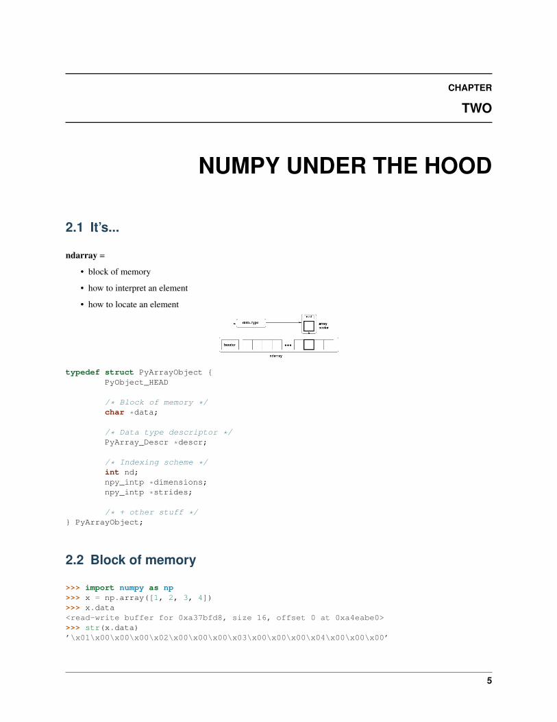
ndarray =

• block of memory

• how to interpret an element

• how to locate an element

typedef struct PyArrayObject {PyObject_HEAD

/* Block of memory */char *data;

/* Data type descriptor */PyArray_Descr *descr;

/* Indexing scheme */int nd;npy_intp *dimensions;npy_intp *strides;

/* + other stuff */} PyArrayObject;

2.2 Block of memory

>>> import numpy as np>>> x = np.array([1, 2, 3, 4])>>> x.data<read-write buffer for 0xa37bfd8, size 16, offset 0 at 0xa4eabe0>>>> str(x.data)’\x01\x00\x00\x00\x02\x00\x00\x00\x03\x00\x00\x00\x04\x00\x00\x00’

5


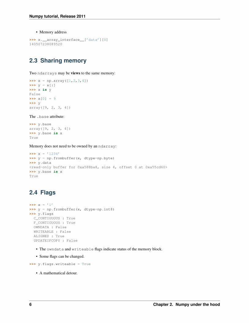
• Memory address

>>> x.__array_interface__[’data’][0]140507238089520

2.3 Sharing memory

Two ndarrays may be views to the same memory:

>>> x = np.array([1,2,3,4])>>> y = x[:]>>> x is yFalse>>> x[0] = 9>>> yarray([9, 2, 3, 4])

The .base attribute:

>>> y.basearray([9, 2, 3, 4])>>> y.base is xTrue

Memory does not need to be owned by an ndarray:

>>> x = ’1234’>>> y = np.frombuffer(x, dtype=np.byte)>>> y.data<read-only buffer for 0xa588ba8, size 4, offset 0 at 0xa55cd60>>>> y.base is xTrue

2.4 Flags

>>> x = ’1’>>> y = np.frombuffer(x, dtype=np.int8)>>> y.flagsC_CONTIGUOUS : TrueF_CONTIGUOUS : TrueOWNDATA : FalseWRITEABLE : FalseALIGNED : TrueUPDATEIFCOPY : False

• The owndata and writeable flags indicate status of the memory block.

• Some flags can be changed.

>>> y.flags.writeable = True

• A mathematical detour.

6 Chapter 2. Numpy under the hood


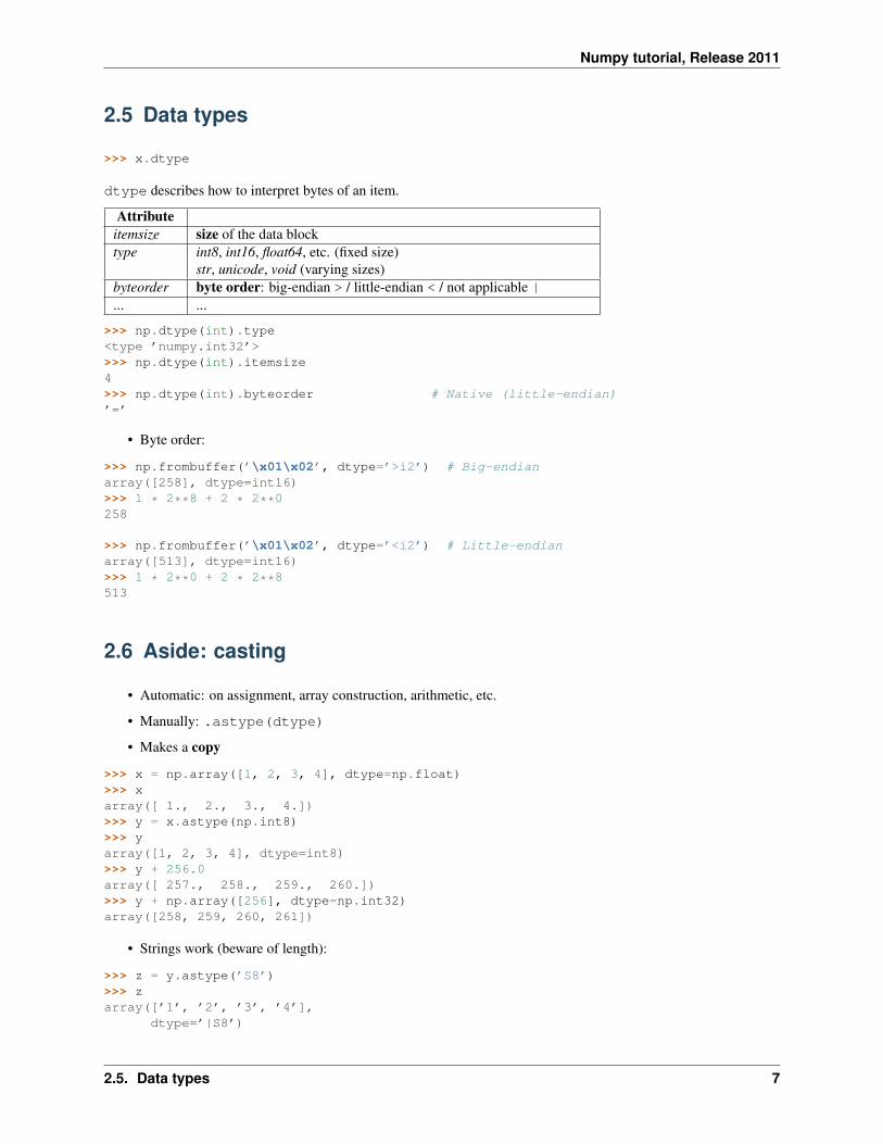
2.5 Data types

>>> x.dtype

dtype describes how to interpret bytes of an item.

Attributeitemsize size of the data blocktype int8, int16, float64, etc. (fixed size)

str, unicode, void (varying sizes)byteorder byte order: big-endian > / little-endian < / not applicable |... ...

>>> np.dtype(int).type<type ’numpy.int32’>>>> np.dtype(int).itemsize4>>> np.dtype(int).byteorder # Native (little-endian)’=’

• Byte order:

>>> np.frombuffer(’\x01\x02’, dtype=’>i2’) # Big-endianarray([258], dtype=int16)>>> 1 * 2**8 + 2 * 2**0258

>>> np.frombuffer(’\x01\x02’, dtype=’<i2’) # Little-endianarray([513], dtype=int16)>>> 1 * 2**0 + 2 * 2**8513

2.6 Aside: casting

• Automatic: on assignment, array construction, arithmetic, etc.

• Manually: .astype(dtype)

• Makes a copy

>>> x = np.array([1, 2, 3, 4], dtype=np.float)>>> xarray([ 1., 2., 3., 4.])>>> y = x.astype(np.int8)>>> yarray([1, 2, 3, 4], dtype=int8)>>> y + 256.0array([ 257., 258., 259., 260.])>>> y + np.array([256], dtype=np.int32)array([258, 259, 260, 261])

• Strings work (beware of length):

>>> z = y.astype(’S8’)>>> zarray([’1’, ’2’, ’3’, ’4’],

dtype=’|S8’)

2.5. Data types 7


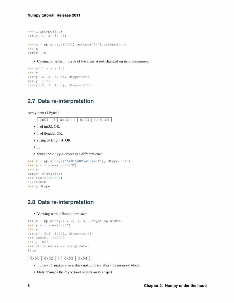
>>> z.astype(int)array([1, 2, 3, 4])

>>> x = np.array([100]).astype(’S2’).astype(int)>>> xarray([10])

• Casting on setitem: dtype of the array is not changed on item assignment

>>> y[:] = y + 1.5>>> yarray([2, 3, 4, 5], dtype=int8)>>> y += 256array([2, 3, 4, 5], dtype=int8)

2.7 Data re-interpretation

Array item (4 bytes)

0x01 || 0x02 || 0x03 || 0x04

• 1 of int32, OR,

• 1 of float32, OR,

• string of length 4, OR,

• ...

• Swap the dtype object to a different one:

>>> x = np.array([’\x01\x02\x03\x04’], dtype=’S4’)>>> y = x.view(np.int32)>>> yarray([67305985])>>> hex(67305985)’0x4030201’>>> y.dtype

2.8 Data re-interpretation

• Viewing with different item size:

>>> x = np.array([1, 2, 3, 4], dtype=np.uint8)>>> y = x.view("<i2")>>> yarray([ 513, 1027], dtype=int16)>>> 0x0201, 0x0403(513, 1027)>>> str(x.data) == str(y.data)True

0x01 0x02 || 0x03 0x04

• .view() makes views, does not copy (or alter) the memory block

• Only changes the dtype (and adjusts array shape)



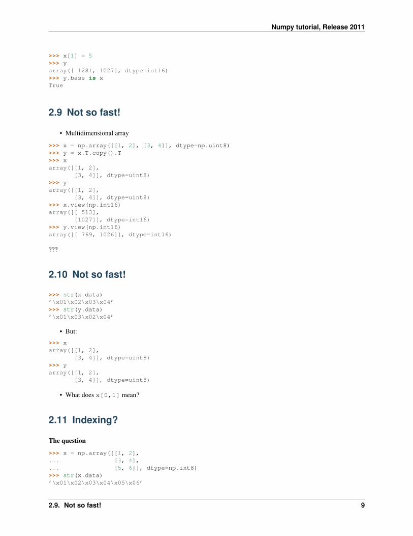
>>> x[1] = 5>>> yarray([ 1281, 1027], dtype=int16)>>> y.base is xTrue

2.9 Not so fast!

• Multidimensional array

>>> x = np.array([[1, 2], [3, 4]], dtype=np.uint8)>>> y = x.T.copy().T>>> xarray([[1, 2],

[3, 4]], dtype=uint8)>>> yarray([[1, 2],

[3, 4]], dtype=uint8)>>> x.view(np.int16)array([[ 513],

[1027]], dtype=int16)>>> y.view(np.int16)array([[ 769, 1026]], dtype=int16)

???

2.10 Not so fast!

>>> str(x.data)’\x01\x02\x03\x04’>>> str(y.data)’\x01\x03\x02\x04’

• But:

>>> xarray([[1, 2],

[3, 4]], dtype=uint8)>>> yarray([[1, 2],

[3, 4]], dtype=uint8)

• What does x[0,1] mean?

2.11 Indexing?

The question

>>> x = np.array([[1, 2],... [3, 4],... [5, 6]], dtype=np.int8)>>> str(x.data)’\x01\x02\x03\x04\x05\x06’

2.9. Not so fast! 9


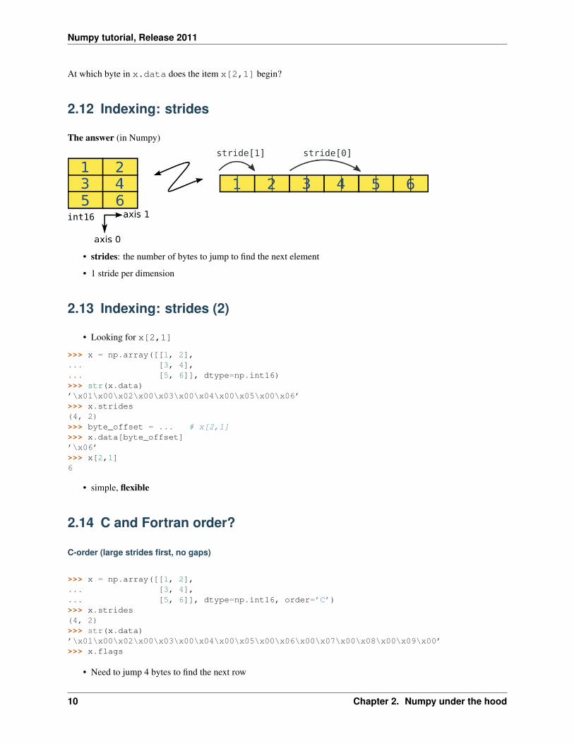
At which byte in x.data does the item x[2,1] begin?

2.12 Indexing: strides

The answer (in Numpy)

• strides: the number of bytes to jump to find the next element

• 1 stride per dimension

2.13 Indexing: strides (2)

• Looking for x[2,1]

>>> x = np.array([[1, 2],... [3, 4],... [5, 6]], dtype=np.int16)>>> str(x.data)’\x01\x00\x02\x00\x03\x00\x04\x00\x05\x00\x06’>>> x.strides(4, 2)>>> byte_offset = ... # x[2,1]>>> x.data[byte_offset]’\x06’>>> x[2,1]6

• simple, flexible

2.14 C and Fortran order?

C-order (large strides first, no gaps)

>>> x = np.array([[1, 2],... [3, 4],... [5, 6]], dtype=np.int16, order=’C’)>>> x.strides(4, 2)>>> str(x.data)’\x01\x00\x02\x00\x03\x00\x04\x00\x05\x00\x06\x00\x07\x00\x08\x00\x09\x00’>>> x.flags

• Need to jump 4 bytes to find the next row



• Need to jump 2 bytes to find the next column

Fortran-order (small strides first, no gaps)

>>> y = np.array(x, order=’F’)>>> y.strides(2, 6)>>> str(y.data)’\x01\x00\x03\x00\x05\x00\x02\x00\x04\x00\x06\x00’>>> y.flags

• Need to jump 2 bytes to find the next row

• Need to jump 6 bytes to find the next column

>>> x == y

2.15 Indexing: Slicing

• All slicing operations: just adjust shape, strides (and data)!

• Never need to make copies

>>> x = np.array([1, 2, 3, 4, 5, 6], dtype=np.int32)>>> y = x[::-1]>>> yarray([6, 5, 4, 3, 2, 1])>>> y.strides(-4,)

>>> y = x[2:]>>> y.__array_interface__[’data’][0] - x.__array_interface__[’data’][0]8

>>> x = np.zeros((10, 10, 10), dtype=np.float)>>> x.strides(800, 80, 8)>>> x[::2,::3,::4].strides(1600, 240, 32)

2.16 Manual stride manipulation

>>> from numpy.lib.stride_tricks import as_strided>>> as_strided?

>>> x = np.array([1, 2, 3, 4], dtype=np.int16)>>> x[::2]>>> x[::2].strides(4,)>>> as_strided(x, strides=(4,), shape=(2,))array([1, 3], dtype=int16)

2.15. Indexing: Slicing 11


2.17 More strides: diagonals

>>> x = np.array([[1, 2, 3],... [4, 5, 6],... [7, 8, 9]], dtype=np.int32)

Q: Pick the diagonal entries

>>> x_diag = as_strided(x, shape=(3,), strides=((3+1)*x.itemsize,))>>> x_diagarray([1, 5, 9])

2.18 More strides: A small mistake...

Bad:

>>> x_diag = as_strided(x, shape=(3e6,), strides=((3+1)*x.itemsize,))>>> x_diag += 9Segmentation fault (core dumped)

Even worse:

>>> x_diag = as_strided(x, shape=(4,), strides=((3+1)*x.itemsize,))>>> x_diag += 9>>> # <-- No segmentation fault!

Warning: as_strided does not do any sanity checks...Good only for:

• Demonstrating strides.• For writing functions that do a specific thing (and make the checks!)

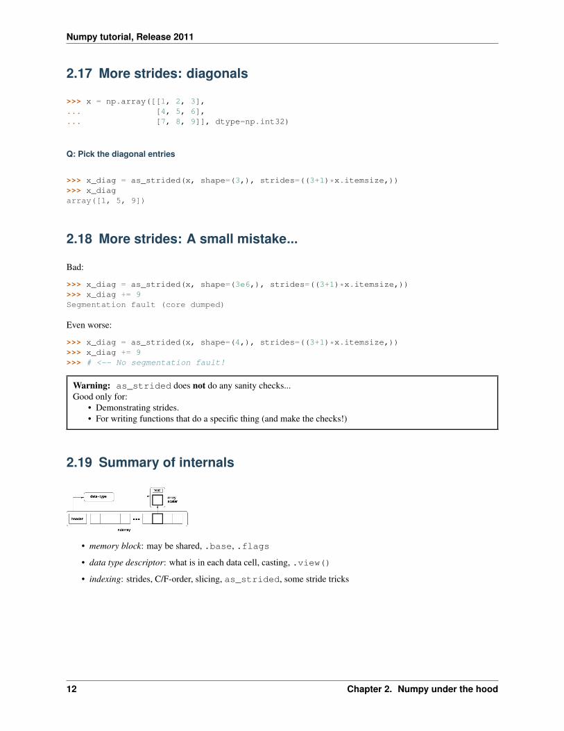
2.19 Summary of internals

• memory block: may be shared, .base, .flags

• data type descriptor: what is in each data cell, casting, .view()

• indexing: strides, C/F-order, slicing, as_strided, some stride tricks


CHAPTER

THREE

EVERYDAY FEATURES:BROADCASTING

3.1 Scalars

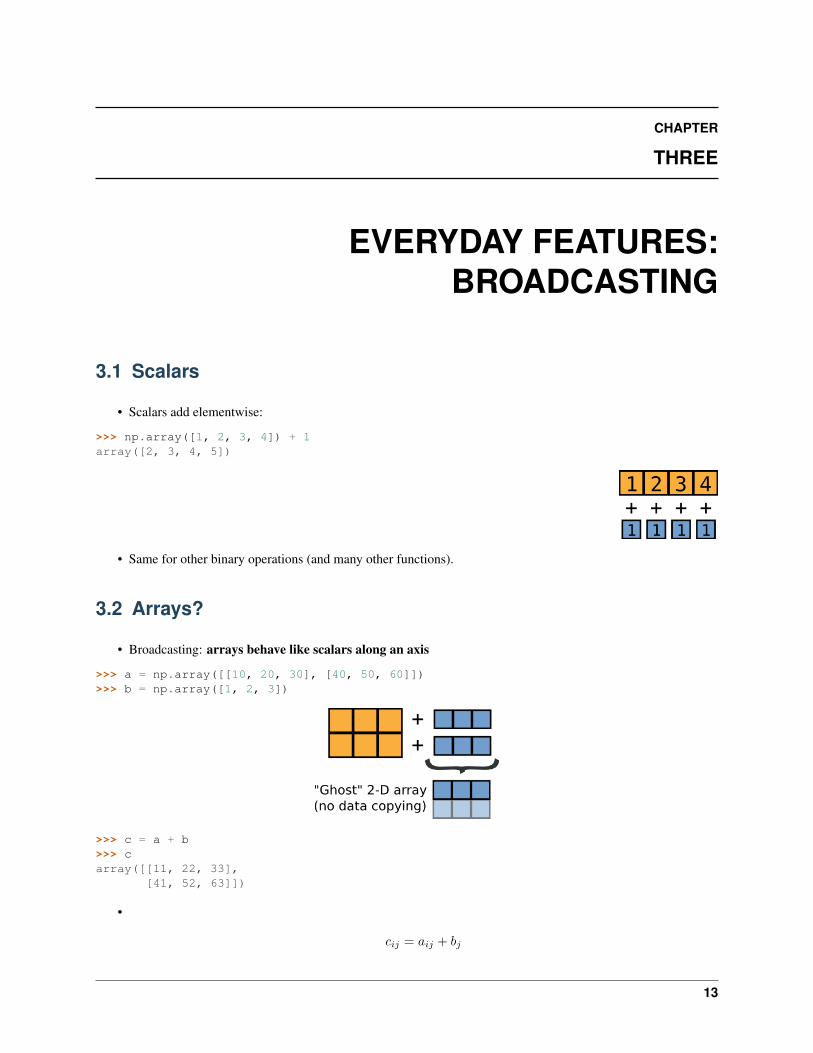
• Scalars add elementwise:

>>> np.array([1, 2, 3, 4]) + 1array([2, 3, 4, 5])

• Same for other binary operations (and many other functions).

3.2 Arrays?

• Broadcasting: arrays behave like scalars along an axis

>>> a = np.array([[10, 20, 30], [40, 50, 60]])>>> b = np.array([1, 2, 3])

>>> c = a + b>>> carray([[11, 22, 33],

[41, 52, 63]])

•

cij = aij + bj

13


>>> a[1,2] + b[2] == (a + b)[1,2]True

3.3 Shape matching

• Same number of dimensions:

>>> a = np.array([[10, 20, 30], [40, 50, 60]])>>> b = np.array([1, 2, 3])[np.newaxis,:]>>> c = a + b>>> a.shape(2, 3)>>> b.shape(1, 3)>>> c.shape(2, 3)

Shape arithmetic:

(2, 3) (2, 3)(1, 3) (3,) <-- behaves as scalar for axis=0

-------- --------(2, 3) (2, 3)

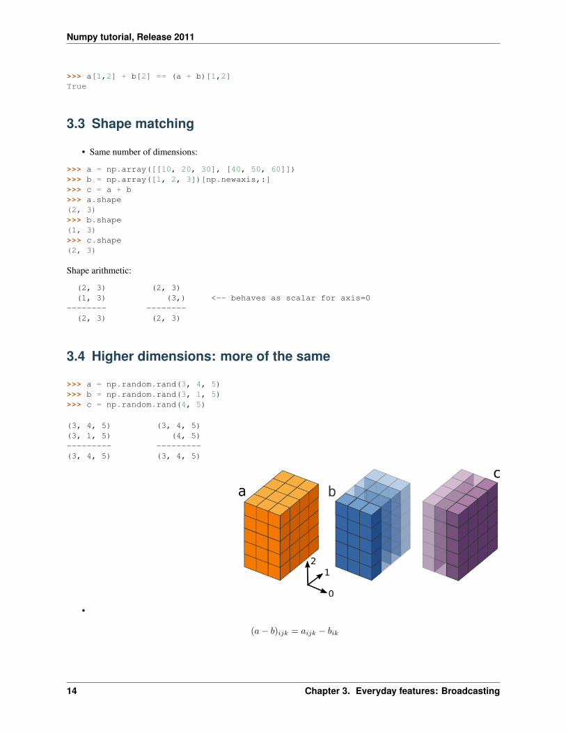
3.4 Higher dimensions: more of the same

>>> a = np.random.rand(3, 4, 5)>>> b = np.random.rand(3, 1, 5)>>> c = np.random.rand(4, 5)

(3, 4, 5) (3, 4, 5)(3, 1, 5) (4, 5)--------- ---------(3, 4, 5) (3, 4, 5)

•

(a− b)ijk = aijk − bik

14 Chapter 3. Everyday features: Broadcasting


>>> (a[1,3,2] - b[1,0,2]) == (a - b)[1,3,2]True

•

(a− c)ijk = aijk − cjk

>>> (a[1,3,2] - c[3,2]) == (a - c)[1,3,2]True

3.5 Common uses (1/3)

• Evaluating something on a grid:

>>> x, y = np.arange(5), np.arange(5)>>> distance = np.sqrt(x**2 + y[:, np.newaxis]**2)>>> distancearray([[ 0. , 1. , 2. , 3. , 4. ],

[ 1. , 1.41421356, 2.23606798, 3.16227766, 4.12310563],[ 2. , 2.23606798, 2.82842712, 3.60555128, 4.47213595],[ 3. , 3.16227766, 3.60555128, 4.24264069, 5. ],[ 4. , 4.12310563, 4.47213595, 5. , 5.65685425]])


• np.ogrid

>>> x, y = np.ogrid[0:5, 0:5]>>> x.shape, y.shape((5, 1), (1, 5))>>> distance = np.sqrt(x**2 + y**2)

• np.ix_


• Tensor operations

Example: many matrix products for small matrices

>>> R = np.random.rand(3, 3, 2000) # 2000 of 3x3 matrices>>> Z = np.random.rand(3, 3, 2000)

Compute R_k.dot(Z_k) for each 3x3 matrices R_k and Z_k in R, Z

(RZ)ijk =∑

p RipkZpjk

i p j kR : : na :Z na : : :---------------------RZ : sum : :

3.5. Common uses (1/3) 15


>>> RZ = (R[:,:,newaxis,:] * Z[newaxis,:,:,:]).sum(axis=1)

• ... or einsum (Numpy >= 1.6; faster)

>>> ...

3.8 Explicit broadcasting

• Explicitly broadcast arrays are sometimes useful:

>>> x = np.array([10, 20, 30, 40]).reshape(1, 4)>>> y = np.array([1, 2, 3]).reshape(3, 1)

>>> x2, y2 = np.broadcast_arrays(x, y)>>> x2array([[10, 20, 30, 40],

[10, 20, 30, 40],[10, 20, 30, 40]])

>>> y2array([[1, 1, 1, 1],

[2, 2, 2, 2],[3, 3, 3, 3]])

• They’re views?

>>> x[0,0] = -1>>> x2array([[-1, 20, 30, 40],

[-1, 20, 30, 40],[-1, 20, 30, 40]])

• Strides?

>>> ...

3.9 Ghost arrays

• Internally, broadcasting uses 0-strides

>>> x = np.array([10, 20, 30, 40]).reshape(1, 4)>>> y = np.array([1, 2, 3]).reshape(3, 1)

>>> from numpy.lib.stride_tricks import as_strided

>>> x2 = as_strided(x, strides=(...), shape=(3, 4)) # No copying!>>> x2array([[10, 20, 30, 40],

[10, 20, 30, 40],[10, 20, 30, 40]])

>>> y2 = as_strided(y, strides=(...), shape=(3, 4))>>> y2array([[1, 1, 1, 1],

[2, 2, 2, 2],[3, 3, 3, 3]])



• Indexing vs. 0-strides

>>> byte_offset = ...

3.9. Ghost arrays 17

CHAPTER

FOUR

EVERYDAY FEATURES: FANCYINDEXING

4.1 Boolean masks

>>> a = np.array([1, 2, 3, 4])>>> a > 2array([False, False, True, True], dtype=bool)>>> a[a > 2]array([3, 4])

• Always a copy (cannot do with strides)

>>> a[a > 2][0] = -1 # OBS!>>> aarray([1, 2, 3, 4])

• Assignment works:

>>> a[a > 2] = -1>>> aarray([ 1, 2, -1, -1])

4.2 Boolean masks, ndim > 1

• 1-D masks

>>> a = np.arange(4*5).reshape(4, 5)>>> aarray([[ 0, 1, 2, 3, 4],

[ 5, 6, 7, 8, 9],[10, 11, 12, 13, 14],[15, 16, 17, 18, 19]])

• Extract rows

>>> a[np.array([True,False,False,True])]array([[ 0, 1, 2, 3, 4],

[15, 16, 97, 98, 99]])

• Extract columns

19


>>> a[:, np.array([True,True,False,False,True])]array([[ 0, 1, 4],

[ 5, 6, 9],[10, 11, 14],[15, 16, 99]])

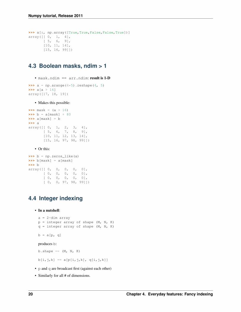
4.3 Boolean masks, ndim > 1

• mask.ndim == arr.ndim: result is 1-D

>>> a = np.arange(4*5).reshape(4, 5)>>> a[a > 16]array([17, 18, 19])

• Makes this possible:

>>> mask = (a > 16)>>> b = a[mask] + 80>>> a[mask] = b>>> aarray([[ 0, 1, 2, 3, 4],

[ 5, 6, 7, 8, 9],[10, 11, 12, 13, 14],[15, 16, 97, 98, 99]])

• Or this:

>>> b = np.zeros_like(a)>>> b[mask] = a[mask]>>> barray([[ 0, 0, 0, 0, 0],

[ 0, 0, 0, 0, 0],[ 0, 0, 0, 0, 0],[ 0, 0, 97, 98, 99]])

4.4 Integer indexing

• In a nutshell:

a = 2-dim arrayp = integer array of shape (M, N, K)q = integer array of shape (M, N, K)

b = a[p, q]

produces b:

b.shape == (M, N, K)

b[i,j,k] == a[p[i,j,k], q[i,j,k]]

• p and q are broadcast first (against each other)

• Similarly for all # of dimensions.

20 Chapter 4. Everyday features: Fancy indexing


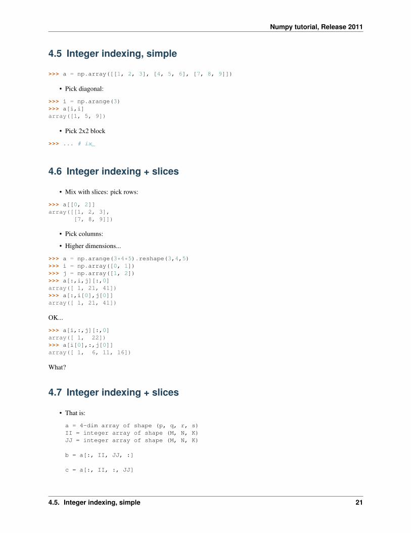
4.5 Integer indexing, simple

>>> a = np.array([[1, 2, 3], [4, 5, 6], [7, 8, 9]])

• Pick diagonal:

>>> i = np.arange(3)>>> a[i,i]array([1, 5, 9])

• Pick 2x2 block

>>> ... # ix_

4.6 Integer indexing + slices

• Mix with slices: pick rows:

>>> a[[0, 2]]array([[1, 2, 3],

[7, 8, 9]])

• Pick columns:

• Higher dimensions...

>>> a = np.arange(3*4*5).reshape(3,4,5)>>> i = np.array([0, 1])>>> j = np.array([1, 2])>>> a[:,i,j][:,0]array([ 1, 21, 41])>>> a[:,i[0],j[0]]array([ 1, 21, 41])

OK...

>>> a[i,:,j][:,0]array([ 1, 22])>>> a[i[0],:,j[0]]array([ 1, 6, 11, 16])

What?

4.7 Integer indexing + slices

• That is:

a = 4-dim array of shape (p, q, r, s)II = integer array of shape (M, N, K)JJ = integer array of shape (M, N, K)

b = a[:, II, JJ, :]

c = a[:, II, :, JJ]

4.5. Integer indexing, simple 21


produces b, c:

b.shape == (p, M, N, K, q)

b[i,j,k,l,m] == a[i, II[j,k,l], JJ[j,k,l], m]

c.shape == (M, N, K, p, q)

c[i,j,k,l,m] == a[l, II[i,j,k], m, JJ[i,j,k]]

• Fancy indices are next to each other: fancy axes go to the same position

• Otherwise, fancy axes go first

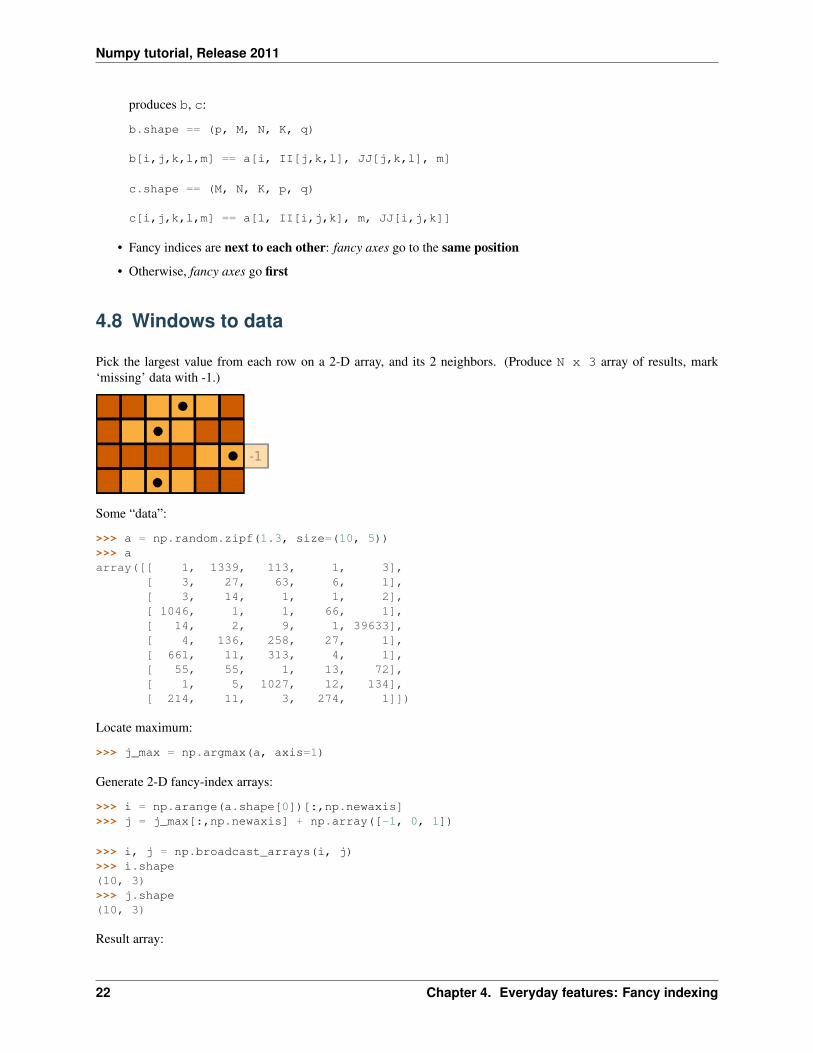
4.8 Windows to data

Pick the largest value from each row on a 2-D array, and its 2 neighbors. (Produce N x 3 array of results, mark‘missing’ data with -1.)

Some “data”:

>>> a = np.random.zipf(1.3, size=(10, 5))>>> aarray([[ 1, 1339, 113, 1, 3],

[ 3, 27, 63, 6, 1],[ 3, 14, 1, 1, 2],[ 1046, 1, 1, 66, 1],[ 14, 2, 9, 1, 39633],[ 4, 136, 258, 27, 1],[ 661, 11, 313, 4, 1],[ 55, 55, 1, 13, 72],[ 1, 5, 1027, 12, 134],[ 214, 11, 3, 274, 1]])

Locate maximum:

>>> j_max = np.argmax(a, axis=1)

Generate 2-D fancy-index arrays:

>>> i = np.arange(a.shape[0])[:,np.newaxis]>>> j = j_max[:,np.newaxis] + np.array([-1, 0, 1])

>>> i, j = np.broadcast_arrays(i, j)>>> i.shape(10, 3)>>> j.shape(10, 3)

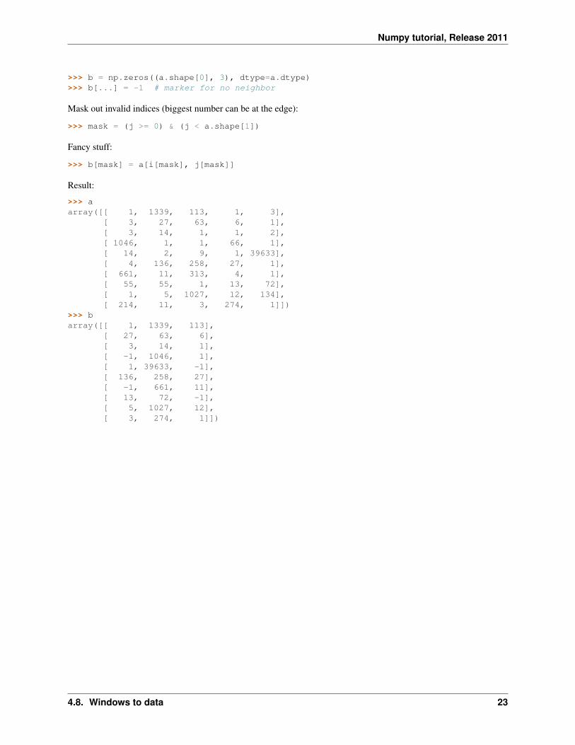
Result array:



>>> b = np.zeros((a.shape[0], 3), dtype=a.dtype)>>> b[...] = -1 # marker for no neighbor

Mask out invalid indices (biggest number can be at the edge):

>>> mask = (j >= 0) & (j < a.shape[1])

Fancy stuff:

>>> b[mask] = a[i[mask], j[mask]]

Result:

>>> aarray([[ 1, 1339, 113, 1, 3],

[ 3, 27, 63, 6, 1],[ 3, 14, 1, 1, 2],[ 1046, 1, 1, 66, 1],[ 14, 2, 9, 1, 39633],[ 4, 136, 258, 27, 1],[ 661, 11, 313, 4, 1],[ 55, 55, 1, 13, 72],[ 1, 5, 1027, 12, 134],[ 214, 11, 3, 274, 1]])

>>> barray([[ 1, 1339, 113],

[ 27, 63, 6],[ 3, 14, 1],[ -1, 1046, 1],[ 1, 39633, -1],[ 136, 258, 27],[ -1, 661, 11],[ 13, 72, -1],[ 5, 1027, 12],[ 3, 274, 1]])

4.8. Windows to data 23

CHAPTER

FIVE

EVERYDAY FEATURES: STRUCTUREDDATA TYPES

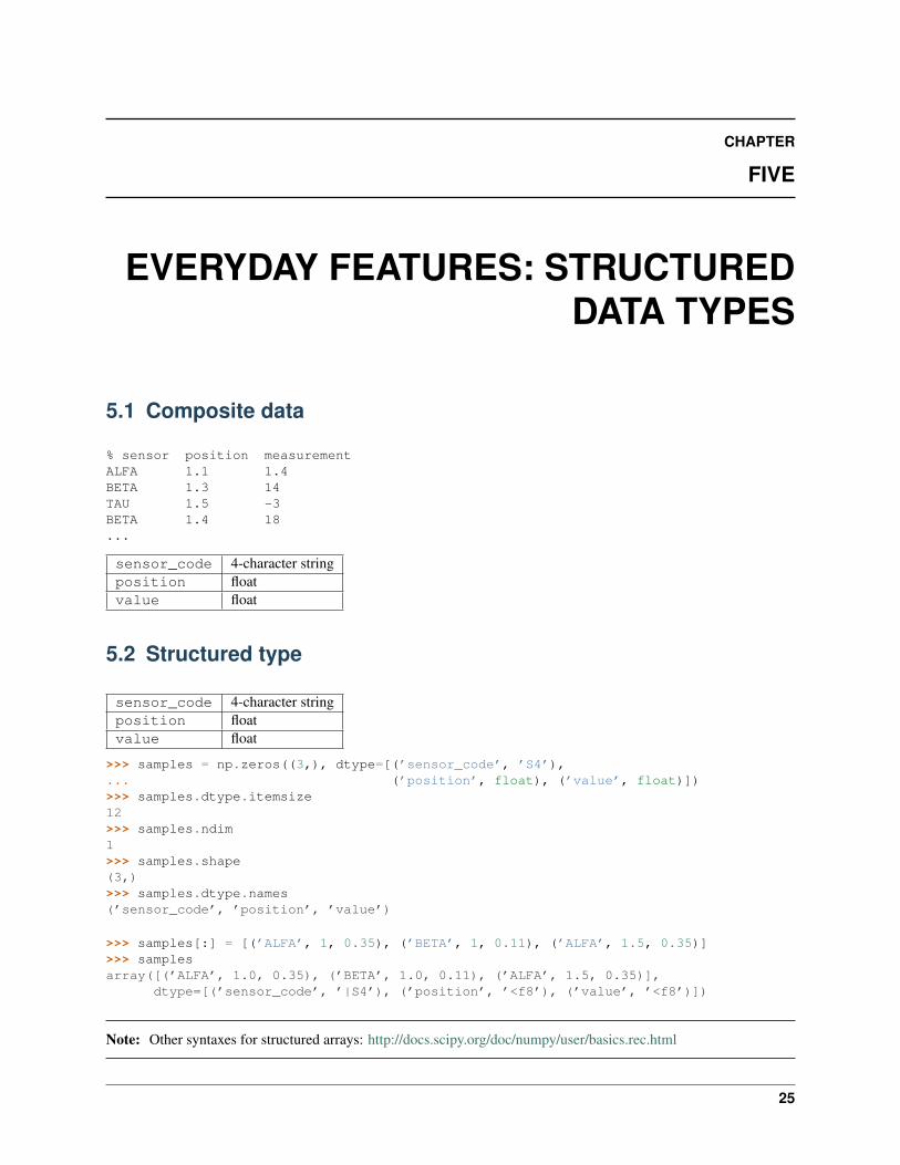
5.1 Composite data

% sensor position measurementALFA 1.1 1.4BETA 1.3 14TAU 1.5 -3BETA 1.4 18...

sensor_code 4-character stringposition floatvalue float

5.2 Structured type

sensor_code 4-character stringposition floatvalue float

>>> samples = np.zeros((3,), dtype=[(’sensor_code’, ’S4’),... (’position’, float), (’value’, float)])>>> samples.dtype.itemsize12>>> samples.ndim1>>> samples.shape(3,)>>> samples.dtype.names(’sensor_code’, ’position’, ’value’)

>>> samples[:] = [(’ALFA’, 1, 0.35), (’BETA’, 1, 0.11), (’ALFA’, 1.5, 0.35)]>>> samplesarray([(’ALFA’, 1.0, 0.35), (’BETA’, 1.0, 0.11), (’ALFA’, 1.5, 0.35)],

dtype=[(’sensor_code’, ’|S4’), (’position’, ’<f8’), (’value’, ’<f8’)])

Note: Other syntaxes for structured arrays: http://docs.scipy.org/doc/numpy/user/basics.rec.html

25

http://docs.scipy.org/doc/numpy/user/basics.rec.html


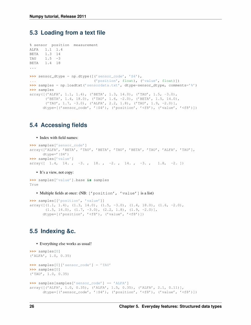
5.3 Loading from a text file

% sensor position measurementALFA 1.1 1.4BETA 1.3 14TAU 1.5 -3BETA 1.4 18...

>>> sensor_dtype = np.dtype([(’sensor_code’, ’S4’),... (’position’, float), (’value’, float)])>>> samples = np.loadtxt(’sensordata.txt’, dtype=sensor_dtype, comments=’%’)>>> samplesarray([(’ALFA’, 1.1, 1.4), (’BETA’, 1.3, 14.0), (’TAU’, 1.5, -3.0),

(’BETA’, 1.4, 18.0), (’TAU’, 1.6, -2.0), (’BETA’, 1.5, 14.0),(’TAU’, 1.7, -3.0), (’ALFA’, 2.2, 1.8), (’TAU’, 1.9, -2.0)],


5.4 Accessing fields

• Index with field names:

>>> samples[’sensor_code’]array([’ALFA’, ’BETA’, ’TAU’, ’BETA’, ’TAU’, ’BETA’, ’TAU’, ’ALFA’, ’TAU’],

dtype=’|S4’)>>> samples[’value’]array([ 1.4, 14. , -3. , 18. , -2. , 14. , -3. , 1.8, -2. ])

• It’s a view, not copy:

>>> samples[’value’].base is samplesTrue

• Multiple fields at once: (NB: [’position’, ’value’] is a list)

>>> samples[[’position’, ’value’]]array([(1.1, 1.4), (1.3, 14.0), (1.5, -3.0), (1.4, 18.0), (1.6, -2.0),

(1.5, 14.0), (1.7, -3.0), (2.2, 1.8), (1.9, -2.0)],dtype=[(’position’, ’<f8’), (’value’, ’<f8’)])

5.5 Indexing &c.

• Everything else works as usual!

>>> samples[0](’ALFA’, 1.0, 0.35)

>>> samples[0][’sensor_code’] = ’TAU’>>> samples[0](’TAU’, 1.0, 0.35)

>>> samples[samples[’sensor_code’] == ’ALFA’]array([(’ALFA’, 1.0, 0.35), (’ALFA’, 1.5, 0.35), (’ALFA’, 2.1, 0.11)],


26 Chapter 5. Everyday features: Structured data types


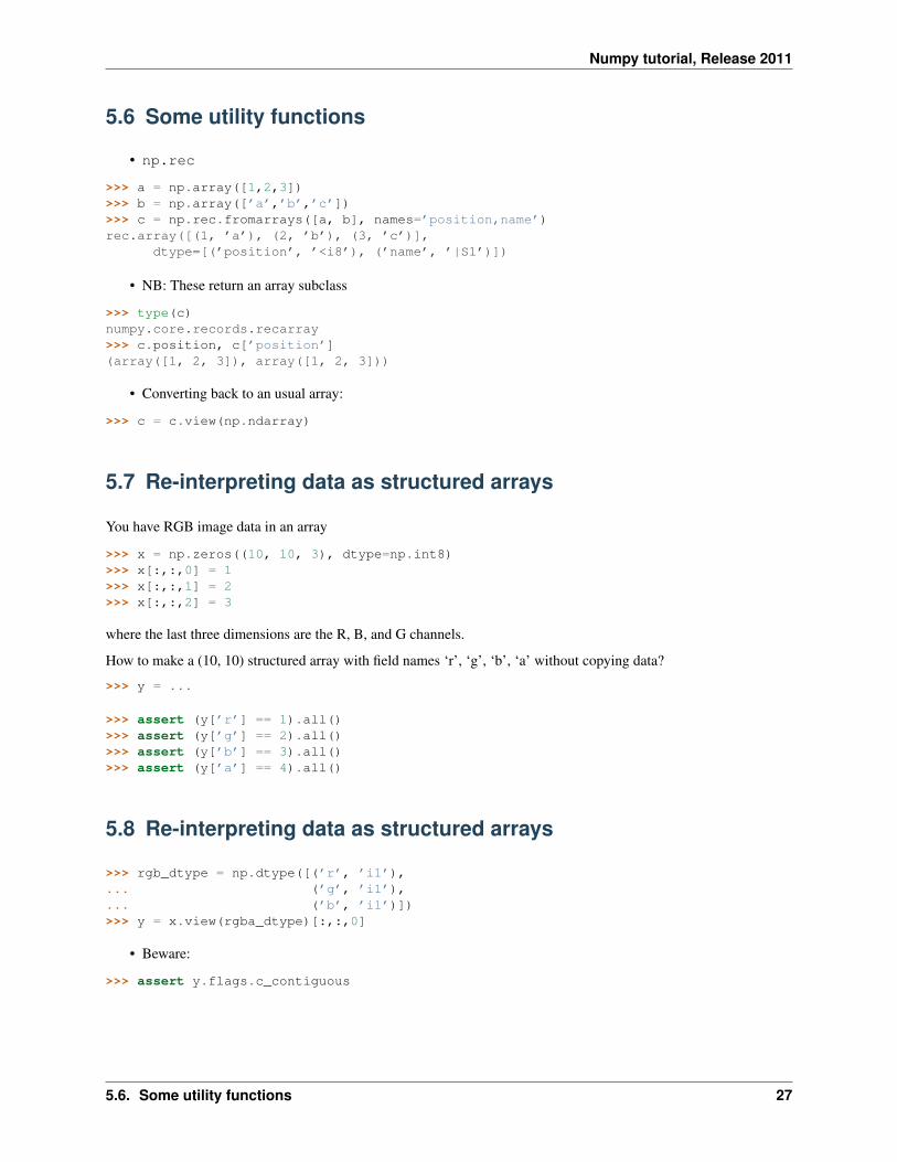
5.6 Some utility functions

• np.rec

>>> a = np.array([1,2,3])>>> b = np.array([’a’,’b’,’c’])>>> c = np.rec.fromarrays([a, b], names=’position,name’)rec.array([(1, ’a’), (2, ’b’), (3, ’c’)],

dtype=[(’position’, ’<i8’), (’name’, ’|S1’)])

• NB: These return an array subclass

>>> type(c)numpy.core.records.recarray>>> c.position, c[’position’](array([1, 2, 3]), array([1, 2, 3]))

• Converting back to an usual array:

>>> c = c.view(np.ndarray)

5.7 Re-interpreting data as structured arrays

You have RGB image data in an array

>>> x = np.zeros((10, 10, 3), dtype=np.int8)>>> x[:,:,0] = 1>>> x[:,:,1] = 2>>> x[:,:,2] = 3

where the last three dimensions are the R, B, and G channels.

How to make a (10, 10) structured array with field names ‘r’, ‘g’, ‘b’, ‘a’ without copying data?

>>> y = ...

>>> assert (y[’r’] == 1).all()>>> assert (y[’g’] == 2).all()>>> assert (y[’b’] == 3).all()>>> assert (y[’a’] == 4).all()

5.8 Re-interpreting data as structured arrays

>>> rgb_dtype = np.dtype([(’r’, ’i1’),... (’g’, ’i1’),... (’b’, ’i1’)])>>> y = x.view(rgba_dtype)[:,:,0]

• Beware:

>>> assert y.flags.c_contiguous

5.6. Some utility functions 27


28 Chapter 5. Everyday features: Structured data types

CHAPTER

SIX

SUMMARY

• Internals

Indexing, slicing, strides, etc.

• Broadcasting

• Fancy indexing

• Structured arrays

29


30 Chapter 6. Summary

CHAPTER

SEVEN

EXERCISES

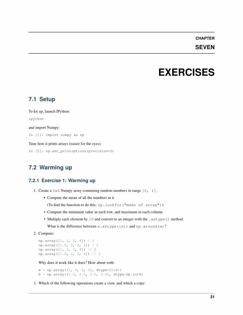
7.1 Setup

To kit up, launch IPython:

ipython

and import Numpy:

In [1]: import numpy as np

Tune how it prints arrays (easier for the eyes):

In [2]: np.set_printoptions(precision=3)

7.2 Warming up

7.2.1 Exercise 1: Warming up

1. Create a 5x6 Numpy array containing random numbers in range [0, 1].

• Compute the mean of all the numbers in it

(To find the function to do this: np.lookfor("mean of array"))

• Compute the minimum value in each row, and maximum in each column

• Multiply each element by 10 and convert to an integer with the .astype() method.

What is the difference between a.astype(int) and np.around(a)?

2. Compare:

np.array([1, 2, 3, 4]) / 2np.array([1.0, 2, 3, 4]) / 2np.array([1, 2, 3, 4]) // 2np.array([1.0, 2, 3, 4]) // 2

Why does it work like it does? How about with:

a = np.array([1, 2, 3, 4], dtype=float)b = np.array([1.0, 2.0, 3.0, 4.0], dtype=np.int8)

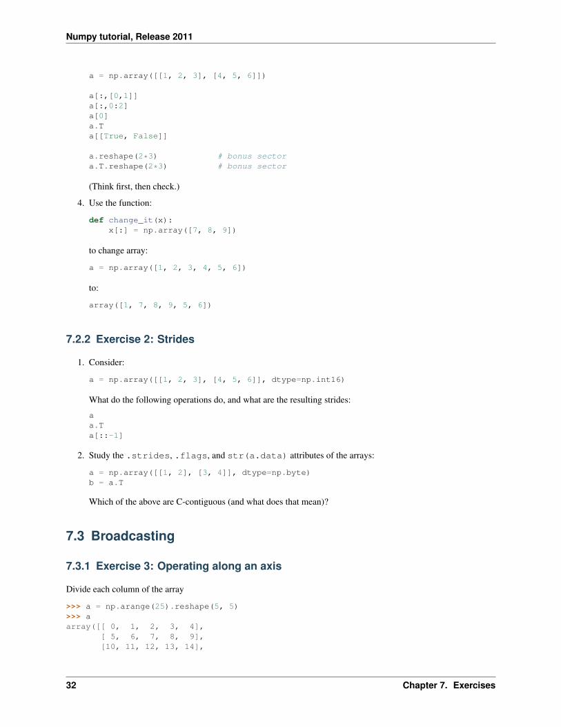
3. Which of the following operations create a view, and which a copy:

31


a = np.array([[1, 2, 3], [4, 5, 6]])

a[:,[0,1]]a[:,0:2]a[0]a.Ta[[True, False]]

a.reshape(2*3) # bonus sectora.T.reshape(2*3) # bonus sector

(Think first, then check.)

4. Use the function:

def change_it(x):x[:] = np.array([7, 8, 9])

to change array:

a = np.array([1, 2, 3, 4, 5, 6])

to:

array([1, 7, 8, 9, 5, 6])

7.2.2 Exercise 2: Strides

1. Consider:

a = np.array([[1, 2, 3], [4, 5, 6]], dtype=np.int16)

What do the following operations do, and what are the resulting strides:

aa.Ta[::-1]

2. Study the .strides, .flags, and str(a.data) attributes of the arrays:

a = np.array([[1, 2], [3, 4]], dtype=np.byte)b = a.T

Which of the above are C-contiguous (and what does that mean)?

7.3 Broadcasting

7.3.1 Exercise 3: Operating along an axis

Divide each column of the array

>>> a = np.arange(25).reshape(5, 5)>>> aarray([[ 0, 1, 2, 3, 4],

[ 5, 6, 7, 8, 9],[10, 11, 12, 13, 14],

32 Chapter 7. Exercises


[15, 16, 17, 18, 19],[20, 21, 22, 23, 24]])

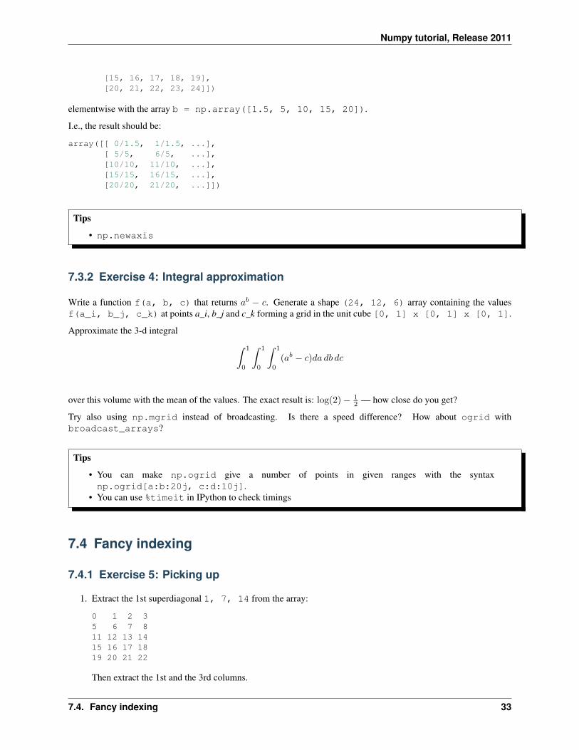
elementwise with the array b = np.array([1.5, 5, 10, 15, 20]).

I.e., the result should be:

array([[ 0/1.5, 1/1.5, ...],[ 5/5, 6/5, ...],[10/10, 11/10, ...],[15/15, 16/15, ...],[20/20, 21/20, ...]])

Tips

• np.newaxis

7.3.2 Exercise 4: Integral approximation

Write a function f(a, b, c) that returns ab − c. Generate a shape (24, 12, 6) array containing the valuesf(a_i, b_j, c_k) at points a_i, b_j and c_k forming a grid in the unit cube [0, 1] x [0, 1] x [0, 1].

Approximate the 3-d integral ∫ 1

0

∫ 1

0

∫ 1

0

(ab − c)da db dc

over this volume with the mean of the values. The exact result is: log(2)− 12 — how close do you get?

Try also using np.mgrid instead of broadcasting. Is there a speed difference? How about ogrid withbroadcast_arrays?

Tips

• You can make np.ogrid give a number of points in given ranges with the syntaxnp.ogrid[a:b:20j, c:d:10j].

• You can use %timeit in IPython to check timings

7.4 Fancy indexing

7.4.1 Exercise 5: Picking up

1. Extract the 1st superdiagonal 1, 7, 14 from the array:

0 1 2 35 6 7 811 12 13 1415 16 17 1819 20 21 22

Then extract the 1st and the 3rd columns.

7.4. Fancy indexing 33


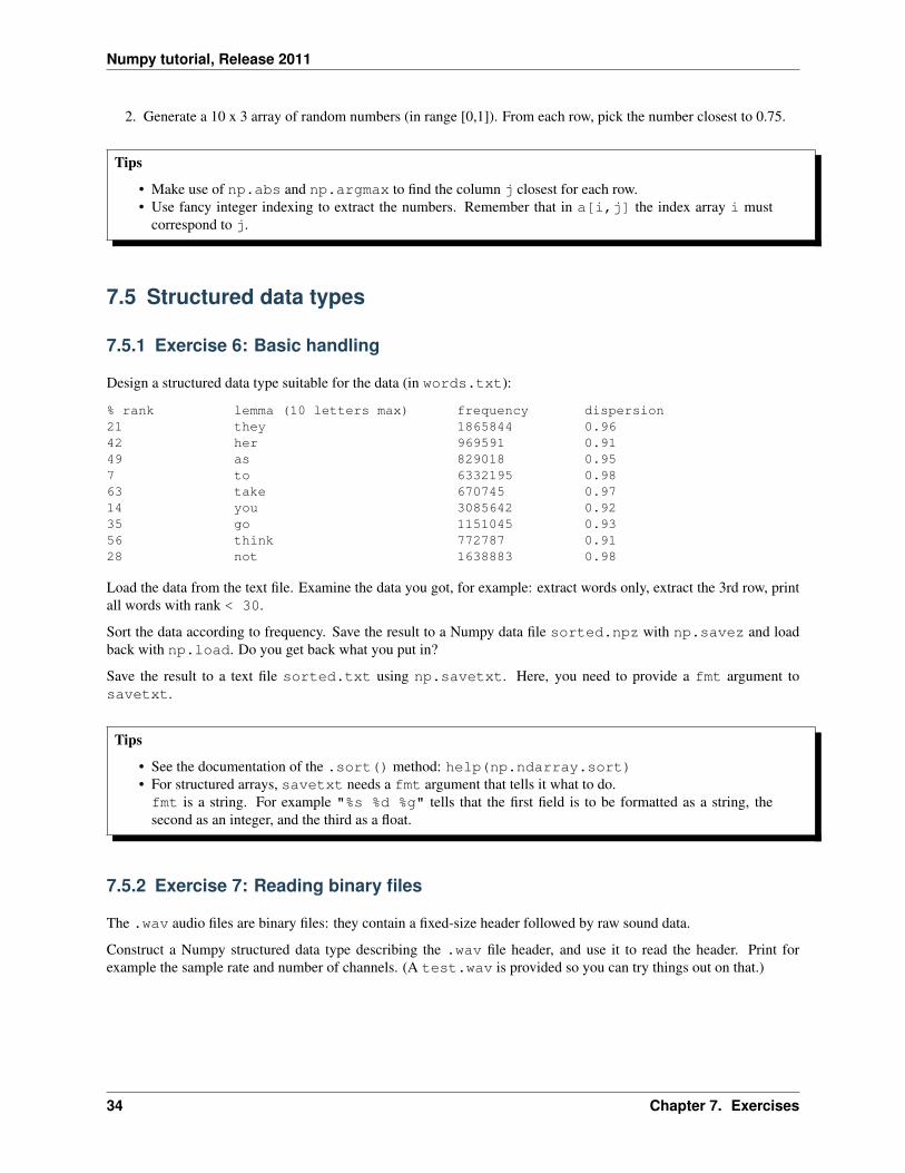
2. Generate a 10 x 3 array of random numbers (in range [0,1]). From each row, pick the number closest to 0.75.

Tips

• Make use of np.abs and np.argmax to find the column j closest for each row.• Use fancy integer indexing to extract the numbers. Remember that in a[i,j] the index array i must

correspond to j.

7.5 Structured data types

7.5.1 Exercise 6: Basic handling

Design a structured data type suitable for the data (in words.txt):

% rank lemma (10 letters max) frequency dispersion21 they 1865844 0.9642 her 969591 0.9149 as 829018 0.957 to 6332195 0.9863 take 670745 0.9714 you 3085642 0.9235 go 1151045 0.9356 think 772787 0.9128 not 1638883 0.98

Load the data from the text file. Examine the data you got, for example: extract words only, extract the 3rd row, printall words with rank < 30.

Sort the data according to frequency. Save the result to a Numpy data file sorted.npz with np.savez and loadback with np.load. Do you get back what you put in?

Save the result to a text file sorted.txt using np.savetxt. Here, you need to provide a fmt argument tosavetxt.

Tips

• See the documentation of the .sort() method: help(np.ndarray.sort)• For structured arrays, savetxt needs a fmt argument that tells it what to do.fmt is a string. For example "%s %d %g" tells that the first field is to be formatted as a string, thesecond as an integer, and the third as a float.

7.5.2 Exercise 7: Reading binary files

The .wav audio files are binary files: they contain a fixed-size header followed by raw sound data.

Construct a Numpy structured data type describing the .wav file header, and use it to read the header. Print forexample the sample rate and number of channels. (A test.wav is provided so you can try things out on that.)



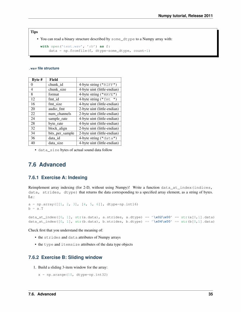
Tips

• You can read a binary structure described by some_dtype to a Numpy array with:

with open(’test.wav’, ’rb’) as f:data = np.fromfile(f, dtype=some_dtype, count=1)

.wav file structure

Byte # Field0 chunk_id 4-byte string ("RIFF")4 chunk_size 4-byte uint (little-endian)8 format 4-byte string ("WAVE")12 fmt_id 4-byte string ("fmt ")16 fmt_size 4-byte uint (little-endian)20 audio_fmt 2-byte uint (little-endian)22 num_channels 2-byte uint (little-endian)24 sample_rate 4-byte uint (little-endian)28 byte_rate 4-byte uint (little-endian)32 block_align 2-byte uint (little-endian)34 bits_per_sample 2-byte uint (little-endian)36 data_id 4-byte string ("data")40 data_size 4-byte uint (little-endian)

• data_size bytes of actual sound data follow

7.6 Advanced

7.6.1 Exercise A: Indexing

Reimplement array indexing (for 2-D, without using Numpy)! Write a function data_at_index(indices,data, strides, dtype) that returns the data corresponding to a specified array element, as a string of bytes.I.e.:

a = np.array([[1, 2, 3], [4, 5, 6]], dtype=np.int16)b = a.T

data_at_index([0, 1], str(a.data), a.strides, a.dtype) == ’\x02\x00’ == str(a[0,1].data)data_at_index([0, 1], str(b.data), b.strides, b.dtype) == ’\x04\x00’ == str(b[0,1].data)

Check first that you understand the meaning of:

• the strides and data attributes of Numpy arrays

• the type and itemsize attributes of the data type objects

7.6.2 Exercise B: Sliding window

1. Build a sliding 3-item window for the array:

x = np.arange(10, dtype=np.int32)

7.6. Advanced 35


The aim is to get an array:

array([[0, 1, 2],[1, 2, 3],[2, 3, 4],[3, 4, 5],[4, 5, 6],[5, 6, 7],[6, 7, 8],[7, 8, 9]], dtype=int32)

without making copies (so that it is fast). The trick is a stride trick:

from numpy.lib.stride_tricks import as_stridedstrides = ...y = as_strided(x, shape=(8, 3), strides=strides)

2. Use the same trick to compute the 5 x 5 median filter of an image. For each pixel, compute the median of the5 x 5 block of pixels surrounding it.

The median filter provides a degree of denoising similarly to a gaussian blur, but it preserves sharp edges better.

>>> import scipy>>> import matplotlib.pyplot as plt

Noisy image

>>> img = scipy.lena() # A standard test image for image processing>>> img += 0.8 * img.std() * np.random.rand(*img.shape)>>> plt.imshow(img)

0 100 200 300 400 500

0

100

200

300

400

500

Prepare the sliding window

>>> assert img.flags.c_contiguous # Important!

>>> window_size = 5>>> shape = ... # Careful, no out-of-bounds access...>>> strides = ...

>>> img_window = as_strided(...)

Denoise!

>>> img_median = np.median(img_window.reshape(..., window_size*window_size), axis=...)>>> plt.imshow(img_median)>>> plt.gray()>>> plt.imsave(’sharpened.png’, img_median)

Note:

• Above, the .reshape() makes a copy (why?).

• Scipy has an implementation for the median filter in scipy.ndimage, with more features.



Extra: Visit the factory

We don’t yet have a rolling_window function in Numpy that would make the above easier. We, however, do havea contributed implementation that is discussed here:

https://github.com/numpy/numpy/pull/31

Can you extend the version posted by Warren to make N-dimensional windows, or think of any other features such afunction would need to have? (If yes, just ask me how to contribute your stuff.)

7.6.3 Exercise C: Menger sponge

Generate an approximation to the Menger sponge by creating a 3-D Numpy array filled with 1, and drilling holes to itwith slicing.

Tips:

• Use dtype np.int8 so you don’t eat all memory• Power-of-3 size cube works best, e.g., 81 x 81 x 81• You need a function to recurse to drill many levels• s = np.s_[i:j] creates a “free” slice object: a[s] == a[i:j].

Take a 2-D slice of the sponge diagonally through the center of the cube, with normal vector (1, 1, 1). What sortof a patterns you get in the intersection?

7.6. Advanced 37

https://github.com/numpy/numpy/pull/31


Tips (for one approach):

• Fancy indexing with three 2-D integer arrays can give the slice• Boolean mask helps to exclude out-of-bounds indices• Vectors u = np.array([0, 1, -1])/1.414 and v = np.array([1, -0.5,-0.5])/1.225 (orthogonal to [1, 1, 1]) can be used as -the basis for the 2-D index arrays.

• x.astype(int) converts float arrays to integer arrays

Spoilers:

http://www.nytimes.com/2011/06/28/science/28math-menger.html


http://www.nytimes.com/2011/06/28/science/28math-menger.html

numpy tutorial - python · 2.14 c and fortran order ... the memory block •only changes the dtype...

Documents