Journal oJGlaciology, Vol. 40, No. 135, 1994

NUnlerical avalanche prediction: Kootenay Pass, British ColuInbia, Canada

D. M. Mc CLUNG Departments of Geography and Civil Engineering, University oj British Columbia, Vancouver, British Columbia V6T 1Z4, Canada

JOHN TWEEDY British Columbia Ministry oj Transportation and Highways, Nelson, British Columbia VlL 6B9, Canada

ABSTRACT. A numerical avalanche-prediction scheme was developed for highway applications at Kootenay Pass, British Columbia. The model features parametric discriminant analysis using Bayesian statistics to predict avalanche occurrences. Cluster techniques are then employed in discriminant space to analyze avalanche occurrences by the method of nearest neighbours. Extensive numerical testing of the model using an historical data base indicates that prediction accuracy may be 70% or better for both avalanche and non-avalanche time intervals.

INTRODUCTION

The basis for modern avalanche forecasting may be derived from the work of LaChapelle (1980). LaChapelle rationalized avalanche forecasting on the basis of three data classes and his work was extended by McClung and Schaerer (1993). The basic idea is that data available to an avalanche forecaster are in three classes. The three data classes are defined by their ease of interpretation and direct relevance to avalanche prediction. For example, a report of wind speed and direction may be difficult to relate directly to avalanche possibility, whereas a report of avalanche occurrences leaves no doubt as to the current stability. Therefore, data are roughly classified into three classes. The higher the class number, the less directly relevant are the data and the less direct is the connection to avalanche prediction. A brief description of factors follows: (i) stability factors: those factors such as results of stability tests and avalanche-occurrence information which give direct inferences about snow stability (McClung and Schaerer (1993) should be consulted for further details about this approach and the method of classifying data); (ii) snowpack parameters including results of snow-stratigraphy studies, snowpack temper­atures and others; and (iii) meteorological and snow parameters measured at or above the snow surface: data largely of numerical character and amenable to numer­ical analysis.

One theme which develops from LaChapelle's method outlined above is that avalanche forecasters have access to varying amounts of information of varying quality, depending on the scale of the problem they are working with. For example, those attempting to predict aval­anches for an entire mountain range from a meteorol­ogical office as described by Ferguson and others (1990) might have better access to high-quality meteorological

350

information with less relevant information about local snow-stability factors. At the other extreme of the scale, a skier attempting to analyze stability potentially has access to snow-stability information of the highest quality of relevance to his/her problem (class i) but meteorological data and forecasts may be lacking.

In this paper, an objective forecast scheme is partly developed for highway-forecasting application at Koot­enay Pass in southeastern British Columbia (McClung and Tweedy, 1993). The scale of the problem is intermediate between the two scales described above. Forecasting at Kootenay Pass involves collection of data from all three classes.

Of the three classes, the most difficult data for a forecaster to interpret are those from class iii. The reason is that class iii data are continuously recorded and the variables are potentially correlated. Fortunately, class iii is the category most amenable to use of numerical techniques. In this paper, a numerical model is dev­eloped for application at Kootenay Pass based largely on class iii data. The method chosen is a parametric discriminant analysis similar to those presented by Bois and others (1975), Bovis (1977) and Obled and Good (1980). For illustration, discriminant functions are developed based on magnitude and frequency of aval­anching as well as stratification of prediction for dry and moist-wet avalanches. The present analysis differs from past attempts in two important ways: (1) the transitional climate at Kootenay Pass (McClung and Tweedy, 1993) does not allow stratification into distinct dry and wet parts of the avalanche season (November-April); rainfall and moist-wet avalanching can occur at any time of the year. Due to the absence of distinct parts of the snow season for dry and wet avalanching, the character of modeling potentially differs from that described by Obled and Good (1980) and Bovis (1977); (2) Bayesian statistics

are employed to estimate the probability that a data vector belongs to groups of avalanche or non-avalanche periods measured in the past. Application of Bayesian statistics allows a forecaster to input his/her a priori probability of avalanching based on empirical data which potentially allows use of non-numerical data from classes outside those used in numerical prediction to improve the prediction. This approach can synthesize numerical and conventional avalanche forecasting (see LaChapelle, 1980) and it can forge the link for the future develop­ment of a coupled expert system using empirical and numerical data from all three classes.

An additional feature of our model is the use of cluster techniques to allow analysis of the "nearest neighbours" of data vectors from an historical data base consisting of snow, avalanche and weather data (Buser and Good, 1985; Buser and others, 1987). Our application of cluster techniques differs from previous approaches because we have employed the Mahalanobis distance as the distance metric between data vectors instead of the Euclidean distance. This assumption allows us to account for correlation between variables when calculating distances between data vectors in discriminant space and it provides a consistent mathematical framework for linking the cluster techniques and the parametric discriminant analysis.

DESCRIPTION OF DATA BASE

The data in this study consisted of records collected at Kootenay Pass, British Columbia, of ten winters (November-April 1982-82 through 1990-91). McClung and Tweedy (1993) defined the climate area as approximately midway between maritime and continen­tal. Snow and weather data were collected twice daily (early morning and late afternoon) to form a data base of approximately 3300 records. The reader is referred to McClung and Tweedy (1993) for more details about the data at Kootenay Pass and avalanche characteristics based on a single-variable analysis.

In addition to snow and weather data, avalanche events were recorded as soon as possible after they occurred according to estimated occurrence time: those recorded between 1200 h midnight and 1200 h noon were grouped with morning observations; the remainder were grouped with afternoon observations. Avalanche occur­rences were recorded (regardless of size) if they had potential for affecting the highway. All avalanches were given an empirical size based on the five-class Canadian size system (see McClung and Tweedy, 1993). Two empirical indices were formed to represent the character of avalanching: (1) an avalanche-activity index (AAI) defined as the sum of avalanche sizes recorded in the time periods described above. The AAI gives a simple index which represents the magnitude and frequency of avalanching within a time period; (2) a moisture index (MI) to differentiate between avalanches with dry, moist or wet debris. The MI categories were assigned the following numbers: 1, dry; 2, moist; 3, wet. The MI is defined as the average value of moisture content for all avalanches recorded in a time period. Two categories of moisture index for a time period were defined as dry (MI < 1.5); moist-wet (MI2: 1.5).

McClung and Tweedy: Numerical avalanche prediction

Snow and weather data initially used in the analysis were of two types: (1) data taken regularly at the twice­daily intervals, and (2) lagging variables: data averaged over the present time period and several previous time periods. Data used in the study are listed in Table 1. Lagging variables and the number of time periods (12 h) used in the analysis are listed by including a parenthesis such as (L,3) meaning lagging variable averaged over three time periods.

Table 1. Variables used in the analysis

Snowfall rate (cmh-I) t

Maximum precipitation rate (mmh-I)

Average precipitation rate when precipitation is falling (mmh-I)

Maximum temperature (cC) •

Present temperature (cC) •

Minimum temperature (cC) 0

Relative humidity (%) New snow depth (cm) Storm-board total (cm) Weight new snow (g) Moisture content of

surface snow t

Water-equivalent new precipitation (mm)

Density new snow (kgm-3)

Ram penetration (cm) Wind speed °t Wind direction °t Trend: maximum temper­

ature (cC) (L, 2) Trend: present temper­

ature (cC) (L, 2) Trend: minimum temper-

ature (cC) (L, 2) Precipitation type t Sky condition t

Snow-surface condition t Total snow depth (cm)

o Variables measured both at Kootenay Pass (highway level) and starting zone level.

t Variables in categorical form rather than continuously varying.

t Wind speed and direction were measured in categorical form at Kootenay Pass and continuously varying at starting zone level. This gave four separate variables.

Lagging variables present the possibility of including temperature trends (present value minus previous value) as well as memory into a model constructed from them. The variable for storm-board total includes all snowfall deposited during a storm so that a memory effect for snowfall deposition during storms is included.

DISCRIMINANT ANALYSIS

Discriminant analysis seeks a linear combination of measurements in which the sum of squared differences between group means is maximized relative to within groups variance. It is assumed that the variance­covariance matrices for both groups can be represented by one common matrix in the simplest analysis. For the cases presented in this paper, a single function (discriminant function) based on components of a measurement vector is used to account for all differences between groups.

351

Journal of Claciology

In the analysis, we divide the population of time vectors into two groups at each stage of the analysis. A vector of data at a given time is denoted by X. If each group (i) has a mean vector given by ih and, if E represents the variance-covariance matrix representing both groups, then the task is to find a linear combination of X so that the ratio of the difference in the group means to the common variance is maximized. If linear com­binations are given by Y = bX, then a vector of weights b is sought to maximize the ratio:

- -b' - b'­Ll = J-L:. - _ J-L2 b'Eb

(1)

When Ll is maximized, the maximum ratio of between­population dispersions to within-population dispersions is obtained. Before application, the samples ni from each group are used to replace parameters (J-L, E) with sample­based estimates. The J.Li are replaced by:

X/ = (Xil,Xi2, .. . Xjp) (2)

i = 1,2 and

1 (-'- -'-) s= Xl Xl +X2X2 nl + n2 - 2

(3)

where Xij = ,,£7!lXjt/ni. i = 1, 2, j = 1 ... p and S is the pooled sample variance-covariance matrix.

In this study, it was necessary to derive the standardized discriminant coefficients to define group differences, as well as individual group classification functions. The latter enable conditional probabilities for group membership (avalanche/non-avalanche time per­iods) to be calculated for each vector. Given a data vector for a given time, it is then possible to estimate the probability that a linear combination of variables in the time vector describes an avalanche situation.

DISCRIMINANT FUNCTION AND APPLICATION OF BAYESIAN STATISTICS

In the present work, for two-group discrimination, the discriminant function is defined by: Y = b' X and the estimate of b is given by:

- -where Xl, X2 are vectors representing the group means. The components of 6 are equivalent to canonical coefficients standardized by conditional (within-groups) standard deviations.

In addition to Fisher's discriminant function (defined above), the Mahalanobis distance squared between all data vectors Xi and the group centroids were calculated in discriminant space. These distances are presented by xil variables given by:

2 (- -)' 1(- -) Djj = Xi - Xj S- Xi - Xj . (4)

From the Mahalanobis distances determined by Equation (4), it may be shown (e.g. Tatsuoka, 1971) that the likelihood ratio of conditional probabilities P(DIGi ) relating membership in groups 1 and 2 is given by:

352

(5)

where

and

By application of Bayes' rule, then the posterior probability for membership in group i is given by:

(6)

where P(Gi ) is the a priori probability of group membership and P(Gd + P(G2) = 1.

The rule for classification into avalanche/non-aval­anche periods is then to classify in group i if:

P(GiID) > P(GjID) i, j = 1 or 2, i i= j.

For each calculation, a test of the null hypothesis that the population means are equal was conducted. The appropriate Z statistic may be calculated in terms of the Mahalanobis distance between group means by forming the D2 statistic:

Z= nln2 (n l +n2 -1-p)D2 (7) nl + n2 (nl + n2 - 2)p

where D2 is the Mahalanobis distance between group centroids, nI, n2 are group-sample sizes, p is the number of independent variables. Within the null hypothesis and a common variance-covariance matrix, Z is distributed as an F distribution with p, nl + n2 - P - 1 degrees of freedom:

(8)

where et is the upper et percentage point of the F distribution. In all cases, et was less than 0.001, indicating that the null hypothesis is rejected and the group means are significantly differen t.

The assumption of homogeneity of variance of the groups was tested for all individual variables. The Bartlett (e.g. Eisenbeis and Avery, 1972) test for homogeneity of group variances and an independent groups t-test was calculated for each variable. The results indicate no reason to reject the null hypothesis that the variances of the two groups are equivalent.

VARIABLE TRANSFORMATIONS

The usual assumption in discriminant analysis is that the variables are from a Gaussian distribution. Examination of variables in the analysis showed that the precipitation variables all had positive skewness. This same condition was found by Bovis (1976). Following Bovis (1976), we applied the transformation Xi ---- In(Xi + 1) to the precipitation variables used for dry avalanche and dry time-period prediction. This transformation improved the percentage of data vectors correctly classified by approx­imately 5%. It also made the discriminant functions very nearly linear with very similar correct prediction percentages for avalanche and non-avalanche time

periods. For wet-moist avalanche predictions, it was found that prediction and quality of the discriminant functions were better without application of the transfor-

McClung and Tweedy: Numerical avalanche prediction

mation, so it was not applied. This may reflect the relative lack of precipitation variables in our moist/wet avalanche variable sets.

Table 2. Variables used in discriminant analYsis including significance: F-statistic and probability. AnalYsis is stratified by magnitude-frequency index (AA I) and moisture index (MI)

Set V Dry avalanche-non-avalanche Set I Dry avalanche-non-avalanche (AA I > 0) F-statistic Significance ( AA! ~ 10) F-statistic Significance

Snowfall rate (L) 70.4 <0.001 New-snow depth (L) 115.0 <0.001 New-snow depth (L) 155.5 <0.001 Weight new snow (L) 124.4 < 0.001 Weight new snow (L) 157.5 <0.001 Density new snow 89.5 < 0.001 Water-equivalent new snow (L) 174.2 <0.001 Ram penetration 61.5 <0.001 Ram penetration 113.1 <0.001 Storm-stake total (L) 157.5 <0.001 Storm-stake total (L) 182.5 <0.001 Wind speed 76.9 <0.001 Wind speed (ms-I) 64.0 <0.001

Sample size: 180 % misclassified Sample size: 476 % misclassified 13 % non-avalanche 11 % avalanche 19% non-avalanche 24% avalanche

Set Il Moist-wet avalanche-non-avalanche Set VI Moist-wet avalanche-non-avalanche (AAI > 0) F-statistic Significance ( AA! ~ 3) F-statistic Significance

Total snow depth 31.5 <0.001 Weight new snow 12.1 0.001 Ram penetration 14.1 < 0.001 Ram penetration 9.2 0.003 Maximum temperature 66.9 <0.001 Maximum temperature 47.6 <0.001 Present temperature 83.8 <0.001 Present temperature 62.9 < 0.001 Minimum temperature 66 .9 <0.001 Minimum temperature 52.1 < 0.001 Maximum-temperature trend 25 .5 <0.001 Maximum-temperature

trend 23.8 < 0.001 Sample size: 209 % misclassified Present temperature trend 12.7 < 0.001 24% non-avalanche 19% avalanche

Sample size: 145 % misclassified Set III Dry avalanche-moist-wet avalanche 17% non-avalanche 19% avalanche

(AA! > 0) F-statistic Significance Set VII Moist-wet avalanche-non-avalanche

New-snow depth (L) 102.3 <0.001 ( AA! ~ 10) F-statistic Significance Ram penetration 142.5 < 0.001 Maximum temperature 193.8 <0.001 Weight new snow 9.9 0.003 Minimum temperature 99 .6 < 0.001 Total snow depth 16.8 < 0.001

Maximum temperature 14.6 <0.001 Sample size: 327 % misclassified Present temperature 22.0 < 0.001 13% moist-wet avalanche 14% dry avalanche Minimum temperature 17.7 < 0.001

Maximum-temperature Set IV Dry avalanche-non-avalanche trend 13.1 0.001

(AA! > 3) F-statistic Significance Present temperature trend 11.4 0.001

New-snow depth (L) 156.4 <0.001 Sample size: 48 % misclassified Weight new snow (L) 154.0 <0.001 20% non-avalanche 6% avalanche Water-equivalent new

snow (L) 172.0 < 0.001 New-snow density 116.9 < 0.001 Ram penetration 107.4 <0.001 Storm-stake total (L) 210.0 <0.001 Wind speed-starting

zone 65.6 <0.001

Sample size: 366 % misclassified 17% non-avalanche 17% avalanche

353

Joumal oJ Claciology

RESUL TS OF PARAMETRIC DISCRIMINANT ANALYSIS

For the analysis here, groups of nearly equal size were selected for time vectors describing avalanche and non­avalanche time periods by deleting non-avalanche data vectors with a random-number generator. At Kootenay Pass, avalanche-data vectors constitute about 20% of the total during a winter period. This analysis produced discriminant functions derived from nearly equal a priori probabilities concerning population size. Separate anal­yses were performed by stratifying time periods according to whether avalanches were dry or moist-wet and by the avalanche-activity index (AAI).

Ten winters of data were included in the calculations: 1981-82 through 1990-91. In addition to avalanche-non­avalanche groups, an analysis was also employed to allow discrimination between dry and moist-wet avalanche periods. This result is used later by application of Ba ye si an statistics to help decide on the use of predictor-variable groups for dry or moist-wet cases in operational use (discussed below).

Table 2 contains information about the percentages of avalanche and non-avalanche time periods misclassified, the variables and the sample sizes in the analysis. Var­iables followed by (L) were transformed according to the logarithm transformation described above.

OPERATIONAL AVALANCHE-PREDICTION SCHEME AND NUMERICAL TESTING

The prediction scheme to be employed is the result of a two-step procedure using Bayesian parametric and non­parametric discriminant analysis. Figure 1 shows a schematic of group separation achieved by discriminant analysis and cluster (non-parametric) analysis for a data vector represented as a point in multi-dimensional

G' , I

I I

I I

x,

Discriminant function axis Y

Fig. 1. Schematic of group separation in discriminant space. Cluster techniques are used to assess the nearest neighbours to a data vector for relevant information on avalanche occurrences.

354

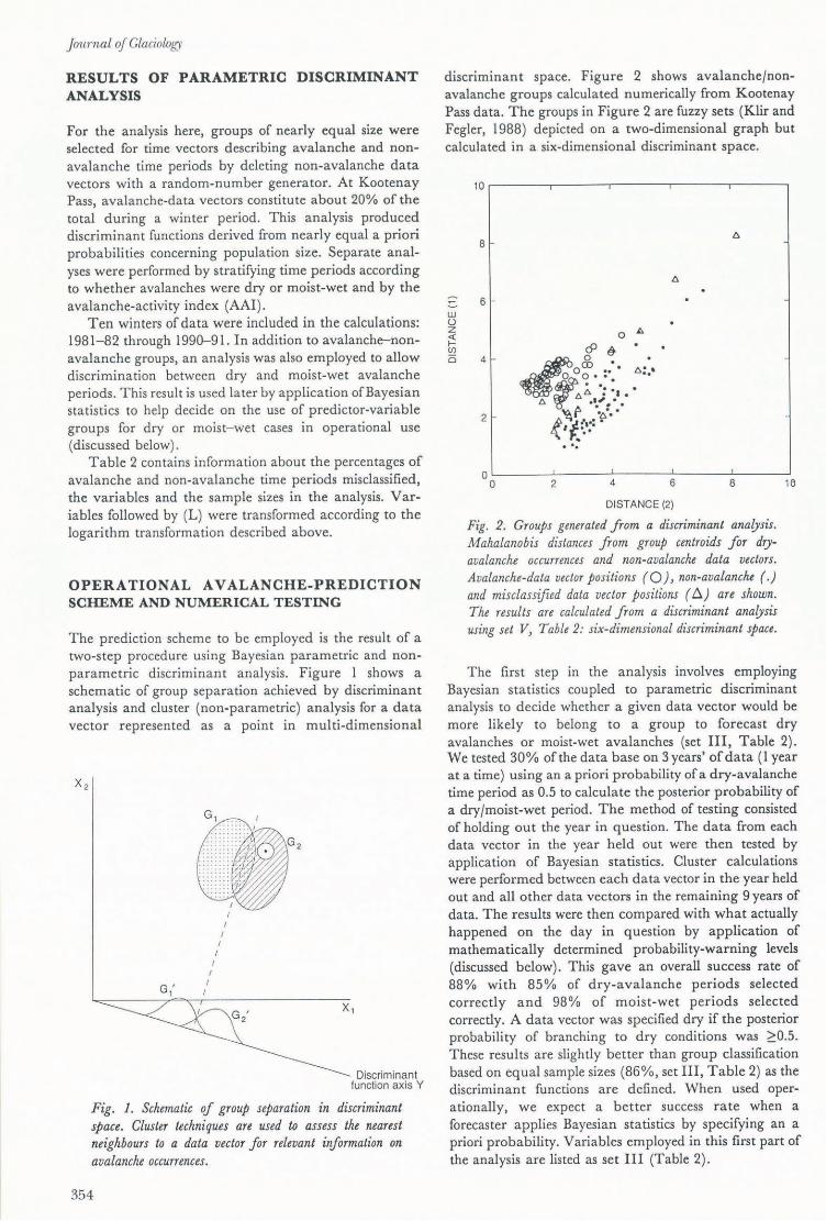
discriminant space. Figure 2 shows avalanche/non­avalanche groups calculated numerically from Kootenay Pass data. The groups in Figure 2 are fuzzy sets (Klir and Fegler, 1988) depicted on a two-dimensional graph but calculated in a six-dimensional discriminant space.

10~------~-----,-------,-------.------,

8

:::. 6 w u z ~ (f)

o 4

2

OL-____ ~ ______ -L ______ ~ ____ ~L-____ ~

o 2 4 6 8

DISTANCE (2)

Fig. 2. Groups generated from a discriminant analysis. M ahalanobis distances from group centroids for dry­avalanche occurrences and non-avalanche data vectors. Avalanche-data vector positions (0), non-avalanche (.) and misclassified data vector positions (6:.) are shown. The results are calculated from a discriminant analysis using set V, Table 2: six-dimensional discriminant space.

The first step in the analysis involves employing Bayesian statistics coupled to parametric discriminant analysis to decide whether a given data vector would be more likely to belong to a group to forecast dry avalanches or moist-wet avalanches (set Ill, Table 2). We tested 30% of the data base on 3 years' of data (1 year at a time) using an a priori probability of a dry-avalanche time period as 0.5 to calculate the posterior probability of a dry/moist-wet period. The method of testing consisted of holding out the year in question. The data from each data vector in the year held out were then tested by application of Bayesian statistics. Cluster calculations were performed between each data vector in the year held out and all other data vectors in the remaining 9 years of data. The results were then compared with what actually happened on the day in question by application of mathematically determined probability-warning levels (discussed below). This gave an overall success rate of 88% with 85% of dry-avalanche periods selected correctly and 98% of moist-wet periods selected correctly. A data vector was specified dry if the posterior probability of branching to dry conditions was ~O.5.

These results are slightly better than group classification based on equal sample sizes (86%, set Ill, Table 2) as the discriminant functions are defined. When used oper­ationally, we expect a better success rate when a forecaster applies Bayesian statistics by specifying an a priori probability. Variables employed in this first part of the analysis are listed as set III (Table 2).

The second step of analysis involves application of Bayesian statistics to determine the probability of avalanching. Either set I (dry avalanching) or set II (moist-wet avalanching) of variables are selected depend­ing on the results of the first step of the analysis.

We tested the results of steps one and two of the analysis by applying Bayesian statistics (a priori prob­ability = 0.5) to 3 years of the data set (1984-85, 1987-88 and 1990-91 ). A warning (avalanche prediction) was issued if the probability of dry avalanching was ~0.6 and if the probability of moist-wet avalanching was ~O. 7. These levels (0.6 and 0.7) were determined mathematic-

~ :J m <{ en o a: a. w I o Z ::; « > «

~ :J m « en o a: a. w I o z « ..J « > «

0.8

0.6

0.4

0.2

0.00L-------1-'-0-0--"'-----2.L

00---------:-'·300

TIME PERIOD

Fig. 3. Avalanche probability for 1984-85 calculatedJrom discriminant-analysis predictions (.) vs avalanche occur­rences (0). For the avalanche occurrences, if no circle (0) appears, no avalanches were recorded. Both dry and moist-wet avalanches are shown. Warning level is 0.6 Jor dry avalanches, 0.7 Jor moist-wet avalanches. Variable sets J and 11 (Table 2) were used in the calculations.

0.8

0.6 I

1 I 11

, ~

0.4 1

0.2

:-I II

0.0 L-_____ --'-______ -'--_____ _ ---'

o 100 200 300

TIME PERI OD

Fig. 4. Similar to Figure 3for dataJrom 1987- 88.

McClung and Tweedy: Numerical avalanche prediction

ally to achieve an approximate equal balance between the percentage of avalanche and non-avalanche periods predicted correctly. The predicted results were then compared with what actually occurred (avalanching or not) during the time period. The results gave 79% success rate for dry-avalanche prediction (79% of non-avalanche periods; 78% of avalanche periods). For moist-wet avalanche periods, 75% success rate was achieved (75% non-avalanche periods, 71 % wet-moist avalanche per­iods). These results are comparable to sample classific­ation based on equal sizes during development of the discriminant functions (see Table 2) using equal sample sizes. Figures 3 and 4 show the results of our numerical testing for 2 years of observations.

CLUSTER ANALYSIS OF A DATA VECTOR

In addition to calculating the probability of occurrence of avalanching, we also use cluster analysis to provide a further description of "nearest neighbours" to the time vector (e.g. Obled and Good, 1980; Buser, 1983; Buser and others, 1987). Our method of determining nearest neighbours consists of calculating the Mahalanobis distance D2 between all vectors in the data Xi base and the current one: Xp

2 ( - -)' -1 ( - - ) Dip = Xi - Xp S Xi - Xp (9)

where Sl is the inverse of the pooled within-groups variance-covariance matrix calculated as a part of the discriminant analysis. This distance and variance­covariance matrices are calculated using the variables of either set I or set II in Table 2, depending on whether dry avalanching or moist-wet avalanching may be expected. This distance metric reduces to the Euclidean distance metric assumed by Buser and others (1987) if the variance-covariance matrix is taken to be the identity matrix. Therefore, our distance matrix retains the assumption that the variables are correlated and distances are calculated in discriminant space in contrast to the implicit assumption of no correlation between variables if a Euclidean metric is chosen.

On calculation of distances between data vectors, the distances are ranked and the 30 nearest neighbours are retained and analyzed for information as to whether they have avalanche occurrences associated with them, and information about the avalanches is summarized. This information includes: size, moisture (dry, moist, wet), trigger, aspect, location, type (slab or loose snow) and other parameters. The fraction of data vectors in the nearest-neighbour cluster which contain avalanching may be regarded as similar to a conditional probability of avalanching for the cluster analysis. We have studied two values of probability (PlO and P30), which describe the conditional probability of avalanching for the ten and 30 nearest neighbours to the present data vector. Our study had two objectives: (I) to determine whether the Bayesian discriminant probability or conditional cluster probabilities correlated best with avalanche activity; (2) to assess whether PlO and P30 correlated best with the Bayesian discriminant probability.

The answer to objective (I) was sought in two parts:

j oum al of Glaciolo!:,'Y

(a) by a simple correlation, e.g. Spearman Rank correlation, and (b) by comparing conditional probabil­ity of avalanching calculated by both methods. Both (a) and (b) showed that Bayesian discriminant probabilities were superior to conditional cluster probabilities in our study. Rank correlation between magnitude of avalanch­ing and Bayesian probabilities is shown in the correlation Table 3.

Table 3. Rank correlation matrix for AA!, P, PlO, P30 for data from 1985, 1988 and 1991

Matrix of Spearman correlation coefficients

AA! P PlO P30

AAI 1.000 P PlO P30

0.371 0.363 0.366

1.000 0.580 0.712

1.000 0.798 1.000

These data show that the Bayesian probabilities correlate best with the avalanche magnitude-frequency index but the differences are minor. In order to compare predictions from the cluster probabilities with Bayesian probabilities, it was necessary to establish a prediction level (warning level) for the cluster predictions. It was found mathematically that the optimal prediction level

Table 4. Groups (rows) by prediction (columns) for winters of 1985, 1988, 1991 combined

Prediction with P30:

Non-avalanche Avalanche

Non-avalanche

477 43

Avalanche

113 91

72% of periods successfully predicted.

Prediction of dry avalanches Non-avalanche Avalanche (discrimination analysis):

Non-avalanche 268 70 Avalanche 19 63

79% of periods successfully predicted when dry avalanches are most likely.

Prediction of moist-wet avalanches

(discriminant analysis) :

Non-a valanche Avalanche

~56

Non-avalanche Avalanche

233 12

79 29

74% of periods successfully predicted when moist­wet avalanches are most likely.

was obtained when P30 = 0.20; when 20% of the 30 nearest neighbours contained avalanche occurrences, the best balance between successful prediction of avalanche and non-avalanche periods was achieved. This "warning level" is comparable to the optimum warning levels of 0.6 for dry avalanches and 0.7 for moist-wet avalanches. Table 4 gives a summary of results for data from the winters of 1985, 1988 and 1991. The results are tabulated in numbers of data vectors.

I t is important to note that, for the results in Table 4, there were 12 dry avalanche periods found in periods which were predicted by use of discriminant probabilities to be more likely to produce dry-avalanche periods. When these are taken into account, the fraction of avalanche periods correctly predicted by the two methods is virtually identical but non-avalanche periods are best predicted by the Bayesian-discriminant probabilities (77%) vs (73%) by using cluster techniques . Our conclusion then is : for the analysis using Kootenay Pass data, application of Bayesian discriminant technique is superior but there is not much difference between the two methods. Since our operational forecasting procedures will use both methods, Bayesian statistics to predict avalanches and cluster techniques to analyze expected ch a racter of avalanche occurrences, the consistency between the two m ethods is both advantageous and necessary.

TIME-SERIES ANALYSIS

Our model contains temperature and snowfall variables (and perhaps others) which allow a memory effect in the prediction capabilities. To study the time relation between probabilities and the AAI (see Table 3), we calculated the cross-correlation time series on a year-by­year b asis for the numerical experiments given in Table 4. Figures 5 and 6 show the correlation coefficients for 1984-

I--Z w g LL LL W 0 U Z 0 f= <>:: ...J w er: er: 0 u

0.4 c-------,-------,-------,--- - ----,

0.3

0.2

0. 1

-0. 1

-0.2 L---___ ---"-____ ---"--____ --'--___ ------'

-10 -5 0 5 10

LAG (TI ME PERIODS)

Fig. 5. Time-series cross-correlation of avalanche occurrences (AA!) with probabili!J (P) as predicted for 1984-85 (see Fig. 3). The limits of ± 2 standard errors above ~ero are shown ( . - .) .

f--z W (5 u:: LL W 0 0 Z 0 i= :5 w a: a: 0 0

0.4

0.3

0 .2

0.1

0 .0

-0.1

-0.2 -10 -5 0 5

LAG (TIME PERIODS)

Fig. 6. Cross-correlation of 1984-85 avalanche occurrences (AAI) with probabiliry of avalanching (P30) calculated from 30 nearest neighbours in discriminant space. The limits of ± 2 standard errors above zero are shown (-). Variable sets I and II (Table 2) are usedfor the calculations.

85 calculated by cross-correlation of AAI and P (Fig. 5) and P30 (Fig. 6). Figures 5 and 6 also show the limits of ± 2 standard errors above zero correlation: when the correlation falls inside these ranges, it is not considered significant. The results shown indicate that correlation between avalanching and the probability from the model becomes significant about two time periods (1 d) prior to the present (zero lag) . In addition, the results in Figures 5 and 6 show that the correlation between avalanching and the probabilities approaches insignificance after about one time period past maximum correlation (zero lag).

SUMMARY AND DISCUSSION

We have modified some of the numerical procedures for dealing with the numerical part of the avalanche­forecasting problem. Our methods are derived from the suggestions of Obled and Good (1980), Buser and others (1987) and LaChapelle (1980). Our resulting model involves using both parametric discriminant-analysis techniques (incorporating Bayesian statistics) and cluster techniques and "nearest neighbours" calculated in discriminant space using the Mahalanobis distance as the distance metric.

LaChapelle (1980) first advocated the use of Bayesian statistics in avalanche forecasting in the manner in which we intend to employ it by field testing our model. It is our belief that by combining a forecaster's a priori probability with our numerical estimate of the conditional prob­ability of avalanching, we can assess the potential power of an expert system employing symbolic logic to non­numerical data of classes i and ii. We have been able to include some data from these classes (e.g. avalanche occurrences) but not enough to produce a forecasting tool of the accuracy desired in applications.

McClung and Tweedy: Numerical avalanche prediction

The consistency of the results presented in comparing the cluster analysis and parametric discriminant analysis prove that these techniques are nearly identical when calculations are done in discriminant space. Application of the cluster techniques (along with parametric discriminant analysis) allows an operational forecaster to analyze the character of expected avalanche occur­rences if any appear in the clusters. For example, triggering mechanism, avalanche type and terrain information, such as avalanche-path location and aspect of avalanche release. The consistency in our comparison of results adds confidence that the mathematical procedures are correct in both cases.

Even though we have not field-tested our model, we believe that our numerical testing of the model is among the most extensive reported for numerical forecasting models. When Bayesian statistics are actually employed by forecasters, we have good reason to believe that the predictive accuracy we have estimated numerically will be exceeded. Since groups calculated by discriminant techniques (e.g. Fig. 2) are fuzzy, a future goal for avalanche forecasting may be to provide estimates of a priori probabilities from application of fuzzy logic procedures coupled with symbolic computing.

ACKNOWLEDGEMENTS

We wish to thank Dr O . Buser, Swiss Federal Institute for Snow and Avalanche Research, for his encouragement and help with this research. This research was supported by the British Columbia Ministry of Transportation and Highways, the National Research Council of Canada and the Natural Sciences and Engineering Research Council of Canada. We are indebted to the staff of the Snow Avalanche Section of the British Columbia Ministry of Transportation and Highways for providing data-hand­ling and avalanche-forecasting expertise. We are also grateful for the vision of E . A. Lund, Chief Highway Engineer, British Columbia Ministry of Transportation and Highways, for making this study possible.

REFERENCES

Bois, P., C. Obled and W. Good. 1975. Multivariate data analysis as a tool for day-by-day avalanche forecast. InternatioMl Association of Hydrological Sciences Publication 114 (Symposium at Grindelwald 1974 - Snow Mechanics), 391-403.

Bovis, M.]. 1976. Statistical analysis. In Armstrong, R. L. and]. D. Ives, eds. Avalanche release and snow characteristics, San Juan Mountains, Colorado. Boulder, CO, University of Colorado. Institute of Arctic and Alpine Research, 83-130. (INSTAAR Occasional Paper No. 19.)

Bovis, M.]. 1977. Statistical forecasting of snow avalanches, San]uan Mountains, southern Colorado. J. Glaciol., 18(78), 87-99.

Buser, O. 1983. Avalanche forecast with the method of nearest neighbours: an interactive approach. Cold Reg. Sci. Technol., 8(2), 155--163.

Buser, O. and W. Good. 1985. Avalanche forecast: experience using nearest neighbours. International Snow Science Workshop Proceedings. October 2+-27, 1984, Aspen, Colorado, 109-115.

Buser, 0., M. Biltler and W. Good. 1987. Avalanche forecast by nearest neighbour method. International Association of Hydrological Sciences Publication 162 (Symposium at Davos 1986-Avalanche Formation, Movement and Effects), 557-569.

357

Journal of Glaciology

Eisenbeis, R. A. and R. B. Avery. 1972. Discriminant analYsis and classification procedures. Lexington, MA, Lexington Book.

Ferguson, S. A., M. B. Moore, R . T. Marriott and P. Speers-Hayes. 1990. Avalanche weather forecasting at the Northwest Avalanche Center, Seattle, Washington, U.S.A. J. Glaciol., 36(122), 57-.Q6.

Klir, G.J. and T. A. Fegler. 1988. Fua:;; sets, uncertainlY and iriformation. Engelwood Cliffs, NJ, Prentice Hall.

LaChapelle, E. R. 1980. The fundamental processes in conventional avalanche forecasting. J. Glaciol., 26 (94), 75-84.

McClung, D. M. and P. Schaerer. 1993. TM avalancM handbook. Seattle, WA, The Mountaineers.

McClung, D. M. and J. Tweedy. 1993. Characteristics of avalanching:

Kootenay Pass, British Columbia, Canada. J. Glaciol., 39(132), 316-322.

Obled, C. and W. Good. 1980. Recent developments of avalanche forecasting by discriminant analysis techniques: a methodological review and some applications to the Parsenn area (Davos, Switzer­land) . J. Glaciol., 25 (92), 315-346.

Tatsuoka, M. M . 1971. Multivariate analYsis: techniques for educational and psychological research. New York, John Wiley and Sons.

The accuracy of the the references in the text and in this list is the responsibility of the authors, to whom queries should be addressed.

MS received 8 September 1992 and in revised form 1 April 1993

358