AFFDL-TR-e9-67

CO

O A NON-GAUSSIAN TURBULENCE SIMUUTION

& PAUL M. REEVES

TECHNICAL REPORT AFFDL-TR-e9-ö7

NOVEMBER 1969

'!&£&

This document has been approved for public release and sale; its distribution is unlimited.

AIR FORCE FLIGHT DYNAMICS LABORATORY AIR FORCE SYSTEMS COMMAND

WRIGHT-PATTERSON AIR FORCE BASE, OHIO

NOTICE

When Government drawings, specifications, or other data are used for any purpose

other than in connection with a definitely related Government procurement operation,

the United States Government thereby incurs no responsibility nor any obligation

whatsoever; and the fact that the government may have formulated, furnished, or in

any way supplied the said drawings, specifications, or other data, is not to be regarded

by Implication or otherwise as in any manner licensing the holder or any other person

or corporation, or conveying any rights or permission to manufacture, use, or sell any

patented invention that may in any way be related thereto.

fin. HMl <««/• v&b.\

M

Copies of this report should not be returned unless return is required by security

considerations, contractual obligations, or notice on a specific document.

500 - January 1970 - C04SS - 106-2343

A NON-GAUSSIAN TURBULENCE SIMULATION

PAVL M. REEVES

This document has been approved for public release and sale; its distribution is unlimited.

FOREWORD

This report was prepared for the Air Force Flight Dynamics Laboratory by the University of Washington. The study was conducted under United States Air Force Contract No. F 33615-67-C- 1851, "Analytical Investigation of Turbulence Models for Use in V/STOL Flight Simulators". The work was administered by the Air Force Flight Dynamics Laboratory; Mr. Evard Flinn was the Technical Monitor.

The work was supervised by the Principal Investigators, Professors R. G. Joppa and V. M. Ganzer of the Department of Aeronautics. The report was prepared by Paul M. Reeves.

The reporting period was October 1967, to May 1969. The report was submitted in June of 1969.

The author would like to thank Professors Joppa and Ganzer for their assistance and encouragement in carrying out the work. He also thanks the staff of the Department of Aeronautics for their assistance in preparing the report, particularly Carolyn •Taylor who typed both the original and revised manuscripts. Finally, the author gratefully acknowledges the assistance of Mr. Piinn throughout the work.

This technical report has been reviewed and is approved.

^SLüh^^äS^. C. B. Westbrook Chief, Control Criteria Branch Flight Control Division Air Force Flight Dynamics Laboratory

ii

ABSTRACT

A comparison of the statistical properties of low altitude atmospheric turbulence and the characteristics of presently used simulation techniques shows that these techniques do not satis- factorily account for the non-Gaussian nature of turbulence. A non-Gaussian turbulence simulation, intended to be used in con- junction with piloted flight simulators, is developed.

The simulation produces three sisvaltaneous random processes which represent the three orthogonal gust components. The proba- bility distribution of each component is characterized by the modified Bessel function of the second kind of order ?ero, K0 t and the power spectral densities suggested by H. L. Dryden are used in a slightly modified form. The rms intensity and scale length of each component are independent parameters. A general method of introducing cross spectra between components is demon- strated.

The multiplication of independent random processes is used to generate each of the gust components. Gaussian white noise generators, analog multipliers, and linear filters are used throughout the simulation. A complete analog circuit diagram is presented.

111

TABLE OF CONTENTS

SECTION PAGE

I. INTRODUCTION 1

II. STATISTICAL CHARACTERISTICS CF LOW ALTITUDE ATMOSPHERIC 2 TURBULENCE

A. Homogenei i.y 2 B. Stationarity 3 C. Erobability Density Distribution 3 D. RMS Intensity 7 E. Normalized Power Spectral Densities 8 F. Correlation Tensor and Cross Spectra 12 G. Summary of Turbulence Characteristics 12

III. PRESENT TURBULENCE SIMULATIONS 14

A. Filtered White Noise Turbulence Simulation 14 B. Recorded Time History Turbulence Simulation 14 C. Sum of Since waves Turbulence Simulation 15 D. Summary 15

IV. FORMULATION OF A NON-GAUSSIAN TURBULENCE SIMULATION 16

A. General Approach 16 B. Some General Statistical Relationships 18 C. Simulation of the Three Gust Components 18

1. Probability Density 18 2. Generation of the Vertical Gust Spectrum 20 3. Generation of the Longitudinal Gust Spectrum 22 4. Generation of the Lateral Gust Spectrum 26

D. Generation of the w - u Cospectrum 29

V. REVIEW AND DISCUSSION OF DEVELOPMENT 37

A. Review of Development 37 B, Discussion of Simulation 41

1. Simplicity 41 2. Simulation of the "Patchy" Turbulence Structure 41 3. Ideal Circuit Elements 47 4. Extension to Spatial Distribution 48 5. Restrictions on Vehicle Flight Path 48

VI. SUMMARY 49

REFERENCES 50

APPENDIX: Derivation of General Statistical Relationships 54

iv

ILLUSTRATIONS

FIGURE PAGE

1. Typj-wcjjL Probability Densities 4

2. Comparison of Gaussian and K0 Probability Densities 6

3. Normalized Power Spectral Densities 11

4. Vertical Gust Analog Circuit 23

t;. Longitudinal Gust Analog Circuit 27

6. Lateral Gust Analog Circuit 28

7. Cross Correlation Fil^3r Array 30

8. Cospectral Density 35

9. Final Analog Circuit 42

SYMBOLS

a Ranöoin function of time

A Constant

b Random function of time

B Constant

C Correlation function (See list of definitions)

D Constant

f Frequency (cps)

h Impulse response function

H Transfer function (the Laplace transform of h)

i Imaginary, /Ti

K Constant

L Scale length of turbulence (ft)

m Random function of time

n Random function cf time

p Random function of time

P Probability density function

3P Probability distribution function

q Random function of time

r Random function of time

s Laplace transform variable

t Time (sec)

T Time (sec)

u Longitudinal gust component - aligned with mean wind positive in the direction of the mean wind (ft/sec)

Ü Mean wind speed (ft/sec)

vi

SYMBOLS (Cont'd.)

v Lateral gust component - forms right handed system with longitudinal and vertical gust components (ft/sec)

w Vertical gust component (ft/sec)

x Dumny variable

y Dummy variable

z Dvnrnny variable

a Dummy variable

ß Dummy variable

Y Dummy variable

6 Dyrac delta function (See list of definitions)

T] Gaussian white noise signal with zero mean value

K0 Modified Bessel function of the second kind of order zero (See list of definitions)

a rms intensity (See list of definitions)

T Correlation variable (sec)

f Cross spectrum (See list of definitions)

f Power spectrum (See list of definitions) pp

♦ Cospectrum (See list of definitions)

$ Normalized power spectrum (See list of definitions) pq

VP

Operators

E[] Expected value (See list of definitions)

* Convolution (See list of definitions)

VI i

SYMBOLS (Cont'd.)

Subscripts

t Function of t

T Function of T

Superscript

* Complex conjugate

Analog Symbols

D O

Summer

Integrator

Multiplier

Potentiometer

va 11

DEFINITIONS

The following functions appear repeatedly throughout the following report. Their mathematical definitions are collected here for convenient reference.

A, Convolution

p(t) * q(t) = f p(T}q(t - T)dT (DEF-1)

B. Correlation

The general correlation tensor is defined by the relationship

Cpq(x' &x' y» W' z' Az' t' T) =

(DEF-2)

<p{x, y, z, t)q(x + Ax, y -f- Ay, z + Az, t + T)^

where ^ } denotes ensemble average.

If the processes p and q are stationary, C can be written ^

Cpq(x' Ax' y' Ay' z' &z' T) =

(DEF-3)

T

T^» 2T $ P(X' y' Z' t)q(X + "X' y + Ayj Z + Aa' t + T)dt -T

In this report spatial separation (Ax, ly, Az) will not be considered, and turbulence will be ass.uned homogeneous in the x - y plane. Therefore Cpq will not be a function of x. Ax, y, Ay, or Az. Dependence upon height z will be expressed as a depondence upon scale length L. Finally, the formal listing of the argument L will be suppressed.

IX

DEFINITIONS (Cont'd.)

The cross correlation of p and q is then defined

T Cpq(T) =T^2T I P{t>a-lt + T>dt {D£F-4)

vhere Cpq(T) is understood to possibly be a function of scale length L .

If p and q are identical, (DEF-4) becomes the auto- correlation, C (T) . pp

(DEF-5)

Implementing the expected value notation of (OEF-8)

Cpq(T) = EfP(t,q(t + T)1 (DEF-6)

In terms of the power spectral density

cpp(i) = L*K>(f,ei2TTfTdf (DEF"7)

C. Expected Value

«»«^ - £!i^PU)« (DEF.0)

DEFINITIONS (Cont'd.)

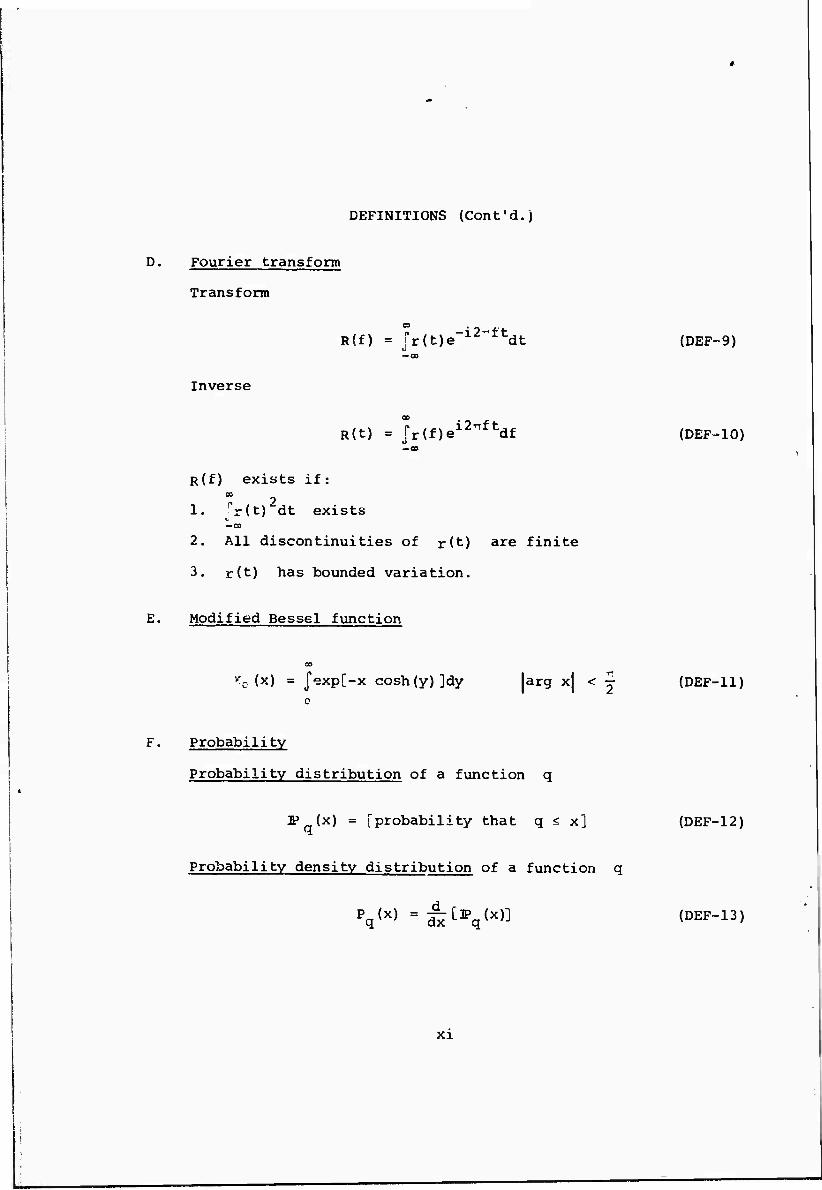
D. Fourier transform

Transform

R(f) = fr(t)e"i2"ttdt (DEF-9)

Inverse

R(t) = ]:r(f)ei2,Tftdf (DEF-10)

R(f) exists if:

1. "rU) dt exists — 00

2. All discontinuities of r(t) are finite

3. .r(t) has bounded variation.

Modified Bessel^function

•'o (x) = Jexp[-x cosh(y)]dy |arg x| < ^ (DEF-ll)

F. Probability

Probability distribution of a function q

IP (x) = [probability that q s x]

Probability density distribution of a function q

(DEF-12)

Pq(x) =ÄtlPq(x)] (DEF-13)

XI

DEFINITIONS (Cont'd.)

G. RMS intensity

rms of a function p(t)

^-":V^ITp(t)2at (DEF-l4,

H. Spectra

The cross spectrxom of two functions p(t) and q(t)

QD

Wf) = r Cna(T)e"i2"fTdT (DEF-15)

The cospectruin of p(t) and q(t) is the real part of $ (f)

1 (f) = Re{$ {f)l (DEF-16) pq W

That is, $ (f) is obtained by Fourier transforming the cpq

correlation tensor.

The power spectral density or power spectrum of p(t)

00

fPP(f) = •jraoCPP(')e"i2^fTd'r (DEF-17)

1 (f) fn (f) = PP2 (DEF-18)

PP ap

*

xii

SECTION 1

INTRODUCTION

The development of a new aircraft, particularly one of the V/STOL variety, is greatly facilitated by a piloted simulation of the vehicle. A simulator permits pilot evaluation of handling qualities, operating procedures, and other important factors before the vehicle itself has been constructed. Of course the simulation must be as realistic as possible if the results are to be trustworthy.

Atmospheric turbulence is a particularly important effect in low altitude operation. Consequently, a random external distur- bance which simulates atmospheric turbulence is frequently used in low altitude simulations to present the pilot with a more realistic control task. Though the benefits to be derived from a realistic simulation are worthy of considerable effort, little attention has been given to the realistic simulation of turbulence.

The object of this report is to review the characteristics of low altitude atmospheric turbulence, compare the characteristics of presently used turbulence simulations to those of real turbu- lence, and finally to suggest a simulation which is more realistic than those presently used.

The following development is divided into four parts. Section II considers the characteristics of real turbulence and the impor- tance of those characteristics to simulator realism. The proba- bility distribution, rms intensity, power spectral and cross spec- tral densities are discussed and suggestions for analytical forms to be used in simulation are made.

Section III presents a summary of presently used turbulence simulation techniques. These are discussed in view of the char- acteristics of real turbulence described in Section II.

Section IV formulates an analog circuit which produces a non- Gaussian turbulence simulation. A complete mathematical develop- ment is presented, beginning with the derivation of necessary sta- tistical relationships. The result is an analog circuit which pro- duces outputs statistically similar to the three components of atmospheric turbulence occurring at a point in space. Conventional analog equipment and ordinary Gaussian white noise generators are used throughout.

Section V summarizes the results of Section IV for those read- ers who wish to omit the mathematical development, and discusses the simulation in some detail. Complete analog circuit diagrams are presented.

SECTION II

STATISTICAL CHARACTERISTICS OF LOW ALTITUDE ATMOSPHERIC TURBULENCE

Obviously the characteristics of real turbulence must be known before a turbulence simulation can be specified. Unfortunately, the mechanism of turbulence and the effects of changing atmospheric conditions upon its structure are not understood now and will prob- ably remain so for some time. Any description of turbulence is therefore restricted to a discussion of its experimentally deter- mined statistical properties.

This section will not attempt to review the tremendous amount of data which has been published on the subject of atmospheric turbulence. Instead, some typical statistical properties of turbu- lence will be considered in view of the problem of realistic simulation. Only neutral stability conditions will be investigated since the greatest problems in vehicle control, and therefore the greatest need for a realistic simulation, result from high wind conditions.

This section is divided into seven prrts and considers the homogeneity, stationarity, probability density, rms intensity, power spectra, and cross spectra of atmospheric turbulence. The final section summarizes these points.

A. Homogeneity

To say that atmospheric turbulence is homogeneous implies that its statistical properties are not functions of the spatial coor- dinates. Unfortunately low-altitude turbulence does not demon- strate this property.

Chapter 5 of Reference 1 presents data showing that the scale length of the vertical gust component varies proportionally to altitude. This effect will be discussed more completely in part D below. Reference 2 reports that the terrain underlying &. turbu- lent region can strongly affect its intensity. Thus the tiv bulence encountered by a vehicle can be expected to vary as the vehicle moves over different surface features. A similar effect, the "patchy" structure of turbulence which will be discussed at length in Part C below, implies that a variation of intensity with spatial location is an intrinsic characteristic of turbulence.

Of these inhomogeneous effects, only those due to altitude variation and the "patchy" structure appear to be intrinsic to turbulence and therefore necessary features of a realistic simula- tion. Though the influence of terrain may be required for the simulation of certain flight tasks

(see for example Reference 3), it will not be considered here as a typical feature of turbulence.

B. Stationarity

Atmospheric turbulence is a stationary process if its statis- tical properties are independent of time. This is, of course, not true if very long time periods are considered because changing large-scale meteorological conditions are likely to introduce changes in the turbulence structure and intensity. However, few simulations operate continuously over such a lengthy period. Most require only a few minutes of operation, during which the turbulence can be assumed stationary. Therefore nonstationary effects need not be considered in a typical simulator application.

C. Probability Density Distribution

The probability density distribution of a random process, more commonly called its probability density, is a measure of the likelihood that any particular state will occur. For example, the probability density of the vertical gust component describes the likelihood that a vertical gust velocity of any particular magni- tude will occur. A mathematical definition is given in the list of definitions. Note that the continuous velocity time history is to be considered, not merely peak gust velocities.

Despite considerable amounts of data describing gust exceedence probability based on total flight time (see for example References 4 and 5), there is little data on the probability distribution of gust velocities in continuous turbulence. A Gaussian distribution has been widely assumed in the past because some data did seem to indicate a normal distribution and because of the great statistical simplifications which result. Unfortunately there is mounting evi- dence that turbulence is not a Gaussian process.

Reference 6, for example, presents a computer analysis of measurements taken by a hot wire anemometer in a wind tunnel. The results indicate that grid generated turbulence is non-Gaussian.

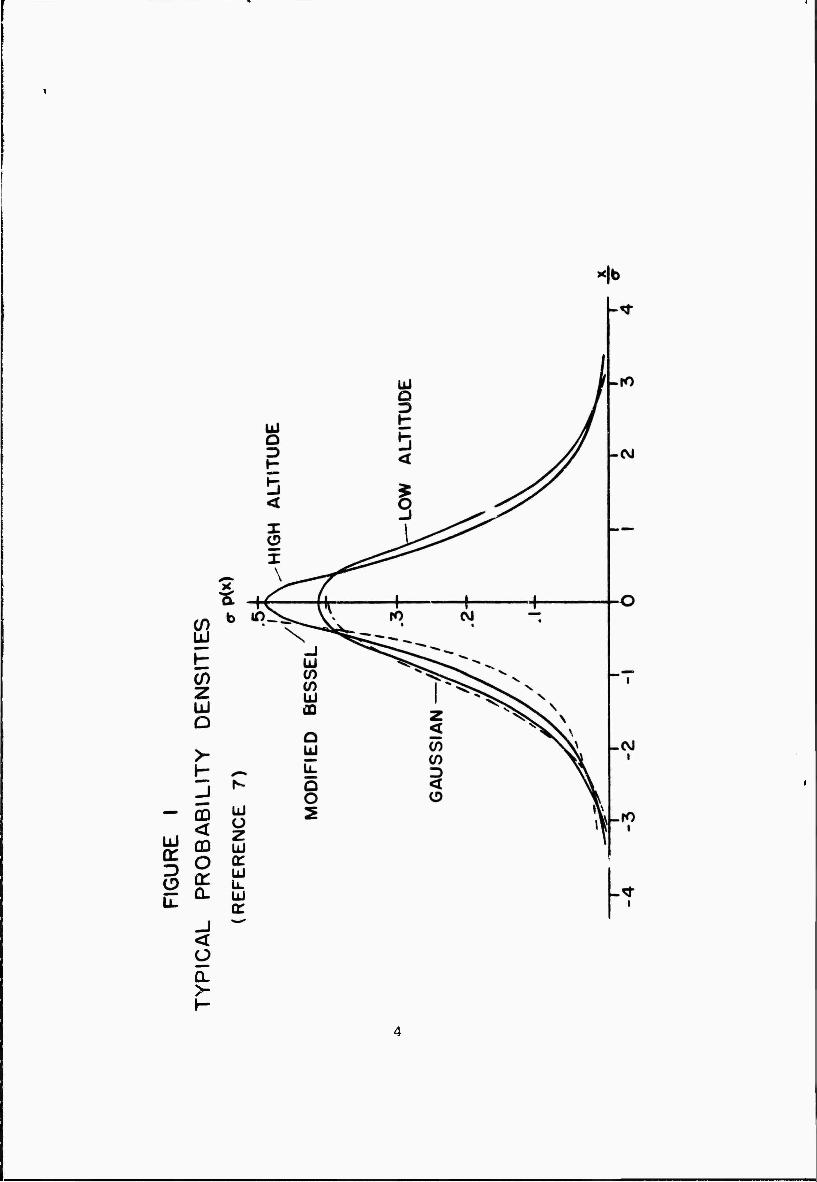
Reference 7 contains an analysis of all three gust components at both high and low altitude showing that atmospheric turbulence is definitely non-Gaussian. The results indicate that low-altitude turbulence is more nearly Gaussian than that at high altitudes, but at all altitudes the probability density exceeds that of a Gaussian distribution for both small and large absolute values of gust veloc- ity. Figure 1 indicates a typical result.

A study of peak accelerations reported in Reference 8 leads to

Q.

conclusions similar to those of Reference 7. Based upon a large number of four and one-half minute samples of acceleration data recorded during flight below 5,000 feet, the report finds that atmospheric turbulence is characterized by an exponential proba- bility density distribution of peak gust velocities. This leads to a gust velocity probability density characterized by the modi- fied Bessel function of the second kind of order zero, K0 .

P(X) = ~K0Ö ("-I)

This function is tabulated in many publications (see for example Reference 9). An integral representation will be found in the list of definitions. Figure 2 compares the Gaussian and K0 distribu- tions. Note that the modified Bessel function exceeds the normal curve at both large and small gust velocities.

The discontinuity of K0 when its argument becomes zero presents some difficulty. An experimental verification of this feature would require an infinitely long turbulence time history, or an infinite number of ensemble records. Such an analysis is, of course, impossible.

There is, however, an argument based upon the "patchy" nature of turbulence which leads to the choice of K0 to characterize its probability density. Turbulence apparently has a patchy struc- ture. That is, regions of intense turbulence are surrounded by areas of relatively calm air. Evidence for this structure is pro- vided by References 8, 10, 11, and 12. References 8 and 10 ref«ir specifically to low-altitude atmospheric turbulence. If one assumes that the turbulence within each patch is Gaussian and that the intensity of the turbulence varies from patch to patch in a continuous Gaussian manner, then the turbulence time history encountered by an aircraft flying through the region is actually the product of two independent Gaussian random processes. Part C of Section IV of this report demonstrates that the probability density of such a time history is characterized by the modified Bessel function K0 .

If a patchy structure is assumed, the more nearly Gaussian nature of low-altitude turbulence reported in Reference 7 can be attributed to the influence of surface roughness in producing a more homogeneous turbulent field. In this case longer samples might produce a more non-Gaussian result. It should be noted that the low-altitude data presented in Reference 7 have been filtered to remove wavelengths longer than 7,000 feet.

The "patchy" structure of turbulence thus suggests a modified Bessel function probability density as shown in Figure 2. This distribution will be adopted as descriptive of atmospheric turbu- lence.

4 4

Q.

b

2H

i A

FIGURE 2

COMPARISON OF

PROBABILITY DENSITIES

GAUSSIAN

MODIFIED BESSEL FUNCTION

T 2 3

a

The above arguments are independent of gust direction, there- fore the ic0 distribution should be appled to all three gust com- ponents. Ideally there should be some definition of patch size as a function of altitude, but these data are presently unavailable. The assumed probability densities are expressed in Equations (II-2), (11-3), and (II-4) below.

u u

PV(X)=J-M^) (ii-3)

pv(l"^«<' (I1-4'

D. RMS Intensity

The rms, or variance, of a random disturbance is a measure of its intensity. A mathematical definition of this quantity is given in the list of definitions.

Reference 1 indicates that the intensity of turbulence at low altitude in neutral conditions is influenced by both the mean wind speed and the surface roughness, in general therefore, the absolute intensity chosen for a particular simulation must depend upon the environment being simulated.

The ratios of the individual gust component rms values have been measured by several investigators. Typical results are:

(ju/av/ow = 2.5/2.0/1.05 (Reference 1) (II-5)

= 2.8/2.0/1.3 (Reference 13) (II-6)

= 1.0/1.16/.75 (Reference 14) (II-7)

There is apparently not much agreement on these ratios. Chapter 4 of Reference 1 contains a complete discussion of the problem.

The question of rms ratios is further complicated by human sensitivity. Reference 15 reports the results of an airborne simulation which indicates that pilots are strongly influenced in their handling qualities judgement by the rms of an external dis- turbance, it is therefore necessary that truly representative values be chosen for use in such research.

In view of pilot sensitivity and the spread of available data, it seems best to allow a free choice of the rms value of each gust velocity component.

E. Normalized Power Spectral Densities

It is best to begin this part with a clarification of the term power spectral density as used in this report. Many writers use what might be called a "one-sided" power spectral density, a func- tion of only positive frequencies. in this report a "two-sided" power spectral density, an even function of frequency, is assumed in order to ease the mathematical manipulations which follow. A description of the power spectral density is to be found in the list of definitions.

The normalized power spectral density can now be delined as the power spectral density divided by the mean square of the process. Thus the integral over frequency from minus to plus infinity is equal to unity. In the remainder of this report the term power spectral density will be shortened to spectrum or power spectrum.

Experience has shown that atmospheric turbulence has reason- ably consistent normalized spectra, but there is a considerable spread in the data. Many mathematical forms have been advanced, each supported by some experimental evidence, to describe these spectra. In particular, Reference 16 suggests the following normd-- Ized expressions for isotropic turbulence.

,n (f) = k __ 2 _ {II_8)

[1 + (1.339^p) ]5/6

2 T [1 + |(i.339^) ]

$ (f) = h 3 y^ (li_g)

U U + (la339^M) I11/6

T [1 + f(1.339^) ] in (f) =--§ ~ (11-10)

^ [I + (1.339^) )11/6

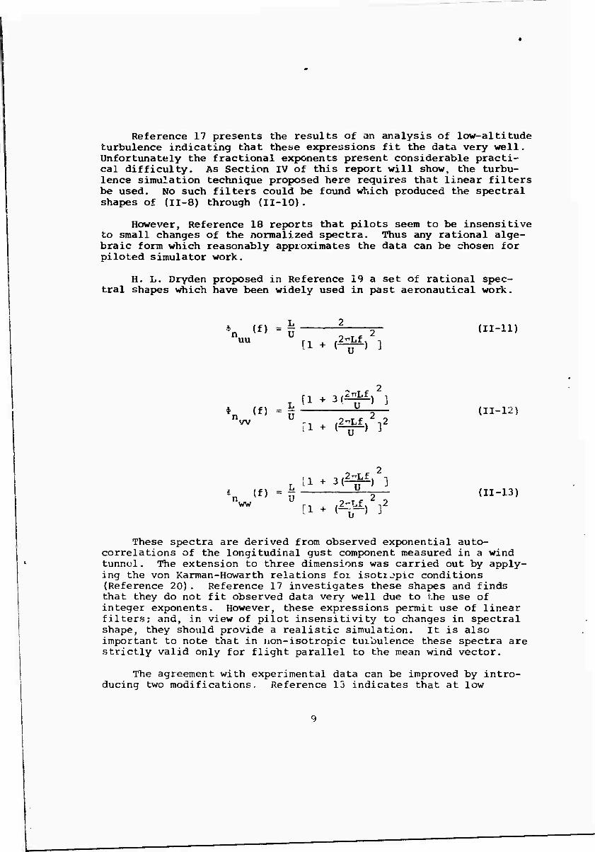
Reference 17 presents the results of an analysis of low-altitude turbulence indicating that these expressions fit the data very well, unfortunately the fractional exponents present considerable practi- cal difficulty. As Section IV of this report will show, the turbu- lence simulation technique proposed here requires that linear filters be used. No such filters could be found which produced the spectral shapes of (II-8) through (11-10).

However, Reference 18 reports that pilots seem to be insensitive to small changes of the normalized spectra. Thus any rational alge- braic form which reasonably approximates the data can be chosen for piloted simulator work.

H. L. Dryden proposed in Reference 19 a set of rational spec- tral shapes which have been widely used in past aeronautical work.

*n <f> = h r—ir tn-ii) ri + {ift) ]

2 T fl + 3(^) ]

fn (f) = U 2— (II-12)

VV 11 + (^) ]2

. [1 + 3(^)2] enww(f) =" 777^7 (II'13)

ww [1 + (^) ]2

These spectra are derived from observed exponential auto- correlations of the longitudinal gust component measured in a wind tunnul. The extension to three dimensions was carried out by apply- ing the von Karman-Howarth relations for isotupic conditions (Reference 20). Reference 17 investigates these shapes and finds that they do not fit observed data very well due to the use of integer exponents. However, these expressions permit use of linear filters; and, in view of pilot insensitivity to changes in spectral shape, they should provide a realistic simulation. It is also important to note that in non-isotropic turbulence these spectra are strictly valid only for flight parallel to the mean wind vector.

The agreement with experimental data can be improved by intro- ducing two modifications. Reference 13 indicates that at low

altitude the normalized spectrum of the lateral gust component matches the longitudinal spectrum much more closely than it matches the vertical spectrum. An obvious change is therefore a substitu- tion of the longitudinal spectrum (11-11) in place of the right-hand side of (11-12). The discussion in Part F below will indicate that the lateral gust component is independent of (i.e., uncorrelated with) the other two components. Therefore the lateral component can be modified without interfering with other parts of the simulation.

Another problem with the Dryden spectra is that the scale length L is the same in all three expressions. This does not seem to be verified by experimental evidence. Chapter 5 of Refer- ence 1 presents data indicating that the scale length of the verti- cal gust component varies proportionally to altitude above the surface. Reference 21, on the other hand, finds that the scale length of the longitudinal component is proportional to the 4/5 power of height. Therefore the two lengths cannot be equal at all altitudes. The results of Reference 13 also seem to indicate a difference in scale lengths, in view of this uncertainty it seems wise to allow the scale length of each gust component to vary independen tly.

When these changes are made, the normalized spectra become:

n. (f) =~ uu

L u U

2rrL f

[1 + (-^-) ] U

(11-14)

*n <f > = if w 2TrL f

[1 + (--—-) ] Ü

(11-15)

* (f) "ww

2TTL f Lw [1 + 3(-ir-> ] U 2nL f 2 .

w [i + (" U ) r

(11-16)

These expressions will be assumed to represent the normalized spectral densities of low-altitude atmospheric turbulence adequately. Equations (11-14), (IT-15), and (11-16) are plotted in Figure 3 in a form permitting direct comparison with most meteorological data.

10

11

F. Correlation Tensor and Cross Spectra

Having discussed the characteristics of individual gust co?nsv^ nents, it is now necessary to consider the relationship between components. This relationship is expressed in its most general form as the correlation tensor, complete discussions of which can be found in Relerences 1 or 22. This tensor expresses the correlation of gust time histories measured at different points in space and thus de- scribes the three-dimensional distribution of turbulence. If the correlation tensor is known, then such effects as rolling due to the distribution of vertical gusts along the wing span can be inclu- ded in a simulation of flight through turbulent air. U fortunately, very little is known about the form of the tensor in non-isotropic turbulence. Its full evaluation will require a tremendous amount of work, almost none of which has been carried out. There is very little information on spatial distribution in other than the down- wind direction. More data, particularly dealing with the lateral distribution, must be collected before spatial distribution effects can be included in a turbulence simulation.

If there is no spatial separation between the points at which gust velocities are to be correlated, the situation is somewhat simplified. Even in this special case, however, few pieces of data are available. Reference 13 presents the cospectral density rela- tions of the three gust components measured at various heights for a range of stability conditions. The relationship between the correlation tensor and the cospectral density is described in the list of definitions. The results indicate that only the vertical and longitudinal gusts have a significant cospectrum, that it is negative, and that it is non-zero only at low frequencies. The data spread is quite broad and no quadrature spectra are presented, therefore there is little reason to attempt an accurate algebraic representation. However, some correlation should be introduced since a general form is known.

obviously more information is required in this area before a realistic simulation of turbulence can be formulated. In this paper it will be assumed that a low-frequency correlation exists between the longitudinal and vertical gust components. No attempt to simulate the spatial distribution of turbulence will be made; that is, only the three gust components occurring at a single point will be modeled.

G. Summary of Turbulence Characteristics

The statistical characteristics of low-altitude turbulence which are important to simulator realism are summarized below.

(1) Stationarity

Low-altitude turbulence can be approximated by a station- ary process for most simulations. Long operating times,

12

on the order of several hours, require some allowance for changing weather conditions.

(2) Homogeneity

Turbulence seems to be intrinsically inhomogeneous. A simulation should include the effects of altitude vari- ation and the "patchy" structure of turbulence. Terrain features may have an influence in some instances, but this effect will not be considered here.

(3) Probability Density

Turbulence seems to be characterized by a modified Bessel function probability density as written in Equations (II-2), (II-3), and (II-4).

(4) RMS Intensity

The absolute rms intensity of turbulence is determined by prevailing conditions, and therefore no particular values can be specified. The rms ratios of the gust components are presently not well determined. A simula- tion should therefore allow the rms value of each gust component to be varied independently.

(5) Normalized Power Spectra

The gust components can be characterized by the normalized power spectra of Equations (11-14), (11-15), and (11-16). These forms do not fit experimental data particularly well, but they do permit the use of linear filters and should be sufficiently reaxistic for piloted simulations.

(6) Correlation Tensor and Cospectra

Very little is known about the spatial distribution of turbulence and the relationship between gust components. A negative cospectrum of the longitudinal and vertical gust components measured at the same point in space is indicated, but there are insufficient data to suggest an analytical form.

13

SECTION III

PRESENT TÜFBÜLENCE SIMULATIONS

This section briefly discusses the most common turbulence sim- ulation methods and compares their usefulness. Three basically different techniques have been found: the filtered white noise sim- ulation, the recorded time history simulation, and the sum of sine waves simulation. Parts A through C below discuss each of these methods in turn. Part D summarizes the results of this section.

A. Filtered White Noise Turbulence Simulation

This technique is by far the most common method of turbulence simulation (see for example Reference 15 and References 22 through 28). Time histories are generated by linearly filtering Gaussian white noise and amplifying the resultant signal so that the normal- ized spectrum and rms intensity match those of real turbulence-

This method requires few pieces of equipment and is very versa- tile. Reference 22, for example, proposes a filtered white noise turbulence simulation which allows for even the spatial dependeuce of the covariance tensor. In fact, the normalized spectra, rms intensities, cross spectra, and even (with some difficulty) the effects of inhomogeneity and spatial distribution can all be simu- lated using filtered white noise, unfortunately, the time histories produced have a Gaussian probability density. As discussed in Section II of this report, turbulence is not a Gaussian process. Therefore, although the filtered white noise method has many advan- tages, it must be considered an incomplete simulation because it does not reproduce the non-Gaussian nature of turbulence.

B. Recorded Time History Turbulence Simulation

This simulation of turbulence uses time histories of gjst velocities recorded during actual flight (see for example References 24 and 29). There can be little argument concerning the realism of such a technique. However, no allowance can be made for changes of altitude or different atmospheric conditions without the collec- tion of a very large nurober of time histories. Also, extended run- ning times cannot be accommodated without repetition. Therefore, while this model is certainly useful in the simulation of special conditions for which little or no statistical data is available, it does not appear to be flexible enough to provide a general turbulence simulation.

14

C. Sum of Sine Waves Turbulence Simulation

Reference 30 reports the use of a turbulence simulation pro- duced by summing the outputs of ten sine wave generators. This method seems to offer no advantage over the filtered white noise simulation discussed in Part A above unless some specific phase relationships between frequency components can be determined or unless the specific frequency content of the disturbance is an important factor in each test. At the present time there is no indication of fixed phase relationships in random turbulence, and most simulations do not require such complete knowledge of the frequency content. Therefore, this method appears to be inferior to the filtered white noise technique which produces an infinite number of frequency components.

D. Summary

The most versatile and widely used turbulence simulation is the filtered white noise method described in Part A above. It provides more flexibility than the recorded time history technique and contains more frequency components than the sum of sine waves technique. Virtually all of the statistical properties of turbu- lence with the exception of its non-Gaussian probability distribu- tion can be simulated.

In view of the flexibility offered by the filtered white noise technique, the next logical step toward the formulation of a real- istic turbulence simulation appears to be an extension of this technique to include a non-Gaussian probability distribution.

15

SECTION IV

FORMULATION OF A NON-GAUSSIAN TURBULENCE SIMULATION

The desired characteristics of the simulation can be summa- rized in the following points:

1. An analog network is to produce three simultaneous random processes. These three processes are to represent the three orthogonal gust components occurring at a point (such as the center of gravity of a vehicle).

2. Each component should have a probability density charac- terized by the modified Bessel function of the second type of order zero, K0 .

3. The simulated gust time histories are to have the same normalized spectra as were chosen in Section II to represent atmospheric turbulence. The scale length of each component should be an independent variable.

4. The rms intensity of each component should be an independ- ent variable.

5. A negative low-frequency correlation should exist between the vertical and longitudinal gust components.

6. The analog circuit should be as uncomplicated as possible, using Gaussian white noise generators and linear filters if possible.

A. General Approach

With these six points in mind, the following approach is to be taken. The "patchy" structure of turbulence discussed in Part C of Section II suggests that the multiplication of two independent random processes can be used to provide a realistic simulation of each gust component. One signal can be assumed to represent the turbulence within a patch, and the other to represent the variation of intensity from patch to patch. It will be shown that, if the two signals are Gaussian processes, then the simulated gust compo- nent will have the desired modified Bessel function probability density.

The concept of multiplying random processes will thus be central in the following development. Each gust component is to be produced by such a multiplication. The questions of rms intensity, power spectral density, and cross spectral density remain, however. Each of these will be considered in turn.

16

The rms intensity of each component is to be an independent variable. This can always be achieved through amplification, if necessary; and therefore does not present a problem.

The generation of spectral densities is somewhat more difficult because both the spectra and probability densities have been speci- fied (Requirements 2 and 3 above). Spectral shape is easily changed by linear filtering; but, if a non-Gaussian process is linearly filtered, its probability density will be changed. Since the fC0 probability density is specifically desired, it follows that the K0 process must have the proper power spectral shape at the time it is generated. As mentioned previously in this section, it will be shown that a K0 process can be generated by the multi- plication of Gaussian processes. This result will be independent of their spectral densities. Since Gaussian processes remain Gaussian when passed through linear filters, it follows that any filtering may be performed upon the Gaussian processes in order to shape their power spectral densities without altering the fact that their product will have a *0 probability density. It will also be proven in the following that the power spectral density of the product of two random processes is a function only of their respective spectral densities. Thus, it will be demonstrated that, by means of analog multiplication preceded by linear filtering, the desired probability distribution and power spectral densities can be produced simultaneously.

Finally, the possibility of producing cross spectra must be considered. A full discussion of this problem would be quite lengthy and very complex. However, the fundamental idea can be summarized in two statements. First, the existence of a non-zero cross spectrum between two random processes implies that they are not independent (i.e., they are dependent). Second, dependence can be introduced by adding some portion of one signal fco the other through analog circuitry. For example, a low-frequency correlation between two random processes can be produced by adding the low frequencies of one process to the other process. The following derivation demonstrates a very general method of intro- ducing cross spectra into a turbulence simulation which, hopefully, will clarify these points. The method is sufficiently general to allow almost any suggested cross spectral form to be simulated.

Part B, C, and D of this section employ the methods outlined above to produce an analog turbulence simulation. Part B summarizes some statistical relations between independent random processes and their product. Part C applies these equations to the problem of simulating the three gust components. Finally, part D describes a method of introducing cross spectra to the simulation.

17

B. Some General Statistical Relationships

The appendix of this report derives the following statistical relations between independent random processes and their products. References 31, 32, and 33 may be of some help in reading the deri- vations of the appendix and this section.

Assume that p(t) and q(t) are independent random processes which are multiplied to give a new random process, r(t) . Then:

1. The probability density of r(t) is expressed by Equation (A-6).

PrU) = J[Pp(x)Pq(f) + Pp(-x)Pq(-f)]f (iv-l) o

The rms intensity of r{t) is expressed by Equation (A-ll).

ar = Vq (IV-2)

3. The power spectral density of r(t) is expressed by Equation (A-19).

I (f) = $ * $ (IV-3) rrv ' pp qq v '

These three equations will be used in Part C of this section to formulate analog circuits for the simulation of the three gust components.

C. Simulation of the Three Gust Components

This part will first demonstrate that a K0 process is produced by the multiplication of independent Gaussian processes. Then it will be shown that each gust component can be simulated by employing conventional analog techniques and Gaussian white noise generators. The three gust components are to be assumed independent for the time being; the problem of cross spectra will be considered in Part D below.

1. Probability Density

It is to be shown that the product of independent Gaussian processes has a K0 probability density. Assume that r(t) is the product of the independent functions p(t) and q(t).

18

r(t) = p(t)q(t) (IV-4)

Let p(t) and q(t) be Gaussian processes with zero mean values; then:

1 1 x 2

P (x) = —j== exp[ -f eM ] {IV-5)

1 1 x 2

Pq(X) =^feeXp[-I{^) 3 (IV-6)

Substituting (IV-5) and (IV-6) into (IV-1) gives

Pv.(z) = -J^- rexp[ -i(—) - i(-5-) ]— (IV-7) r ' TTCJ c " 2 a 2 xa x p q o P q

Perform the substitution

x = -E|zl e y (IV-8)

The result is

■i » I z|

pr(z) --7Trorexp[-T~r cosh(y)Jdv (IV-9)

p qj p q

The integral of (IV-9) is a well known integral representation of the modified Bessel function ^0 , and was used to define K0 in the definitions section of this report. This expression is derived in many books dealing with the subject of Bessel functions (see for example Chapter 6 of Reference 34). After making the substitution of (IV-2) the final result is

! |2| l2l Pr(z) = —-M—) — > 0 (1^-10)

r r ' r

19

Thus the multiplication of independent Gaussian random pro- cesses always produces a process characterized by a '-, probability density. Note that this result is independent of frequency content.

2. Generation of the Vertical Gust Spectrum

Define w(t) , the vertical velocity component, to be the product of two independent random processes p(t) and q(t) , with zero roear. values.

w(t) = p(t)q(t) (IV-11)

By (IV-3)

*ww(f> = Vf) * W^ (IV-12)

The desired form of i (f) is given by (11-16) ww

! + 3(^^)2

Note that the w subscript on L and - has been suppressed since only the vertical gust component is being considered.

Fourier transforming (IV-12) and (IV-13) gives respectively,

C (•) = C,,(-)C (-r) (IV-14) ww ff gg

Cw^) =-#i (H-! -^)exp(-M,T!) (IV.15)

Let $ (f) and $ (f) take the forms pp qq

% {f) = __A (IV-16) PP 1 + Bf 2

20

(f) = ...2

' i f\ - Cf qq (1 + Df

2)2 (IV-17'

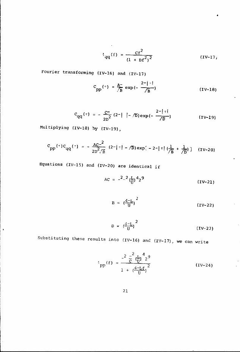
Fourier transforming (iv-16) and {IV-17)

CPP( ^ = TS" exp(--7f~) {IV-i8)

c- 2-iTl cqq(T) = " ^2 (2-i !- /5)exp(- -7r-) (IV.19)

Multiplying (IV-18) by (IV-19),

AC 2 Cpp(T)Cqq(T) = -^Z (2-h|-/ü)expr-2~!T|(X + i)] (IV_20)

Equations (IV-15) and (IV-20) are identical if

Ac - ~2-2^4o9 AC - (ü) 2 (IV-21)

R - f4-L 2 b _ ( U , (IV-22)

D - f^M2 U _ ( U ' (IV-23)

Substituting these results into (iv-16) and (IV-17), we can write

~2cV29 PP d rf 2 (IV-24)

1 + (^)

21

'■rc"1 = —im (IV"25!

The power spectral shapes {IV-24) and (IV-25) are easily pro- duced by linearly filtering white noise. Assume that white noise generators which produce power spectra characterized by the constants Kp and Kq are used; then, since the power spectrum of each process is given by the squared absolute value of the transfer function multiplied by the respective K , (IV-24) and (IV-25) are produced by filters having the transfer functions

(IV-26)

Hq(S> = r 2L ^.2 <IV-27) Ti - ^ • u

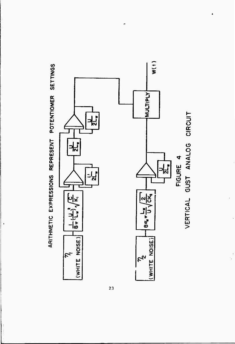
The symbol s is the Laplace transform variable, equal co i2-'f , and the w subscript has been reintroduced in order to avoid later confusion. An analog circuit employing these filters to produce the vertical power spectrum is shown in Figure (4). The diagrams of Reference 35 were used in producing the analog circuits of this report.

3. Generation of the Longitudinal Gust Spectrum

Define u(t) , the longitudinal gust component, to be the product of two independent random processes p(t) and q(t) , both with zero mean value

u(t) = p(t)q(t) (IV-28)

22

(0 o z »—

^

K UJ CO

UJ a. S H o !J

POTE

NTI

ILLJ

L 2 H

Ü tr o

»- r 2 ^ UJ ^ CO N o UJ "1 -J r . 1 . ^ < a. UJ

: / \5 rnr-11 i '

A UJ <

3 . 8 4 ,-, SI en L . I 1... O

a. ^ >

t| <

UJ "* JI= 1«

o

a: H * tf UJ UJ "" CD CD >

? n —1 i ^1 1 L^l

tr UJ UJ < CO CO

o o P^ 2

C4VZ

UJ P" ijj 1- K

i § 23

By (IV-3)

fuu(f) - *pp<f> * »gqCf) (IV-29)

The form of iuu(f) is given by (11-14):

*uu(f) " a u "; 2 {IV-30)

Note that the u subscript of L and a has been suppressed. Following the method of Part (2),

Cuu(T) = Cpp{T)Cqq<T) (IV-31)

CUU{T) = a2exp(-^|T|) (IV-32)

Assume

1 + B

Fourier transforming (IV-33) and (IV-34)

$PP(f) = 777 (IV-33)

$qq(f) = 7^72 (IV-34)

TTA 2nlTl CPP(T) =^eXp(-^-) (IV-35)

TTD 2^

T

Cqq(T) =7feXP(-7r") {IV-3V

24

Equations (IV-31) and {IV-32) will be satisfied if

L 2 2 AD = 16(g) a (IV-37)

B = C^) (IV-38)

Substituting {IV-37) and (IV-38) into (IV-33) and (IV-34)

2 T 2 16^(-)

$pp(f) = —rfri <IV-39) i + (^)

*aa(f) = 2 (IV-40)

1 + (^

These power spectral shapes are produced by passing white noise through filters having the transfer functions

uvü YDKr 4o.. (-r

Hp(s> = 2L s P (IV-41)

1+^r

1 +—«- u

Where Kf and Kg are constants characterizing the power spectra of the white noise generators and the u subscript has been re-

25

introduced. An analog circuit employing these filters to produce the longitudinal gust spectrum is shown in Figure (5).

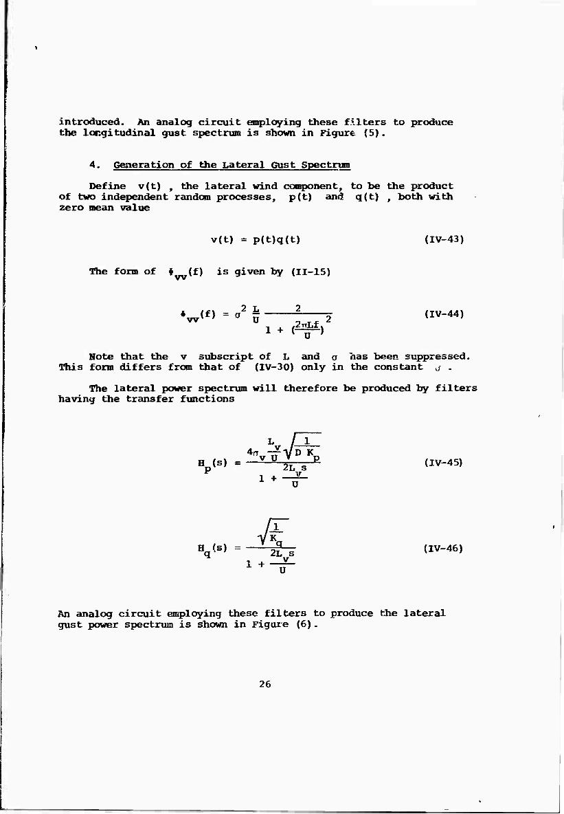
4. Generation of the Lateral Gust Spectnan

Define v(t) , the lateral wind component, to be the product of two independent random processes, p(t) and q(t) , both with zero mean value

v(t) = p(t)q{t) (IV-43y

The form of i (f) is given by (11-15)

*wtf> = °2 ü 7772 <IV-44> i + (^)

Note that the v subscript of L and a has been suppressed. This form differs from that of (IV-30) only in the constant j .

The lateral power spectrum will therefore be produced by filters having the transfer functions

v U V l 4n. V__y__T_ 2L V

VS) = V 2L s P (IV-45) 1 + U

Hq(s) = 2L-7 <IV-46) 1 +

Ü

An analog circuit employing these filters to produce the lateral gust power spectrum is shown in Figure (6).

26

^

=

w

o r >; Z I 1-

_J a. 1— UJ 0) 2

£ 1—

3 K Ü UJ oc 2 o o K

s iD H o O n 1 -J

Z UJ (0 UJ / X

, 1 A . 1 UJ ^

rP ■-r m ■IT ' a: co 0. ^ 3 UJ a: S2 o

••

z c t| y* < z

(0 w UJ

b3

CM 4? o 3

a: a. 1- X <D UJ Z

^^, •""■ i o Ü 1 u UJ 1 _J K CO en UJ o o 2 z fvl 2

I 1- p5" UJ r» UJ

o: t — < 1 ^

1

3: 1 ^^ w

27

> </) o z

1- >- Ul «j w 0.

*2 o: u 3

2 i— u 2 3 o Ü H a: Z u Ü 1- o Q.

o »- -J Z ^U ^U iD < 0) u Q:

Q:

A 4d ( A 41 u <

a: L _i IL 1 to en

C 3 w o z o w 0) UJ tr

(C) Is!* =3

-J <

UJ a. CO t LÜ -J Ü

UJ UJ UJ 2 if) CO I o O . z Q: < P^" UJ

I

P> UJ t X

J J

28

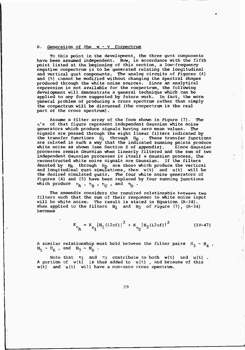
D. Generation of the w - v Cospectrum

To this point in the development, the three gust components have been assumed independent. Now, in accordance with the fifth point listed at the beginning of this section, a low-frequency negative cospectrum is to be generated relating the longitudinal and vertical gust components. The analog circuits of Figures (4) and (5) cannot be modified without changing the spectral shapes produced through the white noise sources. Since an analytical expression is not available for the cospectrum, the following development will demonstrate a general technique which can be applied to any form suggested by future work. In fact, the more general problem of producing a cross spectrum rather than simply the cospectrum will be discussed (the cospectrum is the real part of the cross spectrum).

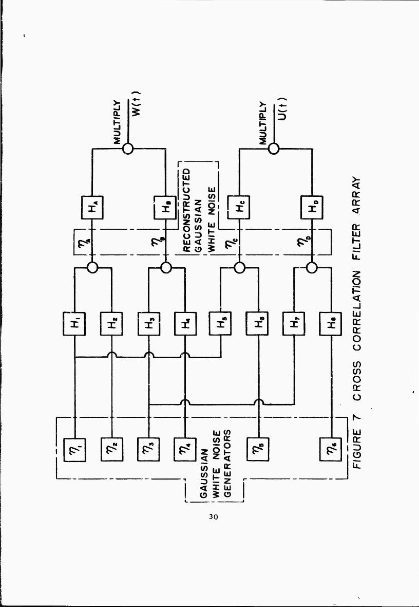
Assume a filter array of the form shown in Figure (7)- The ■p's of that figure represent independent Gaussian white noise generators which produce signals having zero mean values. The signals are passed through the eight linear filters indicated by the transfer functions Hi through Ho . These transfer functions are related in such a way that the indicated summing points produce white noise as shown (see Section E of appendix). Since Gaussian processes remain Gaussian when linearly filtered and the sum of two independent Gaussian processes is itself a Gaussian process, the reconstructed white noise signals are Gaussian. If the filters denoted by H^ through Hj) are those which produce the vertical and longitudinal gust simulations, then w(t) and u(t) will be the desired simulated gusts. The four white noise generators of Figures (4) and (5) have been replaced by four summing junctions which produce *)& > n.ß > ^Q > and ^ •

The apoendix considers the reouired relationshio betwepn two filters such that the sum of their responses to white noise input will be white noise. The result is stated in Equation (A-34). When applied to the filters H^ and H2 of Figure (7), (A-34) becomes

K =K [H, (i2TTf)| + K |H9(i2nf)! (IV-47)

A similar relationship must hold between the filter pairs H^ - H. H5 - K6 , and H7 - Hg . J 4

Note that Tii and "^3 contribute to both w(t) and u(t) . A portion of w(t) is thus added to u(t) , and because of this w(t) and u(t) will have a non-zero cross spectrum.

29

30

This cross spectrum will now be expressed in terms of the filter transfer functions appearing in Figure (7). A somewhat simplified case of this problem is discussed in the appendix, and the desired result in the present case follows directly frcm Equation (A-28). The cross correlation of w(t) and u(t) pro- duced by the circuit of Figure (7) is

Cwu(T) = E{[[(Tll * V - ^2 * h2)] * Vlt *

[[(^ * h3) + [r]4 * h4)] * hB|t •

[[(^ *h5) + (^5 * h6)] *hc]t + T ■

[[(TI3 * h7) + (TI6 * h8)] * hjj. + J (IV_48)

Since the r, of Equation (IV-48) are independent and have zero mean values,

Cwu(T) = E{(T1l * hl * ^'t^l * h8 * Vt + T1 '

E{(Ti3 * h3 * hB)t(T13 * h7 * hD)t + T} (IV-49)

This form is essentially identical to Equation (A-23) since the convolution of two impulse response functions yields the impulse response of the two filters in series. Following the appendix from Equation (A-23) to (A-28) will yield the result, with

i = K. , i = 1 , 2 ,..., 8 . ni 1 '

^(f) = K1K3[H1(-i2TTf)HA(-i2nf)H5(i2nf)Hc(i2TTf)] *

[H1(-i2nf)H^(-i2nf)HT(i2rrf)Hri(i2nf ] (IV-5Gi

31

HA > HB > He , «and HD are the transfer functions of filters required to produce w(t) and u(t) from white noise input. Frcn Part C of this section, with $ = K. i = A ,..., D ,

r], l , 7 ,

Lw 2

V^ 16A/C,K HA'S) r A

i + 2L s

w U

(IV-51)

HB(s)

s /Cl 2-.VK

B

r 2L S./

u _

{IV~52)

47

Kc(s) u u y c K

, 2 C

i + u Ü

(IV-53)

HD(S)

1 + 2L s u

U

{IV-54)

where Cj and C2 are arbitrary positive constants. Substituting (IV-51) through (IV-54) into (IV-50),

K1K,32/7f7 ^ L 2 L ; H, (-i2-s) Hr (i2^s) 1 * /f\ ^ 13 u w. w. _JJ. lx 1_5 : ^ wu^ ' yK. K K K vu' lU; 4rTL..s 4"L..s

A"B C D (1 - i- w U ) (1 + i"

u u

[-i2ns H3{-i2TTS) H7(i2-s)]

4-TL S 2 4-L s (l-i-^) (l + i-^)]

(IV-55)

32

The transfer functions H^ through Hs can now be chosen. The only requirement is that Equation (IV-47) must hold for each pair Hj - H? , H3 - H4 , H5 - H5 , and H7 - Hg . Note that H2 H4 , H^ , and Hg do not appear in the cross spectrum, Equation

Many filters could be chosen, all of which would satisfy the requirement of a low-frequency negative cospectrum. Let

Hi(s! =-!-T-r^ 'IV-56i

o L 2 s -/— [^ - (2-^) ]

V K2 h

H2(s) - (1 + as) {IV~57>

KD 2L 2

ir(1+-[rs) H.(s) = 5 {IV-58)

(1 + asp

H^s) = 2 5 (IV-59) (1 + as)^

H5(s) = TT-^ (IV-60)

33

fKc 2 L 2 • »/Jf" ! a - (2—) j

H6(s) -^"^ 1 ^ as (IV-61)

^. 2L

(1 +~^s) H7(3)--^—YT-ST-— ':iv-62)

V*3

s V^ - (2^)2] H8(s) = 1 + as

(IV-63)

L 2 L ^(f) = - 32/2auaw(f) (lf)[(1-i2TTaf)

1(1+i2^f)] *

^ (IV-64) (l-i2TTaf) {l+i2rTaf)

Note that the shape of the cross spectrum is now a function of only a .

The reduction of Equation (IV-64) to algebraic form is rather complicated. If the equation is first Fourier transformed, and then reduced by carrying out the resulting correlations, the inverse Fourier transform will yield the desired result. When these steps are followed, the real part of Equation (IV-64) is finally shown to be

- 2/2CT a L 2 L r, , -. , £.2-, x IfK u w, w. . u. jl + 3(TTaf 1 $c (f) - 2 (ir) iij)r, x / "2,2 (IV-65) wu a 11 + (^af) ]

34

en 2 Lü

00 Q

UJ _| (t < 3 or o K ll Ü

LÜ CL (/) o Ü

35

If Lu is chosen equal to Lw and a is set to 3.5 L^/U , the cospectral form becomes as shown in Figure 8, which has been plot- ted for direct comparison with meteorological data.

This completes the analog circuit derivation. The next section of this report summarizes the above development, discusses the simulation, and presents the final analog diagrams.

36

SECTION V

REVIEW AND DISCUSSION OF DEVELOPMENT

This section discusses the non-Gaussian turbulence simulation developed in Section IV. Part A summarizes Section IV for those who do not wish tc follow the mathematical treatment. Part B considers some practical aspects of the simulation and suggests possible simplifications.

A. Review of Development

Section III of this report discusses the characteristics of various turbulence simulation techniques and finds that the filtered white noise model offers both versatility and simplicity. However, the probability density produced by the simulation is Gaussian, and therefore not representative of rea? turbulence.

Section IV extends the filtered white noise method to include a non-Gaussian probability distribution. Six desirable features which the new simulation should have are listed at the beginning of that section. These features are:

1. An analog network is to produce three simultaneous random processes. These three processes are to represent the three orthogonal gust components occurring at a point (such as the center of gravity of a vehicle).

2. Each component should have a probability density character- ized by the modified Bessel function of order zero, K0 .

3. The simulated gust time histories are to have the same normalized spectra as were chosen in Section II to represent atmospheric turbulence. The scale length of each component should be an independent variable.

4. The rms intensity of each component should be an independent variable,

5. A negative low-frequency correlation should exist between the vertical and longitudinal gust components.

6. The analog circuit should be as uncomplicated as possible, using Gaussian white noise generators and linear filters.

Statement number two requires that the simulation produce time histories with modified Bessel function probability densities. Section IV shows that this probability density is produced whenever two independent Gaus ian processes with zero mean values are multi-

37

pl^ed. Therefore, a fundamental feature of the non-Gaussian simu- lation is the multiplication of Gaussian processes. Each of the three simulated gust components is produced in this way. Once the use of multiplication is established as the method of producing gust components, the remainder of the simulation technique follows directly.

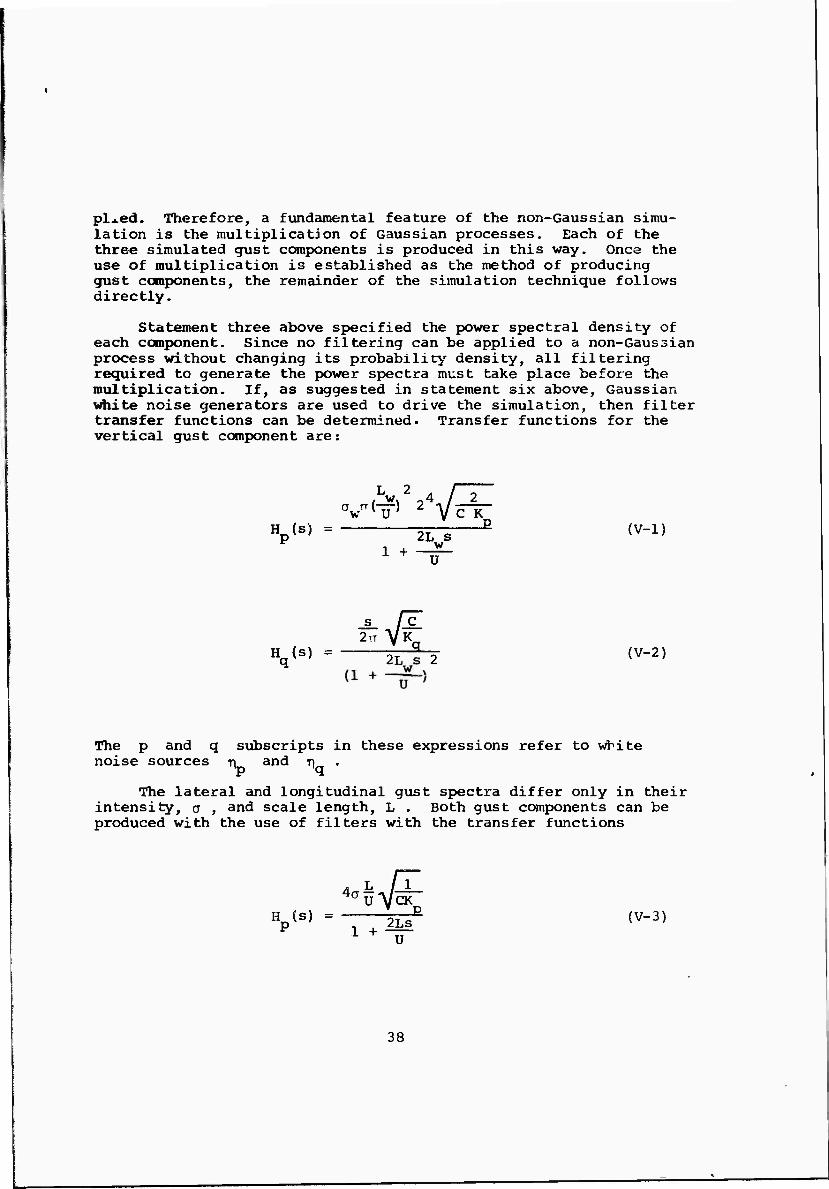
Statement three above specified the power spectral density of each component. Since no filtering can be applied to a non-Gaussian process without changing its probability' density, all filtering required to generate the power spectra must take place before the multiplication. If, as suggested in statement six above, Gaussian white noise generators are used to drive the simulation, then filter transfer functions can be determined. Transfer functions for the vertical gust component are:

L 2 .

v^ 2 V^r VSi = 2L-i K ^"^ 1 + ^f-

s fc 2" VK

Hq(s) = r~^ (V~2)

The p and q subscripts in these expressions refer to white noise sources n and r\

V «I The lateral and longitudinal gust spectra differ only in their

intensity, a , and scale length, L . Both gust components can be produced with the use of filters with the transfer functions

4a u IT UVCK

Vs) = ~—ZLT (v-3) 1 + U

38

^ Hq(s)=rriLi (v-4)

U

Again p and q refer to white noise sources ^Ip and "nq • The symbols L and a apply to either the lateral or longitudinal gust component as the case may be. Analog circuit diögrams of the three gust component simulations are presented in Figures 4, 5f and 6.

Note that these filters account for the rms of each component independently. This feature satisfies the requirement of statement four at the beginning of this section.

Independent simulations of the three gust components have thus been obtained. It remains only to introduce the cospectral relationship between the vertical and longitudinal gust components. The circuit of Figure 7 illustrates a very general method of obtain- ing this result. The output signals w(t) and u(t) in that figure represent the vertical and longitudinal gust components. The filters Hft through Hp represent the filter pairs mentioned above [Equations (V-l) through (V-4)] which produce these components. Since the lateral component is independent, it does not enter into the cospectrum problem. The filters H^ through UQ are chosen so that Gaussian white noise is produced at the indicated summing junctions. The white noise generators of Figures 4 and 5 are thus replaced by the filter array to the left of these summing points. Mote that the white noise sources ^i and ^3 contribute to both w(t) and u(t) . These two noise sources introduce the correlation between w{t) and u(t) .

H, through Hfi are chosen to be

Hl(s) = T^i (v-5)

Vk. _ L 2

H2(S) = j—r^ ^v-6)

39

V'KT 2L 2

H3(s) = ^ (V-.7) (1 + as)^

v^[V2[a2 - (2^,2] + s\/^ (2^)4> H (s) = 5 — = (V-8)

(1 -5- asp

v5 H5{S) " 1 + as (V-9)

2L (l+^s,

Vft-2 - ^ H6(s) = 1 + as <v-10)

nC 2L r D /-. . U K (1 +-üiis)

H7(s) = -^-T^ (V-11)

s V^[a2 - (^,2] H

8<s) ' ' '6 1 ^ as (V-12)

If it is assumed that the scale lengths of the three gust components are equal, then the cospectrum produced by the circuit of Figure 7 is

40

$ (f) = r^<if) (if)[1 + 3(^fl j (v-i3) cwu a^ U ü [1 + (naf)2]2

The magnitude of a in Equation {V-13) can be chosen from a range of values. If the scale lengths are assumed equal and a is chosen to equal 3.5 L/U , the cospectral form becomes as plotted in Figure 8.

All of the components of the turbulence simulation have now been determined. Figure 9 and the accompanying table present the complete analog circuit. The diagrams of Reference (35) have been used to translate the filter transfer functions listed above into the analog circuit of Figure 9.

B. Discussion of Simulation

Several aspects of the simulation and its development will now be considered.

1. Simplicity

Six desirable features of a turbulence simulation are presented at the beginning of this section and in Section IV. The first five of these points have been satisfied by the preceding development. However, the sixth item has not been considered. This item states that the simulation should be uncomplicated, using Gaussian white noise generators and linear filters wherever possible. Though the second half of the statement has been satisfied, the final circuit as presented in Figure 9 can hardly be called uncomplicated. How- ever, some simplification is possible.

For example, Vrj and tis of Figure 9 are actually unnecessary. These two noise generators can be replaced by connections to T^ and "512 without affecting the independence of the lateral gust component. Thus, only six white noise generators are essential.

The use of a less complicated cross correlation technique might permit additional noise generators to be deleted from the circuit, resulting in a more compact simulation. It is also possible that certain choices of the parameters U , L , and K will allow some simplification.

2. Simulation of the "Patchy" Turbulence Structure

The multiplication technique used in this report was initially suggested by the "patchy" structure of turbulence. This led to the

41

^m

FIGURE 9 FINAL ANALOG CIRCUIT

CIRCLED NUMBERS REFER TQ TABLE I

n

7} ARE GAUSSIAN WHITE NOISE SOURCES "1

J V(t)

w 42

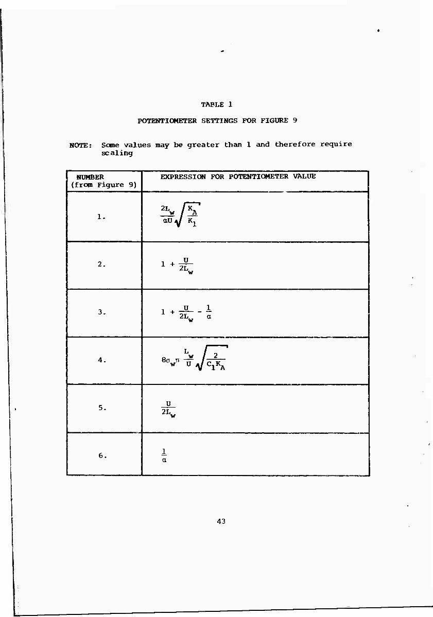
TABLE 1

POTENTIOMETER SETTINGS FOR FIGURE 9

NOTE: Some values may be greater than 1 and therefore require scaling

NUMBER (from Figure 9)

EXPRESSION FOR POTENTIOMETER VALUE

1. 2L /K ' w / A aUV Ki

2. l+^

3. -<-i

4. 8„ n ^ / 2 ' "V u VcA

5. u 2Lw

6. 1 a

43

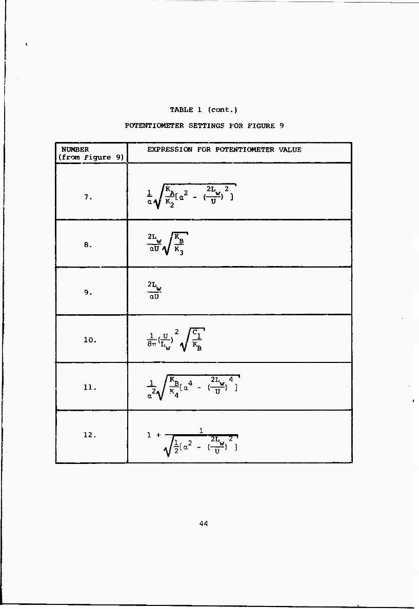
TABLE 1 (cont.)

POTENTIOMETER SETTINGS FOR FIGURE 9

1 NUMBER [(from Figure 9)

EXPRESSICW FOR POTENTIOMETER VALUE 1

1 7- , /K,. _ 2L 2 '

8. W / B 1 aU Y K3

9. 2L f w au

] 10. 1(ü)2/Cl'1

I 11- ^*-'-'*''■

i i2.

1>2-'"W-

44

TABLE 1 (cont.)

POTENTIOMETER SETTINGS FÜR FIGURE 9

NUMBER (from Figure 9)

EXPRESSION FOR POTENTIOMETER VALUE

13. _ a-V2[a ^ ( u ) 3 1 + r-r—n 2 »

aV2Ca + (■lf, ]

14. 2L fKT

u/ C aU^ K1

15. ^^

16. 1+ " -1

^u a

17. , /K^ _ 2L 2 '

18. 20VC2K2

19. u 2Lu

45

TABLE 1 (concluded)

POrarPIOMETER SETTINGS FOR FIGURE 9

NUMBER (from Figure 9)

EXPRESSION FOR POTENTIOMETER VALUE

20. aüVK3

21. u FT

22. , /k,, , 5L 2 •

i^0 "(°u, ]

23. 2''vVc3K7

24. Ü 2Lv

25. iF1

u rs 2LvVK8

46

ciioicc of a modified Bessel function probability density. Though this probability density has been retained, the original conception of simulating each gust component by the product of a turbulence function and an intensity function-has become somewhat obscure. It is possible that a differen*: method of introducing the cross corre- lation would result in a more obvious analog representation. There is also some question as to whether or not "patchy" turbulence will be realisLically simulated if only the power spectral density and probability density are reproduced. The filter transfer functions derived In Section IV of this report are not unique. General forms were assumed for the functions and these wore shown to satisfy the desired equations. Many of the constants, particularly those speci- fying cutoff frequencies were arbitrary. It does not seem likely that satistically identical results would be obtained if these constants were changed. For example, it is possible that they in some way specify the average patch size of the turbulent field. This is a question which should be studied in future work.

3. Ideal Circuit Elements

The preceding development has assumed that all circuit elements behave in an ideal manner. This assumption is justified as far as the linear analog equipment is concerned, but the multipliers and white noise generators may present some difficulties.

White noise generators are necessarily non-ideal. The power spectral density produced by any physically possible noise source cannot be simply a constant, as has been assumed in the preceding derivations, but must fall to zero at high frequencies. In other words, the power spectrum can be flat over only a finite frequency range. Fortunately, low-pass filtering is used in the simulation. Consequently, only frequencies below about 15 cycles per second are important. Higher frequencies are not passed by the filter array. Therefore, any white noise source which produces a flat spectrum below about 15 cycles per second will be acceptable.

Another important restriction placed upon the noise generators is that they produce signals with zero mean values. If this condition is not met, the probability density will no longer be characterized by tc0 and the spectrum equations will contain additional terms. In other words, the derivations of this report will no longer apply in the strict sense. Of course, a mean value will always be present in physically realizable equipment. Therefore an acceptable mean value limit must be determined. Though this problem has not been studied in detail, it appears that effects upon the power spectra and cospectrum are negligibly small if the largest mean value can be held to less than one or two percent of the smallest white noise rms value. The effect of non-zero mean values on the probability density has proved somewhat more difficult to analyze. It seems probable that the presence of a mean value in the Gaussian noise signals will produce a process which is neither Gaussian nor K0

47

but one of a family of probability densitie.3 lying between these extremes. (Perhaps one of these intermediate distributions in actually more representative of turbulence than the K0 dis.;:.i- bution, a possibility which should be studied in future work.) If the largest mean value is held to less than one or two percent of the smallest white noise rms value it should not seriously change ehe probability density distribution.

The quality of the analog multipliers is another important consideration. Any non-ideal operation of these units will affect both the spectral relationships and the probability densities. No analysis of this problem has been undertaken; however, it seems certain that the accuracy currently available in analog multipliers (0.3 - 0.4% of full scale output) is more than sufficient to pro- duce good results.

The complete analog circuit of Figure 9 has been constructed and appears to operate as predicted although the lack of high quality multipliers and noise generators compromised the results. A statistical analysis of the generated signals has not been made.

4. Extension to Spatial Distribution

This report has not considered any methods of extending the simulation to include the effects of spatially distributed turbu- lence. For example, the simulation described here cannot produce a vehicle rolling moment due to the distribution of the vertical gust component along the wing span. Although such an extension is certainly possible, it is clearly going to be difficult in view of the complications already experienced. In order to introduce a minimum amount of additional complication, a careful study of alter- natives should be made before a particular method of extension is adopted.

5. Restrictions on Vehicle Flight Path

It is important to note that the spectral equations used in this report are, in general, valid only for flight parallel to the mean wind vector. Although this restriction permits simulation of normal "into the wind" take-off and landing as well as hover, it does not permit simulation of crosswind flight. If the direction of flight is taken to be across the mean wind, the spectral forms may be some- what different (see for example Reference 36). Since there is presently little information on such effects, no attempt has been made to account for them here.

48

SECTION VI

SUMMARY

Section II of this report discusses those statistical prop- erties of low altitude atmospheric turbulence which must be con- sidered in a piloted flight simulator. The homogeneity, stationarity, probability density, rms intensity, power spectral densities, and cross spectral densities are all considered. The unusual feature of the chosen representative forms is a non-Gaussian probability density, characterized by the modified Bessel function of the second type of order zero, iC0 . The choice of this form is based upon an argument arising from the "patchy" structure of turbulence and upon experimental measurements typified by Figure 1. Figure 2 presents a comparison of the Gaussian and K0 distributions.

Section III of this report considers the characteristics of several, turbulence simulation techniques. The filtered white noise, recorded time history, and sum of sine waves methods are discussed. The filtered white noise model, which simulates turbulence by lin- early filtering the output of a Gaussian white noise generator, is found to offer both simplicity and versatility. Unfortunately, it does not reproduce the non-Gaussian nature of turbulence.

Sections IV and V ext^ ^d the filtered white noise technique to include the modified Besse . function probability density. It is found that the product of independent Gaussian processes will yield the desired probability density, and that linear filtering can be used to obtain the desired power spectral densities. A very general method of introducing cross correlation between the gust components is also developed. The final analog circuit of the simulation is presented in Figure 9 and Table 1. Some possible simplifications in the circuit are discussed in Section V.

The three outputs which appear in Figure 9 represent the three orthogonal gust components of low altitude atmospheric turbulence. The rms intensity and scale length of each component are independent variables. The probability density, power spectral densities, and cross spectral density of the simulation are presented in Figure 2, 3, and 8 respectively.

49

REFERENCES

1. Lumley, J. L., and Panofsky, H. A., The Structure of Atmos- pheric Turbulence. Monographs and Texts in Physics and Astronomy, Vol. 12, New YorH: John Wiley and Sons, Inc, 1964,

2. Volkov. Iv. A., Kukharets, V. P., and Tsuang, L. R., "Turbu- lence in the Atmospheric Boundary Layer Above Steppe and Sea Surfaces,"' Akademiia Nauk SSSR. Izvestiia. Fizike Armosfery i Qkeana. Vol. 4, October 1968.

3. Anon., "TSR.2 Integrated Weapons Svstem," Aircraft Engineering. Vcl. 35, No. 11, 1963.

4. Allan, R. M., "Results of a Flight investigation on Clear Air Turbulence at Low Altitude Using a Meteor Mk:7 Aircraft," Great Britain Aeronautical Research Council, Current Paper 329, X957.

5. Bullen, N. I., "A Review of Information on the Frequency of Gusts at Low Altitude," Great Britain Aeronautical Research Council, Current Paper 873, 1966.

6. Frenkiel, F. N., and Klebanoff, P. S., ,:Higher Order Correla- tions in a Turbulence Field, Physics of Fluids. Vol. 10, March 1967.

7. Dutton, J. A., Thompson, G. J., Capt. USAF, and Deaven, D. G., "The Probabilistic Structure of Clear Air Turbulence—Some Observational Results and Implications," in: Boeing Scientific Research Laboratories. Symposium on Clear Air Turbulence and Its Detection. Seattle. Washington. August 14-16. 1968. Proceedings. Boeing Scientific Research Laboratories, Seattle, 1968.

8. Bullen, N. I., "Aircraft Loads in Continuous Turbulence," North Atlantic Treaty Organization, AGARD Report 116, April- May 1957.

9. Abramowitz, M., and Stegun, I. A., Ed., Handbook of Mathemati- cal Functions With Formulas. Graphs, and Mathematical Tables, National Bureau of Staidards Applied Mathematics Series 55, Washington: U. S. Government Printing Office, 1964.

10. Bullen, N. I., "Atmospheric Turbulence in Relation to Aircraft," International Congress for Applied Mechanics. Proceedings, Vol. 3, 1956. ^

50

li. Batchelor, G. K., The Theory of Homogeneous Turbulence. Cambridge Monographs on Mechanics and Applied Mathematics, Cambridge, University Press, 1953.

12. Novikov, E. A., and Stewart, R. W., "The Intermittency of Turbulence and the Spectrum of Energy Dissipation Fluctua- tions," Akademiia Nauk SSSR. Izvestiia. Seriia Geofizicheskaia. March 1964.

13. Elderkin, C. E., "Experimental Investigation of the Turbulence Structure in the Lower Atmosphere," Battelle Northwest Report BNWL-329, December 1966.

14. Haitiner, G. J., and Martin, F. L., Dynamical and Physical Meterology. New York: McGraw-Hill, 1957.

15. Seckel, E., Miller, G- E., and Nixon, W. B., "Lateral- Directional Flying Qualities for Power Approach," Report 727, Princeton university, September 1966.

16. von Karman, T., "Progress in the Statistical Theory of Turbu- lence," Turbulence Classic Papers on Statistical Theory. New York: Interstate Publishers, Inc., 1961.

17. Gault, J. D., and Gunter, D. E., Jr., "Atmospheric Turbulence Considerations for Future Aircraft Designed to Operate at Low Altitudes," Paper 68-216, American Institute of Aeronautics and Astronautics, Aircraft Design for 1980 Operations Meeting, Washington, D. C, February 1968.

18. Miller, D. P., and Vinge, E. W., "Fixed-Base Flight Simulator Studies of VTOL Aircraft Handling Qualities in Covering and Low-Speed Flight," Technical Report AFFDL-TR-67-1D2, Air Force Flight Dynamics Laboratory, Air Force Systems Command, Wright- Patterson Air Force Base, Ohio, January 1968.

19 Dryden, H. L., "A Review of the Statistical Theory of Turbu- lence, " Turbulence Classic Papers on Statistical Theory. New York: Interstate Publishers, Inc., 1961.

20. von Karman, T., and Howarth, L., "On the Statistical Theory of Isotropie Turbulence," Proceedings. Royal Society of London. Series A, 164, 1938. ~ ^^^- ._

21. Fichtl, G. H., "Characteristics of Turbulence Observed at the NASA 150-meter Meteorological Tower," Journal of Applied Meteorology. Vol. 7, Ot^ober 1968.

22. Stone, C. R., and Skelton, G. B., "Investigation of the Effects of Gusts on V/STOL Craft in Transition and Hover," Interim Report, Contract No. F33615-67-C-1563, Air Force Flight

51

Dynamics Laboratory, Research and Technology Division, Air Force Systems Command, Wright-Patterson Air Force Base, Ohio. July 1967.

23. Chalk, C. R., "Fixed-Base Simulator Investigation of the Effects of La and True Speed on Pilot Opinion of Longitudinal Flying Qualities," Technical Documentary Report ASD-TDR-63-399, Flight Dyneimics Laboratory, Research and Technology Division, Air Force Systems Command, Wright-Patterson Air Force Base, Ohio, November 1963.

24. Bray, R. S., and Larsen, W. E., "Simulator Investigation of the Problems of Flying a Swept Wing Transport Aircraft in Heavy Turbulence," Conference on Aircraft Operating Problems, Langley Research Center, May 1965.

25. Hall, A. W., and Harris, J. E., "A Simulator Study of the Effectiveness of a Pilot's indicator which Combined Angle of Attack and Rate of Change of Total Pressure as Applied to the Take-Off Rotation and Climbout of a Supersonic Transport," National Aeronautics and Space Administration, Technical Note D-948, September 1961.

26. Adams, J. J., "An Analog Study of an Airborne Automatic Landing- Approach System," National Aeronautics and Space Administration, Technical Note D-105, December 1959.

27. A'Harrah, R, C., "Low-Altitude, High Speed Handling and Riding Qualities," Paper 63-229, American Institute of Aeronautics and Astronautics, Summer Meeting, Los Angeles, California, June 1963.

28. Stenning, A. T., and Dolan, J. A., "Lateral Directional Simulation of the CL-84 V/STOL Aircraft in the Transition Regime," Paper 64-806, American Institute of Aeronautics and Astronautics, Canadian Aeronautics and Space Institute, Joint Meeting, Ottawa, Canada, October 1964.

29. Soliday, S. M., and Schohan, B., "Performance and Physiological Responses of Pilots in Simulated Low-Altitude High-Speed Flight," Aerospace Medicine. Vol. 36, February 1965.

30. Hirsch, D. L., and McCormick, R. L., "Experimental Investigation of Pilot Dynamics in a Pilot Induced Oscillation Situation," Paper 65-793, American Institute of Aeronautics and Astronautics, Royal Aeronautical Society, and Japan Society for Aeronautical and Space Sciences, Aircraft Design and Technology Meeting, Los Angeles, California, November 1965.

52

31. Davenport, W. B., Jr., and Root, W. L., An Introduction to the Theory of Random Signals and Noise. New York: McGraw-Hill, Inc., 1958.

32. Bracewell, Ron, The Fonrier Transform and Its Applications. New York: McGraw-Hill, Inc., 1965.

33. Solodovnikov, V. V., Introduction to the Statistical Dynamics of Automatic Control Systems. New York: Dover Publications, Inc., 1960.

34. Watson, G. N... A Treatise on the Theory of Bessel Functions. Second Edition, The Cambridge University Press, 1958.

35. Jackson, A. S., Analog Computation. New York: McGraw-Hill, 1960.

36. Burns, A., "Power Spectra of LOW Level Turbulence Measured from an Aircraft", Great Britain, Aeronautical Reoearch Council Current paper 733, April 1963.

53

APPENDIX

DERIVATION OF GENERAL STATISTICAL RELATIONSHIPS

Section IV of this report develops a turbulence simulation Which employs the multiplication of independent random processes. This appendix derives the statistical relations upon which tho

development of Section IV is based. Functions derived, in the order of their development, are:

1. Probability density of the product of two independent random processes in terms of the probability densities of the given processes.

2. RMS intensity of the product of two independent random processes in terms of the rms intensities of the given processes.

3. Power spectral density of the product of two independent random processes in terms of the power spectral densities of the given processes.

4. Cross spectrum of two random processes, each the product of two linearly filtered, independent, white noise signals.

5. Reconstruction of white noise from a sum of linearly filtered, independent, white noise signals.

References 31, 32, and 33 may be of some help in understanding the following derivations.

A. Probability Density of the Product of Two Independent Random Processes

Let r(t) be the product of two continuous, independent random processes, p(t) and q(t) .

r(t) = p(t)q(t) (A-l)

Assume that the probability density functions of p(t) and q(t) are given by Pp(x) and Pq{x) respectively. Then the probability that p(t) and q(t) take on particular values is

[probability that p = x] = PD(x)dx (A-2)

[probability chat q = y] = Pa{y)dy

Since p(t) and q(t) are independent processes, the proba- bility that they take on particular values simultaneously is simply the product of the individual probabilities.

54

probability that

p = x and q = y

simul taneously

= Pp(x)Pq(y)dbcdy {A-3)

Let It (z) be the probability distribution of r(t). Then the probability that r(t) takes on some value less than or equal to z is given by

I»r(z) = JJP (x)P (y)dxdy (A-4)

Where F denotes that region of the x - y plane in Which the relation xy < z is true. Supplying limits for (A-4),

I,r(z) = I 5 PD(x)Pa(y)dxdy + J J P (x)P (y)dxdy y=0 x=-«i> F H y=— x=z/y p H

Then P (x) is obtained by differentiating (A-5)

(A-5)

Pr(z) = I[Pp(xJPqCf) + Pp(-x)Pq(.f)^ (A-6)

Equation (A-6) relates the probability densities of two independent functions, p and q , to the probability density of their product, r .

B. HMS Intensity of the Product of Two Random Processes

Let r(t) be the product of two independent random processes, p(t) and q(t) , with zero mean values.

rCt) = p(t)q(t)

Prom (DEF-14) the rms intensity of r is

{A~7)

_ Lim ar T->a. vHr

(t)2dt (A-8)

55

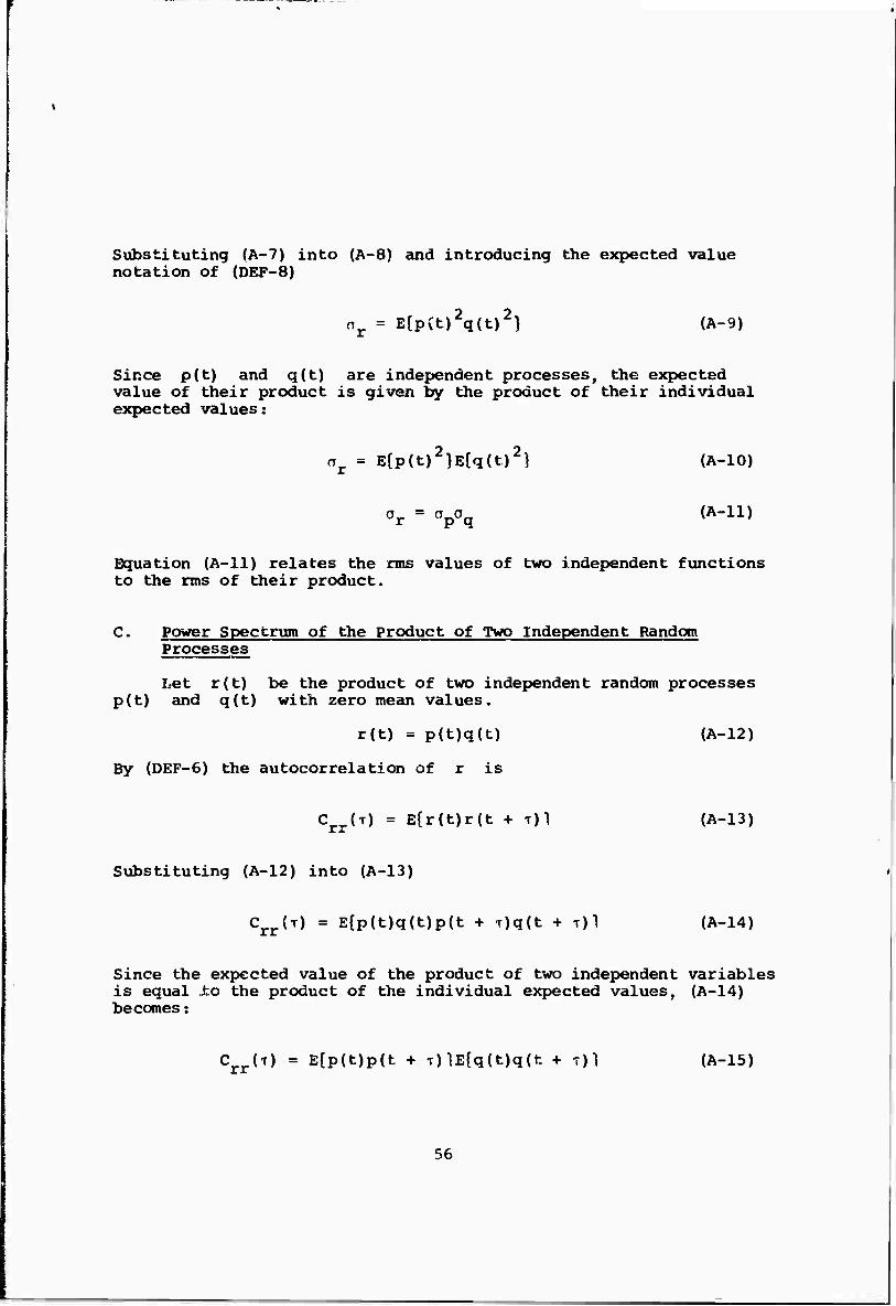
Substituting (A-7) into (A-8) and introducing the expected value notation of (DEF-8)

nr = E{p(t)2q(t)2} (A-9)

Since p(t) and q(t) are independent processes, the expected value of their product is given by the product of their individual expected values:

oT = E{p(t)2}E{q(t)2) (A-10)

or = apaq (A-ll)

Equation (A-ll) relates the rms values of two independent functions to the rms of their product.

C. Power Spectrum of the Product of Two Independent Random Processes

Let r(t) be the product of two independent random processes p(t) and q(t) with zero mean values.

r(t) = p(t)q{t) (A-12)

By (DEF-6) the autocorrelation of r is

Crr(T) = E{r(t)r(t + T)1 (A-13)

Substituting (A-12) into (A-13)

Crr(T) = E{p(t)q(t)p(t + T)q(t + T)1 (A-14)

Since the expected value of the product of two independent variables is equal ±o the product of the individual expected values, (A-14) becomes:

Crr(T) = E{p(t)p(t + T)lE{q(t)q(t + T)1 (A-15)

56

By (DEF-6)

Crr(T) = CpP(T)Cqq(T) (A"16)

By (DEF-17) the power spectral density of r is

*rr^ = I CPP(T)Cqq{T)e"i2nfTdT (A"17)

Equation (A-17) states that $rr is given by the Fourier Transform of the product CppCqq . It is well known that the Fourier trans- form of a product becomes a convolution in the frequency domain (see, for example, Reference 32). Equation (A--17) thus becomes:

♦ rr(f) = Ppptf - ß)*qq(ß)dP (A"18)

or, by (DEF-1),

Wf> = *pp * *qq (A-19)

Equation (A-19) implies that the power spectral density of the product of two independent random variables is given by the convo- lution of their respective power spectral densities.

D. Cross Spectrum of Two Products of Random Processes

Let r(t) and q(t) be products of random processes with zero mean values

r(t) = m1(t)n1(t) (A-20)

q(t) = m2(t)n2(t) (A-21)

By (DEF-6), their cross correlation is

57

C (T) = E{in1(t)n1(t)m2{t + T)n2(t + T> 1 (A-22)

Let ra^Ct) and 102 (t) both be produced by passing a signal mit} through linear filters with impulse-response functions h,,, (t) and h,,, (t) respectively. Let ni(t) and n2(t) be

similarly produced from a signal n(t) , which is independent of m{t) .

Crq(T> = Ef ^j * ^t^nt, * ^ t * r^f % * n)t(hn2 * n,t + T

1

(A-23)

Since all functions in (A-23) are physically possible, all integrals in that expression must converge uniformly.

Expanding the convolution notation and changing the order of integration then gives

cialj) = JJ^m (a)h (ß)E{m(t - a)m{t + T - ß) }dadp "l "^

• t[hn (a)hn (ß)E{n(t - a)n(t + T - ß)}dadß a ni n2

By (DEF-6),

Crq(T) ^ :rjfhm1

(a)hn2(ß,Cn«(T + a " e)dad3 "

* LV<*>hn <ß,Cnn(T + a- ß)dadß —00 i 2

(A-24)

(A-25)

58

Fourier transforming (A-25)

lrq(f> = fJJV^V^ J" C™n(T + a ' P>e"i2TTfTdTdad^ * ^ -co i 2 —•

fJI11« (a>h« W J Cnn^ + « " ß)e"i2TTfTdTdadßl ii ni n2 i» nn

{A-26)

Introducing the change of variable Y = T + a - ß in (A-29) gives

♦ ^(f) = [♦„,„,(f)H (-i2TTf)Hn {i2TTf)]*[fnn(f)Hn (-i2TTf)Hn (i21Tf)] rq mm m, m^ nn n, n^ {A-27)

If m(t) and n(t) are white noise signals, then their power spectra are merely constants:

»(f) = K K [H (-i2TTf)H (i2TTf)]*[Hn (-i2TTf)H {i2TTf) ] {A-28) rq m n ni,v m^ n, n-

Equation (A-28) expresses the cross spectrum of two random processes, each the product of two linearly filtered, independent, white noise processes in terms of the filter transfer functions.

E. Reconstruction of White Noise from a Sum of Linearly Filtered White Noise Signals

The correlation technique to be described in Section IV of this report will require knowledge of a method of constructing white noise from a sum of non-white noise sources.

Let r(t) be the sum of two independent signals p(t) and q(t), each with zero mean value:

r(t) = p(t) + q(t) (A-29)

By (DEF-6), noting that p(t) and q(t) are independent.

59

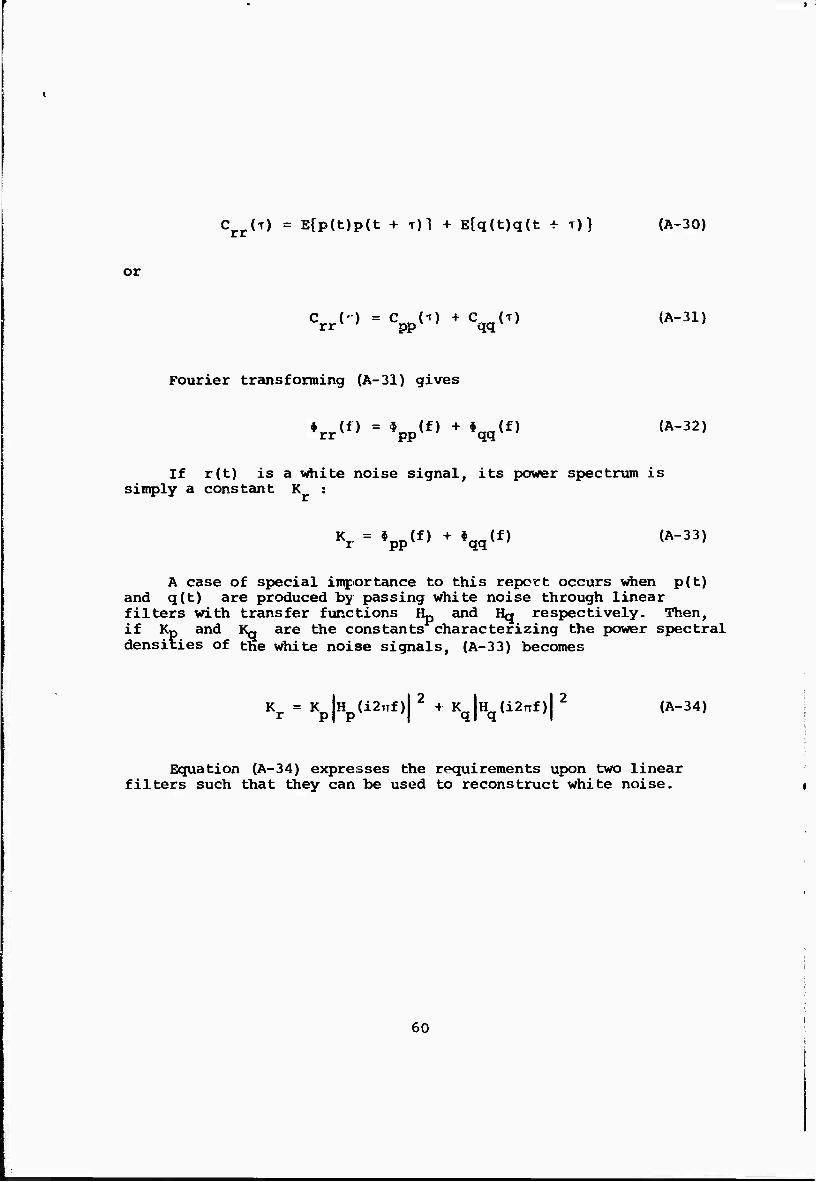
Crr{T) = E{p(t)p(t + T)1 + E{q(t)q(t -!- T)} {A-30)

or

C (') = C (T) + C (T) {A-31) rrx ' PP Qq

Fourier transforming (A-31) gives

♦rr(f) = *pp(f) + *qq(f) (A-32)

If r(t) is a white noise signal, its power spectrum is simply a constant K :

Kx = *pp(f) + *qq(f) (A-33)

A case of special importance to this report occurs when p(t) and q(t) are produced by passing white noise through linear filters with transfer functions Hp and Hq respectively. Then, if Kp and Kg are the constants characterizing the power spectral densities of the white noise signals, (A-33) becomes

Kr = Kp|Hp(i2TTf)| 2 + Kq|Hq(i2TTf)|

2 (A-34)

Equation (A-34) expresses the requirements upon two linear filters such that they can be used to reconstruct white noise.

60

Unciasslfled

Security q«»m«fic«tioB

DOCUMENT CONTROL DATA -R&D fS+CMJIy rlM«<f(f tian ol Hi;», body o/a6<fmcland Inömtlnt mnnauUcm mutt br anttwd mh—t Of ovyrmll report la elmmmlHwnt)

ORICIMATIMC ACTIVITY t'CoiparaM au*<rj

University of Washington, College of Engineering Department of Aeronautics & Astronautics Seattle, Washington 98105

im. REPORT «ECURITT CLASSIFICATION

Unclassified tb. CROUP

N/A 1 REPORT TITLt

A Non-Gaussian Turbulence Siaulatlon

4 OESCRIPTivc MOTES (Typ» af mpert tnd inclu*ir* dmlrr)

Final Technical Report, June 1967 - June 1969 S AUTMORISi (rim mIMIm Inlllml. laml I

Paul M. Reeves

• REPORT OATC

June 1969 7«. TOTAL NO. OF -^ACES

76 76. NO. OF MCFl

35 %m, CONTRACT OR 6RAMT MO

F33615-67-C-1851 6. PROJECT NO IIJ-IQ

cTask No. 821907

dWork Unit No. 821907009

9m. ORIGINATOR'S REPORT NUMBERI*)

AFFDL-TR~69-67

OTHER REPORT NOISI (Ar.jr otfi'r Oil* import)

None

mmtban Aar mmr bo mmmtgtmä

10- DISTRIBUTION STATEMENT

This document has been approved for public release and sale; its distribution Is unlimited.

II. SUPPLEMENTARY NOTES II SPONSORING MILITARY ACTIVITY

Air Force Flight Dynamics Laboratory Air Force Systems Conmand Wright-Patterson Air Force Base. Ohio

13. ABSTRACT

A comparison of the statistical properties of low altitude atmospheric turbulence and the characteristics of presently used simulation techniques shows that these techniques do not satisfactorily account for the non-Gaussian nature of turbulence. A non-Gaussian turbulence simulation, intended to be used in conjunction with piloted flight simulators, is developed.

The simulation produces three simultaneous random processes which represent the three orthogonal gust components. The probability distribution of each component is char- acterized by the modified Bessel function ic , and the power spectral densities suggested by H, L. Dryden are used in a slightly modified form. The rma in- tensity ind scale length of each component are independent parameters. A general method of Introducing cross spectra between components is demonstrated.

The multiplication of independent random processes is used to generate each of the gust components. Gaussian white noise generators, analog multipliers, and linear filters are used throughout the simulation. A complete analog circuit diagram is presented.

DD FORM i NOV es 1473 Unclassified

Security CIdssification

UnclasHtflftd Security CUssirication

KCV monot ROLE WT

V/STOL

Turbulence

Gusts

Low Altitude

Matheaatlcal Models

Unclassified Security Classification