o large scale maintenance n evolutionary …

DAAAM INTERNATIONAL SCIENTIFIC BOOK 2011 pp. 495-512 CHAPTER 40

OPTIMISATION OF LARGE SCALE MAINTENANCE

NETWORKS WITH EVOLUTIONARY PROGRAMMING

KOTA, L.

Abstract: This study develops a single phase algorithm for the fixed destination multi-depot multiple traveling salesman problem (MD-MTSP) with sub tour construction. First show the general model of the technical inspection and maintenance systems, where this problem usually emerges and present the most important participants in these systems, like the virtual logistic centres, experts, objects, repair companies, warehouses, suppliers. It propose a mathematical model

of the system’s object expert assignment with the constraints like experts minimum and maximum capacity, constraint on expert maximum and daily tour. In the next part it presents the developed evolutionary programming algorithm which solves the assignment, regarding the constraints with the usage of penalty functions in the algorithm. In the last part of the paper the convergence of the algorithm and the solving times are presented. Key words: evolutionary programming, heuristics, logistics, maintenance networks

Authors´ data: Kota, L[aszlo], University of Miskolc, Miskolc-Egyetemvaros, 3515,

Miskolc, Hungary, [email protected]

This Publication has to be referred as: Kota L[aszlo] (2011). Optimisation of Large

Scale Maintenance Networks with Evolutionary Programming, Chapter 40 in

DAAAM International Scientific Book 2011, pp. 495-512, B. Katalinic (Ed.),

Published by DAAAM International, ISBN 978-3-901509-84-1, ISSN 1726-9687,

Vienna, Austria

DOI: 10.2507/daaam.scibook.2011.40

495

Kota, L.: Optimisation of Large Scale Maintenance Networks with Evolutionary…

1. Introduction

In these days in the field of globalized production and service industry the

significance of the tightly logistics integrated systems are increasing. While in the

beginning mostly the production industry gets globalised, nowadays there are

multinational companies which offer even world spread service solutions.

In the service industry the technical inspection and maintenance systems has

emphasized importance because they provide the safe and solid operation of

production or service facilities. Maybe most significant facilities are the communal

services, water supply, electricity, district heating, fuel supply, telecommunication

services or even elevators found in residential areas in large numbers.

The reliable, accident free, and economic operation require periodic technical

inspections and maintenances. In these systems the inspection generally require

specialized knowledge, sometimes it even requires special certificate. Like for

example the elevators which inspection and maintenance are very important from the

aspect of life protection, according to this these field are regulated by governmental

ordinances.

There could be similarly treated the devices which requires periodic inspection

and maintenance, for example the safety and control devices of the electricity, gas,

heat, water supply networks, monitoring devices, critical network control devices

which require on site supervision and maintenance.

In these networks the following tasks emerges: (1) an maintainer person (called

as expert hereafter) have go to the site several times in a year and there do the

inspection and/or maintenance duties, (2) the maintenance and inspection tasks

requires different tools and parts which has to transport to the site and/or back to the

warehouse on time, (3) the experts have to reside near the objects to reach lesser time

expenditure and cost, (4) the required materials stored several in warehouses

scattered in the system, (5) when an onsite non-repairable part emerge the parts have

to transfer to a repair/refurbishment facility

The main problem is in these type of systems is to assign the experts to the

objects what they inspect and control them on everyday route while the expert have

to inspect the objects and have to return to his home location at the end of the day

beside with optimal number of expert to reduce the costs. This paper gives or tries to

give a solution – even if some details not mentioned here due to lack of space - a

heuristic optimisation to this problem, even in large scale systems.

2. System model of the network like inspection and maintenance systems

The network like technical inspection and maintenance systems can extend a

city, a region, a country, continent wide, or even worldwide. The duties of these

systems are a regular supervision of the objects in a defined time period and

maintenance and/or repair the parts of the objects. The effective realizations of the

maintenance tasks is ensure by one or more scattered raw material and tool

warehouses and repair facilities.

496


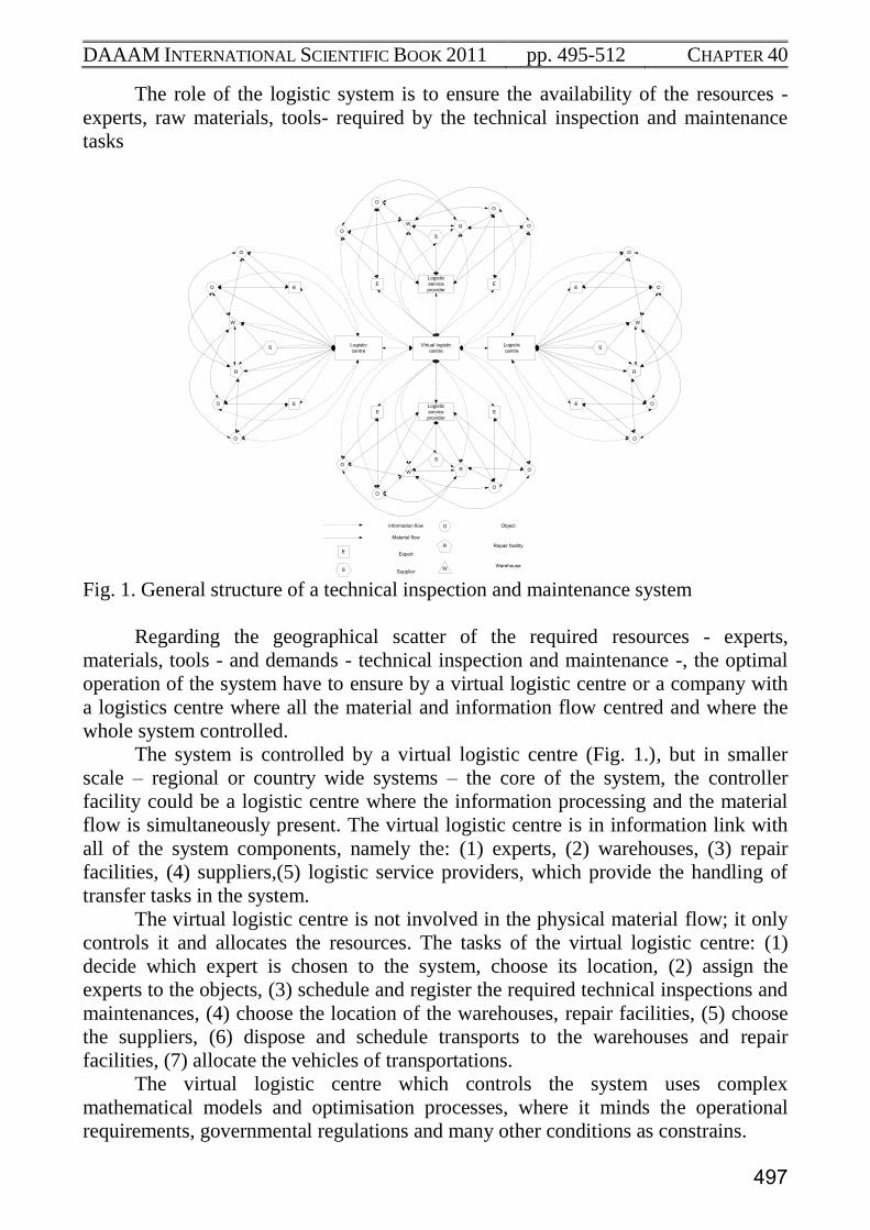
The role of the logistic system is to ensure the availability of the resources -

experts, raw materials, tools- required by the technical inspection and maintenance

tasks

Virtual logistic

centre

E

O

WR

O

O

Logistic

service

provider

E

O

Information flow

Material flow

EExpert

O Object

R

W

Repair facility

WarehouseS Supplier

S

E

O

WR

O

O

Logistic

service

provider

E

O

S

Logistic

centre

EO

W

R

O

O

E

O

SLogistic

centre

E

O

W

R

O

O

E

O

S

Fig. 1. General structure of a technical inspection and maintenance system

Regarding the geographical scatter of the required resources - experts,

materials, tools - and demands - technical inspection and maintenance -, the optimal

operation of the system have to ensure by a virtual logistic centre or a company with

a logistics centre where all the material and information flow centred and where the

whole system controlled.

The system is controlled by a virtual logistic centre (Fig. 1.), but in smaller

scale – regional or country wide systems – the core of the system, the controller

facility could be a logistic centre where the information processing and the material

flow is simultaneously present. The virtual logistic centre is in information link with

all of the system components, namely the: (1) experts, (2) warehouses, (3) repair

facilities, (4) suppliers,(5) logistic service providers, which provide the handling of

transfer tasks in the system.

The virtual logistic centre is not involved in the physical material flow; it only

controls it and allocates the resources. The tasks of the virtual logistic centre: (1)

decide which expert is chosen to the system, choose its location, (2) assign the

experts to the objects, (3) schedule and register the required technical inspections and

maintenances, (4) choose the location of the warehouses, repair facilities, (5) choose

the suppliers, (6) dispose and schedule transports to the warehouses and repair

facilities, (7) allocate the vehicles of transportations.

The virtual logistic centre which controls the system uses complex

mathematical models and optimisation processes, where it minds the operational

requirements, governmental regulations and many other conditions as constrains.

497


3. System components and their functions

3.1 Objects

The objects are such machines facilities which: (1) require – where p

is the number of the objects – maintenances in a time period, depends on the age or

technical condition or other regulations. (2)The inspections can be done with an

optional interval but it can’t be too short. (3) At all of the objects all the maintenances

are mandatory, in some cases it is defined by law.

3.2 Experts

In most cases they are specialized technical experts, who do the technical

inspections in the given period. Their role could be according to the type of the

system: (1) only technical inspection, supervision or control test, (2) do some smaller

maintenance tasks, (3) control and supervise and approve bigger maintenance tasks.

3.3 Repair facilities

Most of the inspection and maintenance tasks are performed onsite by the

experts occasionally with technicians of the repair company. In the repair facilities

such tasks are performed which cannot do onsite. The need of a repair facility

primarily appears at repairing large parts, or complex and long period repair tasks.

The tasks of a repair facility: (1) repair of the supplied parts, (2) refurbish of the

supplied parts, (3) recycle of the supplied parts and sometimes, (4) sell of the

refurbished parts or machines. The repair facility did not do any transportation tasks.

All the transportation done by the logistic service provider, or sometimes the experts

can transport smaller parts, tools. At the design of complex machines one of the

design targets is the modularity, so the machines can be maintain and repair fast with

swapping the defective module with a new, and therefore the downtime decreased to

the minimum and the defective module could be repaired – which is a long task in

time - or recycled at the repair facility.

3.4 Warehouses

The role of the warehouses is storing: (1) the spare parts, (2) the refurbished

parts, (3) some transportation vehicles, (4) auxiliary materials, consumables, tools,

etc.

It is important to uphold such a stock level which minimizes the downtime

caused by the maintenance.

3.5 Suppliers

The role of the suppliers is: (1) deliver the spare parts to the warehouses, (2)

deliver the tools, consumables to the repair facilities, (3) and deliver the tools and

consumables to the warehouses.

In these systems the transportation could be the task of: (1) the supplier, (2) an

external forwarder company, (3) the logistic centre.

Selecting the suppliers belongs to the main tasks of the virtual logistic centre.

498


3.6 Logistics service providers

The tasks of the external logistics service providers are to fulfil the tasks of

transportation, storage, or other complex logistic operations like finishing.

Distinguishing by their activities there is: (1) logistic service company: it does only

transportation and storage tasks (2) logistic centre: it does complex logistic services

beside the basic operations the storage and transportation

The transportation tasks are: (1) transport spare parts and tools from the warehouses

to the objects, (2) if the suppliers does not transport the spare parts on their own,

transport the spare parts from the suppliers to the warehouses, (3) transport the

supplied material to the repair facilities if the suppliers does not do, (4) transport the

repaired and refurbished parts from the repair facilities to the warehouses.

If the logistic service providers do any storage tasks then the role of the

warehouses are also applied (chapter 3.4). The storing at the logistic service providers

does not exclude the usage of dedicated warehouses near the sites.

The logistic centre could do the transportation, storage or even local disposition

tasks performing complex logistic services. Deploy or involve a logistic centre into

the system generally happen on regional level, because their scope of services is so

extensive they can substitute warehouses and logistic service companies on regional

level or even can perform some disposition and management tasks of the virtual

logistic centre.

3.7 Virtual logistics centre

The virtual logistic centre is the core of system. The virtual logistic centre

manages the operation of the system and does the following tasks: (1) select and

allocate and assign the required logistic resources, (2) collect and process the data

which required to the selection and the assignment of the optimal network elements,

(3) operate the information system to which all the system elements linked, (4) define

the management structure of the system and operate the logistic system, (5) collect

and store the data generated by the logistic networks and its connected elements

which needs to the system benchmarks and performance management, (6) constantly

monitoring on the performance and decide which element can outsourced and

examine the possibilities of forming regional centres.

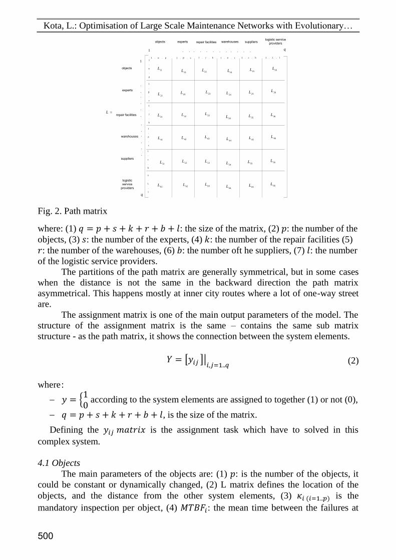
4. Mathematical model of the technical inspection and maintenance systems

The system main parameter is the path matrix, which shows the distance of the

system elements. In our case the path matrix is an integrated matrix, it builds up from

several sub matrixes, the sub matrix count defined by the number of elements in the

system.

(1)

499


L

1

1 q

.

.

.

.

.

.

.. .. ..

objects

experts

repair facilities

warehouses

objects experts repair facilities warehouses

11L

21L

21L 22

L

13L

14L

31L

41L

23L

24L

32L 33

L34

L

42L 43

L44

L

suppliers

51L 52

L53

L54

L

logistic

service

providers61

L 62L 63

L64

L

.. .. ..

logistic service

providers

15L

25L

35L

45L

55L

65L

suppliers

16L

26L

36L

46L

56L

66L

.

.

.

.

.

.

q

p

.

.

1

p..1 s..1 k..1 r..1 b..1 l..1

r

.

.

1

k

.

.

1

s

.

.

1

l

.

.

1

b

.

.

1

Fig. 2. Path matrix

where: (1) : the size of the matrix, (2) : the number of the

objects, (3) : the number of the experts, (4) : the number of the repair facilities (5)

: the number of the warehouses, (6) : the number oft he suppliers, (7) : the number

of the logistic service providers.

The partitions of the path matrix are generally symmetrical, but in some cases

when the distance is not the same in the backward direction the path matrix

asymmetrical. This happens mostly at inner city routes where a lot of one-way street

are.

The assignment matrix is one of the main output parameters of the model. The

structure of the assignment matrix is the same – contains the same sub matrix

structure - as the path matrix, it shows the connection between the system elements.

(2)

where :

according to the system elements are assigned to together (1) or not (0),

, is the size of the matrix.

Defining the is the assignment task which have to solved in this

complex system.

4.1 Objects

The main parameters of the objects are: (1) : is the number of the objects, it

could be constant or dynamically changed, (2) L matrix defines the location of the

objects, and the distance from the other system elements, (3) is the

mandatory inspection per object, (4) : the mean time between the failures at

500


the object i , from thos parameter one can calculate the required ad hoc

maintenance tasks, (5) is the average time of a technical inspection,

maintenance on the object i.

; (3)

The number of the technical inspections and maintenances could be prescribed

by law, governmental regulations in some cases where human life is endangered, like

the elevators. The maintenances can’t happen in a arbitrary period, there is a time

period which have to be defined to every object when the next maintenance task

couldn’t performed and the interval of the inspections fulfil the

;

(4)

constrain. In real conditions in these systems the inspection and maintenance tasks

are performed by the same expert so the special knowledge collected at the previous

inspections is well utilized so the maintenance times could be shortened.

4.2 Experts

The parameters for the mathematical description of the experts are the

following: (1) : is the number of the experts, constant in most cases, but it could

change for example at the case of: (a) expert leaving the job, (b) expert employment

in case of system expansion, (c) expert number decreasing in case of system

reduction it could be dynamic. (2) matrix: defines the location of the expert, well it

defines the distance of the experts from the other system elements, (3) : the average

speed of the expert, generally it defined as constant.

From these parameters the visiting time of the object i at the expert h can be

defined as:

(5)

where:

: is the distance between the object i and expert h.

The time required to travel between object i and j:

(6)

where: (1) : is the distance between the object i and j, (2) : is the performance of

the experts, it show how much maintenance task is performed by the expert.

Constrains:

The performance of the expert has to be between the defined minimum and

maximum values:

501


(7)

where

(8)

The cycle time ( ) - generally one day – is also a constraint, in one cycle the

expert visits the objects and return to his base location:

(9)

where: : is the interval when the expert start from his base location, visit the objects

and return, it is generally one day at the regional or countrywide maintenance

systems and:

(10)

where: (1) : is the number of cycles in the interval, (2) time interval of a

cycle, (3) : the number of object have to visit in the cycle t, (4)

: the travel time

to the first object, (5)

: the travel time from the last object to the experts base

location, (6) : the average inspection time of the object i.

The set of objects can be defined which have to inspect at the expert c:

; , (11)

and the subsets, the objects have to be inspected in one cycle:

, (12)

where: : is an ordered set, the objects assigned to the given expert, the ordering

function is:

, (13)

where: is the inspection time of , (2)

is the inspection time of ,

so the set is ordered by the visiting time.

, (14)

;

(15)

502


However the expert perform more than one inspection on an object so the

object is counted in the sets defined at (12) as many as the number of inspection has

to be performed on it. To determine the interval of the inspections the following

distance functions can apply:

, (16)

so based on the constrain (4):

. (17)

So the path travelled by the expert i in a cycle t can be describe as:

(18)

and the total path travelled by the expert p can be described as:

(19)

The expenditures (C) of the experts (S) in a given period (T) can described as:

(20)

where: (1) : is the specific cost for one kilometre, (2) : the specific cost for an

object. The main target function is the minimal expenditures:

. (21)

Unfortunately due to the limitation of this publication the whole model can’t be

presented here, but it is described in (Kota et al., 2002) but it has no impact on the

optimisation process described in the next chapter.

5. Literature on the multi-depot multiple travelling salesman problem

The problem area of the technical inspection and maintenance systems

discussed here is closest to the multiple travelling salesman problems (MTSP). And

within the MTSP it is the fixed destination multiple depot multiple travelling

salesman problem (MDMTSP), but the solutions in the literature did not mention the

additional sub tour construction. This area is poorly researched compared to the

general TSP or MTSP problems. Only the newest researches dealing with this field,

and they utilize such heuristic techniques as:

503


agent based modelling with probability collectives: (Anand et al., 2010)

developed a multi-agent model to solve the MTSP problem where they used

collective memory, probability collectives, and stochastic methods, the

algorithm use simple inserting, swap and elimination heuristics. They test the

algorithm in two simple cases with fifteen nodes and three agents,

genetic algorithm: (Suk-Tae Bae et al., 2007): They solve the problem with a

two phase algorithm. In the first phase the problem was reduced from a multi

centre problem into more single centre problems. In the second phase the

problems solved individually with a genetic algorithm. The algorithm was

tested up to 99 nodes and 4 agents,

ant colony algorithm, (Ghafurian et al., 2011): They used the ant colony

algorithm developed by Marco Dorigo (Dorigo, 2004) which is a well-

researched algorithm in these days (Crawford et al., 2009) and solve the

general MmTSP model, where artificial ants search the solution in a problem

tree modelled the foraging behaviour of real ants. The algorithm is compared

by the solution of the Lingo 8 software and it can be seen that the ant colony

heuristic algorithm is far faster and sometimes gives better solution. But the

algorithm was tested only up to 40 nodes and 5 agents.

The studies of optimisation of complex logistics systems can be categorized

into two main streams. The first stream addressed the application of meta-heuristic

optimisation and the second stream focuses on the application of simulation.

However simulation is a useful tool to optimise systems (Bányai, 2009), but the

complexity of the system can extremely increase the required execution time,

especially in the case of global, virtual systems (Bányai, 1999).

It can be seen that the developed methods was tested only a few nodes and they

not includes the special constrains what emerge in technical inspection and

maintenance system. But in the field of logistic there are systems with over 1000

nodes or rarely but systems with over 10000 nodes exist.

6. Optimisation of the complex expert object assignment of a technical

inspection and maintenance system with evolutionary programming

6.1 Evolutionary programming

The problem-solving algorithms, which are a known mechanism of evolution

are based on evolutionary algorithms are called. The most known algorithms are the:

(1) genetic algorithm, (2) evolutionary programming, (3) evolution strategic, (4)

neuro-evolution.

All the algorithms have a common part: they handle a population. The

population is consisting of individuals. One individual is one possible solution to the

problem. The target is to get the best solution to the given problem. But in the most of

the problems the algorithms didn’t have a chance the find the optimal solution and

the one have to satisfy with a quasi-optimal or a “good enough” solution.

The evolutionary programming is mainly used on heavily constrained

problems. This method is also handling a population but there are no limitations to

the problem representation like at the genetic algorithm where bit vectors describe the

504


individuals. Here the problems described as the problem allow, or it is the best for

computer algorithms. The pseudo code of the evolutionary programming is the

following:

1. generate the first population, in most cases it is random generated,

2. calculate the population fitness value

3. while not done

3.1. copy the population into a temporary population

3.2. run the mutation operators on the temporary population

3.3. select the survivors for the next population

4. end while

In the computer solutions first initialise the data, random generator, etc. Then

initialise the first population. In heavily constrained problems there are two cases: (1)

the random generated population individuals’ are invalid: it violates the constrains,

(2) the individuals are correct: but this is a very rare case.

There are several methods to get valid individuals from simply dispose invalid

individuals to create special operators which retain the individual’s integrity. But the

simplest solution is using penalty functions. In the penalty functions one can regulate

the algorithm which solutions are preferable.

After the creation of the initial population it have to copied into a temporary

population then the mutation operators run on the temporary population. In most

cases the high impact mutations have a lesser chance to run and the low impact

operators have a bigger chance. After the mutation we have to compute the mutated

individuals’ fitness value and then choose the survivor individuals to the descendant

population which happen with a championship. One simple way to perform the

championship is choose two random individuals one from the original and one from

the mutated population and that will survive which has a lesser (or bigger if the

fitness not normalized) fitness value, we have to repeat this until the new population

not filled.

At the evolutionary programming the vast majority of the cases there are no

crossover. In some solutions there is no meaning of this, and mostly it creates invalid

individuals. So in the biological view this is not an evolution of one species but the

evolution of many so calling it “population” is not valid but for the integrity of

evolutionary method this naming convention is common.

6.2 The problem representation in the proposed evolutionary programming algorithm

The developed algorithm solve the fixed destination multiple depot multiple

travelling salesman problem with sub tours and optimise the salesman count in one

phase and can be used on large or very large problems. As there are multiple

salesman: the experts, multiple depot: all the experts have different locations, fixed

destination: all the expert start and return to their initial location, and all the experts

do the travel in (generally) one day cycles. And crowns all it regards

The developed solution method based on a multi chromosome technique which

is not widely used in genetic algorithm but it could simply implement in the

evolutionary programming.

505


The data structure of the optimisation is built as describe in the 4.1. The biggest

container is the population which consists of defined constant number of individuals,

which is an input parameter of the optimisation

Population

Individual n

Expert n

Maint. 1 Maint. n

Fig. 3. The cascaded data structure of the optimisation

First the algorithm initializes the optimisation constants, like penalty constants,

maximum tour length, maximum cycle count, expert performance values and number

of the individuals in a population, load the data files of the experts, that’s define the

number of the experts and their location the objects which define the number of the

objects and its location, and initialize maintenances data. Then it creates the first

population with random generated individuals. It is a top down algorithm: (1) first

generate individuals container, (2) then generate experts container and insert it into

the individuals, (3) then generate chromosome and insert it into the experts so that fill

the chromosome with maintenances in a random generated order. So every expert is a

chromosome that’s why the algorithm named as multi chromosome algorithm. Then

it calculates the fitness values of the experts and applies the penalty functions for the

experts, finally apply the global penalty functions for the individual.

6.3 Penalty functions

The penalty functions is one of the simplest and fastest way to rate the

individual, so the goodness of the actual solution. In this algorithm there are (1) local

- the penalty function is applied to the expert – and (2) global - the penalty function is

applied to the whole individual -

penalty functions applied.

6.3.1 Local penalties

There are four different local penalty functions:

Cycle count penalty: when the expert do more route cycles as the

allowed(5),

Few penalty : the expert has to get a minimal number of maintenances (8),

More penalty: the expert cannot get more maintenances than his maximum

capacity (8),

Near penalty: the maintenances of one object cannot be arbitrarily close (4).

Cycle count penalty function of the expert i:

(22)

506


where:

: constant, the penalty value of the cycle count violation

: the actual number of the expert’s cycles.

Few penalty function of the expert i:

(23)

where:

: constant, the penalty value of the few maintenances violation

: the actual performance of the expert i, the number of the maintenances

The more penalty function of the expert i:

(24)

where: (1) : constant, the penalty value of the more maintenances violation (2) :

the actual performance of the expert i, the number of the maintenances

The near penalty function is the following:

+1;

(25)

where: (1) : the maintenance i of the object x, (2) : constant, the penalty value

of the near maintenances violation, (3) : indexof operator, show the index of the

given maintenance, (4) : the number of the maintenance near violations.

6.3.2 Global penalties

There are two different global penalty functions, which calculated after the

local penalties: (1) Scatter penalty: which applied when an object’s maintenances are

scattered among several experts (chapter 4.2), (2) Expert count penalty: The expert’s

employment have a fixed cost in this model. Due to this penalty functions the

algorithm try to minimize the number of employed experts.

Scatter penalty function is the following:

(26)

where: (1) : is the count of the maintenances of the object i at the expert x

(2) : the required maintenances of the object I (3) : constant, the

penalty value of scattered maintenances.

507


Expert count penalty function:

s (27)

where: (1) : constant, the cost of one experts’ employment, (2) : the number of

the experts.

Then the algorithm enters into the optimisations’ main loop (chapter 6.1) and

copies the population individuals into a temporary population in order of their fitness

so the best fitness value individual is copied into the first position of the temporary

population. The applied operators in the algorithm are simple and more or less

common at the genetic methods, because more the operators are simpler the faster the

algorithm.

6.4 Mutation operators

In the mutation phase the algorithm mutates the individuals in the temporary

population. There are two types of mutation operators due to the multi chromosome

characteristic: (1) inner expert mutation operators and (2) cross expert mutation

operators.

6.4.1 Inner expert mutation

There are three types of inner expert mutation operators:

Gene swap: where two random genes are swapped:

O3M1 O2M1 O3M2 O1M2 O3M3 O2M2Expert n Fig. 4. Gene swap operator

Gene sequence reversion: where the gene sequence are reversed between two

random indexes

O3M1 O2M1 O3M2 O1M2 O3M3 O2M2Expert n Fig. 5. Gene reversion operator

Gene insertion operator: where a randomly chosen gene inserted into a

randomly chosen position

O3M1 O2M1 O3M2 O1M2 O3M3 O2M2

O3M1 O2M1O3M2 O1M2 O3M3 O2M2 Fig. 6. Gene insertion

508


6.4.2 Cross expert mutation Like the inner expert mutation operators there are also three types of mutation operators exists for the cross expert mutation. These are the followings:

Cross expert gene swap: which swaps two genes between experts. The second expert and the position of the second gene are chosen randomly.

O3M1 O2M1 O3M2 O1M2 O3M3 O2M2Expert n

O1M1 O2M4O1M3 O2M3 O3M4 O1M4Expert m Fig. 7. Cross expert gene swap

Cross expert gene sequence change: where the algorithm swapping a randomly chosen but continuous gene sequence with a randomly chosen expert also randomly chosen gene sequence:


O1M1 O2M4O1M3 O2M3 O3M4 O1M4Expert m

O3M1

O2M1 O3M2

O1M2 O3M3 O2M2Expert n

O1M1

O2M4

O1M3

O2M3 O3M4

O1M4Expert m Fig. 8. Cross expert gene sequence swap

Cross expert gene contraction: where random amount of genes inserted to a randomly chosen expert from the end of the chromosome


O1M1 O2M4O1M3 O2M3 O3M4 O1M4Expert m

O3M1 O2M1 O3M2

O1M2 O3M3 O2M2

Expert n

O1M1 O2M4O1M3 O2M3 O3M4 O1M4Expert m Fig. 9. Cross expert chromosome contraction The mutations are chosen randomly for every expert with parameterised probability and the algorithm allows a probabilistic value for the no mutation also. 6.5 Survivor selection

First the algorithm search for the best individual and copy it to the descendant population. Its called elitism, the best individual (elitist) always survives. The evolutionary programming typically uses stochastic tournament survivor selection. The simplest of the tournament selection is when randomly choose two individuals, one from the original and one from the mutated population and the fittest win, that individual will be copied into the next generation of the individual. This process is repeated until the next population is filled.

509


But for avoiding the local optimums all of the genetic methods trying to maintain the diversity among the individuals, in this algorithm one can parameterise how much individual in the descendant population will be filled with random generated individuals

The main loop of the optimisation now stops on an exact repetition count.

7. Results The algorithm was tested on several tsp files from the de facto standard

TSPLIB sample instances with random experts’ locations. The algorithm gives very good run times on large (1000 – 2000 objects and 30-50 experts) instances. It is tested on a very large instance over 11000 objects but the running time with the current implementation is a bit long, about 2-3 weeks on a 2.9Ghz I7 machine using a single core. Convergence with the tsplib att48.tsp file: file: tsplib att48 running time: 20 sec

objects: 48; experts: 5 population size 100; iterations 1000

Tab 1. tsplib att48

As the diagram shows, the algorithm convergences very fast in this simple instance, at the first 100 iterations and after then get slower up to the 400 iteration at this simple instance and then no further improvements are visible. But this is usual in the field of genetic methods Convergence with the tsplib pr654 file:

file: tsplib pr654 running time: 29 min 30 sec

objects: 654; experts: 30 population size 100; iterations 1500

Tab. 2. tsplib pr654

510


At this instance the diagram shows very fast convergence up to 600 iterations

and after then only minor improvement happened. This instance with the 654 nodes

counts a medium size instance in the field of logistics.

Convergence with the tsplib pr1002file:

file: tsplib pr1002

running time: 3 hours 55 min 15 sec

objects: 1002; experts: 30

population size 100; iterations 5000

Tab 3. tsplib pr1002

At this large instance the convergence a bit worse than the previous instances.

As it can be seen the target function improves fast up to the 2000 iteration count and

after that only minor improvements can be observed.

As it can be seen that, the execution time is increasing as the problem size

grows, but it is stay in manageable range even in this large problem size. But a little

over this size the further improvement of the implementation of the algorithm

requires parallelization or other performance increase method.

8. Further researches

The optimisation method has great potentials toward the further improvements.

First some improvement in the method himself:

try new mutation methods,

try new survivor tournament selection methods.

Second some improvements which have a great impact on speed:

parallelization: some current researches which is not ready for publications a

simple parallelization of fitness calculation can improve the running time by

reducing it to the third in large scale problems, but in small scale the task

switching and data moving processes slower the calculation.

examine the implementation possibilities on a fast graphics processing unit.

9. Acknowledgements

The research was supported by the TÁMOP 4.2.1.B-10/2/KONV entitled

Increasing the quality of higher education through the development of research -

development and innovation program at the University of Miskolc.

511


10. References

Anand J. Kulkarni, K. Tai (2010): Probability Collectives: A multi-agent approach

for solving combinatorial optimization problems, Applied Soft Computing 10,

pp.: 759–771, doi:10.1016/j.asoc.2009.09.006

Bányai, Á. (1999) Das virtuelle Logistikzentrum als Koordinator der logistischen

Aufgaben. In: Modelling and optimization of logistic systems – Theory and

practice, Bányai, T. & Cselényi, J. (Eds.), pp. 42-50, ISBN 963 661 402 4,

Published by the University Miskolc

Bányai, T. (2009): Optimisation of U-shaped flexible manufacturing cells. In: Annals

of DAAAM for 2009 & Proceedings of the 20th International DAAAM

Symposium "Intelligent Manufacturing & Automation: Focus on Theory,

Practice and Education", Katalinic, B. (Ed.), pp. 761-762, ISSN 1726-9679,

ISBN 978-3-901509-70-4, Vienna, Austria, November 2009, Published by

DAAAM International Vienna

Crawford, B.; Castro, C. & Monfroy, E. (2009): Enhancing the Transition Rule in

Ant Computing for the Set Covering Problem, Annals of DAAAM for 2009 &

Proceedings of the 20th International DAAAM Symposium, 25-28th November

2009, Vienna, Austria, ISSN 1726-9679, ISBN 978-3-901509-70-4, Katalinic,

B. (Ed.), pp. 1329-1330, Published by DAAAM International Vienna, Vienna

Dorigo, M., Stützle T. (2004): Ant Colony Optimization, MIT Press. ISBN 0-262-

04219-3

Kota, L., Cselényi, J. (2002): Defining the new experts location in an elevator

maintenance examination system, “Вестник Национального технического

Университета «ХПИ» 9’2002 т. 10, Харьков, Сборник научных трудов

Тематический выпуск” “Технологии в машиностроении“ Удк 621.9,

страницы:96-102

Ghafurian, S., Javadian, N. (2011): An ant colony algorithm for solving fixed

destination multi-depot multiple traveling salesmen problems, Applied Soft

Computing 11, pp.: 1256–1262

Suk-Tae, B., Heung Suk, H., Gyu-Sung, C. and Meng-Jong G. (2007): Integrated

GA-VRP solver for multi-depot system, Computers & Industrial Engineering

Volume 53, Issue 2, Pages 233-240, doi:10.1016/j.cie.2007.06.014

512

o large scale maintenance n evolutionary …

Documents