o n the use of numeraires in o ption...

O n the Use of Numeraires in O ption Pricing

Simon B enninga¤

F a c ulty o f M a na g e me nt

T e l-A v iv U niv e rsity ISRA EL

U niv e rsity o f Gro ning e n H OLLA N D

e -ma il: be nning a @po st.ta u.a c .il

T omas B jÄor kD e pa rtme nt o f F ina nc e

Sto c k ho lm Sc ho o l o f Ec o no mic s

SWED EN

e -ma il: ¯[email protected]

Zvi Wiener y

Sc ho o l o f Busine ss

H e bre w U niv e rsity o f Je rusa le m

ISRA EL

e -ma il: msw ie ne r@msc c .huji.a c .il

Oc t o b e r , 2 0 0 2

Forthcoming in The Journal of Derivatives

¤ B en n in ga ack n ow led ges a gr an t fr om th e Isr ael In stitu te of B u sin ess Resear ch at T el-A v ivU n iv er sity .

y W ien er 's r esear ch w as fu n d ed b y th e Kr u eger C en ter at th e H eb r ew U n iv er sity .

1

On t h e U s e o f N u m e r a ir e s in Op t io n P r ic in g

A b s t ra ct

In this pa pe r w e disc uss the sig ni c a nt c o mputa tio na l simpli c a tio ntha t o c c urs w he n o ptio n pric ing is a ppro a c he d thro ug h the c ha ng e o fnume ra ire te c hniq ue . By pric ing a n a sse t in te rms o f a no the r tra de d a s-se t (the nume ra ire ), this te c hniq ue re duc e s the numbe r o f so urc e s o f riskw hic h ne e d to be a c c o unte d fo r. Orig ina lly de v e lo pe d by Ge ma n (1 9 8 9 )a nd Ja mshidia n (1 9 8 9 ), this te c hniq ue is use ful in pric ing c o mplic a te dde riv a tiv e s. In this pa pe r w e disc uss the unde rly ing the o ry o f the nu-me ra ire te c hniq ue , a nd illustra te it w ith ¯v e pric ing pro ble ms:

² Pric ing sa v ing s pla ns w hic h inc o rpo ra te a c ho ic e o f link a g e .

² Pric ing c o nv e rtible bo nds.

² Pric ing e mplo y e e sto c k o w ne rship pla ns

² Pric ing o ptio ns w he re the strik e pric e is in a c urre nc y di®e re nt fro mthe sto c k pric e .

² Pric ing o ptio ns w he re the strik e pric e is c o rre la te d w ith the sho rt-te rm inte re st ra te

JEL classi¯cation: G12, G13

2

Contents

1 Introduction 4

2 The change of numeraire approach 5

3 Employee stock ownership plans 8

3.1 Institutional setup . . . . . . . . . . . . . . . . . . . . . . . . . . 8

3.2 Mathematical model . . . . . . . . . . . . . . . . . . . . . . . . . 8

4 Options with a foreign-currency strike price 11



4.3 Pricing the option in dollars . . . . . . . . . . . . . . . . . . . . . 13

4.4 Pricing the option directly in pounds . . . . . . . . . . . . . . . . 14

5 Pricing convertible bonds 16



6 Pricing savings plans with choice of linkage 19



7 Endowment warrants 21



8 Conclusion 26

3

1 I ntr oduction

In this paper we explore ¯ve applications of the numeraire method in option pric-ing. While the numeraire method is well-known in the theoretical literature, itappears to be infrequently used in more applied papers, and many practitionersseem to be unaware of how to use it as well as when it is pro¯table (or not) touse it. In order to illustrate the uses (and possible misuses) of the method wediscuss in some detail ¯ve concrete applied problems in option pricing:

² Pricing savings plans which incorporate a choice of linkage.

² Pricing convertible bonds.

² Pricing employee stock ownership plans

² Pricing options where the strike price is in a currency di®erent from thestock price.

² Pricing options where the strike price is correlated with the short-terminterest rate

The standard Black-Scholes (BS) formula prices a European option on an assetthat follows a geometric Brownian motion. The asset's uncertainty is the onlyrisk factor in the model. A more general approach developed by Black-Merton-Scholes leads to a partial di®erential equation. The most general method de-veloped so far for the pricing of contingent claims is the martingale approachto arbitrage thory developed by Harrison-Kreps (1981), Harrison-Pliska (1981)and others. However, whether one uses the PDE or the standard \risk neutralvaluation" formulas of the martingale method, it is in most cases very hard toobtain analytic pricing formulas. Thus, for many important cases, special for-mulas (typically modi¯cations of the original BS formula), were developed. SeeHaug (1997) for an extensive set of examples.

One of the most typical cases of several risk factors occurs when an option isto choose among two assets with stochastic prices. In such a case it is oftenof considerable advantage to use a change of numeraire in the pricing of theoption. In what follows we demonstrate examples where the numeraire approachleads to signi¯cant simpli¯cations but, in order not to oversell the method, alsoexamples where the numeraire change is trivial or where an obvious numerairechange really does not simplify the computations. The main message is still thatin many cases the change of numeraire approach leads to a drastic simpli¯cationof the computational work.

In section 2 we start with a brief introductory review of the numeraire method,followed by a mathematical summary (which can be skipped on ¯rst readingof this paper). In sections 7-4 we then present ¯ve di®erent option pricingproblems. For each problem we present the possible choices of numeraire, discussthe pros and cons of the various numeraires, and compute the option prices.

4

2 T he change of numer air e appr oach

The basic idea of the numeraire approach can be described as follows: Supposethat an option's price depends on several (say n) sources of risk. We may thencompute the price of the option according to the following scheme:

² Fix a security which embodies one of the sources of risk, and choose thissecurity as the numeraire.

² Express all prices on the market, including that of the option, in terms ofthe chosen numeraire. In other words, we perform all our computationsin a relative price system.

² Since the numeraire asset in the new price system is riskless (by de¯nition)we have decreased the number of risk factors by one from n to n¡1. If, forexample, we started out with two sources of risk, we can now often applystandard one-risk-factor option pricing formulas (such as Black-Scholes).

² We thus derive the option price in terms of the numeraire. A simpletranslation from the numeraire back to the local currency will then givethe price of the option in monetary terms.

These ideas were developed independently by Geman (1989) and Jamshidian(1989).1 The standard reference in an abstract setting is Geman, et.al. (1995).In the remainder of this section, we consider a Markovian framework which issimpler than that of the last paper, but which is still reasonably general. Alldetails and proofs can be found in BjÄork (1999).2

Assumption 2.1 The following objects are given a priori.

² An empirically observable (k + 1)-dimensional stochastic process

X = (X1; : : : ;Xk + 1);

with the notational convention

Xk + 1(t) = r(t):

² We assume that under a ¯xed risk neutral martingale measure Q, thefactor dynamics have the form

dXi(t) = ¹i (t;X(t)) dt + ±i (t; X(t)) dW (t); i = 1; : : : ; k + 1;

where W = (W1; : : : ; Wd)0 is a standard d-dimensional Q-Wiener process.The superscript 0 denotes transpose.

1 T h e ear liest in car n ation of a sim ilar id ea is to b e fou n d in p ap er s b y Fisch er (1978) an dB r en n er an d Galai (1978).

2 T h e r em ain d er of th is section can b e sk ip p ed b y r ead er s in ter ested on ly in th e im p lem en -tation of th e n u m er air e m eth od .

5

² A risk free asset (money account) with the dynamics

dB(t) = r(t)B(t)dt:

The interpetation of this is that the components of the vector process X are theunderlying factors in the economy. We make no a priori market assumptions,so whether or not a particular component is the price process of a traded assetin the market will depend on the particular application. We now also introduceasset prices, driven by the underlying factors, in the economy.

Assumption 2.2

² We consider a ¯xed set of price processes S0(t); : : : ; Sn(t), each of which isassumed to be the arbitrage free price process for some traded asset withoutdividends.

² Under the risk neutral measure Q, the S-dynamics have the form

dSi(t) = r(t)Si(t)dt + Si(t)dX

j = 1

¾ij(t; X(t))dWj(t); (1)

for i = 0; : : : ; n ¡ 1.

² The nth asset price is always given by

Sn(t) = B(t);

and thus (1) also holds for i = n with ¾nj = 0 for j = 1; : : : ; d:

We now ¯x an arbitary asset as the numeraire, and for notational conveni-nence we assume that it is S0. We may then express all other asset pricesin terms of the numeraire S0, thus obtaining the normalized price vectorZ = (Z0; Z1; : : : ; Zn), de¯ned by

Zi(t) =Si(t)

S0(t):

We now have two formal economies: the S economy where prices are measuredin he local currency (such as dollars), and the Z-economy, where prices aremeasured in terms of the numeraire S0.

The main result is the following theorem, which shows how to price an arbitrarycontingent claim in terms of the chosen numeraire. For brevity, a contingentclaim with exercise date T will henceforth be referred to as a \T -claim".

Theorem 2.1 (Main theorem) Let the numeraire S0 be the price process fora traded assset with S0(t) > 0 for all t. Then there exists a probability measure,denoted by Q0, with the following properties.

6

² For every T -claim Y , the corresponding arbitrage free price process ¦(t;Y )in the S-economy is given by

¦(t;Y ) = S0(t)¦Z

µt;

Y

S0(T )

¶; (2)

where ¦Z denotes the arbitrage free price in the Z-economy.

² For any T -claim ~Y , its arbitrage free price process ¦Z in the Z economyis given by the formula

¦Z³t; ~Y

´= E0

t;X(t)

h~Yi; (3)

where E0 denotes expectation w.r.t. Q0. In particular, the pricing formula(2) can be written

¦(t; Y ) = S0(t)E0t;X(t)

·Y

S0(T )

¸: (4)

² The Q0-dynamics of the Z-processes are given by

dZi = Zi [¾i ¡ ¾0] dW0; i = 0; : : : ; n: (5)

² The Q0-dynamics of the price processes are given by

dSi = Si (r + ¾i¾00) dt + Si¾idW 0; (6)

where W 0 is a Q0-Wiener process.

² The Q0-dynamics of the X-processes are given by

dXi = (¹i + ±i¾00) dt + ±idW 0: (7)

² The measure Q0 depends upon the choice of numeraire asset S0, but thesame measure is used for all claims, regardless of their exercise dates.

In passing we note that if we use the money account B as the numeraire, then thepricing formula above reduces to the well known standard risk neutral valuationformula

¦ (t;Y ) = B(t)E0t;X(t)

·Y

B(T )

¸= E0

t;X(t)

·e¡

R T

tr(s)ds

Y

¸(8)

In more pedestrian terms, the main points of the Theorem above are as follows.

² The pricing formula (2) shows that the measure Q0 \takes care of thestochasticity" related to the numeraire S0. Note that we do not have tocompute the price S0(t){we simply use the observed market price. We

7

also see that if the claim Y is of the form Y = Y0 ¢ S0(T ) (where Y0

is some T -claim) then the change of numeraire is a huge simpli¯cationof the standard risk neutral formula (8): Instead of computing the joint

distribution ofR T

t r(s)ds and Y (under Q) we only have to compute thedistribution of Y0 (under Q0).

² The formula (3) shows that in the Z economy, prices are computed asexpected values of the claim. Observe that there is no discounting factorin (3). The reason for this is that in the Z economy, the price process Z0

has the property that Z0(t) = 1 for all t. Thus, in the Z-economy there isa riskless asset with unit price, i.e. in the Z economy the short rateequals zero.

² Formula (5) says that the normalized price processes are martingales (i.e.zero drift) under Q0, and identi¯es the relevant volatility.

² Formulas (6)-(7) shows how the dynamics of the asset prices and the un-derlying a factors change when we move from Q to Q0. Note that thecrucial object is the volatility ¾0 if the numeraire asset.

In the following sections we show examples of the use of the numeraire methodwhich illustrate the considerable conceptual and implementational simpli¯cationto which this method leads.

3 E mployee stock owner ship plans

3.1 I nstitutional setup

In employee stock ownership plans (ESOP) it is common to include an optionof essentially the following form: The holder has the right to buy a stock at theminimum between its price in 6 months and in 1 year minus a rebate (say 15%).The exercise is one year.

3.2 M athematical model

In a more general setting the ESOP is a contingent claim Y , to be paid out attime T1, of the form

Y = S(T )¡ ¯ min [S(T1); S(T0)] ; (9)

so in the concrete case above we would have ¯ = 0:85, T0 = 1=2 and T1 = 1.The problem is to price Y at some time t · T0, and to this end we assume astandard Black-Scholes model where, under the usual risk neutral measure Qwe have the dynamics

dS(t) = rS(t)dt + ¾S(t)dW (t); (10)

dB(t) = rB(t)dt; (11)

8

with a deterministic and constant short rate r. The price ¦ (t;Y ) of the optioncan obviously be written

¦ (t; Y ) = S(t)¡ ¯¦(t; Y0)

where the T1-claim Y0 is de¯ned by

Y0 = min [S(T1); S(T0)] :

In order to compute the price of Y0 we now basically want to do as follows.

² Perform a suitable change of numeraire.

² Use a standard version of some well known option pricing formula.

The problem with carrying out this small program is that, at the exercise timeT1, the term S(T0) does not have a natural interpretation as a spot price of atraded asset. In order to overcome this di±culty we therefore introduce a newasset S0 de¯ned by

S0(t) =

½S(t); 0 · t · T0;

S(T0)er(t¡T0); T0 · t · T1:

In other words, S0 can be thought of as the value of a self ¯nancing portfoliowhere you at t = 0 buy one share of the underlying stock and keep it untilt = T0. At t = T0 you then sell the share and put all the money into the bankaccount.

We then have S0(T1) = S(T0)er(T1¡T0) so we can now express Y0 in terms ofS0(T1) as

Y0 = min [S(T1); K ¢ S0(T1)] (12)

whereK = e¡r(T1¡T0) (13)

The point of this is that S0(T1) in (12) can formally be treated as the price atT1 of a traded asset. In fact, from the de¯nition above we have the followingtrivial Q-dynamics for S0

dS0(t) = rS0(t)dt + S0(t)¾0(t)dW (t)

where the deterministic volatility is de¯ned by

¾0(t) =

½¾; 0 · t · T0;0; T0 · t · T1:

(14)

It is now time to perform a change of numeraire, and we can choose either Sor S0 as the numeraire. From a logical point of view the choice is irrelevant,but the computations become somewhat easier if we choose S0. With S0 as the

9

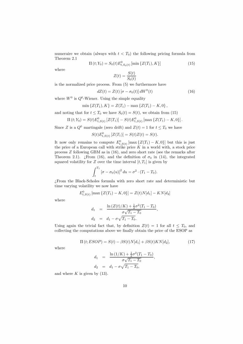
numeraire we obtain (always with t < T0) the following pricing formula fromTheorem 2.1

¦ (t;Y0) = S0(t)E0t;S0(t)

[min fZ(T1);Kg] (15)

where

Z(t) =S(t)

S0(t)

is the normalized price process. From (5) we furthermore have

dZ(t) = Z(t) [¾ ¡ ¾0(t)]dW 0(t) (16)

where W 0 is Q0-Wiener. Using the simple equality

min fZ(T1);Kg = Z(T1)¡ max fZ(T1)¡ K; 0g ;

and noting that for t · T0 we have S0(t) = S(t), we obtain from (15)

¦ (t; Y0) = S(t)E0t;S(t) [Z(T1)] ¡ S(t)E0

t;S(t) [max fZ(T1) ¡K; 0g] :Since Z is a Q0 martingale (zero drift) and Z(t) = 1 for t · T0 we have

S(t)E0t;S(t) [Z(T1)] = S(t)Z(t) = S(t):

It now only remains to compute E0t;S(t) [max fZ(T1)¡ K; 0g] but this is just

the price of a European call with strike price K in a world with, a stock priceprocess Z following GBM as in (16), and zero short rate (see the remarks afterTheorem 2.1). >From (16), and the de¯nition of ¾0 in (14), the integratedsquared volatility for Z over the time interval [t; T1] is given by

Z T1

t

[¾ ¡ ¾0(u)]2 du = ¾2 ¢ (T1 ¡ T0):

>From the Black-Scholes formula with zero short rate and deterministic buttime varying volatility we now have

E0t;S(t) [max fZ(T1) ¡K; 0g] = Z(t)N[d1] ¡KN [d2]

where

d1 =ln (Z(t)=K) + 1

2¾2(T1 ¡ T0)

¾p

T1 ¡ T0

;

d2 = d1 ¡ ¾p

T1 ¡ T0:

Using again the trivial fact that, by de¯nition Z(t) = 1 for all t · T0, andcollecting the computations above we ¯nally obtain the price of the ESOP as

¦ (t;ESOP ) = S(t)¡ ¯S(t)N[d1] + ¯S(t)KN [d2]; (17)

where

d1 =ln (1=K) + 1

2¾2(T1 ¡ T0)

¾p

T1 ¡ T0

;

d2 = d1 ¡ ¾p

T1 ¡ T0;

and where K is given by (13).

10

4 Options with a for eign-cur r ency str ike pr ice

In this section we discuss options whose strike price is linked to a non-domesticcurrency. We illustrate with the example of an option with a US dollar strikeprice on a stock denominated in UK pounds. Such options might be part ofan executive compensation program; such options might be given to motivatemanagers to maximize the dollar price of their stock. Another example is anoption where the strike price is CPI-indexed.


For purposes of illustration we assume that the underlying security is traded inthe UK in pound sterling and that the option exercise price is in dollars. Theinstitutional setup is as follows.

² The option is initially (i.e. at t = 0) an at-the-money option, when thestrike price is expressed in pounds.3

² This pound strike price is, at t = 0, converted into dollars.

² The dollar strike price thus computed is kept constant during the life ofthe option.

² At the exercise date t = T the holder can pay the ¯xed dollar strike pricein order to obtain the underlying stock.

² The option is fully dividend protected.

Since the stock is traded in pounds, the ¯xed dollar strike corresponds to arandomly changing strike price when expressed in pounds; thus we have a non-trivial valuation problem. The numeraire approach can be used to simplify thevaluation of such an option. The resulting valuation is given in (23).


We model the stock price S (in pounds) as a standard geometric Brownianmotion under the objective probability measure P , and we assume deterministicshort rates rp and rd in the UK and the US market respectively. Since we haveassumed complete dividend protection we may as well assume (from a formalpoint of view) that S is without dividends. We thus have the following P -dynamics for the stock price.

dS(t) = ®S(t)dt + S(t)±SdWS(t);

3For tax r eason s m ost ex ecu tiv e stock op tion s ar e in itially at-th e-m on ey .

11

We denote the dollar/pound exchange rate by X, and assume a standard Garman-Kohlhagen (1983) model for X. We thus have P -dynamics given by

dX(t) = ®XX(t)dt + X(t)±XdWX(t);

Denoting the pound/dollar exchange rate by Y , where Y = 1=X, we immedi-ately have the dynamics

dY (t) = ®Y Y (t)dt + Y (t)±Y dWY (t)

where ®Y is of no interest for pricing purposes. Here WS , WX and WY arescalar Wiener processes and we have the relations

±Y = ±X (18)

WY = ¡WX ; (19)

dWS(t) ¢ dWX(t) = ½dt; (20)

dWS(t) ¢ dWY (t) = ¡½dt: (21)

For computational purposes it is sometimes convenient to express the dynamicsin terms of a two dimensional Wiener process W with independent componentsintead of using the two correlated processes WX and WS . Logically the twoapproaches are equivalent, and in the new W -formalism we then have the P -dynamics

dS(t) = ®S(t)dt + S(t)¾SdW (t);

dX(t) = ®XX(t)dt + X(t)¾XdW (t);

dY (t) = ®Y Y (t)dt + Y (t)¾Y dW (t):

The volatilities ¾S , ¾X and ¾Y are two-dimensional row vectors with the prop-erties that

¾Y = ¡¾X

k¾Xk2 = ±2X ;

k¾Y k2 = ±2Y ;

k¾Sk2 = ±2S ;

¾X¾0S = ½±X±S

¾Y ¾0S = ¡½±Y ±S

where 0 denotes transpose and k k denotes the Euclidian norm in R2.

The initial strike price expressed in pounds is by de¯nition given by

Kp(0) = S(0);

and the corresponding dollar strike price is thus

Kd = Kp(0) ¢ X(0) = S(0)X(0):

12

The dollar strike price is kept constant until the exercise date. However, ex-pressed in pounds the strike price evolves dynamically as a result of the varyingexchange rate, so the pound strike at maturity is given by

Kp(T ) = Kd ¢ X(T )¡1 = S(0) ¢ X(0) ¢X(T )¡1: (22)

There are now two natural ways to value this option: we can work in dollars orin pounds, and initially it is not obvious which way is the easier. We will in factperform the calculations in both alternatives and compare the computationale®ort. As will be seen below it turms out to be slightly easier to work in dollarsthan in pounds.

4.3 P r icing the option in dollar s

In this approach we transfer all data into dollars. The stock price, expressed indollars, is given by

Sd(t) = S(t) ¢X(t);

so in dollar terms the payout ©d of the option at maturity is given by theexpression

©d = max [S(T )X(T )¡Kd; 0]

Since the dollar strike Kd is constant we can use the Black-Scholes formulaapplied to the dollar price process Sd(t). The Ito formula applied to Sd(t) =S(t)X(t) immediately gives us the P -dynamics of Sd(t) as

dSd(t) = Sd(t) (® + ®X + ¾S¾0X) dt + Sd(t) (¾S + ¾X) dW (t)

We can write this as

dSd(t) = Sd(t) (® + ®X + ¾S¾0X) dt + Sd(t)±S;ddV (t)

where V is a scalar Wiener process and where

±S;d = k¾S + ¾Xk =q

±2S + ±2

X + 2½±S±X

is the dollar volatility of the stock price.

The dollar price (expressed in dollar data) at t of the option is now obtaineddirectly from the Black-Scholes formula as

Cd(t) = Sd(t)N [d1] ¡ e¡rd(T¡t)KdN [d2]; (23)

d1 =ln (Sd(t)=Kd) +

³rd + 1

2±2S;d

´(T ¡ t)

±S;d

pT ¡ t

;

d2 = d1 ¡ ±S;d

pT ¡ t:

The corresponding price in pound terms is ¯nally obtained as

Cp(t) = Cd(t) ¢ 1

X(t);

13

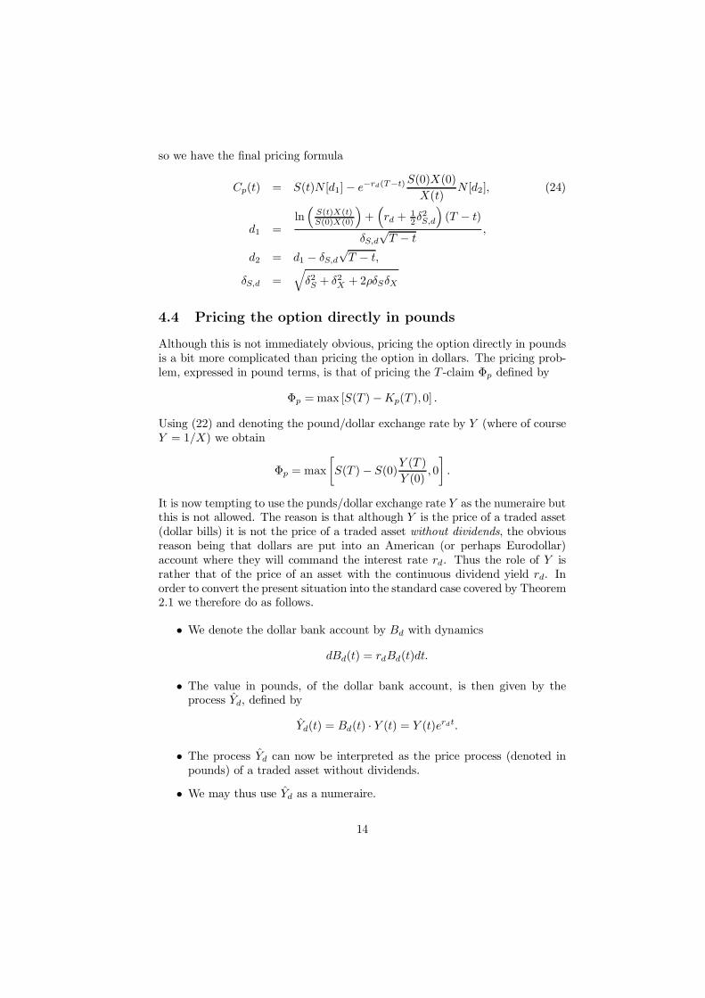
so we have the ¯nal pricing formula

Cp(t) = S(t)N [d1] ¡ e¡rd(T¡t) S(0)X(0)

X(t)N [d2]; (24)

d1 =ln

³S(t)X(t)S(0)X(0)

´+

³rd + 1

2±2S;d

´(T ¡ t)

±S;d

pT ¡ t

;

d2 = d1 ¡ ±S;d

pT ¡ t;

±S;d =q

±2S + ±2

X + 2½±S±X

4.4 P r icing the option dir ectly in pounds

Although this is not immediately obvious, pricing the option directly in poundsis a bit more complicated than pricing the option in dollars. The pricing prob-lem, expressed in pound terms, is that of pricing the T -claim ©p de¯ned by

©p = max [S(T ) ¡Kp(T ); 0] :

Using (22) and denoting the pound/dollar exchange rate by Y (where of courseY = 1=X) we obtain

©p = max

·S(T ) ¡ S(0)

Y (T )

Y (0); 0

¸:

It is now tempting to use the punds/dollar exchange rate Y as the numeraire butthis is not allowed. The reason is that although Y is the price of a traded asset(dollar bills) it is not the price of a traded asset without dividends, the obviousreason being that dollars are put into an American (or perhaps Eurodollar)account where they will command the interest rate rd. Thus the role of Y israther that of the price of an asset with the continuous dividend yield rd. Inorder to convert the present situation into the standard case covered by Theorem2.1 we therefore do as follows.

² We denote the dollar bank account by Bd with dynamics

dBd(t) = rdBd(t)dt:

² The value in pounds, of the dollar bank account, is then given by theprocess Yd, de¯ned by

Yd(t) = Bd(t) ¢ Y (t) = Y (t)erdt:

² The process Yd can now be interpreted as the price process (denoted inpounds) of a traded asset without dividends.

² We may thus use Yd as a numeraire.

14

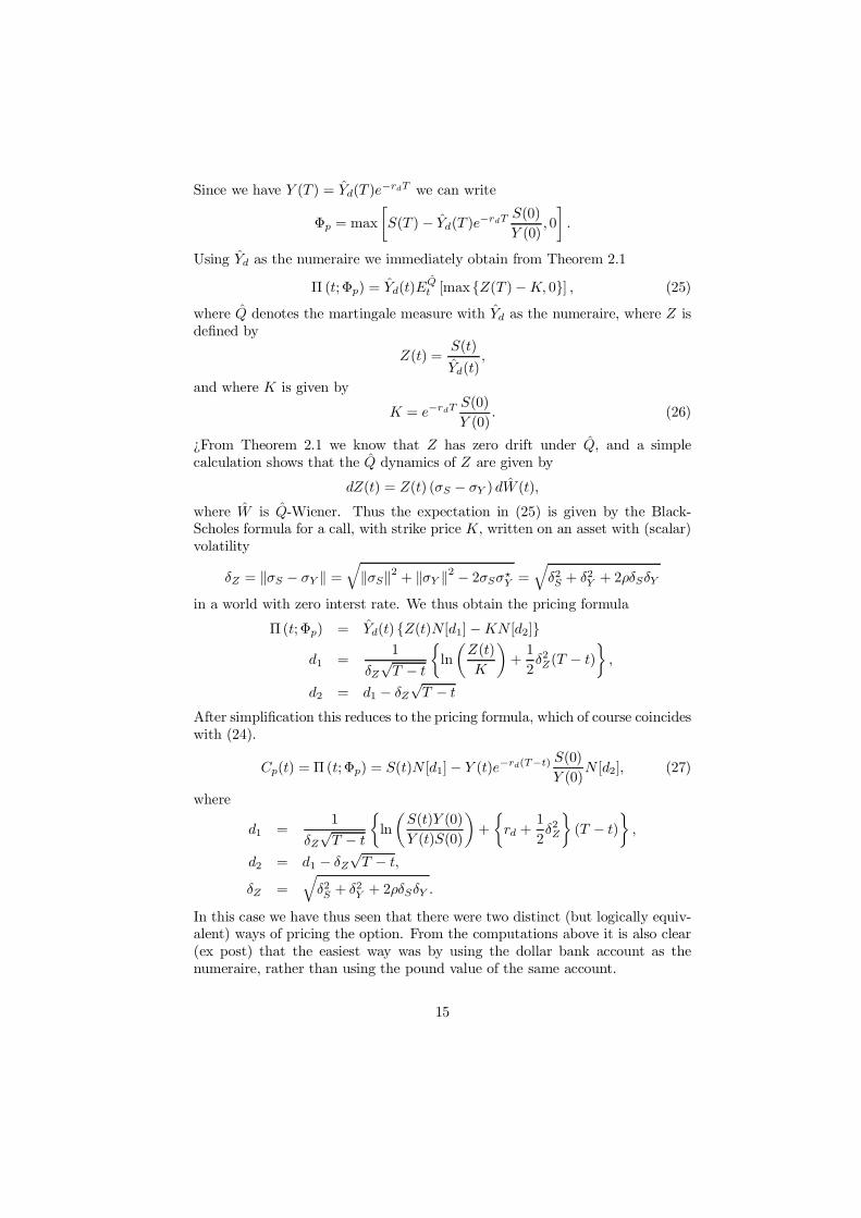
Since we have Y (T ) = Yd(T )e¡rdT we can write

©p = max

·S(T ) ¡ Yd(T )e¡rdT S(0)

Y (0); 0

¸:

Using Yd as the numeraire we immediately obtain from Theorem 2.1

¦ (t; ©p) = Yd(t)EQt [maxfZ(T )¡ K; 0g] ; (25)

where Q denotes the martingale measure with Yd as the numeraire, where Z isde¯ned by

Z(t) =S(t)

Yd(t);

and where K is given by

K = e¡rdT S(0)

Y (0): (26)

>From Theorem 2.1 we know that Z has zero drift under Q, and a simplecalculation shows that the Q dynamics of Z are given by

dZ(t) = Z(t) (¾S ¡ ¾Y ) dW (t);

where W is Q-Wiener. Thus the expectation in (25) is given by the Black-Scholes formula for a call, with strike price K, written on an asset with (scalar)volatility

±Z = k¾S ¡ ¾Y k =qk¾Sk2 + k¾Y k2 ¡ 2¾S¾?

Y =q

±2S + ±2

Y + 2½±S±Y

in a world with zero interst rate. We thus obtain the pricing formula

¦ (t; ©p) = Yd(t) fZ(t)N[d1] ¡ KN [d2]g

d1 =1

±Z

pT ¡ t

½ln

µZ(t)

K

¶+

1

2±2Z(T ¡ t)

¾;

d2 = d1 ¡ ±Z

pT ¡ t

After simpli¯cation this reduces to the pricing formula, which of course coincideswith (24).

Cp(t) = ¦(t; ©p) = S(t)N [d1] ¡ Y (t)e¡rd(T¡t) S(0)

Y (0)N [d2]; (27)

where

d1 =1

±Z

pT ¡ t

½ln

µS(t)Y (0)

Y (t)S(0)

¶+

½rd +

1

2±2Z

¾(T ¡ t)

¾;

d2 = d1 ¡ ±Z

pT ¡ t;

±Z =q

±2S + ±2

Y + 2½±S±Y :

In this case we have thus seen that there were two distinct (but logically equiv-alent) ways of pricing the option. From the computations above it is also clear(ex post) that the easiest way was by using the dollar bank account as thenumeraire, rather than using the pound value of the same account.

15

5 P r icing conver tible bonds

Standard pricing models of convertible bonds concentrate on pricing the bondand its conversion option at date t = 0 (see, for example, Brennan-Schwartz1977, Bardhan et.al. 1993). A somewhat less-standard problem is the pricing ofthe bond at some date 0 < t < T , where T is the maturity date of the bond. Weconsider this problem in this section; again we see that the numeraire approachgives a relatively simple solution to this problem; the "trick" is to use the stockprice as the numeraire. This gives a relatively simple pricing formula for thebond (equation (31) below), which we now derive.


A convertible bond involves two underlying objects: a discount bond and astock. The more precise assumptions are as follows.

² The bond is a zero coupon bond with face value 1.

² The bond matures at a ¯xed date T1.

² The underlying stock pays no dividends

² At a ¯xed date T0, with T0 < T1, the bond can be converted to one shareof the stock.

The problem is of course that of pricing, at time t < T0, the convertible bond.


We introduce the following notation

S(t) = the price, at time t, of the stock

p(t; T ) = the price, at time t, of a zero-coupon bond of the same risk class.

We now view the convertible bond as a contingent claim Y with exercise dateT0. Given the setup above, the claim Y is thus given by the expression

Y = max [S(T0); p(T0; T1)] :

In order to price this claim we have two obvious possibilities: we can use eitherthe stock or the zero-coupon bond maturing at T1 as the numeraire. Assumingthat the T1 bond actually is traded we immediately obtain the price as

¦ (t;Y ) = p(t; T1)E1t [max fZ(T0); 1g] ;

16

where E1 denotes expectation under the \forward neutral" martingale measureQ1 with the T1 bond as numeraire. The process Z is de¯ned by

Z(t) =S(t)

p(t; T1):

We can now simplify and write

max fZ(T0); 1g = max fZ(T0)¡ 1; 0g + 1;

giving us¦ (t; Y ) = p(t; T1)E

1t [max fZ(T0) ¡ 1; 0g] + p(t; T1) (28)

In more verbal terms this just says that the price of the convertible bond equalsthe price of a conversion option plus the price of the underlying zero couponbond. Since we assumed that the T1 bond is traded, we do not have to computethe price p(t; T1) in the formula above, but instead we simply observe the priceon the market. It thus only remains to compute the expectation above, and thisis obviously the price, at time t, of a European call with strike price 1 on theprice process Z in a world where the short rate equals zero. Thus the numeraireapproach gives a big simpli¯cation of the computational problem.

In order to obtain more explicit results, we now make more speci¯c assumptionsabout the stock and bond price dynamics.

Assumption 5.1 De¯ne, as usual, the forward rates by f(t; T ) = ¡ @@T

ln p(t; T );We now make the following assumptions, all under the risk neutral martingalemeasure Q.

² The bond market can be described by an HJM model for the forward ratesof the form

df(t; T ) =

Ã¾f (t; T )

Z T

t

¾0f(t; u)du

!dt + ¾f (t; T )dW (t)

where the volatility structure ¾f(t; T ) is assumed to be deterministic. Wis a (possibly multidimensional) Q-Wiener process.

² The stock price follows a geometric Brownian motion, i.e.

dS(t) = r(t)S(t)dt + S(t)¾SdW(t);

where rt = f(t; t) is the short rate. The row vector ¾S is assumed to beconstant and deterministic.

In essence we have thus assumed a standard Black-Scholes model for the stockprice S, and a Gaussian forward rate model. The point of this is that it willlead to (see below) a lognormal distribution for Z, thus allowing us to use a

17

standard Black-Scholes formula. From the forward rate dynamics above if nowfollows (BjÄork (1999), prop. 15.5) that we have bond price dynamics given by

dp(t; T ) = r(t)p(t; T )dt ¡ p(t; T )§p(t; T )dW (t);

where the bond price volatility is given by

§p(t; T ) =

Z T

t

¾f(t; u)du:

We may now attack the expectation in (28), and to this end we compute theZ-dynamics under QT1 . It follows directly from the Ito formula that the Q-dynamics of Z are given

dZ(t) = Z(t)®Z(t)dt + Zt f¾S + §p(t; T1)g dW (t)

where for the moment we do not bother about the drift process ®Z . Furthermorewe know from the general theory (see Theorem 2.1) that the following hold

² The Z process is a Q1 martingale (i.e. zero drift term).

² The volatility does not change when we change measure from Q to Q1.

The Q1 dynamics of Z are thus given by

dZ(t) = Z(t)¾Z(t)dW 1(t) (29)

where¾Z(t) = ¾S + §p(t; T1); (30)

and where W 1 is Q1-Wiener.

Under the assumptions above the volatility ¾Z is deterministic, thus guarantee-ing that Z has a lognormal distribution. We can in fact write

dZ(t) = Z(t) k¾Z(t)k dV 1(t);

where V 1 is a scalar Q1 Wiener process. We may thus use a small variation ofthe Black-Scholes formula to obtain the ¯nal pricing result

Proposition 5.1 The price, at t, of the convertible bond is given by the formula

¦(t; Y ) = S(t)N[d1] ¡ p(t; T1)N [d2] + p(t; T1);

where

d1 =1p

¾2(t; T0)

½ln

µS(t)

p(t; T1)

¶+

1

2¾2(t; T0)

¾;

d2 = d1 ¡p

¾2(t; T0);

¾2(t; T0) =

Z T0

t

k¾Z(u)k2 du;

¾Z(t) = ¾S +

Z T1

t

¾f(t; s)ds

18

6 P r icing savings plans with choice of linkage

These plans are common. Typically they give savers an ex-post choice of interestrates to be paid on their account. With the inception of capital requirements,many ¯nancial institutions have to recognize these options and price them.


We use the example of a common bank account from the Israeli context; thisaccount gives savers the ex-post choice of indexing their savings to an Israeli-shekel interest rate or a US dollar rate.

² The saver deposits NIS 100 (\NIS"= Israeli shekels) today in a shekel/dollarsavings account with a maturity of 1 year.

² In one year, the account pays the maximum of:

{ The sum of NIS 100 + real shekel interest, the whole amount indexedto the in°ation rate.

{ Today's dollar equivalent of NIS 100 + dollar interest, the wholeamount indexed to the dollar exchange rate.

The savings plan is thus an option to exchange the Israeli interest rate for theUS interest rate, while at the same time taking on the exchange rate risk. Sincethe choice is made ex-post, it is clear that both the shekel and the dollar interestrates o®ered on such an account must be below their respective market rates.


In this section we derive the value of the exchange option described above; theresult is given in equation (35) below.

We consider two economies, one domestic and one foreign, and we introduce thefollowing notation.

rd = domestic short rate

rf = foreign short rate

I(t) = domestic in°ation process

X(t) = the exchange rate in terms of domestic currency/foreign currency.

Y (t) = X(t)¡1 = the exchange rate in terms of foreign currency/ domestic currency.

T = the maturity of the savings plan.

The value of the option is linear in the initial shekel amount invested in thesavings plan; without loss in generality, we assume that this amount is 1 shekel.

19

In the domestic currency the contingent T -claim ©d to be priced, is thus givenby

©d = max£erdT I(T ); X(0)¡1erfT X(T )

¤

In the foreign currency the claim ©f is given by

©f = max£erdT I(T )Y (T ); Y (0)erf T

¤

It turns out that it is easier to work with ©f than with ©d, and we have

©f = max£erdT I(T )Y (T )¡ Y (0)erfT ; 0

¤+ Y (0)erfT :

The price (in the foreign currency) at t = 0 of this claim is now given by

¦ (0;©f ) = e¡rf T EQf£max

©erdT I(T )Y (T )¡ erf T Y (0); 0

ª¡ erfT Y (0)

¤

= EQf

hmax

ne(rd¡rf )T I(T )Y (T ) ¡ Y (0); 0

oi+ Y (0); (31)

where Qf denotes the risk neutral martingale measure for the foreign market.

At this point we have to make some probabilistic assumptions, and in fact weassume that we have a Garman-Kohlhagen model for Y . Standard theory thengives us the Qf dynamics of Y as

dY (t) = Y (t)(rf ¡ rd)dt + Y (t)¾Y dW (t): (32)

For simplicity we assume that also the in°ation follows a geometric Brownianmotion, with Qf -dynamics given by

dI(t) = I(t)®Idt + I(t)¾IdW (t): (33)

Note that W is assumed to be two-dimensional, thus allowing for correlationbetween Y and I. Also note that economic theory does not say anything aboutthe mean in°ation rate ®I under Qf .

When computing the expectation in (31) we cannot use a standard change ofnumeraire technique, the reason being that none of the processes Y , I or Y ¢I areprice processes of traded assets without dividends. Instead we have to attackthe expectation directly.

To that end we de¯ne the process Z as Z(t) = Y (t)¢I(t) and obtain the followingQf -dynamics.

dZ(t) = Z(t) (rf ¡ rd + ®I + ¾Y ¾0I) dt + Z(t) (¾Y + ¾I) dW (t):

>From this it is easy to see that if we de¯ne S(t) by

S(t) = e¡(rf¡rd + ®I + ¾Y ¾ 0I)tZ(t);

then we will have the Qf -dynamics

dS(t) = S(t) (¾Y + ¾I) dW (t);

20

the point being that we can interperet S(t) as a stock price in a Black-Scholesworld with zero short rate and Qf as the risk neutral measure. With thisnotation we obtain easily

¦ (0; ©f) = ecT EQf£max

£S(T )¡ e¡cT Y (0); 0

¤¤+ Y (0);

wherec = ®I + ¾Y ¾0

I :

The expectation above can now be expressed by the Black-Scholes formula fora call option with strike price e¡cT Y (0), zero short rate and a volatility givenby

¾ =q

k¾Y k2 + k¾Ik2 + 2¾Y ¾0I

The price, at t = 0 of the claim, expressed in the foreign currency is thus givenby the formula

¦ (0; ©f) = ecT I(0)Y (0)N [d1] ¡ Y (0)N [d2] + Y (0); (34)

d1 =ln (I(0)) +

¡c + 1

2¾2

¢T

¾p

T;

d2 = d1 ¡ ¾p

T :

Finally, the price at t = 0 in domestic terms is given by

¦ (0; ©d) = X(0)¦ (0;©f ) = ecT I0N [d1] ¡ N[d2] + 1: (35)

Remark 6.1 For practical purposes it may be more convenient to model Y andI as

dY (t) = Y (t)(rf ¡ rd)dt + Y (t)¾Y dWY (t);

dI(t) = I(t)®Idt + I(t)¾IdWI (t);

where now ¾Y and ¾Y are constant scalars, whereas WY and W I are scalarWiener processes with local correlation given by dWY (t)dW I(t) = ½dt.

In this model (which of course is logically equivalent to the one above) we havethe pricing formulas (34)-(35), but now with the notation

c = ®I + ½¾Y ¾I ;

¾ =q

¾2Y + ¾2

I + 2½¾Y ¾I

7 E ndowment war r ants

Endowment options, which are primarily traded in Australia and New Zealand,are very long-term call options on equity. These options were recently discussed

21

in this journal by Hoang-Powell-Shi (1999, henceforth HPS). Endowment war-rants have two unusual features: Their dividend protection consists of adjust-ments to the strike price, and the strike price behaves like a money market fund(i.e., increases over time at the short-term interest rate). HPS assume thatthe dividend adjustment to the strike price is equivalent to the usual dividendadjustment to the stock price; this assumption is now known to be mistaken.4

Under this assumption they prove an arbitrage-free warrant price for the casewhere the short-rate is deterministic and provide an approximation of the optionprice for the stochastic interest rate.

In this section we discuss a "pseudo-endowment option." This pseudo-endowmentoption is like the Australian option except that its dividend protection is theusual adjustment to the stock price (i.e., the stock price is raised by the divi-dends). The "pseudo-endowment option" thus depends on two sources of un-certainty: the (dividend-adjusted) stock price and the short-term interest rate.With a numeraire approach we can eliminate one of these sources of risk. Choos-ing an interest-rate related instrument (i.e., a money-market account) as a nu-meraire results in a pricing formula for the "pseudo-endowment option" whichis similar to the standard Black-Scholes formula.5


A pseudo-endowment option is a very long term call option. Typically we havethe following setup:

² At issue, the initial strike price K(0) is set to approximatively 50% ofthe current stock price, so the option is initially deep in the money.

² The endowment options are European.

² The time to exercise is typically 10+ years.

² The options are interest rate and dividend protected. The protection isperformed by the following two adjustments:

{ The strike price is not ¯xed over time. Instead it is increased by theshort-term interest rate.

{ The stock price is increased by the size of the dividend each time adividend is paid.

² The payo® at the exercise date T is that of a standard call option, butwith the adjusted (as above) strike price K(T ).

4 S ee "Div id en d P r otection at a P r ice: Lesson s fr om E n d ow m en t W ar r an ts," C h r istin eB r ow n an d Kev in Dav is, m im eo, Mar ch 2001, for th com in g in th is jou r n al?

5 T h is for m u la w as d er iv ed b y H P S as a solu tion for th e d eter m in istic in ter est r ate.

22


We model the underlying stock price process S(t) in a standard Black-Scholessetting. In other words, under the objective probability measure P , the priceprocess S(t) follows Geometrical Brownian Motion (between dividends) as:

dS(t) = ®S(t)dt + S(t)¾W p(t);

where ® and ¾ are deterministic constants and W p is a P Wiener process. Weallow the short rate r to be an arbitrary random process, thus giving us thefollowing P -dynamics of the money-market account:

dB(t) = r(t)B(t)dt; (36)

B(0) = 1: (37)

In order to analyze this option we have to formalize the protection features ofthe option. This is done in the following way.

² We assume that the strike price process K(t) is changed at the continu-ously compounded instantaneous interest rate. The formal model is thusas follows

dK(t) = r(t)K(t)dt: (38)

² For simplicity we assume (see Remark 7.1 below) that the dividend pro-tection is perfect. More precisely we assume that the dividend protectionis done by reinvesting the dividends into the stock itself. Under this as-sumption we can view the stock price as the theoretical price of a mutualfund which includes all dividends invested in the stock. Formally this im-plies that we can treat the stock price process S(t) de¯ned above as theprice process of a stock without dividends.

The value of the option at the exercise date T is given by the contingent claimY , de¯ned by

Y = max [S(T )¡K(T ); 0]

Clearly there are two sources of risk in endowment options: The stock price riskand the risk of the short-term interest rate. In order to analyze this option, weobserve that from (36)-(38) it follows that

K(T ) = K(0)B(T ):

Thus we can express the claim Y as

Y = max [S(T ) ¡K(0)B(T ); 0]

and from this expression we see that the natural numeraire process is nowobviously the money account B(t). The martingale measure for this numeraire

23

is the standard risk neutral martingale measure Q under which we have thestock price dynamics

dS(t) = r(t)S(t)dt + S(t)¾dW (t); (39)

where W is a Q-Wiener process.

A direct application of Theorem 2.1 gives us the pricing formula

¦ (0; Y ) = B(0)EQ

·1

B(T )max [S(T )¡K(0)B(T ); 0]

¸:

After a simple algebraic manipulation, and using the fact that B(0) = 1, wethus obtain

¦ (0;Y ) = EQ [max [Z(T )¡ K(0); 0]] (40)

where Z(t) = S(t)=B(t) is the normalized stock price process. It follows imme-diately from (36), (39), and the Ito formula that under Q we have Z-dynamicsgiven by

dZ(t) = Z(t)¾dW (t): (41)

and from (40)-(41) we now see that our original pricing problem has been re-duced to that of computing the price of a standard European call, with strikeprice K(0), on an underlying stock with volatility ¾ in a world where the shortrate is zero. Thus the Black-Scholes formula gives the endowment warrant priceat t = 0 directly as

CEW = ¦(0;Y ) = S0N(d1)¡K0N(d2) (42)

where

d1 =ln (S(0)=K(0)) + 1

2¾2T

¾p

T;

d2 = d1 ¡ ¾p

T :

Using the numeraire approach price of the endowment option in (42) is givenby a standard Black-Scholes formula for the case where r = 0. The result doesnot in any way depend upon assumptions made about the stochastic short rateprocess r(t).

The pricing formula (42) was in fact earlier derived in HPS, but only for thecase of a deterministic short rate. The case of a stochastic short rate is nottreated in detail in HPS. Instead the authors of HPS attempt to include thee®ect of a stochastic interest rate by introducing the following scheme:

² They assume that the short rate r is deterministic and constant.

² The strike price process is assumed to have dynamics of the form

dK(t) = rK(t)dt + °dV (t)

where V is a new Wiener process (possibly correlated with W ).

24

² They then go on to value the claim Y = max [S(T ) ¡K(T ); 0] by usingthe Margrabe (1978) result about exchange options.

The claim made in HPS is that this setup is an approximation to the case ofa stochastic interest rate. Whether it is a good approximation or not is neverclari¯ed in HPS, and from our analysis above we see that the entire schemeis in fact unnecessary, since the pricing formula (42) is invariant under theintroduction of a stochastic short rate.

Remark 7.1 We note that the result above relies upon our simplifying as-sumption about perfect dividend protection. A more realistic modeling of thedividend protection would lead to severe computational problems. To see thisassume that the stock pays a constant dividend yield rate ±. This would changeour model in two ways: The Q-dynamics of the stock price would be di®erent,and the dynamics of the strike process K(t) would have to be changed.

As for the Q-dynamics of the stock price, standard theory immediately gives us

dS(t) = (r(t)¡ ±)S(t)dt + S(t)¾dW (t):

Furthermore, from the institutional description above we see that in real life(as opposed to in our simpli¯ed model), the dividend protection is done bydecreasing the strike price process with the dividend amount at every dividendpayment. In terms of our model this means that over an in¯nitesimal interval[t; t + dt], the strike price should decrease with the amount ±S(t)dt. Thus theK-dynamics are given by

dK(t) = [r(t)K(t) ¡ ±S(t)] dt:

This equation can be solved as

K(T ) = eR

T

0r(t)dt

K(0)¡ ±

Z T

0

eR

T

tr(u)du

S(t)dt

The moral is that in the expression of the contingent claim

Y = max [S(T )¡K(T ); 0]

we now have the unpleasant integral expression

Z T

0

eR T

tr(u)du

S(t)dt:

Even in the simple case of a deterministic short rate this integral is quite prob-lematic. It is then basically a sum of lognormally distributed random variables,and thus we have the same hard computational problems as in the case of anAsian option.

25

8 Conclusion

Numeraire methods have been in the derivative pricing literature since papersby Geman (1989) and Jamshidian (1989). These methods a®ord a considerablesimpli¯cation in the pricing of many complex options; however, they appearnot to be well-known. In this paper we have considered ¯ve problems whosecomputation is vastly aided by the use of numeraire methods. The ¯rst of theseis the pricing of endowment options (discussed in the Journal of Derivatives ina recent paper by Hoang, Powell, and Shi (1999). We also discuss the pricing ofoptions where the strike price is denominated in a currency di®erent from thatof the underlying stock, the pricing of savings plans where the choice of interestpaid is ex-post chosen by the saver, the pricing of convertible bonds and thepricing of employee stock ownership plans.

Numeraire methods are not a panacea for complex option pricing. However,when there are several risk factors which impact an option's price, choosing oneof the factors as a numeraire reduces the dimensionality of the computationalproblem by one. A clever choice of the numeraire can, in addition, lead to asigni¯cant computational simpli¯cation in the option's pricing.

Refer ences

[1] Bardhan I., A. Bergier, E. Derman, C. Dosemblet, I Kani, P. Karasinski(1993). Valuing convertible bonds as derivatives. Goldman Sachs Quanti-tative Strategies Research Notes.

[2] BjÄork T. (1999). Arbitrage Theory in Continuous Time, Oxford UniversityPress.

[3] Brennan M.J., E.S. Schwartz (1977). Convertible bonds: Valuation andoptimal strategies for call and conversion. The Journal of Finance, 32,1699-1715.

[4] Brenner, M., D. Galai (1978). The Determinants of the Return on IndexBonds. Journal of Banking and Finance, 2, 47-64.

[5] Brown, C., K. Davis (2001). Dividend Protection at a Price: Lessons fromEndowment Warrants, working paper.

[6] Core J., W. Guay (2000). Stock Option Plans for Non-Executive Employees,Working paper, Wharton School.

[7] Fischer, S. (1978). Call option pricing when the exercise price is uncertain,and the valuation of index bonds. Journal of Finance, 33, 169-176.

[8] Geman, H. (1989). The Importance of the Forward Neutral Probability ina Stochastic Approach of Interest Rates. Working paper, ESSEC.

26

[9] Geman, H., N. El Karoui and J. C. Rochet (1995). "Change of Numeraire,Changes of Probability Measures and Pricing of Options." Journal of Ap-plied Probability, 32, 443-458.

[10] Harrison, J. & Kreps, J. (1981). Martingales and Arbitrage in MultiperiodSecurities Markets. Journal of Economic Theory 11, 418{443.

[11] Harrison, J. & Pliska, S. (1981). Martingales and Stochastic Integrals inthe Theory of Continuous Trading. Stochastic Processes & Applications11, 215{260.

[12] Haug E. G. (1997), The complete guide to option pricing formulas, McGrawHill.

[13] Heath C., S. Huddart, and M. Lang (1999). Psychological factors and stockoption exercise, Quarterly Journal of Economics, 114, 601-628.

[14] Hoang, Philip, John G. Powell, and Jing Shi (1999). Endowment WarrantValuation, Journal of Derivatives, 91-103.

[15] Huddart S. (1994). Employee stock options, Journal Of Accounting AndEconomics 18, 2, 207-231.

[16] Jamshidian, F. (1989). An Exact Bond Option Formula. Journal of Finance44, 205{209.

[17] Margrabe W. (1978). The value of an option to exchange one asset foranother, Journal of Finance, 33, 1, 177-186.

[18] Reiner E. (1992). Quanto mechanics, Risk Magazine, 5, 59-63.

27

o n the use of numeraires in o ption...

Documents