oar lib: an open source arc routing library
TRANSCRIPT

Mathematical Programming Computation (2019) 11:587–629https://doi.org/10.1007/s12532-019-00155-5
FULL LENGTH PAPER
OAR Lib: an open source arc routing library
Oliver Lum1 · Bruce Golden2 · Edward Wasil3
Received: 24 July 2017 / Accepted: 5 February 2019 / Published online: 27 March 2019© Springer-Verlag GmbH Germany, part of Springer Nature and Mathematical Optimization Society 2019
AbstractWe present an open source, arc routing Java library that has a flexible grapharchitecture with solvers for several uncapacitated arc routing problems and the abil-ity to dynamically generate and visualize real-world street networks. The libraryis hosted at https://github.com/Olibear/ArcRoutingLibrary (https://doi.org/10.5281/zenodo.2561406). We describe the algorithms in the library, report computationalperformance, and discuss implementation issues.
Mathematics Subject Classification 90B06 · 90B10 · 90C27 · 90C59
1 Introduction
In vehicle routing, problem complexity (e.g., costs, constraints such as time windows,etc.) is associated with the nodes and the edges of the underlying street network.Problem variants where vehicles service customers at the nodes are referred to asnode routing problems. These include the traveling salesman problem and the vehiclerouting problem. Variants where customers lie on the edges are referred to as arcrouting problems. In both cases, the goal is to minimize an objective function thatreflects the total cost of the routes.
Nearly all routing problems have been shown to be NP-Hard, so it is unlikely thatthey can be solved to optimality in a computationally tractable manner [11]. Heuris-
B Oliver [email protected]
Bruce [email protected]
Edward [email protected]
1 Department of Applied Mathematics and Scientific Computation, University of Maryland,College Park, MD, USA
2 Robert H. Smith School of Business, University of Maryland, College Park, MD, USA
3 Kogod School of Business, American University, Washington, DC, USA
123

588 O. Lum et al.
tics avoid this intractability by finding very good solutions that are nearly optimal.Heuristics are evaluated based on efficiency and accuracy.
Different implementations of the same algorithm can lead to different results, butthis variability is difficult to control. For example, differences in data structures andhow memory is managed can drastically affect the runtime required to solve a partic-ular instance. The effect of these differences is more apparent when these heuristicsare used as subroutines. For example, suppose there are two competing metaheuristicsA and B. Both solve a shortest paths problem during their respective initializationprocedures. Since the researcher responsible for A uses a more efficient shortest pathsalgorithm, significantly faster runtimes are reported. However, if this difference wereeliminated, A would be slower than B. One would reasonably, but erroneously, con-clude that metaheuristic A is superior. Therefore, it is important to standardize solversso that fair comparisons can be made and the merits of an algorithm can be attributedsolely to its design.
We develop an open source code library that provides a set of standard solvers forarc routing problems. The library contains solvers for the following problems: theChinese Postman Problem on a directed graph (DCPP), the CPP on an undirectedgraph with symmetric traversal costs (UCPP), the CPP on a mixed graph (MCPP),the CPP on an undirected graph with directionally asymmetric costs (WPP for WindyPostman Problem), and the Rural Postman Problem (RPP) on directed (DRPP) andwindy graphs (WRPP) where not all arcs are required to be traversed in the solution.For each problem, if it is not possible to efficiently solve it to optimality, we implementa well-known heuristic in our library. If the problem is solvable in polynomial time,we implement the exact algorithm in our library. For the details of each specificalgorithm, consult references for the DCPP, UCPP, MCPP, WPP, DRPP, and WRPP[4,5,10,14,17,30–32]. In Table 1, we summarize the problems that are addressed inthe library. In Table 2, we summarize the performance of the heuristics contained inthe library. We point out that the paper by Groër et al. [16] is a companion paper thatpresents a library of local search heuristics for node routing problems.
Table 1 Problems addressed by the library
Problem Required links Exact solver Heuristics References
Directed Chinese postman problem All 1 0 [10]
Undirected Chinese postman problem All 1 0 [10]
Mixed Chinese postman problem All 0 2 [14,32]
Windy postman problem All 0 2 [4,31]
Directed rural postman problem Subset 0 1 [5]
Windy rural postman problem Subset 0 1 [4]
A summary of the problems addressed in the library. The required links column shows whether all links inthe graph require traversal, or only a subset require traversal. The exact solver column shows the problemsthat can be solved exactly in the library. The heuristics column shows the number of heuristics in the libraryfor each problem. The references column provides the original source of the algorithms
123

OAR Lib: an open source arc routing library 589
Table 2 Performance measures for heuristics in the library
Solver Average deviation (%) Max deviation (%) Benchmarkinstances
References
Frederickson’sheuristic for theMCPP
15.9 78.0 Manhattan,complete, andspecial case
[32]
Yaoyuenyong etal.’s heuristic forthe MCPP
1.0 14.4 Manhattan,complete, andspecial case
[32]
Christofides’sheuristic for theDRPP
24.23 64.11 Campos andSavall
[5]
Benavent et al.’sheuristic for theWRPP
4.17 Not provided Albaida–Madrigueras
[4]
A computational summary of the heuristics in the library. Deviations are percentages from lower boundspresented in the cited reference. These are the results from running each solver on the test data sets in thebenchmark instances column. Note that the references in this table are to the papers which provide thecomputational results listed here. For the references which introduce the heuristics, consult Table 1
1.1 Definitions
A graph G = (V , L) where V is a set of vertices (also referred to here as nodes) andL is a set of links. Vertices are defined by vi and links are represented as ordered pairsli j = (i, j) where both vi and v j are members of the vertex set. A link l = (i, j)also has a traversal cost ci j . A link is an edge if it is undirected (it can be traversedfrom vi to v j and from v j to vi ). Edges are denoted by ei j . A link is an arc if it isdirected (it can only be traversed from vi to v j ). Arcs are denoted by ai j . In the caseof arcs, the first element of the ordered pair is referred to as the tail, while the secondis referred to as the head. In an undirected graph, all members of the link set are edgesand the graph is denoted by (V , E). In a directed graph, all members of the link setare arcs, and the graph is denoted by (V , A). A mixed graph has both types of linksand is denoted by (V , E, A). A windy graph is undirected with asymmetric traversalcosts (the cost of going from vertex vi to vertex v j may not be the same as the cost ofgoing from vertex v j to vertex vi ).
Awindy graph canmodel an undirected graph, a directed graph, and amixed graph.For an undirected graph, set ci j = c ji ∀i, j ; for a directed graph, set ci j to be the costof ai j , and c ji = N ∀a = (i, j) ∈ A where N is a very large value, much greater than∑
ai j∈A ci j ; for a mixed graph, it follows directly from the previous two graph types.Thus, any solution method that can be applied to a problem on a windy graph can alsobe applied to the same problem on the three types of graphs.
In an undirected graph, the degree of a vertex is simply the number of edges incidentto the vertex. In a directed graph, the in-degree of a vertex v is the number of arcs a ∈ Afor which v is the head, and the out-degree of a vertex v is the number of arcs for whichv is the tail. For a mixed graph, our definition of in-degree and out-degree remain thesame. The two properties only take into account arcs in the graph, while our definitionof degree only includes edges as though the arcs were deleted from the graph.
123

590 O. Lum et al.
A graph is strongly connected if it is possible to reach any vertex from any othervertex. For any pair of vertices vi and v j , it is possible to construct an ordered list ofvertices vi , . . . , v j , where vertices that are adjacent in the list are connected by a link.An ordered list of this form is called a path. A path with minimal traversal cost in thegraph is known as a shortest path. We denote the cost of a shortest path between vertexvi and vertex v j as spi j .
A circuit is defined as a path that begins and ends at the same vertex. A graph isEuler if and only if there exists an Euler circuit, i.e., a circuit that traverses every linkin the graph exactly once. The following is a list of well-known conditions for a graphto be Euler.
• Undirected: An undirected graph is Euler if and only if every node has even degree(a property known as evenness).
• Directed: A directed graph is Euler if and only if the in-degree equals the out-degree for every node (a property known as symmetry).
• Mixed: A mixed graph is Euler if and only if every node has even degree and thegraph is balanced. For any subset S of V , |number of arcs from S to V \S-numberof arcs from V \S to S| ≤ number of edges from S to V \S. A sufficient conditionis that every node has even degree, and the in-degree equals the out-degree.
A graphG2 = (V2, L2) is an augmentation of the graphG1 = (V1, L1) if V1 ⊆ V2,L1 ⊆ L2, and ∀l2i j ∈ L2, ∃ l1i j ∈ L1 and cost(l2i j ) = cost(l1i j ). Every link in theoriginal graph appears in the augmentation. The augmentation only includes copiesof links in the original graph.
The problems we consider fall under the following two categories.
• Chinese Postman Problem: Given a graph G (either directed, undirected, mixed,or windy) and a cost function ci j (associated with traversing the link (i, j)), find acircuit that traverses each link (edge or arc) at least once and minimizes the totaltraversal cost.
• Rural Postman Problem: Given a graph G (either directed or windy), a set ofrequired links LR ⊆ L , a depot location (one of the vertices), and cost functionci j (associated with traversing the link (i, j)), find a circuit beginning and endingat the depot that traverses each required arc at least once and minimizes the totaltraversal cost.
In both the CPP and the RPP, the problem is solved in two steps. First, find an Euleraugmentation of the original graph. Second, find the Euler circuit in the augmentedgraph. The second step can be performed easily and efficiently in linear time usingHierholzer’s algorithm [19].
We use the following common notation.
• δ(v) = in-degree minus the out-degree,• D+ and D− are the set of vertices with δ(v) > 0 and δ(v) < 0,• Z
0+ is the set of non-negative integers (N).
123

OAR Lib: an open source arc routing library 591
Fig. 1 Agraph fromOSM thatwas generated by querying the street network of Perth, Australia and exportedthrough the Gephi integration
2 Features of the library
We now describe some of the features in our library.In order to depict networks and the corresponding vehicle routes, we use Gephi
[3]. Gephi is an open source visualization utility with an application programminginterface (API) that enables quick integration. Gephi allows several layout routinesthat attempt to minimize visual clutter while preserving distance relationships.
The library contains the ability to manually specify vertex coordinates. We usethese subroutines to export any graph created within the library to a portable documentformat (pdf) file.
To allow the quick, dynamic generation of new test instances, we have leveragedthe queryable Open Street Maps (OSM) [18] database to allow a user with an Internetconnection to specify a geographic bounding box and retrieve the associated streetnetwork. The largest contiguous subgraph is returned so that connectivity is ensured.Figure 1 gives a street network returned by OSM sampling a portion of the streetnetwork in Perth, Australia.
We have decoupled seven graph algorithms that are used in multiple solvers toallow for them to be used in contexts not originally coded by the authors, includinginside more sophisticated solvers. The worst-case computational complexity (using“big oh” notation) is provided after the name of each algorithm in the list below.
• Floyd–Warshall all-pairs shortest paths algorithm: O(|V |3) [13]• Dijkstra’s single-source shortest paths algorithm with priority queues: O(|E | +
|V | log |V |) [8]
123

592 O. Lum et al.
• Successive shortest paths min cost flow algorithm: O(|V |∗|E |∗B log |V |), whereB is the maximum supply [26]
• Blossom V min cost matching algorithm: O(|V |3 ∗ |E |) [21]• Hierholzer’s algorithm: O(|E |) [19]• Minimum spanning tree algorithm: O(|E | log |V |) [28]• Strongly connected components algorithm: O(|V | + |E |) [22]
3 Architecture
We discuss the structure of the library and outline how the core architecture can beextended to implement various solvers.
The library’s core package contains the abstractions upon which the rest of thelibrary is based. The graph, link, and vertex abstractions maintain a unique (per type)global identifier (ID). This ID may be used to compare elements that may otherwiseappear similar (e.g., when manipulating multiple graphs, both depots may be referredto as v1 but the global ID property will distinguish between the two). In addition, linksand vertices have a local ID. The local ID is based on the graph that the node or link isassigned to. Therefore, the first vertex assigned to each graph will have a local ID ofone. Finally, links and vertices may keep track of a match ID. The match IDmay be setto allow the correspondence between elements in a graph. For example, the solutionof a flow problem on an auxiliary graph can be used to construct an augmentation ofthe original graph. In this case, the match ID of edges in the original graph can be setto the local IDs of edges in the auxiliary graph to allow a user to keep track of thecorrespondence.
Graph objects maintain additional state information. The shortest path matrix isavailable on demand, and storage is implemented according to a lazy design pattern(the memory is not allocated until it is first needed, and only recomputed if the stateof the graph changes). The (local) ID of the depot and the element sets (V and E) aremaintained by the graph. Functions for standardized creation of vertices and links, aswell as getters (methods which allow other objects to retrieve a specific vertex or edge)are provided. Finally, a method for providing deep copy (a distinct copy as opposedto a reference to the existing object) is specified by all graphs.
The problem and solver abstractions are included in the core package. Probleminstances contain the underlying network, objective function, and any problem featuressuch as time windows and additional service costs. We restrict the ability of a solver toonly apply to those networks with certain structure via the checkGraphRequirementsmethod. This feature enables a solver to specify the conditions for a feasible solution(e.g., strong connectedness for solving the DCPP).
Improvement procedures are also implemented as an abstract class that allowsfor composition of improvement frameworks, as well as the composite local searchoperators. This creates an opportunity for both individual procedures (e.g., the arcrouting analog of a 2-opt) and frameworks (i.e., an ordered set of procedures withtermination criteria) to be modular when tuning a heuristic.
The mover object simplifies the accounting associated with writing improvementprocedures. It performs swaps for arc routing problems by manipulating routes as
123

OAR Lib: an open source arc routing library 593
ordered lists of required links (with shortest paths assumed in between), and inter-changing positions of the links in the lists. This compact representation of a route wasfirst proposed by Benavent et al. [4]. It allows for many improvement procedures fromnode routing to be used in an arc routing setting.
Wherever possible, we use fast and memory efficient data structures to organizeelements of the graph. For example, we use Trove [15] which provides memory-optimized variants of several native Java data structures to store vertices and edges.Elements are usually referenced via their local ID.We use these data structures to storegraphs using a structure similar to an adjacency list. Instead of storing pairs of adjacentnodes, we store a set of link objects. By adding this layer of abstraction, it is possibleto extend the architecture to support multigraphs and hypergraphs easily. Alternativerepresentations of the graph structure, such as sparse matrix representations, can haveincreased storage requirements, and can be difficult to adapt to graphs with multipleedges between vi and v j . Support for multigraphs is needed for the augment-routeapproach for solving an arc routing problem.
4 Problem setting and algorithms
In this section,we describe the problems and respective solvers that are implemented inthe library. In general, the algorithms proceed by augmenting the underlying networkto satisfy the requirements for the existence of an Euler circuit (i.e., the augmentedgraph is Euler) in a way that minimizes the aggregate cost of the added elements. Anoverview of the solution strategies is given in Table 3.
4.1 Directed Chinese postman problem
The DCPP is given by:
minimize∑
i or j∈{D+∪D−}ci j xi j (1)
subject to:∑
i∈D+xi j = −δ( j), ∀ j ∈ D− (2)
∑
j∈D−xi j = δ(i), ∀i ∈ D+ (3)
xi j ∈ Z0+ (4)
The variable xi j is the number of times a shortest path is added from node i to nodej in the augmented graph. ci j is the cost of the shortest path from node i to node j .The objective function (1) is the total additional cost incurred by the augmentation.Constraints (2) and (3) ensure that, after we have added these shortest paths, the graphis symmetric.
123

594 O. Lum et al.
Table 3 Solvers in the library
Solver Description
Edmonds andJohnson’s exactalgorithm for theDCPP [30]
Solve a min cost flow problem. Symmetry is achieved by adding arcs according tothe solution to the flow problem
Edmonds’s exactalgorithm for theUCPP [10]
Solve a min cost matching problem. Evenness is achieved by adding edgesaccording to the solution
Frederickson’sheuristic for theMCPP [14]
Use Edmonds’s algorithms for the UCPP and DCPP separately to achieve eachproperty. Repair the augmentation by eliminating special circuits in the graph
Yaoyuenyong etal.’s heuristic forthe MCPP [32]
Apply augmentation procedures from Frederickson’s heuristic. Applyimprovement procedures that search for opportunities to replace added linkswith shortest paths
Win’s heuristic forthe WPP [31]
Create an auxiliary undirected graph with cauxi j = .5 ∗ (ci j + c ji ). Solve theUCPP on the auxiliary graph. Augment the original graph according to theUCPP solution on the auxiliary graph. Solve a min cost flow problem on theaugmented original graph to produce the Euler circuit
Benavent et al.’sheuristic for theWPP [4]
As a preprocessor to Win’s heuristic, identify a set of edges for which |ci j − c ji | islarge relative to most other edges in the graph. Solve a min cost flow problem,assuming that these edges will be traversed in the cheaper direction. Then,proceed as in Win’s heuristic
Christofides’sheuristic for theDRPP [5]
Solve a min cost spanning arborescence on an auxiliary graph where each requiredconnected component from the original graph is collapsed into a single node.Mark arcs in the arborescence as required, and then solve the DCPP on theresulting graph. Repeat the process, rooting the arborescence in differentrequired connected components while keeping track of the best solution
Benavent et al.’sheuristic for theWRPP [4]
Solve a min cost spanning tree on an auxiliary graph where each requiredconnected component from the original graph is collapsed into a single node.Make each edge in the spanning tree solution required, and apply Benavent etal.’s WPP heuristic
A summary of the solvers in the library. Solution quality is given as average deviation from optimalitypresented in the cited references
4.1.1 Exact algorithm for the directed Chinese postman problem
We solve a min cost flow problem on the underlying directed graph (see Thimbleby[30]) where the supply of vertex i is given by δ(vi ). A vertex with a negative δ(vi )
indicates demand. For each unit of flow along an arc in the solution to the resultingflow problem, we add a copy of the arc to the graph. In this way, every vertex in theaugmented graph will have δ(v) = 0, ensuring that each time a vertex is visited, it ispossible to leave it along an arc that has not yet been traversed. It is also possible toshow that this a least-cost symmetric augmentation. Figures 2 and 3 show a small graphand the augmentation produced by the algorithm. The graph in Fig. 3 is symmetric and,therefore, has an Euler circuit. Pseudocode for this algorithm is given in Algorithm 1.
123

OAR Lib: an open source arc routing library 595
Fig. 2 An instance of the DCPP.The number inside a node is avertex id, while the numberadjacent to each arc denotes thecost of traversing thecorresponding arc. Since this is adirected graph, the arcs in thegraph can only be traversed inone direction, from the arrow tailto the arrow head
Fig. 3 The optimal solution tothe DCPP in Fig. 2. Node 5belongs to D+ and node 2belongs to D− in the initialphase of the algorithm. Arcsadded as part of the min costflow solution are shown asdotted arcs. The optimal Eulercircuit is1−2−5−3−4−5−3−1−2−3−1.The cost of the solution is thesum of the arc costs(2(2) + 2(1) + 1 + 2 + 2(1) +1 + 3 = 15)
Algorithm 1 DCPP Exact Solver1: procedure DCPP Edmonds and Johnson(G)2: for vertex v ∈ V do3: δ(v) ← in-degree − out-degree4: supply(v) ← δ(v)
5: end for6: Solve a min cost flow over G7: for i = 1 : |E | do8: for j = 1 : f low(ei ) do9: Add copy of ei to G10: end for11: end for12: Return Hierholzer(G)13: end procedure
Algorithm1:Outline of Edmonds and Johnson’s [30] exact algorithm for theDCPP.
123

596 O. Lum et al.
4.2 Undirected Chinese postman problem
The UCPP is given by:
minimize∑
(i, j)∈Eci j xi j (5)
subject to:∑
(i, j)∈Ev
(xi j + 1) ≡ 0 mod 2, ∀v ∈ V (6)
xi j ∈ Z0+ (7)
In this formulation, Ev is the set of edges incident to vertex v and xi j is the numberof additional copies of edge (i, j) in our augmented graph. We minimize the addedcost, while ensuring every vertex has even degree in the augmented graph (Constraint6 achieves this).
Fig. 4 An instance of the UCPP.The number inside a node is avertex id, while the numberadjacent to each edge denotesthe cost of traversing the edge
Fig. 5 The optimal solution tothe UCPP in Fig. 4. Nodes withdotted borders (1 and 2, in thiscase) are identified as odddegree nodes in the initial phaseof the algorithm. Edges thatwere added as part of thematching solution are shown asdotted lines
123
OAR Lib: an open source arc routing library 597
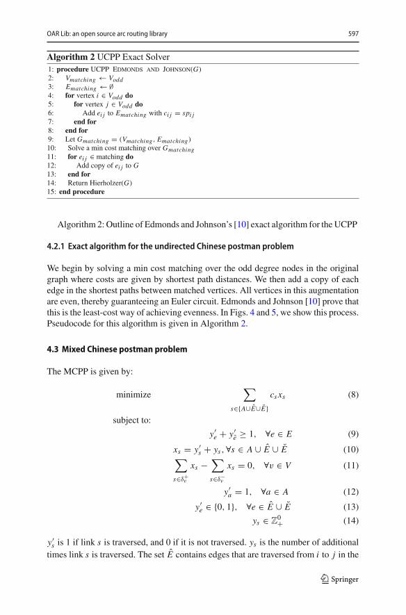
Algorithm 2 UCPP Exact Solver1: procedure UCPP Edmonds and Johnson(G)2: Vmatching ← Vodd3: Ematching ← ∅4: for vertex i ∈ Vodd do5: for vertex j ∈ Vodd do6: Add ei j to Ematching with ci j = spi j7: end for8: end for9: Let Gmatching = (Vmatching, Ematching)
10: Solve a min cost matching over Gmatching11: for ei j ∈ matching do12: Add copy of ei j to G13: end for14: Return Hierholzer(G)15: end procedure
Algorithm 2: Outline of Edmonds and Johnson’s [10] exact algorithm for theUCPP
4.2.1 Exact algorithm for the undirected Chinese postman problem
We begin by solving a min cost matching over the odd degree nodes in the originalgraph where costs are given by shortest path distances. We then add a copy of eachedge in the shortest paths between matched vertices. All vertices in this augmentationare even, thereby guaranteeing an Euler circuit. Edmonds and Johnson [10] prove thatthis is the least-cost way of achieving evenness. In Figs. 4 and 5, we show this process.Pseudocode for this algorithm is given in Algorithm 2.
4.3 Mixed Chinese postman problem
The MCPP is given by:
minimize∑
s∈{A∪E∪E}cs xs (8)
subject to:
y′e + y′
e ≥ 1, ∀e ∈ E (9)
xs = y′s + ys,∀s ∈ A ∪ E ∪ E (10)
∑
s∈δ+v
xs −∑
s∈δ−v
xs = 0, ∀v ∈ V (11)
y′a = 1, ∀a ∈ A (12)
y′e ∈ {0, 1}, ∀e ∈ E ∪ E (13)
ys ∈ Z0+ (14)
y′s is 1 if link s is traversed, and 0 if it is not traversed. ys is the number of additionaltimes link s is traversed. The set E contains edges that are traversed from i to j in the
123

598 O. Lum et al.
solution, while the set E contains edges that are traversed from j to i . Similarly, thesubscripts e and e correspond to traversing edge e forward (from i to j) and backward(from j to i), respectively. δ+
v and δ−v denote the set of edges and arcs which start at,
or end at, vertex v respectively. Therefore, xs is the total number of times link s istraversed. Constraint (9) ensures that each edge is traversed at least once. Constraint(10) defines xs . Constraint (11) ensures symmetry. Constraint (12) ensures that arcsare traversed at least once. Constraint (13) is the binary constraint for y′
s . Constraint(14) is the integrality constraint for the ys .
4.3.1 The even-symmetric-even heuristic
We augment the graph to produce an Euler graph in the hope of finding an Eulercircuit. Recall that in order for a mixed graph to be Euler, it must be balanced (i.e.,for each subset of nodes S, |{ei j ∈ E : i ∈ S and j ∈ V \S}| ≥ (|{ai j ∈ A : i ∈ S andj ∈ V \S}|− |{ai j ∈ A : i ∈ V \S and j ∈ S}|). Intuitively, this condition ensures thatthere are enough (undirected) edges to account for the difference between the numberof one-way streets in and out of a portion of the graph.
Checkingwhether amixed graph is balanced is computationally intractable becausethe number of subsets in S is exponential in the number of vertices in V . Therefore,the heuristic relies on the fact that it is sufficient but not necessary for a balanced graphto be even and symmetric (see Frederickson [14]).
The Even-Symmetric-Even heuristic has three phrases. In the first phase, it achievesevenness by carrying out a min cost matching among the odd vertices. In the secondphase, it achieves symmetry by using a min cost flow algorithm on the asymmetricnodes. In the third phase, it restores evenness by looking for circuits that may beeliminated while preserving the symmetry achieved in the second phase. This processis shown in Figs. 6 and 7. Pseudocode for this heuristic is given in Algorithm 3.
1. Phase I, Even. Solve the UCPP on the original graph by treating all arcs as edges.This produces an augmented graph GE .
2. Phase II, Symmetric. Solve a min cost flow problem on GE by treating each edge(u, v) as four arcs (the first two (u, v) and (v, u) with cost equal to the original
Fig. 6 An instance of the MCPP.The number inside the node is avertex id, while the numberadjacent to each link denotes thecost of traversing thecorresponding link. Arrowsdenote arcs that can only betraversed from tail to head, whilelines without arrows denoteedges
123

OAR Lib: an open source arc routing library 599
Fig. 7 A solution to the MCPPinstance in Fig. 6 procduced byFrederickson’s algorithm [14].The dotted arc (2, 5) is added inthe initial Even phase, while allother dotted arcs are added inthe Symmetric phase. Thedouble arrows (3, 4) and (3, 2)indicate that the edges in theoriginal graph were oriented inthe corresponding direction
edge cost and infinite flow capacity, and two (u, v) and (v, u) with zero cost, andflow capacity of 1). In the flow solution, if arc (u, v) is traversed only once, or arc(v, u) is traversed only once, then we orient the edge in that direction; otherwiseedge (u, v) remains as an edge in our output graph GS .
3. Phase III, Even: Using a greedy procedure, search for circuits that have pathsbetween any odd-degree nodes left in GS . If there are none, Phase III is skipped.These paths must alternate between using arcs or oriented edges added in Phase II,and using edges left undirected by Phase II. For example, if there were four odd-degree nodes remaining (v1, v2, v3, v4), an eligible circuit would be a path fromv1 to v2 of added arcs, a path from v2 to v3 of unoriented edges, a path from v3 tov4 of added arcs, and a path from v4 to v1 of unoriented edges. This ensures thatonly the parity of the odd-degree nodes is changed, while assigning a directionto all remaining undirected edges. After we find one of these alternating paths,we orient it (either direction will be equivalent) and duplicate arcs and orientededges along the path that follow the orientation, while deleting arcs that are in theopposite direction. For the segments of the circuit that have edges, we orient themin the direction we have chosen to orient the circuit.
Algorithm 3MCPP Heuristic Solver1: procedure MCPP Frederickson(G)2: GE ← EvenDegree(G)
3: GS ← Symmetric(GE )
4: G f inal ← EvenPari ty(GS)
5: Return Hierholzer(G f inal )6: end procedure
Algorithm 3: Outline of Frederickson’s heuristic [14] for the MCPP
123

600 O. Lum et al.
4.3.2 Shortest additional path heuristic
The initial step of theShortestAdditional PathHeuristic (SAPH, [32]) is identical to thesecond phase of the Even-Symmetric-Even heuristic where the graph is transformedinto a symmetric one.After this phase is completed, links in the graph are characterizedas belonging to one of six categories shown in Fig. 8. These categories are based onhowmany copies of a given link have been added in the augmentation in the first phase,and, in the case of an edge, which direction it has been assigned. The remaining phasesof the algorithm attempt to delete some of these added links by adding and subtractingpaths in the graph.
This second phase begins by exploiting two ideas. First, suppose that an edge orarc was added to the original graph, and oriented from node i to node j . If the shortestpath cost from node i to j is less than the cost of traversing this added link, then wereplace the link with the shortest path from i to j (see Fig. 9). We call this shortestpath replacement. Pseudocode for this procedure is given in Algorithm 4. Second, if anedge in the original graph was oriented from node i to j , we consider the possibility ofdeleting some added links by reversing the orientation of the edge. For each orientedcopy of an edge or arc (denoted by acopyi j ) added as part of the augmentation, consider
a virtual arc avj i in the opposite direction with cost equal to −ccopyi j . Then, compute
the shortest path from i to j which we call sp1i j with cost csp1. Delete each virtual
arc traversed in sp1i j . Again, compute the shortest path from i to j , (which may bedifferent now that some of the negative cost virtual arcs have been removed). We callthis shortest path sp2i j , with cost csp2. If csp1 + csp2 < 0, then it is advantageous totraverse the shortest path from i to j , service the edge in the opposite direction (fromj to i), and then traverse the second shortest path from i to j . For each actual edge insp1i j and sp
2i j , a copy is added and for each virtual edge, a copy is deleted. For example,
in Fig. 10, two paths from v1 to v2 are added. One of these paths costs − 7. Supposethat an arc of cost 9 from v4 to v3 was added in the first phase of the heuristic and thatc13 = c42 = 1. Then, the path v1 − v3 − v4 − v2 would have cost 1− 9+ 1 = −7. Wecall this procedure reversal. Pseudocode for this procedure is given in Algorithm 5.
With this notation and these procedures established, we now describe SAPH.
1. Given a mixed graph G, generate a graph G∗ = (N , M,U ) and a set of addedarcs M∗ by solving Phase II of Even-Symmetric-Even on G. Generate a graphGM = (N , E + EM , A + AM ) by solving Phase I of Even-Symmetric-Even onG, where EM and AM are the sets of edges and arcs added from the matching.
2. Choose a random edge or arc in G∗ of type a, c, d or f .3. Initialize two graphs G1
i j = G and G2i j = G.
4. Perform Cost modification 1 (see below) on G1i j .
5. Perform Cost modification 2 (see below) on G1i j and G2
i j .6. Apply shortest path replacement to the selected edge or arc.7. Repeat steps 2-6 until there are no more edges of type a, c, d or f .8. Select a random edge of type b.9. Apply reversal to the selected edge or arc.
10. Go back to Step 8 until there are no more edges of type b.
123

OAR Lib: an open source arc routing library 601
Fig. 8 Edges and arcs in G must end up in one of the following configurations in G∗. If an edge remainsundirected, it is type a. If an edge gets directed, but not copied, it is type b. If an edge gets directed andcopied, but all copies are in the same direction, then it is type c. If an edge gets copied once, and orientedin the opposite direction as the original, it is type d. If an arc is not copied, it is type e. If an arc is copied, itis type f . The ellipses (. . .) in the diagrams for type c and type f indicate that there may be many copies
11. If Steps 8-10 produced any savings, go back to Step 2.12. If there are any edges (i, j) of type a left in G∗, orient them from i to j , and add
a copy ( j, i) oriented in the opposite direction.
We still must define the two cost modification procedures mentioned in Steps 4and 5 of the SAPH algorithm. These cost modification procedures alter the cost ofsome links in the graph before applying shortest path replacement and reversal in anattempt to guide the solution of the shortest paths problem to use arcs and edges that,if copied, will make the graph more balanced and symmetric. We now specify the costmodification procedures.
Cost modification 1: This procedure tries to force our shortest paths algorithm totraverse links from the matching solution.
1. Given Gi j , GM , and a nonpositive number K , find all edges ( f, g) in Gi j that arealso in EM . In Gi j , set their costs c f g = cg f = K .
2. Locate in Gi j all arcs from AM . If the arc is type f in G∗, then set the costsc f g = cg f = K . If the arc is type e, then set c f g = 0, cg f = ∞.
Cost modification 2: This procedure tries to force our shortest paths algorithm totraverse links that will benefit from our two improvement procedures.
1. Given graphs Gi j and G∗, find all edges ( f, g) in G∗ that are type a or d. Let c∗f g
denote the cost of link ( f, g) in the original graph G. Then, set the costs c f g andcg f in Gi j to be −c∗
f g and −c∗g f .
2. In G∗, find all links ( f, g) of type c or f . Set the cost cg f in Gi j to −c∗f g .
123

602 O. Lum et al.
Fig. 9 Illustration of shortest path replacement where we replace an added arc with a cheaper shortest path.The node with the ellipsis (...) denotes the shortest path from vertex 1 to vertex 2. Originally (in panel a), wehave added a copy of the arc from vertex 1 to vertex 2 in an earlier phase of the algorithm. It is replaced inpanel (b) by a shortest path from vertex 1 to vertex 2, which costs 5 instead of 10, producing a savings of 5
Algorithm 4 SAPH Concept 11: procedure Shortest Path Replacement(an added arc ai j ∈ G)2: ci j ← ∞3: Cost modify G4: Calculate shortest path from i to j , with length cspi j
5: if cspi j < corigi j then6: Delete a copy of ai j in G7: Add a copy of spi j to G8: end if9: end procedure
Algorithm 4: Outline of the shortest path replacement improvement procedure.
Algorithm 5 SAPH Concept 21: procedure Reversal(A oriented edge ei j ∈ G)2: ci j ← ∞3: Cost modify G4: Calculate two shortest paths from i to j , with lengths csp1i j
and csp2i j5: if csp1i j
+ csp2i j< 0 then
6: Change the orientation of ei j in G
7: Add a copy of sp1i j and sp2i j to G8: end if9: end procedure
Algorithm 5: Outline of the reversal improvement procedure.
123

OAR Lib: an open source arc routing library 603
Fig. 10 Illustration of reversal where we reverse the orientation of an edge and add two paths from nodei to j which sum to a negative cost. Originally (in panel a), an edge between vertex 1 and vertex 2 wasoriented from vertex 1 to vertex 2 in an earlier phase of the algorithm. The assigned orientation is reversed(from vertex 2 to vertex 1) and the two shortest paths from vertex 1 to vertex 2 are added. In this case, theirdistances sum to − 2, producing a savings of 2. Intuitively, when a postman arrives at vertex 1, the postmanwould previously proceed to vertex 2. Now, in the panel b, the postman traverses the first shortest path tovertex 2, returns to vertex 1 via the edge, and then traverses the second shortest path, ending at vertex 2
3. At whatever point in the process this procedure is being called, set the cost of theselected link in Gi j to ∞ in both directions, that is, c f g = cg f = ∞.
Note that the nonpositive number K in the first cost modification procedure is atunable parameter. Yaoyuenyong et al. [32] performed computational experiments toestablish a value of − 5 as producing the best solutions. We use that value of K in ourimplementation.
4.4 Windy postman problem
The WPP is given by:
minimize∑
e+∈E+ce+xe+ +
∑
e−∈E−ce−xe− (15)
subject to:∑
e+∈E+xe+ −
∑
e−∈E−xe− = 0, ∀e ∈ E (16)
xe+ + xe− ≥ 1, ∀e ∈ E (17)
xe+ , xe− ∈ Z0+, ∀e ∈ E (18)
The formulation of the CPP on a windy graph is similar to the formulation of the CPPon an undirected graph. In this formulation, for each edge ei j ∈ E , we add an arce+i j to the set E+ going from vi to v j , and an arc e−
i j to the set E− going from v j tovi . Then, xe+ and xe− are the number of times an edge e is traversed in the forward
123

604 O. Lum et al.
Fig. 11 An instance of the WPP.Each edge has two costs denotedby ci j and c ji where ci j is thecost of traversing the edge fromi to j where i < j and c ji is thecost of traversing the edge fromj to i
Fig. 12 A solution to the WPPfrom Fig. 11. The dotted edgesare added as part of the flowsolution
and reverse direction, respectively. Constraint (16) enforces symmetry for each vertex,while constraints (17) and (18) are the traversal and integrality requirements.
4.4.1 Win’s algorithm
With the WPP, the solution strategy is different from the strategies for the UCPP,DCPP, and MCPP. Previously, we could calculate the cost of an augmentation aheadof time. We cannot do this for the WPP because we do not know which direction thepostman will traverse the edges in the circuit. The exact cost of adding an edge is moredifficult to calculate.
123

OAR Lib: an open source arc routing library 605
Win’s algorithm [31] addresses this difficulty by considering average costs. The
average cost of an edge is defined by cavg(ei j ) = ci j + c ji2
. Then, the average cost
of a path is the sum of the average costs of the edges in the path. Win’s algorithmsolves the UCPP on the graph GE with costs ci j = min (cavg(spi j ), cavg(sp ji )),where shortest paths spi j and sp ji are computed in the original graph (see Figs. 11and 12). This produces an Euler augmentation to the original graph. We then use apolynomial time algorithm that generates the optimal tour on this augmented graph.The full procedure is given in Algorithm 6.
1. Given the Euler graph G, form the directed graph DG = (V , A) where the vertexset is identical to the vertex set of G. For each edge in G, if ci j < c ji , then arc(i, j) is added to A. Otherwise, arc ( j, i) is added to A.
2. Create a second directed graph D′ = (V , A′) by, for each arc (i, j) ∈ A, addingthree arcs to A′: one arc (i, j)with cost ci j and infinite capacity, one arc ( j, i)with
cost c ji and infinite capacity, and one arc ( j, i)′ with costc ji − ci j
2and capacity
two. The third arc is an artificial arc.3. Solve a min cost flow problem on D′, with demands calculated in the same way
as in the DCPP on DG .4. Construct an Euler directed graph D′′ = (V , A′′) in the following way. If, in the
flow solution, there is 0 flow along the arc ( j, i)′, then add 1 + xi j copies of arc(i, j) to A′′. Otherwise, add 1 + x ji copies of arc ( j, i) to A′′. The Euler circuiton this directed graph is an optimal solution to the WPP on G.
4.4.2 Algorithm of Benavent et al.
The second algorithm for the WPP from Benavent et al. [4] is an improvement overWin’s original algorithm. It anticipates the results of the min cost flow problem thatproduces the optimal windy tour. Edge costs are modified before the matching issolved to produce an Euler undirected graph. Pseudocode for this algorithm is givenin Algorithm 7. Note that the tunable parameter K is set to 0.2 in our implementation,which is a value the authors empirically tuned in [4].
1. Given the original windy graph G = (V , E), calculate the average edge cost
for the entire graph (Ca = 1
2|E |∑
(i, j)∈E (ci j + c ji )). Now, consider edge set
E1 = (i, j) ∈ E : {|ci j − c ji |} > K (Ca), where K is a tunable parameter. LetE2 = E \E1.
2. Construct a directed graph GdR = (V , A′) where, for each e ∈ E , add two arcs in
A′, (i, j) with cost ci j and infinite capacity, and ( j, i) with cost c ji and infinite
capacity. For each e ∈ E1, add an additional artificial arc ( j, i)with costc ji − ci j
2and a capacity of two.
3. Solve a min cost flow problem with demands given by a reduced graph G ′ =(V , A). The reduced graph contains an arc (i, j) for each edge (i, j) ∈ E1. Weassume ci j < c ji so that the arcs in A are in a cheaper direction.
123

606 O. Lum et al.
Algorithm 6WPP Heuristic Solver1: procedure WPPWin(G)2: Vmatching ← V3: Ematching ← ∅4: for vi ∈ Vodd do5: for v j ∈ Vodd do
6: Add ei j to Ematching with cmatchingi j = min (cavg(spi j ), cavg(sp ji ))
7: end for8: end for9: Gmatching = (Vmatching, Ematching)
10: Solve a min cost matching on Gmatching11: Add a copy of each edge in the matching to G12: V f low ← V13: A f low ← ∅14: for Windy edge wi j ∈ E do
15: Let corigi j < corigji16: Add ai j to A f low with cost ci j17: Add a ji to A f low with cost c ji
18: Add an artificial a ji to A f low with costc ji − ci j
2and flow capacity 2
19: end for20: G f low = (V f low, A f low)
21: Solve a min cost flow on G f low22: Vans ← V23: Aans ← ∅24: for Windy edge wi j ∈ E do25: if flow along ai j = 0 then26: Add x + 1 copies of ai j to Aans27: else28: Add x + 1 copies of a ji to Aans29: end if30: end for31: Gans = (Vans , Aans )32: Return Hierholzer(Gans )
33: end procedure
Algorithm 6: Outline of Win’s heuristic [31] for the WPP.
4. Compile a list L of edges such that e ∈ E1 and, in the flow solution, there is positiveflow across the corresponding (non-artificial) arcs. Also, e ∈ E2 and, in the flowsolution, there is at least a flow of two across its corresponding (non-artificial)arcs.
5. For each edge e ∈ L , set the cost to 0 in the original graph. Compute the min costmatching, as in Win’s algorithm. Restore costs to the costs in the original graph.Proceed as in Win’s algorithm.
4.5 Directed rural postman problem
The DRPP is given by:
123

OAR Lib: an open source arc routing library 607
minimize∑
a∈A
caxa (19)
subject to:
xa ≥ 1, ∀a ∈ AR (20)∑
{a∈A:hea=i}xa −
∑
{a∈A:taa=i}xa = 0 , ∀i ∈ V (21)
∑
{a∈A:taa∈S ��hea}xa ≥ 1, ∀S ⊂ V , 0 < |S| ≤ � |V |
2� (22)
xa ∈ Z0+ (23)
where hea denotes the head of arc a and taa denotes the tail of arc a. Constraint (20)enforces traversal of required arcs. Constraint (21) enforces the path to be a circuit.Constraint (22) eliminates subtours. Constraint (23) imposes integrality.
4.5.1 Christofides’s algorithm
Christofides’s algorithm [12] simplifies the original graph by discarding the unrequirednodes (nodes without any incident arcs that are required) and arcs and connecting therequired connected components of the graph. A min cost flow problem is solved overthe remaining graph to obtain a feasible solution to the DRPP.
1. Given the input graph G = (V , AR ∪ ANR), where AR is the set of required arcsin the graph and ANR = A\AR , define the vertex set VR to be the set of nodes thathave at least one required arc incident. Consider the graph GR = (VR, AR). Weform a complete graph G ′ = (VR, AR ∪ AS) by connecting all vertices in VR witharcs (i, j) that have cost equal to the shortest path in G between node i and nodej . These costs are finite because the graph is strongly connected. The added arcsare in the set AS . Remove fromG ′ any arc (i, j) ∈ AS that has cost ci j = cik +ck jfor some k ∈ VR and is a duplicate of an arc in AR .
2. Starting with the directed graph G ′, collapse each connected required componentinto a node. Solve the shortest spanning arborescence (SSA) problem on thiscollapsed graph. Add arcs found in the SSA to a set Tta to indicate that the SSAwas rooted in the connected component ta .
3. Solve amin cost flowon the graphG ′ with demands calculated as out-degreeminusin-degree relative to the arc set AR ∪ Tta where every arc has infinite capacity.Let fi j be the amount of flow through arc (i, j) in the flow solution. Add fi jcopies of arc (i, j) to an arc set F . The final feasible solution graph is given byGS = (VR, AR ∪ Tta ∪ F).
We repeat the algorithm with k different SSAs where k is the number of requiredcomponents of the simplified graph G ′. The SSA requires a choice of root node. Wesolve using each node in the collapsed graph as the root, and choose the best solution.This process is depicted in Figs. 13 and 14. Pseudocode for this algorithm is given inAlgorithm 8.
123

608 O. Lum et al.
Fig. 13 An instance of the DRPP. Solid arcs are required (our solution must traverse them at least once),while dotted arcs are not
Fig. 14 The solution to the DRPP on the graph from Fig. 13. Node 7 has been deleted because of the graphsimplification. However, c34 will be increased to c37 + c74, and the same change will be made to c43
4.6 Windy rural postman problem
The WRPP is given by:
minimize∑
e+∈E+ce+xe+ +
∑
e−∈E−ce−xe− (24)
subject to:∑
e+∈E+xe+ −
∑
e−∈E−xe− = 0, ∀e ∈ E (25)
xe+ + xe− ≥ 1, ∀e ∈ ER (26)∑
i∈S, j∈V \Sxi j ≥ 1, ∀S required cut-sets (27)
xe+ , xe− ∈ Z0+, ∀e ∈ E (28)
The formulation of the WRPP is similar to the formulation of the WPP. The onlydifference is that constraint (26) is enforced for the required edges and not on the entireedge set. The sets E+, E− and variables xe+ and xe− are the same as for the WPP.Constraint (27) eliminates subtours, where required cut-sets are edge cut-sets betweenthe required connected components of the graph. Constraint (25) enforces symme-try for each vertex, while constraints (26) and (28) are the traversal and integralityrequirements.
123
OAR Lib: an open source arc routing library 609
Algorithm 7WPP Heuristic Solver1: procedure WPP Benavent(G)2: Ca ← avg. cost of traversal in G3: E1 ← ∅4: E2 ← ∅5: for Windy edge wi j ∈ E do6: if |ci j − c ji | > K ∗ Ca then7: Add w to E18: else9: Add w to E210: end if11: end for12: A f low = ∅13: for Windy edge wi j ∈ E do
14: Let corigi j < corigji15: Add ai j to A f low with cost ci j16: Add a ji to A f low with cost c ji17: if wi j ∈ E1 then
18: Add an artificial a ji to A f low with costc ji − ci j
2and flow capacity 2
19: end if20: end for21: Gd
R = (V , A f low)
22: Solve a min cost flow problem on GdR
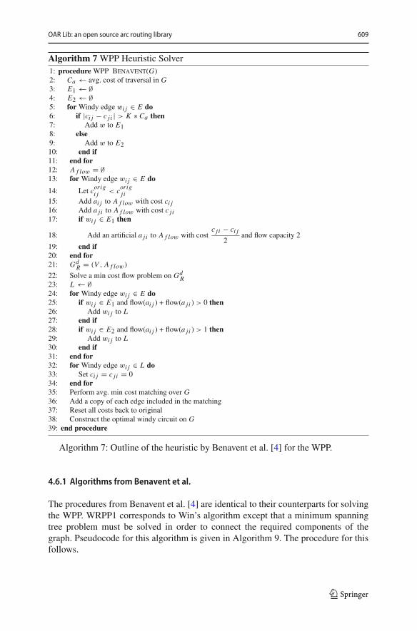
23: L ← ∅24: for Windy edge wi j ∈ E do25: if wi j ∈ E1 and flow(ai j ) + flow(a ji ) > 0 then26: Add wi j to L27: end if28: if wi j ∈ E2 and flow(ai j ) + flow(a ji ) > 1 then29: Add wi j to L30: end if31: end for32: for Windy edge wi j ∈ L do33: Set ci j = c ji = 034: end for35: Perform avg. min cost matching over G36: Add a copy of each edge included in the matching37: Reset all costs back to original38: Construct the optimal windy circuit on G39: end procedure
Algorithm 7: Outline of the heuristic by Benavent et al. [4] for the WPP.
4.6.1 Algorithms from Benavent et al.
The procedures from Benavent et al. [4] are identical to their counterparts for solvingthe WPP. WRPP1 corresponds to Win’s algorithm except that a minimum spanningtree problem must be solved in order to connect the required components of thegraph. Pseudocode for this algorithm is given in Algorithm 9. The procedure for thisfollows.
123

610 O. Lum et al.
Algorithm 8 DRPP Heuristic Solver1: procedure DRPP Christofides(G, AR )2: GR ← (V , AR)
3: C = C1,C2, . . . = connected components of GR4: VArb ← ∅5: AArb ← ∅6: for Component Ci ∈ C do7: Add vi to VArb8: end for9: for Arc ai j ∈ A do10: if vi ∈ Ci and v j ∈ C j and i �= j then11: Add ai j to AArb12: end if13: end for14: GArb = (VArb, AArb)
15: Solve a Minimum Spanning Arborescence (MSA) over GArb16: for Arc a ∈ MSA do17: Set a to required in G18: end for19: Solve a DCPP over G where supplies and demands given by GR20: Return Hierholzer(G)21: end procedure
Algorithm 8: Outline of Christofides’s heuristic [12] for the DRPP.
Algorithm 9WRPP Heuristic Solver1: procedure WRPP WIN WRPP1(G, ER )2: GR ← (V , ER)
3: C = C1,C2, . . . = connected components of GR4: VMST ← ∅5: EMST ← ∅6: for Component ci ∈ C do7: Add vi to VMST8: end for9: for Windy edge ei j ∈ E do10: if vi ∈ Ci and v j ∈ C j and i �= j then11: Add ei j to EMST with ci j = min (cavg(spi j ), cavg(sp ji ))12: end if13: end for14: GMST = (VMST , AMST )
15: Solve a Minimum Spanning Tree over GMST16: for Windy edge e ∈ MST do17: Set e to required in G18: end for19: Solve a WPP over G where degree is determined in GR20: Return Hierholzer(G)21: end procedure
Algorithm 9: Outline of Benavent et al.’s WRPP1 heuristic [4] for the WRPP.
123

OAR Lib: an open source arc routing library 611
1. Compute the connected components C1,C2,C3, . . . , of the graph GR .2. Construct the graph GC where the vertex set VC contains one vertex for each
connected component in GR .3. Complete GC by adding edges ei j with costs ci j = min (cavg(spi j ), cavg(sp ji )).4. Solve the minimum spanning tree (MST) problem on GC .5. If ei j was included in the MST, then set each edge in the shortest path represented
by ei j to be required.
5 Results
We present runtimes for the solvers in the library. All tests were performed on aMacBook Air (August 2012) with an i5-3427u processor. Figures 15, 16, 17 and 18give the runtimes in milliseconds (ms) for each of the solvers in the library. Figure 15shows results for the DCPP solver. Figure 16 shows results for the UCPP solver.Figure 17 compares the runtimes for the two MCPP solvers. Yaoyuenyong et al.’sheuristic is shown in red and it is clear that the improved objective values require largeruntimes. Figure 18 shows the runtimes for theWRPP solvers. Runtime was increasedby trying to modify the solution in anticipation of the optimal Euler circuit calculation.
For the UCPP and DCPP, we use a graph generator that randomly produces a graphwith a specified density, number of vertices, and connectedness (Boolean) as inputs.Most of the work involves producing the solution to the flow or matching probleminduced by the original graph. In order to solve the min cost matching problem, weuse the publicly available, efficient C++ implementation of the Blossom algorithmpresented by Kolmogorov [21]. To call this code from Java, we use a simple functionwrapper, with the Java Native Interface, to communicate cross-platform. This mayexplain why the UCPP solver’s performance on smaller problem instances does notmonotonically increase with problem size. For small instances, the overhead of callingthe function rather than the function itself dominates the runtime.
To validate the quality of the results, we replicated the objective function values ineach paper that introduced the methods using the same benchmark instances. For theDCPP and UCPP, the papers did not report computational results. However, becausethese are exact procedures, we compare the results of our solver to the objective func-tion values obtained by the IP formulation given earlier (Eqs. 1–4, and 5–7 for theDCPP and UCPP, respectively). The formulations were solved using Gurobi. For theMCPP, Yaoyuenyong et al. [32] presented a set of benchmark instances and compu-tational results for Frederickson’s heuristic and SAPH. We replicated these results.For the WPP and WRPP, Benavent et al. [4] did not present results on individualinstances. They instead reported deviation from the optimal solution averaged overthe set of Albaida–Madrigueras test instances [1]. These test instances are availablepublicly at http://www.uv.es/corberan/instancias.htm and were modeled on the streetnetwork of Albaida, Valencia. We reproduced this average deviation over the sameset of test instances. Benavent et al. [4] described an extension of Win’s heuristic forthe WPP that applies to the WRPP. For instances where all edges are required, thetwo heuristics are the same. Therefore, we use the averages reported by Benaventet al. for this procedure to validate Win’s heuristic. For the DRPP, we replicated the
123

612 O. Lum et al.
Fig. 15 Runtimes (ms) for our implementation of the DCPP exact solver to generate the optimal solution
Fig. 16 Runtimes (ms) for our implementation of the UCPP exact solver to generate the optimal solution
results presented by Campos and Savall [5] that gives a comparison of several DRPPheuristics.
In order to reproduce these results easily, a user should use the .jar file distributedwith the library as a command-line utility on the instances given on the GitHub page.One only needs to specify the instance file location and the appropriate solver. Theroute and the corresponding cost will be written to the output stream, where it may bewritten to a file, or used in another program. An example is given below.
java -Djava.library.path=/home/sharedLibs -jar ArcRoutingLibrary.jar3 test_instances/MCPP_Instances_Corberan/MA0532
123

OAR Lib: an open source arc routing library 613
Fig. 17 Runtimes (ms) for our implementation of Frederickson’s algorithm [14] in blue and Yaoyuenyonget al.’s algorithm [32] in red for the MCPP instances. Note that the time axis is scaled by 1e7, as indicatedby the label in the top left
Fig. 18 Runtimes (ms) for our implementation of the WRPP1 algorithm in blue and Benavent et al.’salgorithm [4] in red for the WRPP instances
This example shows the typical call structure when using the library as a standalonesolver. Thefirst argument following “/home/sharedLibs” contains the path to our linkedC++ libraries for solving the min cost matching and minimum spanning arbores-cence problems. The second argument “ArcRoutingLibrary.jar” contains the path tothe library. The third argument “3” indicates that we are calling Frederickson’s MCPPheuristic. The fourth argument “test_instances/MCPP_Instances_Corberan/MA0532”specifies the path to the problem instance to be solved. Full instructions are includedand distributed with the library.
123

614 O. Lum et al.
For the MCPP, we validate both heuristics using a set of instances given in [32].Instance characteristics and results for both MCPP heuristics on these instances aregiven in Table 4. These are small instances with 18 to 143 edges. Column three in thetable gives the sum of the costs of all links in the graph. We provide this informationbecause results in [32] are given as cost above this value, whereas we report the costof the tours produced by the two heuristics in columns four and six. To demonstratescaling, we run the heuristics on the set of Albaida–Madrigueras instances [1] forthe MCPP. These instances are grouped into sets of 24 with each set having a fixed|V | ∈ {500, 1000, 1500, 2000, 3000} for a total of 120 instances and varying |E | upto 9085. Results on these instances are given in Table 5.
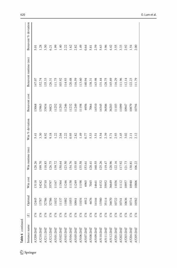
For the WPP and WRPP, validation and scaling were demonstrated using the setof 144 WRPP Albaida–Madrigueras instances [1]. There are two sets of instances.The instances beginning with “A” have 174 edges, while the instances beginningwith “M” have 316 edges. These instances have 83–230 required edges and 116–196vertices. Results on these instances are given in Table 6. Instance names are givenin the first column. The second column gives the number of edges in the instance.The third column gives the optimal objective function value. For all 144 instances,the optimal value is known. The costs of the tours produced by the two heuristics aregiven in columns four and seven. The runtimes given in columns five and eight showthat Win’s algorithm is slightly faster than the algorithm of Benavent et al. This isexpected, since the latter adds another min cost flow problem to the workflow. Allinstances are solved in under a second.
For the DRPP, validation and scaling of the solver were demonstrated using a setof instances given by Campos and Savall [5]. These instances have 211–801 arcs and80–240 vertices. The authors define an asymmetry index which they vary to create fiveversions of each instance. The asymmetry index measures how unbalanced vertices inthe graph are, with respect to the set of required arcs. Results on these instances aregiven in Table 7. In the first column, the name of the instance is given. The numbersafter the period give the level of asymmetry of the instance. 0 denotes a perfectlybalanced instance. 1_3 denotes an instance with an asymmetry index between 0 and1/3, 2_3 denotes an instance with an asymmetry index between 1/3 and 2/3, etc. Ingeneral, instances with more asymmetry result in more costly solutions. The secondcolumn gives the number of arcs in the graph. Campos and Savall report performanceabove the costs of the required arcs, so we include the sum of the required costs inthe third column. Solution cost is provided in the fourth column. The time requiredto solve each instance is given in the fifth column. As we expect, our heuristic runsquickly, taking no more than 2s on any instance.
All instances used to validate anddemonstrate scaling of the algorithms are providedin the distribution of the library.
We also include a suite of tests using the JUnit framework [29] that cover mostnon-trivial functions. JUnit is a test framework that gives Java coders the ability towrite a set of test routines. Tests contain several assert statements that compare theoutput of the test with an expected value. The test is said to fail if the assertion isfalse. For the code covered by the tests (logic paths executed by the test subroutines),running these tests whenever the code is modified allows the coder to isolate changesthat caused the tests to fail. Many popular integrated development environments have
123

OAR Lib: an open source arc routing library 615
Table4
Resultson
Yaoyu
enyo
ng[32]
MCPP
instances
Instance
name
|E|
Sum
oflin
kcosts
Frederickson
cost
Frederickson
runtim
e(m
s)SA
PHcost
SAPH
runtim
e(m
s)
A30
_1.nwk
5337
246
043
3.94
460
467.30
D21
_yut2.nw
k40
360
591
193.88
591
76.59
MHe116
a27.nw
k14
369
2282
9252
1.81
8185
1936
.27
MHe16a52
.nwk
6830
7648
1712
4.12
4763
89.45
MHe39a31
.nwk
7034
4141
2818
5.71
3983
311.88
MHe39a39
.nwk
7932
1644
7210
4.25
4281
114.45
MHe40a12
.nwk
5228
3634
1034
.30
3347
96.79
MHe44a49
.nwk
9340
2360
8813
4.08
6077
128.17
MHe61a24
.nwk
8536
7645
0777
.39
4380
176.80
MHe71a20
.nwk
9145
0055
9797
.10
5450
179.85
nobert.nwk
1882
106
9.13
106
4.94
123

616 O. Lum et al.
Table5
Resultson
Albaida-M
adrigu
eras
[1]MCPP
instances
Instance
name
|E|+
|A|
Sum
oflin
kcosts
Frederickson
cost
Frederickson
runtim
e(m
s)SA
PHcost
SAPH
runtim
e(m
s)
MA05
3282
242
0144
5398
8536
25.433
5330
4721
502.16
3
MA05
3584
042
9020
6645
5840
02.117
6513
0114
420.47
2
MA05
3784
044
5887
8346
0522
71.696
8332
9159
32.64
MA05
4210
2053
0070
6225
1421
24.674
6170
2339
652.69
6
MA05
4510
2853
0172
7139
6024
33.905
7004
7516
183.22
5
MA05
4710
3252
2771
8891
9321
85.48
8823
2716
593.16
7
MA05
5212
6066
5749
7517
7626
73.846
7424
1946
260.48
5
MA05
5512
6565
3945
8205
0131
11.764
8039
9830
416.00
3
MA05
5712
6566
7738
1043
202
2653
.704
1036
617
1547
8.12
3
MA05
6215
1281
3492
8779
0431
59.406
8740
0358
128.50
1
MA05
6515
0680
4312
9364
6239
92.17
9169
2032
991.99
MA05
6715
0077
6038
1071
000
3344
.306
1055
183
2977
7.63
5
MA10
3216
4185
1031
1079
588
7954
.625
1065
831
1410
00.175
MA10
3516
3883
6495
1311
379
9328
.021
1286
389
7107
3.26
1
MA10
3716
8388
2676
1606
722
1063
6.48
516
0351
245
960.10
1
MA10
4220
8810
8157
012
6396
811
631.22
712
5157
614
2854
.208
MA10
4520
6410
8477
714
8088
314
811.93
814
4545
914
0429
.206
MA10
4720
8011
3090
719
4766
613
255.38
1938
187
8372
3.34
5
123

OAR Lib: an open source arc routing library 617
Table5
continued
Instance
name
|E|+
|A|
Sum
oflin
kcosts
Frederickson
cost
Frederickson
runtim
e(m
s)SA
PHcost
SAPH
runtim
e(m
s)
MA10
5225
2512
8583
214
5030
415
410.43
114
3486
428
4123
.557
MA10
5525
4013
6643
216
8244
718
269.36
1655
700
1614
32.838
MA10
5725
3013
4602
420
8077
616
220.52
920
5917
091
387.61
1
MA10
6230
1815
9865
617
2806
020
116.43
117
2383
528
9136
.712
MA10
6530
0015
7581
618
2796
823
583.02
1790
324
2083
13.23
MA10
6730
2415
9041
622
3449
721
186.00
422
1436
015
5900
.705
MA15
3224
7813
1249
716
7827
625
507.69
616
5281
337
2595
.106
MA15
3524
9613
0589
120
5945
129
646.58
320
2851
826
6017
.933
MA15
3725
3213
4449
125
1163
029
174.21
825
0334
529
6601
.192
MA15
4230
9616
1958
419
2226
836
483.99
919
0097
157
8745
.267
MA15
4531
0816
1565
521
8804
039
233.94
421
3301
134
5207
.772
MA15
4730
8816
2355
728
9592
336
757.36
928
8127
824
2628
.114
MA15
5237
8519
7427
521
9870
444
052.37
321
9049
981
9899
.678
MA15
5538
2520
1856
124
9838
251
597.76
624
4155
169
2050
.547
MA15
5737
9019
5778
430
3791
047
971.28
930
1440
030
8167
.059
MA15
6245
1823
8278
525
7015
554
173.92
2565
713
1529
611.17
6
MA15
6545
0623
1706
527
0371
968
883.46
926
4313
693
7075
.213
MA15
6745
2424
0394
533
8656
864
471.66
433
4323
249
4812
.604
123

618 O. Lum et al.
Table5
continued
Instance
name
|E|+
|A|
Sum
oflin
kcosts
Frederickson
cost
Frederickson
runtim
e(m
s)SA
PHcost
SAPH
runtim
e(m
s)
MA20
3233
2717
5631
322
0769
354
048.37
521
7595
970
7610
.475
MA20
3533
1817
2549
227
1134
167
509.56
326
7780
150
4612
.035
MA20
3733
4817
4612
533
2446
461
708.70
933
1763
749
4510
.443
MA20
4241
8021
3784
024
9028
374
752.99
124
6044
219
2957
4.50
3
MA20
4541
3221
6043
429
5861
792
254.42
529
0058
587
5119
.183
MA20
4741
6021
7704
336
3934
080
810.96
536
1827
962
8471
.613
MA20
5250
5026
2972
629
4125
497
153.93
729
2246
316
8263
1.88
3
MA20
5550
8026
6664
233
1933
911
7452
.887
3249
532
1711
297.69
7
MA20
5750
6026
3800
540
0775
710
6299
.334
3972
850
8812
29.624
MA20
6260
3031
5093
734
1124
411
7584
.634
3402
556
3826
968.61
4
MA20
6560
3031
2096
136
4942
315
0099
.737
3576
530
1910
467.41
9
MA20
6760
3032
0210
346
9554
513
7507
.941
4655
446
1380
414.95
5
MA30
3249
8625
7130
732
5536
618
1139
.674
3200
848
3578
129.60
6
MA30
3550
2826
1772
139
6995
720
3138
.804
3916
247
2407
593.75
MA30
3749
3225
7721
151
5160
119
0500
.154
5133
545
1097
201.19
7
MA30
4261
7232
3528
338
0297
026
2318
.099
3756
400
3838
534.15
4
MA30
4562
3632
6938
944
3876
830
2357
.043
4337
870
3191
263.27
5
MA30
4762
7232
8218
056
3860
727
7490
.956
5602
380
2642
239.23
9
MA30
5276
0539
2209
743
8305
930
7036
.655
4342
995
8924
151.64
2
MA30
5575
9039
0138
148
9205
039
0438
.99
4786
701
5441
160.49
1
MA30
5775
8539
3031
460
3144
435
2528
.782
5983
597
2595
355.85
9
MA30
6290
4847
4639
951
3290
339
4298
.633
5119
449
1.33
E+07
MA30
6590
1846
8792
355
3082
648
1125
.591
5415
562
8809
387.90
9
MA30
6790
3646
9399
766
2159
644
6432
.316
6536
133
3438
866.03
123

OAR Lib: an open source arc routing library 619
Table6
Resultson
Albaida–M
adrigu
eras
[1]WRPP
instances
Instance
name
|E|
Optim
alWin
cost
Win
runtim
e(m
s)Win
%deviation
Benaventcost
Benaventruntim
e(m
s)Benavent%
deviation
A31
01.DAT
174
1042
410
497
123.92
0.70
1047
016
5.32
0.44
A31
02.DAT
174
1037
710
441
132.74
0.62
1042
214
1.38
0.43
A31
03.DAT
174
1042
710
615
173.05
1.80
1061
514
9.68
1.80
A31
04.DAT
174
1035
410
498
158.05
1.39
1054
114
0.98
1.81
A31
05.DAT
174
1033
210
474
150.08
1.37
1047
417
2.59
1.37
A31
06.DAT
174
1024
510
459
206.48
2.09
1042
714
1.46
1.78
A31
07.DAT
174
6531
6544
253.43
0.20
6634
254.68
1.58
A31
08.DAT
174
6568
6941
161.19
5.68
6941
169.39
5.68
A31
09.DAT
174
1313
213
826
186.07
5.28
1371
915
2.88
4.47
A31
10.DAT
174
1295
413
730
135.30
5.99
1388
614
8.15
7.19
A31
11.DAT
174
3095
733
678
172.39
8.79
3287
714
9.35
6.20
A31
12.DAT
174
3429
535
644
190.02
3.93
3551
616
5.67
3.56
A32
01.DAT
174
1008
310
464
169.84
3.78
1032
113
6.59
2.36
A32
02.DAT
174
1011
510
388
169.28
2.70
1038
812
2.28
2.70
A32
03.DAT
174
1007
710
295
125.63
2 .16
1026
812
8.53
1.90
A32
04.DAT
174
1000
110
326
138.23
3.25
1031
812
9.84
3.17
A32
05.DAT
174
1005
310
374
125.78
3.19
1037
412
2.68
3.19
A32
06.DAT
174
9915
1023
016
4.45
3.18
1020
715
5.65
2.95
A32
07.DAT
174
6873
7221
119.34
5.06
7212
135.14
4.93
A32
08.DAT
174
6813
7279
143.27
6.84
7268
152.29
6.68
123
620 O. Lum et al.
Table6
continued
Instance
name
|E|
Optim
alWin
cost
Win
runtim
e(m
s)Win
%deviation
Benaventcost
Benaventruntim
e(m
s)Benavent%
deviation
A32
09.DAT
174
1244
513
118
128.26
5.41
1306
814
7.07
5.01
A32
10.DAT
174
1378
714
242
199.70
3.30
1396
315
2.74
1.28
A32
11.DAT
174
3278
635
710
118.85
8.92
3393
413
5.33
3.50
A32
12.DAT
174
3278
635
797
126.75
9.18
3482
112
6.31
6.21
A51
01.DAT
174
1103
211
167
139.72
1.22
1125
211
1.75
1.99
A51
02.DAT
174
1113
711
364
150.64
2.04
1129
310
3.92
1.40
A51
03.DAT
174
1100
211
246
123.50
2.22
1124
611
4.93
2.22
A51
04.DAT
174
1105
311
158
154.76
0.95
1123
212
0.48
1.62
A51
05.DAT
174
1094
111
249
135.95
2.82
1124
911
6.59
2.82
A51
06.DAT
174
1103
411
198
135.58
1.49
1119
811
3.60
1.49
A51
07.DAT
174
6912
6965
153.61
0.77
6956
140.94
0.64
A51
08.DAT
174
6676
7045
128.41
5.53
7064
138.31
5.81
A51
09.DAT
174
1414
414
641
160.55
3.51
1451
014
3.98
2.59
A51
10.DAT
174
1358
014
332
125.26
5.54
1434
513
1.44
5.63
A51
11.DAT
174
3511
435
952
119.47
2 .39
3650
612
8.75
3.96
A51
12.DAT
174
3467
036
649
128.96
5.71
3620
314
5.69
4.42
A52
01.DAT
174
1072
211
036
122.16
2.93
1110
311
6.29
3.55
A52
02.DAT
174
1074
111
112
117.92
3.45
1109
911
1.96
3.33
A52
03.DAT
174
1063
610
957
121.73
3.02
1094
711
2.14
2.92
A52
04.DAT
174
1071
410
940
130.81
2.11
1087
912
2.23
1.54
A52
05.DAT
174
1058
210
806
106.22
2.12
1079
411
1.79
2.00
123

OAR Lib: an open source arc routing library 621
Table6
continued
Instance
name
|E|
Optim
alWin
cost
Win
runtim
e(m
s)Win
%deviation
Benaventcost
Benaventruntim
e(m
s)Benavent%
deviation
A52
06.DAT
174
1060
010
988
115.90
3.66
1097
112
6.48
3.50
A52
07.DAT
174
6815
7166
117.05
5.15
7232
156.81
6.12
A52
08.DAT
174
7038
7277
103.08
3.40
7282
145.69
3.47
A52
09.DAT
174
1290
113
412
107.04
3.96
1322
513
4.10
2.51
A52
10.DAT
174
1413
114
563
99.98
3.06
1459
513
6.06
3.28
A52
11.DAT
174
3573
936
069
102.30
0.92
3623
712
5.14
1.39
A52
12.DAT
174
3579
736
774
102.49
2.73
3697
213
6.65
3.28
A71
01.DAT
174
1201
512
015
98.71
0.00
1201
510
9.91
0.00
A71
02.DAT
174
1205
712
057
91.68
0.00
1205
710
3.36
0.00
A71
03.DAT
174
1193
611
944
93.11
0.07
1194
410
3.34
0.07
A71
04.DAT
174
1198
811
992
96.15
0.03
1199
110
7.43
0.03
A71
05.DAT
174
1182
911
860
95.52
0.26
1186
010
3.81
0.26
A71
06.DAT
174
1178
011
780
106.14
0.00
1178
011
1.76
0.00
A71
07.DAT
174
7271
7436
92.35
2.27
7393
124.42
1.68
A71
08.DAT
174
8080
8156
98.06
0 .94
8160
125.43
0.99
A71
09.DAT
174
1608
616
296
96.90
1.31
1629
611
5.52
1.31
A71
10.DAT
174
1501
815
484
91.97
3.10
1541
712
9.04
2.66
A71
11.DAT
174
3490
336
801
99.00
5.44
3700
912
8.91
6.03
A71
12.DAT
174
3766
737
679
104.64
0.03
3782
912
8.54
0.43
A72
01.DAT
174
1098
511
017
141.26
0.29
1101
796
.49
0.29
123

622 O. Lum et al.
Table6
continued
Instance
name
|E|
Optim
alWin
cost
Win
runtim
e(m
s)Win
%deviation
Benaventcost
Benaventruntim
e(m
s)Benavent%
deviation
A72
02.DAT
174
1097
010
995
116.87
0.23
1099
110
4.29
0.19
A72
03.DAT
174
1089
710
916
93.81
0.17
1089
795
.33
0.00
A72
04.DAT
174
1099
511
032
95.06
0.34
1101
210
0.41
0.15
A72
05.DAT
174
1088
810
926
105.68
0.35
1092
610
2.52
0.35
A72
06.DAT
174
1094
910
997
103.48
0.44
1099
711
5.78
0.44
A72
07.DAT
174
6757
6894
100.87
2.03
6850
139.33
1.38
A72
08.DAT
174
6902
7053
100.45
2.19
6962
132.85
0.87
A72
09.DAT
174
1424
614
709
103.68
3.25
1460
114
0.18
2.49
A72
10.DAT
174
1369
113
963
108.92
1.99
1380
915
4.61
0.86
A72
11.DAT
174
3707
138
785
103.13
4.62
3878
513
7.88
4.62
A72
12.DAT
174
3456
935
812
104.43
3.60
3581
214
2.01
3.60
M31
01.DAT
316
1740
717
782
376.37
2.15
1775
143
4.17
1.98
M31
02.DAT
316
1736
617
967
390.53
3.46
1789
143
2.84
3.02
M31
03.DAT
316
1732
517
641
499.66
1.82
1757
157
6.32
1.42
M31
04.DAT
316
1736
217
978
354.45
3 .55
1797
840
3.40
3.55
M31
05.DAT
316
1731
817
829
352.65
2.95
1776
640
8.01
2.59
M31
06.DAT
316
1711
817
537
356.65
2.45
1746
343
6.53
2.02
M31
07.DAT
316
9485
9900
342.54
4.38
9785
573.76
3.16
M31
08.DAT
316
1051
411
236
368.90
6.87
1116
446
3.80
6.18
M31
09.DAT
316
1945
220
341
333.80
4.57
2072
746
3.06
6.55
M31
10.DAT
316
1950
620
412
412.21
4.64
2076
946
0.16
6.47
123

OAR Lib: an open source arc routing library 623
Table6
continued
Instance
name
|E|
Optim
alWin
cost
Win
runtim
e(m
s)Win
%deviation
Benaventcost
Benaventruntim
e(m
s)Benavent%
deviation
M31
11.DAT
316
5070
955
288
434.60
9.03
5415
746
6.30
6.80
M31
12.DAT
316
4968
752
511
615.87
5.68
5253
551
2.16
5.73
M32
01.DAT
316
1723
018
176
490.12
5.49
1821
840
3.65
5.73
M32
02.DAT
316
1723
718
001
444.11
4.43
1786
542
2.44
3.64
M32
03.DAT
316
1716
818
140
609.95
5.66
1806
157
2.54
5.20
M32
04.DAT
316
1706
917
658
434.20
3.45
1764
043
3.37
3.35
M32
05.DAT
316
1732
817
987
584.90
3.80
1795
256
0.02
3.60
M32
06.DAT
316
1700
017
772
575.38
4.54
1755
154
6.66
3.24
M32
07.DAT
316
1028
411
583
381.02
12.63
1136
147
1.95
10.47
M32
08.DAT
316
9694
1059
848
7.53
9.33
1063
249
0.92
9.68
M32
09.DAT
316
2036
021
779
583.69
6.97
2201
265
4.53
8.11
M32
10.DAT
316
2032
821
971
377.47
8.08
2155
744
6.03
6.05
M32
11.DAT
316
5273
457
335
383.93
8.72
5695
847
5.05
8.01
M32
12.DAT
316
5057
654
492
396.83
7.74
5366
647
5.33
6.11
M51
01.DAT
316
1851
218
777
354.11
1 .43
1881
534
8.82
1.64
M51
02.DAT
316
1855
918
799
394.97
1.29
1879
940
2.69
1.29
M51
03.DAT
316
1827
018
425
379.22
0.85
1849
437
3.07
1.23
M51
04.DAT
316
1844
518
811
347.36
1.98
1881
138
6.60
1.98
M51
05.DAT
316
1842
818
795
343.09
1.99
1872
339
4.51
1.60
M51
06.DAT
316
1850
018
784
331.33
1.54
1865
738
0.68
0.85
123

624 O. Lum et al.
Table6
continued
Instance
name
|E|
Optim
alWin
cost
Win
runtim
e(m
s)Win
%deviation
Benaventcost
Benaventruntim
e(m
s)Benavent%
deviation
M51
07.DAT
316
1063
111
224
333.57
5.58
1100
042
1.48
3.47
M51
08.DAT
316
1141
012
232
325.33
7.20
1203
147
6.93
5.44
M51
09.DAT
316
2130
223
017
336.82
8.05
2268
142
5.47
6.47
M51
10.DAT
316
2358
924
533
340.95
4.00
2427
541
7.68
2.91
M51
11.DAT
316
5246
955
590
340.42
5.95
5681
257
0.52
8.28
M51
12.DAT
316
5416
256
045
335.03
3.48
5664
743
2.61
4.59
M52
01.DAT
316
1856
118
852
330.44
1.57
1882
035
2.06
1.40
M52
02.DAT
316
1855
318
929
322.23
2.03
1889
635
3.37
1.85
M52
03.DAT
316
1854
618
736
480.10
1.02
1873
650
1.82
1.02
M52
04.DAT
316
1848
918
812
301.22
1.75
1877
935
3.44
1.57
M52
05.DAT
316
1847
018
737
318.87
1.45
1868
535
6.91
1.16
M52
06.DAT
316
1849
718
942
298.78
2.41
1901
236
0.81
2.78
M52
07.DAT
316
1140
111
788
368.77
3.39
1178
046
8.97
3.32
M52
08.DAT
316
1106
411
736
355.95
6.07
1164
543
7.60
5.25
M52
09.DAT
316
2233
023
204
369.91
3 .91
2316
044
5.60
3.72
M52
10.DAT
316
2155
422
233
358.67
3.15
2218
044
7.39
2.90
M52
11.DAT
316
5305
655
684
322.27
4.95
5483
441
0.42
3.35
M52
12.DAT
316
5301
954
401
340.75
2.61
5440
144
6.32
2.61
M71
01.DAT
316
2149
521
506
318.14
0.05
2150
633
3.91
0.05
M71
02.DAT
316
2149
521
495
331.02
0.00
2149
534
7.13
0.00
M71
03.DAT
316
2150
021
500
322.99
0.00
2150
037
7.91
0.00
123

OAR Lib: an open source arc routing library 625
Table6
continued
Instance
name
|E|
Optim
alWin
cost
Win
runtim
e(m
s)Win
%deviation
Benaventcost
Benaventruntim
e(m
s)Benavent%
deviation
M71
04.DAT
316
2152
121
521
309.93
0.00
2152
134
0.35
0.00
M71
05.DAT
316
2138
521
385
336.37
0.00
2138
534
7.80
0.00
M71
06.DAT
316
2138
521
385
345.21
0.00
2138
535
1.32
0.00
M71
07.DAT
316
1317
913
681
341.09
3.81
1367
941
3.23
3.79
M71
08.DAT
316
1257
812
766
328.76
1.49
1276
642
5.15
1.49
M71
09.DAT
316
2487
225
119
306.01
0.99
2508
241
8.05
0.84
M71
10.DAT
316
2606
726
669
319.56
2.31
2663
442
9.80
2.18
M71
11.DAT
316
6469
465
597
301.63
1.40
6559
742
4.47
1.40
M71
12.DAT
316
6207
163
557
307.54
2.39
6327
243
4.80
1.93
M72
01.DAT
316
2181
521
815
351.30
0.00
2181
535
9.03
0.00
M72
02.DAT
316
2184
421
898
370.65
0.25
2184
435
1.65
0.00
M72
03.DAT
316
2161
221
641
320.66
0.13
2164
138
2.76
0.13
M72
04.DAT
316
2167
121
732
310.99
0.28
2175
034
2.75
0.36
M72
05.DAT
316
2165
221
668
331.38
0.07
2172
935
9.27
0.36
M72
06.DAT
316
2160
721
608
310.78
0 .00
2160
835
0.40
0.00
m72
07.DAT
316
1284
013
089
321.30
1.94
1307
343
0.31
1.81
m72
08.DAT
316
1241
912
679
306.60
2.09
1272
343
1.32
2.45
m72
09.DAT
316
2509
325
940
316.88
3.38
2594
043
7.96
3.38
m72
10.DAT
316
2467
325
471
306.94
3.23
2533
141
4.57
2.67
m72
11.DAT
316
6143
763
699
292.74
3.68
6341
041
4.44
3.21
m72
12.DAT
316
6408
866
092
321.51
3.13
6630
244
0.28
3.45
123

626 O. Lum et al.
Table 7 Results on Campos and Savall [5] DRPP instances
Instance Name |A| AR cost Christofides et al.Cost Christofides et al. Runtime (ms)
160-20-1.0 440 10245 16339 1653.28
160-20-1.1 511 6330 18809 2764.27
160-20-1.1_3 452 12750 20870 508.11
160-20-1.2_3 452 7985 19144 629.04
160-20-1.3_3 511 8490 18924 530.39
160-20-2.0 437 9676 16302 257.71
160-20-2.1 503 6495 19340 487.78
160-20-2.1_3 464 12449 21442 394.64
160-20-2.2_3 464 10453 22358 540.27
160-20-2.3_3 500 6858 20094 536.23
160-20-3.0 471 11477 18129 207.96
160-20-3.1 539 6771 18778 592.41
160-20-3.1_3 486 12368 20764 347.23
160-20-3.2_3 486 11383 20311 471.24
160-20-3.3_3 539 7425 20296 627.58
160-20-4.0 468 10952 15883 153.84
160-20-4.1 530 6527 18887 547.64
160-20-4.1_3 485 11299 18805 405.06
160-20-4.2_3 486 10235 21173 467.60
160-20-4.3_3 530 8366 21107 501.78
240-30-1.0 667 13792 22857 699.03
240-30-1.1 763 9915 30443 1785.91
240-30-1.1_3 703 19696 34592 1317.85
240-30-1.2_3 703 15668 29585 1480.09
240-30-1.3_3 763 10592 28138 1453.23
240-30-2.0 693 16925 26564 632.77
240-30-2.1 795 9405 29045 1934.13
240-30-2.1_3 701 15798 26782 797.67
240-30-2.2_3 711 14294 27179 1393.55
240-30-2.3_3 796 11327 30430 1810.78
240-30-3.0 697 17119 26121 607.27
240-30-3.1 801 10416 30232 1914.48
240-30-3.1_3 705 17481 27920 1103.76
240-30-3.2_3 716 15647 26813 1328.90
240-30-3.3_3 801 11707 31130 1993.74
240-30-4.0 699 15768 25125 665.03
240-30-4.1 792 8915 26406 1899.80
240-30-4.1_3 708 15234 26707 1164.95
240-30-4.2_3 716 12716 25540 1384.28
240-30-4.3_3 792 10259 28377 1589.94
123

OAR Lib: an open source arc routing library 627
Table 7 continued
Instance Name |A| AR cost Christofides et al.Cost Christofides et al. Runtime (ms)
P80-10-1.0 211 5950 8844 24.54
P80-10-1.1 249 3798 10550 85.71
P80-10-1.1_3 224 7585 11508 50.40
P80-10-1.2_3 224 6471 11780 52.45
P80-10-1.3_3 249 4335 12983 80.82
P80-10-2.0 217 4835 7677 22.27
P80-10-2.1 247 2436 8719 52.00
P80-10-2.1_3 228 7165 10845 38.42
P80-10-2.2_3 226 6353 11276 46.84
P80-10-2.3_3 248 3273 8921 64.80
P80-10-3.0 213 4857 7817 23.95
P80-10-3.1 240 2981 8894 64.44
P80-10-3.1_3 226 6649 12542 51.39
P80-10-3.2_3 226 4590 8882 50.87
P80-10-3.3_3 240 3164 8754 44.39
P80-10-4.0 240 5785 8396 25.63
P80-10-4.1 277 3646 8540 76.49
P80-10-4.1_3 252 7730 11614 48.73
P80-10-4.2_3 252 6986 10993 62.88
P80-10-4.3_3 277 4192 8524 70.42
plug-ins that allow for tests written using JUnit to be run for continuous integration,automatically alerting the coder as soon as the violating change is made without amanual run of the tests. These tests give potential contributers an easy way to validatechanges without having to be familiar with parts of the code that they did not write.Users of the library may also examine these tests as additional documentation of theintended use of each function.
6 Conclusions
We implemented a suite of solvers for well-known arc routing problems and pre-sented computational results on several sets of benchmark instances. For the UCPPand DCPP, we provided exact solvers. For the MCPP, WPP, DRPP, and WRPP, weprovided heuristic solvers. We implemented and discussed the underlying code archi-tecture. We demonstrated its flexibility in accommodating a variety of graph typesand problem features. The code is released under the MIT License and is availableat github.com/olibear/ArcRoutingLibrary. We have used the framework provided bythe library to develop heuristics for other problems. In [6,24], we extend the libraryto develop a heuristic for a problem with multiple vehicles and a min-max objectivefunction. In [25], we extend the library to solve a variant of theWRPP with alternative
123

628 O. Lum et al.
service options.We plan to support the library in the future using GitHub’s built-in bugreporting and tracking features to address requests and issues. In addition, we expectto update the library with additional local search procedures, objective functions, andproblem definitions based on the demand from potential users. In future work, hetero-geneous fleets, multi-modal transportation, and multiple depots should be integratedto allow for richer problems to be modeled.
References
1. Arc Routing Problems: Data Instances. http://www.uv.es/corberan/instancias.htm2. Ahr, D., Reinelt, G.: New heuristics and lower bounds for the min-max k-Chinese postman problem.
Algorithms-ESA 2002, pp. 64–74. Springer, Berlin (2002)3. Bastian,M., Heymann, S., Jacomy,M.: Gephi: an open source software for exploring andmanipulating
networks. ICWSM 8, 361–362 (2009)4. Benavent, E., Corberán, A., Piñana, E., Plana, I., Sanchis, J.M.: New heuristic algorithms for the windy
rural postman problem. Comput. Oper. Res. 32(12), 3111–3128 (2005)5. Campos, V., Savall, J.V.: A computational study of several heuristics for the DRPP. Comput. Optim.
Appl. 4(1), 67–77 (1995)6. Corberán, A., Golden, B., Lum, O., Plana, I., Sanchis, J.: Aesthetic considerations for the min-max k
windy rural postman problem. Networks 70(3), 216–232 (2017)7. Derigs, U.: Optimization and Operations Research. Eolss Publishers Company Limited, New York
(2009)8. Dijkstra, E.W.: A note on two problems in connexion with graphs. Numer. Math. 1(1), 269–271 (1959)9. Dussault, B., Golden, B., Groër, C.,Wasil, E.: Plowingwith precedence: a variant of the windy postman
problem. Comput. Oper. Res. 40(4), 1047–1059 (2013)10. Edmonds, J., Johnson, E.L.: Matching, Euler tours and the Chinese postman. Math. Program. 5(1),
88–124 (1973)11. Eiselt, H.A., Gendreau, M., Laporte, G.: Arc routing problems, part I: the Chinese postman problem.
Oper. Res. 43(2), 231–242 (1995)12. Eiselt, H.A., Gendreau, M., Laporte, G.: Arc routing problems, part II: the rural postman problem.
Oper. Res. 43(3), 399–414 (1995)13. Floyd, R.W.: Algorithm 97: shortest path. Commun. ACM 5(6), 345 (1962)14. Frederickson, G.N.: Approximation algorithms for some postman problems. J. ACM 26(3), 538–554
(1979)15. GNU Trove library. http://trove.starlight-systems.com/16. Groër, C., Golden, B., Wasil, E.: A library of local search heuristics for the vehicle routing problem.
Math. Program. Comput. 2(2), 79–101 (2010)17. Grötschel, M., Win, Z.: A cutting plane algorithm for the windy postman problem. Math. Program.
55(1–3), 339–358 (1992)18. Haklay, M., Weber, P.: Openstreetmap: user-generated street maps. IEEE Pervasive Comput. 7(4),
12–18 (2008)19. Hierholzer, C., Wiener, C.: Über die Möglichkeit, einen Linienzug ohne Wiederholung und ohne
Unterbrechung zu umfahren. Math. Ann. 6(1), 30–32 (1873)20. Karypis, G., Kumar, V.: A fast and high quality multilevel scheme for partitioning irregular graphs.
SIAM J. Sci. Comput. 20(1), 359–392 (1998)21. Kolmogorov, V., Blossom, V.: A new implementation of a minimum cost perfect matching algorithm.
Math. Program. Comput. 1(1), 43–67 (2009)22. Lau, H.T.: A Java Library of Graph Algorithms and Optimization. CRC Press, London (2010)23. Letchford, A.N., Reinelt, G., Theis, D.O.: A faster exact separation algorithm for blossom inequalities.
In: Integer Programming and Combinatorial Optimization, pp. 196–205. Springer, Berlin (2004)24. Lum, O., Cerrone, C., Golden, B., Wasil, E.: Partitioning a street network into compact, balanced, and
visually appealing routes. Networks 69(3), 290–303 (2016)25. Lum, O., Zhang, R., Golden, B., Wasil, E.: A hybrid heuristic for the windy rural postman problem
with time-dependent zigzag options. Comput. Oper. Res. 88, 247–257 (2017)
123

OAR Lib: an open source arc routing library 629
26. Minimum cost flow tutorial. http://community.topcoder.com/tc?module=Static&d1=tutorials&d2=minimumCostFlow2
27. Padberg, M.W., Rao, M.R.: Odd minimum cut-sets and b-matchings. Math. Oper. Res. 7(1), 67–80(1982)
28. Prim, R.C.: Shortest connection networks and some generalizations. Bell Syst. Tech. J. 36(6), 1389–1401 (1957)
29. Tahchiev, P., Leme, F., Massol, V., Gregory, G.: JUnit in Action. Manning Publications Co, New York(2010)
30. Thimbleby, H.: The directed Chinese postman problem. Softw. Pract. Exp. 33(11), 1081–1096 (2003)31. Win, Z.: On the windy postman problem on Eulerian graphs. Math. Program. 44(1–3), 97–112 (1989)32. Yaoyuenyong, K., Charnsethikul, P., Chankong, V.: A heuristic algorithm for the mixed Chinese post-
man problem. Optim. Eng. 3(2), 157–187 (2002)
Publisher’s Note Springer Nature remains neutral with regard to jurisdictional claims in published mapsand institutional affiliations.
123