object classification from randomized eeg trials
TRANSCRIPT
Object classification from randomized EEG trials
Hamad Ahmed Ronnie B. Wilbur Hari M. Bharadwaj Jeffrey Mark Siskind
Purdue University, West Lafayette, IN, 47907
{ahmed90,wilbur,hbharadwaj,qobi}@purdue.edu
Abstract
New results suggest strong limits to the feasibility of ob-
ject classification from human brain activity evoked by im-
age stimuli, as measured through EEG. Considerable prior
work suffers from a confound between the stimulus class
and the time since the start of the experiment. A prior at-
tempt to avoid this confound using randomized trials was
unable to achieve results above chance in a statistically sig-
nificant fashion when the data sets were of the same size as
the original experiments. Here, we attempt object classifi-
cation from EEG using an array of methods that are rep-
resentative of the state-of-the-art, with a far larger (20×)
dataset of randomized EEG trials, 1,000 stimulus presenta-
tions of each of forty classes, all from a single subject. To
our knowledge, this is the largest such EEG data-collection
effort from a single subject and is at the bounds of feasi-
bility. We obtain classification accuracy that is marginally
above chance and above chance in a statistically significant
fashion, and further assess how accuracy depends on the
classifier used, the amount of training data used, and the
number of classes. Reaching the limits of data collection
with only marginally above-chance performance suggests
that the prevailing literature substantially exaggerates the
feasibility of object classification from EEG.
1. Introduction
There has been considerable recent interest in applying
deep learning to electroencephalography (EEG). Two re-
cent survey papers [7, 33] collectively contain 372 refer-
ences. Much of this work attempts to classify human brain
activity evoked from visual stimuli. A recent CVPR oral
[35] claims to decode one of forty object classes when sub-
jects view images from ImageNet [9] with 82.9% accu-
racy. Considerable follow-on work uses the same dataset
[5, 10, 11, 12, 13, 15, 16, 17, 19, 21, 25, 26, 27, 28, 29,
30, 43, 46, 47, 48, 49], often claiming even higher accu-
racy. Li et al. [22] demonstrate that this classification ac-
curacy is severely overinflated due to flawed experimental
design. All stimuli of the same class were presented to sub-
jects as a single block (Fig. 1a). Further, training and test
samples were taken from the same block. Because all EEG
data contain long-term temporal correlations that are unre-
lated to stimulus processing and their design confounded
block-effects with class label, Spampinato et al. [35] were
classifying these long-term temporal patterns, not the stim-
ulus class. Because the training and test samples were taken
in close temporal proximity from the same block, the tem-
poral correlations in the EEG introduced label leakage be-
tween the training and test data sets. When the experiment
of Spampinato et al. [35] is repeated with randomized trials,
where stimuli of different classes are randomly intermixed,
classification accuracy drops to chance [22].
Another recent paper [8] attempts to remedy the short-
comings of a block design by recording two different ses-
sions for the same subject, each organized as a block de-
sign, one to be used as training data and one to be used as
test data. However, both sessions used the same stimulus
presentation order (Fig. 1b). Li et al. [22] demonstrate that
classification accuracy can even be severely inflated with
such a cross-session design that employs the same stim-
ulus presentation order in both sessions due to the same
long-term transients that are unrelated to stimulus process-
ing. While an analysis of training and test sets coming from
different sessions with the same stimulus presentation or-
der yields lower accuracy than an analysis where they come
from the same session, accuracy drops to chance when the
two sessions have different stimulus presentation order.
All this prior work is fundamentally flawed due to im-
proper experimental design. Essentially, the EEG signal en-
codes a clock and any experimental design where stimulus
class correlates with time since beginning of experiment al-
lows classifying the clock instead of the stimuli. This means
that all data collected in this fashion is irreparably contami-
nated.
Li et al. [22] attempted to replicate the experiment of
Spampinato et al. [35] six times with nine different classi-
fiers, including the LSTM employed by them, with random-
ized trials (Fig. 1c) instead of a block design. All attempts
failed, yielding chance performance.
Given that considerable prior work suffers from this
3845
(a)
class 1 im
age 3
class 1 im
age 4
class 1 im
age 2
class 2 im
age 1
class 2 im
age 2
class 2 im
age 3
class 2 im
age 4
training test training test
class 1 im
age 1
(b)
class 1 im
age 3
class 1 im
age 4
class 1 im
age 2
class 2 im
age 1
class 2 im
age 2
class 2 im
age 3
class 2 im
age 4
later class 1 im
age 2
class 1 im
age 4
class 1 im
age 3
class 2 im
age 1
class 2 im
age 2
class 2 im
age 3
class 2 im
age 4
training test
class 1 im
age 1
class 1 im
age 1
(c)
class 19 im
age 23 training
class 14 im
age 6 training
class 3 im
age 14 test
class 1 im
age 4 training
class 29 im
age 11 test
class 14 im
age 3 training
class 7 im
age 15 test
class 27 im
age 4 training
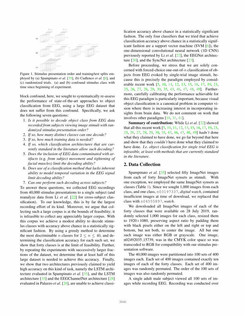
Figure 1. Stimulus presentation order and training/test splits em-
ployed by (a) Spampinato et al. [35], (b) Cudlenco et al. [8], and
(c) randomized trials. (a) and (b) confound stimulus class with
time since beginning of experiment.
block confound, here, we sought to systematically re-assess
the performance of state-of-the-art approaches to object
classification from EEG, using a large EEG dataset that
does not suffer from this confound. Specifically, we ask
the following seven questions:
1. Is it possible to decode object class from EEG data
recorded from subjects viewing image stimuli with ran-
domized stimulus presentation order?
2. If so, how many distinct classes can one decode?
3. If so, how much training data is needed?
4. If so, which classification architectures that are cur-
rently standard in the literature allow such decoding?
5. Does the inclusion of EEG data contaminated with ar-
tifacts (e.g. from subject movement and tightening of
facial muscles) limit the decoding ability?
6. Does use of a classification method that lacks inherent
ability to model temporal variation in the EEG signal
limit decoding ability?
7. Can one perform such decoding across subjects?
To answer these questions, we collected EEG recordings
from 40,000 stimulus presentations to a single subject (and
reanalyze data from Li et al. [22] for cross-subject clas-
sification). To our knowledge, this is by far the largest
recording effort of its kind. Moreover, we argue that col-
lecting such a large corpus is at the bounds of feasibility; it
is infeasible to collect any appreciably larger corpus. With
this corpus we achieve a modest ability to decode stimu-
lus classes with accuracy above chance in a statistically sig-
nificant fashion. By using a greedy method to determine
the most discriminable n classes for 2 ≤ n ≤ 40, and de-
termining the classification accuracy for each such set, we
show that forty classes is at the limit of feasibility. Further,
by repeating the experiments with successively larger frac-
tions of the dataset, we determine that at least half of this
large dataset is needed to achieve this accuracy. Finally,
we show that two architectures previously claimed to yield
high accuracy on this kind of task, namely the LSTM archi-
tecture evaluated in Spampinato et al. [35], and the LSTM
architecture [35] and the EEGChannelNet architecture [28]
evaluated in Palazzo et al. [28], are unable to achieve classi-
fication accuracy above chance in a statistically significant
fashion. The only four classifiers that we tried that achieve
classification accuracy above chance in a statistically signif-
icant fashion are a support vector machine (SVM [6]), the
one-dimensional convolutional neural network (1D CNN)
previously reported by Li et al. [22], the EEGNet architec-
ture [20], and the SyncNet architecture [23].
Before proceeding, we stress that we are solely con-
cerned with forced-choice one-out-of-n classification of ob-
jects from EEG evoked by single-trial image stimuli, be-
cause this is precisely the paradigm employed by consid-
erable recent work [5, 10, 11, 12, 13, 15, 16, 17, 19, 21,
25, 26, 27, 28, 29, 30, 35, 43, 46, 47, 48, 49]. Further-
more, carefully calibrating the performance achievable for
this EEG paradigm is particularly important, because visual
object classification is a canonical problem in computer vi-
sion where there is increasing interest in incorporating in-
sights from brain data. We do not comment on work that
involves other paradigms [18, 31, 41].
Summary of contribution: While Li et al. [22] showed
that all this recent work [5, 10, 11, 12, 13, 15, 16, 17, 19, 21,
25, 26, 27, 28, 29, 30, 35, 43, 46, 47, 48, 49] hadn’t done
what they claimed to have done, we go far beyond that here
and show that they couldn’t have done what they claimed to
have done. I.e. object classification for single trial EEG is
infeasible, at least with methods that are currently standard
in the literature.
2. Data Collection
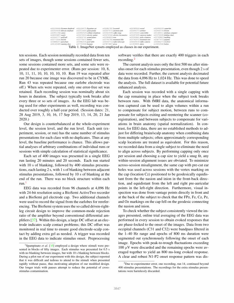
Spampinato et al. [35] selected fifty ImageNet images
from each of forty ImageNet synsets as stimuli. With
one exception, we employed the same ImageNet synsets as
classes (Table 1). Since we sought 1,000 images from each
class, and one class, n03197337, digital watch, contained
insufficient images at time of download, we replaced that
class with n04555897, watch.
We downloaded all ImageNet images of each of the
forty classes that were available on 28 July 2019, ran-
domly selected 1,000 images for each class, resized them
to 1920×1080, preserving aspect ratio by padding them
with black pixels either on the left and right or top and
bottom, but not both, to center the image. All but one
such image was either RGB or grayscale. One image,
n02492035 15739, was in the CMYK color space so was
transcoded to RGB for compatibility with our stimulus pre-
sentation software.
The 40,000 images were partitioned into 100 sets of 400
images each. Each set of 400 images contained exactly ten
images of each of the forty classes. Each set of 400 im-
ages was randomly permuted. The order of the 100 sets of
images was also randomly permuted.
A single adult male subject viewed all 100 sets of im-
ages while recording EEG. Recording was conducted over
3846
n02106662 German shepherd n02124075 Egyptian cat n02281787 lycaenid n02389026 sorrel n02492035 capuchin
n02504458 African elephant n02510455 giant panda n02607072 anemone fish n02690373 airliner n02906734 broom
n02951358 canoe n02992529 cellular telephone n03063599 coffee mug n03100240 convertible n03180011 desktop computer
n04555897 watch n03272010 electric guitar n03272562 electric locomotive n03297495 espresso maker n03376595 folding chair
n03445777 golf ball n03452741 grand piano n03584829 iron n03590841 jack-o-lantern n03709823 mailbag
n03773504 missile n03775071 mitten n03792782 mountain bike n03792972 mountain tent n03877472 pajama
n03888257 parachute n03982430 pool table n04044716 radio telescope n04069434 reflex camera n04086273 revolver
n04120489 running shoe n07753592 banana n07873807 pizza n11939491 daisy n13054560 bolete
Table 1. ImageNet synsets employed as classes in our experiment.
ten sessions. Each session nominally recorded data from ten
sets of images, though some sessions contained fewer sets,
some sessions contained more sets, and some sets were re-
peated due to experimenter error. (Runs per session: 10, 8,
10, 11, 11, 10, 10, 10, 10, 10. Run 19 was repeated after
run 20 because one image was discovered to be in CYMK.
Run 43 was repeated because one earlobe electrode was
off.) When sets were repeated, only one error-free set was
retained. Each recording session was nominally about six
hours in duration. The subject typically took breaks after
every three or so sets of images. As the EEG lab was be-
ing used for other experiments as well, recording was con-
ducted over roughly a half-year period. (Session dates: 21,
28 Aug 2019, 3, 10, 16, 17 Sep 2019, 13, 14, 20, 21 Jan
2020.)
Our design is counterbalanced at the whole-experiment
level, the session level, and the run level. Each unit (ex-
periment, session, or run) has the same number of stimulus
presentations for each class with no duplicates. Thus at any
level, the baseline performance is chance. This allows par-
tial analyses of arbitrary combinations of individual runs or
sessions with simple calculation of statistical significance.
Each set of 400 images was presented in a single EEG
run lasting 20 minutes and 20 seconds. Each run started
with 10 s of blanking, followed by 400 stimulus presenta-
tions, each lasting 2 s, with 1 s of blanking between adjacent
stimulus presentations, followed by 10 s of blanking at the
end of the run. There was no block structure within each
run.1
EEG data was recorded from 96 channels at 4,096 Hz
with 24-bit resolution using a BioSemi ActiveTwo recorder
and a BioSemi gel electrode cap. Two additional channels
were used to record the signal from the earlobes for rerefer-
encing. The BioSemi system uses the so called driven-right-
leg circuit design to improve the common-mode rejection
ratio of the amplifier beyond conventional differential am-
plifiers [37]. Within this design, a large DC offset at an elec-
trode indicates scalp contact problems; this DC offset was
monitored in real time to ensure good electrode-scalp con-
tact by adding extra gel as needed. A trigger was recorded
in the EEG data to indicate stimulus onset. Preprocessing
1Spampinato et al. [35] employed a design where stimuli were pre-
sented in blocks of fifty images. Each stimulus was presented for 0.5 s
with no blanking between images, but with 10 s blanking between blocks.
During a pilot run of our experiment with this design, the subject reported
that it was difficult and tedious to attend to the stimuli when presented
rapidly without pause, thus motivating adoption of our modified design.
Our longer trials with pauses attempt to reduce the potential of cross-
stimulus contamination.
software verifies that there are exactly 400 triggers in each
recording.2
The current analysis uses only the first 500 ms after stim-
ulus onset for each stimulus presentation, even though 2 s of
data were recorded. Further, the current analysis decimated
the data from 4,096 Hz to 1,024 Hz. This was done to speed
the analysis. The full dataset is available for potential future
enhanced analysis.
Each session was recorded with a single capping with
the cap remaining in place when the subject took breaks
between runs. With fMRI data, the anatomical informa-
tion captured can be used to align volumes within a run
to compensate for subject motion, between runs to com-
pensate for subjects exiting and reentering the scanner (co-
registration), and between subjects to compensate for vari-
ations in brain anatomy (spatial normalization). In con-
trast, for EEG data, there are no established methods to ad-
just for differing brain/scalp anatomy when combining data
from multiple subjects; often approximately corresponding
scalp locations are treated as equivalent. For this reason,
we recorded data from a single subject to eliminate the need
to align across subjects. By performing capping only once
per session and choosing a cap size to yield a snug fit, any
within-session alignment issues are obviated. To minimize
across-session misalignment, the same cap with pre-cut ear
holes was used across sessions with the vertex marking on
the cap (location Cz) positioned to be geodesically equidis-
tant from the the nasion and inion in the front-back direc-
tion, and equidistant from the left and right pre-auricular
points in the left-right direction. Furthermore, visual in-
spection was done from vantage points directly in front and
at the back of the subject to check that the FPz, Fz, Cz, Pz,
and Oz markings on the cap fell on the geodesic connecting
the nasion and inion.
To check whether the subject consistently viewed the im-
ages presented, online trial averaging of the EEG data was
performed in every session to obtain evoked responses that
are phase-locked to the onset of the images. Data from two
occipital channels (C31 and C32) were bandpass filtered in
the 1–40 Hz range and epochs of 800 ms duration were
segmented out synchronously following the onset of each
image. Epochs with peak-to-trough fluctuations exceeding
100 µV were discarded and the remaining epochs were av-
eraged together to yield an 800 ms-long evoked response.
A clear and robust N1-P2 onset response pattern was dis-
2Due to experimenter error, one recording, run 14, continued beyond
400 stimulus presentations. The recordings for the extra stimulus presen-
tations were harmlessly discarded.
3847
cernible in the evoked response traces obtained in each of
the 100 runs, consistent with the subject viewing the im-
ages as instructed. Note that all online averaging proce-
dures (e.g. filtering) were done to data in a separate buffer;
the raw unprocessed data from 96 channels was saved for
offline analysis.
3. Preprocessing
The raw EEG data was recorded in bdf file format, a sin-
gle file for each of the 100 runs.3 We performed minimal
preprocessing on this data, independently for each run, first
rereferencing the data to the earlobes, then extracting ex-
actly 0.5 s of data starting at each trigger, then z-scoring
each channel of the extracted samples for each run inde-
pendently, so that the extracted samples for each channel of
each run have zero mean and unit variance, and then finally
decimating the signal from 4,096 Hz to 1,024 Hz. No filter-
ing was performed. After rereferencing, there is no appre-
ciable line noise to filter. Randomized trials preclude classi-
fying long-term transients, thus there is no need to filter out
such transients. Note that this preprocessing is minimal; we
discuss below the prospects of improving the SNR of the
neural signals by removing movement and facial muscle ar-
tifacts.
The data was then randomly partitioned into five equal-
sized folds, each containing the same number of samples of
each class. All analyses below report average across five-
fold round-robin leave-one-fold-out cross validation, taking
four folds in each split as training data and the remaining
fold as test data. When performing analyses on subsets of
the data, the sizes of the folds, and thus the sizes of the
training and test sets, varied proportionally.
4. Classifiers
The analyses below employ eight different classifiers,
an LSTM [14], a nearest neighbor classifier (k-NN), an
SVM, a two-layer fully-connected neural network (MLP),
1D CNN, EEGNet [20], SyncNet [23], and EEGChannel-
Net [28]. The LSTM is the same as Spampinato et al.
[35] with the modifications discussed previously by Li et
al. [22]. The k-NN, SVM, MLP, and 1D CNN are as de-
scribed previously by Li et al. [22], with minor differences
resulting from the fact that here the signals contain 512 tem-
poral samples instead of 440. Two of the classifiers (k-NN
and SVM) are classical baseline machine-learning methods.
The remaining six classifiers are all neural networks, one
(MLP) being shallow and five (LSTM, 1D CNN, EEGNet,
SyncNet, and EEGChannelNet) being deep-learning meth-
ods.
3All code and raw data discussed in this manuscript are available at
http://dx.doi.org/10.21227/bc7e-6j47.
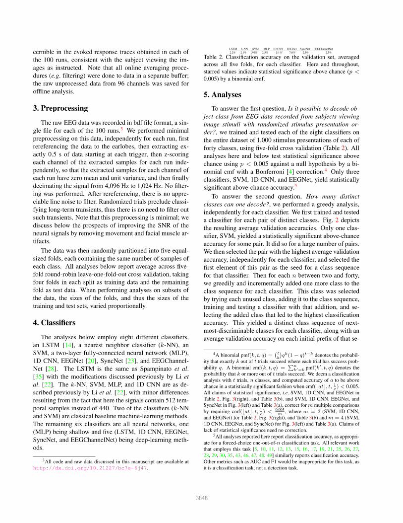
LSTM k-NN SVM MLP 1D CNN EEGNet SyncNet EEGChannelNet
2.2% 2.1% 5.0%∗ 2.5% 5.1%∗ 7.0%∗ 2.5% 2.5%
Table 2. Classification accuracy on the validation set, averaged
across all five folds, for each classifier. Here and throughout,
starred values indicate statistical significance above chance (p <
0.005) by a binomial cmf.
5. Analyses
To answer the first question, Is it possible to decode ob-
ject class from EEG data recorded from subjects viewing
image stimuli with randomized stimulus presentation or-
der?, we trained and tested each of the eight classifiers on
the entire dataset of 1,000 stimulus presentations of each of
forty classes, using five-fold cross validation (Table 2). All
analyses here and below test statistical significance above
chance using p < 0.005 against a null hypothesis by a bi-
nomial cmf with a Bonferroni [4] correction.4 Only three
classifiers, SVM, 1D CNN, and EEGNet, yield statistically
significant above-chance accuracy.5
To answer the second question, How many distinct
classes can one decode?, we performed a greedy analysis,
independently for each classifier. We first trained and tested
a classifier for each pair of distinct classes. Fig. 2 depicts
the resulting average validation accuracies. Only one clas-
sifier, SVM, yielded a statistically significant above-chance
accuracy for some pair. It did so for a large number of pairs.
We then selected the pair with the highest average validation
accuracy, independently for each classifier, and selected the
first element of this pair as the seed for a class sequence
for that classifier. Then for each n between two and forty,
we greedily and incrementally added one more class to the
class sequence for each classifier. This class was selected
by trying each unused class, adding it to the class sequence,
training and testing a classifier with that addition, and se-
lecting the added class that led to the highest classification
accuracy. This yielded a distinct class sequence of next-
most-discriminable classes for each classifier, along with an
average validation accuracy on each initial prefix of that se-
4A binomial pmf(k, t, q) =(
t
k
)
qk(1 − q)t−k denotes the probabil-
ity that exactly k out of t trials succeed where each trial has success prob-
ability q. A binomial cmf(k, t, q) =∑
n
k′=k
pmf(k′, t, q) denotes the
probability that k or more out of t trials succeed. We deem a classification
analysis with t trials, n classes, and computed accuracy of a to be above
chance in a statistically significant fashion when cmf(⌊at⌋, t, 1c) < 0.005.
All claims of statistical significance, i.e. SVM, 1D CNN, and EEGNet in
Table 2, Fig. 3(right), and Table 3(b), and SVM, 1D CNN, EEGNet, and
SyncNet in Fig. 3(left) and Table 3(a), correct for m multiple comparisons
by requiring cmf(⌊at⌋, t, 1c) < 0.005
m, where m = 3 (SVM, 1D CNN,
and EEGNet) for Table 2, Fig. 3(right), and Table 3(b) and m = 4 (SVM,
1D CNN, EEGNet, and SyncNet) for Fig. 3(left) and Table 3(a). Claims of
lack of statistical significance need no correction.5All analyses reported here report classification accuracy, as appropri-
ate for a forced-choice one-out-of-n classification task. All relevant work
that employs this task [5, 10, 11, 12, 13, 15, 16, 17, 19, 21, 25, 26, 27,
28, 29, 30, 35, 43, 46, 47, 48, 49] similarly reports classification accuracy.
Other metrics such as AUC and F1 would be inappropriate for this task, as
it is a classification task, not a detection task.
3848
quence (Fig. 3left and Table 3b).6 With the exception of
a single data point, the MLP classifier achieving marginally
significant above-chance classification accuracy for n = 29,
only four classifiers, SVM, 1D CNN, EEGNet, and Sync-
Net, yielded statistically significant above-chance accuracy
for any number of classes. SVM and 1D CNN yielded sta-
tistically significant above-chance accuracy for all numbers
of classes, EEGNet yielded statistically significant above-
chance accuracy for n ≥ 4, and SyncNet yielded statisti-
cally significant above-chance accuracy for 3 ≤ n ≤ 27.
To answer the third question, How much training data is
needed?, we performed an analysis where classifiers were
trained and tested on progressively larger portions of the
dataset, starting with 10%, incrementing by 10%, until the
full dataset was tested. This was done by taking the first
ten runs and incrementally adding the next ten runs. This
was done only for SVM, 1D CNN, and EEGNet, as only
these had statistically significant above-chance accuracy for
the full set of classes (Fig. 3right and Table 3b). Validation
accuracy generally increases with the availability of more
training data, though growth tapers off demonstrating di-
minishing returns.
The fourth question, Which classification architectures
that are currently standard in the literature allow such de-
coding?, was implicitly answered by the above three anal-
yses. Only SVM, 1D CNN, EEGNet, and SyncNet answer
any of the above three questions in the affirmative. SVM,
1D CNN, and EEGNet answer all of the above three ques-
tions in the affirmative.
To answer the fifth question, Does the inclusion of EEG
data contaminated with artifacts limit the decoding abil-
ity?, we conducted an additional analysis. While we had
a very cooperative subject, the task of watching 40,000 im-
age stimuli can be tedious. It is conceivable that the EEG
recordings suffer from artifacts that reduce classification ac-
curacy. To assess this, we repeated the analyses from Ta-
ble 2 for the three classifiers (SVM, 1D CNN, and EEG-
Net) for which we have observed statistically significant
above-chance classification accuracy, after performing ar-
tifact removal. We computed the swing for each time point
in each trial, i.e. the value of the maximal channel minus the
value of the minimal channel, computed the overall swing
for each trial as the maximal swing over all time points in
that trial, and discarded trials with greater than 600 micro-
Volt swing. A total of 852 out of 40,000 trials (2.13%)
were discarded, maintaining the same splits. This procedure
eliminates trials contaminated by appreciable artifacts from
subject movement and tightening of facial muscles. As a
result, the splits were no longer perfectly counterbalanced.
6The analyses reported in this manuscript require about a year of com-
pute time on a cluster with 144 cores and 54 Titan V GPUs. The results
for EEGChannelNet for n ≥ 26 in Fig. 3(left) and Table 3(a) are being
computed but were not available in time for publication.
Table 3(c) shows the results. While there is improvement
for 1D CNN (5.1% to 5.3%) and EEGNet (7.0% to 7.3%),
the improvement is not statistically significant, suggesting
that artifacts are not the limiting factor in classification ac-
curacy.
To answer the sixth question, Does use of a classifica-
tion method that lacks inherent ability to model temporal
variation in the EEG signal limit decoding ability?, we con-
ducted an additional analysis. The LSTM, 1D CNN, EEG-
Net, SyncNet, and EEGChannelNet classifiers all provide
an inherent ability to compensate for temporal variation in
the signal, both in the onset time of brain processing and its
rate. The k-NN, SVM and MLP classifiers lack such an in-
herent ability. We asked whether such ability materially af-
fects classification accuracy. To this end, we computed 257-
point power spectral density [36] of the raw EEG signal on a
per trial and per channel basis and repeated the analysis with
the k-NN, SVM, and MLP classifiers on this frequency-
domain signal instead of the original time-domain signal
(Table 3d). Such frequency-domain analyses appears not to
improve upon the time-domain analyses. We hypothesize
two reasons for this. First, we recorded the stimulus on-
set time as a trigger in the EEG signal and synchronize our
analyses to this. This eliminates variation in onset time of
the availability of visual information to the brain. Second, it
appears that there is not much variation in brain processing
rate for this task, and that the phase content of the EEG re-
sponse is relatively uninformative for object classification.
Finally, to answer the seventh question, Can one perform
such decoding across subjects?, we performed an additional
analysis. It appears that to achieve even modest statisti-
cally significant above-chance classification accuracy, one
needs enormous amounts of data. It is taxing to collect
this data from a single subject. Perhaps, one could spread
the burden by collecting data from many subjects, perhaps
even across many sites. Doing this, however, would require
cross-subject analyses, i.e. training classifiers on one set of
subjects and testing on a different set of subjects. We con-
ducted an analysis to assess the ability to do so. We reana-
lyzed data from six subjects on a smaller set of fifty shared
stimuli for each of the same forty classes, all collected
with randomized trials [22] using a leave-one-subject-out
six-fold cross-validation paradigm with the three classifiers
(SVM, 1D CNN, and EEGNet) for which we have observed
statistically significant above-chance classification accuracy
(Table 3e). While this analysis (12,000 trials) is not as small
as the analyses in Li et al. [22] (2,000 trials) it is also not as
large as the above analyses (40,000 trials). It corresponds
to the 30% mark in Fig. 3(right) and Table 3(b). Note that
while 1D CNN performs marginally above chance in a sta-
tistically significant fashion, the cross-subject analysis is far
worse (2.9% vs. 4.0% for SVM, 3.6% vs. 5.3% for 1D CNN,
and 2.7% vs. 5.1% for EEGNet). This suggests that per-
3849
LSTM k-NN SVM MLP
1D CNN EEGNet SyncNet EEGChannelNet
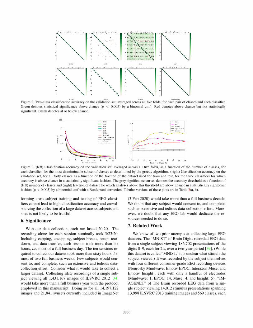
Figure 2. Two-class classification accuracy on the validation set, averaged across all five folds, for each pair of classes and each classifier.
Green denotes statistical significance above chance (p < 0.005) by a binomial cmf. Red denotes above chance but not statistically
significant. Blank denotes at or below chance.
Figure 3. (left) Classification accuracy on the validation set, averaged across all five folds, as a function of the number of classes, for
each classifier, for the most discriminable subset of classes as determined by the greedy algorithm. (right) Classification accuracy on the
validation set, for all forty classes as a function of the fraction of the dataset used for train and test, for the three classifiers for which
accuracy is above chance in a statistically significant fashion. The grey significance curves denotes the accuracy threshold as a function of
(left) number of classes and (right) fraction of dataset for which analyses above this threshold are above chance in a statistically significant
fashion (p < 0.005) by a binomial cmf with a Bonferroni correction. Tabular versions of these plots are in Table 3(a, b).
forming cross-subject training and testing of EEG classi-
fiers cannot lead to high classification accuracy and crowd-
sourcing the collection of a large dataset across subjects and
sites is not likely to be fruitful.
6. Significance
With our data collection, each run lasted 20:20. The
recording alone for each session nominally took 3:23:20.
Including capping, uncapping, subject breaks, setup, tear-
down, and data transfer, each session took more than six
hours, i.e. most of a full business day. The ten sessions re-
quired to collect our dataset took more than sixty hours, i.e.
most of two full business weeks. Few subjects would con-
sent to, and complete, such an extensive and tedious data-
collection effort. Consider what it would take to collect a
larger dataset. Collecting EEG recordings of a single sub-
ject viewing all 1,431,167 images of ILSVRC 2012 [34]
would take more than a full business year with the protocol
employed in this manuscript. Doing so for all 14,197,122
images and 21,841 synsets currently included in ImageNet
(3 Feb 2020) would take more than a full business decade.
We doubt that any subject would consent to, and complete,
such an extensive and tedious data-collection effort. More-
over, we doubt that any EEG lab would dedicate the re-
sources needed to do so.
7. Related Work
We know of two prior attempts at collecting large EEG
datasets. The “MNIST” of Brain Digits recorded EEG data
from a single subject viewing 186,702 presentations of the
digits 0–9, each for 2 s, over a two-year period [39]. (While
this dataset is called “MNIST,” it is unclear what stimuli the
subject viewed.) It was recorded by the subject themselves
with four different consumer-grade EEG recording devices
(Neurosky Mindwave, Emotiv EPOC, Interaxon Muse, and
Emotiv Insight), each with only a handful of electrodes
(Mindwave: 1, EPOC: 14, Muse: 4, and Insight: 5). “IM-
AGENET” of The Brain recorded EEG data from a sin-
gle subject viewing 14,012 stimulus presentations spanning
13,998 ILSVRC 2013 training images and 569 classes, each
3850
accuracy
number of classes LSTM k-NN SVM MLP 1D CNN EEGNet SyncNet EEGChannelNet
2 50.0% 51.3% 70.8%∗ 50.0% 66.4%∗ 50.0% 50.0% 50.0%
3 33.3% 33.8% 56.1%∗ 33.7% 52.5%∗ 35.1% 39.5%∗ 33.3%
4 25.5% 25.1% 44.5%∗ 26.7% 44.1%∗ 30.2%∗ 30.3%∗ 25.3%
5 20.8% 20.7% 37.5%∗ 21.1% 38.4%∗ 24.8%∗ 24.1%∗ 20.3%
6 17.1% 16.9% 32.4%∗ 17.4% 32.8%∗ 21.8%∗ 19.9%∗ 16.7%
7 14.8% 14.4% 28.3%∗ 14.9% 29.8%∗ 19.5%∗ 17.9%∗ 14.9%
8 12.7% 12.6% 25.1%∗ 13.3% 27.1%∗ 17.4%∗ 15.7%∗ 12.9%
9 11.3% 10.9% 22.6%∗ 11.9% 24.7%∗ 18.2%∗ 13.9%∗ 11.7%
10 10.1% 9.7% 20.6%∗ 10.5% 22.0%∗ 17.3%∗ 12.7%∗ 10.3%
11 9.4% 8.7% 18.9%∗ 9.2% 20.9%∗ 17.3%∗ 11.4%∗ 9.6%
12 8.4% 8.1% 17.5%∗ 8.7% 18.4%∗ 16.6%∗ 10.2%∗ 8.8%
13 8.0% 7.4% 16.3%∗ 8.2% 17.2%∗ 15.6%∗ 9.4%∗ 8.0%
14 7.2% 6.9% 15.2%∗ 7.5% 16.2%∗ 15.2%∗ 9.2%∗ 7.2%
15 6.7% 6.4% 14.3%∗ 6.9% 14.8%∗ 15.7%∗ 8.8%∗ 6.9%
16 6.2% 6.0% 13.4%∗ 6.5% 14.0%∗ 15.4%∗ 8.5%∗ 6.6%
17 5.9% 5.7% 12.7%∗ 6.1% 13.6%∗ 14.4%∗ 8.0%∗ 6.0%
18 5.5% 5.3% 12.0%∗ 5.8% 12.5%∗ 13.9%∗ 7.7%∗ 5.7%
19 5.1% 5.0% 11.4%∗ 5.4% 11.9%∗ 13.4%∗ 6.7%∗ 5.5%
20 4.8% 4.7% 10.8%∗ 5.3% 11.0%∗ 12.7%∗ 6.0%∗ 5.1%
21 4.7% 4.5% 10.3%∗ 4.9% 10.9%∗ 12.0%∗ 5.7%∗ 4.9%
22 4.4% 4.2% 9.8%∗ 4.8% 10.0%∗ 11.7%∗ 5.4%∗ 4.6%
23 4.2% 4.1% 9.4%∗ 4.5% 9.4%∗ 11.2%∗ 4.9%∗ 4.4%
24 4.0% 3.9% 9.0%∗ 4.4% 9.4%∗ 10.9%∗ 4.9%∗ 4.3%
25 3.8% 3.8% 8.6%∗ 4.0% 9.1%∗ 10.7%∗ 4.4%∗ 4.0%
26 3.7% 3.6% 8.3%∗ 3.9% 8.6%∗ 10.5%∗ 4.2%∗
27 3.5% 3.5% 8.0%∗ 4.0% 8.1%∗ 10.1%∗ 4.0%∗
28 3.5% 3.4% 7.7%∗ 3.7% 8.1%∗ 9.9%∗ 3.7%
29 3.3% 3.3% 7.4%∗ 3.8%∗ 7.5%∗ 9.7%∗ 3.6%
30 3.4% 3.2% 7.2%∗ 3.3% 7.3%∗ 9.9%∗ 3.4%
31 3.1% 3.1% 6.9%∗ 3.4% 7.1%∗ 9.3%∗ 3.3%
32 3.0% 3.0% 6.7%∗ 3.2% 7.0%∗ 9.1%∗ 3.2%
33 3.0% 2.8% 6.5%∗ 3.1% 6.7%∗ 8.8%∗ 3.0%
34 2.8% 2.7% 6.3%∗ 2.9% 6.4%∗ 8.6%∗ 3.0%
35 2.8% 2.6% 6.1%∗ 2.8% 6.4%∗ 8.6%∗ 2.9%
36 2.6% 2.5% 5.9%∗ 2.7% 6.2%∗ 8.6%∗ 2.7%
37 2.6% 2.4% 5.7%∗ 2.8% 6.1%∗ 8.0%∗ 2.7%
38 2.5% 2.3% 5.5%∗ 2.6% 5.9%∗ 7.6%∗ 2.6%
39 2.4% 2.2% 5.3%∗ 2.5% 5.7%∗ 7.4%∗ 2.6%
40 2.3% 2.1% 5.2%∗ 2.4% 5.4%∗ 7.2%∗ 2.5%
(a)
accuracy
fraction of dataset SVM 1D CNN EEGNet
10% 2.9% 3.4%∗ 3.8%∗
20% 3.7%∗ 4.6%∗ 5.1%∗
30% 4.0%∗ 5.3%∗ 5.1%∗
40% 4.6%∗ 5.7%∗ 6.9%∗
50% 4.2%∗ 5.7%∗ 7.4%∗
60% 4.7%∗ 5.9%∗ 7.5%∗
70% 4.8%∗ 5.4%∗ 7.0%∗
80% 4.8%∗ 5.4%∗ 7.3%∗
90% 4.8%∗ 5.3%∗ 7.4%∗
100% 5.0%∗ 5.1%∗ 7.0%∗
(b)
SVM 1D CNN EEGNet
5.0%∗ 5.3%∗ 7.3%∗
(c)
k-NN SVM MLP
2.1% 3.3%∗ 1.6%
(d)
SVM 1D CNN EEGNet
2.9% 3.6%∗ 2.7%
(e)
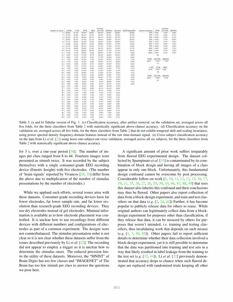
Table 3. (a and b) Tabular version of Fig. 3. (c) Classification accuracy, after artifact removal, on the validation set, averaged across all
five folds, for the three classifiers from Table 2 with statistically significant above-chance accuracy. (d) Classification accuracy on the
validation set, averaged across all five folds, for the three classifiers from Table 2 that do not exhibit temporal shift and scaling invariance,
using power spectral density frequency-domain features instead of the raw time-domain signal. (e) Cross-subject classification accuracy
on the data from Li et al. [22] using leave-one-subject-out cross validation, averaged across all six subjects, for the three classifiers from
Table 2 with statistically significant above-chance accuracy.
for 3 s, over a one-year period [38]. The number of im-
ages per class ranged from 8 to 44. Fourteen images were
presented as stimuli twice. It was recorded by the subject
themselves with a single consumer-grade EEG recording
device (Emotiv Insight) with five electrodes. (The number
of ‘brain signals’ reported by Vivancos [38, 39] differ from
the above due to multiplication of the number of stimulus
presentations by the number of electrodes.)
While we applaud such efforts, several issues arise with
these datasets. Consumer-grade recording devices have far
fewer electrodes, far lower sample rate, and far lower res-
olution than research-grade EEG recording devices. They
use dry electrodes instead of gel electrodes. Minimal infor-
mation is available as to how electrode placement was con-
trolled. It is unclear how to use recordings from different
devices with different numbers and configurations of elec-
trodes as part of a common experiment. The designs were
not counterbalanced. The stimulus presentation order is not
clear so it is not clear whether these datasets suffer from the
issues described previously by Li et al. [22]. The recording
did not appear to employ a trigger so it is unclear how to
determine the stimulus onset. The reduced precision lim-
its the utility of these datasets. Moreover, the “MNIST” of
Brain Digits has too few classes and “IMAGENET” of The
Brain has too few stimuli per class to answer the questions
we pose here.
A significant amount of prior work suffers irreparably
from flawed EEG experimental design. The dataset col-
lected by Spampinato et al. [35] is contaminated by its com-
bination of block design and having all images of a class
appear in only one block. Unfortunately, this fundamental
design confound cannot be overcome by post processing.
Considerable follow-on work [5, 10, 11, 12, 13, 15, 16, 17,
19, 21, 25, 26, 27, 28, 29, 30, 43, 46, 47, 48, 49] that uses
this dataset also inherits this confound and their conclusions
may thus be flawed. Other papers also report collection of
data from a block-design experiment, and train and test clas-
sifiers on that data (e.g. [2, 24, 42]) Further, it has become
popular to publicly release data for others to reuse. While
original authors can legitimately collect data from a block-
design experiment for purposes other than classification, if
they release that data, it can be misused by others for pur-
poses that weren’t intended, i.e. training and testing clas-
sifiers, thus invalidating work that depends on such misuse
(e.g. [1, 3, 40, 45]). Other papers fail to report sufficient
details to determine whether their data collection involved a
block-design experiment, yet it is still possible to determine
that the data was partitioned into training and test sets in a
way that likely resulted in label leakage from the training to
the test set (e.g. [32, 44]). Li et al. [22] previously demon-
strated that accuracy drops to chance when such flawed de-
signs are replaced with randomized trials keeping all other
3851
aspects of the experimental design unchanged, including the
dataset size. Here, we demonstrate that accuracy increases
to only marginally above significance even when the dataset
size is increased to the bounds of feasibility.
8. Conclusion
In this manuscript we demonstrate five novel contribu-
tions.
1. We show that it does not seem possible to decode ob-
ject class from EEG data recorded from subjects view-
ing image stimuli with randomized stimulus presen-
tation order when the dataset contains between two
and forty classes with classification accuracy that is
above chance in a statistically significant fashion us-
ing an LSTM (the classifier employed by Spampinato
et al. [35]), a k-NN classifier, an MLP classifier, or
EEGChannelNet, even if one has a training set that
is 20× larger than previous work. It appears that
the LSTM, k-NN, MLP, and EEGChannelNet classi-
fiers are ill-suited to classifying object class from EEG
data recorded from subjects viewing image stimuli no
matter how many classes are classified and no mat-
ter how much training data is available. This refutes
a large amount of prior work and shows that the task
attempted by that work is simply infeasible.
2. We show that it is possible to decode object class from
EEG data recorded from subjects viewing image stim-
uli with randomized stimulus presentation order when
the dataset contains between two and forty classes with
classification accuracy that is marginally above chance
in a statistically significant fashion using either SVM,
1D CNN, EEGNet, or SyncNet. However, it is not pos-
sible to obtain accuracy above chance in a statistically
significant fashion with a dataset of the size employed
by previous work (fifty samples per class). For forty
classes, accuracy is marginally below statistical signif-
icance for SVM and marginally above statistical sig-
nificance for 1D CNN and EEGNet with 100 samples
per class (2× previous work), increases to about 5%
for the SVM, about 6% for 1D CNN, and about 8% for
EEGNet with about 600 samples per class (12× pre-
vious work), and then tapers off. It appears that no
amount of additional training data will allow substan-
tially better classification accuracy for forty classes us-
ing the classifiers that we tried.
3. Our classification accuracies are state-of-the-art for de-
coding object class from EEG data recorded from sub-
jects viewing image stimuli with randomized stimu-
lus presentation and large numbers of classes. To
our knowledge, these are also the first results yielding
statistically significant above-chance accuracy with a
large number of classes. Previous reports of higher ac-
curacy, to the best of our knowledge, appear to use data
that are contaminated by the confounds we describe.
4. We show that gathering the amounts of training data to
achieve this level of accuracy are at the bounds of fea-
sibility. Gathering the requisite data to train classifiers
for a larger number of classes, such as all of ILSVRC
2012, let alone all of ImageNet, would require Her-
culean effort.
5. We collected by far the largest known dataset of EEG
recordings from a single subject viewing image stimuli
with professional-grade equipment and procedures us-
ing proper randomized trials. It has 20× as many stim-
uli per class as the dataset of Li et al. [22], 4× as many
classes as the dataset of Vivancos [39] (which is not
known to have randomized trials), and 23× to 125×
as many stimuli per class as the dataset of Vivancos
[38] (which is also not known to have randomized tri-
als). Our released dataset will facilitate experimenta-
tion with new classification and analysis methods that
will hopefully lead to improved accuracy in the future.
Despite recent claims to the contrary, presented to the
computer-vision community with great fanfare, the problem
of classifying visually perceived objects from EEG record-
ings with high accuracy for large numbers of classes is im-
mensely difficult and currently beyond the state of the art. It
appears to be infeasible absent fundamentally groundbreak-
ing improvements to EEG technology or classification ap-
proaches. A common euphoria in the community is that
large datasets have allowed deep-learning methods to solve
practically everything. It appears, however, to have reached
its limit with object classification from EEG recordings.
Neither heroic amounts of data, at the bounds of feasibility,
traditional machine-learning methods like nearest-neighbor
classifiers (k-NN) or support vector machines (SVM), the
standard neural-network architectures of fully connected
networks (MLP), convolutional neural networks (CNN), or
recurrent neural networks (LSTM), nor even newer deep-
learning methods like EEGNet, SyncNet, or EEGChannel-
Net appear suited to the task. We present our data and this
task to the community as a challenge problem. A deeper
understanding of human visual perception that moves be-
yond large datasets and deep learning is perhaps necessary
to solve this problem.
Acknowledgments
This work was supported, in part, by NSF Grants1522954-IIS and 1734938-IIS, IARPA DOI/IBC contractD17PC00341, NIH Grant R01DC015989, and SiemensCorporation. Any findings, views, conclusions, and recom-mendations in this material are those of the authors and donot necessarily reflect the views, policies, or endorsements,expressed or implied, of the sponsors. The U.S. Govern-ment is authorized to reproduce and distribute reprints forGovernment purposes, notwithstanding any copyright nota-tion herein.
3852
References
[1] Salma Alhagry, Aly Aly Fahmy, and Reda A El-Khoribi.
Emotion recognition based on EEG using LSTM recurrent
neural network. International Journal of Advanced Com-
puter Science and Applications, 8(10):8–11, 2017. 7
[2] Jinwon An and Sungzoon Cho. Hand motion identification
of grasp-and-lift task from electroencephalography record-
ings using recurrent neural networks. In International Con-
ference on Big Data and Smart Computing, pages 427–429,
2016. 7
[3] Ahmed Ben Said, Amr Mohamed, Tarek Elfouly, Khaled
Harras, and Z Jane Wang. Multimodal deep learning ap-
proach for joint EEG-EMG data compression and classifica-
tion. In Wireless Communications and Networking Confer-
ence, 2017. 7
[4] Carlo E. Bonferroni. Teoria statistica delle classi e cal-
colo delle probabilita. Pubblicazioni del R Istituto Superiore
di Scienze Economiche e Commerciali di Firenze, 8:3–62,
1936. 4
[5] Alberto Bozal. Personalized image classification from
EEG signals using deep learning. B.S. thesis, Universitat
Politecnica de Catalunya, 2017. 1, 2, 4, 7
[6] Corinna Cortes and Vladimir Vapnik. Support-vector net-
works. Machine Learning, 20(3):273–297, 1995. 2
[7] Alexander Craik, Yongtian He, and Jose L Contreras-Vidal.
Deep learning for electroencephalogram (EEG) classifica-
tion tasks: a review. Journal of Neural Engineering, 16(3),
2019. 1
[8] Nicolae Cudlencu, Nirvana Popescu, and Marius Leordeanu.
Reading into the mind’s eye: Boosting automatic visual
recognition with EEG signals. Neurocomputing, available
online 23 December 2019, 2019. 1, 2
[9] Jia Deng, Wei Dong, Richard Socher, Li-Jia Li, Kai Li,
and Li Fei-Fei. ImageNet: A large-scale hierarchical im-
age database. In Computer Vision and Pattern Recognition,
pages 248–255, 2009. 1
[10] Changde Du, Changying Du, and Huiguang He. Doubly
semi-supervised multimodal adversarial learning for classifi-
cation, generation and retrieval. In International Conference
on Multimedia, pages 13–18, 2019. 1, 2, 4, 7
[11] Changying Du, Changde Du, Xingyu Xie, Chen Zhang, and
Hao Wang. Multi-view adversarially learned inference for
cross-domain joint distribution matching. In International
Conference on Knowledge Discovery & Data Mining, pages
1348–1357, 2018. 1, 2, 4, 7
[12] Ahmed Fares, Shenghua Zhong, and Jianmin Jiang. Region
level bi-directional deep learning framework for EEG-based
image classification. In International Conference on Bioin-
formatics and Biomedicine, pages 368–373, 2018. 1, 2, 4,
7
[13] Ahmed Fares, Sheng-hua Zhong, and Jianmin Jiang. Brain-
media: A dual conditioned and lateralization supported GAN
(DCLS-GAN) towards visualization of image-evoked brain
activities. In International Conference on Multimedia, pages
1764–1772, 2020. 1, 2, 4, 7
[14] Sepp Hochreiter and Jurgen Schmidhuber. Long short-term
memory. Neural Computation, 9(8):1735–1780, 1997. 4
[15] Sunhee Hwang, Kibeom Hong, Guiyoung Son, and Hyeran
Byun. EZSL-GAN: EEG-based zero-shot learning approach
using a generative adversarial network. In International Win-
ter Conference on Brain-Computer Interface, 2019. 1, 2, 4,
7
[16] Jianmin Jiang, Ahmed Fares, and Sheng-Hua Zhong. A
context-supported deep learning framework for multimodal
brain imaging classification. Transactions on Human-
Machine Systems, 2019. 1, 2, 4, 7
[17] Zhicheng Jiao, Haoxuan You, Fan Yang, Xin Li, Han Zhang,
and Dinggang Shen. Decoding EEG by visual-guided deep
neural networks. In International Joint Conference on Arti-
ficial Intelligence, 2019. 1, 2, 4, 7
[18] Ashish Kapoor, Pradeep Shenoy, and Desney Tan. Combin-
ing brain computer interfaces with vision for object catego-
rization. In Computer Vision and Pattern Recognition, 2008.
2
[19] Isaak Kavasidis, Simone Palazzo, Concetto Spampinato,
Daniela Giordano, and Mubarak Shah. Brain2Image: Con-
verting brain signals into images. In International Confer-
ence on Multimedia, pages 1809–1817, 2017. 1, 2, 4, 7
[20] V. J. Lawhern, A. J. Solon, N. R. Waytowich, S. M. Gordon,
C. P. Hung, and B. J. Lance. EEGNet: a compact convolu-
tional neural network for EEG-based brain-computer inter-
faces. Journal of Neural Engineering, 15(5):056013, 2018.
2, 4
[21] Dan Li, Changde Du, and Huiguang He. Semi-supervised
cross-modal image generation with generative adversarial
networks. Pattern Recognition, 100, 2020. 1, 2, 4, 7
[22] Ren Li, Jared S. Johansen, Hamad Ahmed, Thomas V.
Ilyevsky, Ronnie B. Wilbur, Hari M. Bharadwaj, and Jef-
frey Mark Siskind. The perils and pitfalls of block design
for EEG classification experiments. Transactions on Pattern
Analysis and Machine Intelligence, 43(1):316–333, 2021. 1,
2, 4, 5, 7, 8
[23] Y. Li, M. Murias, S. Major, G. Dawson, K. Dzirasa, L. Carin,
and D. E. Carlson. Targeting EEG/LFP synchrony with neu-
ral nets. In Advances in Neural Information Processing Sys-
tems, pages 4620–4630, 2017. 2, 4
[24] A. K. Mohamed, T. Marwala, and L. R. John. Single-trial
EEG discrimination between wrist and finger movement im-
agery and execution in a sensorimotor BCI. In International
Conference of the Engineering in Medicine and Biology So-
ciety, 2011. 7
[25] Pranay Mukherjee, Abhirup Das, Ayan Kumar Bhunia, and
Partha Pratim Roy. Cogni-Net: Cognitive feature learning
through deep visual perception. In International Conference
on Image Processing, pages 4539–4543, 2019. 1, 2, 4, 7
[26] Simone Palazzo, Isaak Kavasidis, Dimitris Kastaniotis, and
Stavros Dimitriadis. Recent advances at the brain-driven
computer vision workshop. In European Conference on
Computer Vision, 2018. 1, 2, 4, 7
[27] Simone Palazzo, Francesco Rundo, Sebastiano Battiato,
Daniela Giordano, and Concetto Spampinato. Visual
saliency detection guided by neural signals. In Interna-
tional Conference on Automatic Face and Gesture Recog-
nition, pages 434–440, 2020. 1, 2, 4, 7
3853
[28] Simone Palazzo, Concetto Spampinato, Isaak Kavasidis,
Daniela Giordano, Joseph Schmidt, and Mubarak Shah. De-
coding brain representations by multimodal learning of neu-
ral activity and visual features. Transactions on Pattern
Analysis and Machine Intelligence, 2020. 1, 2, 4, 7
[29] Simone Palazzo, Concetto Spampinato, Isaak Kavasidis,
Daniela Giordano, and Mubarak Shah. Generative adversar-
ial networks conditioned by brain signals. In International
Conference on Computer Vision, pages 3410–3418, 2017. 1,
2, 4, 7
[30] Simone Palazzo, Concetto Spampinato, Isaak Kavasidis,
Daniela Giordano, and Mubarak Shah. Decoding brain rep-
resentations by multimodal learning of neural activity and
visual features. arXiv, 1810.10974, 2018. 1, 2, 4, 7
[31] Viral Parekh, Ramanathan Subramanian, Dipanjan Roy, and
CV Jawahar. An EEG-based image annotation system. In
National Conference on Computer Vision, Pattern Recogni-
tion, Image Processing, and Graphics, pages 303–313, 2017.
2
[32] Tanya Piplani, Nick Merill, and John Chuang. Faking it,
making it: Fooling and improving brain-based authentica-
tion with generative adversarial networks. In International
Conference on Biometrics Theory, Applications and Systems,
2018. 7
[33] Yannick Roy, Hubert Banville, Isabela Albuquerque,
Alexandre Gramfort, Tiago H Falk, and Jocelyn Faubert.
Deep learning-based electroencephalography analysis: a
systematic review. Journal of Neural Engineering, 16, 2019.
1
[34] Olga Russakovsky, Jia Deng, Hao Su, Jonathan Krause, San-
jeev Satheesh, Sean Ma, Zhiheng Huang, Andrej Karpathy,
Aditya Khosla, Michael Bernstein, Alexander C. Berg, and
Li Fei-Fei. ImageNet large scale visual recognition chal-
lenge. International journal of computer vision, 115(3):211–
252, 2015. 6
[35] Concetto Spampinato, Simone Palazzo, Isaak Kavasidis,
Daniela Giordano, Nasim Souly, and Mubarak Shah. Deep
learning human mind for automated visual classification.
In Computer Vision and Pattern Recognition, pages 6809–
6817, 2017. 1, 2, 3, 4, 7, 8
[36] David J Thomson. Spectrum estimation and harmonic anal-
ysis. Proceedings of the IEEE, 70(9):1055–1096, 1982. 5
[37] A. C. Metting Van Rijn, A. Peper, and C. A. Grimber-
gen. High-quality recording of bioelectric events. Medical
and Biological Engineering and Computing, 28(5):389–397,
1990. 3
[38] David Vivancos. “IMAGENET” of the brain, 2018. 7, 8
[39] David Vivancos. The “MNIST” of brain digits, 2019. 6, 7, 8
[40] Fang Wang, Sheng Hua Zhong, Jianfeng Peng, Jianmin
Jiang, and Yan Liu. Data augmentation for EEG-based emo-
tion recognition with deep convolutional neural networks.
Lecture Notes in Computer Science, 10705:82–93, 2018. 7
[41] Jun Wang, Eric Pohlmeyer, Barbara Hanna, Yu-Gang Jiang,
Paul Sajda, and Shih-Fu Chang. Brain state decoding for
rapid image retrieval. In International Conference on Multi-
media, pages 945–954, 2009. 2
[42] Pan Wang, Danlin Peng, Ling Li, Liuqing Chen, Chao Wu,
Xiaoyi Wang, Peter Childs, and Yike Guo. Human-in-the-
loop design with machine learning. In International Confer-
ence on Engineering Design, pages 2577–2586, 2019. 7
[43] Wenxiang Zhang and Qingshan Liu. Using the center loss
function to improve deep learning performance for EEG sig-
nal classification. In International Conference on Advanced
Computational Intelligence, pages 578–582, 2018. 1, 2, 4, 7
[44] X. Zhang, L. Yao, Q. Z. Sheng, S. S. Kanhere, T. Gu, and
D. Zhang. Converting your thoughts to texts: Enabling brain
typing via deep feature learning of EEG signals. In Interna-
tional Conference on Pervasive Computing and Communica-
tions, 2018. 7
[45] Xiang Zhang, Lina Yao, Dalin Zhang, Xianzhi Wang,
Quan Z. Sheng, and Tao Gu. Multi-person brain activity
recognition via comprehensive EEG signal analysis. In In-
ternational Conference on Mobile and Ubiquitous Systems:
Computing, Networking and Services, 2017. 7
[46] Xiao Zheng and Wanzhong Chen. An attention-based bi-
LSTM method for visual object classification via EEG.
Biomedical Signal Processing and Control, 63, 2021. 1, 2,
4, 7
[47] Xiao Zheng, Wanzhong Chen, Mingyang Li, Tao Zhang,
Yang You, and Yun Jiang. Decoding human brain activity
with deep learning. Biomedical Signal Processing and Con-
trol, 56, 2020. 1, 2, 4, 7
[48] Xiao Zheng, Wanzhong Chen, Yang You, Yun Jiang,
Mingyang Li, and Tao Zhang. Ensemble deep learning for
automated visual classification using EEG signals. Pattern
Recognition, 102, 2020. 1, 2, 4, 7
[49] Saisai Zhong, Yadong Liu, Zongtan Zhou, and Dewen Hu.
ELSTM-based visual decoding from singal [sic]-trial EEG
recording. In International Conference on Software Engi-
neering and Service Science, pages 1139–1142, 2018. 1, 2,
4, 7
3854