object localization, segmentation, classification, …...object localization, segmentation,...
TRANSCRIPT

Object Localization, Segmentation,Classification, and Pose Estimation in 3D
Images using Deep Learning
by
Allan Zelener
A dissertation proposal submitted to the Graduate Faculty in Computer Science inpartial fulfillment of the requirements for the degree of Doctor of Philosophy, TheCity University of New York.
2016

ii
c©2016
Allan Zelener
All Rights Reserved
iii
ABSTRACT
Object Localization, Segmentation,Classification, and Pose Estimation in 3D
Images Using Deep Learning
by
Allan Zelener
Advisor: Ioannis Stamos
We address the problem of identifying objects of interest in 3D images as a setof related tasks involving localization of objects within a scene, segmentation ofobserved object instances from other scene elements, classifying detected objectsinto semantic categories, and estimating the 3D pose of detected objects withinthe scene. The increasing availability of 3D sensors motivates us to leverage largeamounts of 3D data to train machine learning models to address these tasks in 3Dimages. Recent advances in deep learning lead us to propose a model capable ofbeing optimized for all of these tasks jointly in order to reduce potential errorspropagated when solving these tasks independently.

Contents
1 Introduction 1
2 Completed Work 6
2.1 Part-Based Object Classification . . . . . . . . . . . . . . . . . . 7
2.2 CNN-Based Object Segmentation . . . . . . . . . . . . . . . . . 21
2.3 Related Work . . . . . . . . . . . . . . . . . . . . . . . . . . . . 37
3 Proposed Work 41
3.1 Timeline for Completion . . . . . . . . . . . . . . . . . . . . . . 49
iv
Chapter 1
Introduction
Our world is a three-dimensional environment and in order for our automated sys-
tems to effectively interact with this environment they need to model and reason
about the objects of interest that inhabit the world which are necessary to solve a
given task. For example these could be vehicles and pedestrians that a self-driving
car must avoid colliding with or products stored in a warehouse that a robot must
collect for shipping. These systems would employ visual sensors that typically
acquire 2D images of the 3D world. It is from these images that we must recover
the inherent 3D properties of objects in the world to enable higher-level tasks.
Identifying objects of interest in images involves solving a set of related tasks.
Given an image of a scene it is first necessary to find the general location of each
object within the image, for example by estimating a bounding box for each pos-
sible object. Next this localization may be refined by segmenting the image pixels
corresponding to the localized objects from other parts of the scene. Finally given
1
CHAPTER 1. INTRODUCTION 2
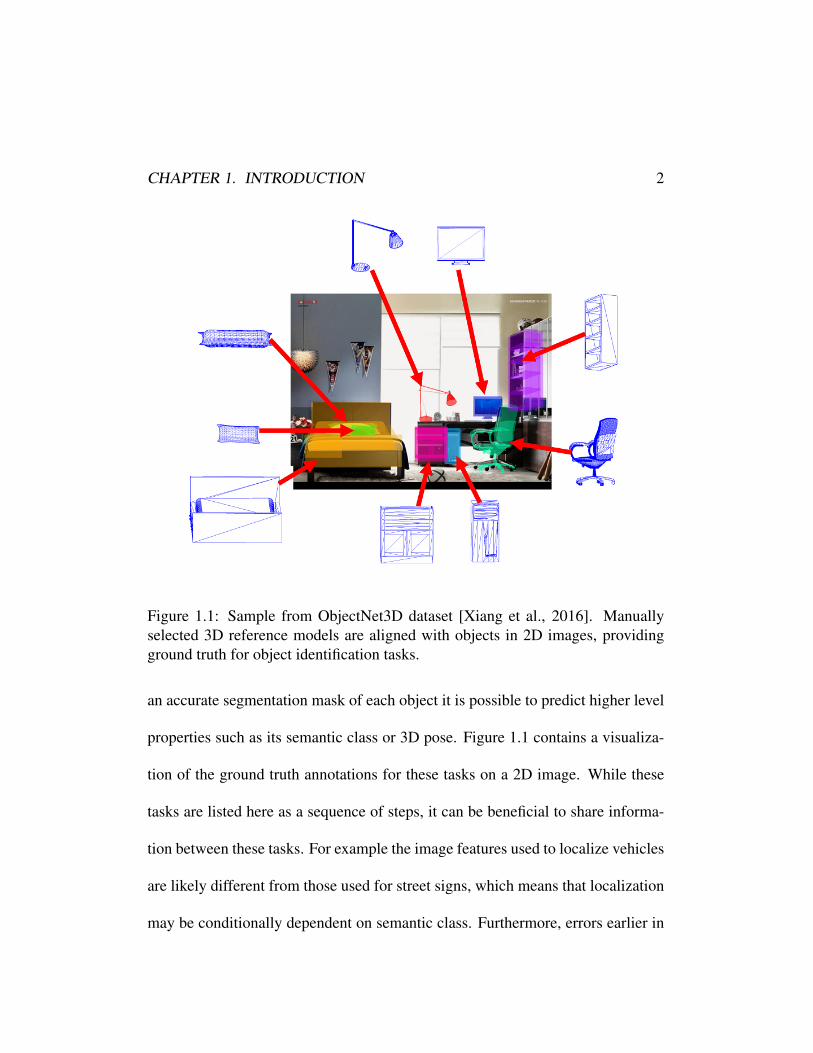
Figure 1.1: Sample from ObjectNet3D dataset [Xiang et al., 2016]. Manuallyselected 3D reference models are aligned with objects in 2D images, providingground truth for object identification tasks.
an accurate segmentation mask of each object it is possible to predict higher level
properties such as its semantic class or 3D pose. Figure 1.1 contains a visualiza-
tion of the ground truth annotations for these tasks on a 2D image. While these
tasks are listed here as a sequence of steps, it can be beneficial to share informa-
tion between these tasks. For example the image features used to localize vehicles
are likely different from those used for street signs, which means that localization
may be conditionally dependent on semantic class. Furthermore, errors earlier in
CHAPTER 1. INTRODUCTION 3
the process may be propagated to later tasks. It is not possible to correctly classify
an object if it was never detected as an object of interest within the scene.
Accurately estimating an object’s 3D shape and pose from a single 2D image
using a traditional camera is a difficult task, in fact if no simplifying assumptions
about visual cues are used then it is an underdetermined problem with infinitely
many solutions. Fortunately in recent years there has been a steady increase in the
availability of 3D sensors capable of accurate pointwise depth measurements such
as LIDAR scanners for outdoor and aerial sensing or RGB-D cameras for short-
range indoor use, including consumer level sensors like the Microsoft Kinect or
Google Tango. This 3D data introduces its own set of challenges. The density
of 3D point measurements may vary throughout a scene depending on the dis-
tance of scanned surfaces from the sensor. It is also possible to have missing data
due to incompatibility between a surface’s reflectance properties and the scanning
technology, for example glass windows often refract a LIDAR scanner’s laser and
glossy paint on cars can reflect it. There will also still be unobserved parts of
any given object due to self-occlusion or other occluding scene elements so these
3D scans would only partially match reference models. However despite all these
issues there are inherent advantages to using these sensors. The 3D depth mea-
surements directly connect the 2D projections of an environment perceived by a
sensor with the environment’s 3D shape, constraining the problems found in color

CHAPTER 1. INTRODUCTION 4
images such as scale ambiguity or camouflage-like textures.
Figure 1.2: Multi-task cascade network [Dai et al., 2016b]. Object localization,segmentation, and classification are solved in sequence using jointly learned fea-tures in a deep neural network.
By leveraging the large amounts of 3D data that can be collected with 3D
sensors we are able to train machine learning models that solve the object iden-
tification tasks. Deep learning models using convolutional neural networks have
become state-of-the-art on a variety of 2D vision tasks including image classifi-
cation [Krizhevsky et al., 2012, He et al., 2016] and segmentation [Long et al.,
2015]. These deep artificial neural networks provide a general framework for
optimization-based feature extraction on the target task that outperforms previ-
ous manually designed feature extractors. The modeling flexibility provided by
deep learning also allows tasks to be solved jointly and the entire model trained
end-to-end, for example [Dai et al., 2016b] uses a multi-task cascade for object

CHAPTER 1. INTRODUCTION 5
localization, segmentation, and classification as shown in Figure 1.2.
Here we propose to extend deep learning methods to the domain of 3D images
and develop a model that incorporates the tasks of object localization, segmenta-
tion, classification, and pose estimation with a design based on recently proposed
techniques for these tasks. Additionally, we would like to experiment with domain
adaptation from synthetic data given the limited availability of large-scale labeled
3D datasets and address the challenges posed by missing data in 3D images. In
Chapter 2 we describe in detail our completed work on these problems and give a
brief review of related work in 3D computer vision that will motivate and inform
the design of our proposed model. Chapter 3 describes the details of the proposed
work and our proposed experiments for evaluating the model. The timeline for
completing the proposed work is described in Chapter 3.1.
Chapter 2
Completed Work
Identifying objects in images is a topic that has been extensively covered in the
computer vision literature from a variety of perspectives. Our survey [Zelener,
2014] has examined prior work on object classification and segmentation in 3D
range scans which could broadly be categorized into either 3D point clustering
methods for outdoor scenes or 2D image based methods for indoor RGB-D scenes.
Our two prior works towards the proposed dissertation have together investigated
both of these approaches for object classification in urban LIDAR scans. In one
approach [Zelener et al., 2014] we utilize planar point clustering to estimate ob-
ject parts with a structured prediction model to jointly classify the object parts
and overall object category. We have also developed a 2D convolutional neural
network approach on the scanning acquisition grid of urban LIDAR to perform
semantic segmentation over missing data points [Zelener and Stamos, 2016]. In
the following sections we will describe our prior work in more detail and then
6

CHAPTER 2. COMPLETED WORK 7
review some recent related work that has been released since our survey that will
inform our proposed work.
2.1 Part-Based Object Classification
Initial work on object classification for localized object candidates in 3D scenes
[Golovinskiy et al., 2009] has utilized aggregations of simple local features like
spin images [Johnson and Hebert, 1999] to generate global feature descriptors for
candidate objects. We observe however that this approach does not capture the
fine-grained variations in shape which are needed to discriminate between sim-
ilar semantic categories. For example different classes of vehicles like sedans
and SUVs have similar global shapes and it is necessary to utilize specific lo-
cal properties, such as curvature of the sides or the angle at which the car trunk
is joined to other parts. Furthermore, in 3D range scans the object is often par-
tially observed and so an aggregation of local features may be more indicative of
the sensor’s relative viewpoint rather than the object category. To address these
challenges we adopt a parts-based approach using planar clustering inspired by
earlier work that used a simple three-part front/middle/back segmentation on syn-
thetic models [Huber et al., 2004]. By associating local features to object parts
and computing additional features between adjacent parts we are able to build a
structured global representation for the entire object that captures its observed 3D
CHAPTER 2. COMPLETED WORK 8
shape using a piecewise planar approximation.
The model consists of a four stage pipeline composed of local feature extrac-
tion, RANSAC-based part segmentation, part-level feature extraction, and struc-
tured part modeling. We evaluate our model on a collection of vehicle point clouds
that have been manually extracted from the Wright State Ottawa dataset which
consists of unstructured point clouds that have been registered together from both
ground and aerial LIDAR scans of Ottawa. We show that our structured prediction
model achieves superior classification accuracy for object parts and can improve
overall object classification.
Local Feature Extraction
We define local features as statistics computed with respect to a reference point us-
ing neighboring points within a fixed radius as support. For 3D feature descriptors
these are typically histograms of neighboring point positions or surface normal
orientations parameterized within the support space. For this work we selected
the spin image [Johnson and Hebert, 1999] feature descriptor which utilizes an
estimated surface normal at the reference point to parameterize the support space
resulting in a rotationally invariant descriptor.
In order to ensure only those reference points with well-populated supports
are used we use a statistical outlier filter to remove points whose nearest neigh-
CHAPTER 2. COMPLETED WORK 9
bors have an average distance beyond one standard deviation of the mean average
distance for all points within a given object. For the remaining points we esti-
mate surface normals using PCA and orient them away from the centroid of the
object’s footprint on the ground. Spin images are computed on a dense subsam-
pling of these points using a fine-grained voxel grid. In order to adjust for variable
density in our scans we weight the contribution of each point to a spin image by
its inverse density, which is the inverse of the number of neighbors within a fixed
radius.
We use a large support radius for computing spin images so that the local fea-
tures can capture global object shape and the relative position of the reference
point. This parameterization makes the features more amenable to the task of
object classification and for use in a visual bag-of-words descriptor rather than
finding locally unique points when doing keypoint detection for exact matching.
This descriptor will be used as our baseline global object descriptor and as a com-
ponent of the part-level object descriptor.
Part Segmentation
For part segmentation we assume that our objects of interest have roughly piece-
wise planar exteriors which is a reasonable assumption for man-made objects at
the level of detail found in range scans. Our segmentation method is unsupervised
CHAPTER 2. COMPLETED WORK 10
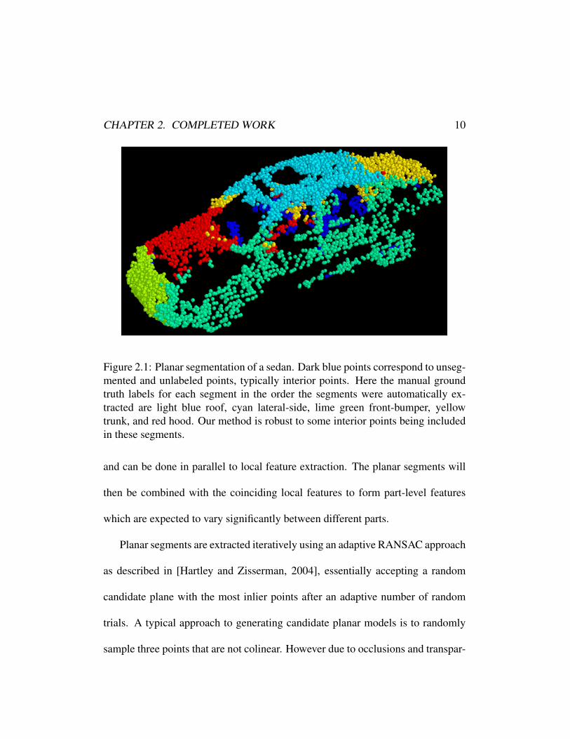
Figure 2.1: Planar segmentation of a sedan. Dark blue points correspond to unseg-mented and unlabeled points, typically interior points. Here the manual groundtruth labels for each segment in the order the segments were automatically ex-tracted are light blue roof, cyan lateral-side, lime green front-bumper, yellowtrunk, and red hood. Our method is robust to some interior points being includedin these segments.
and can be done in parallel to local feature extraction. The planar segments will
then be combined with the coinciding local features to form part-level features
which are expected to vary significantly between different parts.
Planar segments are extracted iteratively using an adaptive RANSAC approach
as described in [Hartley and Zisserman, 2004], essentially accepting a random
candidate plane with the most inlier points after an adaptive number of random
trials. A typical approach to generating candidate planar models is to randomly
sample three points that are not colinear. However due to occlusions and transpar-

CHAPTER 2. COMPLETED WORK 11
ent surfaces that expose an object’s interior, such as windows on a car, it is possible
to fit planes that intersect through the object interior and don’t correspond to se-
mantically identifiable surface components. We avoid these undesirable candidate
planes by estimating the convex hull of the object point cloud using the QHull al-
gorithm [Barber et al., 1996] and sampling candidate planes from the faces of the
convex hull. Due to noise in the sensor measurements, outliers can bias the planes
given by the convex hull so we robustly reestimate each selected plane through
expectation-maximization using PCA. We assume the observed surface of our ob-
ject can be explained with a small number of large planar components and so limit
the total number of planar segments to five or stop when at least 90% of points are
segmented. An example of the resulting segmentation can be seen in Figure 2.1.
Part-Level Feature Extraction
The densely sampled local descriptors are combined with their corresponding part
segments to produce a visual bag-of-words representation. We apply the k-means
algorithm to all spin images in the training set to generate a codebook of features
for a visual bag-of-words descriptor, where any given test spin image corresponds
to the closest mean spin image in the codebook. The descriptor for each part is a
L2-normalized count vector of the number of local descriptors matching each ele-
ment of the codebook. Since the codebook was generated from the training set the

CHAPTER 2. COMPLETED WORK 12
matches for each local feature are given by the result of the k-means clustering. To
efficiently match test examples we construct a kd-tree to perform efficient search
through the codebook. For our experiments we chose a codebook of size 50 since
larger codebook sizes did not significantly change classification performance in
preliminary testing.
Additional part-level features that give a more global description of each part’s
shape and its place in the scene are also computed and concatenated to the visual
bag-of-words descriptor. This includes the average height of all the points in the
part assuming the up direction and height of the origin in the registered coordinate
system is reliable across scenes. We also include a binary indicator variable for
whether the part has a mostly horizontal or vertical alignment. We test the angle
between the planar part’s estimated surface normal and the axis corresponding to
the up direction and if it is less than 45 degrees then we assume the part is vertical,
otherwise it is horizontal. Finally we include the mean, median, and max of the
plane fit errors for the points in each part, the three eigenvalues from the plane
estimation (λ1, λ2, λ3, in descending order), and the differences between adjacent
eigenvalues which are referred to as linearity (λ1 − λ2) and planarity (λ2 − λ3)
which have been used in previous work [Anand et al., 2013, Kahler and Reid,
2013]. These measures are based on geometric interpretations of the PCA-based
planar estimation.
CHAPTER 2. COMPLETED WORK 13
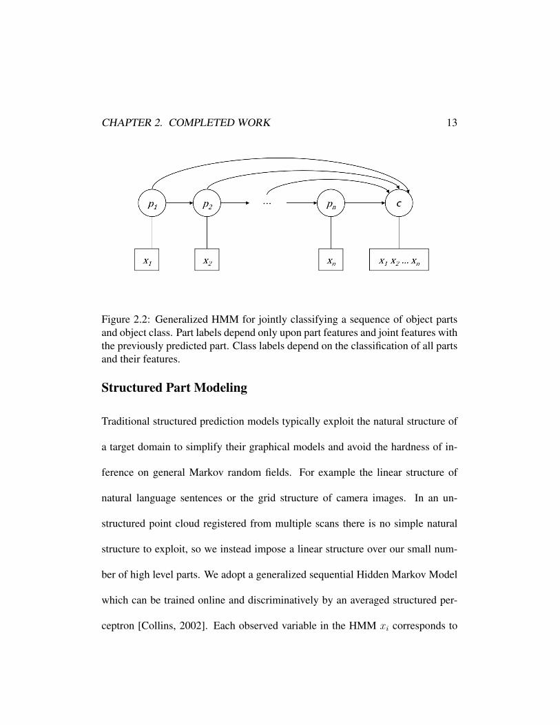
Figure 2.2: Generalized HMM for jointly classifying a sequence of object partsand object class. Part labels depend only upon part features and joint features withthe previously predicted part. Class labels depend on the classification of all partsand their features.
Structured Part Modeling
Traditional structured prediction models typically exploit the natural structure of
a target domain to simplify their graphical models and avoid the hardness of in-
ference on general Markov random fields. For example the linear structure of
natural language sentences or the grid structure of camera images. In an un-
structured point cloud registered from multiple scans there is no simple natural
structure to exploit, so we instead impose a linear structure over our small num-
ber of high level parts. We adopt a generalized sequential Hidden Markov Model
which can be trained online and discriminatively by an averaged structured per-
ceptron [Collins, 2002]. Each observed variable in the HMM xi corresponds to
CHAPTER 2. COMPLETED WORK 14
a part-level feature and the hidden variables correspond to part class labels ai.
The HMM is generalized to include a final hidden variable c corresponding to the
overall object class that depends on all previous observations. A graph depicting
this model can be seen in Figure 2.2.
Our linear approximation to a more general MRF requires a sequential order-
ing of the object parts. While the iterative RANSAC procedure used to generate
the parts gives such an ordering that we found to be superior to random permu-
tations, it is too heavily influenced by variations in occlusions and variable point
density determined by the scanner location. Again we utilize the known geomet-
ric properties of the scene and order the parts such that horizontal parts appear
before vertical parts and within descending order of average height within each
part. This gives an approximate sequential ordering that is more consistent across
all possible objects and allows us to more easily fit our model on a small number
of likely observation sequences.
We also exploit structure by computing additional joint features xi,i−1 between
adjacent parts in the sequential ordering that will be used to learn the pairwise
potentials in the HMM. The features we use here describe the geometric relation-
ships between the two parts and include the dot product between their normals,
the absolute difference in average heights, the distance between part centroids, the
closest distance between points from each part, and a measure of coplanarity as
CHAPTER 2. COMPLETED WORK 15
defined by the mean, median, and max of the cross-fit errors between the points
in one part and the planar estimate of the other.
Part labels for each parts in the sequence are determined by finding the labeling
that maximizes the recursive scoring function
s(ai) = maxai−1
s(ai−1) + p(xi|ai) + p(xi−1,i|ai−1, ai). (2.1)
Where here p(x|Y ) = xTwY , the dot product of the observed features with
the learned model weights for the set of labels Y . Here x may be either the unary
part features or the pairwise features between parts. This recursive function is
maximized by the Viterbi algorithm over the HMM.
The objective to determine the overall object class label c is
maxc
∑i
p(xi|ai, c) +∑i,j
p(xi−1,i|ai−1, ai, c). (2.2)
Note here that terms in this expression include both part and object class labels
and so the estimated weights here are distinct from those used to determine the
part class labels. During training the weight vectors for determining class are
updated only if the corresponding part was correctly classified, otherwise we may
be penalizing the wrong weight vector and convergence of perceptron training
relies on updates only on correctly identified errors. For example, weight wai,c is
CHAPTER 2. COMPLETED WORK 16
updated only if object class c is incorrect but the ith part was correctly classified
as having label ai using weight vector wai and the preceding structure.
Experimental Evaluation
We evaluated our structured prediction model on vehicle point clouds extracted
from the Wright State Ottawa dataset. A total of 222 sedans and SUVs, the two
most commonly occurring vehicle categories, were used in our experiments and
were partitioned into training, development, and testing splits with two-thirds of
the data in training and the remaining equally split between development and test
sets. Two sets of ground truth part labels were generated for this dataset to eval-
uate the unsupervised part segmentation and part level classification. One for the
automatically generated planar part proposals from the RANSAC segmentation
and another large subset with a manual segmentation of the vehicle point clouds
using a 3D labeling tool in order to evaluate the performance of the automatic seg-
mentation. The manual labels include 90 sedans and all 67 SUVs in the dataset
of 222 vehicles. The labels using the unsupervised segmentation include merged
labels like roof-hood and roof-trunk caused by errors in the automatic segmen-
tation. These segmentation errors are generally caused by inclined surfaces with
curved transitions or occlusions that limit the number of points that can be fit. Al-
though generally not planar, interior segments are often extracted for particularly

CHAPTER 2. COMPLETED WORK 17
Classifier Part Acc All AccSVM 76.10 41.50RF 82.44 54.72SP 88.29 56.60Manual SVM 82.18 40.00Manual RF 86.14 50.00Manual SP 93.56 65.00
Table 2.1: Overall part classification results. Part Acc corresponds to the percent-age of correctly classified parts. All Acc is the percentage of vehicles for which allparts are correctly classified. The top rows use the automatic segmentation whilethe bottom rows use the manually segmented data set.
occluded objects with few visible planar parts.
For our baseline we trained support vector machine and random forest clas-
sifiers for part and object classification as well as a simple perceptron for object
classification. When training for part classification these non-structured classi-
fiers used the same part-level feature descriptors as our proposed model but did
not use any of the pairwise features between parts. For object classification we use
a similar set of features defined over the local features of the entire object but not
including any PCA estimation features since our overall objects are not assumed
to be planar and these would vary greatly with occlusion.
Overall part classification results are presented in Table 2.1. By leveraging the
HMM structure and our proposed set of pairwise part-features the structured per-
ceptron classifier is able to consistently ourperform the SVM and random forest
CHAPTER 2. COMPLETED WORK 18
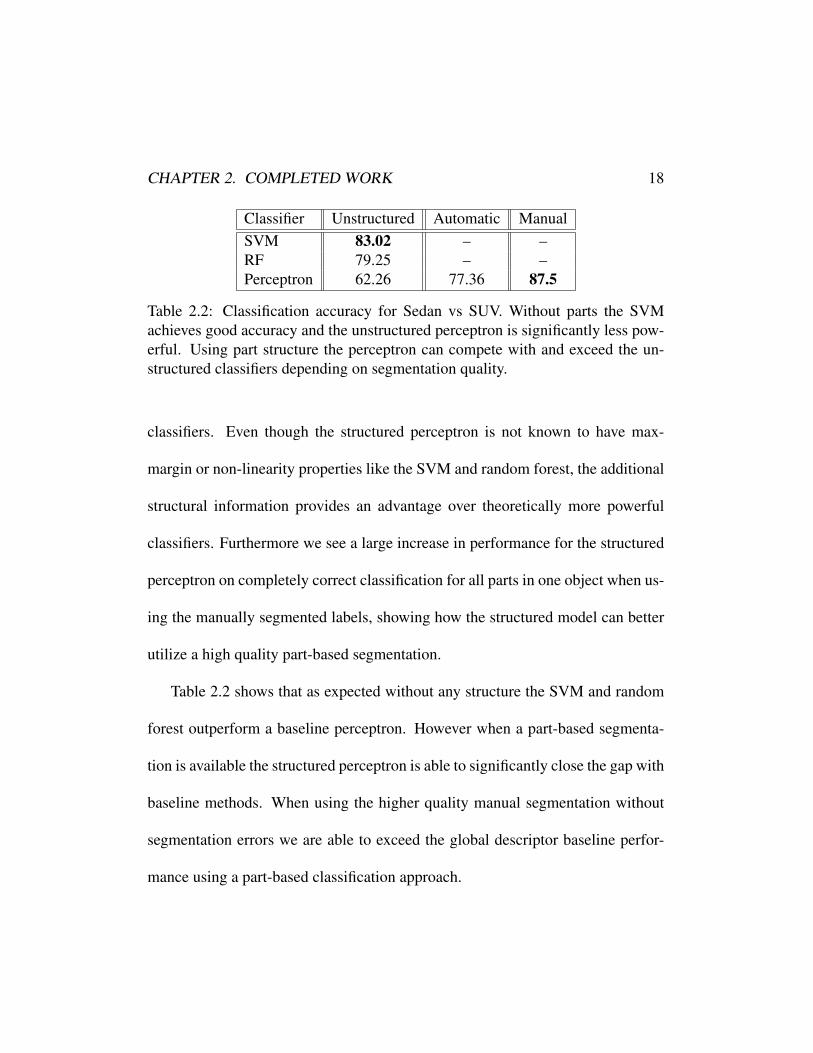
Classifier Unstructured Automatic ManualSVM 83.02 – –RF 79.25 – –Perceptron 62.26 77.36 87.5
Table 2.2: Classification accuracy for Sedan vs SUV. Without parts the SVMachieves good accuracy and the unstructured perceptron is significantly less pow-erful. Using part structure the perceptron can compete with and exceed the un-structured classifiers depending on segmentation quality.
classifiers. Even though the structured perceptron is not known to have max-
margin or non-linearity properties like the SVM and random forest, the additional
structural information provides an advantage over theoretically more powerful
classifiers. Furthermore we see a large increase in performance for the structured
perceptron on completely correct classification for all parts in one object when us-
ing the manually segmented labels, showing how the structured model can better
utilize a high quality part-based segmentation.
Table 2.2 shows that as expected without any structure the SVM and random
forest outperform a baseline perceptron. However when a part-based segmenta-
tion is available the structured perceptron is able to significantly close the gap with
baseline methods. When using the higher quality manual segmentation without
segmentation errors we are able to exceed the global descriptor baseline perfor-
mance using a part-based classification approach.
CHAPTER 2. COMPLETED WORK 19
Conclusion
In this work we presented a part-based structured prediction approach for classify-
ing objects and their semantic parts in unstructured 3D point clouds. Our segmen-
tation algorithm is robust to many of the complexities found in point clouds and
avoids non-surface segments that would be produced by a naive RANSAC seg-
mentation. We evaluated our model on a challenging dataset of partially observed
vehicles from real world LIDAR scans and demonstrated superior performance
over the baseline methods. However we have also identified several challenges
for the model in this work that have motivated us to investigate deep learning
approaches for these tasks.
First, when performing a supervised parts-based classification it is necessary
to generate ground truth labels for every part of every possible object of inter-
est. This is a significant multiplicative increase in labeling efforts which may
not be unique for different choices of part categories or segmentation strategies.
For example here we used approximately planar parts but the labeling may have
to be regenerated if we revised our algorithm to fit curved surfaces. Secondly,
the learned structure is an explicit linear approximation to a more general set of
possible relations between parts that may need to be considered. An informative
pairwise feature may not be found because it does not occur in the predefined ex-
CHAPTER 2. COMPLETED WORK 20
pected ordering. Third, the feature representation has been manually engineered
for extracting geometric information about the parts and their relations in order
to determine overall object class but this does not seem to yield as significant a
gain in performance on the object classification task as the part classification task.
Finally, errors introduced in the unsupervised segmentation impact the classifica-
tion performance and there is no mechanism to adjust the segmentation once it
has been performed.
Deep learning techniques provide a framework to address these challenges in
several ways, both implicitly and explicitly. A deep neural network addresses
the first two challenges by implicitly learning a hierarchical representation of its
inputs [Zeiler and Fergus, 2014], effectively learning features for parts and com-
binations of parts automatically based on the network structure. The challenges
of learning feature representations for solving the target task and correcting errors
introduced earlier in model are also explicitly addressed by end-to-end learning
through the backpropagation algorithm. These considerations led us to move away
from a point cloud representation of our data and develop a convolutional neural
network model that can segment objects in LIDAR range scans.
CHAPTER 2. COMPLETED WORK 21
2.2 CNN-Based Object Segmentation
Object segmentation in LIDAR scenes has previously been studied in point clus-
tering and graph cut based frameworks [Golovinskiy et al., 2009, Dohan et al.,
2015]. Based on the conclusions of our previous work, we take inspiration from
recent work in RGB-D semantic segmentation [Couprie et al., 2013] and apply a
similar convolutional neural network based framework adapted for LIDAR scenes.
In particular we address a relative abundance of missing LIDAR data found in
urban scenes caused by vehicles having reflective paint and refracting glass win-
dows. We show that by labeling missing points in the scanning acquisition grid we
can train our model to achieve a more accurate and complete segmentation mask
for the scene. Additionally, we show that a lightweight set of low-level features,
based on those introduced by [Gupta et al., 2014], that encapsulate the 3D scene
structure computed from the raw LIDAR have a significant effect on performance.
We evaluate our model on a LIDAR dataset collected by Google Street View cars
over large areas of New York City that we have annotated with vehicle labels for
both sensed 3D points and missing LIDAR ray directions.
In the following sections we describe the procedure for generating labels in 3D
images, our preprocessing pipeline for extracting input crops from large LIDAR
scenes, the low-level input features generated for each crop, and the structure of
CHAPTER 2. COMPLETED WORK 22
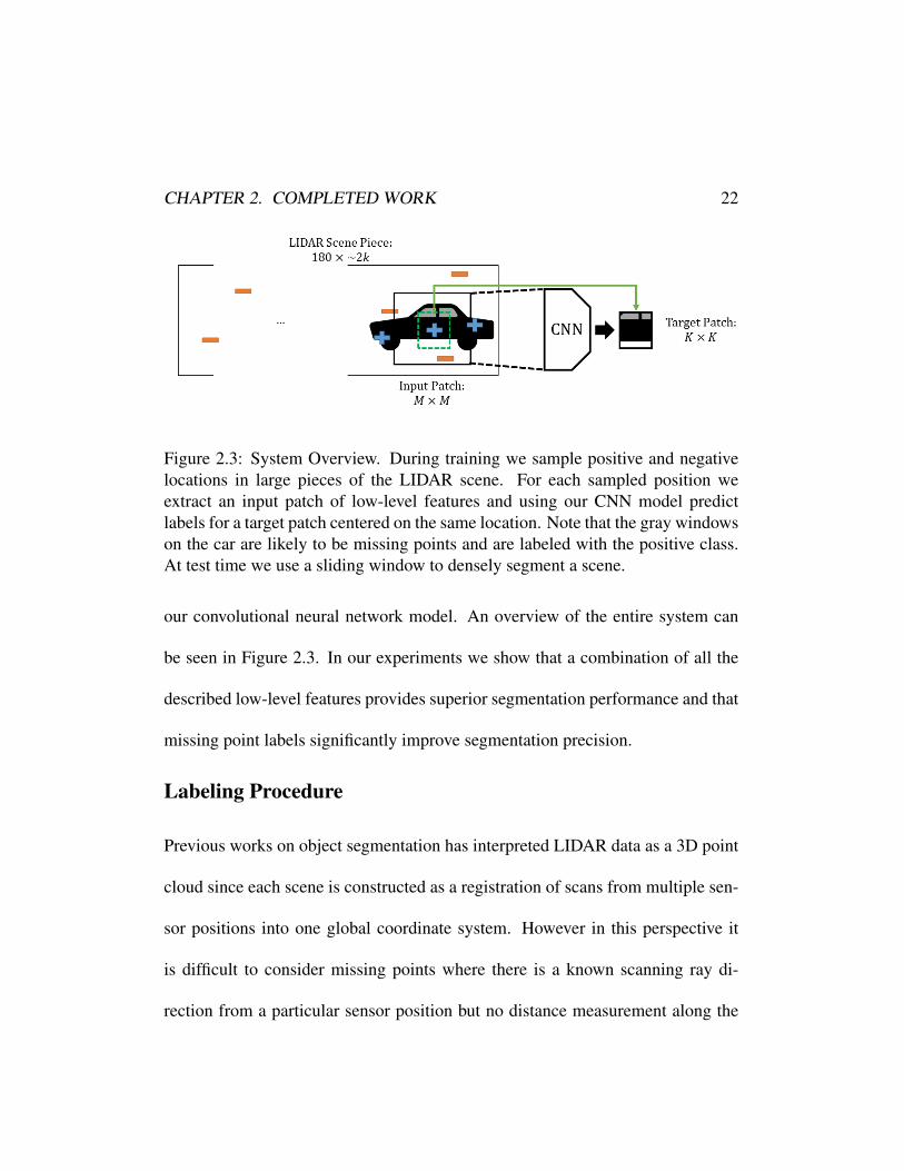
Figure 2.3: System Overview. During training we sample positive and negativelocations in large pieces of the LIDAR scene. For each sampled position weextract an input patch of low-level features and using our CNN model predictlabels for a target patch centered on the same location. Note that the gray windowson the car are likely to be missing points and are labeled with the positive class.At test time we use a sliding window to densely segment a scene.
our convolutional neural network model. An overview of the entire system can
be seen in Figure 2.3. In our experiments we show that a combination of all the
described low-level features provides superior segmentation performance and that
missing point labels significantly improve segmentation precision.
Labeling Procedure
Previous works on object segmentation has interpreted LIDAR data as a 3D point
cloud since each scene is constructed as a registration of scans from multiple sen-
sor positions into one global coordinate system. However in this perspective it
is difficult to consider missing points where there is a known scanning ray di-
rection from a particular sensor position but no distance measurement along the
CHAPTER 2. COMPLETED WORK 23
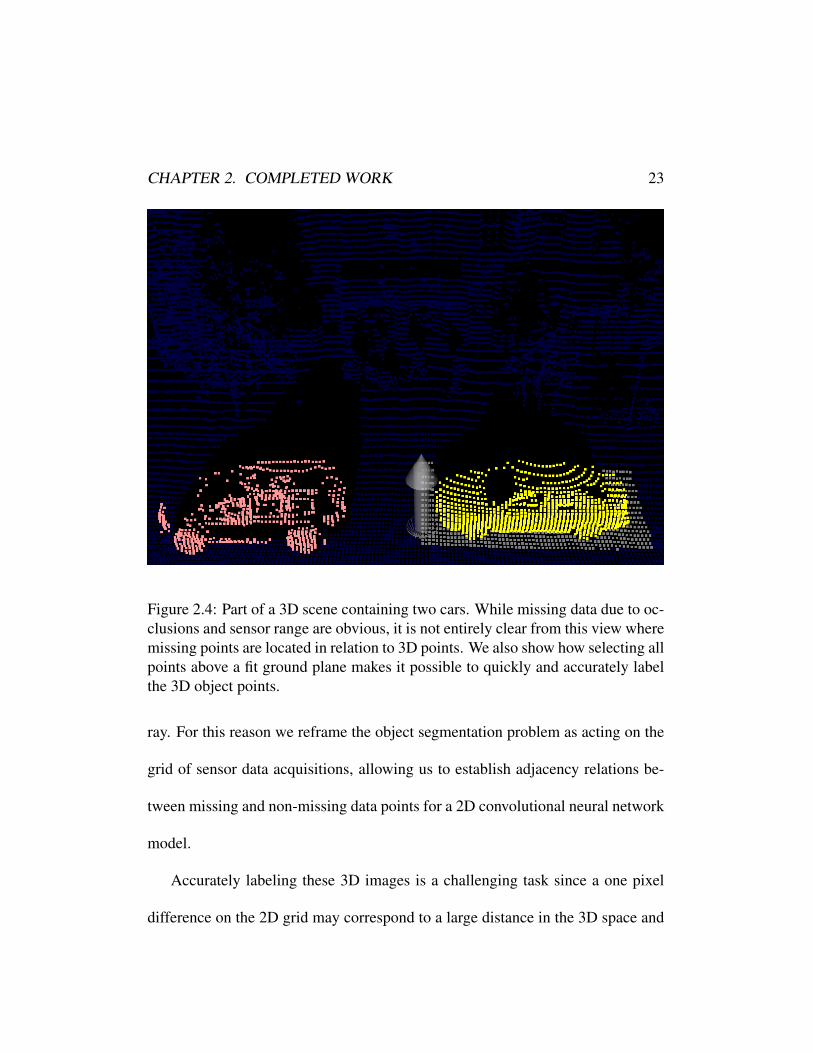
Figure 2.4: Part of a 3D scene containing two cars. While missing data due to oc-clusions and sensor range are obvious, it is not entirely clear from this view wheremissing points are located in relation to 3D points. We also show how selecting allpoints above a fit ground plane makes it possible to quickly and accurately labelthe 3D object points.
ray. For this reason we reframe the object segmentation problem as acting on the
grid of sensor data acquisitions, allowing us to establish adjacency relations be-
tween missing and non-missing data points for a 2D convolutional neural network
model.
Accurately labeling these 3D images is a challenging task since a one pixel
difference on the 2D grid may correspond to a large distance in the 3D space and
CHAPTER 2. COMPLETED WORK 24
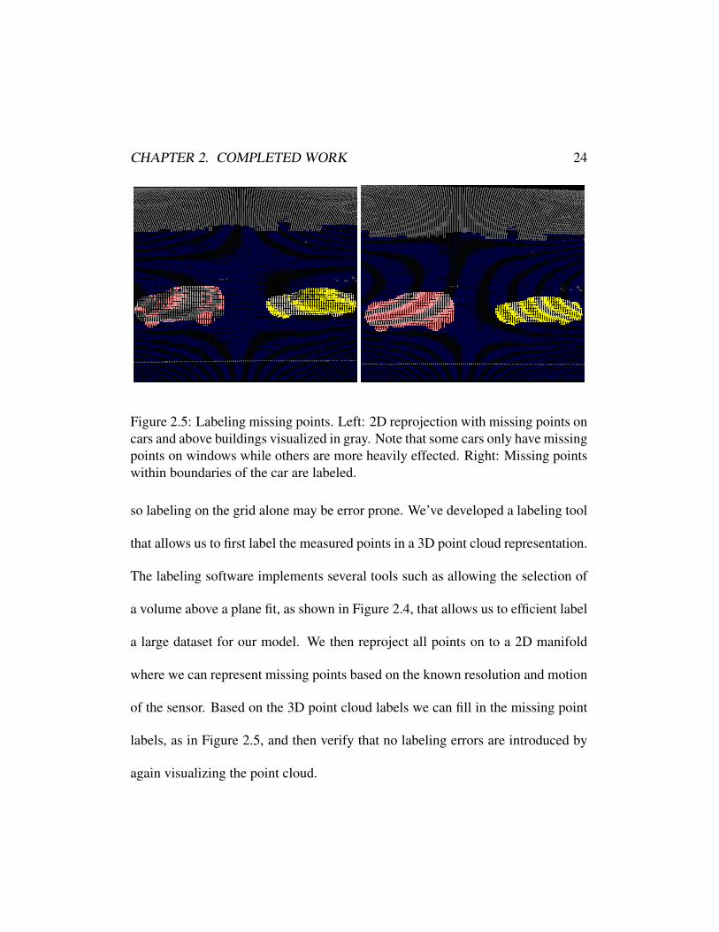
Figure 2.5: Labeling missing points. Left: 2D reprojection with missing points oncars and above buildings visualized in gray. Note that some cars only have missingpoints on windows while others are more heavily effected. Right: Missing pointswithin boundaries of the car are labeled.
so labeling on the grid alone may be error prone. We’ve developed a labeling tool
that allows us to first label the measured points in a 3D point cloud representation.
The labeling software implements several tools such as allowing the selection of
a volume above a plane fit, as shown in Figure 2.4, that allows us to efficient label
a large dataset for our model. We then reproject all points on to a 2D manifold
where we can represent missing points based on the known resolution and motion
of the sensor. Based on the 3D point cloud labels we can fill in the missing point
labels, as in Figure 2.5, and then verify that no labeling errors are introduced by
again visualizing the point cloud.
CHAPTER 2. COMPLETED WORK 25
Patch Sampling
The LIDAR scenes in the Google Street View dataset consist of long runs of con-
tinuous driving by the vehicle the sensors are mounted on resulting in 3D images
that are effectively thousands of scanlines long. These types of images are too
large for a single convolutional neural network. The standard solution for 2D
images of resizing down to a smaller resolution may distort the accurate 3D mea-
surements given by the LIDAR sensor at depth edges and missing point positions.
Rather than simply subdivide each image of our dataset we instead use a random
cropping strategy to generate patches of appropriate size for a CNN that also acts
as data augmentation for training the model.
We first divide each full LIDAR run into smaller pieces of 2 − 4k scanlines,
avoiding segmenting target objects when possible, in order to efficiently label and
preprocess the entire run. During training, for each scene piece we sample N2
unla-
beled background positions and up to N2
labeled object positions depending on the
number of valid positions that yield a full sized patch. This biased sampling helps
approximate a uniform distribution of positive and negative samples for training a
standard classifier, which is necessary in our case since labeled object points are
a minority of scene points.
Centered on each sampled position we generate an M × M patch of input
CHAPTER 2. COMPLETED WORK 26
features and a K×K patch of labels where K ≤M . We typically set K less than
M so that there is sufficient support for features used to predict the object label
and avoid errors due to edge effect. At test time we densely generate patches with
a step size of K to label the entire scene. For training we consider T scene pieces
and define the size of one epoch as NT . We continuously generate new random
patches throughout training, effectively augmenting the size of our dataset without
explicitly storing all possible crops. In order to reduce preprocessing computation
and memory usage we reuse one set of NT samples for a fixed number of training
epochs before generating new samples.
Input Features
Since 3D point positions vary throughout a scene depending on the global coordi-
nate system, it becomes necessary to generate normalized features for each patch
independent of the sampled position. Similar to [Gupta et al., 2014] we generate a
set of features that encode 3D scene structure and properties of the LIDAR sensor.
We consider the depth from the sensor and height along the sensor-up direction as
reliable measures and for each patch generate relative depth and height maps with
respect to the centroid of all points within the patch which gives similar features
for different patches robust to variation in distance from the sensor. These feature
maps are then normalized based on the standard deviations within each patch and
CHAPTER 2. COMPLETED WORK 27
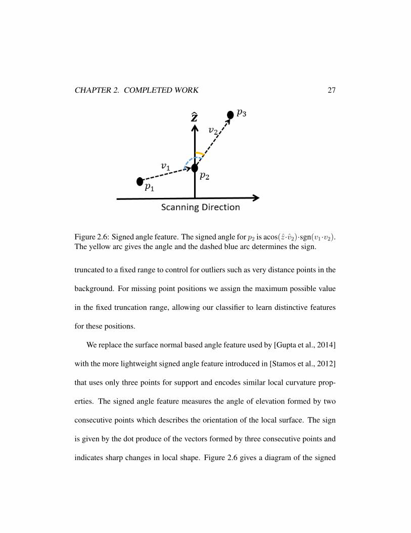
Figure 2.6: Signed angle feature. The signed angle for p2 is acos(z·v2)·sgn(v1·v2).The yellow arc gives the angle and the dashed blue arc determines the sign.
truncated to a fixed range to control for outliers such as very distance points in the
background. For missing point positions we assign the maximum possible value
in the fixed truncation range, allowing our classifier to learn distinctive features
for these positions.
We replace the surface normal based angle feature used by [Gupta et al., 2014]
with the more lightweight signed angle feature introduced in [Stamos et al., 2012]
that uses only three points for support and encodes similar local curvature prop-
erties. The signed angle feature measures the angle of elevation formed by two
consecutive points which describes the orientation of the local surface. The sign
is given by the dot produce of the vectors formed by three consecutive points and
indicates sharp changes in local shape. Figure 2.6 gives a diagram of the signed
CHAPTER 2. COMPLETED WORK 28
angle definition.
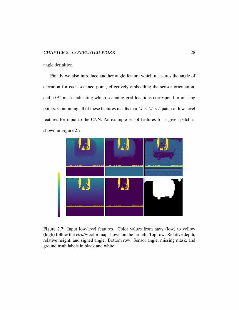
Finally we also introduce another angle feature which measures the angle of
elevation for each scanned point, effectively embedding the sensor orientation,
and a 0/1 mask indicating which scanning grid locations correspond to missing
points. Combining all of these features results in a M ×M × 5 patch of low-level
features for input to the CNN. An example set of features for a given patch is
shown in Figure 2.7.
Figure 2.7: Input low-level features. Color values from navy (low) to yellow(high) follow the viridis color map shown on the far left. Top row: Relative depth,relative height, and signed angle. Bottom row: Sensor angle, missing mask, andground truth labels in black and white.
CHAPTER 2. COMPLETED WORK 29
CNN Model
Our model follows a commonly used architecture for convolutional neural net-
works that consists of a sequence of convolutional layers with the ReLU activation
function and max-pooling followed by a sequence of fully connected linear layers.
We set the number of layers to two 5×5 convolutional with 2×2 max-pooling and
two linear layers. This model is relatively shallow compared to modern state-of-
the-art 2D image models, but this design was useful in establishing a baseline for
LIDAR data and serving as a testbed for our preprocessing pipeline and different
combinations of low-level input features.
In order to accomplish single class segmentation our model predicts a K ×K
block of labels for a window of points centered on the M ×M input patch. We
parameterize this as K2 independent binary classification tasks utilizing logistic
regression on the representation for the entire patch produced by the final layer of
the CNN. The total loss of the model is the sum of the binary cross entropy losses
for each logistic regression plus an L2-regularization penalty on the weights of
the fully connected layers,
−K2∑k=1
yk log(pk) + (1− yk) log(1− pk) +λ
2
L∑l=1
||Wl||22, (2.3)
where yk is 1 if the kth point in the target grid is positive and 0 otherwise, pk
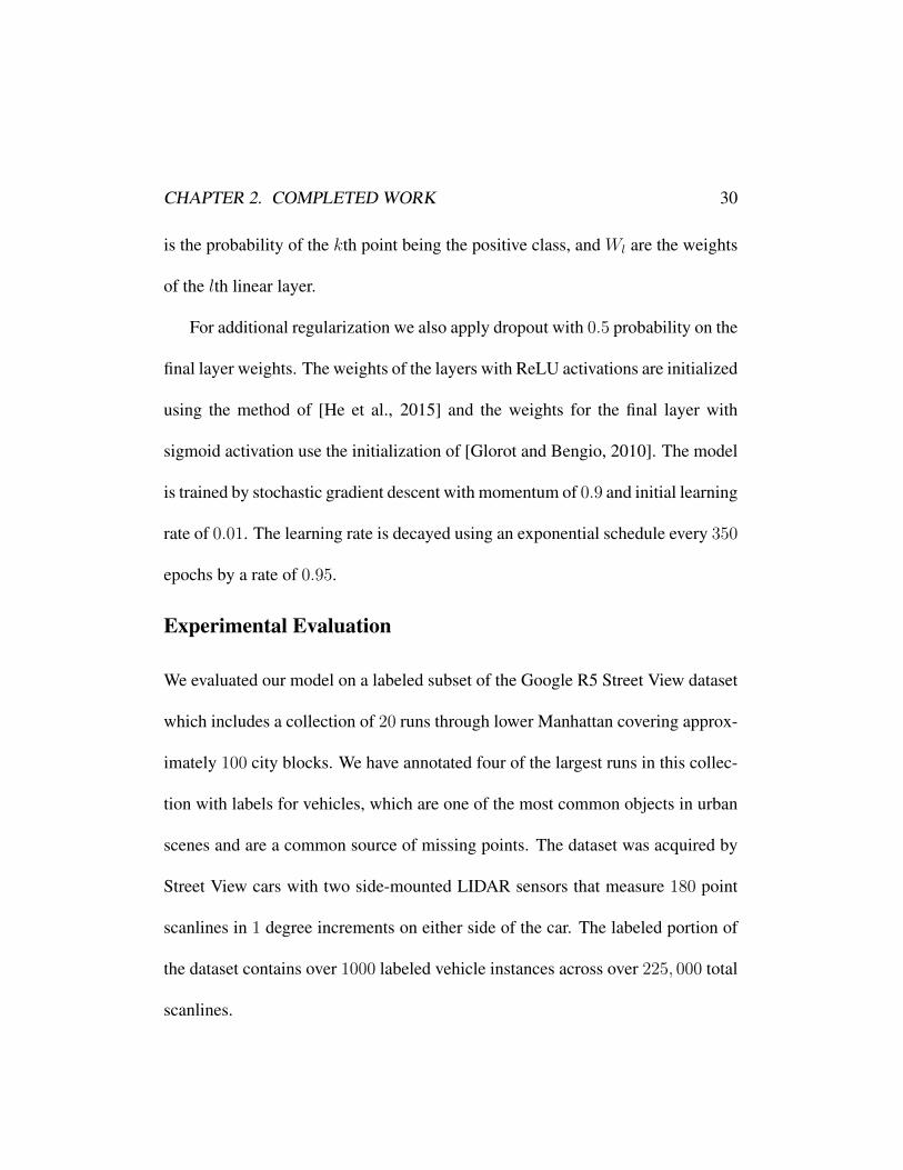
CHAPTER 2. COMPLETED WORK 30
is the probability of the kth point being the positive class, and Wl are the weights
of the lth linear layer.
For additional regularization we also apply dropout with 0.5 probability on the
final layer weights. The weights of the layers with ReLU activations are initialized
using the method of [He et al., 2015] and the weights for the final layer with
sigmoid activation use the initialization of [Glorot and Bengio, 2010]. The model
is trained by stochastic gradient descent with momentum of 0.9 and initial learning
rate of 0.01. The learning rate is decayed using an exponential schedule every 350
epochs by a rate of 0.95.
Experimental Evaluation
We evaluated our model on a labeled subset of the Google R5 Street View dataset
which includes a collection of 20 runs through lower Manhattan covering approx-
imately 100 city blocks. We have annotated four of the largest runs in this collec-
tion with labels for vehicles, which are one of the most common objects in urban
scenes and are a common source of missing points. The dataset was acquired by
Street View cars with two side-mounted LIDAR sensors that measure 180 point
scanlines in 1 degree increments on either side of the car. The labeled portion of
the dataset contains over 1000 labeled vehicle instances across over 225, 000 total
scanlines.
CHAPTER 2. COMPLETED WORK 31
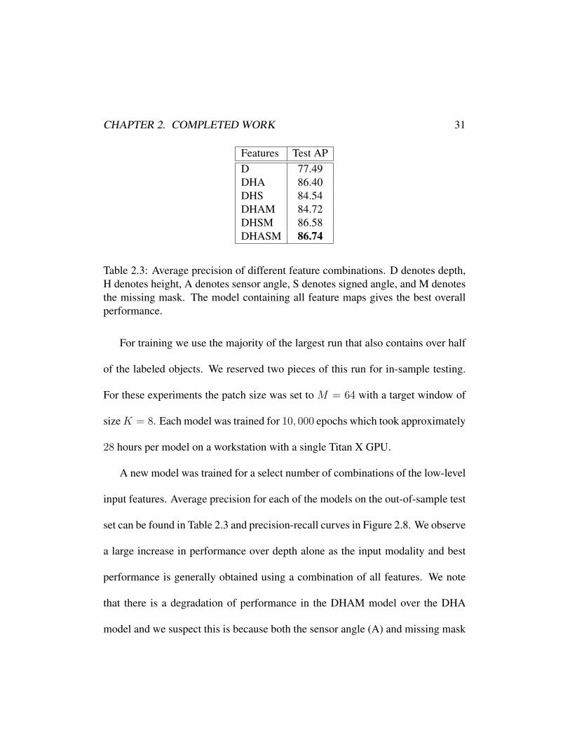
Features Test APD 77.49DHA 86.40DHS 84.54DHAM 84.72DHSM 86.58DHASM 86.74
Table 2.3: Average precision of different feature combinations. D denotes depth,H denotes height, A denotes sensor angle, S denotes signed angle, and M denotesthe missing mask. The model containing all feature maps gives the best overallperformance.
For training we use the majority of the largest run that also contains over half
of the labeled objects. We reserved two pieces of this run for in-sample testing.
For these experiments the patch size was set to M = 64 with a target window of
sizeK = 8. Each model was trained for 10, 000 epochs which took approximately
28 hours per model on a workstation with a single Titan X GPU.
A new model was trained for a select number of combinations of the low-level
input features. Average precision for each of the models on the out-of-sample test
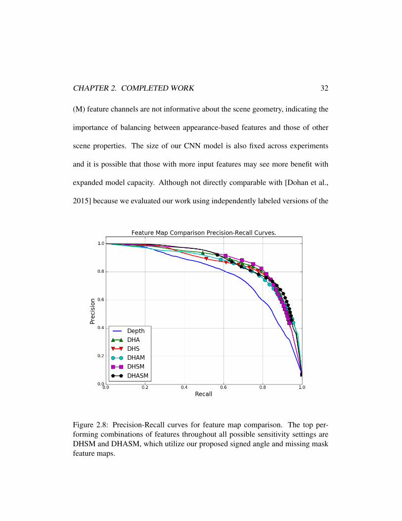
set can be found in Table 2.3 and precision-recall curves in Figure 2.8. We observe
a large increase in performance over depth alone as the input modality and best
performance is generally obtained using a combination of all features. We note
that there is a degradation of performance in the DHAM model over the DHA
model and we suspect this is because both the sensor angle (A) and missing mask
CHAPTER 2. COMPLETED WORK 32
(M) feature channels are not informative about the scene geometry, indicating the
importance of balancing between appearance-based features and those of other
scene properties. The size of our CNN model is also fixed across experiments
and it is possible that those with more input features may see more benefit with
expanded model capacity. Although not directly comparable with [Dohan et al.,
2015] because we evaluated our work using independently labeled versions of the
Figure 2.8: Precision-Recall curves for feature map comparison. The top per-forming combinations of features throughout all possible sensitivity settings areDHSM and DHASM, which utilize our proposed signed angle and missing maskfeature maps.
CHAPTER 2. COMPLETED WORK 33
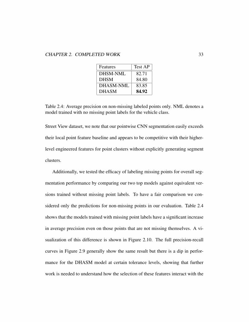
Features Test APDHSM-NML 82.71DHSM 84.80DHASM-NML 83.85DHASM 84.92
Table 2.4: Average precision on non-missing labeled points only. NML denotes amodel trained with no missing point labels for the vehicle class.
Street View dataset, we note that our pointwise CNN segmentation easily exceeds
their local point feature baseline and appears to be competitive with their higher-
level engineered features for point clusters without explicitly generating segment
clusters.
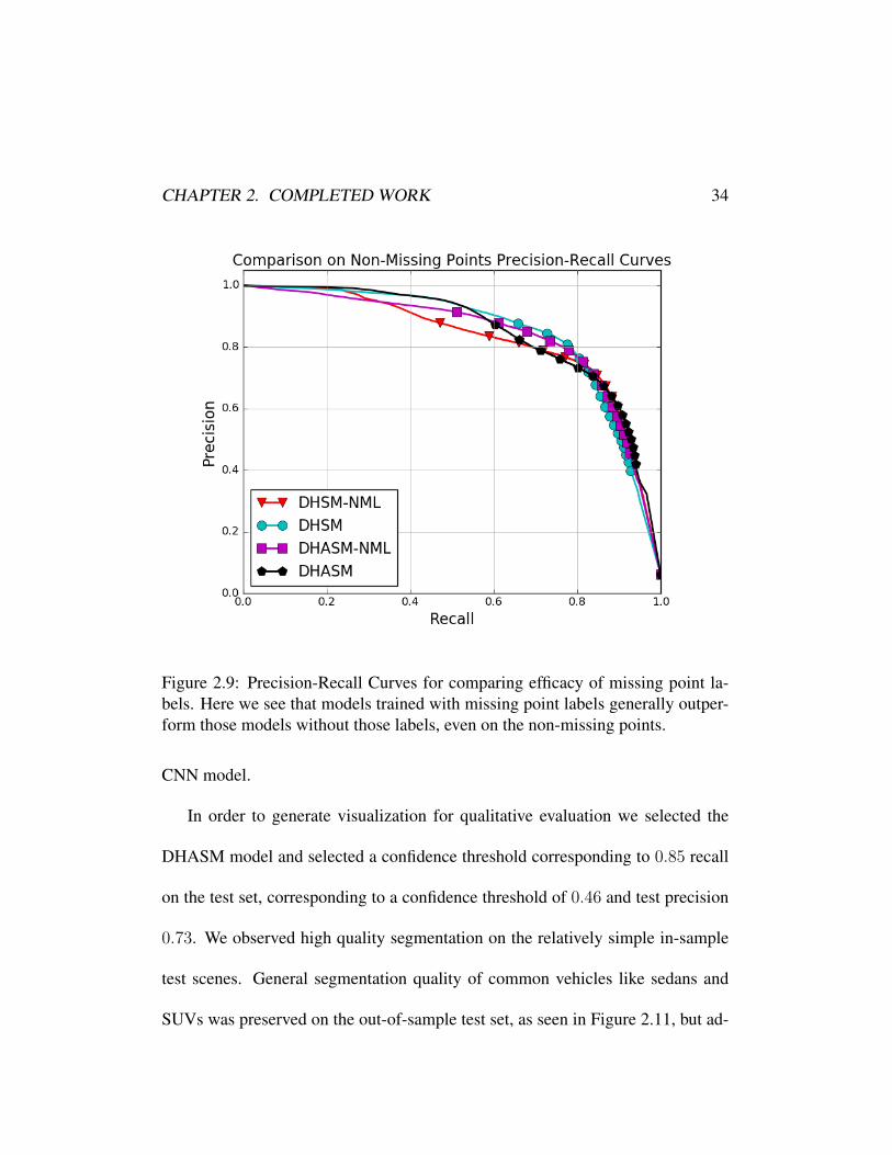
Additionally, we tested the efficacy of labeling missing points for overall seg-
mentation performance by comparing our two top models against equivalent ver-
sions trained without missing point labels. To have a fair comparison we con-
sidered only the predictions for non-missing points in our evaluation. Table 2.4
shows that the models trained with missing point labels have a significant increase
in average precision even on those points that are not missing themselves. A vi-
sualization of this difference is shown in Figure 2.10. The full precision-recall
curves in Figure 2.9 generally show the same result but there is a dip in perfor-
mance for the DHASM model at certain tolerance levels, showing that further
work is needed to understand how the selection of these features interact with the
CHAPTER 2. COMPLETED WORK 34
Figure 2.9: Precision-Recall Curves for comparing efficacy of missing point la-bels. Here we see that models trained with missing point labels generally outper-form those models without those labels, even on the non-missing points.
CNN model.
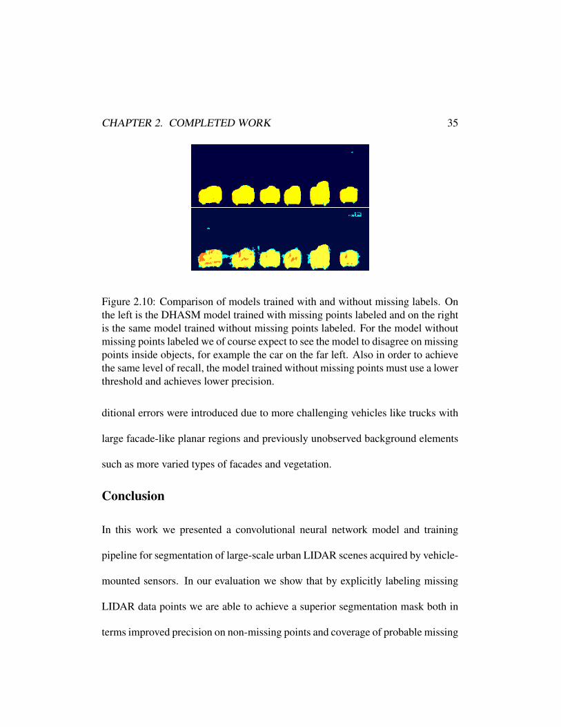
In order to generate visualization for qualitative evaluation we selected the
DHASM model and selected a confidence threshold corresponding to 0.85 recall
on the test set, corresponding to a confidence threshold of 0.46 and test precision
0.73. We observed high quality segmentation on the relatively simple in-sample
test scenes. General segmentation quality of common vehicles like sedans and
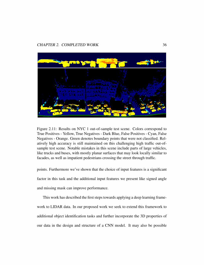
SUVs was preserved on the out-of-sample test set, as seen in Figure 2.11, but ad-
CHAPTER 2. COMPLETED WORK 35
Figure 2.10: Comparison of models trained with and without missing labels. Onthe left is the DHASM model trained with missing points labeled and on the rightis the same model trained without missing points labeled. For the model withoutmissing points labeled we of course expect to see the model to disagree on missingpoints inside objects, for example the car on the far left. Also in order to achievethe same level of recall, the model trained without missing points must use a lowerthreshold and achieves lower precision.
ditional errors were introduced due to more challenging vehicles like trucks with
large facade-like planar regions and previously unobserved background elements
such as more varied types of facades and vegetation.
Conclusion
In this work we presented a convolutional neural network model and training
pipeline for segmentation of large-scale urban LIDAR scenes acquired by vehicle-
mounted sensors. In our evaluation we show that by explicitly labeling missing
LIDAR data points we are able to achieve a superior segmentation mask both in
terms improved precision on non-missing points and coverage of probable missing
CHAPTER 2. COMPLETED WORK 36
Figure 2.11: Results on NYC 1 out-of-sample test scene. Colors correspond toTrue Positives - Yellow, True Negatives - Dark Blue, False Positives - Cyan, FalseNegatives - Orange. Green denotes boundary points that were not classified. Rel-atively high accuracy is still maintained on this challenging high traffic out-of-sample test scene. Notable mistakes in this scene include parts of large vehicles,like trucks and buses, with mostly planar surfaces that may look locally similar tofacades, as well as impatient pedestrians crossing the street through traffic.
points. Furthermore we’ve shown that the choice of input features is a significant
factor in this task and the additional input features we present like signed angle
and missing mask can improve performance.
This work has described the first steps towards applying a deep learning frame-
work to LIDAR data. In our proposed work we seek to extend this framework to
additional object identification tasks and further incorporate the 3D properties of
our data in the design and structure of a CNN model. It may also be possible
CHAPTER 2. COMPLETED WORK 37
to impute expected depth values for missing points in the same way we predict
their semantic labels, however this would require measuring ground truth values
in controlled scans or the use of synthetic data.
2.3 Related Work
While there has been some additional work in the direction of 3D point clustering
methods for object segmentation and classification [Dohan et al., 2015], the body
of work that has received more attention and is most related to our proposed work
lies at the intersection of 3D computer vision and deep machine learning. Not
all of these works focus on the object identification tasks or utilize 3D sensors
for input, but they share common deep learning methodologies and relate their
given task to the 3D world and as such may influence our proposed work. We
shall primarily describe recent work on object identification in 3D images which
is most closely related to our proposal and also briefly survey work on other 3D
vision tasks including estimation of 3D properties in 2D images.
Initial work within the recent wave of deep learning in 3D images utilized
RGB-D sensors and treated depth as simply an additional input modality for
semantic segmentation with 2D convolutional neural networks [Couprie et al.,
2013]. However depth alone does not entirely capture all the geometric proper-
ties of the image. For example a pair of adjacent pixels in a depth image may
CHAPTER 2. COMPLETED WORK 38
have the same value but may be further apart in space than another pair of iden-
tical pixels closer to the sensor. In this case determining the actual 3D positions
of these points requires knowledge of the sensor’s spatial resolution. The work
of [Gupta et al., 2014] addresses this by computing additional features during
preprocessing which include height from an estimated ground plane and angle be-
tween estimated surface normals and the up direction to generate CNN features
for object detection, although like many other works from this period the CNN
is used primarily as a feature extractor rather than for end-to-end learning. An
earlier work on object pose estimation [Papon and Schoeler, 2015] utilized known
surface normals themselves as additional input channels from synthetic RGB-D
images which were used because large datasets with pose annotations were not
yet available. A related line of work in 2D vision has used RGB-D images as
ground truth for estimating depth and surface normals as well as semantic labels
in RGB images [Eigen and Fergus, 2015, Mousavian et al., 2016], and has also
been extended to use these estimates for predicting object pose and visual sim-
ilarity between objects [Bansal et al., 2016]. One unifying theme in all of these
works is that low-level geometric properties like depth and surface normals are re-
lated to higher level tasks like object pose estimation and semantic segmentation
and can be utilized either as pre-calculated inputs or auxiliary outputs to improve
performance on these tasks.
CHAPTER 2. COMPLETED WORK 39
Another branch of 3D deep learning for object recognition considers objects as
existing in a 3D space rather than lying on a 3D image and generates feature rep-
resentations based on this perspective. For example, given a 3D object model the
work of [Shi et al., 2015] generates a 2D convolutional feature map by projecting
points from the object onto an enclosing cylinder. This is related to a multi-view
approach like that of [Su et al., 2015] which generates a representation by pooling
2D convolutional features from multiple viewpoints surrounding the object. An
alternative approach is to represent the objects using a 3D voxel grid, this is used
by [Wu et al., 2015] as input to a 3D convolutional neural network for shape com-
pletion and object recognition as well as view planning for active recognition. A
similar 3D convolutional framework is used by [Song and Xiao, 2016] for 3D re-
gion proposal and combined with 2D image features for object classification and
3D bounding box refinement. Both volumetric and multi-view approaches are ex-
amined by [Qi et al., 2016] where they note a surprising performance shortfall of
3D voxel methods. These methods are sensitive to the choice of grid orientation
and are more constrained in terms of the spatial resolution that can be represented
since memory requirements grow cubically rather than quadratically in the size
of the representation. They propose several solutions such as multiple volumetric
inputs with various orientations of the 3D input. They also utilize probing kernels
which are 1×1×N convolutional kernels, whereN is the full volume extent, that

CHAPTER 2. COMPLETED WORK 40
transform the input volume into an image representation which is then processed
by 2D convolutions. Overall this line of work is promising for its ability to pro-
cess more complete 3D data and learn more fine-grained 3D relations in densely
packed 3D scenes, but further work is needed to enable efficient high resolution
representations and robustness to variations in object pose.

Chapter 3
Proposed Work
Motivated by earlier work on multitask learning [Caruana, 1998, Collobert and
Weston, 2008] and the recent success of joint localization and segmentation sys-
tems, we propose a model for joint object localization, segmentation, classifica-
tion, and pose estimation in 3D images. We identify these as the set of basic tasks
necessary for higher level applications involving objects of interest in a 3D envi-
ronment. Our proposed model will be based on several recent innovations in neu-
ral network component design including fully convolutional networks [Long et al.,
2015], region proposal networks [Ren et al., 2015], spatial transformers [Jaderberg
et al., 2015], and sub-pixel convolutions [Shi et al., 2016].
To reasonably limit the scope of this proposed work we impose the following
restrictions which will be reserved for future work, note however that we consider
the proposed work as a necessary prerequisite for the tasks we exclude. In this
proposal we limit ourselves to single 3D image data such as a RGB-D camera
41
CHAPTER 3. PROPOSED WORK 42
frame or a single sweep of LIDAR scanlines. This excludes both video sequences
of 3D images and densely registered 3D scenes from multiple views as possible
data sources. We also exclude the task of complete shape reconstruction since
it typically requires multiple views, reference database matching, or a generative
model and it may be a significantly more resource intensive task that would limit
the practical design of our model. Although, we may still consider the task of
reconstructing missing data points that should have been visible by the sensor but
were not measured due to limitations of the active sensing technology.
We intend to continue using the Google Street View dataset that was used in
our previous work and will further extend it with oriented bounding boxes that
capture the pose for each object. Additionally, we’ve investigated publicly avail-
able 3D datasets in the urban LIDAR and indoor RGB-D settings. The KITTI
dataset [Geiger et al., 2013] is a benchmark dataset for autonomous driving and
contains oriented 3D bounding boxes for objects on the road such as cars, trucks,
and pedestrians. Unfortunately the KITTI dataset does not contain an official se-
mantic segmentation benchmark but there are some annotated subsets of the data
that we may use. Synthia [Ros et al., 2016] is a large scale synthetic dataset for
semantic segmentation of urban scenes, however it does not appear to include ob-
ject pose annotations. Because of these limitations if we were to use these datasets
for training we would consider combining them with domain adaptation [Ganin
CHAPTER 3. PROPOSED WORK 43
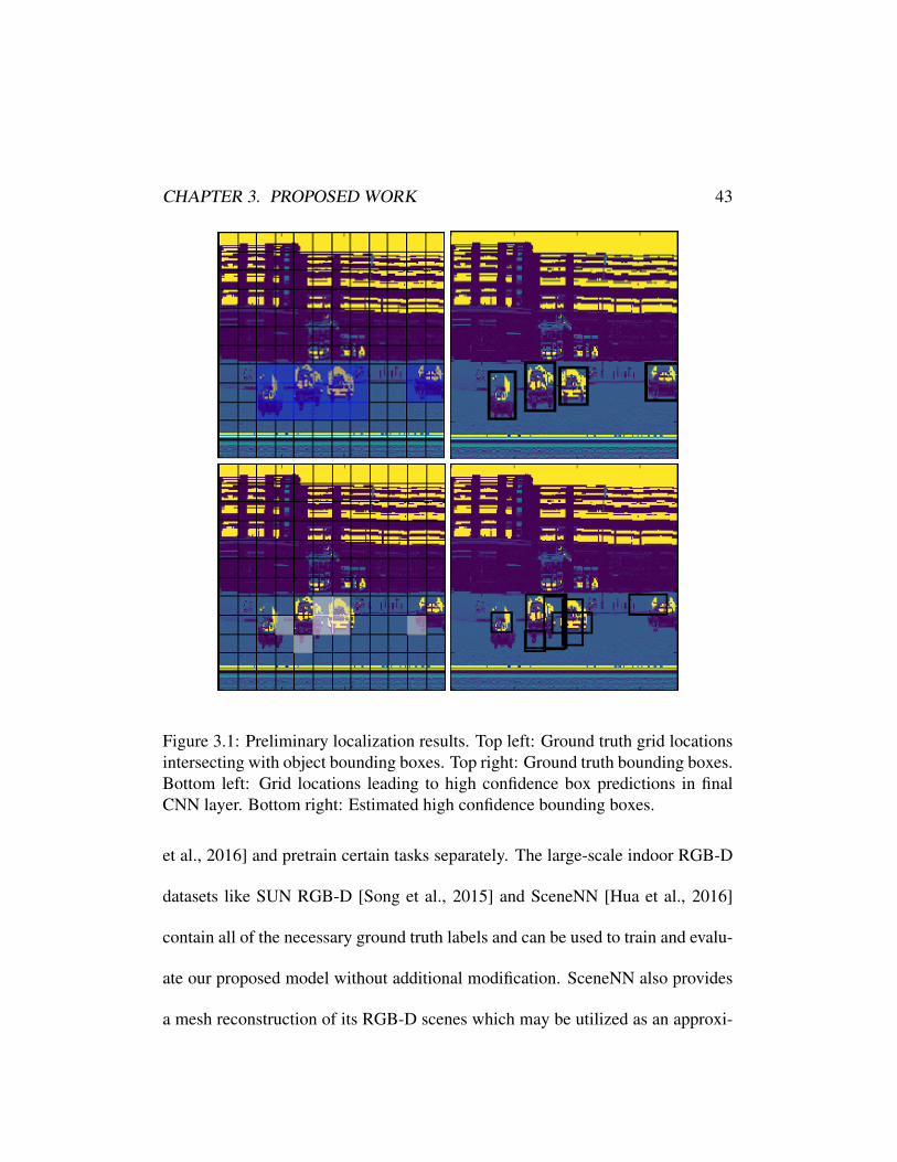
Figure 3.1: Preliminary localization results. Top left: Ground truth grid locationsintersecting with object bounding boxes. Top right: Ground truth bounding boxes.Bottom left: Grid locations leading to high confidence box predictions in finalCNN layer. Bottom right: Estimated high confidence bounding boxes.
et al., 2016] and pretrain certain tasks separately. The large-scale indoor RGB-D
datasets like SUN RGB-D [Song et al., 2015] and SceneNN [Hua et al., 2016]
contain all of the necessary ground truth labels and can be used to train and evalu-
ate our proposed model without additional modification. SceneNN also provides
a mesh reconstruction of its RGB-D scenes which may be utilized as an approxi-
CHAPTER 3. PROPOSED WORK 44
mate ground truth for missing point estimation.
For our baselines we will build independent convolutional neural network
models for each of the tasks based on efficient model architectures that compete
with the state-of-the-art, for example our previous work for segmentation or the
YOLO localization and classification network [Redmon et al., 2016] for which
we have already implemented a fully convolutional variant for 2D bounding box
estimation with preliminary results shown in Figure 3.1. For 3D images we will
extend this localization to predict axis-aligned 3D bounding boxes. Either the out-
put of the baseline localization network or random crops based on ground truth
labels may be used as the input for classification, segmentation, and object pose
estimation baselines.
Although we expect to see a benefit in the shared representation of a network
that jointly solves the object identification tasks, we note that the state-of-the-
art networks for these tasks have architectures that have been specialized in sig-
nificantly different ways. For example, classification networks typically contain
many pooling layers for translation invariance and produce a low dimensional
representation for the likelihood of each class whereas the performance of seg-
mentation networks degrade with excessive pooling and the output needs to have
the same spatial dimensions as the input image. Our strategy to address these con-
cerns is to design our network to prioritize an accurate instance-level segmentation
CHAPTER 3. PROPOSED WORK 45
which may be most useful for upstream tasks while mitigating potential shortfalls
for other tasks with specialized branches from the main computational path. To
that end we’ve identified several recent innovations in neural network design that
can aid in this goal and also have interesting implications for adaptation to 3D
images.
section*Localization in Depth
One of the main tasks in the pipeline is localization since some scenes are
sparsely populated with objects and so it is beneficial to further process only those
regions where an object has been localized for the remaining tasks. Previously
localization has been performed in two stages, region proposal where candidate
locations are generated either through an external method or a region proposal
network, and then object detection where the features from the proposed region
are used to predict confidence in an object’s presence in the region as well as a
more refined bounding box containing the object. Such an approach can be found
in the Deep Sliding Shapes architecture [Song and Xiao, 2016] which has a region
proposal network with the property that proposals of different scales are generated
based on representations from different layers of the work. Architectures like
YOLO and Single Shot Detector [Liu et al., 2016] attempt to avoid region proposal
entirely, however SSD uses the same idea as Deep Sliding Shapes and generates
multiple localizations after each downsampling step in the CNN. For this proposal
CHAPTER 3. PROPOSED WORK 46
we would like to investigate a localization method that adapts this idea to 3D
images by predicting proposals at multiple depths as well as scales throughout
the network. Rather than adopt a full 3D volumetric approach we will instead
partition the observed viewing volume into slices along the depth direction and
associate each ground truth location with overlapping slices. The network will
still perform efficient 2D convolutions but will be expected to predict a confidence
and location for each depth slice as well as each spatial grid cell. We expect this
depth conditional approach to separate objects that overlap in the 2D projection
and better estimate 3D locations.
Spatial Transformers for Pose Estimation
There has been some prior work in 3D pose estimation, including a recent ex-
tension of the Single Shot Detector [Poirson et al., 2016], and one of the most
promising approaches is that of the Spatial Transformer Network [Jaderberg et al.,
2015]. Unlike other approaches that take the resulting features from a localization
network and directly predict the pose of the localized object, the STN generates
an affine transformation for the coordinates of a sampling grid on the input feature
map. When applied to an input image this transformation tends to both localize
an object of interest and transform the object to a pose that is helpful for optimiz-
ing the network objective. For classification networks this tends to be a canonical
CHAPTER 3. PROPOSED WORK 47
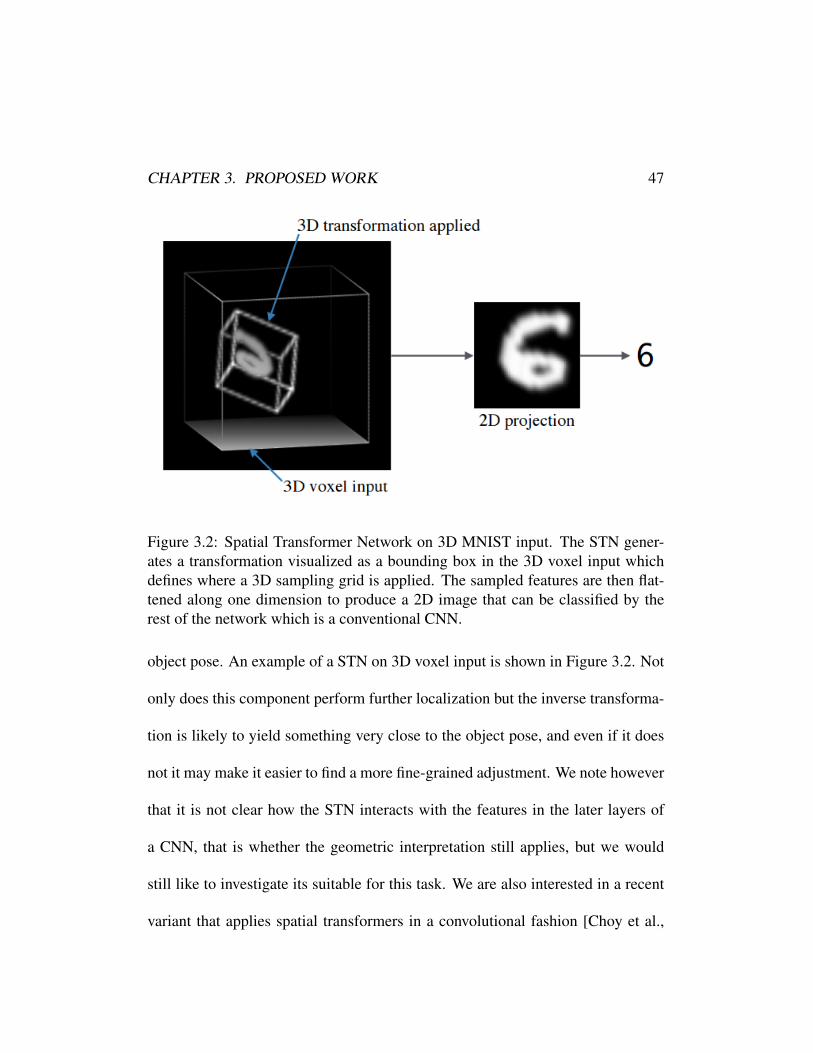
Figure 3.2: Spatial Transformer Network on 3D MNIST input. The STN gener-ates a transformation visualized as a bounding box in the 3D voxel input whichdefines where a 3D sampling grid is applied. The sampled features are then flat-tened along one dimension to produce a 2D image that can be classified by therest of the network which is a conventional CNN.
object pose. An example of a STN on 3D voxel input is shown in Figure 3.2. Not
only does this component perform further localization but the inverse transforma-
tion is likely to yield something very close to the object pose, and even if it does
not it may make it easier to find a more fine-grained adjustment. We note however
that it is not clear how the STN interacts with the features in the later layers of
a CNN, that is whether the geometric interpretation still applies, but we would
still like to investigate its suitable for this task. We are also interested in a recent
variant that applies spatial transformers in a convolutional fashion [Choy et al.,
CHAPTER 3. PROPOSED WORK 48
2016], allowing for many transformations on a single feature map.
Subpixel Methods for Segmentation and Detection
Fully convolutional neural networks with up-sampling convolutions [Long et al.,
2015] have had a big impact on the segmentation literature, allowing architectures
that effectively reverse the pooling operations of a traditional CNN and allow for
outputs as large as the input or even larger. More recently it has been established
in work on image super-resolution [Shi et al., 2016] and depth estimation [Laina
et al., 2016] that the 2D up-sampling convolution operation is equivalent to a
regular convolution with cr2 feature channels where c is the original number of
feature channels and r is the up-sampling ratio. The resulting cr2 feature map
can be efficiently reshuffled to have the same size as the target output. Effectively
each channel contains information on surrounding subpixels in the spatial feature
map. A similar idea has been applied to instance segmentation and detection [Dai
et al., 2016a, Dai et al., 2016c] that associates certain features in each grid cell of
the final convolutional layer with a higher resolution score map for each possible
location. In our work we would like to adopt this approach for segmentation and
investigate whether we can establish a similar relationship in 3D images between
depth slices without explicitly representing our data in a 3D volumetric form.
CHAPTER 3. PROPOSED WORK 49
3.1 Timeline for Completion
Table 3.1 contains a schedule for the completion of the tasks outlined in this
proposal. We are targeting the March deadline for ICCV for our initial confer-
ence submission of this work. This submission should include a complete model
for joint localization, segmentation, classification, and pose estimation as well as
evaluation on the Google Street View and at least one other dataset. Realistically
there is probably not enough time to implement and train models for all of the
three proposed experimental directions for this deadline but ideally at least one of
these will be part of the submission.
Optimistically we will be able to revisit the tasks of domain adaptation and
missing point reconstruction for a follow-up paper that will be submitted to 3DV
in Summer 2017. Otherwise we will continue work on our earlier proposed ex-
periments for the 3DV submission and the dissertation.

CHAPTER 3. PROPOSED WORK 50
Date MilestonesDecember 2016 Prepare KITTI, Synthia, SUN RGB-D, and SceneNN datasets for use.
Annotate Street View dataset with object bounding boxes.Begin implementation of baselines for classification, localization, andpose estimation.
January 2017 Complete implementation of baseline models and begin training mod-els for evaluation.Implement joint localization, segmentation, classification, and poseestimation model.
February 2017 Experiment with architectures using spatial partitioning of viewingvolume, spatial transformers, and sub-pixel shuffle techniques.
March 2017 Prepare paper for submission to ICCV 2017.Additional experiments on domain adaptation and missing point re-construction.
April 2017 Dissertation writing.Prepare paper submission to 3DV 2017.
May 2017 Dissertation defense.
Table 3.1: Schedule for completion of tasks.

Bibliography
[Anand et al., 2013] Anand, A., Koppula, H. S., Joachims, T., and Saxena,A. (2013). Contextually guided semantic labeling and search for three-dimensional point clouds. The International Journal of Robotics Research,32(1):19–34.
[Bansal et al., 2016] Bansal, A., Russell, B., and Gupta, A. (2016). Marr Revis-ited: 2D-3D model alignment via surface normal prediction. In CVPR.
[Barber et al., 1996] Barber, C. B., Dobkin, D. P., and Huhdanpaa, H. (1996).The quickhull algorithm for convex hulls. ACM Transactions on MathematicalSoftware (TOMS), 22(4):469–483.
[Caruana, 1998] Caruana, R. (1998). Multitask learning. In Learning to learn,pages 95–133. Springer.
[Choy et al., 2016] Choy, C. B., Chandraker, M., Gwak, J., and Savarese, S.(2016). Universal correspondence network. In Advances In Neural InformationProcessing Systems, pages 2406–2414.
[Collins, 2002] Collins, M. (2002). Discriminative training methods for hiddenmarkov models: Theory and experiments with perceptron algorithms. In Pro-ceedings of the ACL-02 conference on Empirical methods in natural languageprocessing-Volume 10, pages 1–8. Association for Computational Linguistics.
[Collobert and Weston, 2008] Collobert, R. and Weston, J. (2008). A unified ar-chitecture for natural language processing: Deep neural networks with multi-task learning. In Proceedings of the 25th international conference on Machinelearning, pages 160–167. ACM.
51
BIBLIOGRAPHY 52
[Couprie et al., 2013] Couprie, C., Farabet, C., Najman, L., and LeCun, Y.(2013). Indoor semantic segmentation using depth information. In Interna-tional Conference on Learning Representations (ICLR).
[Dai et al., 2016a] Dai, J., He, K., Li, Y., Ren, S., and Sun, J. (2016a). Instance-sensitive fully convolutional networks. ECCV.
[Dai et al., 2016b] Dai, J., He, K., and Sun, J. (2016b). Instance-aware semanticsegmentation via multi-task network cascades. Computer Vision and PatternRecognition (CVPR).
[Dai et al., 2016c] Dai, J., Li, Y., He, K., and Sun, J. (2016c). R-fcn: Objectdetection via region-based fully convolutional networks. NIPS.
[Dohan et al., 2015] Dohan, D., Matejek, B., and Funkhouser, T. (2015). Learn-ing hierarchical semantic segmentations of lidar data. In 3D Vision (3DV), 2015International Conference on, pages 273–281. IEEE.
[Eigen and Fergus, 2015] Eigen, D. and Fergus, R. (2015). Predicting depth, sur-face normals and semantic labels with a common multi-scale convolutional ar-chitecture. In Proceedings of the IEEE International Conference on ComputerVision, pages 2650–2658.
[Ganin et al., 2016] Ganin, Y., Ustinova, E., Ajakan, H., Germain, P., Larochelle,H., Laviolette, F., Marchand, M., and Lempitsky, V. (2016). Domain-adversarial training of neural networks. Journal of Machine Learning Re-search, 17(59):1–35.
[Geiger et al., 2013] Geiger, A., Lenz, P., Stiller, C., and Urtasun, R. (2013). Vi-sion meets robotics: The kitti dataset. The International Journal of RoboticsResearch, page 0278364913491297.
[Glorot and Bengio, 2010] Glorot, X. and Bengio, Y. (2010). Understanding thedifficulty of training deep feedforward neural networks. In AISTATS, volume 9,pages 249–256.
[Golovinskiy et al., 2009] Golovinskiy, A., Kim, V. G., and Funkhouser, T.(2009). Shape-based recognition of 3D point clouds in urban environments.In 2009 IEEE 12th International Conference on Computer Vision, pages 2154–2161. IEEE.
BIBLIOGRAPHY 53
[Gupta et al., 2014] Gupta, S., Girshick, R., Arbelaez, P., and Malik, J. (2014).Learning rich features from RGB-D images for object detection and segmenta-tion. In European Conference on Computer Vision (ECCV). Springer.
[Hartley and Zisserman, 2004] Hartley, R. I. and Zisserman, A. (2004). MultipleView Geometry in Computer Vision. Cambridge University Press.
[He et al., 2015] He, K., Zhang, X., Ren, S., and Sun, J. (2015). Delving deep intorectifiers: Surpassing human-level performance on imagenet classification. InProceedings of the IEEE International Conference on Computer Vision, pages1026–1034.
[He et al., 2016] He, K., Zhang, X., Ren, S., and Sun, J. (2016). Deep resid-ual learning for image recognition. Computer Vision and Pattern Recognition(CVPR).
[Hua et al., 2016] Hua, B.-S., Pham, Q.-H., Nguyen, D. T., Tran, M.-K., Yu, L.-F., and Yeung, S.-K. (2016). Scenenn: A scene meshes dataset with annota-tions. In International Conference on 3D Vision (3DV), volume 1.
[Huber et al., 2004] Huber, D. F., Kapuria, A., Donamukkala, R., and Hebert, M.(2004). Parts-based 3D object classification. In CVPR, pages II: 82–89.
[Jaderberg et al., 2015] Jaderberg, M., Simonyan, K., Zisserman, A., et al.(2015). Spatial transformer networks. In Advances in Neural Information Pro-cessing Systems, pages 2017–2025.
[Johnson and Hebert, 1999] Johnson, A. E. and Hebert, M. (1999). Using spinimages for efficient object recognition in cluttered 3D scenes. IEEE Transac-tions on Pattern Analysis and Machine Intelligence, 21(5):433–449.
[Kahler and Reid, 2013] Kahler, O. and Reid, I. (2013). Efficient 3d scene label-ing using fields of trees. In ICCV, pages 3064–3071. IEEE.
[Krizhevsky et al., 2012] Krizhevsky, A., Sutskever, I., and Hinton, G. E. (2012).Imagenet classification with deep convolutional neural networks. In Advancesin neural information processing systems, pages 1097–1105.
[Laina et al., 2016] Laina, I., Rupprecht, C., Belagiannis, V., Tombari, F., andNavab, N. (2016). Deeper depth prediction with fully convolutional residualnetworks. International Conference on 3D Vision (3DV).
BIBLIOGRAPHY 54
[Liu et al., 2016] Liu, W., Anguelov, D., Erhan, D., Szegedy, C., and Reed, S.(2016). Ssd: Single shot multibox detector. ECCV.
[Long et al., 2015] Long, J., Shelhamer, E., and Darrell, T. (2015). Fully con-volutional networks for semantic segmentation. In Proceedings of the IEEEConference on Computer Vision and Pattern Recognition, pages 3431–3440.
[Mousavian et al., 2016] Mousavian, A., Pirsiavash, H., and Kosecka, J. (2016).Joint semantic segmentation and depth estimation with deep convolutional net-works. International Conference on 3D Vision (3DV).
[Papon and Schoeler, 2015] Papon, J. and Schoeler, M. (2015). Semantic poseusing deep networks trained on synthetic rgb-d. In Proceedings of the IEEEInternational Conference on Computer Vision, pages 774–782.
[Poirson et al., 2016] Poirson, P., Ammirato, P., Fu, C.-Y., Liu, W., Kosecka, J.,and Berg, A. C. (2016). Fast single shot detection and pose estimation. Inter-national Conference on 3D Vision (3DV).
[Qi et al., 2016] Qi, C. R., Su, H., Niessner, M., Dai, A., Yan, M., and Guibas,L. J. (2016). Volumetric and multi-view cnns for object classification on 3ddata. arXiv preprint arXiv:1604.03265.
[Redmon et al., 2016] Redmon, J., Divvala, S., Girshick, R., and Farhadi, A.(2016). You only look once: Unified, real-time object detection. ComputerVision and Pattern Recognition (CVPR).
[Ren et al., 2015] Ren, S., He, K., Girshick, R., and Sun, J. (2015). Faster r-cnn:Towards real-time object detection with region proposal networks. In Advancesin neural information processing systems, pages 91–99.
[Ros et al., 2016] Ros, G., Sellart, L., Materzynska, J., Vazquez, D., and Lopez,A. (2016). The SYNTHIA Dataset: A large collection of synthetic images forsemantic segmentation of urban scenes. In CVPR.
[Shi et al., 2015] Shi, B., Bai, S., Zhou, Z., and Bai, X. (2015). Deeppano: Deeppanoramic representation for 3-d shape recognition. IEEE Signal ProcessingLetters, 22(12):2339–2343.
BIBLIOGRAPHY 55
[Shi et al., 2016] Shi, W., Caballero, J., Huszar, F., Totz, J., Aitken, A. P., Bishop,R., Rueckert, D., and Wang, Z. (2016). Real-time single image and videosuper-resolution using an efficient sub-pixel convolutional neural network. InThe IEEE Conference on Computer Vision and Pattern Recognition (CVPR).
[Song et al., 2015] Song, S., Lichtenberg, S. P., and Xiao, J. (2015). Sun rgb-d:A rgb-d scene understanding benchmark suite. In Proceedings of the IEEEConference on Computer Vision and Pattern Recognition, pages 567–576.
[Song and Xiao, 2016] Song, S. and Xiao, J. (2016). Deep sliding shapes foramodal 3D object detection in RGB-D images. Computer Vision and PatternRecognition (CVPR).
[Stamos et al., 2012] Stamos, I., Hadjiliadis, O., Zhang, H., and Flynn, T. (2012).Online algorithms for classification of urban objects in 3D point clouds. InInternational Conference on 3D Imaging, Modeling, Processing, Visualizationand Transmission.
[Su et al., 2015] Su, H., Maji, S., Kalogerakis, E., and Learned-Miller, E. (2015).Multi-view convolutional neural networks for 3d shape recognition. In Pro-ceedings of the IEEE International Conference on Computer Vision, pages945–953.
[Wu et al., 2015] Wu, Z., Song, S., Khosla, A., Yu, F., Zhang, L., Tang, X., andXiao, J. (2015). 3d shapenets: A deep representation for volumetric shapes. InProceedings of the IEEE Conference on Computer Vision and Pattern Recog-nition, pages 1912–1920.
[Xiang et al., 2016] Xiang, Y., Kim, W., Chen, W., Ji, J., Choy, C., Su, H., Mot-taghi, R., Guibas, L., and Savarese, S. (2016). ObjectNet3D: A large scaledatabase for 3D object recognition. In European Conference Computer Vision(ECCV).
[Zeiler and Fergus, 2014] Zeiler, M. D. and Fergus, R. (2014). Visualizing andunderstanding convolutional networks. In European Conference on ComputerVision, pages 818–833. Springer.
[Zelener, 2014] Zelener, A. (2014). Survey of object classification in 3D rangescans. Technical report, City University of New York.
BIBLIOGRAPHY 56
[Zelener et al., 2014] Zelener, A., Mordohai, P., and Stamos, I. (2014). Classifi-cation of vehicle parts in unstructured 3D point clouds. In 3D Vision (3DV),2014 International Conference on, volume 1, pages 147–154. IEEE.
[Zelener and Stamos, 2016] Zelener, A. and Stamos, I. (2016). Cnn-based objectsegmentation in urban lidar with missing points. In 3D Vision (3DV), 2016International Conference on. IEEE.