object recognition in 3d data using capsules
TRANSCRIPT

Syracuse University Syracuse University
SURFACE SURFACE
Theses - ALL
May 2018
Object Recognition in 3D data using Capsules Object Recognition in 3D data using Capsules
Ayesha Ahmad Syracuse University
Follow this and additional works at: https://surface.syr.edu/thesis
Part of the Engineering Commons
Recommended Citation Recommended Citation Ahmad, Ayesha, "Object Recognition in 3D data using Capsules" (2018). Theses - ALL. 195. https://surface.syr.edu/thesis/195
This Thesis is brought to you for free and open access by SURFACE. It has been accepted for inclusion in Theses - ALL by an authorized administrator of SURFACE. For more information, please contact [email protected].

A B S T R AC T
The proliferation of 3D sensors induced 3D computer vision research for many application
areas including virtual reality, autonomous navigation and surveillance. Recently, different
methods have been proposed for 3D object classification. Many of the existing 2D and 3D
classification methods rely on convolutional neural networks (CNNs), which are very successful
in extracting features from the data. However, CNNs cannot address the spatial relationship
between features due to the max-pooling layers, and they require vast amount of data for
training. In this work, we propose a model architecture for 3D object classification, which is
an extension of Capsule Networks (CapsNets) to 3D data. Our proposed architecture called
3D CapsNet, takes advantage of the fact that a CapsNet preserves the orientation and spatial
relationship of the extracted features, and thus requires less data to train the network. We
use ModelNet database, a comprehensive clean collection of 3D CAD models for objects, to
train and test the 3D CapsNet model. We then compare our approach with ShapeNet, a deep
belief network for object classification based on CNNs, and show that our method provides
performance improvement especially when training data size gets smaller.
Object Recognition in 3D data using Capsules
A ye s h a A h m a d
Bachelor of Technology
Visvesvaraya Technological University
Karnataka, (India) 2014
T H E S I S
Submitted in partial fulfillment
of the requirements for the degree
Master of Science in Computer Science
Syracuse University
May, 2018

Copyright ©Ayesha Ahmad 2018
All Rights Reserved

Acknowledgments
I would first like to thank my thesis advisor Dr. Senem Velipasalar of the Department
of Electrical Engineering and Computer Science at Syracuse University. The door to Dr.
Velipasalar’s office was always open whenever I ran into a trouble spot or had a question
about my research or writing. She consistently allowed this paper to be my own work, but
steered me in the right the direction whenever she thought I needed it. She was always
welcoming for all the help I needed throughout my work, it has always amazed me for the
kind of support and inspiring suggestions she has given me for the development of this thesis.
She also provided me with good opportunities to support myself and a Lab for my research
on a GPU machine.
I would also like to thank the experts who were involved in the Defense Committee
without whose participation, the Defense could not have been successfully conducted:
Dr. Jianshun Zhang, Chair, Department of Mechanical and Aerospace Engineering
Dr. Pramod K. Varshney, Department of Electrical Engineering and Computer Science
Dr. Mustafa C Gursoy, Department of Electrical Engineering and Computer Science
Dr. Reza Zafarani, Department of Electrical Engineering and Computer Science
I would also like to thank the PhD students and my friends who were constantly
involved in this research project: Burak Kakillioglu and Yantao Lu. Without their passionate
participation and input, this project would not have been the same for me.
iv

Finally, I must express my very profound gratitude to my parents, my brother
and to my friends for providing me with unfailing support and continuous encouragement
throughout my years of study and through the process of researching and writing this thesis.
This accomplishment would not have been possible without them. Thank you.
v
Contents
List of Figures ix
List of Tables xi
1 Introduction 1
1.1 Motivation . . . . . . . . . . . . . . . . . . . . . . . . . . . . . . . . . . . . . 1
1.2 Problem Statement . . . . . . . . . . . . . . . . . . . . . . . . . . . . . . . . 3
2 Object Recognition Background 5
2.1 Background and history . . . . . . . . . . . . . . . . . . . . . . . . . . . . . 5
2.2 Artificial Neural Networks . . . . . . . . . . . . . . . . . . . . . . . . . . . . 6
2.3 Convolutional Neural Networks . . . . . . . . . . . . . . . . . . . . . . . . . 7
2.4 3D data . . . . . . . . . . . . . . . . . . . . . . . . . . . . . . . . . . . . . . 11
2.5 Contemporary related work . . . . . . . . . . . . . . . . . . . . . . . . . . . 13
3 Capsules 18
3.1 Transforming Auto-Encoders . . . . . . . . . . . . . . . . . . . . . . . . . . . 19
3.2 Matrix Capsules with EM Routing . . . . . . . . . . . . . . . . . . . . . . . 22
3.3 Dynamic Routing Between Capsules . . . . . . . . . . . . . . . . . . . . . . 24
vi

4 3D CapsNet 26
4.1 The key components of 3D CapsNet . . . . . . . . . . . . . . . . . . . . . . . 27
4.1.1 3D Convolutions . . . . . . . . . . . . . . . . . . . . . . . . . . . . . 27
4.1.2 Primary Capsule . . . . . . . . . . . . . . . . . . . . . . . . . . . . . 28
4.1.3 Squash Function . . . . . . . . . . . . . . . . . . . . . . . . . . . . . 28
4.1.4 Class Capsule . . . . . . . . . . . . . . . . . . . . . . . . . . . . . . . 29
4.1.5 Routing Algorithm . . . . . . . . . . . . . . . . . . . . . . . . . . . . 29
4.1.6 Reconstruction Loss . . . . . . . . . . . . . . . . . . . . . . . . . . . 30
4.1.7 Decoder . . . . . . . . . . . . . . . . . . . . . . . . . . . . . . . . . . 30
4.2 Optimizations . . . . . . . . . . . . . . . . . . . . . . . . . . . . . . . . . . . 31
4.2.1 Leaky ReLU . . . . . . . . . . . . . . . . . . . . . . . . . . . . . . . . 31
4.2.2 Batch Normalization . . . . . . . . . . . . . . . . . . . . . . . . . . . 31
4.2.3 Dropout . . . . . . . . . . . . . . . . . . . . . . . . . . . . . . . . . . 32
4.3 Data Preprocessing . . . . . . . . . . . . . . . . . . . . . . . . . . . . . . . . 32
4.4 3D CapsNet Architecture . . . . . . . . . . . . . . . . . . . . . . . . . . . . . 33
4.4.1 Architecture 1 . . . . . . . . . . . . . . . . . . . . . . . . . . . . . . . 33
4.4.2 Architecture 2 . . . . . . . . . . . . . . . . . . . . . . . . . . . . . . . 35
4.4.3 Architecture 3 . . . . . . . . . . . . . . . . . . . . . . . . . . . . . . . 36
4.4.4 Architecture 4 . . . . . . . . . . . . . . . . . . . . . . . . . . . . . . . 38
4.4.5 Architecture 5 . . . . . . . . . . . . . . . . . . . . . . . . . . . . . . . 38
5 Experiments 41
5.1 ModelNet Dataset . . . . . . . . . . . . . . . . . . . . . . . . . . . . . . . . . 41
vii

5.2 Hardware . . . . . . . . . . . . . . . . . . . . . . . . . . . . . . . . . . . . . 43
5.3 Software . . . . . . . . . . . . . . . . . . . . . . . . . . . . . . . . . . . . . . 43
5.4 Experiments on proposed architectures . . . . . . . . . . . . . . . . . . . . . 44
5.4.1 Architecture 1 . . . . . . . . . . . . . . . . . . . . . . . . . . . . . . . 45
5.4.2 Architecture 2 . . . . . . . . . . . . . . . . . . . . . . . . . . . . . . . 47
5.4.3 Architecture 3 . . . . . . . . . . . . . . . . . . . . . . . . . . . . . . . 49
5.4.4 Architecture 4 . . . . . . . . . . . . . . . . . . . . . . . . . . . . . . . 51
5.4.5 Architecture 5 . . . . . . . . . . . . . . . . . . . . . . . . . . . . . . . 52
5.5 Analysis . . . . . . . . . . . . . . . . . . . . . . . . . . . . . . . . . . . . . . 55
6 Conclusion and Future Work 60
6.1 Conclusion . . . . . . . . . . . . . . . . . . . . . . . . . . . . . . . . . . . . . 60
6.2 Limitations and future work . . . . . . . . . . . . . . . . . . . . . . . . . . . 61
References 63
viii
List of Figures
2.1 An Artificial Neural Network . . . . . . . . . . . . . . . . . . . . . . . . . . 7
2.2 Simple convolutional neural network . . . . . . . . . . . . . . . . . . . . . . 8
2.3 Different viewpoints of a 3D object . . . . . . . . . . . . . . . . . . . . . . . 13
2.4 ShapeNet architecture . . . . . . . . . . . . . . . . . . . . . . . . . . . . . . 15
3.1 Simple Auto-encoder . . . . . . . . . . . . . . . . . . . . . . . . . . . . . . . 20
3.2 The transforming Auto-encoder (From [1]) . . . . . . . . . . . . . . . . . . . 21
3.3 Matrix capsules with EM routing architecture ( From [45]) . . . . . . . . . . 23
3.4 Dynamic Routing between capsules(From [2]) . . . . . . . . . . . . . . . . . 24
4.1 3D convolutions . . . . . . . . . . . . . . . . . . . . . . . . . . . . . . . . . 28
4.2 3D Binary Voxels . . . . . . . . . . . . . . . . . . . . . . . . . . . . . . . . . 33
4.3 Architecture 1 . . . . . . . . . . . . . . . . . . . . . . . . . . . . . . . . . . . 34
4.4 Architecture 2 . . . . . . . . . . . . . . . . . . . . . . . . . . . . . . . . . . . 36
4.5 Architecture 3 . . . . . . . . . . . . . . . . . . . . . . . . . . . . . . . . . . . 37
4.6 Architecture 4 . . . . . . . . . . . . . . . . . . . . . . . . . . . . . . . . . . . 39
4.7 Architecture 5 . . . . . . . . . . . . . . . . . . . . . . . . . . . . . . . . . . . 40
5.1 ModelNet10 Mesh . . . . . . . . . . . . . . . . . . . . . . . . . . . . . . . . 41
ix
5.2 GPU config . . . . . . . . . . . . . . . . . . . . . . . . . . . . . . . . . . . . 44
5.3 Architecture 1 . . . . . . . . . . . . . . . . . . . . . . . . . . . . . . . . . . . 45
5.4 Experiment1: Loss and accuracy for training(orange) and validation(gray)
ModelNet10 . . . . . . . . . . . . . . . . . . . . . . . . . . . . . . . . . . . . 48
5.5 Architecture 2 . . . . . . . . . . . . . . . . . . . . . . . . . . . . . . . . . . . 49
5.6 Experiment2: Loss and accuracy for training (orange) and validation (blue)
ModelNet10 . . . . . . . . . . . . . . . . . . . . . . . . . . . . . . . . . . . . 50
5.7 Architecture 3 . . . . . . . . . . . . . . . . . . . . . . . . . . . . . . . . . . . 51
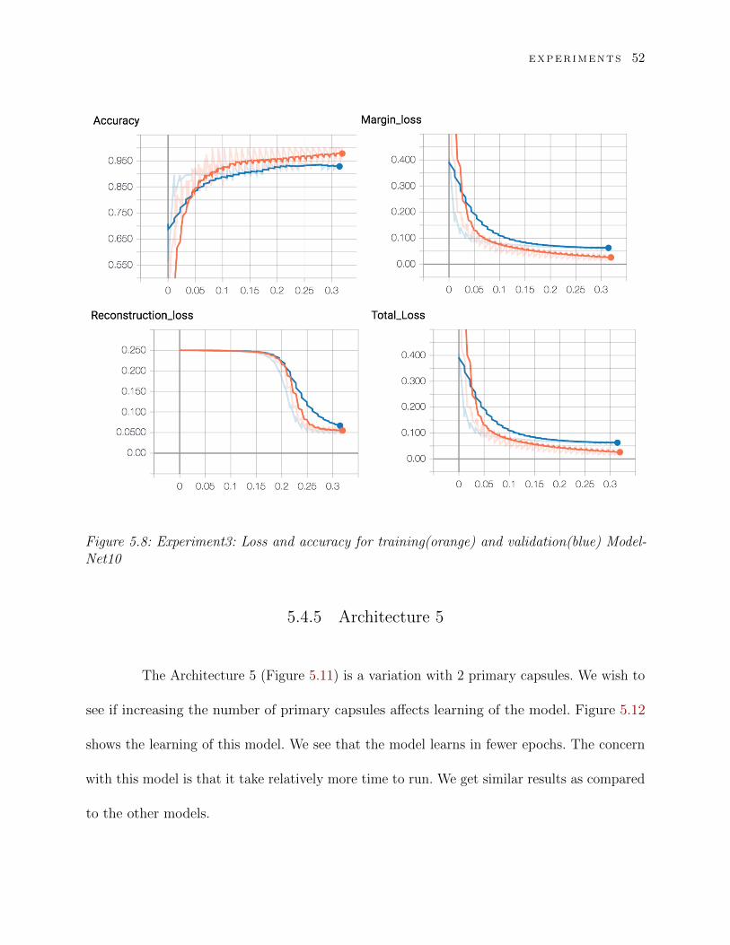
5.8 Experiment3: Loss and accuracy for training(orange) and validation(blue)
ModelNet10 . . . . . . . . . . . . . . . . . . . . . . . . . . . . . . . . . . . . 52
5.9 Architecture 4 . . . . . . . . . . . . . . . . . . . . . . . . . . . . . . . . . . . 53
5.10 Experiment4: Loss and accuracy for training (orange) and validation (blue)
ModelNet10 . . . . . . . . . . . . . . . . . . . . . . . . . . . . . . . . . . . . 54
5.11 Architecture 5 . . . . . . . . . . . . . . . . . . . . . . . . . . . . . . . . . . . 55
5.12 Experiment5: Loss and accuracy for training(orange) and validation(blue)
ModelNet10 . . . . . . . . . . . . . . . . . . . . . . . . . . . . . . . . . . . . 57
x

List of Tables
5.1 ModelNet10: Number of samples under each class . . . . . . . . . . . . . . . 42
5.2 ModelNet40: Number of samples under each class . . . . . . . . . . . . . . . 43
5.3 ShapeNet versus 3D CapsNet using 15% of data for training. . . . . . . . . . 46
5.4 ShapeNet versus 3D CapsNet using 5% of data for training. . . . . . . . . . 46
5.5 ShapeNet versus 3D CapsNet: Architecture-1 using 40% of data for training. 47
5.6 ShapeNet versus 3D CapsNet:Architecture 2 using 40% of data for training. 48
5.7 ShapeNet versus 3D CapsNet:Architecture 3 using 40% of data for training. 50
5.8 ShapeNet, 3D CapsNet:Architecture 4, 3D CapsNet:Architecture 2 using 40%
of data for training. . . . . . . . . . . . . . . . . . . . . . . . . . . . . . . . . 54
5.9 ShapeNet versus 3D CapsNet:Architecture-5 using 40% of data for training. 56
5.10 ShapeNet versus 3D CapsNet:Architecture-5 using 15% of data for training. 56
5.11 ShapeNet versus 3D CapsNet:Architecture-5 using 5% of data for training. . 56
5.12 Summary: Comparison of proposed architectures and ShapeNet(40% training
data) . . . . . . . . . . . . . . . . . . . . . . . . . . . . . . . . . . . . . . . . 56
5.13 Summary: Result of ShapeNet, Architecture 1 and Architecture 5 on different
split of dataset . . . . . . . . . . . . . . . . . . . . . . . . . . . . . . . . . . 58
5.14 Individual class accuracies (%) on ModelNet-10 with 40% training set. . . . . 59
xi

Chapter 1
Introduction
1.1 Motivation
Object recognition is a process for identifying an object in a digital image, 3D
space or video. Object recognition algorithms typically rely on matching, learning, or pattern
recognition algorithms using appearance-based or feature-based techniques. Object recognition
comprises a deeply rooted and ubiquitous component of modern intelligent systems. The
application of the technology related to 3D object recognition and analysis is increasing
day-by-day. Moreover, the effectiveness of 3D object recognition is increasing as researchers
are finding new algorithms, models and approaches and implementing them. The applications
for which 3D object recognition and analysis technology is used are:
1. Manufacturing Industry: 3D object recognition technology can make tasks like
manufacturing or maintenance more efficient in the aerospace, automotive and machine
industries. The advances in 3D object recognition technology is making robots more
1

INTRODUCTION 2
intelligent and autonomous as issues such as recognition of handing objects and obstacles
during navigation are being addressed.
2. Video surveillance : The usage of 3D object recognition technology in this area
includes tracking people and vehicles, segmenting moving crowds into individuals,
face analysis and recognition, detecting events and behaviours of interest and scene
understanding.
3. Medical and Health care: Deep learning and 3D object recognition is being widely
used in computer aided diagnosis systems in medical industry. Various applications
include analysis of 3D images from CT scans, digital microscopy and related fields.
4. Autonomous Driving: 3D object recognition is key to intelligent vehicles. For au-
tonomous driving, it is necessary to recognize and predict the motion of pedestrians,
other cars, bikes etc. Autonomous cars also need to recognize traffic signs, signals , road
area, sidewalks, guardrails, crosswalks, crossroads etc. In addition, understanding of
the scene by considering the context of the scene is required to predict future possible
dangers and prevent them. 3D object recognition technology can help accomplishing all
these goals.
5. Urban planning, Safety and Control: 3D object detection is widely used for damage
inspection, traffic monitoring, and rescue missions in urban areas. In addition, with the
help of drone technology, useful information related to urban planning can be acquired.
6. Augmented Reality - 3D: Object detection is a key component of an augmented
INTRODUCTION 3
reality system. Using 3D object technology in conjunction with augmented reality
systems can provide additional information and can be highly effective in fault diagnosis
and maintenance of industrial equipment.
Many of the existing 2D and 3D classification methods rely on convolutional neural
networks (CNNs), which are very successful in extracting features from the data. However,
CNNs cannot address the spatial relationship between features due to the max-pooling layers,
and they require vast amount of data for training.
The introduction of CapsNet by Dr. Hinton[1, 2] has intrigued many researchers to
understand how CapsNet works and apply it to their own research. CapsNet were developed
solely for 2D image classification. In this thesis, we are aiming to solve the problem of object
recognition from 3D volumetric data, and we propose a model architecture for 3D object
classification, which is an extension of Capsule Networks (CapsNets) to 3D data. Our proposed
architecture called 3D CapsNet, takes advantage of the fact that a CapsNet preserves the
orientation and spatial relationship of the extracted features, and thus requires less data to
train the network.
1.2 Problem Statement
Deficiency of data is a pronounced concern while training using a pure Convolutional
Neural Network(CNN)-based architecture. The problem becomes even more pronounced when
it comes to 3D data. There is a dearth of annotated datasets available for 3D data to train

INTRODUCTION 4
models, with even fewer training data. There has been several CNN-based approaches for
object classification and recognition from 3D data. However, CNN-based approaches require
larger datasets. The introduction of Capsule Network[1, 2] has opened doors to a new area of
research. Capsules have been used to recognize digits from MNIST dataset[3], and objects
from CIFAR[4] and Small NORB datasets[5]. These are 2D datasets with images. Capsules
have encoding for poses and orientations of the object i.e. neural activities are different for
same objects with different poses. Results of [2] show that Capsule Networks are better at
identifying multiple objects and also at generalizing among viewpoints than convolutional
neural networks. The motivation behind development of capsules is close depiction of neurons
arrangement in the brain. In this thesis, we propose a CapsNet architecture to solve the
problem of 3D object classification using Capsule Networks, extended for 3D data. Evaluation
of several architectures proves that CapsNet shows good promise, since the results obtained
with the proposed solution are better than a CNN-based approach even when we use less
training data.

OBJECT RECOGNIT ION BACKGROUND 5
Chapter 2
Object Recognition Background
2.1 Background and history
Contemporary computer vision study had its origins in the early 1960s [6]. Since then,
there have been many studies performed to correctly classify, recognize and detect objects in
images and 3D space. Some of the classical approaches include recognition using volumetric
parts [7, 8], geometric invariants [9–11], appearance-based recognition [12, 13], grammars
and related graphs representation [14, 15] and several others. More modern approaches,
such as scale invariant feature transform [16, 17], speeded up robust features [18], Principal
component analysis [19–21], linear discriminant analysis[22–24] and convolutional neural
networks[25–27], have been utilized to aid the process of recognizing objects. Convolutional
neural networks(CNNs) have allowed accomplishing the task of object recognition like never
before. CNNs have enabled object recognition in not only 2D images, but also in 3D models.
Numerous CNN models have been designed and have proven effective for this category of
tasks. Researchers have achieved state-of-the-art results by coalescing number of layers and

OBJECT RECOGNIT ION BACKGROUND 6
applying different mathematical functions to these layers.
Over the last several decades, researchers have been working towards object recogni-
tion using neural networks. Several algorithms and techniques have been developed, providing
state-of-the-art performance. The maturity of object recognition has helped its adoption in
large scale applications. Some of the notable works are the foundation to this thesis. In this
section, some of these notable works are mentioned and described in detail. The algorithms
mentioned in this section have not only been able to prove themselves in the academic research
domain, but also have been used in the production domain. Several companies have started
using 3D scanners to collect and generate 3D data from these scanners. The next steps to
data generation is always using data to extract knowledge from it. Object recognition is one
method to gather knowledge from 3D data.
2.2 Artificial Neural Networks
As the name suggests, artificial neural networks are logical networks mimicking the
functioning of the biological brain. Just like the brain, artificial neural networks are composed
of neurons connected to each other. Each artificial neuron is capable of transmitting signal
from the previous neuron to the subsequent one. Figure 2.1 shows a multilayer perceptron
with input layer, hidden layer and one output layer.
In an artificial neural network, the signal at an edge between artificial neurons is a
real number, and the output of each artificial neuron is gaged by a non-linear function of
the sum of its inputs. Artificial neurons and edges typically have a weight that updates as

OBJECT RECOGNIT ION BACKGROUND 7
Figure 2.1: An Artificial Neural Network
learning advances. The weight increases or decreases the strength of the signal at an edge.
Artificial neurons may have a threshold such that only if the aggregate signal crosses that
threshold is the signal sent. Artificial neurons are organized in layers. Different layers may
perform different kinds of transformations on their inputs. Signals travel from the first (input),
to the last (output) layer, possibly after traversing the layers multiple times.
2.3 Convolutional Neural Networks
The Convolutional Neural Networks (CNNs) are one of the most notable deep
learning approaches. A CNN is a class of deep, feed-forward networks, composed of one or
more convolutional layers with fully connected layers. It uses tied weights and pooling layers.
In general, a CNN is a hierarchical neural network, consisting of three main neural
layers: convolutional layers, pooling layers and fully connected layers. Figure 2.2 shows a
simple convolutional neural network.
OBJECT RECOGNIT ION BACKGROUND 8
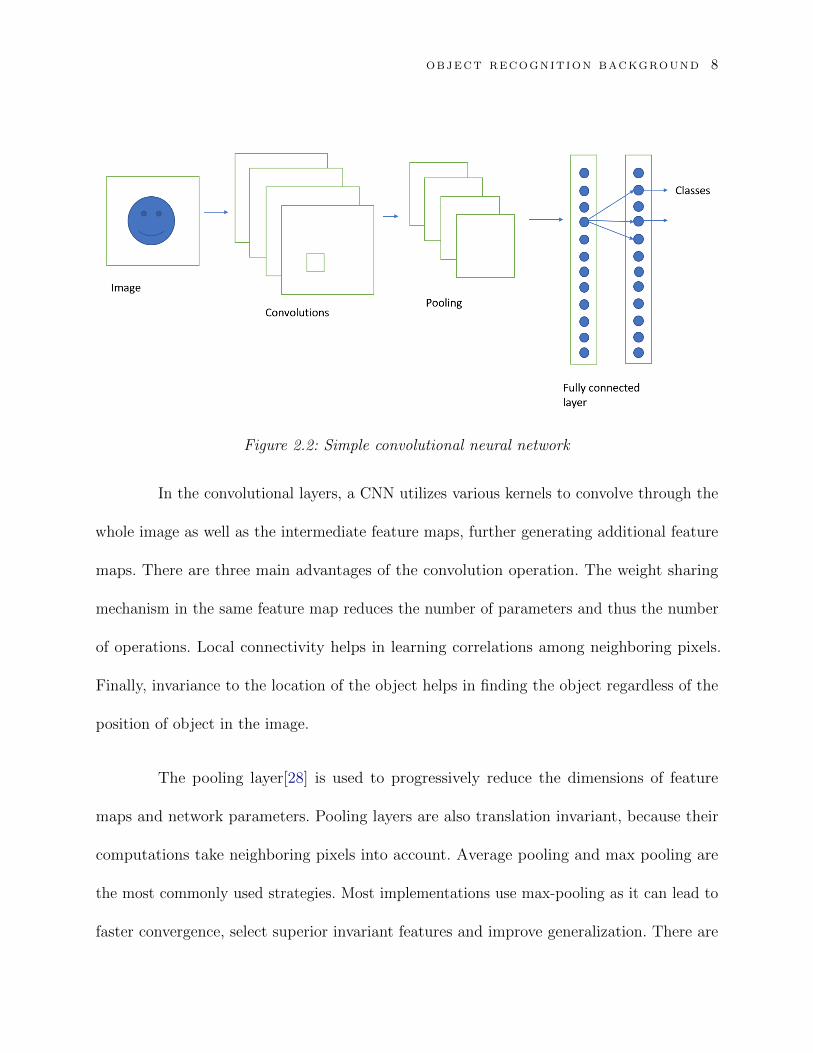
Figure 2.2: Simple convolutional neural network
In the convolutional layers, a CNN utilizes various kernels to convolve through the
whole image as well as the intermediate feature maps, further generating additional feature
maps. There are three main advantages of the convolution operation. The weight sharing
mechanism in the same feature map reduces the number of parameters and thus the number
of operations. Local connectivity helps in learning correlations among neighboring pixels.
Finally, invariance to the location of the object helps in finding the object regardless of the
position of object in the image.
The pooling layer[28] is used to progressively reduce the dimensions of feature
maps and network parameters. Pooling layers are also translation invariant, because their
computations take neighboring pixels into account. Average pooling and max pooling are
the most commonly used strategies. Most implementations use max-pooling as it can lead to
faster convergence, select superior invariant features and improve generalization. There are

OBJECT RECOGNIT ION BACKGROUND 9
three well-known approaches related to the pooling layers, each having different purposes.
Stochastic pooling[29] replaces the conventional deterministic pooling operations
with a stochastic procedure, by randomly picking the activation within each pooling region
according to a multinomial distribution. It is equivalent to standard max pooling but with
many copies of the input image, each having small local deformations. This stochastic nature
is helpful to prevent the overfitting problem. In Spatial Pyramid Pooling (SPP)[30] approach,
the last pooling layer of the CNN architecture is replaced with a spatial pyramid pooling
layer. The spatial pyramid pooling can extract fixed-length representations from arbitrary
images (or regions), generating a flexible solution for handling different scales, sizes, aspect
ratios. Max pooling and average pooling are useful in handling deformation, but they are not
able to learn the deformation constraint and geometric model of object parts. To deal with
deformation more efficiently, researchers introduced a new deformation constrained pooling
layer, called def-pooling layer, to enrich the deep model by learning the deformation of visual
patterns. It can substitute the traditional max-pooling layer at any information abstraction
level.
Fully-connected layers contain about 90% of the parameters in a CNN. Using this,
the neural network is fed forward into a vector with a pre-defined length. We could either
feed forward the vector into certain number of categories for image classification or take
it as a feature vector for follow-up processing. Though changing the structure of the fully-
connected layer is uncommon, some effort has gone in to make it more efficient. For example,
GoogLeNet[31] designed a deep and wide network by switching from fully connected to
sparsely connected architectures.

OBJECT RECOGNIT ION BACKGROUND 10
There are two stages for training the network - a forward stage and a backward stage.
First, the main goal of the forward stage is to represent the input image with the current
parameters (weights and bias) in each layer. Then the prediction output is used to compute
the loss cost with the ground truth labels. Second, based on the loss cost, the backward stage
computes the gradients of each parameter with chain rules. All the parameters are updated
based on the gradients and are prepared for the next forward computation. After sufficient
iterations of the forward and backward stages, the network learning can be stopped.
CNNs are usually trained by backpropagation (BP)[32] or Stochastic Gradient
Descent (SGD)[29] to find weights and biases that minimize certain loss function in order to
map the arbitrary inputs to the targeted outputs as closely as possible. BP algorithm refers
only to the method for computing the gradient, while SGD algorithm is used to perform
learning using this gradient. There are two key challenges in training CNNs: underfitting and
overfitting. Overfitting occurs when the gap between the training error and test error is too
large. Underfitting occurs when the model is not able to obtain a sufficiently low error on the
training set. In CNNs, there are two primary ways to combat overfitting: dropout and data
augmentation. Dropout is an inexpensive, powerful regularization strategy that can be seen
as a process of constructing new inputs by multiplication by noise. It is a method of adaptive
re-parametrization, motivated by the difficulty of training very deep neural network models.
Data augmentation is to artificially enlarge the dataset using label-preserving transformations.

OBJECT RECOGNIT ION BACKGROUND 11
2.4 3D data
3D data has three dimensions. It typically depicts real life objects and scenes. Most
3D can be shown in x, y and z coordinate space. 3D models can be constructed from data
collected from 3D scanners [33]. The first 3D scanners were introduced in the 1960s. 3D
technology has progressed since then. 3D data capture is the process of gathering information
from the real world, with x, y, and z coordinates, and making it digital. From there, it can
be processed in a number of ways to create any number of end products: 3D models, line
drawings, point clouds, fly through visualizations.
With the advent of several different types of 3D scanners, having state-of-the-art
specifications, it has become a challenge to be able to use the data collected from these 3D
scanners by first constructing 3D models and then recognizing objects in these models. Some of
the different types of 3D data are georeferenced and non-georeferenced [34, 35]. Georeferenced
data is one that describes a geographic location. It has longitude, latitude, and elevation as
the three different axes and center of the earth as the origin for these axes. Georeferenced
data can be collected by using satellite data and survey techniques. This data is collected by
starting at an identified point and then using relativity to construct the georeferenced data
for every point collected. Once the data is properly referenced, one georeferenced data can be
augmented with different georeferenced data and the combination can be used for numerous
applications requiring GPS and mapping applications. Non-georeferenced data is a type of
data which is collected without any identified known point. This kind of data can be used
for applications ranging from reverse engineering to crime scene detection to driverless cars

OBJECT RECOGNIT ION BACKGROUND 12
to drones. There are several methods of scanning 3D information, laser scanning, SONAR,
photogrammetry and structured light sensors are few to name.
Laser (or LiDAR)[36] scanning is one method that uses lasers to scan. A large
number of lasers are emitted from scanner and based on the surface these lasers are emitted
to, 3D data is generated by determining the location of 3D points. This generated data is
saved into a file known as point cloud. Pulsed based, airborne, phone-based, closed range are
few of the laser-based scanners.
Photogrammetry [37] is an old method that determines distances using photographs
to take measurements. In this method, massive number of photographs are uploaded to a
software that then perform numerous calculations on these photographs in order to create
point clouds. Since there are many assumptions and approximations used for this method, it
is not as accurate as laser scanning.
Structured light scanners[38] emit light on to surfaces and then use camera to and
software to measure how the light is distorted, which can then be used to create a point cloud
or model. Microsoft Kinect [39] is a famous structured light scanner. It uses projected dots of
infrared light and infrared camera to capture 3D data in real life.
Sonar[40] has typically been a method to use sound waves to find position in 2D
technology. However, in recent times, sonar has been extended to construct point clouds of
underwater environments.
Another important primitive type of 3D data is data from CAD models [41]. Software

OBJECT RECOGNIT ION BACKGROUND 13
Figure 2.3: Different viewpoints of a 3D object
is used to create these models in 3D spaces. In this thesis, CAD model’s dataset is used
for the experimental results. However, these algorithms are capable of being extended to
use on point clouds as well. CAD is an important step in the development process of many
industrial applications involving mechanical parts. 3D CAD has several benefits since it
allows visualization and optimization of designs, avoids unnecessary costs due to human error,
and provides reproducibility of the experiments under various conditions such as different
viewpoints, different sizes etc. Figure 2.3 shows one 3D object viewed from different angles.
2.5 Contemporary related work
Advancements in 3D data collection technologies induced research for many appli-
cation areas. This has led to the proposal of different methods for object classification. In
this section, we discuss some of the related works in the domain of object classification using
neural networks.
OBJECT RECOGNIT ION BACKGROUND 14
[42] discusses an approach for using 3D CNNs which they call C3D. Spatio-temporal
features are those that contain information about the space and time, e.g. moving objects
that can exist in space in a given time. They prove that 3D CNNs are more suitable for
spatiotemporal feature learning compared to 2D CNNs. The architecture they use is a
homogeneous one with small 3× 3× 3 convolution kernels in all layers and this architecture is
the best among the different architectures for 3D ConvNets (best temporal kernel length for
3D ConvNets). Inspired by this work, we are using 3D convolutions in the convolution layers.
3D ShapeNets[26] learns the distribution of complex 3D shapes across diverse object
classes and arbitrary poses. A deep belief network is proposed with convolutions to realize the
complex joint distribution of 3D objects which are converted to voxels. They have extended
the deep belief network for 2D data to 3D data by first reducing the size of feature map using
few convolution layers and then using fully connected layers. By creating this network, they
have been able to recognize objects and also reconstruct 2.5D objects from RGBD sensors. In
addition to the belief network, they also contribute to the 3D data community by publishing
their dataset, ModelNet, which they also use to train their network. ModelNet dataset is a
3D CAD model dataset which is used in our work as well. Figure 2.4 shows the architecture
of the ShapeNet deep belief network.
[27] is another important model in the research of object recognition in 3D data.
It uses 3D CNN architecture. In their approach, the point cloud inputs are converted to
occupancy grids of size 32× 32× 32. These occupancy grids symbolize the state of the object
and its surroundings as a 3D mesh of random variables (each corresponding to a voxel) and
preserve a probabilistic approximation of their occupancy as a function of inward sensor

OBJECT RECOGNIT ION BACKGROUND 15
Figure 2.4: ShapeNet architecture
data and prior knowledge. Two convolution layers are applied to the occupancy grid creating
smaller feature maps. Pooling is applied to the output of the second convolutional layer. This
is followed by a fully connected layer of 128 neurons and this is connected to the output
layer which is equivalent to the number of classes in the dataset. This model first achieves
volumetric representation in the form of occupancy grids as 3D mesh of random variable. This
allows to proficiently evaluate free, occupied and unknown area from range measurements,
even for measurements coming from different viewpoints and time instants. They can be
stored and manipulated with simple and efficient data structures such as matrices. This is a
novel approach because most framework uses 0s and 1s to describe 3D data. They are also
able to achieve good classification results by using the 3D CNN architecture.
By assembling several layers, the network can construct a hierarchy of more com-
pound features representing larger regions of space, leading to a global label for the input
occupancy grid. Finally, hypothesis is merely feed-forward and can be performed efficiently
with commodity graphics hardware.

OBJECT RECOGNIT ION BACKGROUND 16
Another approach has been applied by [43] which represents 3D data using view-
based descriptors. The shape of the 3D object is described by compilation of 2D projections
of the objects. This can be visualized as using a camera to click several pictures going around
the object and creating a collection. The authors of [43] describe the reason for developing a
multi-view algorithm as opposed to using 3D shape. First, the size of organized databases with
annotated 3D models is rather limited compared to image datasets. For example, ModelNet
contains 127,915 CAD Models. Whereas, the ImageNet database contains several millions of
annotated images. Second, 3D shape descriptors tend to be very high-dimensional, making
classifiers prone to overfitting. On the other hand, view-based descriptors have a number of
desirable properties: they are relatively low-dimensional, efficient to evaluate, and robust to
3D shape representation artifacts, such as holes, imperfect polygon mesh tessellations and
noisy surfaces. The rendered shape views can also be directly compared with other 2D images,
silhouettes or even hand-drawn sketches. In [43], multiple views are aggregated in order
to amalgamate the information from all views into a single, compact 3D shape descriptor.
Multi-view CNN offers better results and more efficient retrieval performance during retrieval
compared to methods which are based on pairwise comparisons of image descriptors. In
this thesis, we use a relatively small amount of data to show that training can in fact, be
done with a smaller dataset as well. We do not need several millions of annotated shapes to
effectively train a 3DCapsNet classifier.
Residual neural networks have been demonstrated to be easier to optimize and do not
suffer from vanishing/exploding gradients observed in deep networks. In [44] a residual neural
network has been implemented for 3D object classification of the 3D Princeton ModelNet
OBJECT RECOGNIT ION BACKGROUND 17
dataset. It has also been shown that widening network layers dramatically improves accuracy
in shallow residual nets and improves classification accuracy.
They present their results with developing volumetric CNN architectures that utilize
wide residual layers on classification on the ModelNet-40 dataset. A widening factor has been
defined, where the factor multiplies the number of features in convolutional layers. This was
used to evaluate the effect of further widening of the residual layers on classification accuracy.
To enhance their dataset, the training samples were augmented by randomly rotating each
3D shape along a randomly designated axis to increase variance and the model’s capability to
generalize. The model was trained with batch sizes of 64 and during training, weights were
saved every epoch for 10 epochs and a final model consisting of an ensemble of weights from
each epoch was used.
While this approach gets state-of-the-art results, it is important to remember
the magnum model parameters and computation time. Thus, we aim to build a shallow
architecture to be able to build on simpler hardware, requiring lesser computation power.

Chapter 3
Capsules
A capsule is a group of neurons that together perform internal computations on
inputs given to them and encapsulate the output into a small vector which is capable of
representing different properties of the same entity . In [1], Hinton talks about the deficiencies
of previously existing methods of object recognition such as CNN and Scale Invariant feature
transform (SIFT).
In a CNN, there are a number of layers of learned feature detectors that gives a
scalar output. These networks aim for viewpoint invariance by using max-pool to abridge
the activities of duplicated feature. What max-pool essentially does is the following: it finds
components in an object and based on that affirms that the object is present. However,
spatial relationships of the parts are not relevant to the CNN, thus making them invariant to
features but not equivariant. Equivariance is detection of objects that can transform to each
other. For instance, if an object is rotated at an angle, then by the property of equivariance,
capsules can recognize that the object is rotated at that angle, without necessitating training
18

CAPSULES 19
with that variation of image. This is a unique quality of capsules over its predecessor, CNNs,
which required training with all variation of the object such as orientation, pixel intensities,
scale etc.
Scale Invariant Feature Transform[16] combines the unambiguous representations
of pose of the features of the objects and offers vector as output. These feature vectors are
invariant to scale, rotation, illumination, and translation. However, scale invariant feature
transform is a complicated technique and is typically hand-crafted.
Capsules have two primary constituents. One is the locally invariant probability
that an entity is present. Second is the set of the instantiation parameters, also known as
pose, that are equivariant. It is important to have these two constituents because they help
in recognizing the whole object by recognizing their parts.
With this concept in mind Hinton published three research papers [1, 2, 45], which
opened up door to a new field of research and are also the foundation of this thesis.
3.1 Transforming Auto-Encoders
In [1], transforming auto-encoders has been proven to be able to easily learn
from pairs of transformed images provided that there is a straightforward approach to the
transformations. Auto-encoders are simple neural networks with 3 layers. One important
application for this is data compression and retrieval. Figure 3.1 shows the simplest auto-
encoder. Complexity can be defined with the encoder and decoder unit.

CAPSULES 20
Figure 3.1: Simple Auto-encoder
The transforming auto-encoders are described as having both recognition and
generation units.
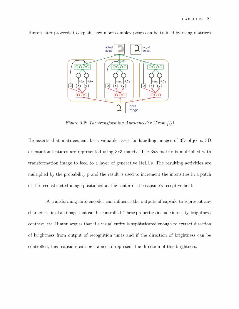
[1] describes a simple transforming encoder which has three capsules, each capsule
has three recognition units and four generation units. It receives an image and shift variables
∆x and ∆y as input, uses the recognition unit to read image and perform computations on
the image to give out x, y, and p as output, where x and y are pose information and p is
the probability that an entity is present in the image. The generation units then use the
pose information x, y summed up with ∆x and ∆y, respectively, to compute an intermediate
output, which when multiplied with the p gives the output image. By back-propagating on the
mutation between the original and transformed image, the weights are learned. The capsules
work independently until the final layer where they collaborate to create the output image.
Figure 3.2 shows three capsules of a transforming auto-encoder that models translations.
CAPSULES 21
Hinton later proceeds to explain how more complex poses can be trained by using matrices.
Figure 3.2: The transforming Auto-encoder (From [1])
He asserts that matrices can be a valuable asset for handling images of 3D objects. 3D
orientation features are represented using 3x3 matrix. The 3x3 matrix is multiplied with
transformation image to feed to a layer of generative ReLUs. The resulting activities are
multiplied by the probability p and the result is used to increment the intensities in a patch
of the reconstructed image positioned at the center of the capsule’s receptive field.
A transforming auto-encoder can influence the outputs of capsule to represent any
characteristic of an image that can be controlled. These properties include intensity, brightness,
contrast, etc. Hinton argues that if a visual entity is sophisticated enough to extract direction
of brightness from output of recognition units and if the direction of brightness can be
controlled, then capsules can be trained to represent the direction of this brightness.

CAPSULES 22
3.2 Matrix Capsules with EM Routing
In [45], the capsule constitutes an activation and a pose. An activation is a logistic
unit to signify the presence of an entity and pose is a 4 x 4 matrix to signify relationship
between an entity and the observer. Basis of CNN is that the visual detector demands usage
of the same knowledge at all locations in the image. This is attained by binding weights
of detected features learned at one position to others. The authors argue that view point
changes such as azimuth, elevation etc. have a complex impact on pixel intensities but simple,
linear effect on pose matrix. Capsules aim high dimensional coincidence filtering by utilizing
the underlying linearity. They use it to both, deal with variations in view point as well as
improve segmentation decisions. High dimension coincidence filtering is the property which
helps to detect a familiar object by looking for an agreement between votes for its pose
matrix. These votes are derived from parts previously detected. EM routing algorithm is
performed on both activation and the votes matrix. EM algorithm is classically used for
fitting a mixture of Gaussians [46]. After a number of iterations of EM routing, tight clusters
of high dimensional votes are formed. Loose particles of irrelevant votes are also formed.
A capsule network can be visualized by imagining layers of several capsules arranged
sequentially. ΩL denotes all the capsules in layer L. Values of components in a capsule, i.e.
activation probability a and pose matrix M, are not stored since they depend on the current
input. The weights are the only stored parameters and are learned discriminatively. The
weights are a 4x4 transformation matrix which are trained over several epochs. The weight
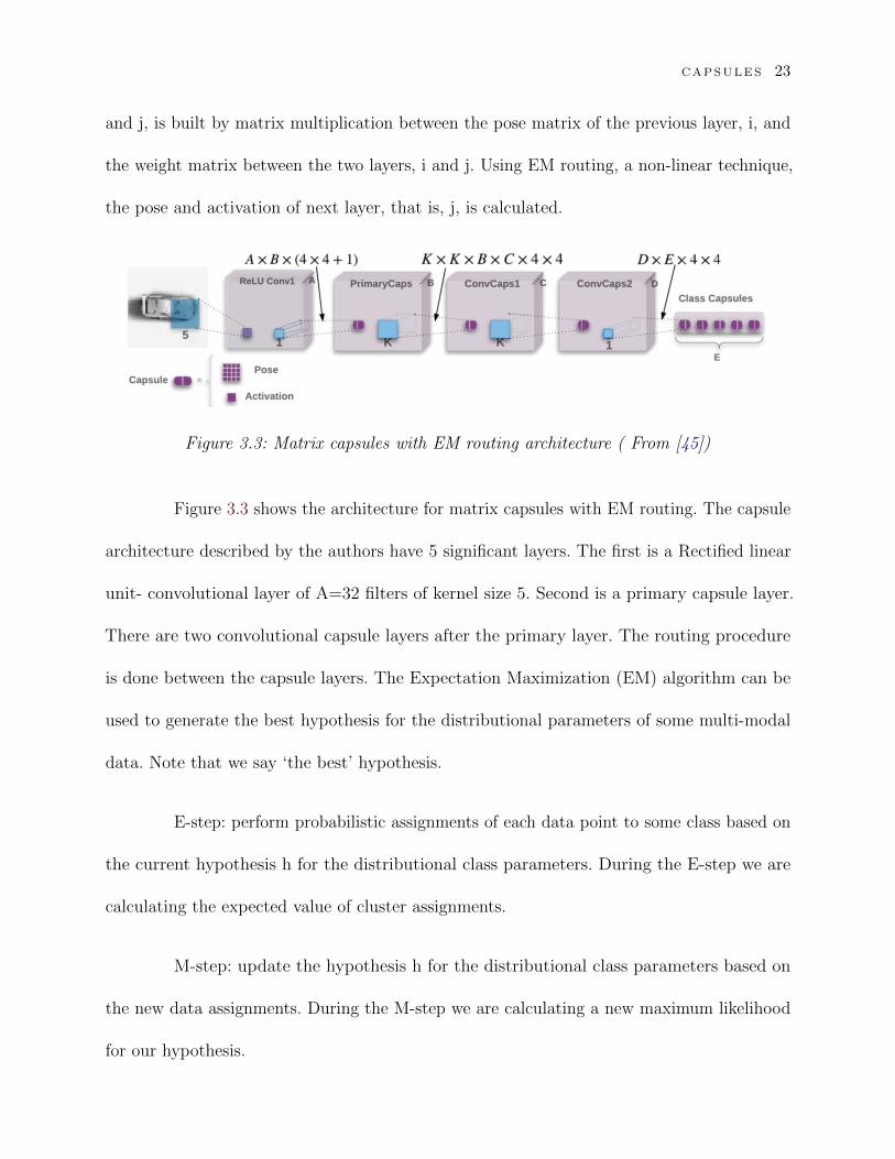
matrices are designed to exist between the capsule layers. The vote matrix for two layers, i
CAPSULES 23
and j, is built by matrix multiplication between the pose matrix of the previous layer, i, and
the weight matrix between the two layers, i and j. Using EM routing, a non-linear technique,
the pose and activation of next layer, that is, j, is calculated.
Figure 3.3: Matrix capsules with EM routing architecture ( From [45])
Figure 3.3 shows the architecture for matrix capsules with EM routing. The capsule
architecture described by the authors have 5 significant layers. The first is a Rectified linear
unit- convolutional layer of A=32 filters of kernel size 5. Second is a primary capsule layer.
There are two convolutional capsule layers after the primary layer. The routing procedure
is done between the capsule layers. The Expectation Maximization (EM) algorithm can be
used to generate the best hypothesis for the distributional parameters of some multi-modal
data. Note that we say ‘the best’ hypothesis.
E-step: perform probabilistic assignments of each data point to some class based on
the current hypothesis h for the distributional class parameters. During the E-step we are
calculating the expected value of cluster assignments.
M-step: update the hypothesis h for the distributional class parameters based on
the new data assignments. During the M-step we are calculating a new maximum likelihood
for our hypothesis.

CAPSULES 24
In this capsule architecture, spread loss is used to desensitize the training to unique
hyper-parameters. This is done in order to maximize the activation is of target class and the
activation of other classes.
3.3 Dynamic Routing Between Capsules
In [2], CapsNet is based on multiple layers of capsules where capsules from one layer
make predictions for capsules at a higher level. The higher-level capsule becomes active when
different expectations harmonize. This is known as routing by agreement. This process is
implemented for several iterations. [2] prove that this method is more effective compared to
the max pooling method which chooses the most prominent feature amongst a set of features
and disregards the other features. By doing this, it is able to achieve invariance. However, the
goal of CapsNet is not to achieve invariance, but equivariance. Equivariance helps the model
recognize an object even if the pose of the object is different from objects the model has
learned before. It also helps remember the spatial relationship of the features of the objects.
In order to achieve equivariance, scalar features are substituted by vector features and pooling
is swapped by routing by agreement. Figure 3.4 shows the architecture for dynamic routing.
Figure 3.4: Dynamic Routing between capsules(From [2])
CAPSULES 25
Squashing is a non-linear function applied to the output vector to ensure that vectors
which have low probability are minimized to near zero leaving the high probability vectors to
be near one. Discriminative learning which learns the probability y given x, helps to use the
output of squashing.
Routing by agreement is done by using dynamic routing. An initial weight vector
is created and is multiplied by the output of the capsules of the lower levels, creating the
prediction vector u, after which all these prediction vectors are summed up in a weighted
manner, creating an input to the higher-level capsule. The output of current capsule is
represented as v and the agreement between the layers is calculated by a scalar product
between output of current capsule v and prediction of the lower capsule u.
There are two kinds of losses that are used. Margin loss is the loss that pronounces
the existence of a particular class. If the class is present in the image, then the vectors have a
higher value. Reconstruction loss is another type of loss to encode the instantiation parameter
of the input class. A mask is created for the activity vector of the correct class and this is
used to reconstruct the output of the digit (class) capsule, both of which are fed into the
decoder. By doing this, they use reconstruction loss as a regulator. The total loss is sum of
the two losses, reconstruction loss being factored down by a value of 0.0005.
The aforementioned capsule model is a key building block in this proposed research.
We use this capsule model as the base to build our 3D version of the Capsule Net model.
Chapter 4
3D CapsNet
As mentioned before, CNNs have several deficiencies. Firstly, CNNs do not check
the relative positions of features with respect to each other. Secondly, they need a large
amount of data to generalize the classifier. Thirdly, it is believed that CNNs are not a good
representation of the human vision system. In a CNN, all low-level details are sent to all
the higher-level neurons. These neurons then perform further convolutions to check whether
certain features are present. This is done by striding the receptive field and then replicating
the knowledge across all the different neurons. Capsule network (CapsNet) tries to overcome
these shortcomings of CNNs.
Main features of CapsNets are that neurons (which output scalar values) are replaced
with capsules (which output vectors). A capsule contains several neurons, and together they
represent instantiation parameters of a feature. Like neurons, capsules are also stacked into
layers. However, unlike convolutional layers, capsule layers activate only certain capsules
that best represent the incoming image (or just a feature). A CapsNet solves the issues
26

3D CAPSNET 27
of CNNs by treating different orientations of an image as the same object. Hence, less
training examples suffice during the training of CapsNets. The CapsNet solves the issue of
translational invariance by preserving the geometric dependence of features. If a chair and
bed both have four legs, a CNN may confuse the two objects. However, a CapsNet preserves
the orientation and relationship of those features and results in correctly classifying the two
objects. The introduction of CapsNets has begun to stimulate additional wave of research,
that will hopefully lead to development of very useful and powerful applications.
In this work, we propose a novel method of classifying 3D objects from 3D volumetric
data. We experiment with different variations of the method. We thus propose a vector capsule
network model with dynamic routing for 3D volumetric data.
4.1 The key components of 3D CapsNet
4.1.1 3D Convolutions
The Convolution layer detects the basic features in the 3D data to create activities
for these features. 3D convolutions involve filters of 3 dimensions (x, y and z) and thus are
also known as spatial convolutions. This filter is moved in the three dimensions producing
3D output.

3D CAPSNET 28
Figure 4.1: 3D convolutions
4.1.2 Primary Capsule
Primary capsule helps in implementing Hinton’s view of inverse graphics. Hierarchy
of parts is a concept used which explains that a higher level visual entity is present if several
lower level visual entities can agree on their predictions for its pose. In the concept of capsules,
lower level capsule helps the higher level predict if an entity is present. Primary capsules are
thus bottommost level of multi-dimensional objects.
4.1.3 Squash Function
The squash function is applied to output of capsule to shorten the length of capsule
vectors. It is a non-linearity function just like ReLU, Sigmoid, etc. However, unlike ReLU,
which work well with scalars, squash function has proven to work better with capsules.
The above function squashes to 0 if the output is a short vector and tries to constrain
the output vector to 1 if the vector is long. According to [2], the squash function is defined

3D CAPSNET 29
as follows:
vj =||sj||2
1 + ||sj||2sj||sj||
(4.1)
4.1.4 Class Capsule
Class capsule has 16D output per object class. Dynamic routing algorithm is
employed between the primary and class capsule layers. The routing algorithm is used to
achieve an agreement between the primary and class capsule layers. Essentially, the lower
level capsule sends its input to higher level to receive an agreement. A non-linear squash
function is used within the routing algorithm in order to change the length of vector to less
than one, yet preserving the direction of the vector, thereby representing the weights as
probabilities with direction.
4.1.5 Routing Algorithm
A routing algorithm is used to resolve which capsule gets activated for the incoming
data. Dynamic routing is a very important networking technique that helps select path
according to the real-time layout changes. Dynamic routing algorithm is employed between
the primary and class capsule layers and is used to achieve an agreement between the primary
and class capsule layers. Dynamic routing helps to strengthen prediction value by using an
agreement protocol. The lower level capsule sends its input to the higher level, which agrees
with its input. Weight matrices are updated using this agreement between the two levels
of capsules. The routing algorithm performs a similar function as the max pooling layer.

3D CAPSNET 30
However, while the max pooling layer chooses the most prominent features eliminating the
non-prominent ones, the routing algorithm does not eliminate the features, but routes to the
right feature instead.
The number of iterations for routing is a hyper parameter and has been chosen, as
per [2] as 3, since larger values of routing iteration lead to more overfitting.
4.1.6 Reconstruction Loss
Reconstruction loss is used as regularization to learn a global linear manifold between
a whole object and the pose of the object as a matrix of weights via unsupervised learning.
As such, the translation invariance is encapsulated in the matrix of weights, and not in the
neural activity, making the neural network translation equivariant.
4.1.7 Decoder
The decoder takes the output of the class capsules and reconstructs the object from
it. There are three fully connected layers in our model’s decoder. The first two fully connected
layers use activation as ReLU and the last one uses Sigmoid activation.
3D CAPSNET 31
4.2 Optimizations
4.2.1 Leaky ReLU
The Rectified Linear Unit (ReLU) is an activation function that computes the
function f(x)=max(0, x) In other words, the activation is simply thresholded at zero. However,
this leads to neuron values to become zero. Sometimes this may happen at early stages of
training. It is not desirable as sometimes this may cause the neurons to never get activated
on any input. Leaky ReLUs are one attempt to fix the “dying ReLU” problem. Instead of
the function being zero when x < 0, a leaky ReLU will instead have a small negative slope
(of 0.01, or so). That is, the function computes
f(x) = (x < 0)(αx) + (x >= 0)(x)f(x) = 1(x < 0)(αx) + 1(x >= 0)(x) (4.2)
where α is a small constant.
4.2.2 Batch Normalization
It is the process of normalizing the data in the mini-batch. Batch Normalization
allows us to use much higher learning rates and be less careful about initialization. It helps
the layers learn more independently of other layers. It helps reduce overfitting by small
factor. Used together with dropout helps in reducing overfitting better. It helps improve the
stability of a neural network by normalizing the output of the previous activation layers.

3D CAPSNET 32
This normalization is done by subtracting the batch mean and dividing the same by batch
standard deviation.
4.2.3 Dropout
Dropout is a regularization procedure for reducing overfitting in neural networks by
averting complex co-adaptations on training data. It is a very efficient way of performing
model averaging with neural networks. The term “dropout” refers to dropping out units
(both hidden and visible) in a neural network. We can specify the percentage of neurons to
drop in the function.
4.3 Data Preprocessing
ModelNet10 and ModelNet40 datasets have been used to train and test our model.
These datasets are available in “.off” format. To be able to train and test the model, we are
required to convert the dataset into a format that is understood by tensors. We decided to
use process of Voxelization to convert the datasets from “.off” to voxels. The voxels are saved
in “.npz” format to be able to use in our experiments.
Voxelization converts 3D objects into a number of voxels or occupancy grids of fixed
size using clipping and sampling of 3D objects. Binary voxel grid used has merely two states.
They are occupied state and unoccupied state. Voxelization fits diverse sized 3D objects into
fixed size consistent grids without the loss of the spatial information of the objects. Both

3D CAPSNET 33
Figure 4.2: 3D Binary Voxels
Modelnet10 and ModelNet40 are converted to 3D Numpy arrays of 30× 30× 30.
4.4 3D CapsNet Architecture
4.4.1 Architecture 1
Our first proposed model has a shallow architecture with two 3D convolution layers,
a 3D max pooling layer, followed by the primary and class capsule layers. Between the
convolution layers and the max pooling layer, batch normalization is performed. The conv1
layer has 48-many 5 × 5 × 5 filters with stride 1. The conv2 has 96-many 5 × 5 × 5 filters
with stride 1. These layers convert pixel intensities to local features. The pooling layer is
used to reduce the overfitting by reducing the dimensionality of the feature maps. The batch
normalization process is used to speed up the training process of the classifier by addressing
the problem of internal covariate shift, thus allowing us to use higher learning rate for more
iterations. Primary capsule layer that follows the max-pooling layer contains a convolutional
3D CAPSNET 34
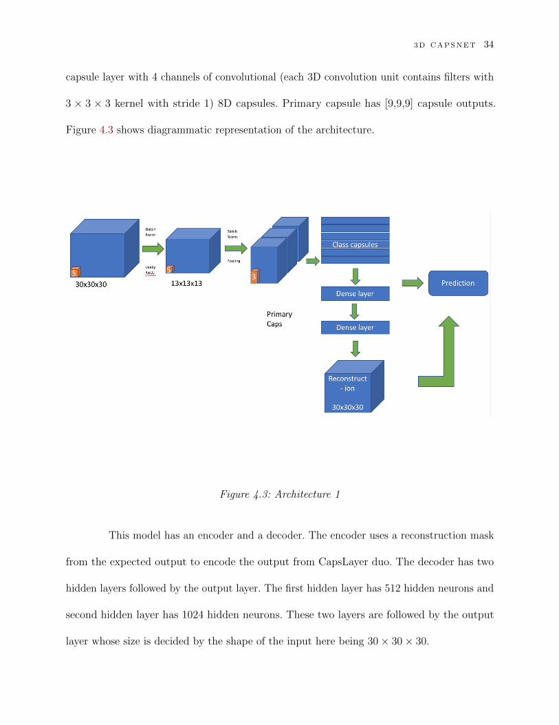
capsule layer with 4 channels of convolutional (each 3D convolution unit contains filters with
3 × 3 × 3 kernel with stride 1) 8D capsules. Primary capsule has [9,9,9] capsule outputs.
Figure 4.3 shows diagrammatic representation of the architecture.
Figure 4.3: Architecture 1
This model has an encoder and a decoder. The encoder uses a reconstruction mask
from the expected output to encode the output from CapsLayer duo. The decoder has two
hidden layers followed by the output layer. The first hidden layer has 512 hidden neurons and
second hidden layer has 1024 hidden neurons. These two layers are followed by the output
layer whose size is decided by the shape of the input here being 30× 30× 30.

3D CAPSNET 35
4.4.2 Architecture 2
In our second model, we use one 3D convolution layer, followed by the primary and
class capsule layers. Batch normalization is used after the convolution layer and before the
primary capsule layer. The conv1 layer has 64-many 5 × 5 × 5 filters with stride 2. These
layers convert pixel intensities to local features. Leaky ReLU is used to improve the activation.
The batch normalization process is used to speed up the training process of the classifier by
addressing the problem of internal covariate shift, thus allowing us to use higher learning rate
for more iterations. Dropout is used between convolution layer and primary capsule layer
with probability of keeping as 0.5. The primary capsule layer that follows the max-pooling
layer contains a convolutional capsule layer with 4 channels of convolutional 8D capsules.
Each 3D convolution unit contains filters with 5× 5× 5 kernel with stride 1. The stride is
kept at 1 to prevent further loss of information using higher value of strides. Primary capsule
for ModelNet has [9,9,9] capsule outputs. Figure 4.4 shows diagrammatic representation of
the architecture.
The number of class capsules are 10 for ModelNet10 and 40 for ModelNet40. This
model has an encoder and a decoder. The encoder uses a reconstruction mask from the
expected output to encode the output from CapsLayer duo. The decoder has two hidden
layers followed by the output layer. The first hidden layer has 512 hidden neurons and second
hidden layer has 1024 hidden neurons. Another dropout layer is used in the decoder unit.
Leaky ReLU is used with both hidden layers and the dropout is used after the second one.
These two layers are followed by the output layer whose size is decided by the shape of the

3D CAPSNET 36
Figure 4.4: Architecture 2
input here being 30× 30× 30.
4.4.3 Architecture 3
In our third model, we use two 3D convolution layer, followed by the primary and
class capsule layers. The conv1 layer has 48-many 5× 5× 5 filters with stride 2. The conv2
has 96-many 5 × 5 × 5 filters with stride 1. These layers convert pixel intensities to local
features. Batch normalization is used after the convolution layer and before the primary
capsule layer. Leaky ReLU is used to improve the activation. The batch normalization process
3D CAPSNET 37
is used to speed up the training process of the classifier by addressing the problem of internal
covariate shift, thus allowing us to use higher learning rate for more iterations. Dropout
is used between convolution layer and primary capsule layer with probability of keeping
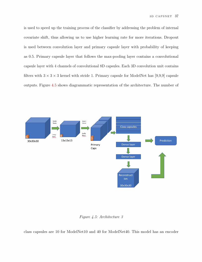
as 0.5. Primary capsule layer that follows the max-pooling layer contains a convolutional
capsule layer with 4 channels of convolutional 8D capsules. Each 3D convolution unit contains
filters with 3× 3× 3 kernel with stride 1. Primary capsule for ModelNet has [9,9,9] capsule
outputs. Figure 4.5 shows diagrammatic representation of the architecture. The number of
Figure 4.5: Architecture 3
class capsules are 10 for ModelNet10 and 40 for ModelNet40. This model has an encoder

3D CAPSNET 38
and a decoder. The encoder uses a reconstruction mask from the expected output to encode
the output from CapsLayer duo. The decoder has two hidden layers followed by the output
layer. The first hidden layer has 512 hidden neurons and second hidden layer has 1024 hidden
neurons. Another dropout layer is used in the decoder unit. These two layers are followed by
the output layer whose size is decided by the shape of the input here being 30× 30× 30.
4.4.4 Architecture 4
Our next model has only one convolutional layer. This convolution layer has 64
kernels of size 5 and stride 2 and activation as leaky ReLU. We use batch normalization
and dropout of 0.4. The convolutional layer is followed by primary convolutional layer. The
primary capsule has convolution units of size 5 and stride 1. This is followed by class capsule
layer. The number of class capsules are 10 for ModelNet-10 and 40 for ModelNet-40. Figure 4.6
The decoder here has only one hidden layer with 512 neurons. We use leaky ReLU activation
with this hidden layer. This is followed by a dropout layer, followed by the output layer.
These two layers are followed by the output layer whose size is decided by the shape of the
input here being 30× 30× 30.
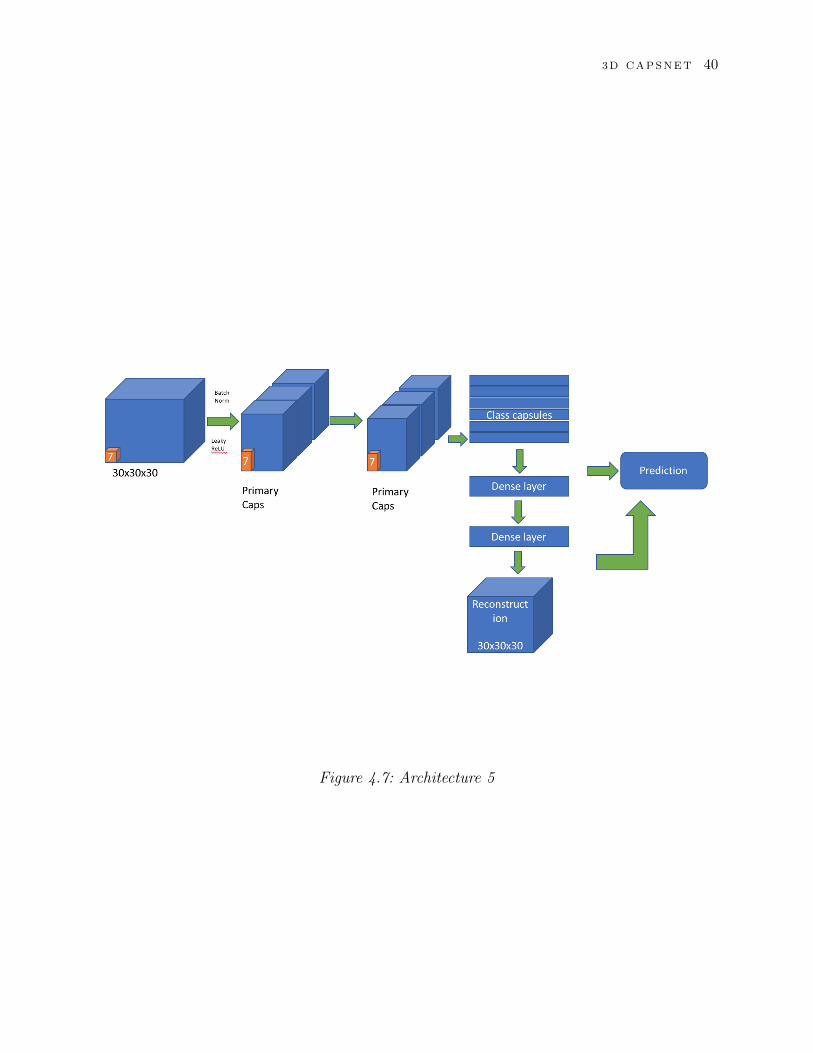
4.4.5 Architecture 5
Our final architecture has two primary capsule layers. The first layer is a convolutional
layer with 64 filters of kernel size 7 and stride 1. Activation used is leaky ReLU. Dropout
with probability to keep = 0.4 is used after the convolutional layer. Just as the previous
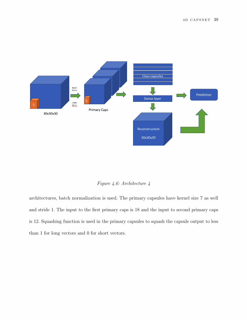
3D CAPSNET 39
Figure 4.6: Architecture 4
architectures, batch normalization is used. The primary capsules have kernel size 7 as well
and stride 1. The input to the first primary caps is 18 and the input to second primary caps
is 12. Squashing function is used in the primary capsules to squash the capsule output to less
than 1 for long vectors and 0 for short vectors.
3D CAPSNET 40
Figure 4.7: Architecture 5

EXPERIMENTS 41
Chapter 5
Experiments
5.1 ModelNet Dataset
Figure 5.1: ModelNet10 Mesh
Princeton ModelNet project [47] provides a comprehensive clean collection of 3D
CAD models of objects covering most common object categories. In this work, we have
used the 40-class subset as well as the 10-class subset of the full dataset. The classes in the
modelnet10 dataset are bathtub, bed, chair, desk, dresser, monitor, nightstand, sofa, table,
and toilet. The number of objects in each class are shown in the figure below. 5.1 displays
the different categories under ModelNet10 viewed using the software Meshlab. Number of

EXPERIMENTS 42
Table 5.1: ModelNet10: Number of samples under each class
Bathtub Bed Chair Desk Dresser156 615 989 286 286
Monitor NightStand Sofa Table Toilet565 286 780 490 444
samples per category are mentioned in the table 5.1.
The modelnet40 dataset has objects from 40 classes. The number of samples per
class are shown in the table 5.2. These datasets are available in “.off” format. Object File
Format (.off) files are used to represent the geometry of a model by specifying the polygons
of the model’s surface. The polygons can have any number of vertices.
The .off files in the Princeton Shape Benchmark conform to the following standards:
OFF files are all ASCII files beginning with the keyword OFF. The next line states the
number of vertices, the number of faces, and the number of edges. The number of edges can
be safely ignored. The vertices are listed with x, y and z coordinates, written one per line.
After the list of vertices, the faces are listed, with one face per line. Voxelization is used to
convert OFF into binary voxels and voxels are converted to numpy format that can be used
in our algorithms.

EXPERIMENTS 43
Table 5.2: ModelNet40: Number of samples under each class
Airplane Bathtub Bed Bench Book shelf Bottle Bowl Car8712 1872 7380 2316 8064 5220 1008 3564Chair Cone Curtain Cup Desk Door Dresser Flower Pot11868 2244 1188 1896 3432 1548 3432 2028
Glass Box Guitar Keyboard Lamp Laptop Mantel Monitor Person3252 3060 1980 1728 2028 4608 6780 3432
Night Stand Piano Plant Radio Range hood Sink Sofa Stairs1296 3972 4080 1488 2580 1776 9360 1728Table Stool Tent Toilet TV Stand Vase Wardrobe Xbox1320 5904 2196 5328 4404 6900 1284 1476
5.2 Hardware
The Alienware system in Smart Vision Lab has been used to implement the 3D
CapsNet and to run all the experiment. It has the following configurations:
Architecture: x86 64
CPU op-mode(s): 32-bit, 64-bit
Byte Order: Little Endian
CPU(s): 8
Model name: Intel(R) Core(TM) i7-7700K CPU @ 4.20GHz
The GPU configurations are as in fig. 5.2:
5.3 Software
Software and libraries used for this research are as below:

EXPERIMENTS 44
Figure 5.2: GPU config
Python 3.5
Tensorflow 1.3
Numpy
Scikit-learn
MeshLab
5.4 Experiments on proposed architectures
In this section we present the results of each of the architectures discussed in the
previous section, assess them and finally compare them to ShapeNet[26], the baseline for this
thesis.
EXPERIMENTS 45
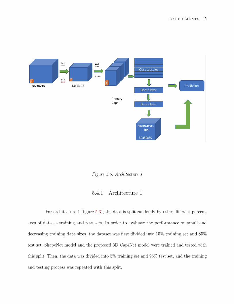
Figure 5.3: Architecture 1
5.4.1 Architecture 1
For architecture 1 (figure 5.3), the data is split randomly by using different percent-
ages of data as training and test sets. In order to evaluate the performance on small and
decreasing training data sizes, the dataset was first divided into 15% training set and 85%
test set. ShapeNet model and the proposed 3D CapsNet model were trained and tested with
this split. Then, the data was divided into 5% training set and 95% test set, and the training
and testing process was repeated with this split.

EXPERIMENTS 46
ShapeNet 3D CapsNetModelNet-10 84.37% 88.54%ModelNet-40 81.37% 82.61%
Table 5.3: ShapeNet versus 3D CapsNet using 15% of data for training.
ShapeNet 3D CapsNetModelNet-10 77.85% 83.21%ModelNet-40 73.47% 75.53%
Table 5.4: ShapeNet versus 3D CapsNet using 5% of data for training.
Table 5.3 shows the comparison of the results obtained from training the proposed
3D CapsNet and ShapeNet classifiers with 15% of the dataset for both ModelNet-10 and
ModelNet-40 datasets. Similarly, Table 5.4 shows the results obtained from training the
classifiers with 5% of the datasets. Our proposed 3D CapsNet performs better in all cases.
When Table 5.4 is compared with Table 5.3, it can be seen that the performance improvement
obtained with the 3DcapsNet is indeed more significant when training data size gets smaller.
For instance, with ModelNet-10 dataset, our proposed 3D CapsNet performs significantly
better than the ShapeNet after being trained on as little as 5% of the entire dataset. The
training data in this case contained as few as seven examples for a class. It should also be
noted that the default split provided on the ModelNet web page is 81.5% for training and
18.5% for testing for ModelNet-10 dataset, and 80% for training and 20% for testing for
ModelNet-40 dataset. This shows once more what a small percentage of data we used for
training in our experiments.
Finally table 5.5 shows the comparison of the results obtained from training the
proposed 3D CapsNet and ShapeNet classifiers with 40% of the dataset for both ModelNet-10

EXPERIMENTS 47
and ModelNet-40 datasets.
The results of all the 5 architectures have been summarized and compared in the
analysis subsection (Table 5.12).
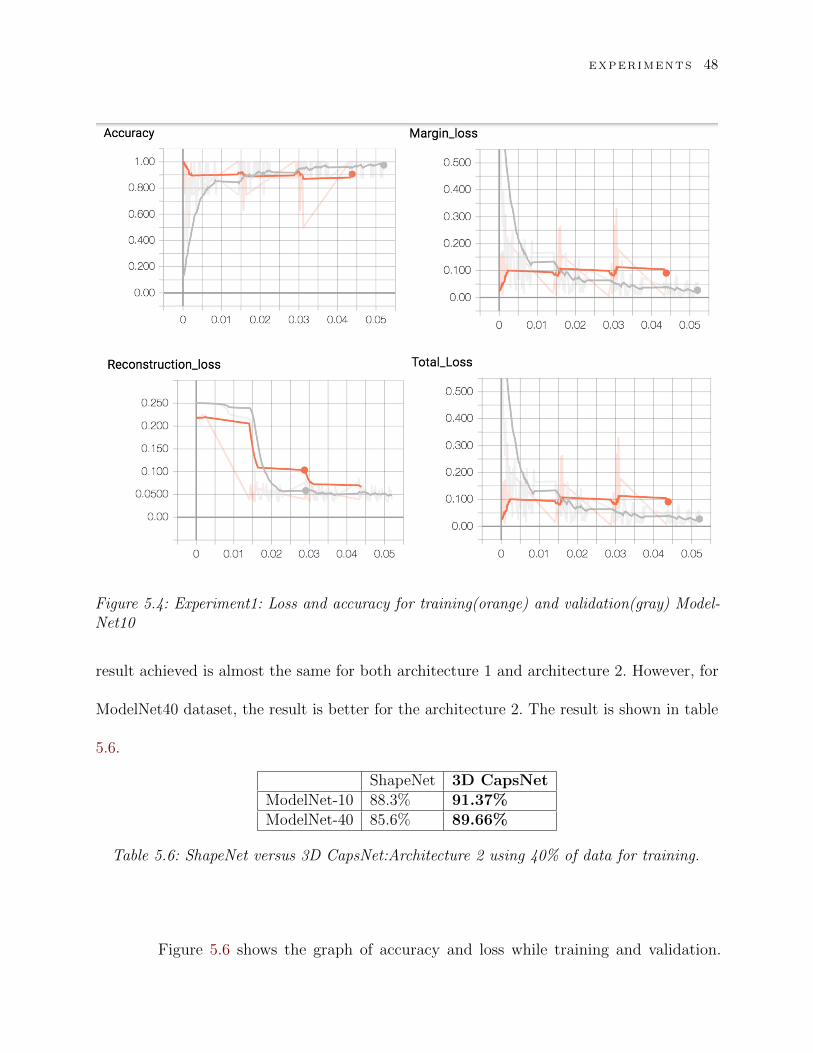
Figure 5.4 shows the graph of accuracy and loss while training and validation.
Training is shown by using orange and validation is shown with grey.
ShapeNet 3D CapsNetModelNet-10 88.3% 91.48%ModelNet-40 85.6% 88.67%
Table 5.5: ShapeNet versus 3D CapsNet: Architecture-1 using 40% of data for training.
5.4.2 Architecture 2
For this variation of CapsNet (figure 5.5), the data is divided into 40% for training
and the remaining data for test and validation. Just as architecture 2, the training data is
increased, yet kept lower than traditional model training to exhibit the property of CapsNet
being able to train using less data, since the default split provided on the ModelNet web page
is 81.5% for training and 18.5% for testing for ModelNet-10 dataset, and 80% for training
and 20% for testing for ModelNet-40 dataset. This shows once more what a small percentage
of data we used for training in our experiments. The results of all the 5 architectures have
been summarized and compared in the analysis subsection (Table 5.12).
Here instead of using pooling layer like the architecture 1, stride 2 has been used
to reduce the size of feature map to be input into primary capsule. For ModelNet10, the
EXPERIMENTS 48
Figure 5.4: Experiment1: Loss and accuracy for training(orange) and validation(gray) Model-Net10
result achieved is almost the same for both architecture 1 and architecture 2. However, for
ModelNet40 dataset, the result is better for the architecture 2. The result is shown in table
5.6.
ShapeNet 3D CapsNetModelNet-10 88.3% 91.37%ModelNet-40 85.6% 89.66%
Table 5.6: ShapeNet versus 3D CapsNet:Architecture 2 using 40% of data for training.
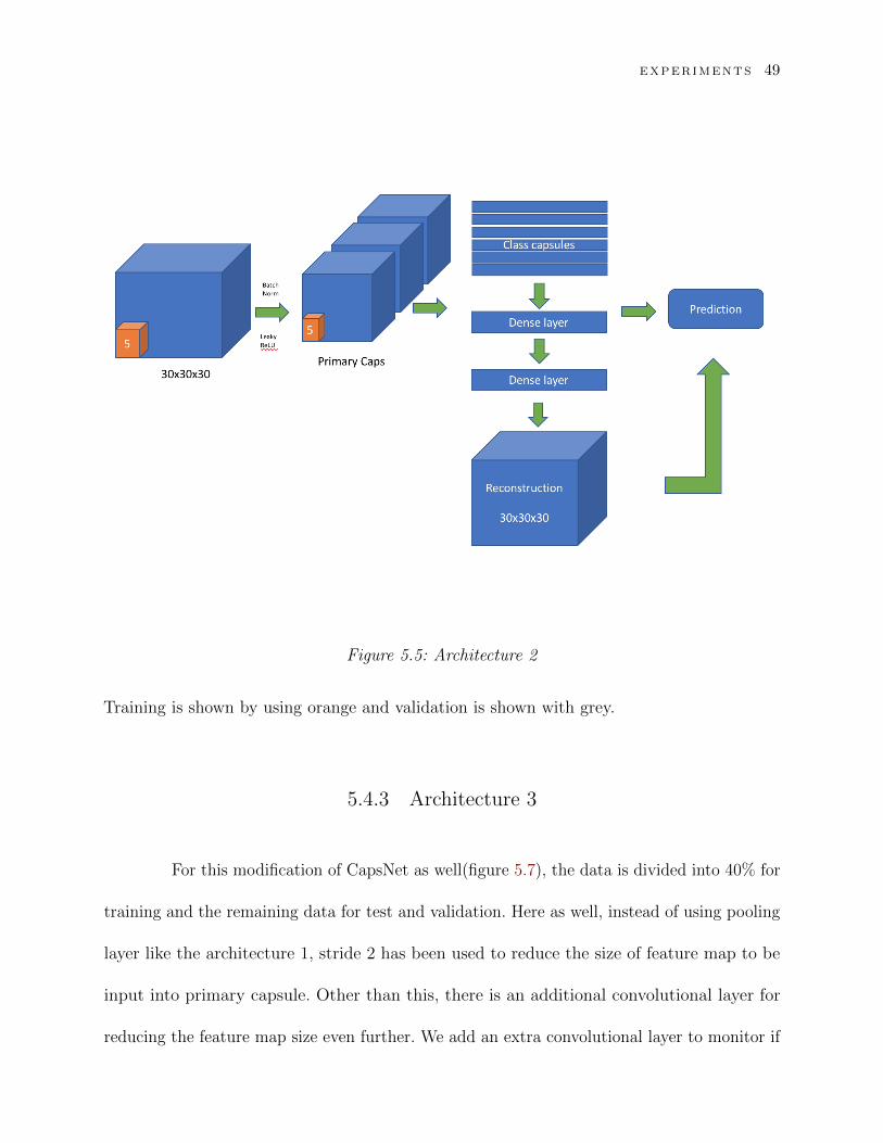
Figure 5.6 shows the graph of accuracy and loss while training and validation.
EXPERIMENTS 49
Figure 5.5: Architecture 2
Training is shown by using orange and validation is shown with grey.
5.4.3 Architecture 3
For this modification of CapsNet as well(figure 5.7), the data is divided into 40% for
training and the remaining data for test and validation. Here as well, instead of using pooling
layer like the architecture 1, stride 2 has been used to reduce the size of feature map to be
input into primary capsule. Other than this, there is an additional convolutional layer for
reducing the feature map size even further. We add an extra convolutional layer to monitor if

EXPERIMENTS 50
Figure 5.6: Experiment2: Loss and accuracy for training (orange) and validation (blue)ModelNet10
adding convolutional depth to the architecture adds value to the model’s performance. We
observe that, adding an additional layer does not truly add value to the model’s results. The
result is shown in table 5.7. The results of all the 5 architectures have been summarized and
compared in the analysis subsection (Table 5.12).
ShapeNet 3D CapsNetModelNet-10 88.3% 90.625%ModelNet-40 85.6% 87.28%
Table 5.7: ShapeNet versus 3D CapsNet:Architecture 3 using 40% of data for training.

EXPERIMENTS 51
Figure 5.7: Architecture 3
5.4.4 Architecture 4
The Architecture 4(Figure 5.9) has a similar architecture to Architecture 2. We
experiment with 64 filters in the convolution layer and removal of 1 dense layer in the decoder
section. Referring to table 5.8, we see that there is not a great difference between architecture
2 and architecture 4. In fact, lowering number of convolutional kernels and number of neurons
in the dense layer slightly reduces the test accuracy. Figure 5.10 shows the progress of learning
of this model.
EXPERIMENTS 52
Figure 5.8: Experiment3: Loss and accuracy for training(orange) and validation(blue) Model-Net10
5.4.5 Architecture 5
The Architecture 5 (Figure 5.11) is a variation with 2 primary capsules. We wish to
see if increasing the number of primary capsules affects learning of the model. Figure 5.12
shows the learning of this model. We see that the model learns in fewer epochs. The concern
with this model is that it take relatively more time to run. We get similar results as compared
to the other models.

EXPERIMENTS 53
Figure 5.9: Architecture 4
For this experiment, we first used 40% split to train the data. Since the model
performed well on 40% training data, we also used 5% split and 15% split to perform
experiments on the model. In table 5.9, we summarize the result of experiment on architecture
5 using 40% data. Next, in table 5.10, we summarize the result of experiment on architecture 5
using 15% data. Finally, in table 5.11, we summarize the result of experiment on architecture
5 using 5% data.
We summarize the results of all the architectures in the analysis section (Table 5.12).
We also compare the results of the experiment on architecture 1 and 5 with 5%, 15% and

EXPERIMENTS 54
ShapeNet Architecture 4 Architecture 2ModelNet-10 88.3% 90.75% 91.37ModelNet-40 85.6% 88.7% 89.66
Table 5.8: ShapeNet, 3D CapsNet:Architecture 4, 3D CapsNet:Architecture 2 using 40% ofdata for training.
Figure 5.10: Experiment4: Loss and accuracy for training (orange) and validation (blue)ModelNet10
40% data split in the analysis section (Table 5.13).

EXPERIMENTS 55
Figure 5.11: Architecture 5
5.5 Analysis
We observe from all the experiments that all these shallow models have similar
performances to each other. We have been able to achieve good results for shallow 3D CapsNet
architecture. The default split provided on the ModelNet web page is 81.5% for training
and 18.5% for testing for ModelNet-10 dataset, and 80% for training and 20% for testing for
ModelNet-40 dataset. However, we have randomly selected just 40% of the data and trained
our models on that.

EXPERIMENTS 56
ShapeNet 3D CapsNetModelNet-10 88.3% 91.31%ModelNet-40 85.6% 87.38%
Table 5.9: ShapeNet versus 3D CapsNet:Architecture-5 using 40% of data for training.
ShapeNet 3D CapsNetModelNet-10 84.37% 88.62%ModelNet-40 81.37% 82.7%
Table 5.10: ShapeNet versus 3D CapsNet:Architecture-5 using 15% of data for training.
Table 5.12 shows the comparison of results of all the different architectures. The
architecture 2 has overall highest accuracy(89.66% on test data) for ModelNet40. This shows
that a simple architecture with just 1 convolutional layer, 1 primary capsule layer, and 1
class layer, is also capable of learning and generalizing the 3D shapes admirably.
Table 5.13 shows result of test accuracies on ShapeNet, CapsNet architecture 1
and CapsNet architecture 5 models, trained with 5%, 15% and 40% training data. In all 3
ShapeNet 3D CapsNetModelNet-10 77.85% 83.79%ModelNet-40 73.47% 76.48%
Table 5.11: ShapeNet versus 3D CapsNet:Architecture-5 using 5% of data for training.
ModelNet10 ModelNet-40Architecture 1 91.48% 88.67%Architecture 2 91.37% 89.66%Architecture 3 90.625% 87.28%Architecture 4 90.75% 88.7%Architecture 5 91.30% 87.38%ShapeNet 88.3% 85.6%
Table 5.12: Summary: Comparison of proposed architectures and ShapeNet(40% training data)

EXPERIMENTS 57
Figure 5.12: Experiment5: Loss and accuracy for training(orange) and validation(blue) Mod-elNet10
scenarios, CapsNet performs better than ShapeNet. Between architecture 1 and architecture
5, we observe that for 5% and 15% training data, architecture 5 shows slightly better results.
This signifies that adding a primary capsule layer helps in reducing the amount of data
needed for training.
The accuracy for ModelNet-40 does not reach that of ModelNet10 due to that the
fact that some objects in 40 classes are just too challenging to be distinguished solely from
shapes. For example, “wardrobe” and “dresser”, “chair” and “bench”, “cone” and “tent”,
“plant” and “flower pot”, are all very similar in term of 3D shapes. It’s the appearance or

EXPERIMENTS 58
ModelNet-10 ModelNet-40
ShapeNetCapsNetArch 1
CapsNetArch 5
ShapeNetCapsNetArch 1
CapsNetArch 5
5% Training data 77.85% 83.21% 83.79% 73.47% 75.53% 76.48%15% Training data 84.37% 88.54% 88.62% 81.37% 82.61% 82.7%40% Training data 88.3% 91.48% 91.30% 85.6% 88.67% 87.38%
Table 5.13: Summary: Result of ShapeNet, Architecture 1 and Architecture 5 on different splitof dataset
the context that makes them different. The tasks using 40-categories are a lot harder not
only because of more categories, but also because the new classes are more challenging
to differentiate. This makes the performance upper limit much lower than the 10-category
experiments. Table 5.14 contains individual class accuracies of all the classes in ModelNet10.
Toilet, sofa, monitor, bed and chair have unique shapes. Thus, CapsNet realizes these shapes
better than the other shapes.

EXPERIMENTS 59
Arch1 Arch2 Arch3 Arch4 Arch5
Bathtub 72.72 79.8 78 78.87 75.43
Bed 93.89 94.17 94.21 92.17 93.19
Chair 99.59 98.5772 98.98 98.17 98.58
Desk 73.75 70.71 77.85 79.28 74.76
Dresser 75.83 81.75 87.84 80.4 78.5
Monitor 97.73 95.83 97.72 95.83 96.212
Night stand 76.81 71.81 72.46 84.05 86.96
Sofa 98.32 97.94 99.44 98.044 99.16
Table 85.08 78.07 75.43 92.017 75.43
Toilet 95.4 92.36 94.38 94.898 89.9
Table 5.14: Individual class accuracies (%) on ModelNet-10 with 40% training set.

CONCLUS ION AND FUTURE WORK 60
Chapter 6
Conclusion and Future Work
6.1 Conclusion
In this thesis, we have proposed 3D Capsule Network solutions to perform object
classification from 3D data which is present in the form of 3D binary occupancy grids. We have
proposed shallow architectures that can recognize shapes better than shallow architectures
based on pure convolutional networks. We have used 3D convolutional layers to extract the
features and proposed capsule architectures to identify the spatial relationships in the 3D
data better. We believe that this network provides a better representation to the human
vision system than pure convolutional neural network detectors.
It is claimed that Capsule Networks require less training data. We have been able
to prove this to be true for 3D data as well, in our experiments. We have compared our
approach with ShapeNet on the ModelNet dataset, and showed that our method provides
performance improvement especially when training data size gets smaller. With only 40%

CONCLUS ION AND FUTURE WORK 61
training data, we have been able to achieve close to 90% accuracy for ModelNet10 and close
to 88% for ModelNet40. We believe that our investigation steps a foot into the door to a new
area of research.
6.2 Limitations and future work
Though we have been able to provide a good architecture that works well with
volumetric data, there are few areas for improvements.
The current implementation of 3D capsule network is much slower than contemporary
deep learning model implementations in spite of having shallow architecture. This is due
large number of parameters that materialize due to the third dimension. And this causes
computational requirements to be very high. We made several optimizations to the original
capsule architecture to improve the speed of training. however, they were only able to do
so marginally. Thus, Performance optimization for capsules is an open-ended problem to be
solved.
Another limitation to current 3D capsule network, is its inability to be used in
production environments since it is still in the research phase. Though the concept of capsule
network for 3D data is intuitively appealing, the need for finding a robust implementation is
imperative. In our research, we have explored various solutions for solving the problem of
object recognition in 3D data using CapsNet. This is indeed, a solution worth enhancing.
Another future work recommendation is to improve regularization further for 3D

CONCLUS ION AND FUTURE WORK 62
data to avoid overfitting. This will enable the model to generalize better on smaller number
of 3D data.
With all these considerations, we can agree that there are myriads of opportunities
to develop capsule network to be able to utilize it to its full potential.

REFERENCES 63
References
[1] Geoffrey E Hinton, Alex Krizhevsky, and Sida D Wang. “Transforming auto-encoders”.
In: International Conference on Artificial Neural Networks. Springer. 2011, pp. 44–51
(cit. on pp. 3, 4, 18–21).
[2] Sara Sabour, Nicholas Frosst, and Geoffrey E Hinton. “Dynamic routing between
capsules”. In: Advances in Neural Information Processing Systems. 2017, pp. 3859–3869
(cit. on pp. 3, 4, 19, 24, 28, 30).
[3] Yann LeCun. “The MNIST database of handwritten digits”. In: http://yann. lecun.
com/exdb/mnist/ (1998) (cit. on p. 4).
[4] Alex Krizhevsky, Vinod Nair, and Geoffrey Hinton. “The CIFAR-10 dataset”. In: online:
http://www. cs. toronto. edu/kriz/cifar. html (2014) (cit. on p. 4).
[5] Yann LeCun, Fu Jie Huang, and Leon Bottou. “Learning methods for generic object
recognition with invariance to pose and lighting”. In: Computer Vision and Pattern
Recognition, 2004. CVPR 2004. Proceedings of the 2004 IEEE Computer Society
Conference on. Vol. 2. IEEE. 2004, pp. II–104 (cit. on p. 4).
[6] Alexander Andreopoulos and John K Tsotsos. “50 years of object recognition: Directions
forward”. In: Computer Vision and Image Understanding 117.8 (2013), pp. 827–891

REFERENCES 64
(cit. on p. 5).
[7] Stuart C Shapiro. Encyclopedia of artificial intelligence second edition. John, 1992
(cit. on p. 5).
[8] HG Barrow, JM Tenenbaum, AR Hanson, and EM Riseman. Computer vision systems.
1978 (cit. on p. 5).
[9] Isidore Rigoutsos and Robert Hummel. “A Bayesian approach to model matching
with geometric hashing”. In: Computer vision and image understanding 62.1 (1995),
pp. 11–26 (cit. on p. 5).
[10] Haim J Wolfson and Isidore Rigoutsos. “Geometric hashing: An overview”. In: IEEE
computational science and engineering 4.4 (1997), pp. 10–21 (cit. on p. 5).
[11] Svetlana Lazebnik, Cordelia Schmid, and Jean Ponce. “Semi-local affine parts for object
recognition”. In: British Machine Vision Conference (BMVC’04). The British Machine
Vision Association (BMVA). 2004, pp. 779–788 (cit. on p. 5).
[12] Hiroshi Murase and Shree K Nayar. “Visual learning and recognition of 3-D objects
from appearance”. In: International journal of computer vision 14.1 (1995), pp. 5–24
(cit. on p. 5).
[13] Chien-Yuan Huang, Octavia I Camps, and Tapas Kanungo. “Object recognition using
appearance-based parts and relations”. In: Computer Vision and Pattern Recognition,
1997. Proceedings., 1997 IEEE Computer Society Conference on. IEEE. 1997, pp. 877–
883 (cit. on p. 5).
[14] King-Sun Fu. “A step towards unification of syntactic and statistical pattern recogni-
tion”. In: IEEE transactions on pattern analysis and machine intelligence 3 (1986),
pp. 398–404 (cit. on p. 5).
REFERENCES 65
[15] Michael Leyton. “A process-grammar for shape”. In: Artificial Intelligence 34.2 (1988),
pp. 213–247 (cit. on p. 5).
[16] Tony Lindeberg. “Scale invariant feature transform”. In: Scholarpedia 7.5 (2012),
p. 10491 (cit. on pp. 5, 19).
[17] David G Lowe. “Object recognition from local scale-invariant features”. In: Computer
vision, 1999. The proceedings of the seventh IEEE international conference on. Vol. 2.
Ieee. 1999, pp. 1150–1157 (cit. on p. 5).
[18] Herbert Bay, Tinne Tuytelaars, and Luc Van Gool. “Surf: Speeded up robust features”.
In: European conference on computer vision. Springer. 2006, pp. 404–417 (cit. on p. 5).
[19] Daniel D Lee and H Sebastian Seung. “Learning the parts of objects by non-negative
matrix factorization”. In: Nature 401.6755 (1999), p. 788 (cit. on p. 5).
[20] Svante Wold, Kim Esbensen, and Paul Geladi. “Principal component analysis”. In:
Chemometrics and intelligent laboratory systems 2.1-3 (1987), pp. 37–52 (cit. on p. 5).
[21] Fernando De la Torre and Michael J Black. “Robust principal component analysis for
computer vision”. In: Computer Vision, 2001. ICCV 2001. Proceedings. Eighth IEEE
International Conference on. Vol. 1. IEEE. 2001, pp. 362–369 (cit. on p. 5).
[22] Sergey Ioffe. “Probabilistic linear discriminant analysis”. In: European Conference on
Computer Vision. Springer. 2006, pp. 531–542 (cit. on p. 5).
[23] Zhouyu Fu and Antonio Robles-Kelly. “Learning object material categories via pairwise
discriminant analysis”. In: Computer Vision and Pattern Recognition, 2007. CVPR’07.
IEEE Conference on. IEEE. 2007, pp. 1–7 (cit. on p. 5).
[24] Daniel L Swets and Juyang Weng. “Discriminant analysis and eigenspace partition
tree for face and object recognition from views”. In: Automatic Face and Gesture

REFERENCES 66
Recognition, 1996., Proceedings of the Second International Conference on. IEEE. 1996,
pp. 192–197 (cit. on p. 5).
[25] Alex Krizhevsky, Ilya Sutskever, and Geoffrey E Hinton. “Imagenet classification with
deep convolutional neural networks”. In: Advances in neural information processing
systems. 2012, pp. 1097–1105 (cit. on p. 5).
[26] Jonathan Masci, Davide Boscaini, Michael Bronstein, and Pierre Vandergheynst.
Shapenet: Convolutional neural networks on non-euclidean manifolds. Tech. rep. 2015
(cit. on pp. 5, 14, 44).
[27] Daniel Maturana and Sebastian Scherer. “Voxnet: A 3d convolutional neural network
for real-time object recognition”. In: Intelligent Robots and Systems (IROS), 2015
IEEE/RSJ International Conference on. IEEE. 2015, pp. 922–928 (cit. on pp. 5, 14).
[28] Wanli Ouyang, Xingyu Zeng, Xiaogang Wang, Shi Qiu, Ping Luo, Yonglong Tian,
Hongsheng Li, Shuo Yang, Zhe Wang, Hongyang Li, et al. “DeepID-Net: Object
Detection with Deformable Part Based Convolutional Neural Networks”. In: IEEE
Transactions on Pattern Analysis and Machine Intelligence 39.7 (2017), pp. 1320–1334
(cit. on p. 8).
[29] Matthew D Zeiler and Rob Fergus. “Stochastic pooling for regularization of deep
convolutional neural networks”. In: arXiv preprint arXiv:1301.3557 (2013) (cit. on
pp. 9, 10).
[30] Kaiming He, Xiangyu Zhang, Shaoqing Ren, and Jian Sun. “Spatial pyramid pooling
in deep convolutional networks for visual recognition”. In: european conference on
computer vision. Springer. 2014, pp. 346–361 (cit. on p. 9).
[31] Christian Szegedy, Wei Liu, Yangqing Jia, Pierre Sermanet, Scott Reed, Dragomir

REFERENCES 67
Anguelov, Dumitru Erhan, Vincent Vanhoucke, and Andrew Rabinovich. “Going Deeper
with Convolutions”. In: Computer Vision and Pattern Recognition (CVPR). 2015. ur l :
http://arxiv.org/abs/1409.4842 (cit. on p. 9).
[32] Geoffrey E Hinton and Ruslan R Salakhutdinov. “Reducing the dimensionality of data
with neural networks”. In: science 313.5786 (2006), pp. 504–507 (cit. on p. 10).
[33] Mostafa Abdel. “3D LASER SCANNERS: HISTORY, APPLICATIONS, AND FU-
TURE”. In: (2011) (cit. on p. 11).
[34] Benjamin Adams and Krzysztof Janowicz. “On the Geo-Indicativeness of Non-Georeferenced
Text.” In: ICWSM. 2012, pp. 375–378 (cit. on p. 11).
[35] O Fernandez. “Obtaining a best fitting plane through 3D georeferenced data”. In:
Journal of Structural Geology 27.5 (2005), pp. 855–858 (cit. on p. 11).
[36] Kresimir Kusevic, Paul Mrstik, and Craig Len Glennie. Method and system for aligning
a line scan camera with a lidar scanner for real time data fusion in three dimensions.
US Patent App. 12/642,144. June 2010 (cit. on p. 12).
[37] Chris McGlone, Edward Mikhail, and Jim Bethel. “Manual of photogrammetry”. In:
(1980) (cit. on p. 12).
[38] Fred W DePiero and Mohan M Trivedi. “3-D computer vision using structured light:
Design, calibration, and implementation issues”. In: Advances in computers. Vol. 43.
Elsevier, 1996, pp. 243–278 (cit. on p. 12).
[39] Zhengyou Zhang. “Microsoft kinect sensor and its effect”. In: IEEE multimedia 19.2
(2012), pp. 4–10 (cit. on p. 12).
[40] Steven G Schock, Arnaud Tellier, Jim Wulf, Jason Sara, and Mark Ericksen. “Buried
object scanning sonar”. In: IEEE journal of oceanic engineering 26.4 (2001), pp. 677–
REFERENCES 68
689 (cit. on p. 12).
[41] Michael Stark, Michael Goesele, and Bernt Schiele. “Back to the Future: Learning
Shape Models from 3D CAD Data.” In: Bmvc. Vol. 2. 4. Citeseer. 2010, p. 5 (cit. on
p. 12).
[42] Du Tran, Lubomir Bourdev, Rob Fergus, Lorenzo Torresani, and Manohar Paluri.
“Learning spatiotemporal features with 3d convolutional networks”. In: Computer Vision
(ICCV), 2015 IEEE International Conference on. IEEE. 2015, pp. 4489–4497 (cit. on
p. 14).
[43] Charles R Qi, Hao Su, Matthias Nießner, Angela Dai, Mengyuan Yan, and Leonidas J
Guibas. “Volumetric and multi-view cnns for object classification on 3d data”. In:
Proceedings of the IEEE conference on computer vision and pattern recognition. 2016,
pp. 5648–5656 (cit. on p. 16).
[44] Varun Arvind, Anthony Costa, Marcus Badgeley, Samuel Cho, and Eric Oermann.
“Wide and deep volumetric residual networks for volumetric image classification”. In:
arXiv preprint arXiv:1710.01217 (2017) (cit. on p. 16).
[45] Geoffrey Hinton, Nicholas Frosst, and Sara Sabour. “Matrix capsules with EM routing”.
In: (2018) (cit. on pp. 19, 22, 23).
[46] Carl Edward Rasmussen. “The infinite Gaussian mixture model”. In: Advances in
neural information processing systems. 2000, pp. 554–560 (cit. on p. 22).
[47] Angel X Chang, Thomas Funkhouser, Leonidas Guibas, Pat Hanrahan, Qixing Huang,
Zimo Li, Silvio Savarese, Manolis Savva, Shuran Song, Hao Su, et al. “Shapenet: An
information-rich 3d model repository”. In: arXiv preprint arXiv:1512.03012 (2015)
(cit. on p. 41).

Ayesha AhmadCurriculum Vitae
PERSONAL DETAILS
Birth April 19, 1992
Address 416 Columbus Ave, Syracuse
Phone (315) 949-8687
Mail [email protected]
EDUCATION
MSc. Computer Science 2016-2018Syracuse University
GPA- 3.68
Relevant Coursework- Machine Intelligence and Deep Learning, Artificial Intelligence, Object
Oriented Design, Design and Analysis of Algorithms, Natural Language Processing
B. Engg Information Science and Engineering 2010-2014Visvesvaraya Technological University
MASTER THESIS
Object Recognition in 3D data using Capsules 2018Supervisor- Dr. Senem Velipasalar
Proposed techniques to recognize objects in 3D volumetric data
WORK EXPERIENCE
Machine Learning and Computer Vision Engineer Intern 2018- present
Quantifly LLC, Part-time
• Planning and preparing a road map for research and development with Quantifly engineeringteam
• Building a research and development schedule for Quantifly engineering team
Software Developer Intern 2017Capella Education Company, Full-time
• Developed an in-house tool called browser check using Adobe Experience Manager andJavaScript
• Interacted with business stakeholders to gather requirements such as screen resolution,platform info, browser plugin info, etc.
• Worked on Change request user stories during the website’s Visitor Center update byrewriting backend AEM logic using JAVA.
Software Developer 2014-2016Sapient Nitro, Full-time
• Worked as a developer specializing in E-commerce software development for several multi-million-dollars clients.
• Worked with Hybris Platform for E-commerce backend development using Advanced JAVAand Spring framework.
• Worked in a cross functional team by interacting with business analysts, front end developersand QA team ensuring robust development.
Software Intern 2014Aricent Technology, Full-time
• Worked on a product called Aricloud, a management and monitoring tool for heterogeneouscloud environments such as AWS, Azure, etc
• Worked with Hybris Platform for E-commerce backend development using Advanced JAVAand Spring framework.
• Developed and tested several key modules and integrated them with Cloud services RESTAPIs.
PROJECTS
Natural language processing and Sentiment analysis 2017
• Implemented a sentiment classifier to categorize processed tweets into ”positive”,”negative” and ”neutral” using NLTK and Sci-kit learn.
Object recognition in images for CIPHAR-10 dataset 2017
• Implemented 2-layer Neural Network, SVM and Softmax classifiers in Python withNumpy package.
• Implemented 5-layer convolutional neural network using Tensorflow.
• Implemented Capsule network using Tensorflow.
Comparison of the maturity of bloggers of different age groups using theirblog posts 2017
• Compared the maturity levels of teenagers and adults in their 40s by analyzing theirvocabulary and topics that they choose for writing.
• Used Python and NLTK to perform this analysis after extracting blogs from theBlogger corpus.
Survival prediction on the Titanic using Kaggle dataset 2017
• Performed feature engineering to clean the data and predicted whether an individualwould survive or not with accuracy of 77.5 %.
• Implemented random forest algorithm using R programming.
SKILLS
ProgrammingLanguages
Python, JAVA, J2EE, C, C++, R programming, MATLAB
Web pro-gramming
HTML5, CSS3, JavaScript, JQuery, Ajax
OperatingSystems
Linux, Ubuntu, Windows, iOS, Unix
Databases MySQL
Other UML, Data Structures, Tensor Flow, Scikit-learn, NLTK, Git
Frameworks Spring, Hybris