Objective Functions

Guiding

Adaptive Neurodynamics

Claudius GrosRodrigo Echeveste, Mathias Linkerhand,Hendrik Wernecke, Valentin Walther

Institute for Theoretical PhysicsGoethe University Frankfurt, Germany

1

concepts

generating functionals

Kullback-Leibler divergenceFisher information

intrinsic adaptionsynaptic plasticity

attractor metadynamicsself-organized fading memory

2

the control problem

model building for complex systems

∗ potentially large numbers of control parameters

∗ high dimensional phase space

physical / biologicalinsights

higher-level principlegenerating functional

︸ ︷︷ ︸

equations of motion = . . .

3

time allocation of neural activity

firing-rate distribution

p(y) =1

T

∫ T

0

δ(y− y(t − τ))dτ

time

firi

ng

rat

e y

(t)

information-theoretical objectives

maximal information stationarity with respect

transmisssion to synaptic weights

Kullback-Leibler divergence Fisher information

4

rate encoding neuron

y =1

1+ exp((b− ))

: ginb : bis

�����

������

������� �������� ��������

intrinsic plasticity

maximal information transmission

⇓

adapt gain and bias b

5

maximal information distribution

Shannon entropy H[p] = −⟨ logp ⟩

no constraints → p(y) ∼ const.

given mean μ → pμ(y) ∼ exp(−y/μ), μ =∫

yp(y)dy

• target firing-rate distribution pμ(y) (polyhomeostasis)

Kullback-Leibler divergence

D(p, pμ) =

∫

p(y) log

�p(y)

pμ(y)

�

dy ≥ 0

• asymmetric measure for the distanceof two probability distribution functions

6

stochastic adaption rules

functional dependence on input statistics

• distributions of input / output p() / p(y)

D =

∫

p(y) log

�p(y)

pμ(y)

�

dy ≡

∫

p()d()d

with

p(y)dy = p()d, d() ≡ log(p)− log(∂y/∂)− log(pμ)

adaption rules: ∀ input statistics

[ δD = 0, ∀p() ] =⇒ δd = 0

7

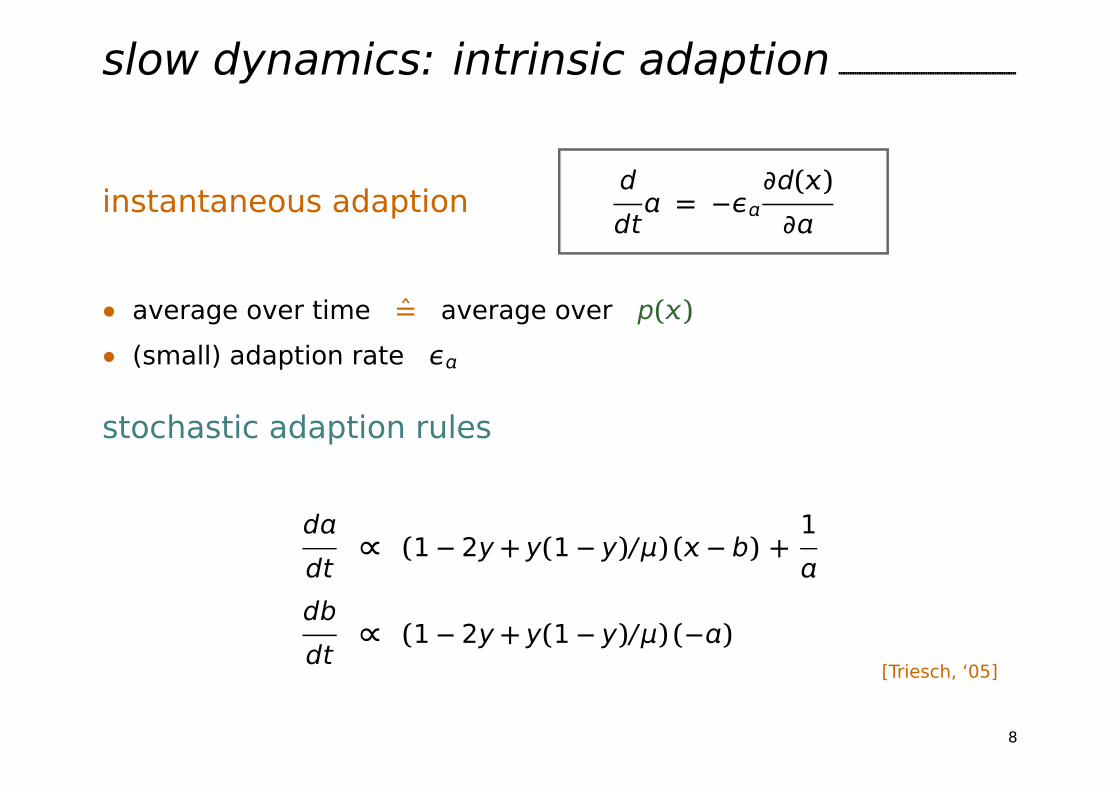
slow dynamics: intrinsic adaption

instantaneous adaptiond

dt = −ε

∂d()

∂

• average over time = average over p()

• (small) adaption rate ε

stochastic adaption rules

d

dt∝ (1− 2y+ y(1− y)/μ) (− b) +

1

db

dt∝ (1− 2y+ y(1− y)/μ) (−)

[Triesch, ‘05]

8

autapse: self-coupled neuron

[Markovic & Gros, PRL ‘10]

1000 2000 3000

time

0

1

2

3

par

amet

ers,

o

utp

ut a(t)-4

b(t)y(t) y

x

a, b

polyhomeostatic optimization inducescontinuous, self-contained neural activity

attractor network  limit cycle

9

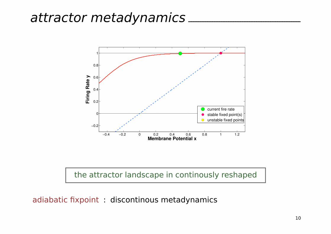
attractor metadynamics

the attractor landscape in continously reshaped

adiabatic fixpoint : discontinous metadynamics

10

−0.4 −0.2 0 0.2 0.4 0.6 0.8 1 1.2

−0.2

0

0.2

0.4

0.6

0.8

1

Membrane Potential x

Fir

ing

Rate

y

current fire rate

stable fixed point(s)

unstable fixed points

attractor competition

three-site network

−→ : exitatory, j = +1−→ : inhibitory, j = −1

two possible attractors(1,1,0) (0,1,1)

attractor network ⇔ slow polyhomeostatic adaption

11

activity of neuron one/three

adiabatic fixpoint : limit cycle

neural dynamics : slowing down at attractor relicts 12

0 0.2 0.4 0.6 0.8 10

0.2

0.4

0.6

0.8

1

Firing Rate y1

Fir

ing

Rate

y3

current state

(stable) fixed point(s)

attractor relict networks

!!!!!!!!!!!!!!!!!!!!!!!!!!!!!!!!!!!!!!!!!!!!!!!!!!!!!!!!!!!!!!!!!!!!!!!!!!!!!!!!!!!!!!!!!!!!!!!!!!!!!!!!!!!!!!!!!!!!!!!!!!!!!!!!!!!!!!!!!!!!!!!!!!!!!!!!!!!!!!!!!!!!!!!!!!!!!!!!!!!!!!!!!!!!!!!!!!!!!!!!!!!!!!!!!!!!!!!!!!!!!!!!!!!!!!!!!!!!!!!!!!!!!!!!!!!!!!!!!!!!!!!!!!!!!!!!!!!!!!!!!!!!!!!!!!!!!!!!!!!!!!!!!!!!!!!!!!!!!!!!!!!!!!!!!!!!!!!!!!!!!!!!!!!!!!!!!!!!!!!!!!!!!!!!!!!!!!!!!!!!!!!!!!!!!!!!!!!!!!!!!!!!!!!!!!!!!!!!!!!!!!!!!!!!!!!!!!!!!!!!!!!!!!!!!!!!!!!!!!!!!!!!!!!!!!!!!!!!!!!!!!!!!!!!!!!!!!!!!!!!!!!!!!!!!!!!!!!!!!!!!!!!!!!!!!!!!!!!!!!!!!!!!!!!!!!!!!!!!!!!!!!!!!!!!!!!!!!!!!!!!!!!!!!!!!!!!!!!!!!!!!!!!!!!!!!!!!!!!!!!!!!!!!!!!!!!!!!!!!!!!!!!!!!!!!!!!!!!!!!!!!!!!!!!!!!!!!!!!!!!!!!!!!!!!!!!!!!!!!!!!!!!!!!!!!!!!!!!!!!!!!!!!!!!!!!!!!!!!!!!!!!!!!!!!!

θ jj{x (t), (t)}

θ = 0jj

{x (t), }

adaption processes destroy stable fixpoints

transient synaptic plasticity, intrinsic plasticity, ..

– reservoir dynamics –︸ ︷︷ ︸

attractors turn into attractor relicts

13

transient state dynamics

j =1

Np

∑

α

ξ(α)

ξ(α)

j

for convenienceHopfield patterns: ξ

(α)

overlap firing y – ξ(α)

patterns[Linkerhand & Gros, MMCS ‘13]

14

competing objective functions

bursting transient state dynamics

target activtiy μ = 0.15

⟨ξ(α)

⟩ = 0.3 mean activity of attractors

⇒ guiding self-organization[Prokopenko ‘09]

15

stationarity of firing-rate distribution

pn = p(y1, y2, . . .)p

out= p(y)

w1

w2 pot = p(y)

lerning completed

dtn = 0

⇐⇒pot sttionry

∂

∂npot = 0

=⇒ Hebbian learning rules

16

Fisher information

Fθ =

∫

dypθ(y)

�∂

∂θlogpθ(y)

�2

measures the sensibility of aprobability distribution pθ(y)

with respect to a parameter θ

Cramer-Rao bound

D�

θ− θ�2E

≥1

Fθ

for the estimate θof an external parameter θ

» not used here «

17

minimization of Fisher information

leads to equations of motions / adaption rules[Reginatto, PRA ‘88]

minimizing the Fisher information of p() = |ψ(, t)|2

plus the continuity equationyields the Schrödinger equation

stationarity of firing-rate distribution

minimizing the Fisher information of the neuraloutput activity with respect to synaptic weights

leads to Hebbian learning rules

18

synaptic flux operator

∂

∂θ=∑

j

j

∂

∂j

= w · ∇

afferent synaptic weight j

rotationally invariantdimensionless

Fθ =∫

dyp(y)�

∂

∂θlogp(y)�2

F =∫

dyp(y)�∑

jj∂

∂jlogp(y)�2

F : sensitivity of firing rate with respectto changes of the j

19

self-limiting Hebbian

j = εG()H()(yj − yj)G() = 2+ (1− 2y)H() = (2y− 1) + 2(1− y)y

weak/strong postsynaptic activity

j ∝

�(2+ ) (−1) (yj − yj) (y→ 0)(2− ) (+1) (yj − yj) (y→ 1)

.

|| < 2 Hebbian

|| > 2 anti-Hebbian

=∑

j

j (yj − yj)

21

emergent fading memory

synaptic fluxoptimization

(c) noprincipal component

Oja’s rule

(a) along y1

(b) along y2

(d) along y3

���

�

��

�

��

��

��

��

��

�

�

��

��

���

�

� � � � �

� ����

��

�

�

�

��������� ����������

� �

23

outlook

decision making in the brain

(A) (B)

??

x(t)

??

x(t)

(A) (B)

competing generating functionals

• distinct objective functions cannot be merged

complex system ≡ competing objectives?

24

conclusions

generating functionals

• controlling dynamical states

 chaos / intermittent bursting / synchronization

attractor metadynamics

• induced by slow apdation processes

 adiabatic attractor landscape

synaptic plasticity

• beyond principal component analysis

 self-organized fading memory / binary classification

25

graduate level textbook

[Springer 2008,

third edition 2013]

Complex and AdaptiveDynamical Systems, a Primer

• The small world phenomenon insocial and scale-free networks

• Phase transitions andself-organized criticality

• Life at the edge of chaos andcoevolutionary avalanches

• Living dynamical systemsand emotional diffusive controlwithin cognitive system theory

26