objective identification and multi-scale controlling

atmosphere

Article

Objective Identification and Multi-Scale ControllingFactors of Extreme Heat-Wave Events inSouthern China

Wenjiang Chen 1,2,3, Joshua-Xiouhua Fu 1,3,* and Guoping Li 2

1 Department of Atmospheric & Oceanic Sciences and Institute of Atmospheric Sciences, Fudan University,Shanghai 200438, China; [email protected]

2 School of Atmospheric Sciences, Chengdu University of Information Technology, Chengdu 610225, China;[email protected]

3 Innovation Center of Ocean and Atmosphere System, Zhuhai Fudan Innovation Research Institute,Zhuhai 518057, China

* Correspondence: [email protected]

Received: 1 May 2020; Accepted: 19 June 2020; Published: 23 June 2020��

Abstract: Southern China (SC) is often subjected to the impacts of extreme heat-wave (EHW) eventswith hot days covering large areas and lasting extended periods in the boreal summer. The presentstudy explores new objective identification methods of the EHW events and reveals the controllingfactors of different spatial-temporal variations in shaping the EHW events over SC from 2000 to2017 with in-situ observations and latest reanalysis. A compound index of the EHW (with impactarea, duration, and magnitude) was defined to quantify the overall intensity of the EHW events inSC. It was found that synoptic variability and 10–30-day intra-seasonal variability (ISV) induce theonsets of the EHW events, while 30–90-day ISV shapes the durations. An innovative daily compoundindex was introduced to track the outbreak of the EHW events. The occurrences of the EHW in SCare coincident with the arrivals of intra-seasonal signals (e.g., the anomalies of outgoing long-waveradiation (OLR) and 500 hPa geopotential height) propagating from the east and south. About 12 daysbefore the onset of the EHW in SC, the 10–30-day positive anomalies of 500 hPa geopotential heightand OLR appear near the equatorial western Pacific, which then propagate northwestward to initiatethe EHW in SC. At the same time, the 30–90-day suppressed phase propagates northeastward fromthe Indian Ocean to the SC to sustain the EHW events. On the interannual time scale, it was foundthat the EHW events in SC occurred in those years with robust warming of the western North Pacificin early summer (May and June) and warming of the equatorial eastern Pacific in the precedingwinter (December, January, and February). An interannual sea surface temperature anomalous (SSTA)index, which adds together the SSTA over the above two regions, serves as a very useful seasonalpredictor for the EHW occurrences in SC at least one-month ahead.

Keywords: extreme heat-wave (EHW) events; objective identification; multi-scale controlling factors;Southern China (SC)

1. Introduction

A recent World Meteorological Organization report [1] has clearly shown that, in associationwith global warming, the occurrences of extreme meteorological events have increased steadily inpast decades. These extreme events have caused tremendous economic and societal losses around theworld and are threatening the sustainable development of global society. To better understand theprocesses controlling these extreme events and to develop advanced prediction capability for theseextremes are forefront grand challenges faced by the global meteorological community.

Atmosphere 2020, 11, 668; doi:10.3390/atmos11060668 www.mdpi.com/journal/atmosphere

http://www.mdpi.com/journal/atmosphere

http://www.mdpi.com

https://orcid.org/0000-0001-5025-0081

http://www.mdpi.com/2073-4433/11/6/668?type=check_update&version=1

http://dx.doi.org/10.3390/atmos11060668

http://www.mdpi.com/journal/atmosphere

Atmosphere 2020, 11, 668 2 of 19

In China, the frequent occurrences of large-scale events with air temperature exceeding 35 ◦Cand the resulting disasters have drawn great attention of governments and the meteorologicalcommunity [2,3]. Heat-waves, which have occurred in many places of China, with such high airtemperature, widespread extent, and prolonged duration are extremely harmful,. For example, in the2003 summer, a severe heat-wave occurred over a large area from the south of the Yangtze River to themiddle of Southern China (SC), which caused tremendous stresses on the local transportation, water,electricity and other urban operational lifelines as well as societal and economic activities [2]. For sucha heat-wave event, the days with maximum air temperature exceeding 38 ◦C are 5–20-days more thanthe climatology. In the 2013 summer, another severe heat-wave hit the Yangtze River Basin of China,resulting in direct economic loss amounting to 59 billion Chinese Yuan [3].

Unlike visible, destructive and violent extreme meteorological events (e.g., floods, tropical cyclonesand tornadoes etc.), the Extreme-Heat-Wave (EHW) events exert great threats to society and humanhealth in an unconscious way, thus gaining the nickname of “silent killer”. Due to the complexmulti-scale processes involved in the making of extreme meteorological events [2,4–7] and the chaoticnature of the atmosphere, it is very difficult to predict the extreme events accurately with sufficient leadtimes, which brings many restrictions to effective disaster prevention and reduction [1]. Therefore, it isof great scientific and societal implication to better understand the controlling factors and predictabilityof the EHW. Many previous studies have investigated the respective impacts of synoptic weathersystems, subseasonal-to-seasonal, and interannual-to-decadal variations on the heat-wave.

On the synoptic time scale, Ding and Qian [2] pointed out that the synoptic precursors of theheat-wave in China can be found from the 250 hPa continent-scale geopotential height anomalies, whichmove westward in low latitudes and east-southeastward in middle latitudes; for SC, the precursorsfrom the northwest Pacific have an averaged lead time of 4.6 days, the precursors initiated over Europeand northwest China have lead times ranging from 2 to 15 days. Wang et al. [4] found that East-AsianEHW events are strongly associated with the “exit” and the “tail” regions of the East-Asian jet stream.Poleward displacement of the jet-exit region is associated with warming tropospheric air temperaturesover East Asia and tends to be linked with high EHW frequency, while enhancement of the tail isassociated with cooling tropospheric air temperatures in the northern Pacific and tends to be linkedwith low EHW frequency. Li et al. [8] attributed the 2013 summer heat-wave to a result of the westwardextensions of the stable and strong western Pacific subtropical high. In this summer, there were fourwestward pulses of western Pacific subtropical high, which directly led to four heat-wave periods overthe SC. Wang et al. [9] pointed out that the coupling between the westward-enhanced western Pacificsubtropical high and the poleward-displaced East-Asian jet stream blocked the moisture supply fromthe southwest monsoon, resulting in the eastern China heat-wave in 2013. Chen et al. [10] found thatwhen the atmosphere is in a quasi-barotropic state, it is easier to form widespread persistent high airtemperature weather systems. Loikith and Broccoli [11] showed that warm extremes at most locationsin North America are associated with wavy patterns: Positive 500 hPa geopotential height and sealevel pressure anomalies in the downstream along with negative anomalies farther upstream.

On subseasonal-to-seasonal time scales, Chen et al. [5] pointed out that the daily air temperatureand circulation anomalies over the SC exhibit fluctuations with a period of about 10 days, largelyresulting from the influence of quasi-biweekly oscillation, which originates from the tropical westernPacific and propagates northwestward. The biweekly oscillation explains more than 50% of the5–25-day variance of daily maximum air temperature and vorticity over SC and 80% of heat-wave onsettiming. Gao et al. [12] found that when a significantly low-level anticyclonic anomaly associated withbiweekly oscillation appears over the Yangtze River valley, air temperature rises sharply due to theadiabatic heating associated with subsidence and the enhanced downward solar radiation associatedwith reduced clouds. Diao et al. [13] pointed out that when the positive rainfall anomaly of theboreal-summer intraseasonal oscillation is primarily located over a northwest–southeast-oriented beltextending from India to Maritime Continent and a negative rainfall anomalous belt exists in southeastAsia and western North Pacific, the occurrence probability of EHW events in the Asian-Pacific sector

Atmosphere 2020, 11, 668 3 of 19

is significantly elevated. Chen et al. [6] found that the fluctuating anomalies of daily maximumair temperature over SC and the western Pacific are intimately related to two intraseasonal modes,namely, the 5–25-day and 30–90-day oscillations, which originate from the tropical western Pacific andpropagate northwestward. The 5–25-day oscillation is vital in triggering and terminating the heat-wave,accounting for approximately 50% transitions of the daily air temperature and circulation anomaliesin the raw time series. The 30–90-day oscillation favors the persistent warming during heat-waveevents, accounting for approximately one-third of the prolonged warming and anticyclonic anomalies.Chen and Zhai [14] indicated that the boreal-summer intraseasonal oscillation can simultaneouslyfacilitate precipitation extremes in central-eastern China and EHW events in southern and southeastChina. It is the overturning circulation of the boreal-summer intraseasonal oscillation, with ascendingmotion in the Yangtze-Huai River Basin and descending motion in the south, that results in thesimultaneous, but opposite extremes.

On interannual-to-decadal time scales, Ding et al. [15] indicated that, over most of China exceptnorthwestern China, the frequency of the heat-wave exhibits a high-low-high fluctuating pattern,respectively, for the 1960s–1970s, 1980s, and afterwards. A remarkable upward trend of the heat-waveexists after the 1990s over entire China. It is also found that the interannual-to-interdecadal variationsof the heat-wave are closely related to the variations of rainy days and atmospheric circulation patterns.On the decadal time scale, Chen et al. [16] found that the relationships among the SC air temperature,large-scale atmospheric circulation pattern over the Eurasia and the tropical sea surface temperatureanomaly (SSTA) experienced a decadal shift around the early 1990s. Before the early 1990s, the warmersummer in SC largely originated from teleconnection from high latitude, which is featured by higherpressure over the Ural Mountains and the Korean Peninsula and lower pressure around Lake Baikal.After the early 1990s, the SC air temperature is primarily influenced by the tropical SSTA with theimpact of high-latitude teleconnection considerably weakened.

Most of the aforementioned literature focuses on the impacts of a given time-scale variability onthe EHW events. In fact, severe extreme weather events usually result from compound (combined)influences from multiscale variability. For example, Song and Wu [17] investigated the strong coldevents over eastern China in the boreal winter. They found that the intra-seasonal oscillations andsynoptic systems, respectively, explain about 55% and 20% of the total area-mean air temperatureanomaly in eastern China. For EHW events, our understanding on the roles of multi-scale variability isstill very limited.

This study targets the EHW events in China and reveals the associated multi-scale impactingfactors. Since most EHW events in China occurred in SC [18], this study will specifically focus on theEHW events occurred between 2000 and 2017 in SC. The questions that we will address in this studyinclude: how to objectively identify the EHW events in SC? What are the major multi-scale factorscontrolling the occurrences, onsets, and lifecycles of the EHW events in SC?

The remaining parts of this article are organized as following. The data used in this study, selectioncriteria of a heat-wave and the definition of a compound EHW index are given in Section 2. Section 3applies the methods given in Section 2 to select all heat-waves and identify the EHW events between2000 and 2017 in SC as our research targets. Section 4 unravels the controlling factors of multi-scalevariations on the lifecycles of 11 top EHW events. The concluding remarks and discussions are givenin Section 5.

2. Data and Methodology

2.1. Data

The data used in this study include the daily measurements of basic meteorological stations inChina, the ERA5 reanalysis, and outgoing longwave radiation (OLR). Station measurements includedaily maximum air temperature. Among all the stations, 139 located in the domain of (15◦ N~30◦ N,105◦ E~125◦ E) have been used to represent the SC (Chen et al. [5]). The spatial distribution of the

Atmosphere 2020, 11, 668 4 of 19

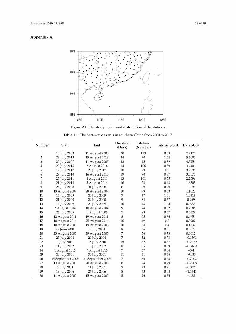
139 stations can be seen from Figure A1 in Appendix A. The ERA5 hourly reanalysis at a resolutionof 0.25◦ × 0.25◦ is the latest reanalysis produced by the European Centre for Medium-Range WeatherForecasts (ECMWF) [19]. The variables of the ERA5 we used in this study include the zonal and meridionalcomponents of wind, geopotential height, 2 m air temperature, and sea surface temperature. The OLR dailymean data used in the study were acquired from the National Oceanic and Atmospheric Administration(NOAA), with a resolution of 2.5◦ × 2.5◦. The ERA5 data were interpolated by mean onto a commonhorizontal resolution: 2.5◦ × 2.5◦. All of these datasets span the 18 years from 2000 to 2017.

2.2. Method to Define Heat-Wave Events

In this study, the definition of heat-wave events basically follows Ding and Qian [18]. The impactsof heat-wave events not only depend on the instantaneous values of air temperature, but the dailymaximum, as well as the duration and area covered. In order to define a compound heat-wave index toconsider all the aforementioned factors, we first rank the daily maximum air temperatures of individualstations (139 in total) in SC from large to small in the 18 years to find out the threshold of the 90thpercentile of each station (use all the daily values of the years). Then, we define an abnormal highair temperature day for each individual station if the daily maximum air temperature of the stationexceeds the threshold of the 90th percentile.

Since the abnormal high air temperature of a given site need to last several days to have significantimpact on human beings [18], the heat-wave events we targeted in this study were required to lastat least one week. To be valid as a heat-wave event, its impact area should cover at least 10 adjacentstations in the same period [18]. The distance between any two stations, i and j, is estimated as:

D =

√[lat(i) − lat(j)]2 + [lon(i) − lon(j)]2, i , j, (1)

where the lat(i) and lon(i) are the ith station’s latitude and longitude. If D ≤ 3, two stations wereconsidered to be adjacent [18].

In summary, when there are more than 10 adjacent stations whose daily maximum air temperatureexceeds its own threshold of 90th percentile and lasts for more than 7 days, this event is defined asa heat-wave event in SC. In addition, in order to facilitate the selection of events, if there is one daywithin the scope of definition that does not meet the requirements, it is determined as the end time ofthe event. In other words, the minimum interval between two events is one day.

2.3. Definition of Heat-Wave Compound Index

In several previous studies, there have been many works about the definition and identification ofheat-wave events for other regions of the world [20–23]. For example, in the work of Stefanon et al. [20],they use a simple definition based on temperature only: a heat-wave event is defined when the temperatureexceeds a given threshold, and they impose additional constraints on the spatial and temporal extensions.Researchers are generally aware that a heat-wave should be measured in terms of duration and extent ofimpact. However, the difference in heat intensity between different heat-wave events is ignored, whichmeans that two events of the same length will be considered as equally severe, even if one of them has ahigher air temperature values than the other. Therefore, there is a need to redefine a heat-wave index,which can account for the duration, impact extent, and intensity of the heat-wave. With such a compoundindex, the selected heat-wave events can be ranked quantitatively, which will facilitate the study of thecontrolling factors and the predictability of the most severe heat-wave events.

For all heat-wave events selected in Section 2.2, an integrated compound index is defined forindividual heat-wave events based on their durations, the numbers of abnormal sites, and the degreesto which the daily maximum air temperature is higher than the threshold of the 90th percentile.The formula used to calculate the compound index of a given heat-wave event is the following:

C(i) = T(i) + A(i) + S(i), (2)

Atmosphere 2020, 11, 668 5 of 19

The C(i) represents the compound index of the ith event. The T(i), A(i), and S(i), respectively, are thestandardized duration index, area index and strength index by using the Z-score standardization [24].The duration index T(i) is obtained by standardizing the duration of the ith event. The longer theevent lasts, the greater the duration index. The area index A(i) reflects the spatial impact of the ithevent, which is calculated by standardizing the number of abnormal stations whose daily maximumair temperature exceeds the threshold of the 90th percentile between the beginning and the end of theevent. The larger the number of abnormal sites during the event, the wider the impact scope of theevent and the larger the value of the area index. In order to avoid events with similar duration indexand area index but larger difference in daily maximum air temperature being mistaken for an event ofthe same degree, the calculation method of the strength index S(i) is as follows: first, calculating thesum of the deviation between the daily maximum air temperature of each station and 35 ◦C for theith event (including several days and stations), then averaging the sum for the number of days andstations, and finally standardizing. The larger the strength index, the stronger is this event.

3. The Objective Identification of the EHW Events

According to the definition of heat-wave events in Section 2.2, all the heat-wave events in SCfrom 2000 to 2017 were selected. During this period, there were 43 heat-wave events occurring in SC.Among these heat-wave events, the durations of some events can be as long as 30 days, the others canbe as short as 7 days. The number of stations with abnormal high air temperature varies between 129and 10. On average, there are 2.4 heat-wave events annually. During this period, each year has at leastone heat-wave event, with a maximum of three events in some years. Among the 43 heat-wave events,there are eight events lasting more than 15 days (including 15 days); the others last less than 15 days.The events lasting more than 15 days occurred once, respectively, in 2003, 2007, 2013, 2014, 2016 and2017, but twice in 2010 (Table A1 in Appendix A).

The compound indices of 43 selected heat-wave events are calculated. Their values vary betweena maximum of 7.22 and a minimum of −4.02. The negative values indicate that the overall intensitiesof these events are below the median strength of all selected events. All events with a compoundindex smaller than one are categorized as normal. In this study, we simply lumped all events withthe compound index larger than one as EHW events. Among all the 43 heat-wave events, there are11 heat-wave events with a compound index greater than 1.0 (Table 1), which will serve as the targetEHW events in this study. Among these top 11 EHW events, there are six events that last longer than15 days and five events that last less than 15 days. Ten of 11 EHW events have their onset days in July.The two most severe EHW events occurred, respectively, in 2003 and 2013. These two ultra-extremecases lasted much longer than 15 days and have drawn much attention and been widely studied asmentioned in introduction [2,3].

Table 1. The top 11 extreme heat-wave (EHW) events in southern China from 2000 to 2017.

Number Start End Duration (Days) Station (Number) Intensity-S(i) Index-C(i)

1 13 July 2003 11 August 2003 30 129 0.89 7.21712 23 July 2013 15 August 2013 24 70 1.54 5.60053 20 July 2007 11 August 2007 23 95 0.89 4.72514 20 July 2016 2 August 2016 14 106 0.89 3.44015 12 July 2017 29 July 2017 18 79 0.9 3.25986 29 July 2010 16 August 2010 19 70 0.87 3.05757 23 July 2011 4 August 2011 13 101 0.55 2.25968 21 July 2014 5 August 2014 16 76 0.43 1.65059 24 July 2008 31 July 2008 8 69 0.99 1.2695

10 19 August 2009 28 August 2009 10 99 0.33 1.102311 14 July 2005 20 July 2005 7 67 1.01 1.0619

Atmosphere 2020, 11, 668 6 of 19

4. The Multi-Scale Controlling Factors of the EHW Events

4.1. Multi-Scale Features Associated with the EHW Events

There have been many previous studies on various aspects of extreme heat-waves [25–30].However, little is known on how variability of different time-scales acts synthetically to producethe most severe extreme heat-wave in SC as identified in the preceding section. To unravel thecontrolling factors of different time-scale variability on the 11 EHW events, the 2 m air temperatureof the year in which the EHW occurred was decomposed into 3–10-day synoptic disturbances,10–30-day, and 30–90-day intra-seasonal variability (ISV) by using the Butterworth band-pass filter [31].For long-term events persisting longer than 15 days (Figure 1), the onsets of the EHW events largelycorrespond to the peaks or negative-to-positive transitions of both the 3–10-day and 10–30-dayvariability, which is consistent with the previous composite results of Chen et al. [5,6]. This resultsuggests that, in addition to synoptic disturbances, the 10–30-day ISV plays an important role in theonsets of long-term EHW events in SC, offering potential predictability on extended-range time-scale.At the same time, robust positive 30–90-day ISV signals exist during the course of the long-termEHW events. The ends of the long-term EHW events largely correspond to the positive-to-negativetransitions of both the 30–90-day and 10–30-day ISV, which is consistent with the previous compositeresults of Chen et al. [5,6]. This result suggests that the persistence of long-term EHW events isdominated by 30–90-day ISV.

Atmosphere 2020, 10, x FOR PEER REVIEW 6 of 19

4. The Multi-Scale Controlling Factors of the EHW Events

4.1. Multi-Scale Features Associated with the EHW Events

There have been many previous studies on various aspects of extreme heat-waves [25–30]. However, little is known on how variability of different time-scales acts synthetically to produce the most severe extreme heat-wave in SC as identified in the preceding section. To unravel the controlling factors of different time-scale variability on the 11 EHW events, the 2 m air temperature of the year in which the EHW occurred was decomposed into 3–10-day synoptic disturbances, 10–30-day, and 30–90-day intra-seasonal variability (ISV) by using the Butterworth band-pass filter [31]. For long-term events persisting longer than 15 days (Figure 1), the onsets of the EHW events largely correspond to the peaks or negative-to-positive transitions of both the 3–10-day and 10–30-day variability, which is consistent with the previous composite results of Chen et al. [5,6]. This result suggests that, in addition to synoptic disturbances, the 10–30-day ISV plays an important role in the onsets of long-term EHW events in SC, offering potential predictability on extended-range time-scale. At the same time, robust positive 30–90-day ISV signals exist during the course of the long-term EHW events. The ends of the long-term EHW events largely correspond to the positive-to-negative transitions of both the 30–90-day and 10–30-day ISV, which is consistent with the previous composite results of Chen et al. [5,6]. This result suggests that the persistence of long-term EHW events is dominated by 30–90-day ISV.

For short-term EHW events less than 15 days (Figure 2), the multi-scale controlling factors are different from that of long-term events. Both the 3–10-day synoptic disturbances and 10–30-day ISV contribute to the onsets and durations with the latter (former) playing a major (minor) role. This finding is also consistent with the composites of Chen et al. [5]. The time scale of 30–90 days does not seem to have much effect on short-term events, whether in the onset or in the duration.

Figure 1. Temporal evolutions of area-mean (25° N–30° N, 113° E–118° E) daily 2 m air temperature (2 m-T) (°C, gray bars) and associated decompositions (Decomp): the climatological annual cycle across 2000–2017, 3-to-10-day synoptic disturbances, 10-to-30-day and 30-to-90-day intra-seasonal variability (the four solid lines in the top panel) along with (bottom panel) the daily compound indices (Cd) for two typical EHW events persisting more than 15 days, respectively, in (a) 2003 and (b) 2007 (Table 1). The time periods of two EHW events are highlighted within two vertical dashed lines in the two top panels of (a,b).

Figure 1. Temporal evolutions of area-mean (25◦ N–30◦ N, 113◦ E–118◦ E) daily 2 m air temperature(2 m-T) (◦C, gray bars) and associated decompositions (Decomp): the climatological annual cycle across2000–2017, 3-to-10-day synoptic disturbances, 10-to-30-day and 30-to-90-day intra-seasonal variability(the four solid lines in the top panel) along with (bottom panel) the daily compound indices (Cd) fortwo typical EHW events persisting more than 15 days, respectively, in (a) 2003 and (b) 2007 (Table 1).The time periods of two EHW events are highlighted within two vertical dashed lines in the two toppanels of (a,b).

For short-term EHW events less than 15 days (Figure 2), the multi-scale controlling factors aredifferent from that of long-term events. Both the 3–10-day synoptic disturbances and 10–30-day ISVcontribute to the onsets and durations with the latter (former) playing a major (minor) role. This findingis also consistent with the composites of Chen et al. [5]. The time scale of 30–90 days does not seem tohave much effect on short-term events, whether in the onset or in the duration.

Atmosphere 2020, 11, 668 7 of 19Atmosphere 2020, 10, x FOR PEER REVIEW 7 of 19

Figure 2. Same as Figure 1, but for two typical EHW events persisting less than 15 days, respectively, in (a) 2016 and (b) 2011.

However, the ISV signals alone could not be used to detect the occurrences of the EHW events because they exist year-around no matter what (Figures 1 and 2). In order to detect the occurrence and track the temporal evolution of an EHW event in SC, a daily compound index was introduced. Unlike the integrated compound index defined in Section 2.3, the EHW daily compound index here only considers the spatial extent and intensity of individual events. Specifically, the daily compound index is defined as:

Cd = Ad + Sd, (3)

where Cd, Ad, and Sd are, respectively, the daily compound index, and its two components: standardized daily area index and strength index. The Ad is the number of all stations with daily maximum air temperature larger than the threshold of the 90th percentile of a station (no need to be adjacent points but within the SC domain), which needs to be standardized with the standard deviation used to standardize the A(i) in Equation (2). Along the same line, Sd is the daily strength index formed by accumulating the differences between the maximum daily air temperature and 35 °C for all stations exceeding the threshold of 90th percentile (if the maximum daily air temperature is below 35 °C, then providing a negative value and the stations in this case do not need to be adjacent), then divided by the number of the stations and standardized by the value used to the S(i) in Equation (2).

The standardized values of Ad and Sd are between −1 and 1. Therefore, the value of the EHW daily compound index fluctuates between −2 and 2. The higher the daily compound index, the greater the heat-wave area and intensity in SC on that day, the more likely an EHW event will occur. By analyzing the daily compound index of the top 11 EHW events, it was found that the probability of EHW events is extremely high when the daily compound index reaches to around 1.2. Figures 1 and 2 indicate that when the daily compound index is greater than 1.2, it corresponds to the onset time of the EHW events in SC. In addition, the EHW daily compound index largely remains greater than 1.2 during the event, eventually dropping rapidly to negative values at the end of the event. Whether it is a long-term event greater than 15 days or a short-term event less than 15 days, the EHW daily compound index serves as a useful indicator for the occurrence and onset time of an EHW event.

EHW events in SC mainly occur in July and August. Although the regionally-averaged 2 m air temperature in July and August is always the highest in a year, during some periods of July and August, it may reach beyond the climatological annual cycle (Figures 1 and 2), these periods do not automatically qualify as EHW events. It should be assessed in combination with other important factors: e.g., the daily compound index, synoptic and intra-seasonal variability. When the daily

Figure 2. Same as Figure 1, but for two typical EHW events persisting less than 15 days, respectively,in (a) 2016 and (b) 2011.

However, the ISV signals alone could not be used to detect the occurrences of the EHW eventsbecause they exist year-around no matter what (Figures 1 and 2). In order to detect the occurrenceand track the temporal evolution of an EHW event in SC, a daily compound index was introduced.Unlike the integrated compound index defined in Section 2.3, the EHW daily compound index hereonly considers the spatial extent and intensity of individual events. Specifically, the daily compoundindex is defined as:

Cd = Ad + Sd, (3)

where Cd, Ad, and Sd are, respectively, the daily compound index, and its two components:standardized daily area index and strength index. The Ad is the number of all stations withdaily maximum air temperature larger than the threshold of the 90th percentile of a station (no needto be adjacent points but within the SC domain), which needs to be standardized with the standarddeviation used to standardize the A(i) in Equation (2). Along the same line, Sd is the daily strengthindex formed by accumulating the differences between the maximum daily air temperature and 35 ◦Cfor all stations exceeding the threshold of 90th percentile (if the maximum daily air temperature is below35 ◦C, then providing a negative value and the stations in this case do not need to be adjacent), thendivided by the number of the stations and standardized by the value used to the S(i) in Equation (2).

The standardized values of Ad and Sd are between−1 and 1. Therefore, the value of the EHW dailycompound index fluctuates between −2 and 2. The higher the daily compound index, the greater theheat-wave area and intensity in SC on that day, the more likely an EHW event will occur. By analyzingthe daily compound index of the top 11 EHW events, it was found that the probability of EHW eventsis extremely high when the daily compound index reaches to around 1.2. Figures 1 and 2 indicate thatwhen the daily compound index is greater than 1.2, it corresponds to the onset time of the EHW eventsin SC. In addition, the EHW daily compound index largely remains greater than 1.2 during the event,eventually dropping rapidly to negative values at the end of the event. Whether it is a long-term eventgreater than 15 days or a short-term event less than 15 days, the EHW daily compound index serves asa useful indicator for the occurrence and onset time of an EHW event.

EHW events in SC mainly occur in July and August. Although the regionally-averaged 2 m airtemperature in July and August is always the highest in a year, during some periods of July andAugust, it may reach beyond the climatological annual cycle (Figures 1 and 2), these periods do notautomatically qualify as EHW events. It should be assessed in combination with other importantfactors: e.g., the daily compound index, synoptic and intra-seasonal variability. When the daily

Atmosphere 2020, 11, 668 8 of 19

compound index reaches about 1.2, the regionally-averaged air temperature is apparently higher thanthe climatological annual cycle, the 3–10-day and 10–30-day variability is peaking or transitioning fromnegative to positive anomaly, the occurrence probability of EHW events in SC is extremely high.

Through decomposition and analysis of the air temperature in SC, it was found that the variabilityof different time scales may have complementary roles on shaping the EHW events. However,what are the precursory signals of the EHW events in SC? How will multi-scale variability actsynthetically to affect the characteristics of the EHW events? The following subsections will bedevoted to addressing these questions. Revealing the precursory signals of the EHW events andunderstanding their controlling factors are essential to the prediction of the EHW events and to mitigatetheir societal-economic impacts.

4.2. Impacts of Intra-Seasonal Variability on the Life-Cycle of the EHW Events

Previous studies with individual cases revealed that anticyclonic circulations associated withanomalous high-pressure systems are the major cause of EHW events [32,33]. Li et al. [14] found thatthe time series of 500 hPa geopotential height anomaly averaged over the middle and lower reachesof the Yangtze River (26.4◦ N~34.2◦ N, 105◦ E~122◦ E) had high positive correlation with the totalheat-wave for all the stations in the region during 1979–2013 summers.

Since the air temperature anomaly in SC is well correlated with the 500 hPa geopotential heightanomaly [2,3], it is interesting to see whether the early signals of EHW events can be found from the500 hPa geopotential height anomaly. As indicated from the temporal analyses (Figures 1 and 2),the EHW events in SC are strongly associated with ISV. We also know that the associated ISV maycome from different sources [34–36]: The westward-propagating ISV from the western Pacific; thenorthward-propagating ISV from the equatorial region. In the following analyses, we make respectivecomposites of surface air temperature and 500 hPa geopotential height anomalies associated with10–30-day and 30–90-day ISV for the short-term only, long-term only, and all top 11 EHW events toexplore how these known ISVs will impact the EHW events.

It was found that, during the onsets of short-term (Figure 3a), long-term (Figure 3b), and all EHW(Figure 3c) events, the composite positive surface air temperature anomalies in SC coincide with thepositive 500 hPa geopotential height anomalies on the 10–30-day time scale. The positive anomalyof short-term events is the strongest (Figure 3a), and the duration of short-term events is basicallycontrolled by the positive anomaly of 500 hPa geopotential height associated with the 10–30-day ISV.It is worth mentioning that for long-term events, 15 days after the onsets of the events, another positiveanomaly of geopotential height reemerges in the study region, which helps maintain the long-termEHW events. For both the short-term and long-term composites (Figure 3a,b), particularly the all-casecomposite (Figure 3c), the positive 500 hPa geopotential height anomalies can be traced back intothe western Pacific. In the composition of all events (Figure 3c), the signal of positive anomaly of500 hPa geopotential height exists more than 15 days before the event onset. The positive anomaly atabout 150◦ W propagates westward all the way to the study area on the EHW onset day. Apparently,westward-propagating 10–30-days ISV from the western Pacific is a potential precursory signal for theEHW events in SC with a lead time of one-to-two weeks [5,6].

The 500 hPa geopotential height anomalies of 30–90-day ISV have little effect on short-term EHWevents (Figure 4a). However, for long-term EHW events, the 500 hPa geopotential height anomaly of30–90-day affects the whole period (Figure 4b). The duration of the long-term EHW event is basicallyoverlapped with the 500 hPa geopotential height positive anomalies of 30–90-day ISV. Averaging allthe EHW events together, the positive anomaly of surface air temperature within the study area isalso co-located with the positive anomaly of 500 hPa geopotential height (Figure 4c). Similar to the10–30-day ISV, the westward-propagating 30–90-day ISV is also a potential precursory signal of theEHW events in SC with a lead time of about one month. In particular, the 30–90-day ISV has a strongeffect on the persistence of long-term events [6].

Atmosphere 2020, 11, 668 9 of 19Atmosphere 2020, 10, x FOR PEER REVIEW 9 of 19

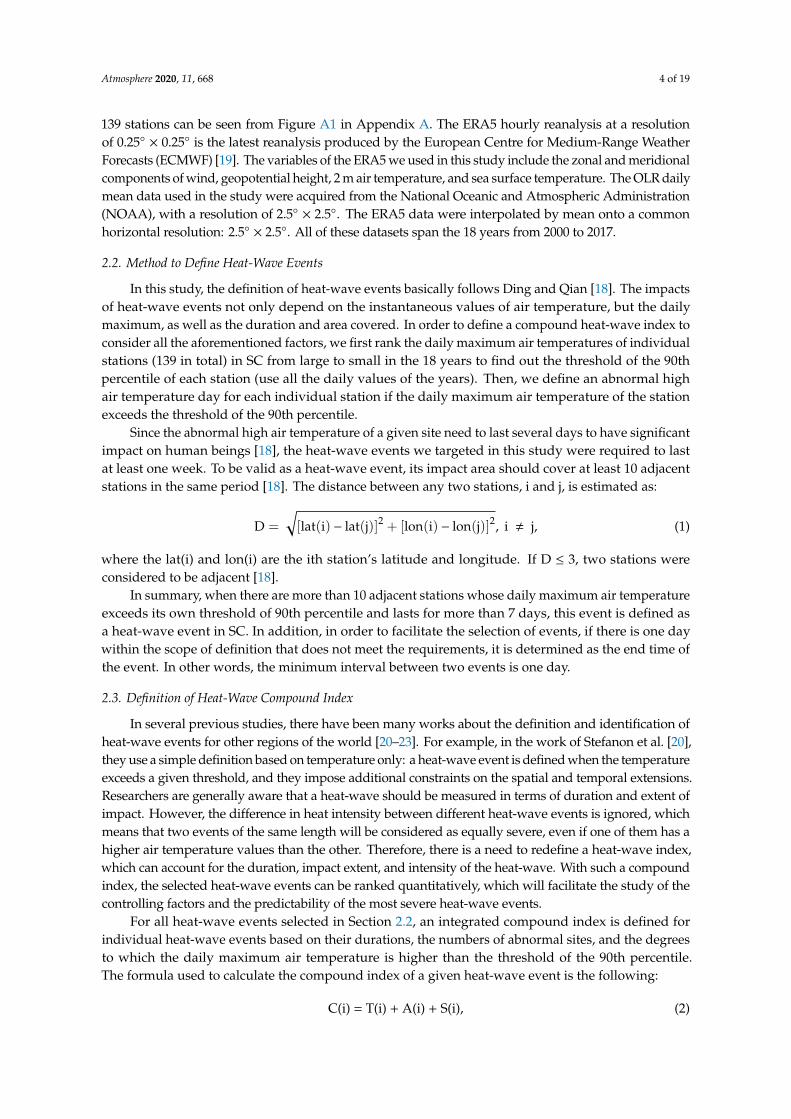
Figure 3. Composite time-longitude sections of 10-to-30-day surface air temperature anomalies {contours (dashed: negative, solid: positive), CI: 0.1 °C} and 500-hPa geopotential height anomalies (shading, unit: dagpm) averaged between 20° N–30° N for the EHW events persisting less than 15 days (a), longer than 15 days (b) and (c) all EHW events. The “lag0day” represents the onset time of individual EHW events over our study area. The domain within two vertical dashed lines highlights our study area.

The 500 hPa geopotential height anomalies of 30–90-day ISV have little effect on short-term EHW events (Figure 4a). However, for long-term EHW events, the 500 hPa geopotential height anomaly of 30–90-day affects the whole period (Figure 4b). The duration of the long-term EHW event is basically overlapped with the 500 hPa geopotential height positive anomalies of 30–90-day ISV. Averaging all the EHW events together, the positive anomaly of surface air temperature within the study area is also co-located with the positive anomaly of 500 hPa geopotential height (Figure 4c). Similar to the 10–30-day ISV, the westward-propagating 30–90-day ISV is also a potential precursory signal of the EHW events in SC with a lead time of about one month. In particular, the 30–90-day ISV has a strong effect on the persistence of long-term events [6].

Figure 4. Same as Figure 3, but for 30-to-90-day intra-seasonal variability with doubled time scales for the ordinate. EHW events persisting less than 15 days (a), longer than 15 days (b) and (c) all EHW events

In order to investigate whether the EHW events have precursory signals in the north–south directions, Figure 5 gives the hovmoller diagrams of the temporal-meridional distribution of the zonal mean surface air temperature and 500 hPa geopotential height anomalies of 10–30-day ISV in SC. For short-term EHW events, the positive anomalies of surface air temperature and 500 hPa geopotential height well match each other during the events (Figure 5a). The initial signal of positive geopotential height anomaly first appears at 20° N about 7 days before the onset. It gradually propagates northward to the study area to initiate the onsets of the EHW events. However, there is no apparent northward-propagating 10–30-day ISV signal in association with the onsets of long-term

Figure 3. Composite time-longitude sections of 10-to-30-day surface air temperature anomalies{contours (dashed: negative, solid: positive), CI: 0.1 ◦C} and 500-hPa geopotential height anomalies(shading, unit: dagpm) averaged between 20◦ N–30◦ N for the EHW events persisting less than 15 days(a), longer than 15 days (b) and (c) all EHW events. The “lag0 day” represents the onset time ofindividual EHW events over our study area. The domain within two vertical dashed lines highlightsour study area.


Figure 3. Composite time-longitude sections of 10-to-30-day surface air temperature anomalies {contours (dashed: negative, solid: positive), CI: 0.1 °C} and 500-hPa geopotential height anomalies (shading, unit: dagpm) averaged between 20° N–30° N for the EHW events persisting less than 15 days (a), longer than 15 days (b) and (c) all EHW events. The “lag0day” represents the onset time of individual EHW events over our study area. The domain within two vertical dashed lines highlights our study area.

The 500 hPa geopotential height anomalies of 30–90-day ISV have little effect on short-term EHW events (Figure 4a). However, for long-term EHW events, the 500 hPa geopotential height anomaly of 30–90-day affects the whole period (Figure 4b). The duration of the long-term EHW event is basically overlapped with the 500 hPa geopotential height positive anomalies of 30–90-day ISV. Averaging all the EHW events together, the positive anomaly of surface air temperature within the study area is also co-located with the positive anomaly of 500 hPa geopotential height (Figure 4c). Similar to the 10–30-day ISV, the westward-propagating 30–90-day ISV is also a potential precursory signal of the EHW events in SC with a lead time of about one month. In particular, the 30–90-day ISV has a strong effect on the persistence of long-term events [6].


In order to investigate whether the EHW events have precursory signals in the north–south directions, Figure 5 gives the hovmoller diagrams of the temporal-meridional distribution of the zonal mean surface air temperature and 500 hPa geopotential height anomalies of 10–30-day ISV in SC. For short-term EHW events, the positive anomalies of surface air temperature and 500 hPa geopotential height well match each other during the events (Figure 5a). The initial signal of positive geopotential height anomaly first appears at 20° N about 7 days before the onset. It gradually propagates northward to the study area to initiate the onsets of the EHW events. However, there is no apparent northward-propagating 10–30-day ISV signal in association with the onsets of long-term

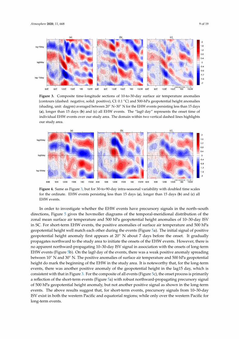
Figure 4. Same as Figure 3, but for 30-to-90-day intra-seasonal variability with doubled time scalesfor the ordinate. EHW events persisting less than 15 days (a), longer than 15 days (b) and (c) allEHW events.

In order to investigate whether the EHW events have precursory signals in the north–southdirections, Figure 5 gives the hovmoller diagrams of the temporal-meridional distribution of thezonal mean surface air temperature and 500 hPa geopotential height anomalies of 10–30-day ISVin SC. For short-term EHW events, the positive anomalies of surface air temperature and 500 hPageopotential height well match each other during the events (Figure 5a). The initial signal of positivegeopotential height anomaly first appears at 20◦ N about 7 days before the onset. It graduallypropagates northward to the study area to initiate the onsets of the EHW events. However, there isno apparent northward-propagating 10–30-day ISV signal in association with the onsets of long-termEHW events (Figure 5b). On the lag0 day of the events, there was a weak positive anomaly spreadingbetween 10◦ N and 30◦ N. The positive anomalies of surface air temperature and 500 hPa geopotentialheight do mark the beginning of the EHW in the study area. It is noteworthy that, for the long-termevents, there was another positive anomaly of the geopotential height in the lag15 day, which isconsistent with that in Figure 3. For the composite of all events (Figure 5c), the onset process is primarilya reflection of the short-term events (Figure 5a) with robust northward-propagating precursory signalof 500 hPa geopotential height anomaly, but not another positive signal as shown in the long-termevents. The above results suggest that, for short-term events, precursory signals from 10–30-dayISV exist in both the western Pacific and equatorial regions; while only over the western Pacific forlong-term events.

Atmosphere 2020, 11, 668 10 of 19


EHW events (Figure 5b). On the lag0 day of the events, there was a weak positive anomaly spreading between 10° N and 30° N. The positive anomalies of surface air temperature and 500 hPa geopotential height do mark the beginning of the EHW in the study area. It is noteworthy that, for the long-term events, there was another positive anomaly of the geopotential height in the lag15 day, which is consistent with that in Figure 3. For the composite of all events (Figure 5c), the onset process is primarily a reflection of the short-term events (Figure 5a) with robust northward-propagating precursory signal of 500 hPa geopotential height anomaly, but not another positive signal as shown in the long-term events. The above results suggest that, for short-term events, precursory signals from 10–30-day ISV exist in both the western Pacific and equatorial regions; while only over the western Pacific for long-term events.

Figure 5. Composite time-latitude sections of 10-to-30-day surface air temperature anomalies {contours (dashed: negative, solid: positive), CI: 0.1 °C} and 500-hPa geopotential height anomalies (shading, unit: dagpm) averaged between 110° E–120° E for the EHW events persisting less than 15 days (a), longer than 15 days (b) and (c) all EHW events. The “lag0day” represents the onset time of individual EHW events over our study area. The domain within two vertical dashed lines highlights our study area.

Figure 6 examines the possible impacts of 30–90-day ISV on the EHW events in SC on the north–south direction. For the short-term events (Figure 6a), no apparent precursory signal exists; but the very weak positive anomaly of the 500 hPa geopotential height associated with the EHW events is significantly amplified on the way towards the middle and lower reaches of the Yangtze River. For the long-term events (Figure 6b), robust positive anomaly of geopotential height appears a few days before the onset, co-existing with the EHW events for more than 15 days, then propagating further north to impact the middle and lower reaches of the Yangtze River. The composite of all events (Figure 6c) also shows a moderate signal over the study region with amplified impact northward.

Figure 5. Composite time-latitude sections of 10-to-30-day surface air temperature anomalies {contours(dashed: negative, solid: positive), CI: 0.1 ◦C} and 500-hPa geopotential height anomalies (shading, unit:dagpm) averaged between 110◦ E–120◦ E for the EHW events persisting less than 15 days (a), longerthan 15 days (b) and (c) all EHW events. The “lag0 day” represents the onset time of individual EHWevents over our study area. The domain within two vertical dashed lines highlights our study area.

Figure 6 examines the possible impacts of 30–90-day ISV on the EHW events in SC on thenorth–south direction. For the short-term events (Figure 6a), no apparent precursory signal exists;but the very weak positive anomaly of the 500 hPa geopotential height associated with the EHWevents is significantly amplified on the way towards the middle and lower reaches of the YangtzeRiver. For the long-term events (Figure 6b), robust positive anomaly of geopotential height appears afew days before the onset, co-existing with the EHW events for more than 15 days, then propagatingfurther north to impact the middle and lower reaches of the Yangtze River. The composite of all events(Figure 6c) also shows a moderate signal over the study region with amplified impact northward.


EHW events (Figure 5b). On the lag0 day of the events, there was a weak positive anomaly spreading between 10° N and 30° N. The positive anomalies of surface air temperature and 500 hPa geopotential height do mark the beginning of the EHW in the study area. It is noteworthy that, for the long-term events, there was another positive anomaly of the geopotential height in the lag15 day, which is consistent with that in Figure 3. For the composite of all events (Figure 5c), the onset process is primarily a reflection of the short-term events (Figure 5a) with robust northward-propagating precursory signal of 500 hPa geopotential height anomaly, but not another positive signal as shown in the long-term events. The above results suggest that, for short-term events, precursory signals from 10–30-day ISV exist in both the western Pacific and equatorial regions; while only over the western Pacific for long-term events.

Figure 5. Composite time-latitude sections of 10-to-30-day surface air temperature anomalies {contours (dashed: negative, solid: positive), CI: 0.1 °C} and 500-hPa geopotential height anomalies (shading, unit: dagpm) averaged between 110° E–120° E for the EHW events persisting less than 15 days (a), longer than 15 days (b) and (c) all EHW events. The “lag0day” represents the onset time of individual EHW events over our study area. The domain within two vertical dashed lines highlights our study area.

Figure 6 examines the possible impacts of 30–90-day ISV on the EHW events in SC on the north–south direction. For the short-term events (Figure 6a), no apparent precursory signal exists; but the very weak positive anomaly of the 500 hPa geopotential height associated with the EHW events is significantly amplified on the way towards the middle and lower reaches of the Yangtze River. For the long-term events (Figure 6b), robust positive anomaly of geopotential height appears a few days before the onset, co-existing with the EHW events for more than 15 days, then propagating further north to impact the middle and lower reaches of the Yangtze River. The composite of all events (Figure 6c) also shows a moderate signal over the study region with amplified impact northward.

Figure 6. Same as Figure 5, but for 30-to-90-day intra-seasonal variability with doubled time scalesfor the ordinate. EHW events persisting less than 15 days (a), longer than 15 days (b) and (c) allEHW events.

In the above analyses, we revealed that westward (northward)-propagating ISV from the westernPacific (equatorial region) plays a dominant (supportive) role in the occurrences of EHW events in SC.To what degree are these ISV signals connected with the eastward-propagating tropical planetary-scaleMadden–Julian Oscillation [37]? Figure 7a,b shows the along-equatorial composite hovmoller diagramsof OLR and (200 hPa–850 hPa) velocity potential anomalies in association, respectively, with 10–30-dayand 30–90-day ISVs averaged between 30◦ S and 30◦ N. On the 10–30-day time scale (Figure 7a),the onset period of the composite EHW events corresponds to the positive anomalies of OLR and(200 hPa–850 hPa) velocity potential. The action centers shift to the east of the SC, suggesting a strongconnection with the western Pacific subtropical high. The strong subsidence in association with positiveOLR and velocity potential anomalies favors clear sky and the formation of an extended heat-wavein SC. It is worth pointing out that the positive 10–30-day ISV signals affecting the SC in Figure 7a

Atmosphere 2020, 11, 668 11 of 19

are mostly stationary, not resulting from any eastward-propagating precursor on this time scale.This may be connected with the suppressed phase of the 30–90-day MJO before the onset (Figure 7b)through the emanating westward (Figure 3)- and northward (Figure 5)-propagating intraseasonaldisturbances [35,38].



In the above analyses, we revealed that westward (northward)-propagating ISV from the western Pacific (equatorial region) plays a dominant (supportive) role in the occurrences of EHW events in SC. To what degree are these ISV signals connected with the eastward-propagating tropical planetary-scale Madden–Julian Oscillation [37]? Figure 7a,b shows the along-equatorial composite hovmoller diagrams of OLR and (200 hPa-850 hPa) velocity potential anomalies in association, respectively, with 10–30-day and 30–90-day ISVs averaged between 30° S and 30° N. On the 10– 30-day time scale (Figure 7a), the onset period of the composite EHW events corresponds to the positive anomalies of OLR and (200 hPa–850 hPa) velocity potential. The action centers shift to the east of the SC, suggesting a strong connection with the western Pacific subtropical high. The strong subsidence in association with positive OLR and velocity potential anomalies favors clear sky and the formation of an extended heat-wave in SC. It is worth pointing out that the positive 10–30-day ISV signals affecting the SC in Figure 7a are mostly stationary, not resulting from any eastward-propagating precursor on this time scale. This may be connected with the suppressed phase of the 30–90-day MJO before the onset (Figure 7b) through the emanating westward (Figure 3)- and northward (Figure 5)-propagating intraseasonal disturbances [35,38].

There are robust eastward-propagating MJO signals in association with the EHW events in SC (Figure 7b). Two suppressed periods of MJO appear, respectively, before and after the onsets of the EHW events. Therefore, the direct contribution of MJO on EHW events in SC is not for initiation but for their maintenance in particular for the long-term events. At the same time, the 30–90-day MJO may also influence the EHW events in SC, indirectly, through emanating westward (Figure 4)- and northward (Figure 6)-propagating ISV disturbances, respectively, from the western Pacific and equatorial region [35,38].

Figure 7. Composite time-longitude sections of outgoing long-wave radiation (OLR) anomalies {contours (dashed: negative, solid: positive), CI: 1 W m } and (200 hPa–850 hPa) velocity potential anomalies (shading, 10 m s ) of all EHW events averaged between 30° S–30° N in association with (a) 10-to-30-day and (b) 30-to-90-day intra-seasonal variability. The “lag0day” represents the start time of individual EHW events over our target area. The domain within two vertical dashed lines highlights our target area.

To further reveal the possible connections among different ISV components and their impacts on the EHW events in SC, the composite spatial-temporal evolutions of OLR, (200 hPa–850 hPa) velocity potential, and divergent wind anomalies are given in Figures 8 and 9, respectively, for 10–30-day and 30–90-day ISV. On 10–30-day time scale, at about 12 days before the EHW (Figure 8a), there is a positive anomalous center of OLR and velocity potential in the western equatorial Pacific

Figure 7. Composite time-longitude sections of outgoing long-wave radiation (OLR) anomalies{contours (dashed: negative, solid: positive), CI: 1 W m−2} and (200 hPa–850 hPa) velocity potentialanomalies (shading, 106 m2 s−1) of all EHW events averaged between 30◦ S–30◦ N in association with(a) 10-to-30-day and (b) 30-to-90-day intra-seasonal variability. The “lag0 day” represents the start timeof individual EHW events over our target area. The domain within two vertical dashed lines highlightsour target area.

There are robust eastward-propagating MJO signals in association with the EHW events in SC(Figure 7b). Two suppressed periods of MJO appear, respectively, before and after the onsets of theEHW events. Therefore, the direct contribution of MJO on EHW events in SC is not for initiationbut for their maintenance in particular for the long-term events. At the same time, the 30–90-dayMJO may also influence the EHW events in SC, indirectly, through emanating westward (Figure 4)-and northward (Figure 6)-propagating ISV disturbances, respectively, from the western Pacific andequatorial region [35,38].

To further reveal the possible connections among different ISV components and their impacts onthe EHW events in SC, the composite spatial-temporal evolutions of OLR, (200 hPa–850 hPa) velocitypotential, and divergent wind anomalies are given in Figures 8 and 9, respectively, for 10–30-day and30–90-day ISV. On 10–30-day time scale, at about 12 days before the EHW (Figure 8a), there is a positiveanomalous center of OLR and velocity potential in the western equatorial Pacific near the island ofNew Guinea, which may be an emanated 10–30-day ISV disturbance from the eastward-propagatingMJO suppressed phase (Figures 7 and 9a). At the same time, a negative OLR anomalous belt presentsat the northwest of the positive OLR anomalous center, extending from the eastern equatorial IndianOcean to the east of the Philippines with negative anomalies of potential velocity over a broaderregion. Consistent with Figure 3c, the positive anomalies in the western equatorial Pacific propagatenorthwestward in the following days (Figure 8b,c). About 3-days before the EHW onset (Figure 8d),the positive OLR and velocity potential anomalous center reaches 15◦ N around the Philippines and aresignificantly amplified by strong easterly shear of the Asian summer monsoon [39]. At the onset dayof the EHW (Figure 8e), SC is in the center of positive anomalies of velocity potential and OLR, as wellas the strong convergence of upper-level winds. Therefore, SC is controlled by subsidence. On thethird day after the onset of the EHW events (Figure 8f), the positive anomalies of the 10–30-day ISVbegin to weaken gradually. On the lag6 days (Figure 8g), the SC is already covered with the negativevelocity potential and OLR anomalies.

Atmosphere 2020, 11, 668 12 of 19


near the island of New Guinea, which may be an emanated 10–30-day ISV disturbance from the eastward-propagating MJO suppressed phase (Figures 7 and 9a). At the same time, a negative OLR anomalous belt presents at the northwest of the positive OLR anomalous center, extending from the eastern equatorial Indian Ocean to the east of the Philippines with negative anomalies of potential velocity over a broader region. Consistent with Figure 3c, the positive anomalies in the western equatorial Pacific propagate northwestward in the following days (Figure 8b,c). About 3-days before the EHW onset (Figure 8d), the positive OLR and velocity potential anomalous center reaches 15° N around the Philippines and are significantly amplified by strong easterly shear of the Asian summer monsoon [39]. At the onset day of the EHW (Figure 8e), SC is in the center of positive anomalies of velocity potential and OLR, as well as the strong convergence of upper-level winds. Therefore, SC is controlled by subsidence. On the third day after the onset of the EHW events (Figure 8f), the positive anomalies of the 10–30-day ISV begin to weaken gradually. On the lag6 days (Figure 8g), the SC is already covered with the negative velocity potential and OLR anomalies.

Figure 8. Composite horizontal spatial-temporal evolutions of 10-to-30-day OLR anomalies (shading, W ) and (200 hPa–850 hPa) velocity potential anomalies {contours (dashed: negative, solid: positive), CI: 0.5 10 } along with (200 hPa–850 hPa) divergent wind anomalies (vectors, ) of all EHW events on lag days of −12 (a), −9 (b), −6 (c), −3 (d), 0 (e), 3 (f), 6 (g), 9 (h).

Figure 8. Composite horizontal spatial-temporal evolutions of 10-to-30-day OLR anomalies (shading,W m−2) and (200 hPa–850 hPa) velocity potential anomalies {contours (dashed: negative, solid: positive),CI: 0.5 106 m2 s−1} along with (200 hPa–850 hPa) divergent wind anomalies (vectors, m s−1) of all EHWevents on lag days of −12 (a), −9 (b), −6 (c), −3 (d), 0 (e), 3 (f), 6 (g), 9 (h).

For 30–90-day ISV (Figure 9), the associated velocity potential anomalies exhibitplanetary-scale eastward propagation as has been shown in many previous studies [40–42].Along with the eastward-propagating planetary-scale velocity potential anomalies, the alternativeconvective-and-suppressed phases move northeastward to modulate the evolutions of the Asiansummer monsoon [13,14]. At about 10 days before the EHW onsets, the positive OLR and velocitypotential anomalies in association with previous suppressed phase (Figure 7b), although very weak,have reached the SC (Figure 9a). As the negative velocity potential anomalies move eastward,the positive OLR anomalies persist over the SC until lag10 days (Figure 9b–e), significantly contributingto the onset and persistence of the EHW events [13,14]. In next two pentads (Figure 9f,g), the secondsuppressed phase of the 30–90-day ISV (Figure 7b) has propagated from the tropical Indian Ocean todirectly affect the Asian continent, including the SC, which also contributes to the persistence of theEHW events.

Atmosphere 2020, 11, 668 13 of 19


For 30–90-day ISV (Figure 9), the associated velocity potential anomalies exhibit planetary-scale eastward propagation as has been shown in many previous studies [40–42]. Along with the eastward-propagating planetary-scale velocity potential anomalies, the alternative convective-and-suppressed phases move northeastward to modulate the evolutions of the Asian summer monsoon [13,14]. At about 10 days before the EHW onsets, the positive OLR and velocity potential anomalies in association with previous suppressed phase (Figure 7b), although very weak, have reached the SC (Figure 9a). As the negative velocity potential anomalies move eastward, the positive OLR anomalies persist over the SC until lag10 days (Figure 9b–e), significantly contributing to the onset and persistence of the EHW events [13,14]. In next two pentads (Figure 9f,g), the second suppressed phase of the 30–90-day ISV (Figure 7b) has propagated from the tropical Indian Ocean to directly affect the Asian continent, including the SC, which also contributes to the persistence of the EHW events.

Figure 9. Same as Figure 8, but for 30-to-90-day intra-seasonal variability on lag days of −10 (a), −5 (b), 0 (c), 5 (d), 10 (e), 15 (f), 20 (g), 25 (h) of all EHW events.

4.3. Why Some Specific Years Are Favored for the Occurrences of the EHW Events?

Figure 10 shows the evolutions of domain-mean daily geopotential height anomalies over SC from 2000 to 2017 in July and August. It can be seen that the long-term EHW events correspond well with the positive anomalies of geopotential height. As can be seen from the right panel of Figure 10,

Figure 9. Same as Figure 8, but for 30-to-90-day intra-seasonal variability on lag days of −10 (a), −5 (b),0 (c), 5 (d), 10 (e), 15 (f), 20 (g), 25 (h) of all EHW events.

4.3. Why Some Specific Years Are Favored for the Occurrences of the EHW Events?

Figure 10 shows the evolutions of domain-mean daily geopotential height anomalies over SCfrom 2000 to 2017 in July and August. It can be seen that the long-term EHW events correspond wellwith the positive anomalies of geopotential height. As can be seen from the right panel of Figure 10,the peak values of the standardized domain-mean air temperature of July and August in SC from 2000to 2017 are well correlated to the years with long-term EHW events. The high correlation betweenthe occurrences of long-term EHW events and regional inter-annual variability of air temperatureand geopotential height motivated us to search for possible remote impact factors. After checking theglobal SSTA in the preceding 12 months of all 11 EHW events, we noticed that key common features arethe positive SSTA over the western North Pacific in summer and the equatorial eastern Pacific in thepreceding winter. For some EHW events, there is also precursory positive SSTA over the Indian Ocean.These findings are largely consistent with Deng et al. [7]. Based on these results, we defined a yearlySSTA index for 18 years from 2000 to 2017. The index standardizes the addition of the mean SSTA ofthe western North Pacific (averaged over 10◦ N–30◦ N, 120◦ E–140◦ E) in May and June as well as thatof the eastern Pacific (averaged over 5◦ S–5◦ N, 130◦ W–170◦ W) in the preceding winter (December,January and February). From Figure 10, it can be seen that all the long-term EHW events occur in theyears with the SSTA index greater than zero. Therefore, on the interannual time scale, the SSTA index

Atmosphere 2020, 11, 668 14 of 19

defined here can serve as a potential seasonal predictor for the occurrences of long-term EHW eventsin a peak summer of SC. The underlying physical processes connecting the SSTA variability to theEHW events deserve further research, which is beyond the scope of the present study.


the peak values of the standardized domain-mean air temperature of July and August in SC from 2000 to 2017 are well correlated to the years with long-term EHW events. The high correlation between the occurrences of long-term EHW events and regional inter-annual variability of air temperature and geopotential height motivated us to search for possible remote impact factors. After checking the global SSTA in the preceding 12 months of all 11 EHW events, we noticed that key common features are the positive SSTA over the western North Pacific in summer and the equatorial eastern Pacific in the preceding winter. For some EHW events, there is also precursory positive SSTA over the Indian Ocean. These findings are largely consistent with Deng et al. [7]. Based on these results, we defined a yearly SSTA index for 18 years from 2000 to 2017. The index standardizes the addition of the mean SSTA of the western North Pacific (averaged over 10° N–30° N, 120° E–140° E) in May and June as well as that of the eastern Pacific (averaged over 5° S–5° N, 130° W–170° W) in the preceding winter (December, January and February). From Figure 10, it can be seen that all the long-term EHW events occur in the years with the SSTA index greater than zero. Therefore, on the interannual time scale, the SSTA index defined here can serve as a potential seasonal predictor for the occurrences of long-term EHW events in a peak summer of SC. The underlying physical processes connecting the SSTA variability to the EHW events deserve further research, which is beyond the scope of the present study.

Figure 10. Temporal evolutions (left part) of domain-averaged (25° N–30° N, 115° E–125° E) daily 500 hPa geopotential height anomalies in two peak summer months (July and August) from 2000 to 2017 (shading, dagpm); the horizontal black solid (dashed) lines, respectively, highlight 11 EHW events persisting longer (shorter) than 15 days. The two zig-zag lines on the right side are, respectively, standardized domain-mean (25° N–30° N, 115° E–125° E) surface air temperature anomalies (SATA) averaged through July and August (in red color) and the associated index of the sea surface temperature anomaly (SSTA) (in blue color, the detail definition of this SSTA index can be found in the context).

5. Concluding Remarks and Discussion

Figure 10. Temporal evolutions (left part) of domain-averaged (25◦ N–30◦ N, 115◦ E–125◦ E) daily500 hPa geopotential height anomalies in two peak summer months (July and August) from 2000to 2017 (shading, dagpm); the horizontal black solid (dashed) lines, respectively, highlight 11 EHWevents persisting longer (shorter) than 15 days. The two zig-zag lines on the right side are, respectively,standardized domain-mean (25◦ N–30◦ N, 115◦ E–125◦ E) surface air temperature anomalies (SATA)averaged through July and August (in red color) and the associated index of the sea surface temperatureanomaly (SSTA) (in blue color, the detail definition of this SSTA index can be found in the context).

5. Concluding Remarks and Discussion

In this study, we described a new method to identify a heat-wave in SC, and then selected43 heat-wave events in 2000–2017. Based on the impact area, duration, and strength of heat-waveevents, a compound index of heat-waves was defined to quantify the overall intensity of heat-waveevents in SC. The top 11 heat-wave events with the compound index greater than one were selected tostudy the multi-scale controlling factors of the EHW in SC. The 2 m air temperature, 500 hPa geopotentialheight, OLR, velocity potential anomalies and associated decompositions (annual cycle, 3–10-daysynoptic disturbances, 10-to-30-day and 30-to-90-day ISV) were analyzed to reveal the multi-scalespatial-temporal variations shaping the EHW events. This pilot study provides a multi-scale perspectivefor further studies of the EHW events in China. The major findings of our study are summarized inthe following:

(1) A daily compound index of heat-waves that combines the spatial extent and strength ofthe heat-wave was established to track the outbreak of the EHW events in SC. The higher the dailycompound index, the greater the heat-wave area and intensity in SC on that day. The probability

Atmosphere 2020, 11, 668 15 of 19

of EHW events is extremely high when the daily compound index reaches around 1.2. This dailycompound index serves as a useful indicator for the occurrence and onset time of an EHW event.

(2) The synoptic variability and 10–30-day ISV induce the onsets of the EHW events in SC;the 30–90-day ISV is the key to the persistence of the EHW events [5,6]. About 12 days before the onsetof the EHW in SC, the 10–30-day positive anomalies of velocity potential and OLR appear near theequatorial western Pacific, which then propagate northwestward. At the same time, the 30–90-daysuppressed phase propagates northeastward from the Indian Ocean to the South China sector [13,14] toinfluence the development of the EHW events. The occurrence of the EHW in SC is coincident with thearrivals of 10–30-day and 30–90-day intra-seasonal signals (e.g., the anomalies of 500 hPa geopotentialheight and OLR) propagating from the east and south. Therefore, monitoring these precursory ISVsignals and the daily compound index together can offer an expert early-warning system of the EHWevents in SC on the extended-range time scale.

(3) On the interannual time scale, it was found that all long-term EHW events in SC occurredin the years with robust warming of the western North Pacific in early summer and warming of theequatorial eastern Pacific in the preceding winter [7]. An interannual SSTA index, which adds the SSTAover the above two regions together, could serve as a useful seasonal predictor of the EHW occurrencein SC at least one-month ahead. The underlying physical processes need further investigations.

These findings enrich our understanding of the objective identification and multi-scale controllingfactors of the EHW events in SC. Further in-depth studies and numerical experiments are neededto reveal and quantify the respective roles of multi-scale processes in shaping individual EHWevents. Empirical models based on our findings can be developed to quantitatively assess theforecasting capability of the EHW events in SC and to compare with the performances of state-of-artsubseasonal-to-seasonal prediction models [43–45].

Under the impacts of global warming, EHW events are expected to further increase in Chinaand around the world. The understanding of the processes driving the regional features of the EHWevents under a changing climate has drawn much attention around the world [46–51]. It has beenrecognized that changes in regional circulation patterns may affect long-term variations of EHW oversome regions [52]. In order to predict future EHW changes more reliably on a regional scale, it isnecessary for models to reliably capture regional circulation changes and their relationship with surfaceair temperature. Since the territory of China covers vast longitudinal and latitudinal ranges withdiverse weather and climate regimes, the major modes that affect extremes in different regions can bevery different. Some previous studies have found that the EHW in specific regions can result fromvarious types of circulation anomalies [53–55]. Even the key circulations affecting nearby sites could bequite different [56]. The bottom-up approach used in this study is a viable method that can be adoptedto other regions to reveal the multi-scale factors in shaping regional EHW events and to developmulti-scale synthetic expert systems for the subseasonal-to-seasonal monitoring and prediction ofregional EHW events.

Author Contributions: J.-X.F. and W.C. conceived and designed the study; W.C. analyzed the data and discussedthe results with J.-X.F. and G.L.; W.C. and J.-X.F. wrote the paper. All authors have read and agreed to the publishedversion of the manuscript.

Funding: This work was jointly supported by the startup fund of Fudan University, the China National ScienceFoundation under grant 41875064 and National Key Research Program and Development of China undergrant 2017YFC1502302.

Acknowledgments: We heartily express our appreciation to the three reviewers for their insightful comments andsuggestions, which helped to improve the manuscript significantly. We also would like to express our gratitude tothe staff of the ECWMF for the ERA5. Without their diligent work, it would have been impossible for us to finishour study and this paper.

Conflicts of Interest: The authors declare no conflict of interest.

Atmosphere 2020, 11, 668 16 of 19

Appendix A


Author Contributions: J.-X.F. and W.C. conceived and designed the study; W.C. analyzed the data and discussed the results with J.-X.F. and G.L.; W.C. and J.-X.F. wrote the paper.

Funding: This work was jointly supported by the startup fund of Fudan University, the China National Science Foundation under grant 41875064 and National Key Research Program and Development of China under grant 2017YFC1502302.

Acknowledgments: We heartily express our appreciation to the three reviewers for their insightful comments and suggestions, which helped to improve the manuscript significantly. We also would like to express our gratitude to the staff of the ECWMF for the ERA5. Without their diligent work, it would have been impossible for us to finish our study and this paper.

Conflicts of Interest: The authors declare no conflict of interest.

Appendix A

Figure A1. The study region and distribution of the stations.

Table A1. The heat-wave events in southern China from 2000 to 2017.

Number Start End Duration

(Days) Station

(Number) Intensity-

S(i) Index-

C(i) 1 2003/7/13 2003/8/11 30 129 0.89 7.2171 2 2013/7/23 2013/8/15 24 70 1.54 5.6005 3 2007/7/20 2007/8/11 23 95 0.89 4.7251 4 2016/7/20 2016/8/2 14 106 0.89 3.4401 5 2017/7/12 2017/7/29 18 79 0.9 3.2598 6 2010/7/29 2010/8/16 19 70 0.87 3.0575 7 2011/7/23 2011/8/4 13 101 0.55 2.2596 8 2014/7/21 2014/8/5 16 76 0.43 1.6505 9 2008/7/24 2008/7/31 8 69 0.99 1.2695

10 2009/8/19 2009/8/28 10 99 0.33 1.1023 11 2005/7/14 2005/7/20 7 67 1.01 1.0619 12 2000/7/21 2000/7/29 9 84 0.57 0.969 13 2009/7/14 2009/7/23 10 45 1.03 0.8954 14 2004/8/2 2004/8/10 9 74 0.62 0.7388 15 2005/7/26 2005/8/1 7 83 0.57 0.5626 16 2011/8/12 2011/8/19 8 55 0.86 0.4651 17 2016/8/10 2016/8/25 16 49 0.3 0.3902 18 2006/8/10 2006/8/19 10 68 0.4 0.1837

Figure A1. The study region and distribution of the stations.

Table A1. The heat-wave events in southern China from 2000 to 2017.

Number Start End Duration(Days)

Station(Number) Intensity-S(i) Index-C(i)

1 13 July 2003 11 August 2003 30 129 0.89 7.21712 23 July 2013 15 August 2013 24 70 1.54 5.60053 20 July 2007 11 August 2007 23 95 0.89 4.72514 20 July 2016 2 August 2016 14 106 0.89 3.44015 12 July 2017 29 July 2017 18 79 0.9 3.25986 29 July 2010 16 August 2010 19 70 0.87 3.05757 23 July 2011 4 August 2011 13 101 0.55 2.25968 21 July 2014 5 August 2014 16 76 0.43 1.65059 24 July 2008 31 July 2008 8 69 0.99 1.269510 19 August 2009 28 August 2009 10 99 0.33 1.102311 14 July 2005 20 July 2005 7 67 1.01 1.061912 21 July 2000 29 July 2000 9 84 0.57 0.96913 14 July 2009 23 July 2009 10 45 1.03 0.895414 2 August 2004 10 August 2004 9 74 0.62 0.738815 26 July 2005 1 August 2005 7 83 0.57 0.562616 12 August 2011 19 August 2011 8 55 0.86 0.465117 10 August 2016 25 August 2016 16 49 0.3 0.390218 10 August 2006 19 August 2006 10 68 0.4 0.183719 26 June 2004 3 July 2004 8 66 0.51 0.007420 23 August 2003 29 August 2003 7 56 0.73 0.001221 23 July 2004 29 July 2004 7 52 0.73 −0.139122 1 July 2010 15 July 2010 15 32 0.37 −0.222923 11 July 2002 18 July 2002 8 65 0.39 −0.316924 1 August 2015 7 August 2015 7 37 0.84 −0.425 20 July 2001 30 July 2001 11 41 0.46 −0.43326 15 September 2005 21 September 2005 7 36 0.73 −0.700227 13 August 2008 20 August 2008 8 24 0.79 −0.790828 3 July 2001 11 July 2001 9 23 0.71 −0.833129 19 July 2006 26 July 2006 8 63 0.08 −1.134130 11 August 2005 15 August 2005 5 26 0.76 −1.35

Atmosphere 2020, 11, 668 17 of 19

Table A1. Cont.

Number Start End Duration(Days)

Station(Number) Intensity-S(i) Index-C(i)

31 27 June 2015 3 July 2015 7 24 0.62 −1.386232 2 September 2009 9 September 2009 8 53 0.09 −1.460833 14 August 2017 21 August 2017 8 36 0.32 −1.502734 10 July 2015 16 July 2015 7 37 0.31 −1.677435 15 September 2010 21 September 2010 7 32 0.17 −2.190236 22 August 2011 29 August 2011 8 11 0.35 −2.307237 15 September 2008 23 September 2008 9 26 −0.05 −2.559538 20 August 2001 25 August 2001 6 30 0.12 −2.566539 22 June 2016 28 June 2016 7 30 0.02 −2.621840 22 July 2012 28 July 2012 7 10 0.14 −3.034141 4 September 2003 10 September 2003 7 11 −0.07 −3.505142 23 August 2002 31 August 2002 9 27 −0.54 −3.705443 11 August 2012 18 August 2012 8 24 −0.55 −4.0203

References

1. World Meteorological Organization (WMO). Seamless Prediction of the Earth System: From Minutes to Months;WMO-No1156; WMO: Geneva, Switzerland, 2015.

2. Ding, T.; Qian, W.H. Statistical characteristics of heat wave precursors in China and model prediction. Chin. J.Geophys. 2012, 55, 1472–1486. (In Chinese)

3. Tang, T.; Jin, R.H.; Peng, X.Y.; Niu, R.Y. The analysis of causes about extremely high temperature in thesummer of 2013 year in the southern region. J. Chengdu Univ. Inf. Technol. 2014, 29, 652–659. (In Chinese)

4. Wang, W.W.; Zhou, W.; Wang, X.; Fong, S.K.; Leong, K.C. Summer high temperature extremes in SoutheastChina associated with the East Asian jet stream and circumglobal teleconnection. J. Geophys. Res. Atmos.2013, 118, 8306–8319. [CrossRef]

5. Chen, R.D.; Wen, Z.P.; Lu, R.Y. Evolutions of the circulation anomalies and the quasi-biweekly oscillationsassociated with extreme heat events in South China. J. Clim. 2016, 19, 6909–6921. [CrossRef]

6. Chen, R.D.; Wen, Z.P.; Lu, R.Y. Large-scale circulation anomalies and intraseasonal oscillations associatedwith long-lived extreme heat events in South China. J. Clim. 2018, 31, 213–232. [CrossRef]

7. Deng, K.Q.; Yang, S.; Ting, M.F.; Zhao, P.; Wang, Z.Y. Dominant modes of China summer heat waves driven byglobal sea surface temperature and atmospheric internal variability. J. Clim. 2019, 32, 3761–3775. [CrossRef]

8. Li, J.; Ding, T.; Jia, X.L.; Zhao, X.C. Analysis on the extreme heat wave over China around Yangtze Riverregion in the summer of 2013 and its main contributing factors. Adv. Meteorol. 2015, 2015, 1–15. [CrossRef]

9. Wang, W.W.; Zhou, W.; Liu, X.Z.; Wang, X.; Wang, D.X. Synoptic-scale characteristics and atmosphericcontrols of summer heat waves in China. Clim. Dyn. 2016, 46, 2923–2941. [CrossRef]

10. Chen, S.Y.; Wang, J.S.; Guo, J.T.; Lu, X.D. Evolution characteristics of the extreme high temperature event inNorthwest China from 1961 to 2009. J. Nat. Res. 2012, 27, 832–844. (In Chinese)

11. Loikith, P.C.; Broccoli, A.J. Characteristics of observed atmospheric circulation patterns associated withtemperature extremes over North America. J. Clim. 2012, 25, 7266–7281. [CrossRef]

12. Gao, M.N.; Yang, J.; Wang, B.; Zhou, S.Y.; Gong, D.Y.; Kim, S.J. How are heat waves over Yangtze River valleyassociated with atmospheric quasi-biweekly oscillation? Clim. Dyn. 2018, 51, 4421–4437. [CrossRef]

13. Diao, Y.F.; Li, T.; Hsu, P.C. Influence of the boreal summer intraseasonal oscillation on extreme temperatureevents in the northern hemisphere. J. Meteorol. Res. 2018, 32, 534–547. [CrossRef]

14. Chen, Y.; Zhai, P.M. Simultaneous modulations of precipitation and temperature extremes in Southern partsof China by the boreal summer intraseasonal oscillation. Clim. Dyn. 2017, 49, 3363–3381. [CrossRef]

15. Ding, T.; Qian, W.H.; Yan, Z.W. Changes in hot days and heat waves in China during 1961–2007. Int. J.Climatol. 2010, 30, 1452–1462. [CrossRef]

16. Chen, R.D.; Wen, Z.P.; Lu, R.Y. Interdecadal change on the relationship between the mid-summer temperaturein South China and atmospheric circulation and sea surface temperature. Clim. Dyn. 2018, 51, 2113–2126.[CrossRef]

http://dx.doi.org/10.1002/jgrd.50633

http://dx.doi.org/10.1175/JCLI-D-16-0160.1



http://dx.doi.org/10.1155/2015/706713

http://dx.doi.org/10.1007/s00382-015-2741-8


http://dx.doi.org/10.1007/s00382-017-3526-z

http://dx.doi.org/10.1007/s13351-018-8031-8

http://dx.doi.org/10.1007/s00382-016-3518-4

http://dx.doi.org/10.1002/joc.1989

http://dx.doi.org/10.1007/s00382-017-4002-5

Atmosphere 2020, 11, 668 18 of 19

17. Song, L.; Wu, R.G.; Jiao, Y. Relative contributions of synoptic and intraseasonal variations to strong coldevents over eastern China. Clim. Dyn. 2018, 50, 4619–4634. [CrossRef]

18. Ding, T.; Qian, W.H. Geographical patterns and temporal variations of regional dry and wet heatwave eventsin China during 1960–2008. Adv. Atmos. Sci. 2011, 28, 322–337. [CrossRef]

19. Hersbach, H.; de Rosnay, P.; Bell, B.; Schepers, D.; Simmons, A.; Soci, C.; Abdalla, S.; Alonso-Balmaseda, M.;Balsamo, G.; Bechtold, P.; et al. Operational Global Reanalysis: Progress, Future Directions and Synergies withNWP; ERA Report Series No. 27; ECMWF: Reading, UK, 2018.

20. Stefanon, M.; D’Andrea, F.; Drobinski, P. Heatwave classification over Europe and the Mediterranean region.Environ. Res. Lett. 2012, 7, 1–9. [CrossRef]

21. Zscheischler, J.; Mahecha, M.D.; Harmeling, S.; Reichstein, M. Detection and attribution of largespatiotemporal extreme events in Earth observation data. Ecol. Inform. 2013, 15, 66–73. [CrossRef]

22. Russo, S.; Jana, S.; Fischer, E.M. Top ten European heatwaves since 1950 and their occurrence in the comingdecades. Environ. Res. Lett. 2015, 10, 1–15. [CrossRef]

23. Lyon, B.; Barnston, A.G.; Coffel, E.; Horton, R.M. Projected increase in the spatial extent of contiguous USsummer heat waves and associated attributes. Environ. Res. Lett. 2019, 14, 1–10. [CrossRef]

24. Zhang, L.J.; Yuan, N.W. Comparison and selection of index standardization method in linear comprehensiveevaluation model. Stat. Inf. Forum 2010, 25, 10–15. (In Chinese)

25. Zhai, P.M.; Pan, X.H. Trends in temperature extremes during 1951–1999 in China. Geophys. Res. Lett. 2003,30, 169–172. [CrossRef]

26. Wei, K.; Chen, W. Climatology and trends of high temperature extremes across China in summer. Atmos. Ocean.Sci. Lett. 2009, 2, 153–158.

27. Huang, D.Q.; Qian, Y.F.; Zhu, J. Trends of temperature extremes in China and their relationship with globaltemperature anomalies. Adv. Atmos. Sci. 2010, 27, 937–946. [CrossRef]

28. Qian, C.; Yan, Z.W.; Wu, Z.H.; Fu, C.B.; Tu, K. Trends in temperature extremes in association withweather-intraseasonal fluctuations in eastern China. Adv. Atmos. Sci. 2011, 28, 297–309. [CrossRef]

29. Sun, J.Q.; Wang, H.J.; Yuan, W. Decadal variability of the extreme hot event in China and its association withatmospheric circulations. Clim. Environ. Res. 2011, 2, 199–208. (In Chinese)

30. Wei, K.; Chen, W. An abrupt increase in the summer high temperature extreme days across China in themid-1990s. Adv. Atmos. Sci. 2011, 5, 1023–1029. [CrossRef]

31. Masato, M. Large-scale aspects of deep convective activity over the GATE area. Mon. Weather Rev. 1979, 107,994–1013.

32. Lu, R.Y.; Chen, R.D. A review of recent studies on extreme heat in China. Atmos. Ocean. Sci. Lett. 2016, 9,114–121. [CrossRef]

33. Wei, J.; Sun, J.H. The analysis of summer heat wave and sultry weather in north China. Clim. Environ. Res.2007, 12, 453–463. (In Chinese)

34. Xie, Y.B.; Chen, S.J.; Chang, I.L.; Huang, Y.L. A preliminarily statistic and synoptic study about the basiccurrents over southeastern Asia and the initiation of typhoons. Acta Meteorol. Sin. 1963, 33, 206–217.(In Chinese) [CrossRef]

35. Wang, B.; Xie, X. A model for the boreal summer intraseasonal oscillation. J. Atmos. Sci. 1997, 54, 72–86.[CrossRef]

36. Fu, J.X.; Wang, B.; Tao, L. Satellite data reveal the 3-D moisture structure of tropical intraseasonal oscillationand its coupling with underlying ocean. Geophys. Res. Lett. 2006, 33, L03705. [CrossRef]

37. Madden, R.A.; Julian, P.R. Description of global-scale circulation cells in tropics with a 40–50 day period.J. Atmos. Sci. 1972, 29, 1109–1123. [CrossRef]

38. Yasunari, T. Cloudiness fluctuations associated with the Northern Hemisphere summer monsoon. J. Meteorol.Soc. Jpn. 1979, 57, 227–242. [CrossRef]

39. Teng, H.Y.; Wang, B. Interannual variations of the boreal summer intraseasonal oscillation in the Asian-Pacificregion. J. Clim. 2003, 16, 3572–3584. [CrossRef]

40. Lorenc, A.C. The evolution of planetary-scale 200-mb divergent flow during the FGGE year. Quart. J. R.Meteorol. Soc. 1984, 72, 401–412. [CrossRef]

41. Knutson, T.R.; Weickmann, K.M.; Kutzbach, J.E. Global-scale intraseasonal oscillations of outgoing longwaveradiation and 250mb zonal wind using Northern Hemisphere summer. Mon. Weather Rev. 1986, 114, 605–623.[CrossRef]

http://dx.doi.org/10.1007/s00382-017-3894-4

http://dx.doi.org/10.1007/s00376-010-9236-7

http://dx.doi.org/10.1088/1748-9326/7/1/014023

http://dx.doi.org/10.1016/j.ecoinf.2013.03.004

http://dx.doi.org/10.1088/1748-9326/10/12/124003

http://dx.doi.org/10.1088/1748-9326/ab4b41

http://dx.doi.org/10.1029/2003GL018004

http://dx.doi.org/10.1007/s00376-009-9085-4

http://dx.doi.org/10.1007/s00376-010-9242-9

http://dx.doi.org/10.1007/s00376-010-0080-6

http://dx.doi.org/10.1080/16742834.2016.1133071

http://dx.doi.org/10.1007/s13351-018-8888-6

http://dx.doi.org/10.1175/1520-0469(1997)054<0072:AMFTBS>2.0.CO;2

http://dx.doi.org/10.1029/2005GL025074

http://dx.doi.org/10.1175/1520-0469(1972)029<1109:DOGSCC>2.0.CO;2

http://dx.doi.org/10.2151/jmsj1965.57.3_227

http://dx.doi.org/10.1175/1520-0442(2003)016<3572:IVOTBS>2.0.CO;2

http://dx.doi.org/10.1002/qj.49711046408

http://dx.doi.org/10.1175/1520-0493(1986)114<0605:GSIOOO>2.0.CO;2

Atmosphere 2020, 11, 668 19 of 19

42. Fu, J.X.; Wang, W.Q.; Ren, H.L.; Jia, X.L.; Shinoda, T. Three different downstream fates of the boreal-summerMJOs on their passages over the Maritime Continent. Clim. Dyn. 2017. [CrossRef]

43. Fu, J.X.; Lee, J.Y.; Hsu, P.C.; Taniguchi, H.; Wang, B.; Wang, W.Q.; Weaver, S. Multi-model MJO forecastingduring DYNAMO period. Clim. Dyn. 2013, 41, 1067–1081. [CrossRef]

44. Vitart, F.; Robertson, A.W. The sub-seasonal to seasonal prediction project (S2S) and the prediction of extremeevents. Npj Clim. Atmos. Sci. 2018. [CrossRef]

45. Ren, P.; Ren, H.L.; Fu, J.X.; Wu, J.; Du, L. Impact of boreal summer intraseasonal oscillation on rainfallextremes in southeastern China and its predictability in CFSv2. J. Geophys. Res. Atmos. 2018, 123, 4423–4442.[CrossRef]

46. Li, H.M.; Feng, L.; Zhou, T.J. Multi-model projection of July–August climate extreme changes over Chinaunder CO2 doubling. Part II: Temperature. Adv. Atmos. Sci. 2011, 28, 448–463. [CrossRef]

47. Xu, Y.; Wu, J.; Shi, Y.; Zhou, B.T.; Li, R.K.; Wu, J. Change in extreme climate events over China based onCMIP5. Atmos. Ocean. Sci. Lett. 2015, 8, 185–192.

48. Fischer, E.M.; Schär, C. Consistent geographical patterns of changes in high-impact European heatwaves.Nat. Geosci. 2010, 3, 398–403. [CrossRef]

49. Russo, S.; Dosio, A.; Graversen, R.G.; Sillmann, J.; Carrao, H.; Dunbar, M.B.; Singleton, A.; Montagna, P.;Barbosa, P.; Vogt, J.V.; et al. Magnitude of extreme heat waves in present climate and their projection in awarming world. J. Geophys. Res. Atmos. 2014, 119, 12500–12512. [CrossRef]

50. Zittis, G.; Hadjinicolaou, P.; Fnais, M.; Lelieveld, J. Projected changes in heat wave characteristics in theeastern Mediterranean and the Middle East. Reg. Environ. Chang. 2016, 16, 1863–1876. [CrossRef]

51. Lelieveld, J.; Proestos, Y.; Hadjinicolaou, P.; Tanarhte, M.; Tyrlis, E.; Zittis, G. Strongly increasing heatextremes in the Middle East and North Africa (MENA) in the 21st century. Clim. Chang. 2016, 137, 245–260.[CrossRef]

52. Horton, D.E.; Johnson, N.C.; Singh, D.; Swain, D.L.; Rajaratnam, B.; Diffenbaugh, N.S. Contribution ofchanges in atmospheric circulation patterns to extreme temperature trends. Nature 2015, 522, 465–469.[CrossRef]

53. Cassou, C.; Terray, L.; Phillips, A.S. Tropical Atlantic influence on European heat waves. J. Clim. 2005, 18,2805–2811. [CrossRef]

54. Harpaz, T.; Ziv, B.; Saaroni, H.; Beja, E. Extreme summer temperatures in the East Mediterranean-Dynamicalanalysis. Int. J. Climatol. 2014, 34, 849–862. [CrossRef]

55. Takane, Y.; Kusaka, H.; Kondo, H. Climatological study on mesoscale extreme high temperature events in theinland of the Tokyo Metropolitan Area, Japan, during the past 22 years. Int. J. Climatol. 2014, 34, 3926–3938.[CrossRef]

56. Garcia-Herrera, R.; Díaz, J.; Trigo, R.; Hernández, E. Extreme summer temperatures in Iberia: Health impactsand associated synoptic conditions. Ann. Geophys. 2005, 23, 239–251. [CrossRef]

© 2020 by the authors. Licensee MDPI, Basel, Switzerland. This article is an open accessarticle distributed under the terms and conditions of the Creative Commons Attribution(CC BY) license (http://creativecommons.org/licenses/by/4.0/).

http://dx.doi.org/10.1007/s00382-017-3985-2

http://dx.doi.org/10.1007/s00382-013-1859-9

http://dx.doi.org/10.1038/s41612-018-0013-0

http://dx.doi.org/10.1029/2017JD028043

http://dx.doi.org/10.1007/s00376-010-0052-x

http://dx.doi.org/10.1038/ngeo866

http://dx.doi.org/10.1002/2014JD022098

http://dx.doi.org/10.1007/s10113-014-0753-2

http://dx.doi.org/10.1007/s10584-016-1665-6

http://dx.doi.org/10.1038/nature14550

http://dx.doi.org/10.1175/JCLI3506.1



http://dx.doi.org/10.5194/angeo-23-239-2005

http://creativecommons.org/

http://creativecommons.org/licenses/by/4.0/.

objective identification and multi-scale controlling

Documents