observation et tendance des émissions et des flux naturels

Observation et tendance des émissions et des flux naturels de CO2

Philippe Ciais

Laboratoire des sciences du Climat et de l’Environnement

Augmentation des gaz à effet de serre

Points : Carottes de glace Trait : Mesures atmosphériques

CO2$

CH4$

N2O

$

29

Carbon and Other Biogeochemical Cycles Chapter 6

6

Figure 6.11 | Atmospheric CO2, CH4, and N2O concentrations history over the industrial era (right) and from year 0 to the year 1750 (left), determined from air enclosed in ice cores and firn air (colour symbols) and from direct atmospheric measurements (blue lines, measurements from the Cape Grim observatory) (MacFarling-Meure et al., 2006).

!! !! ! ! ! !! !!!

!!!!! ! !!

!!!!!!!!!

!!!!!!!!!!!!

!!! !!! !! !!! ! ! ! ! ! !! !

!!! ! ! ! ! !! !!! ! ! ! !!! ! !!! !!

!!! ! !!!!!!!

!!!!!!!!!!

!!!

!!!!!!!

!

!!!!!

!!

!!!!!!!!!!!!!!!!!!!!!!!!!!!!!!!!

!!!!!!!!!!!!!!!!!!!!!!!!!!!!!!!!!!!!!!!!!!!!!!!!!!!!!!!!

!

!!

!

!

!!!!

500 1000 1500260

280

300

320

340

360

380

400

CO2!ppm"

! ! ! ! ! !!

! ! ! ! ! !! ! ! !!! !

! !!!! !!

! !!! !

! !

! ! ! ! ! ! ! ! ! ! !! ! ! ! !!

! ! !!

! ! !

!!!!!!!

!

!!!!!

!!

! !! ! !!!! ! ! !

! !!!!! !!! !!!

!!!!!!!!!

!!!!!!!! !

! !!!!!!!!!!

!!!!!!!!!!!!!!!!!!!!!!!!!!!

!!!!!!!!!

!

!!

!

!

!!!!

1800 1900 2000260

280

300

320

340

360

380

400

CO2!ppm"

!! ! ! ! ! ! !! !!!!!!!!!!!!!

!!!!!!!

!!!

!!!!!!!!!!!!

!

!

!!! !!! !! !!! ! ! ! ! ! !! ! !!! ! !!! ! !!!! ! ! ! ! !!! !! !!!

!!!!!!!!! !!!!!!!!!!!!!!!!!!!

!

!!!

!!!!!!!

!!!

!!!!!

!

!

!!!!!!!!!!!!!!!!!!!!!

!!!!!!!!!

!!!!!!!!!!!!!!!!!!!!!!!!!!!!!!!!!!!!!!!!!!!!!!!!!!!!!!!!!!!

!

!

!

!

!

!!!

1 500 1000 1500 1750600

800

1000

1200

1400

1600

1800

CH4!ppb"

! ! ! ! ! ! ! ! ! ! ! ! ! ! ! ! !!! !

!!!

!!!!! !

!!!!!!

!

!

! ! ! !! ! ! ! ! ! !

! ! !! ! ! !! ! ! ! ! !!! ! !

!

!

! !!

!!!!!!!

!!

!

!!!!!

!

!

!! !! !!!

! !!!!

!!!!!!

!!!

!!!!!!!!!

! !!!!!!

! !! !!!!!!!!!!!!!!!!!! !!!!!!!!!!!!!!!!!!!!!!!!!!!!!!!

!

!

!

!

!

!!!

1800 1900 2000600

800

1000

1200

1400

1600

1800

CH4!ppb"

!!!!!

!

!!! ! ! !

!! ! !

! !!

! ! ! !!

! !!!!!!!!!

! !! !!

!!!!!!!

!!!

!!!

!

!!!

!!!!!!

!!!!!!!!!!!!!!!!!!!!!!!!!!!!!!!!!!!!!!!!!!!!

!!!!!

0 500 1000 1500 1750250

260

270

280

290

300

310

320

330

Year

N 2O!ppb"

! !!

!! ! ! ! !

! !! ! !

!!!!! !

!

!!

!

!!!

!

! ! !

!!!!!!

!! ! !!!!!!! !!!!

!!!!!!!!!!!

!!!!!!!!!!!!!!!!

!!!

!!!!!

1800 1900 2000 2020

Year

(Trudinger et al., 2002), and the CH4 and N2O growth slowed down (MacFarling-Meure et al., 2006), possibly caused by slightly decreasing temperatures over land in the NH (Rafelski et al., 2009).

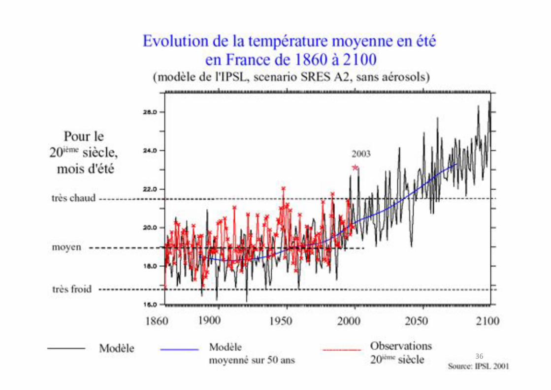
There is substantial evidence, for example, from 13C carbon isotopes in atmospheric CO2 (Keeling et al., 2005) that source/sink processes on land generate most of the interannual variability in the atmospheric CO2 growth rate (Figure 6.12). The strong positive anomalies of the CO2 growth rate in El Niño years (e.g., 1986–1987 and 1997–1998) orig-inated in tropical latitudes (see Sections 6.3.6.3 and 6.3.2.5.4), while the anomalies in 2003 and 2005 originated in northern mid-latitudes, perhaps reflecting the European heat wave in 2003 (Ciais et al., 2005). Volcanic forcing also contributes to multi-annual variability in carbon storage on land and in the ocean (Jones and Cox, 2001; Gerber et al., 2003; Brovkin et al., 2010; Frölicher et al., 2011).

With a very high level of confidence, the increase in CO2 emissions from fossil fuel burning and those arising from land use change are the

dominant cause of the observed increase in atmospheric CO2 concen-tration. Several lines of evidence support this conclusion:

• The observed decrease in atmospheric O2 content over past two decades and the lower O2 content in the northern compared to the SH are consistent with the burning of fossil fuels (see Figure 6.3 and Section 6.1.3.2; Keeling et al., 1996; Manning and Keeling, 2006).

• CO2 from fossil fuels and from the land biosphere has a lower 13C/12C stable isotope ratio than the CO2 in the atmosphere. This induces a decreasing temporal trend in the atmospheric 13C/12C ratio of atmospheric CO2 concentration as well as, on annual aver-age, slightly lower 13C/12C values in the NH (Figure 6.3). These sig-nals are measured in the atmosphere.

• Because fossil fuel CO2 is devoid of radiocarbon (14C), reconstruc-tions of the 14C/C isotopic ratio of atmospheric CO2 from tree rings

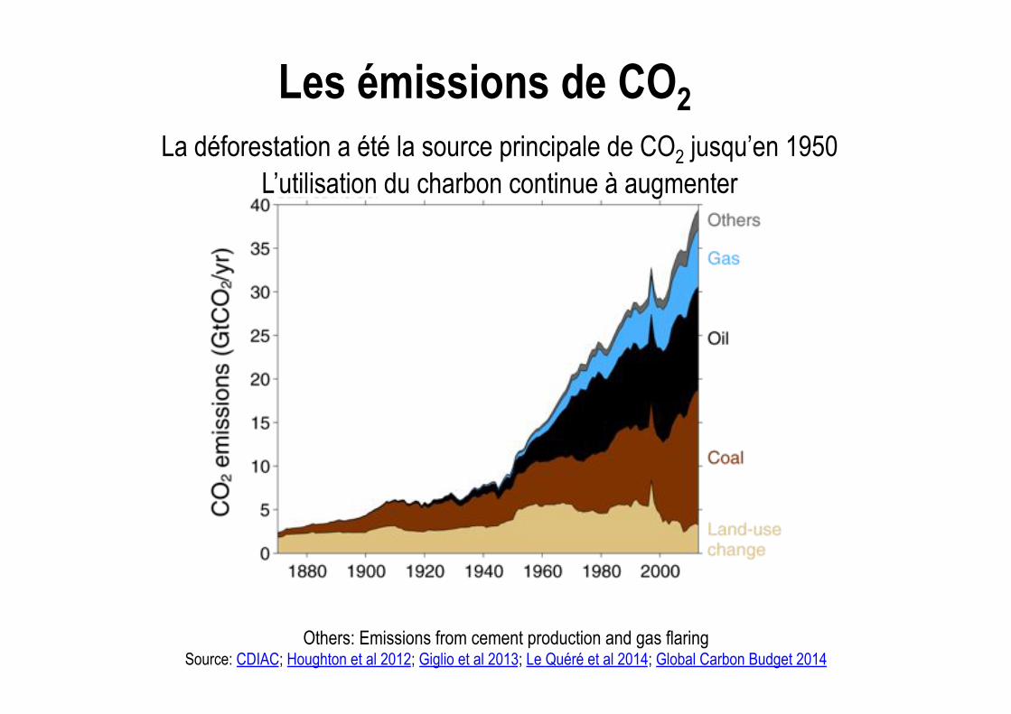
Les émissions de CO2

Others: Emissions from cement production and gas flaring Source: CDIAC; Houghton et al 2012; Giglio et al 2013; Le Quéré et al 2014; Global Carbon Budget 2014

La déforestation a été la source principale de CO2 jusqu’en 1950 L’utilisation du charbon continue à augmenter

9


6

6.1.1.2 Methane Cycle

CH4 absorbs infrared radiation relatively stronger per molecule com-pared to CO2 (Chapter 8), and it interacts with photochemistry. On the other hand, the methane turnover time (see Glossary) is less than 10 years in the troposphere (Prather et al., 2012; see Chapter 7). The sources of CH4 at the surface of the Earth (see Section 6.3.3.2) can be thermogenic including (1) natural emissions of fossil CH4 from geolog-ical sources (marine and terrestrial seepages, geothermal vents and mud volcanoes) and (2) emissions caused by leakages from fossil fuel extraction and use (natural gas, coal and oil industry; Figure 6.2). There are also pyrogenic sources resulting from incomplete burning of fossil fuels and plant biomass (both natural and anthropogenic fires). Last, biogenic sources include natural biogenic emissions predominantly from wetlands, from termites and very small emissions from the ocean (see Section 6.3.3). Anthropogenic biogenic emissions occur from rice

Box 6.1 (continued)

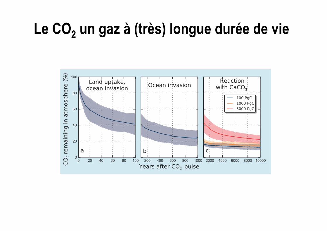
Phase 2. In the second stage, within a few thousands of years, the pH of the ocean that has decreased in Phase 1 will be restored by reaction of ocean dissolved CO2 and calcium carbonate (CaCO3) of sea floor sediments, partly replenishing the buffer capacity of the ocean and further drawing down atmospheric CO2 as a new balance is re-established between CaCO3 sedimentation in the ocean and terrestrial weathering (Box 6.1, Figure 1c right). This second phase will pull the remaining atmospheric CO2 fraction down to 10 to 25% of the original CO2 pulse after about 10 kyr (Lenton and Britton, 2006; Montenegro et al., 2007; Ridgwell and Hargreaves, 2007; Tyrrell et al., 2007; Archer and Brovkin, 2008).

Phase 3. In the third stage, within several hundred thousand years, the rest of the CO2 emitted during the initial pulse will be removed from the atmosphere by silicate weathering, a very slow process of CO2 reaction with calcium silicate (CaSiO3) and other minerals of igneous rocks (e.g., Sundquist, 1990; Walker and Kasting, 1992).

Involvement of extremely long time scale processes into the removal of a pulse of CO2 emissions into the atmosphere complicates comparison with the cycling of the other GHGs. This is why the concept of a single, characteristic atmospheric lifetime is not applicable to CO2 (Chapter 8).

Box 6.1, Figure 1 | A percentage of emitted CO2 remaining in the atmosphere in response to an idealised instantaneous CO2 pulse emitted to the atmosphere in year 0 as calculated by a range of coupled climate–carbon cycle models. (Left and middle panels, a and b) Multi-model mean (blue line) and the uncertainty interval (±2 standard deviations, shading) simulated during 1000 years following the instantaneous pulse of 100 PgC (Joos et al., 2013). (Right panel, c) A mean of models with oceanic and terrestrial carbon components and a maximum range of these models (shading) for instantaneous CO2 pulse in year 0 of 100 PgC (blue), 1000 PgC (orange) and 5000 PgC (red line) on a time interval up to 10 kyr (Archer et al., 2009b). Text at the top of the panels indicates the dominant processes that remove the excess of CO2 emitted in the atmosphere on the successive time scales. Note that higher pulse of CO2 emissions leads to higher remaining CO2 fraction (Section 6.3.2.4) due to reduced carbonate buffer capacity of the ocean and positive climate–carbon cycle feedback (Section 6.3.2.6.6).

paddy agriculture, ruminants, landfills, man-made lakes and wetlands and waste treatment. In general, biogenic CH4 is produced from organ-ic matter under low oxygen conditions by fermentation processes of methanogenic microbes (Conrad, 1996). Atmospheric CH4 is removed primarily by photochemistry, through atmospheric chemistry reactions with the OH radicals. Other smaller removal processes of atmospher-ic CH4 take place in the stratosphere through reaction with chlorine and oxygen radicals, by oxidation in well aerated soils, and possibly by reaction with chlorine in the marine boundary layer (Allan et al., 2007; see Section 6.3.3.3).

A very large geological stock (globally 1500 to 7000 PgC, that is 2 x 106 to 9.3 x 106 Tg(CH4) in Figure 6.2; Archer (2007); with low confi-dence in estimates) of CH4 exists in the form of frozen hydrate deposits (‘clathrates’) in shallow ocean sediments and on the slopes of con-tinental shelves, and permafrost soils. These CH4 hydrates are stable

Le CO2 un gaz à (très) longue durée de vie

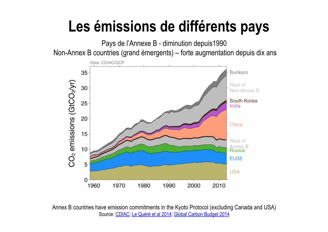
Les émissions de différents pays

Annex B countries have emission commitments in the Kyoto Protocol (excluding Canada and USA) Source: CDIAC; Le Quéré et al 2014; Global Carbon Budget 2014

Pays de l’Annexe B - diminution depuis1990 Non-Annex B countries (grand émergents) – forte augmentation depuis dix ans

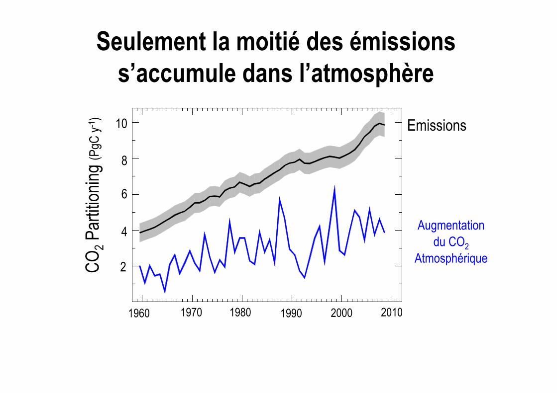
Seulement la moitié des émissions s’accumule dans l’atmosphère

Emissions

Augmentation du CO2

Atmosphérique CO

2 Par

titio

ning

(PgC

y-1

)

1960 2010 1970 1990 2000 1980

10

8

6

4

2

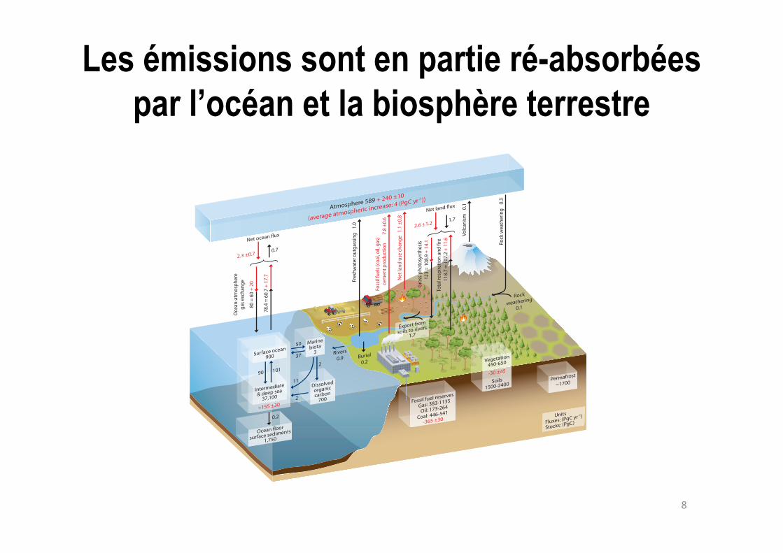
Les émissions sont en partie ré-absorbées par l’océan et la biosphère terrestre

8"

Surface ocean900

Intermediate

& deep sea37,100

+155 ±30

Ocean !oor

surface sediments

1,750

Dissolvedorganiccarbon

700

Marinebiota

3

90 101

50

11

0.2

37

2

2

Rock

weathering

0.1

Fossil fuel reserves

Gas: 383-1135

Oil: 173-264

Coal: 446-541

-365 ±30

Atmosphere 589 + 240 ±10

(average atmospheric increase: 4 (PgC yr -1))

Net ocean !ux

2.3 ±0.70.7

Fres

hwat

er o

utga

ssin

g

Net l

and

use

chan

ge

Foss

il fu

els (

coal

, oil,

gas)

cem

ent p

rodu

ctio

n

1.0

1.1

±0.

8

7.8

±0.6

Gros

s pho

tosy

nthe

sis

123

= 10

8.9

+ 14

.1

Volc

anism

0.1

Rivers0.9 Burial

0.2

Export from

soils to rivers1.7

Units

Fluxes: (PgC yr -1)

Stocks: (PgC)

Rock

wea

ther

ing

0.3

Tota

l res

pira

tion

and

fire

118.

7 =

107.

2 +

11.6

Net land !ux

2.6 ±1.21.7

78.4

= 6

0.7

+ 17

.7

80 =

60

+ 20

Oce

an-a

tmos

pher

ega

s exc

hang

e

Vegetation450-650

-30 ±45

Soils1500-2400

Permafrost

~1700

Bilan global du CO2 anthropique moyenne 2004-2013

Source: CDIAC; NOAA-ESRL; Houghton et al 2012; Giglio et al 2013; Le Quéré et al 2014; Global Carbon Budget 2014

26% 9.4±1.8 GtCO2/yr

32.4±1.6 GtCO2/yr 91%

+ 3.3±1.8 GtCO2/yr 9%

10.6±2.9 GtCO2/yr

29% Calculated as the residual

of all other flux components

15.8±0.4 GtCO2/yr

44%

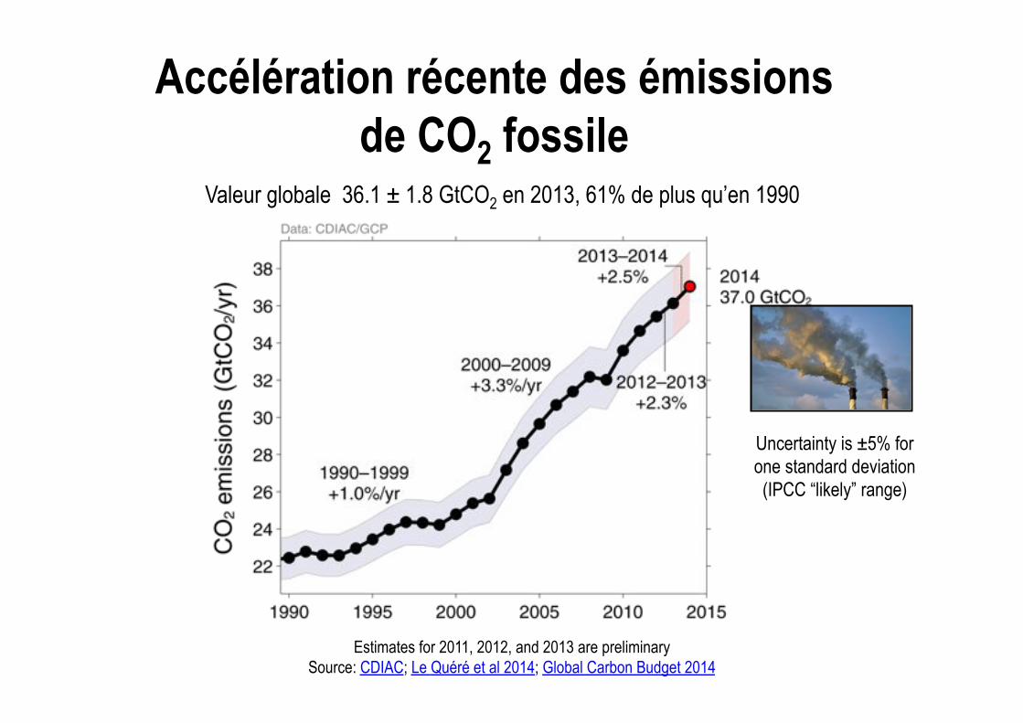
Accélération récente des émissions de CO2 fossile

Valeur globale 36.1 ± 1.8 GtCO2 en 2013, 61% de plus qu’en 1990

Estimates for 2011, 2012, and 2013 are preliminary

Source: CDIAC; Le Quéré et al 2014; Global Carbon Budget 2014

Uncertainty is ±5% for one standard deviation (IPCC “likely” range)

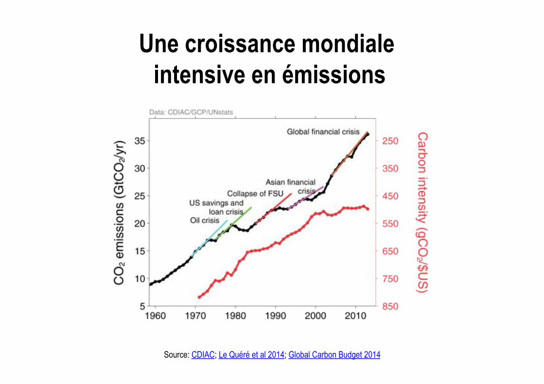
Une croissance mondiale intensive en émissions


Augmentation des émissions de CO2 liées au charbon (2008 to 2010)

CO

2 em

issi

ons

(Tg

C

y-1)

127% of growth

Global Carbon Project 2011; Data: Boden, Marland, Andres-CDIAC 2011

-100

-50

0

50

100

150

200

250

China India Dev. world World Developed World

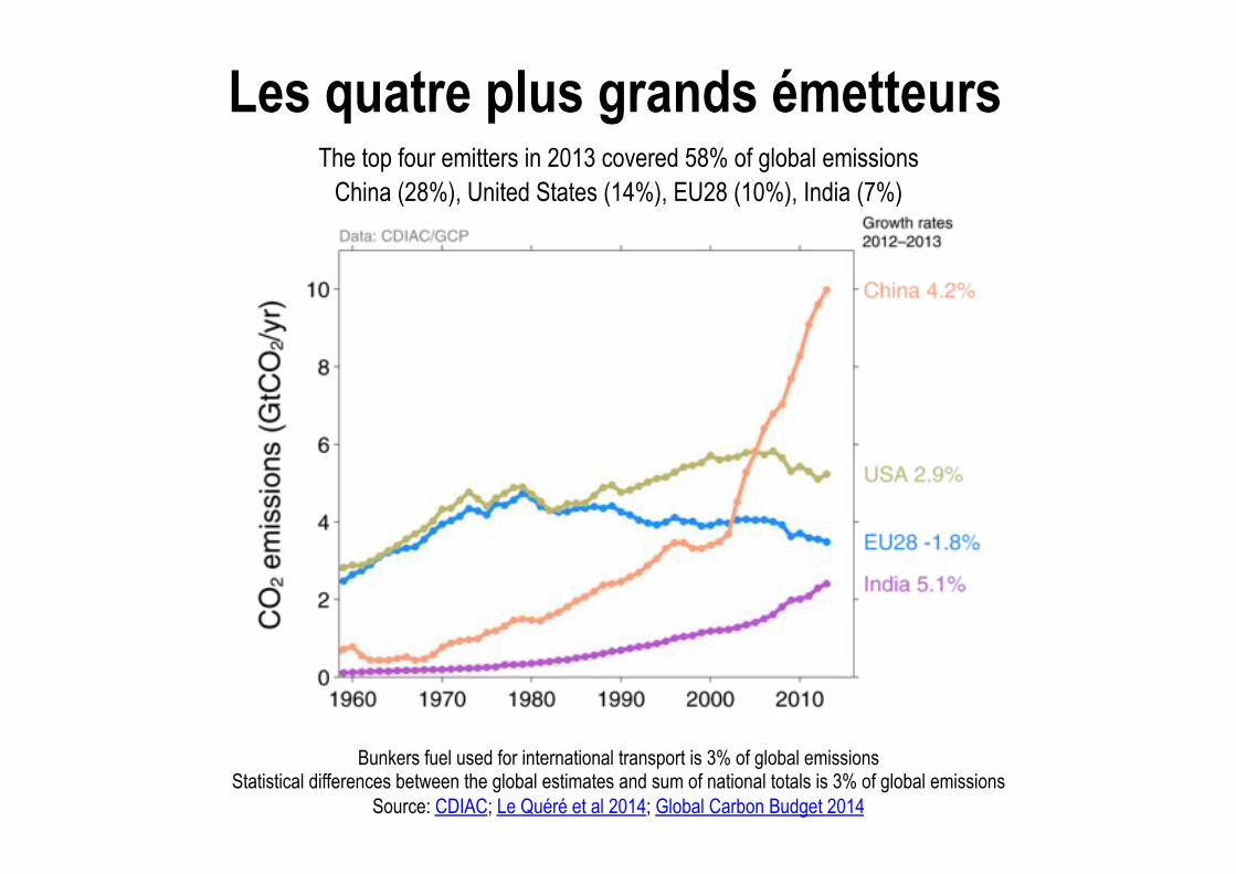
Les quatre plus grands émetteurs The top four emitters in 2013 covered 58% of global emissions

China (28%), United States (14%), EU28 (10%), India (7%)

Bunkers fuel used for international transport is 3% of global emissions Statistical differences between the global estimates and sum of national totals is 3% of global emissions


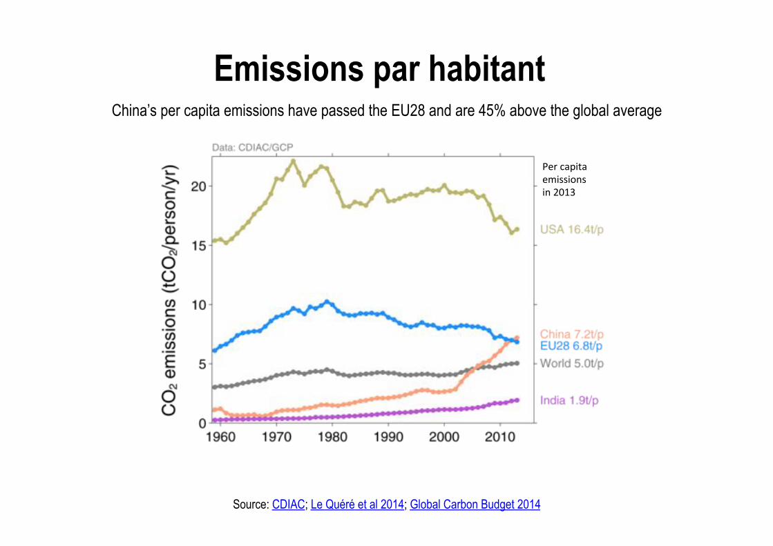
Emissions par habitant China’s per capita emissions have passed the EU28 and are 45% above the global average


Per"capita"emissions"in"2013"

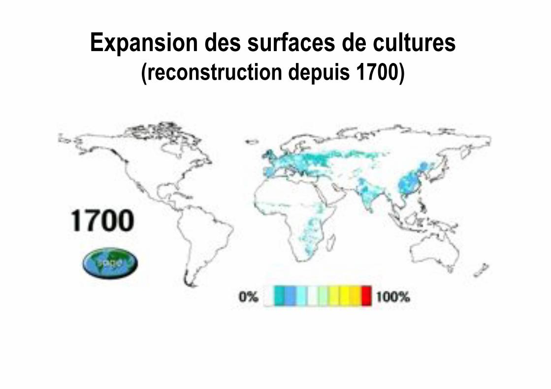
Expansion des surfaces de cultures (reconstruction depuis 1700)

Changements des surfaces forestières (1990-2010)

(FAO 2010)

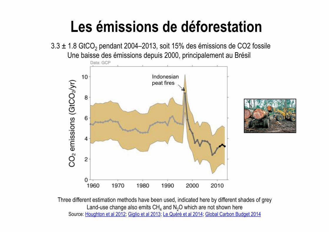
Les émissions de déforestation 3.3 ± 1.8 GtCO2 pendant 2004–2013, soit 15% des émissions de CO2 fossile

Une baisse des émissions depuis 2000, principalement au Brésil

Three different estimation methods have been used, indicated here by different shades of grey Land-use change also emits CH4 and N2O which are not shown here

Source: Houghton et al 2012; Giglio et al 2013; Le Quéré et al 2014; Global Carbon Budget 2014

Indonesian peat fires

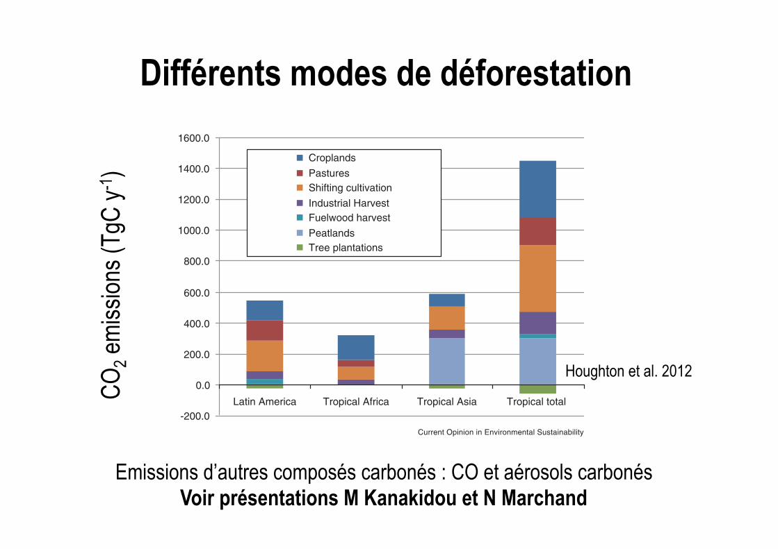
Différents modes de déforestation

(Figure 1). The emissions are large because the changesin carbon density are large when forests are converted tocroplands. Essentially all the initial vegetation is replacedby crops, so if the carbon density of the initial biomass isknown, it is, in principle, straightforward to calculate thenet loss of carbon associated with clearing. Additionalsources of uncertainty include estimating the time it takesfor the release or uptake of carbon to occur. How much ofthe biomass is burned at the time of clearing? How muchwoody material is removed from site (wood products) andnot decayed immediately? Answers vary across regionsand through time (e.g. [23]). Estimates of annual sourcesand sinks depend on the answers, yet site-specific data aregenerally lacking. A few case studies usually provide thevalues used in calculation of carbon emissions and uptakeover large regions.

On average, soil carbon in the upper meter of soil isreduced by 25–30% as a result of cultivation, and thisaverage has been documented in a large number ofreviews [24–27]. There is some variation about this aver-age, but the loss is broadly robust across all ecosystems,despite the variety of soil types, cultivation practices, anddecomposition processes.

Draining and burning of peatlandsThe draining and burning of peatlands for the productionof oil palm in Southeast Asia are estimated to causeaverage annual emissions of 0.3 PgC yr!1 [3]. This

activity has not been explicitly included in the modelinganalysis reported here, but the emissions have beenadded to Figure 1 and Table 1 because the activity isassociated with deforestation. At 0.3 PgC yr!1, the drain-ing and burning of peatlands is the activity with the thirdhighest emissions (Figure 1).

PasturesThe expansion of pastures in the tropics over the lastdecades is estimated to have released 0.180 PgC yr!1

(Figure 1), the fourth largest net flux from land-usechange. Cattle pastures in Latin America are a majordriver of deforestation in that region.

The net emissions of carbon from changes in pasture areaare less than the emissions from cropland expansion, first,because more forests are converted to shifting cultivationand croplands than to pastures, and, second, becausepastures are generally not cultivated, and thus lose littlecarbon from soils. The changes in soil organic carbon(SOC) resulting from the conversion of forests to pasturesare highly variable, however, with both increases anddecreases observed.

Harvest of industrial woodThe harvest of industrial wood (e.g. timber, pulp) wasresponsible for a net loss of 0.141 PgC yr!1 over the lasttwo decades (Table 1). This net flux from wood harvestincludes both the emissions from the burning and decay

4 Climate systems

COSUST-221; NO. OF PAGES 7

Please cite this article in press as: Houghton RA. Carbon emissions and the drivers of deforestation and forest degradation in the tropics, Curr Opin Environ Sustain (2012), http://dx.doi.org/10.1016/j.cosust.2012.06.006

Figure 1

-200.0

0.0

200.0

400.0

600.0

800.0

1000.0

1200.0

1400.0

1600.0

Latin America Tropical Africa Tropical Asia Tropical total

CroplandsPasturesShifting cultivationIndustrial HarvestFuelwood harvestPeatlandsTree plantations

Current Opinion in Environmental Sustainability

Sources (+) and sinks (!) of carbon (TgC yr!1) from activities contributing to deforestation and forest degradation in tropical regions.

Current Opinion in Environmental Sustainability 2012, 4:1–7 www.sciencedirect.com

Houghton et al. 2012

CO

2 em

issi

ons

(TgC

y-1

)

Emissions d’autres composés carbonés : CO et aérosols carbonés Voir présentations M Kanakidou et N Marchand

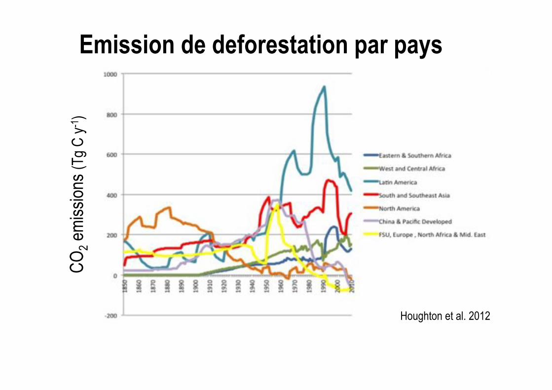
Emission de deforestation par pays

Houghton et al. 2012

CO

2 em

issi

ons

(Tg

C y

-1)

C. Le Quéré et al.: Global carbon budget 2013 255

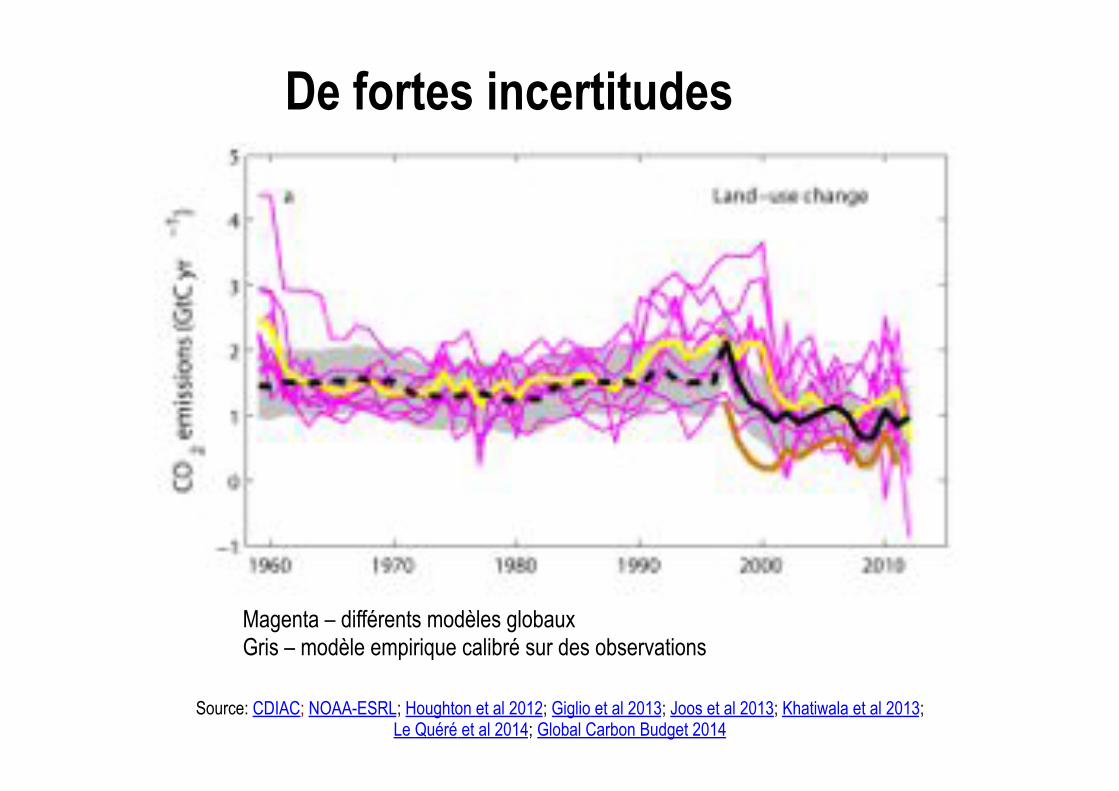
Figure 5. Comparison between the CO2 budget values estimatedhere (black line), and other methods and models (Table 6; colouredlines) for (a) CO2 emissions from land-use change showing indi-vidual DGVM model results (magenta) and the multi model mean(yellow line), and fire-based results (orange), LUC data prior to1997 (dashed black line) highlights the start of satellite data fromthat year (b) land CO2 sink (SLAND) showing individual DGVMmodel results (green) and multi model mean (yellow line), and (c)ocean CO2 sink (SOCEAN) showing individual models before nor-malisation (blue lines), and the two data-based products (red line forRödenbeck et al. (2014) and purple line for Park et al., 2010). Bothdata-based products were corrected for the preindustrial source ofCO2 from riverine input to the ocean, which is not present in themodels, by adding a sink of 0.45GtC yr�1 (Jacobson et al., 2007),to make them comparable to SOCEAN .

Figure 6. Comparison of global carbon budget components re-leased annually by GCP since 2005. CO2 emissions from both (a)fossil-fuel combustion and cement production (EFF), and (b) land-use change (ELUC), and their partitioning among (c) the atmo-sphere (GATM), (d) the ocean (SOCEAN), and (e) the land (SLAND).See legend for the corresponding years, with the 2006 carbon bud-get from Raupach et al. (2007); 2007 from Canadell et al. (2007); to2008 published online only; 2009 from Le Quéré et al. (2009); 2010from Friedlingstein et al. (2010); 2011 from Peters et al. (2012b);2012 from Le Quéré et al. (2013); and this year’s budget (2013).The budget year generally corresponds to the year when the budgetwas first released. All values are in GtC yr�1.

The DGVMs thus estimate internally consistent land fluxesover 2012, with both ELUC and SLAND being weaker thanthose of the carbon budget. Internal consistency is an emerg-ing property of the models, not an a priori constraint as is theresidual calculation of SLAND. These results thus suggest thatconstraints from DGVMs may provide sufficient informationto be directly incorporated in the budget calculations in thefuture.

3.3 Cumulative emissions

Cumulative emissions for 1870–2012 were 380± 20GtC forEFF, and 145± 55GtC for ELUC based on the bookkeepingmethod of Houghton et al. (2012) for 1870–2010, with anextension to 2012 based on methods described in Sect. 2.2(Table 10). The cumulative emissions are rounded to thenearest 5GtC. The total cumulative emissions for 1870–2012 are 525± 55GtC. These emissions were partitionedamong the atmosphere (220± 5GtC) based on atmospheric

www.earth-syst-sci-data.net/6/235/2014/ Earth Syst. Sci. Data, 6, 235–263, 2014

De fortes incertitudes

Source: CDIAC; NOAA-ESRL; Houghton et al 2012; Giglio et al 2013; Joos et al 2013; Khatiwala et al 2013; Le Quéré et al 2014; Global Carbon Budget 2014

Magenta – différents modèles globaux Gris – modèle empirique calibré sur des observations

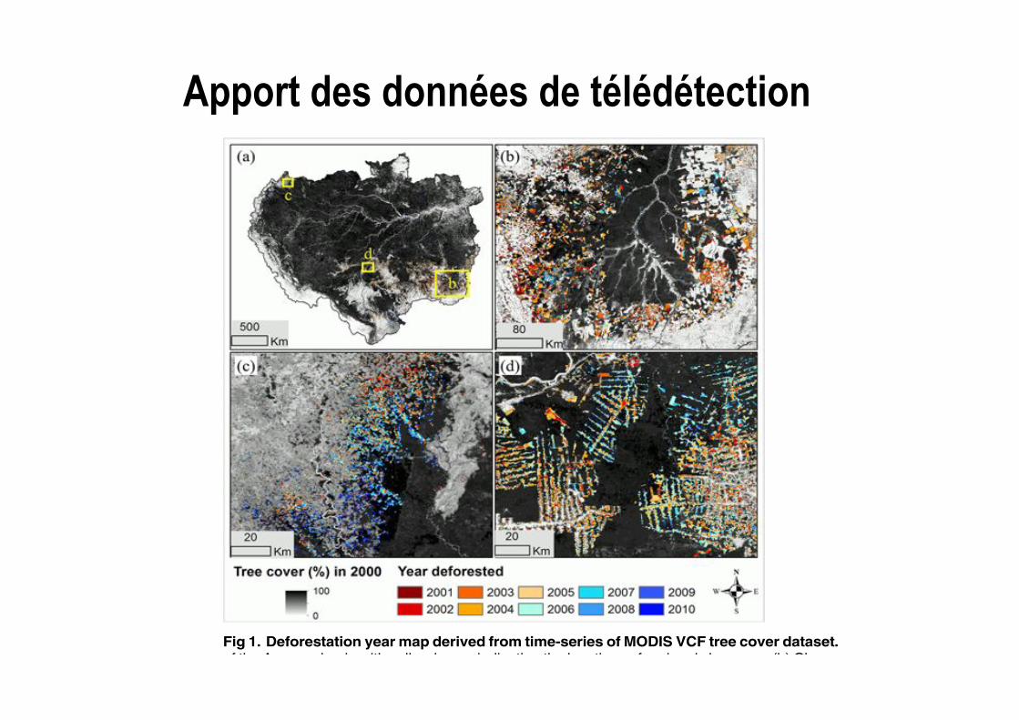
Apport des données de télédétection

Following Brazil, Bolivia contributed the second most deforestation in the last decade, whichaccounted for 12% (1,969 ± 212 K ha) of the basin total, more than the sum of the PeruvianAmazon (6%, or 979 ± 123 K ha) and the Colombian Amazon (2%, or 287 ± 67 K ha).

The geographic locations of deforestation were largely concentrated on the southeasternedge of the basin (the so called “arc of deforestation”), with new hotspots emerging in westernAmazon (Fig 2). Consistent with reports by the Brazilian government, the FAO and other pre-vious studies [14, 46–48], a declining trend in the Brazilian Amazon and the entire Amazonbasin after 2005 was confirmed (Fig 3). The annual relative share of Brazil’s deforestationchanged dramatically over the study period−from the highest of 87% in the year 2004 to thelowest of 54% by the year 2010. The largest decline in deforestation rate was observed in MatoGrosso, from 1,200 K ha in 2004 to below 100 K ha in 2010. Obvious declines were also ob-served in Rondonia and Para, though to lesser degrees. These three states accounted for morethan 80% of forest clearing in Brazil. In the western and southern parts of the basin, deforesta-tion rates in the Peruvian Amazon and the Bolivian Amazon also decreased slightly after 2006.In the Colombian Amazon, annual rates nearly doubled from 2006 to 2009, although the totalarea cleared there was much lower than those in the other countries or states.

Deforestation estimates derived through this study were comparable to those derived basedon Landsat data. At individual patch level, the deforestation maps derived through this studyhad spatiotemporal patterns similar to the PRODES (Program for the Annual Estimation ofDeforestation in the Brazilian Amazon) product [48] and a Landsat-based global forest coverloss (GFCL) dataset [14] (Fig 4). At the state-level, annual deforestation rates derived throughthis study were highly correlated with those calculated based on the two Landsat-based

Fig 1. Deforestation year map derived from time-series of MODIS VCF tree cover dataset. (a) Overviewof the Amazon basin with yellow boxes indicating the locations of regional close-ups. (b) Close-up over theXingu river basin in Mato Grosso, Brazil. The large patch of remaining intact forest is a consequence ofprotection status in this area. (c) Close-up in Colombia. (d) Close-up in Rondonia, Brazil.

doi:10.1371/journal.pone.0126754.g001

Carbon Emissions from Deforestation

PLOS ONE | DOI:10.1371/journal.pone.0126754 May 7, 2015 4 / 21

Source: CDIAC; NOAA-ESRL; Houghton et al 2012; Giglio et al 2013; Le Quéré et al 2014; Global Carbon Budget 2014

26% 9.4±1.8 GtCO2/yr

32.4±1.6 GtCO2/yr 91%

+ 3.3±1.8 GtCO2/yr 9%

10.6±2.9 GtCO2/yr

29% Calculated as the residual

of all other flux components

15.8±0.4 GtCO2/yr

44%

Séparer l’absorption du CO2 entre océan et continents

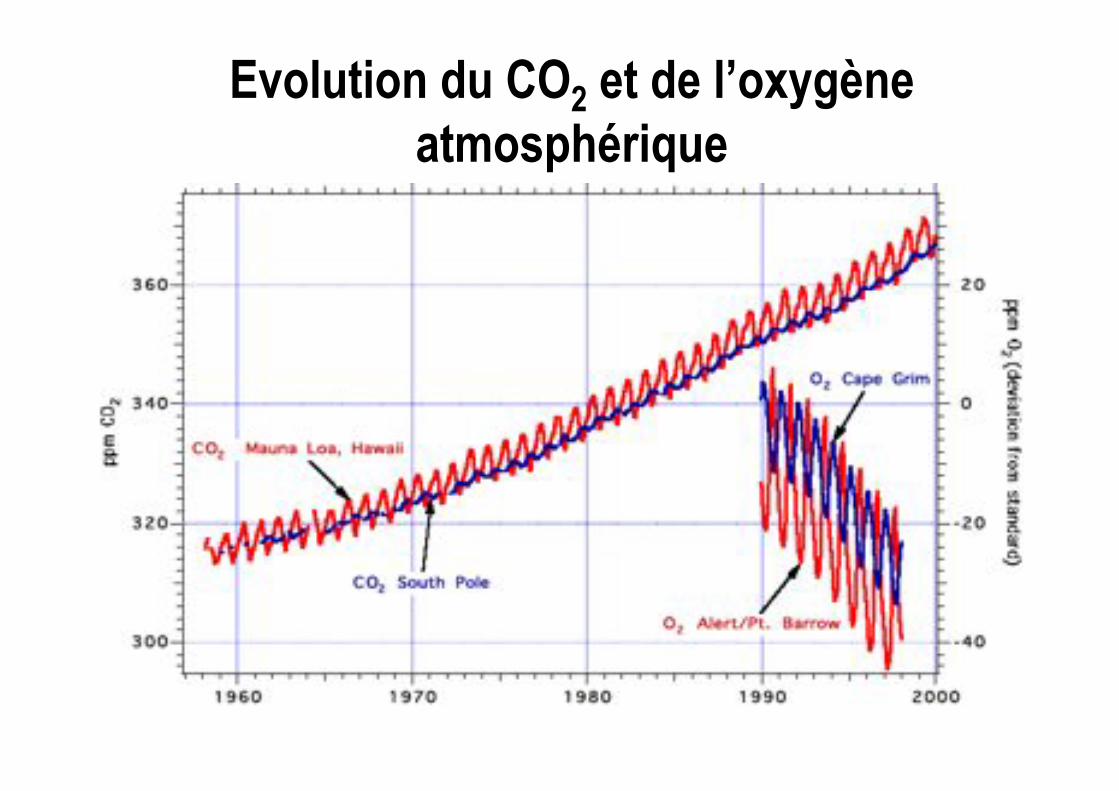
Evolution du CO2 et de l’oxygène atmosphérique

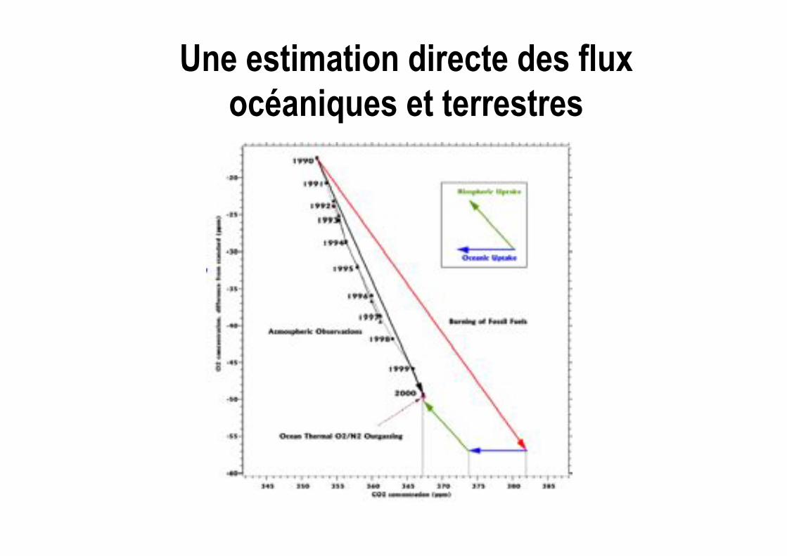
Une estimation directe des flux océaniques et terrestres

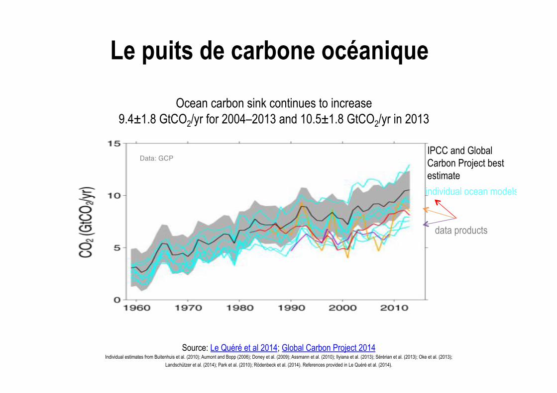
Le puits de carbone océanique

Ocean carbon sink continues to increase 9.4±1.8 GtCO2/yr for 2004–2013 and 10.5±1.8 GtCO2/yr in 2013

Source: Le Quéré et al 2014; Global Carbon Project 2014 Individual estimates from Buitenhuis et al. (2010); Aumont and Bopp (2006); Doney et al. (2009); Assmann et al. (2010); Ilyiana et al. (2013); Sérérian et al. (2013); Oke et al. (2013);

Landschützer et al. (2014); Park et al. (2010); Rödenbeck et al. (2014). References provided in Le Quéré et al. (2014).

Data: GCPIPCC and Global Carbon Project best estimate

individual ocean models

data products

Variations interannuelles de l’accumulation du CO2

The atmospheric concentration growth rate has shown a steady increase The growth in 2013 reflects the growth in fossil emissions, with small changes in the sinks

Source: NOAA-ESRL; Global Carbon Budget 2014

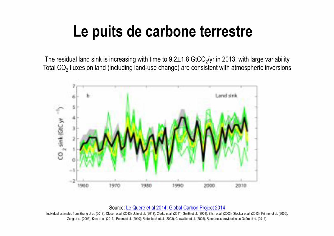
The residual land sink is increasing with time to 9.2±1.8 GtCO2/yr in 2013, with large variability Total CO2 fluxes on land (including land-use change) are consistent with atmospheric inversions

Source: Le Quéré et al 2014; Global Carbon Project 2014 Individual estimates from Zhang et al. (2013); Oleson et al. (2013); Jain et al. (2013); Clarke et al. (2011); Smith et al. (2001); Sitch et al. (2003); Stocker et al. (2013); Krinner et al. (2005);

Zeng et al. (2005); Kato et al. (2013); Peters et al. (2010); Rodenbeck et al. (2003); Chevallier et al. (2005). References provided in Le Quéré et al. (2014).








Le puits de carbone terrestre

En résumé

23


6

in terrestrial ecosystems: the carbon ‘sinks’ (Figure 6.8). The ocean stored 155 ± 30 PgC of anthropogenic carbon since 1750 (see Sec-tion 6.3.2.5.3 and Box 6.1). Terrestrial ecosystems that have not been affected by land use change since 1750, have accumulated 160 ± 90 PgC of anthropogenic carbon since 1750 (Table 6.1), thus not fully compensating the net CO2 losses from terrestrial ecosystems to the atmosphere from land use change during the same period estimated of 180 ± 80 PgC (Table 6.1). The net balance of all terrestrial ecosys-

Figure 6.8 | Annual anthropogenic CO2 emissions and their partitioning among the atmosphere, land and ocean (PgC yr–1) from 1750 to 2011. (Top) Fossil fuel and cement CO2 emissions by category, estimated by the Carbon Dioxide Information Analysis Center (CDIAC) based on UN energy statistics for fossil fuel combustion and US Geological Survey for cement production (Boden et al., 2011). (Bottom) Fossil fuel and cement CO2 emissions as above. CO2 emissions from net land use change, mainly deforestation, are based on land cover change data and estimated for 1750–1850 from the average of four models (Pongratz et al., 2009; Shevliakova et al., 2009; van Minnen et al., 2009; Zaehle et al., 2011) before 1850 and from Houghton et al. (2012) after 1850 (see Table 6.2). The atmospheric CO2 growth rate (term in light blue ‘atmosphere from measurements’ in the figure) prior to 1959 is based on a spline fit to ice core observations (Neftel et al., 1982; Friedli et al., 1986; Etheridge et al., 1996) and a synthesis of atmospheric measurements from 1959 (Ballantyne et al., 2012). The fit to ice core observations does not capture the large interannual variability in atmospheric CO2 and is represented with a dashed line. The ocean CO2 sink prior to 1960 (term in dark blue ‘ocean from indirect observations and models’ in the figure) is from Khatiwala et al. (2009) and from a combination of models and observations from 1960 from (Le Quéré et al., 2013). The residual land sink (term in green in the figure) is computed from the residual of the other terms, and represents the sink of anthropogenic CO2 in natural land ecosystems. The emissions and their partitioning only include the fluxes that have changed since 1750, and not the natural CO2 fluxes (e.g., atmospheric CO2 uptake from weathering, outgassing of CO2 from lakes and rivers, and outgassing of CO2 by the ocean from carbon delivered by rivers; see Figure 6.1) between the atmosphere, land and ocean reservoirs that existed before that time and still exist today. The uncertainties in the various terms are discussed in the text and reported in Table 6.1 for decadal mean values.

cementgasoilcoal

fossil fuel and cement from energy statisticsland use change from data and modelsresidual land sinkmeasured atmospheric growth rateocean sink from data models

1750 1800 1850 1900 1950 2000

10

5

5

10

0

5

10

0

1750 1800 1850 1900 1950 2000

emissions

partitioning

Annu

al anth

ropog

enic C

O 2 emiss

ions

and p

artitio

ning (

PgC y

r –1)

Fossi

l fuel a

nd ce

ment

CO2 em

ission

s (Pg

C yr –1

)

Year

tems, those affected by land use change and the others, is thus close to neutral since 1750, with an average loss of 30 ± 45 (see Figure 6.1). This increased storage in terrestrial ecosystems not affected by land use change is likely to be caused by enhanced photosynthesis at higher CO2 levels and nitrogen deposition, and changes in climate favouring carbon sinks such as longer growing seasons in mid-to-high latitudes. Forest area expansion and increased biomass density of forests that result from changes in land use change are also carbon sinks, and they

Depuis 1750, les émissions cumulées sont de 2000 ± 300 GtCO2 soit 2/3 des émissions totales compatibles avec un réchauffement de 2°C

Les émissions de CO2 fossile étaient de 36.1 ± 1.8 GtCO2 en 2013, 61% plus qu’en 1990

Depuis 50 ans, environ 44% des émissions sont restées dans l’atmosphère, acroissant l’effet de serre de notre planète

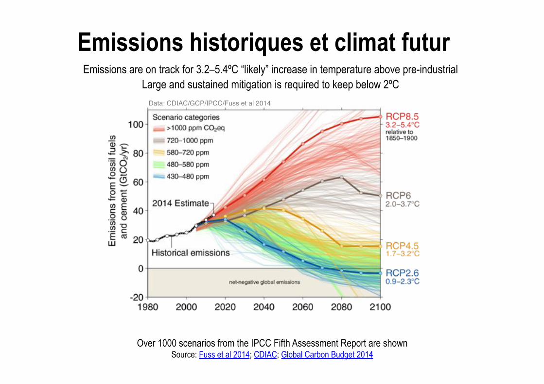
Emissions historiques et climat futur Emissions are on track for 3.2–5.4ºC “likely” increase in temperature above pre-industrial

Large and sustained mitigation is required to keep below 2ºC

Over 1000 scenarios from the IPCC Fifth Assessment Report are shown Source: Fuss et al 2014; CDIAC; Global Carbon Budget 2014

Data: CDIAC/GCP/IPCC/Fuss et al 2014

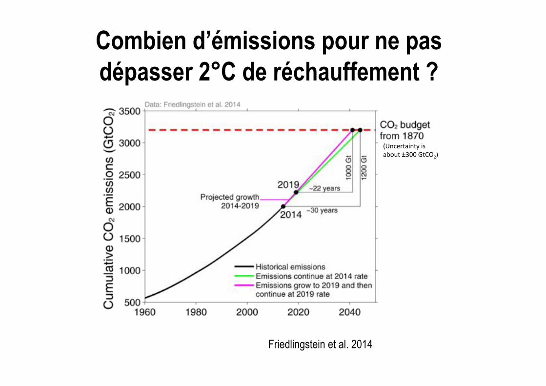
Combien d’émissions pour ne pas dépasser 2°C de réchauffement ?

Cumulative CO2 emissions should remain below about 3200 Gt for a 66% chance of staying below 2°C At present emissions rates the remaining budget would be used up in about 30 years

If emissions continue to grow as projected to 2019 and then continue at the 2019 rate, the remaining budget would be used up about 22 years from 2019

Source: Friedlingstein et al 2014

(Uncertainty"is"about"±300"GtCO2)"

Friedlingstein et al. 2014

Trois grandes questions de recherche

sur l’évolution du cycle du carbone depuis 150 ans

31


6

!

!!

!

!

!

!!!

!

!!!

!

!

!!!

!! !!!!

!

!

!

!!

!!!!

!

!

!!!!

!

!

!

!

!

!!

!

!!!

!

! !

2 3 4 5 6 7 8 9

0

1

2

3

4

Qfoss,N!Qfoss,S !PgC yr!1"

C MLO!C

SPO!ppm"

Figure 6.13 | Blue points: Annually averaged CO2 concentration difference between the station Mauna Loa in the Northern Hemisphere and the station South Pole in the Southern Hemisphere (vertical axis; Keeling et al., 2005, updated) versus the differ-ence in fossil fuel combustion CO2 emissions between the hemispheres (Boden et al., 2011). Dark red dashed line: regression line fitted to the data points.

6.3.2.4 Carbon Dioxide Airborne Fraction

Until recently, the uncertainty in CO2 emissions from land use change emissions was large and poorly quantified which led to the use of an airborne fraction (see Glossary) based on CO2 emissions from fossil fuel only (e.g., Figure 7.4 in AR4 and Figure 6.26 of this chapter). However, reduced uncertainty of emissions from land use change and larger agreement in its trends over time (Section 6.3.2.2) allow making use of an airborne fraction that includes all anthropogenic emissions. The airborne fraction will increase if emissions are too fast for the uptake of CO2 by the carbon sinks (Bacastow and Keeling, 1979; Gloor et al., 2010; Raupach, 2013). It is thus controlled by changes in emissions rates, and by changes in carbon sinks driven by rising CO2, changes in climate and all other biogeochemical changes.

A positive trend in airborne fraction of ~0.3% yr–1 relative to the mean of 0.44 ±0.06 (or about 0.05 increase over 50 years) was found by all recent studies (Raupach et al., 2008, and related papers; Knorr, 2009; Gloor et al., 2010) using the airborne fraction of total anthropogenic CO2 emissions over the approximately 1960–2010 period (for which the most accurate atmospheric CO2 data are available). However, there is no consensus on the significance of the trend because of differences in the treatment of uncertainty and noise (Raupach et al., 2008; Knorr, 2009). There is also no consensus on the cause of the trend (Canadell et al., 2007b; Raupach et al., 2008; Gloor et al., 2010). Land and ocean carbon cycle model results attributing the trends of fluxes to underly-ing processes suggest that the effect of climate change and variability on ocean and land sinks have had a significant influence (Le Quéré et al., 2009), including the decadal influence of volcanic eruptions (Fröli-cher et al., 2013).

6.3.2.5 Ocean Carbon Dioxide Sink

6.3.2.5.1 Global ocean sink and decadal change

The estimated mean anthropogenic ocean CO2 sink assessed in AR4 was 2.2 ± 0.7 PgC yr–1 for the 1990s based on observations (McNeil et al., 2003; Manning and Keeling, 2006; Mikaloff-Fletcher et al., 2006), and is supported by several contemporary estimates (see Chapter 3). Note that the uncertainty of ±0.7 PgC yr–1 reported here (90% confi-dence interval) is the same as the ±0.4 PgC yr–1 uncertainty reported in AR4 (68% confidence intervals). The uptake of anthropogenic CO2 by the ocean is primarily a response to increasing CO2 in the atmos-

Park et al. (2010)

b. CO effect only2

a. Climate effect only

Assmann et al. (2010)

Graven et al. (2012)

updated from Le Quere et al. (2010)

updated from Doney et al. (2009)

updated from Khatiwala et al.(2009)

c. CO and climate effects combined2

Year

1960 1970 1980 1990 2000 2010

1960 1970 1980 1990 2000 2010

1960 1970 1980 1990 2000 2010

1

0

-1

1

0

-1

1

0

-1

Oce

an C

Osi

nk a

nom

alie

s (P

gC y

r)

2

-1

Figure 6.14 | Anomalies in the ocean CO2 ocean-to-atmosphere flux in response to (a) changes in climate, (b) increasing atmospheric CO2 and (c) the combined effects of increasing CO2 and changes in climate (PgC yr–1). All estimates are shown as anomalies with respect to the 1990–2000 averages. Estimates are updates from ocean models (in colours) and from indirect methods based on observations (Khati-wala et al., 2009; Park et al., 2010). A negative ocean-to-atmosphere flux represents a sink of CO2, as in Table 6.1.

Evolution du gradient inter-hémisphérique de CO2

La différence de puits naturels entre les deux hémisphères a évolué

proportionnellement aux émissions depuis 50 ans

CO2 P

artit

ioni

ng (P

gC y

-1)

1960 2010 1970 1990 2000 1980

10

8

6

4

2

La fraction des émissions absorbée par les réservoirs naturelle est très stable, malgré la très forte augmentation du

forçage des émissions

Quasi-linéarité de la réponse globale du cycle du carbone

Ce)e$linéarité$va$t’elle$con5nuer$dans$le$futur$?$$Voir$présenta5on$de$L.$Bopp$

Le plateau de CO2 des années 1940

Tem

péra

ture

60-

90°N

La variabilité décennale des flux de CO2

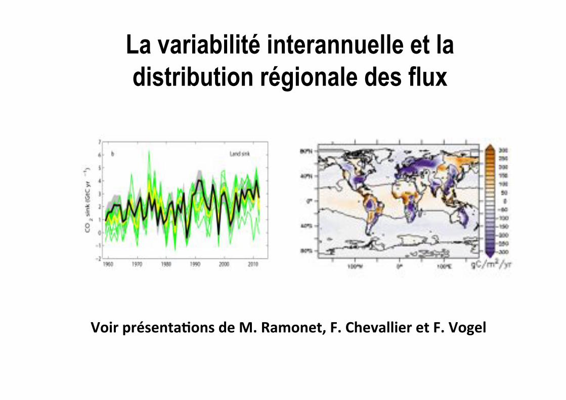
La variabilité interannuelle et la distribution régionale des flux








Voir$présenta5ons$de$M.$Ramonet,$F.$Chevallier$et$F.$Vogel$

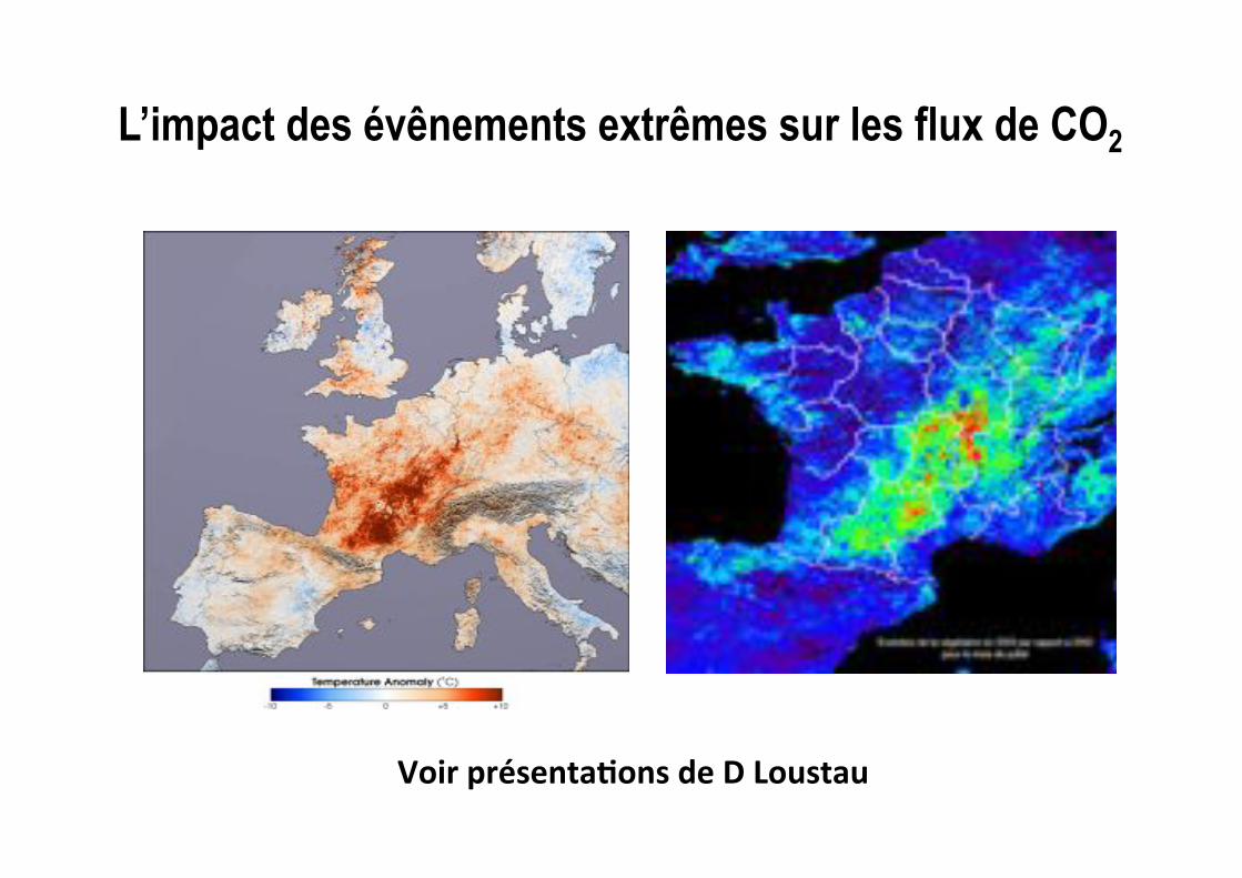
L’impact des évênements extrêmes sur les flux de CO2

Voir$présenta5ons$de$D$Loustau$$

More information, data sources and data files: www.globalcarbonproject.org

Contact: [email protected]

More information, data sources and data files: www.globalcarbonatlas.org

Contact: [email protected]

Données sur le bilan global annuel de CO2 anthropique

Corinne Le Quéré Tyndall Centre for Climate Change Research, Uni. of East Anglia, UK Róisín Moriarty Tyndall Centre for Climate Change Research, Uni. of East Anglia, UK Robbie Andrew Center for International Climate & Environmental Research - Oslo (CICERO), Norway Glen Peters Center for International Climate & Environmental Research - Oslo (CICERO), Norway Pierre Friedlingstein College of Engineering, Mathematics & Physical Sciences, Uni. of Exeter, UK Mike Raupach Climate Change Institute, Australian National University, Australia Pep Canadell Global Carbon Project, CSIRO Marine & Atmospheric Research, Australia Philippe Ciais LSCE, CEA-CNRS-UVSQ, France Steve Jones Tyndall Centre for Climate Change Research, Uni. of East Anglia, UK Stephen Sitch College of Life & Environmental Sciences Uni. of Exeter, UK Pieter Tans Nat. Oceanic & Atmospheric Admin., Earth System Research Laboratory (NOAA/ESRL), US Almut Arneth Karlsruhe Inst. of Tech., Inst. Met. & Climate Res./Atmospheric Envir. Res., Germany Tom Boden Carbon Dioxide Information Analysis Center (CDIAC), Oak Ridge National Laboratory, US Laurent Bopp LSCE, CEA-CNRS-UVSQ, France Yann Bozec CNRS, Station Biologique de Roscoff, Roscoff, France Frédéric Chevallier LSCE, CEA-CNRS-UVSQ, France Cathy Cosca Nat. Oceanic & Atmospheric Admin. & Pacific Mar. Env. Lab. (NOAA/PMEL), US Harry Harris Climatic Research Unit (CRU), Uni. of East Anglia, UK Mario Hoppema AWI Helmholtz Centre for Polar and Marine, Bremerhaven, Germany Skee Houghton Woods Hole Research Centre (WHRC), US Jo House Cabot Inst., Dept. of Geography, University of Bristol, UK Atul Jain Dept. of Atmospheric Sciences, Uni. of Illinois, US Truls Johannessen Geophysical Inst., Uni. of Bergen & Bjerknes Centre for Climate Research, Norway Etsushi Kato Center for Global Envir. Research (CGER), Nat. Inst. for Envir. Studies (NIES), Japan Ralph Keeling Uni. of California - San Diego, Scripps Institution of Oceanography, US Kees Klein Goldewijk PBL Netherlands Envir. Assessment Agency & Utrecht Uni., Netherlands Vassillis Kitidi Plymouth Marine Laboratory, Plymouth, UK Charles Koven Earth Sciences Division, Lawrence Berkeley National Lab, US Camilla Landa Geophysical Inst., Uni. of Bergen & Bjerknes Centre for Climate Research, Norway Peter Landschützer Environmental Physics Group, IBPD, ETH Zürich, Switzerland Andy Lenton CSIRO Marine and Atmospheric Research, Hobart, Tasmania, Australia Ivan Lima Woods Hole Oceanographic Institution (WHOI), Woods Hole, US Gregg Marland Research Inst. for Environment, Energy & Economics, Appalachian State Uni., US Jeremy Mathis Nat. Oceanic & Atmospheric Admin. & Pacific Mar. Env. Lab. (NOAA/PMEL), US Nicholas Metzl Sorbonne Universités, CNRS, IRD, MNHN, LOCEAN/IPSL Laboratory, Paris, France Yukihiro Nojiri Center for Global Envir. Research (CGER), Nat. Inst. for Envir. Studies (NIES), Japan Are Olsen Geophysical Inst., Uni. of Bergen & Bjerknes Centre for Climate Research, Norway Tsuneo Ono Fisheries Research Agency, Japan Wouter Peters Department of Meteorology and Air Quality, Wageningen Uni., Netherlands Benjamin Pfeil Geophysical Inst., Uni. of Bergen & Bjerknes Centre for Climate Research, Norway Ben Poulter LSCE, CEA-CNRS-UVSQ, France

Pierre Regnier Dept. of Earth & Environmental Sciences, Uni. Libre de Bruxelles, Belgium Christian Rödenbeck Max Planck Institute for Biogeochemistry, Germany Shu Saito Marine Division, Global Environment & Marine Dept., Japan Meteorological Agency, Japan Joe Sailsbury Ocean Processes Analysis Laboratory, Uni. of New Hampshire, US Ute Schuster College of Engineering, Mathematics & Physical Sciences, Uni. of Exeter, UK Jörg Schwinger Geophysical Inst., Uni. of Bergen & Bjerknes Centre for Climate Research, Norway Roland Séférian CNRM-GAME, Météo-France/CNRS, Toulouse, France Joachim Segschneider Max Planck Institute for Meteorology, Germany Tobias Steinhoff GEOMAR Helmholtz Centre for Ocean Research, Kiel, Germany Beni Stocker Physics Inst., & Oeschger Centre for Climate Change Research, Uni. of Bern, Switzerland Adrianna Sutton Joint Inst. for the Study of the Atm. & Ocean, Uni. of Washington & NOAA/PMEL, US Taka Takahashi Lamont-Doherty Earth Observatory of Columbia University, Palisades, US Brönte Tilbrook CSIRO Marine & Atm. Res., Antarctic Cli. & Ecosystems Co-op. Res. Centre, Australia Guido van der Werf Faculty of Earth and Life Sciences, VU University Amsterdam, The Netherlands Nicolas Viovy LSCE, CEA-CNRS-UVSQ, France Ying-Ping Wang CSIRO Ocean and Atmosphere, Victoria, Australia Rik Wanninkhof NOAA/AOML, US Andy Wiltshire Met Office Hadley Centre, UK Ning Zeng Department of Atmospheric and Oceanic Science, Uni. of Maryland, US

Freidlingstein et al. 2014, Raupach et al. 2014 & Fuss et al. 2014 (not already mentioned above) J Rogelj Inst. for Atm. and Climate Science ETH Zürich, Switzerland & IIASA, Laxemburg, Austria R Knutti Inst. for Atm. and Climate Science ETH Zürich, Switzerland G Luderer Potsdam Institute for Climate Impact Research (PIK), Potsdam, Germany M Schaefer Climate Analytics, Berlin, Germany & Env. Sys. Anal. Agency, Wageningen Uni., Netherlands Detlef van Vuuren PBL Netherlands Env. Assess. Agency, Bilthoven & CISD,Utrecht Uni., Netherlands Steven David Department of Earth System Science, University of California, California, US Frank Jotzo Crawford School of Public Policy, Australian National University, Canberra, Australia Sabine Fuss Mercator Research Institute on Global Commons & Climate Change, Berlin, Germany Massimo Tavoni FEEM, CMCC & Politecnico di Milano, Milan, Italy Rob Jackson School of Earth Sci., Woods Inst. for the Env., & Percourt Inst. for Energy, Stanford Uni, US. Florian Kraxmer IIASA, Laxemburg, Austria Naki Nakicenovic IIASA, Laxemburg, Austria Ayyoob Sharifi National Inst. For Env. Studies, Onogawa, Tsukuba Ibaraki, Japan Pete Smith Inst. Of Bio. & Env. Sciences, Uni. Of Aberdeen, Aberdeen, UK Yoshiki Yamagata National Inst. For Env. Studies, Onogawa, Tsukuba Ibaraki, Japan

Science Committee | Atlas Engineers at LSCE, France (not already mentioned above) Philippe Peylin | Anna Peregon | Patrick Brockmann | Vanessa Maigné | Pascal Evano

Atlas Designers WeDoData, France Karen Bastien | Brice Terdjman | Vincent Le Jeune | Anthony Vessière Communications Team Asher Minns | Owen Gaffney | Lizzie Sayer | Michael Hoevel

Contributors 88 people - 68 organisations - 12 countries

Merci de votre attention

39"

Attribution des émissions à la consommation de produits

The net emissions transfers into Annex B countries more than offsets the Annex B emission reductions achieved within the Kyoto Protocol

In Annex B, production-based emissions have had a slight decrease while consumption-based emissions have grown at 0.5% per year, and emission transfers have grown at 11% per year

Source: CDIAC; Peters et al 2011; Le Quéré et al 2014; Global Carbon Budget 2014

observation et tendance des émissions et des flux naturels

Documents