observation of the inverse muon decay in a...
TRANSCRIPT
-
-
OBSERVATION OF THE INVERSE MUON DECAY IN A DICHROMATIC NEUTRINO BEAM
by
Richard Alan Magahiz
B. A., Nortbwestem University (1980)
iUiMITTID Il\1 j 1iTI11 iULI[LMINT OF THE REQUIREMENTS FOR THE
DEGREE OF
DOCTOR OF PHILOSOPHY
at the
MASSACHUSETTS INSTITUTE OF TECHNOLOGY
May 1985
©Massachusetts Institute of Technology 1985
Signature of Author . . . . . . Department of Physics, May 1985
Certified by . . . . . . . . . Thesis Supervisor
Accepted by . . . . . . Chairman, Department Committee on Theses
LIBOFFCE FERMI LAB THESIS ::
~-- r 1
FERM fl.AB UBRARV
-
-
OBSERVATION OF THE INVERSE MUON DECAY IN A DICHROMATIC NEUTRINO BEAM
by
Richard Alan Magahiz
Submitted to the Department of Physics on May 1985, in partial fulfillment of the requirements
for the degree of Doctor of Philosophy.
ABSTRACT
We have performed an experiment at Fermi National Accelerator Laboratory to search for the inverse muon decay reaction IIµ + e- - µ- + lie in a dichromatic neutrino beam. Events were taken at secondary particle momenta and charges of +165, +200, +250, and -165 GeV /c corresponding to a mean 11'-band neutrino energy of approximately 50 Ge V. A signal is found using two independent methods to be consistent with the standard V -A model of charged current interactions and with previous searches for this reaction in wide band exposures.
Thesis Supervisor: Henry W. Kendall
Title: Professor of Physics
2

-
To Pamela, whose prayers and love were my constant nourishment
-
-
3
-

- TABLE OF CONTENTS Page
ABSTRACT . . . . . . . . . . . . . . . . . . . . . . . . . . . . . . . . . . . . . . . . . . . . 2 TABLE OF CONTENTS . . . . . . . . . . . . . . . . . . . . . . . . . . . . . . . . . . . 4
LIST OF FIGURES . . . . . . . . . . . . . . . . . . . . . . . . . . . . . . . . . . . . . . . 7 LIST OF TABLES . . . . . . . . . . . . . . . . . . . . . . . . . . . . . . . . . . . . . . . . 9
CHAPTER I: INTRODUCTION . . . . . . . . . . . . . . . . . . . . . . . . . . . . 10
CHAPTER II: THEORY . . . . . . . . . . . . . . . . . . . . . . . . . . . . . . . . . . 14
2A. The weak interaction . . . . . . . . . . . . . . . . . . . . . . . . . . . . . . . 14
2B. Inverse muon decay . . . . . . . . . . . . . . . . . . . . . . . . . . . . . . . . 16
2C. Quasielastic scattering of neutrinos . . . . . . . . . . . . . . . . . . . . 19
CHAPTER ID: EXPERIMENTAL LIMITS ON PARAMETERS
IN THE THEORY OF WEAK INTERACTIONS . . . . . . . . . . . . . 23
3A. Previous studies of inverse muon decay
in broad band beams . . . . . . . . . . . . . . . . . . . . . . . . . . . . . . 23 3B. Experimental constraints on non-V-A couplings . . . . . . . . . . . 27
3B.l. Leptonic charged current . . . . . . . . . . . . . . . . . . . . . . . 27
3B.2. Leptonic neutral currents. . . . . . . . . . . . . . . . . . . . . . . 29
3B .3. Semileptonic processes . . : . . . . . . . . . . . . . . . . . . . . . . 30
3C. Present limits on non-V -A couplings . . . . . . . . . . . . . . . . . . . 30 CHAPTER IV: THE E594 EXPERIMENT AT FERMILAB ........ 34
4A. Considerations in the choice of detector properties . . . . . . . . . 34
4B. Construction of the detector . . . . . . . . . . . . . . . . . . . . . . . . . 35
4B.l. The fine-grained calorimeter .......... ; . . . . . . . . . 35
4B.la. The flash chambers . . . . . . . . . . . . . . . . . . . . . . 37
4B.lb. The proportional wire chambers ............ 40
4B.lc. Absorber planes . . . . . . . . . . . . . . . . . . . . . . . . 42 4B .2. The muon spectrometer . . . . . . . . . . . . . . . . . . . . . . . . 42
4B .3. The trigger logic . . . . . . . . . . . . . . . . . . . . . . . . . . . . . 45
4B.4. Beam monitoring and control. . . . . . . . . . . . . . . . . . . . 46
4B.5. Data acquisition . . . . . . . . . . . . . . . . . . . . . . . . . . . . . 49
4

-
-
-
TABLE OF CONTENTS Page
4.C. Off-line analysis . . . . . . • . . . • • . . . • . • . . . . . . . . . . . . . . . . 50
4C.l. The muon vertex finding routines . . . . . . . . . . . . . . . . . Sl
4C.2. The muon tracking package . . . . . . . . . . . . . . . . . . . . . S2
4C.3. The Monte Carlo simulation . . . . . . . . . . . . . . . . . . . . S4
4C.4. Neut.rino energy detem1ination. . . . . . . . . . . . . . . . . . . 55
4C.S. Utility routines . . . . . . . . . . . . . . . . . . . . . . . . . . . . . . S7
4D. The 1981 and 1982 data collection runs . . . . . . . . . . . . . . . . . S7
4E. Detector performance . . . . . . . . . . . . . . . . . . . . . . . . . . . . . . 61
4E.1. Calibration muon beam . . . . . . . . . . . . . . . . . . . . . . . . 61
4E.2. Vertex resolution . . . . . . . . . . . . . . . . . . . . . . . . . . . . . 63
4E.3. Neutrino energy resolution . . . . . . . . . . . . . . . . . . . . . . 6S . CHAPTER V: RESULTS .................................. 68
SA. Cuts on the data . . . . . . . . . . . . . . . . . . . . . . . . . . . . . . . . . . 68
SA.I. Loose cuts . . . . . . . . . . . . . . . . . . . . . . . . . . . . . . . . . 69
SA.2. Cuts to identify quasielastic candidates . . . . . . . . . . . . 70
SA.la. The standard cuts . . . . . . . . . . . . . . . . . . . . . . 71
SA.2b. The fiducial volume . . . . . . . . . . . . . . . . . . . . . 72
SA.2c. Filter cuts to discriminate against
inelastic events . . . . . . . . . . . . . . . . . . . . . . . . . . 73
SA.2d. Quality cuts . . . . . . . . . . . . . . . . . . . . . . . . . . . 7 4
SA.2e. Rejection rates . . . . . . . . . . . . . . . . . . . . . . . . . 76
SB. The integrated cross section tests . . . . . . . . . . . . . . . . . . . . . . 78
SB.I. The Q2 distributions . . . . . . . . . . . . . . . . . . . . . . . . . . 78
SB.2. The Efl' distributions . . . . . . . . . . . . . . . . . . . . . . . . . 87
SC. The diff'erential cross-section test . . . . . . . . . . . . . . . . . . . . . . 93
SD. Limits placed on non-V -A parameters . . . . . . . . . . . . . . . . . . 94
SD.I. The P and ~ parameters ............. _, . . . . . . . . . 94
SD.2. Limits on the general V, A parameters ............ 101
CHAPTER VI: CONCLUSIONS . . . . . . . . . . . . . . . . . . . . . . . . . . . 106
APPENDIX A: DERIVATION OF CROSS SECTION $ . . . . . . . . . 111 APPENDIX B: DETERMINATION OF COUPLINGS FROM
THE INVERSE MUON DECAY RATE . . . . . . . . . . . . . . . . . . . 117
BA. Fermion-mirror fermion mixing models . . . . . . . . . . . . . . . . 117
BB. Left-right symmetric models . . . . . . .. . . . . . . . . . . . . . . . . . 119
5
TABLE OF CONTENTS Page
BC. Models with more arbitrary couplings . . . . . . . . . . . . . . . . . 120
APPENDIX C: CHARGE DIVISION READOUT OF
THE TOROID PROPORTIONAL CHAMBERS ............. 122
REFERENCES . . . . . . . . . . . . . . . . . . . . . . . . . . . . . . . . . . . . . . . . 125 ACl\NO\YLEDGE~·IENTS . . . . . . . . . . . . . . . . . . . . . . . . . . . . . . . . 136
6

-
-
L ·~ .
LIST OF FIGURES
Figure 1-1. Feynman diagram, inverse muon decay
1-2. Feynman diagrams,
Page
. . . . . . . . . . . . . . . 11
a. Quasielastic neutrino-nucleon scattering . . . . . . . . . . 13
b. Quasielastic antineutrino-nucleon scattering . . . . . . . 13
Figure 2-1. Nuclear correction factors for quasielastic scattering ...... 21
Figure 3-1. CERN-SPS neutrino flux ......................... 24
3-2. Elevation of Gargamelle . . . . . . . . . . . . . . . . . . . . . . . . . . 25
3-3. View of the CHARM detector. . . . . . . . . . . . . . . . . . . . . . 26
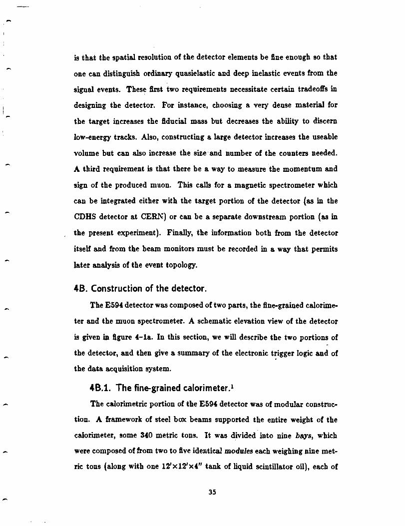
Figure 4-1. a. Elevation of the E594 detector .................. 36
b. ;Layout of an individual calorimeter module . . . . . . . . 36
4-2. HV pulse forming network . . . . . . . . . . . . . . . . . . . . . . . . 38
4-3. Flash chamber readout . . . . . . . . . . . . . . . . . . . . . . . . . . . 39
4-4. Proportional wire chamber . . . . . . . . . . . . . . . . . . . . . . . . 40
4-5. Proportional chamber integrating amplifier schematic .... 41
4~. Toroidal spectrometer magnets . . . . . . . . . . . . . . . . . . . . . 43
4-7. Toroid proportional wire chamber extrusion ............ 44
4-8. Secondary flux monitor systems . . . . . . . . . . . . . . . . . . . . 4 7
4-9. a. Layout of Fermilab . . . . . . . . . . . . . . . . . . . . . . . . . . 59
b. Neutrino area . . . . . . . . . . . . . . . . . . . . . . . . . . . . . 59
4-10. a. Neutrino energy-radius correlation .............. 66
b. Muon momentum-radius correlation . . . . . . . . . . . . 66
4-11. Resolution in neutrino energy versus cut location n ..... 67
Figure 5-1. Hits around vertex ("Pacman") cut .................. 70
5-2. Hits past vertex ( "QBOX") cut . . . . . . . . . . . . . . . . . . . . 73
S-3. Rejection percentages by filter cuts . . . . . . . . . . . . . . . . . . 77
S-4. Q2 distributions . . . . . . . . . . . . . . . . . . . . . . . . . . . . . . . . . 79
S-5. Monte Carlo signal and background Q2 distributions ... 80-81
5~. Rebinning scheme in Q2 • • • • • • • • • • • • • • • • • • • • • • • • • • 83
5-6. Rebinned differences, Q2 • • • • • • • • • • • • • • • • • • • • • • • • • 84
5-7. E B2 distributions . . . . . . . . . . . . . . . . . . . . . . . . . . . . . . . 88
S-8. Monte Carlo signal and background EB2 distributions .. 89-90
S-9. Rebinning scheme in EB2 • • • • • • • • • • • • • • • • • • • • • • • • • 91
S-9. Rebinned differences, EB2 • • • • • • • • • • • • • • • • • • • • • • • • • 92
5-10. 11 distributions . . . . . . . . . . . . . . . . . . . . . . . . . . . . . . . . 95
7

-
.-
l• . C.' ._ •
LIST OF FIGURES Po.ge
5-11. Monte Carlo 1J distributions .................... 96--97
5-14. Rebinning scheme in JI • • • • • • • • • • • • • • • • • • • • • • • • • • 98
5-15. 90% confidence limits on non-V-A parameters ...•..• 100
5-16. 68.5% confidence limits on left-right model parameters. . 104 Figure C-1. Garga111elle E02 /2me distribution . . . . . . . . . . . . . . . . . . 107
6-2. CHARM Q2 distributions . • . . . . . . . . . . . . . • . . • . • . . . 108
Figure C-1. Charge division network . . • . . . . . . . . . . . . . . . . . . . . . 122
C-2. ~ plot . . . . . . . . . . . . . . . . . . . . . . . . . . . . . . . . . . . . . 123
8

LIST OF TABLES
Table 3-1. Quantities constraining non-V-A couplings
3-2. Results to fits, {previous world average)
Page
. . . . . . . . . . . . 28
a. For fermion-mirror mixing models . . . . . . . . . . . . . . . 33
b. For left-right symmetric model . . . . . . . . . . . . . . . . . . 33
Table 4-1. Detector properties . . . . . . . . . . . . . . . . . . . . . . . . . . . . . . 36
4-2. Statistics for the 1982 narrow-band beam run . . . . . . . . . . . 61
4-3. Muon momentum resolution . . . . . . . . . . . . . . . . . . . . . . . . 62
4-3. Vertex resolution . . . . . . . . . . . . . . . . . . . . . . . . . . . . . . . . 64
Table 5-1. Electrons in fiducial volume ........................ 73
5-2. Events passing second stage of cuts . . . . . . . . . . . . . . . . . . 75
5-3. Obs~rved and expected low-Q2 excesses ............... 85
5-4. Acceptance of low-Q2 signal, number of neutrinos
on target, and integrated cross section . . . . . . . . . . . . . . 86
5-5. Observed and expected low-E82 excesses .............. 93
5-6. Fits to 11 distributions . . . . . . . . . . . . . . . . . . . . . . . . . . . . 99 5-7. Results to fits, (world average)
a. For fermion-mirror mixing models . . . . . . . . . . . . . . 102
b. For left-right symmetric model . . . . . . . . . . . . . . . . . 102
5-8. Contributions to x2 from each experimental constraint . . . 103
5-9. Results to fits, (this experiment only)
a. For fermion-mirror mixing models . . . . . . . . . . . . . . 105
b. For left-right symmetric model. . . . . . . . . . . . . . . . . 105
9

-
-
Chapter I. INTRODUCTION AND OVERVIEW.
The history of the attempts to understand the weak interaction is a long
one, and bas engaged quite a few of the greatest physicists of this century.
The properties of the weak interaction are peculiar to it alone among the
four fundamental interactions known in nature; such phenomena as parity
and CP violation are powerful limiting factors on the form a truly unified
theory of the physical world is allowed to take. In recent years, great advances
toward understanding the basic interactions have been made with the advent
of unified and grand unified gauge theories, and it is the task of experimental
and theoretical physicists alike to test these theories against observations.
In the particular case of neutrino interactions, it bas been clear since
1933 that spin degrees of freedom were important, when Pauli postulated an
unseen spin-t particle to ensure energy and angular momentum conservation
in nuclear beta decay.1 The next year, Fermi developed a theory of beta
decay based on a point-like interaction of four spin-l particles. 2 This was
soon generalized to encompass all weak interactions. In _19561 Yang and
Lee observed that there was no compelling theoretical reason for parity to
be conserved in the weak interactions,1 a conjecture that was subsequently
borne out by the experiments of Wu and others in 1957. To the present time,
the data have been consistent with a purely left-banded interaction among
leptons that is mediated by massive gauge bosons.
Theories that seek to explain the strong, the weak, and the electro-
10
-
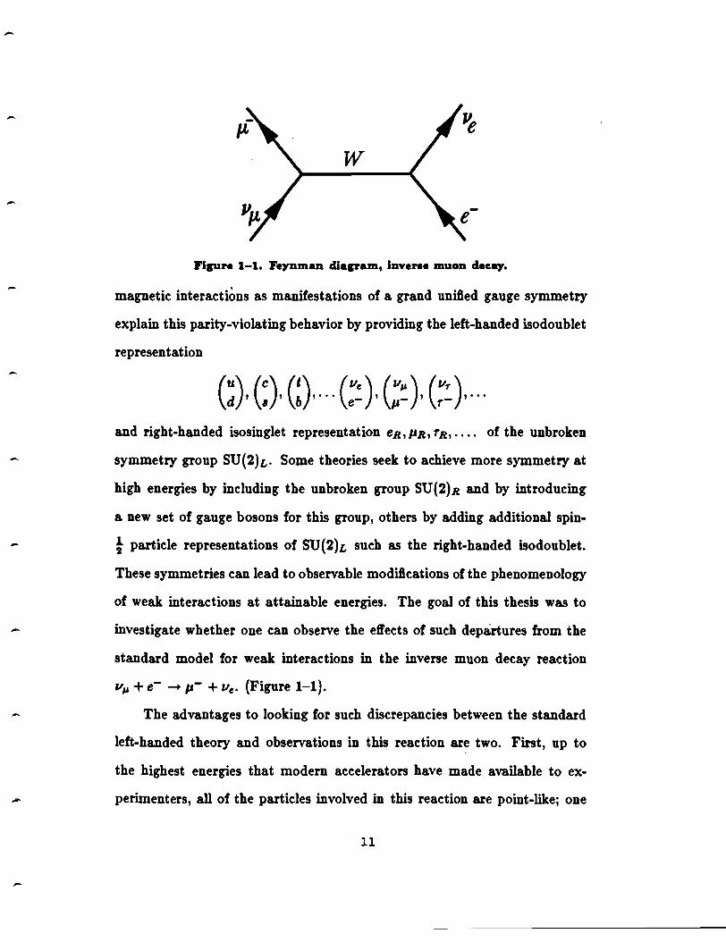
w
Figure 1-1. Feynman diagram, lnvene muon clecq.
magnetic interactions as manifestations of a grand unified gauge symmetry
explain this parity-violating behavior by providing the left-handed isodoublet
representation
and right-handed isosinglet representation eR, PR, rR,.... of the unbroken
symmetry group SU(2)L· Some theories seek to achieve more symmetry at
high energies by including the unbroken group SU(2)R and by introducing
a new set of gauge bosons for this group, others by adding additional spin
! particle representations of SU(2)L such as the right-handed isodoublet.
These symmetries can lead to observable modifications of the phenomenology
of weak interactions at attainable energies. The goal of this thesis was to
investigate whether one can observe the effects of such departures from the
standard model for weak interactions in the inverse muon decay reaction
Vµ + e- -+ µ- +Ve· (Figure 1-1).
The advantages to looking for such discrepancies between the standard
left-handed theory and observations in this reaction are two. First, up to
the highest energies that modern accelerators have made available to ex
perimenters, all of the particles involved in this reaction are point-like; one
11

-
-
-
need not worry about corrections that come from the less well understood
theory of strong interactions (to an excellent approximation). Second, exper
imental observation of the reaction is contaminated by only one significant
background, namely, the quasielastic scattering of neutrinos off' of nucleons
IIµ+ N - µ- + N'. (Figure 1-2). This can be distinguished from the sig
nal by comparing the data derived from a neutrino exposure, which contains
both signal and background, with those derived from an antineutrino ex
posure, which lacks the signal in the case of pure V-A. Also, among the
neutrino events, the presence of hadrons recoiling at the vertex disqualifies
an event from being an inverse muon decay. The main disadvantage to using
the inverse muon decay reaction is the same one that most neutrino experi
ments share-it is difficult to amass a large body of data on account of the
low cross-section.
We have performed a high-energy experiment in a narrow-band neutrino
beam at Fermilab with a massive, fine-grained, calorimetric detector. In this
thesis, we shall try to extract as much information as possible about the
chiral structure of the weak charged current using the data we have gathered
on the inverse muon decay reaction. To motivate this study, the essential
theoretical underpinnings will be surveyed in Chapter Il. The present state of
knowledge on the chiral structure of the weak interaction will be presented in
Chapter m, including results obtained by previous searches for inverse muon
decay in wide-band neutrino beams. A description of the E594 experiment
at Fermilab will follow ill Chapter IV, starting with a presentation of the
properties of the detector. This chapter will also contains a discussion of the
way the raw data from the experiment were analyzed by means of a computer
to give us the fundamental measurable quantities needed. In Chapter V
12

w
(•)
J,.Y
(b)
Figun 1-2. Feynman cllagram1, (a) Qua1lelaltlc neutrino-nucleon 1cattering, (b) Qua1lelaltlc antlneutrlno-nucleon 1catterlng.
the analysis of the data will be treated in detail and the two tests of the
standard V-A theory will be presented, along with their results. Finally,
the significance of these results will be discussed in Chapter VI, with a brief
apologia of the experimental procedure.
13

CHAPTER II. THEORY
2A. The weak interaction.
The original formulation of the weak interaction was constructed in
analogy with that of quantum electrodynamics. The Hamiltonian for the
nuclear beta decay process lacked the propagator factor of l/q2 , however,
which implied that the four fermions which participated in a reaction inter
acted at a single point in space-time. In accordance with Lorentz invariance,
the most general transition matrix term could contain bilinear combinations
(¢10it/12)(¢sOi(Ci + Ch5 )t/14 ) where Oi is one of the five operators
oi 1
1, (Scalar)
15 = ho"Y1"Y2"'f3 , (P seudoscalar)
1", (Vector)
"'(5"'(µ'
""J/ = th"' "'f 1/ 1'
(Axial vector)
(Tensor) .
¢ is the four component spinor representation of the fermion, and the "'f ma
trices are 'x' complex matrices from the Dirac theory. If time reversal
invariance is not assumed, each of the 10 coefficients Ci, c; may be com
plex, giving a total of 19 real undetermined constants (allowing for an overall
phase).1
In order to explain the nuclear beta decay reactions in which the nucleus
undergoes a spin-flip, the so-called Gamow-Teller transitions, purely vector
14
coupling is not sufficient in the weak matrix elements. Experiments that
measured the polarization of the outgoing leptons2•3 showed that the scalar
and axial vector terms would produce the wrong belicities if they predomi
nated. The pseudoscalar term would produce a very slight correction to the
matrix element and was neglected. In the end, a matrix element composed
of only vector and axial vector (V and A) terms was favored. Experiments4
showed that leptons were predominately left-banded (negative belicity) and
antileptons right-handed (positive belicity) and that the weak interactions
tended to violate parity maximally. These dictated a predominately "V -A"
form for the interaction:
.T. (1 -1s) .1, 'Ylp. 2 'Y
in which the matrix operator (1 -15 )/2 is the left-banded projection oper
ator. This form was applied to other weak interactions as well; one early
success was the prediction of branching ratios in the decay of pseudoscalar
mesons. This test of the V-A interaction and the others which have been
applied over the years will be discussed in Chapter m.
The theory was made renormalizable when, in the early 1970's, Glasbow,
Weinberg, 't Hooft and many others elucidated the non-Abelian gauge struc
ture of the electromagnetic and weak interactions combined. In this theory,
the V-A structure appears in the weak isospin group SU(2)L, where the "L"
stands for "left-banded". The weak interactions are mediated by spin-1 gauge
particles, thew= and zo bosons, which acquire a mass of about 100 GeV /c2
by the Higgs mechanism. In the present experiment, the effects of the prop
agator masses are entirely negligible on account of the relatively low energy
in the center of momentum frame (E* ~ 0.1 GeV). It is expected, however,
that the theoretical analysis would still be valid once the propagator masses
15

are taken into account.
28. Inverse muon decay.
The inverse muon decay reaction is a particularly convenient one to cal-
culate because of the pointlike structure of all the particles involved. It is
a cross channel of direct muon decay, which was characterized in the 1950's
in terms of the Michel parameters. It has the experimental advantage that
three out of the four leptons have known four-momenta. Furthermore, the
corresponding reaction for antineutrinos o" + e- -+ µ++lie would be strictly
forbidden if lepton numbers are conserved in an additive fashion.5 This sup
plied a "clean" sample of background quasielastic scattering events which
could be subtracted from the neutrino data (in the differential cross section
tests, sections 5B and SC) or which could be subjected to the same analysis as
the neutrino data to help distinguish the effects of actual signal from artifacts
of detector acceptance, background, and resolution. A detailed derivation of
the differential cross-section is too long to include here; the interested reader
is referred to Appendix A. The result of this derivation, allowing arbitrary V
and A couplings only, is:
• m [ ~+~ ] -d = _. F (1 - m!) (1 + P)(l - .\)y " 2 + (1 - P)(l + .\) 11 "1:11' 1 - m"
(2.1)
where P is the polarization of the incident neutrino beam, .\ gives the hand
edness of the coupling, 11 is the Lorentz invariant inelasticity (E11 - E11.)/ E11 ,
and 1 is the square of the energy in the center of momentum frame. In the
standard picture of left-handed two-component neutrinos and V-A coupling,
the parameters P and .\ take the values -1 and 1 respectively and there is
no II dependence in the cross section. This combination of parameters gives
the maximum value for the cross section integrated over g; if we set .\ = -1,
16
-
-
-
P = 1, (V +A with right-handed neutrinos) we obtain an integrated cross
section only about one-third as large. This allows an experiment that cannot
measure II directly (in a broad-band beam) to place limits on these parame-
ters.
An experiment that measures the integrated cross se,etion sets simulta
neous limits on P and .\ with one equation of constraint. Alternatively, one
may attempt to determine the handedness of the weak interaction (.\) ab
solutely, by estimating the amount of right-handed neutrino flux composing
the incident beam (P = zi~:~ ~ zi~~l ). If neutrinos have masses they
will have finite velocities /3 < 1 and helicities equal to -/3, and will appear
in both polarization states. These masses may be inserted as extensions to
the Glashow-Weinberg-Salam theory by adding terms to the Lagrangian of
the form
(2.2)
where mu is a unitary mass mixing matrix and l, l' are lepton spinors.
If l = l' then this is a Majorana mass term, otherwise it is a Dirac mass
term. A possible theoretical motivation for including this type of mass term
arises in the context of certain grand unified theories such as SO( 10) which
possess left-right symmetry.6 The helicity of the final state nuclei in spin-
0 nuclear beta decay Fermi transitions has been measured7 (and hence, by
angular momentum conservation, the helicity of the neutrinos) and the data
are consistent with. purely left-handed two-component neutrinos.
In broad-band experiments, it is necessary also to average over 1 in in
tegrating the cross section, since this quantity cannot be measured directly.
One resorts to modelling the beam energy distribution on computers. In
contrast, experiments in a narrow-band neutrino beam can measure the in-
17

-coming neutrino energy Ev and apply
(2.3)
to reduce the uncertainties introduced in such an approach. In principle, the
parameters P and ~ can be separated because one can measure 1J and flt
to the form of the difl'erential cross section, achieving one more equation of
constraint. In practice, problems with low statistics and with experimental
resolution limit the applicability of this method severely.
One of the unattained goals in the verification of the Glashow-Weinberg
Salam model is to flnd the Higgs particles. If charged Higgs particles can cou
ple to leptons, such as in certain extensions of the standard model, 8 scalar
or pseudoscalar currents may be observed in inverse muon decay. The inte
grated cross section for various combinations of arbitrary S, P, V, A, and T
couplings has been calculated for this reaction9 and is given in detail in
Appendix B. To obtain constraints on the parameters, data from the in
verse muon decay as measured by the CHARM collaboration were combined
with data from experiments measuring direct muon decay, pseudoscalar me
son decay, polarization of positive muons produced in inclusive antineutrino
reactions, and electron polarization in Gamow-Teller transitions. A total of
nine difl'erent models were investigated with difl'erent assumptions concerning
universality and which couplings to include. Each of these models used the
integrated cross section of the inverse muon decay to constrain the coupling
constants, although not all of the other data were used in each case. The au
thors of this study found that quite substantial departures from pure V-A
were consistent with experiment (up to 30%) owing primarily to the poor
agreement of the electron polarization data from direct muon decay experi
ments with theory.
18

-
-
-
2C. Quasielastic scattering of neutrinos.
The only significant experimental background to the inverse muon decay
reaction is quasielastic neutrino scattering 11µ+N<0> - µ-+N<+> where N<0>
is a neutron (or, possibly, a heavier neutral baryon) and NC+) is a proton
or some other positively charged baryon, such as the~+. (See figure l-2a)
There is also an analogous reaction of antineutrinos: IJ11 +NC+) -+ µ+ + N(o)
(figure l-2b). These reactions have been studied in great detail in the past
two decades of neutrino experim~nts as a way to probe the form factors of
the nucleon.10•11 Inverse muon decay can be distinguished from quasielastic
scattering in four ways. It is characterized by a muon produced at a small
angle to the neutrino beam, without extra tracks leading away from the
vertex. It is subject to a threshold for the incoming neutrino energy of
10.9 Ge V. Its Q2 distribution is very sharply peaked, covering only values
less than 0.2 Ge V2, as compared with the broad quasielastic Q2 distribution
out to 1.0 GeV2 and higher. (This is due to the low reaction mass of the
electron as compared to the nucleon.) The 11 distribution of inverse muon
decays is broad, because of the large amount of unseen energy in the final
state, whereas the same distribution for quasielastics is peaked at zero-
indeed, this may be taken to be the definition of a quasielastic scattering
event.
To simplify the formulation of the dynamics in quasielastic scattering,
time-reversal invariance, conserved vector current, lack of an induced pseu
doscalar term, and charge symmetry are usually assumed. This assumes that
no so-called "second-class currents" are involved. The results are expressed
in terms of dipole form factors for the axial and vector currents:
F1 ( ') _ F(O) V,A Q - (1 + Q2 /M~,A)' (2.4)
19
-
-
-
-
where MA, Mv are mass scales. By conservation of the vector current, Mv is
set equal to 0.84 Ge V to agree with electron scattering data. The most
recent weighted average value of MA is 1.03±0.04 GeV.11 This parameter
determines the shape of the Q2 distribution.
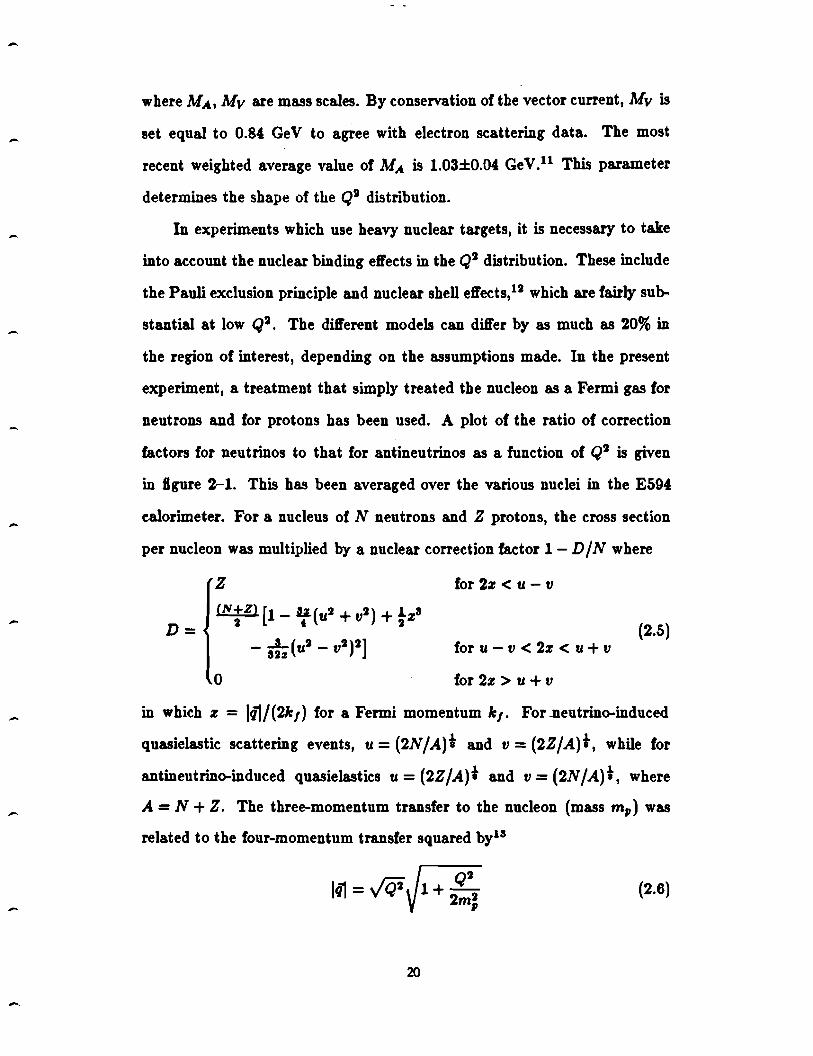
In experiments which use heavy nuclear targets, it is necessary to take
into account the nuclear binding effects in the Q2 distribution. These include
the Pauli exclusion principle and nuclear shell eff'ects,12 which are fairly sub
stantial at low Q2 • The diff'erent models can dift'er by as much as 20% in
the region of interest, depending on the assumptions made. In the present
experiment, a treatment that simply treated the nucleon as a Fermi gas for
neutrons and for protons has been used. A plot of the ratio of correction
factors for neutrinos to that for antineutrinos as a function of Q2 is given
in figure 2-1. This has been averaged over the various nuclei in the E594
calorimeter. For a nucleus of N neutrons and Z protons, the cross section
per nucleon was multiplied by a nuclear correction factor 1- D/N where
D=
z (N~Z> (1- ~(u2 + v2) + tzs
_ ~(u2 _ v2)2]
0
for 2z < u - v
(2.5) for u - v < 2z < u + v
for 2z > u + v
in which z = 141/(2k1) for a Fermi momentum k1. For.neutrino-induced
quasielastic scattering events, u = (2N/A)t and v = (2Z/A)t, while for
antineutrino-induced quasielastics u = {2Z/A)i and v = (2N /A)t, where
A= N + Z. The three-momentum transfer to the nucleon (mass m,) was
related to the four-momentum transfer squared by13
191 = /Qi J l+ Q' 2m2 ,,
20
(2.6)

-
•
• •
-CD
• Q .. .... ...... ac • I§ u
-N
.. -- •. 00 2 . a . 'l•os ' •JO r &,a . eo I . a
Figure 2-1. Ratio of nuclear correction factor• (neutrino• over antlneutrlnoa)
va. Q2 for quulelutlc acaUerlng.
In detectors with limited spatial resolution about the vertex there is also
the difficulty that processes such as single-pion production:
Vµ + n-+ µ- + n + 1r+
Vµ + n-+ µ- + p + 1rO
Vµ + p-+ µ- + p + ,,.+
may be misidentified as quasielastic events containing only a proton in the
final hadronic state. There is a large contribution to these processes through
the I= 3/2 (A) resonant channel and through a non-resonant I= 1/2 ftnal
state, 14•15 mainly at higher Q2 • In the present experiment, one relies on the
ability to subtract such a contamination from the signal in the integrated
cross section test (section SB) by using the antineutrino data. These have
the analogous reactions
IJµ + p -+ µ+ + n + 1ro
"" + p -+ µ+ + p+ ,,.-
21
-
-
-
tJ11 + n -+ µ+ + n + r-
which may lead to one or more tracks near the vertex. To get an unbiased
sample of quasielastic scattering events in the antineutrino data in this ex
periment, the restriction on finding tracks leading from the vertex (which
see, sections •C.5 and 5A.2e) was not imposed.
22
-
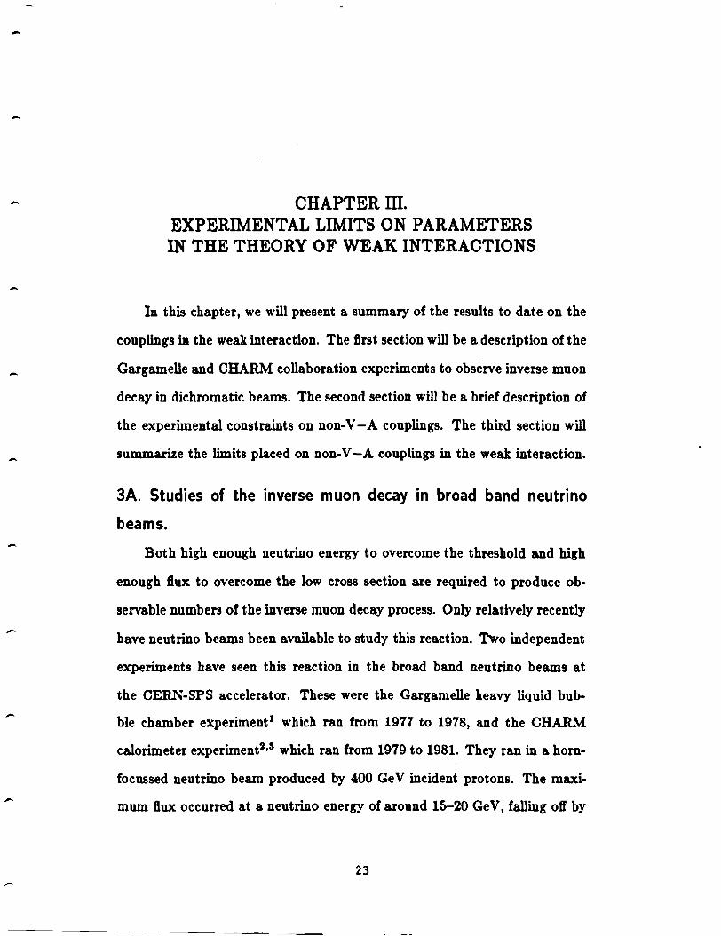
CHAPTER ill. EXPERIMENTAL LIMITS ON PARAMETERS IN THE THEORY OF WEAK INTERACTIONS
In this chapter, we will present a summary of the results to date on the
couplings in the weak interaction. The first section will be a description of the
Gargamelle and CHARM collaboration experiments to observe inverse muon
decay in dichromatic beams. The second section will be a brief description of
the experimental constraints on non-V -A couplings. The third section will
summarize the limits placed on non-V -A couplings in the weak interaction.
3A. Studies of the inverse muon decay in broad band neutrino
beams.
Both high enough neutrino energy to overcome the threshold and high
enough flux to overcome the low cross section are required to produce ob
servable numbers of the inverse muon decay process. Only relatively recently
have neutrino beams been available to study this reaction. Two independent
experiments have seen this reaction in the broad band neutrino beams at
the CERN-SPS accelerator. These were the Gargamelle heavy liquid bub
ble chamber experiment1 which ran from 1977 to 1978, and the CHARM
calorimeter experiment2•3 which ran from 1979 to 1981. They ran in a horn
focussed neutrino beam produced by 400 Ge V incident protons. The maxi
mum flux occurred at a neutrino energy of around 15-20 Ge V, falling oft' by
23

"' . 0
'; li ,.
Figure 1-1. CERN-SPS neutrino flux. (Ref. l)
one order of magnitude by 50 GeV. (See Figure 3-1). The Ve contamination
of the Vµ beam was estimated3 to be 11 %. The construction and running
conditions of these two experiments will now be described briefly, postponing
the discussion of the results until chapter 6.
The Gargamelle experiment (which is depicted in Figure 3-2) used a
mixture of propane (C3H8 ) and freon (CF3Br) as a target with mean density
0.51 g/ml. The visible volume was 7.2 m3 , which contained a fiducial volume
of 4.01 m3 and a 8.ducial mass of one metric ton. A muon track was detected
by means of a pair of multiwire proportional chambers placed upstream and
downstream of the chamber (the upstream chamber acted as a veto) and an
external muon identifter (EMI) made up of two sets of proportional chambers
24
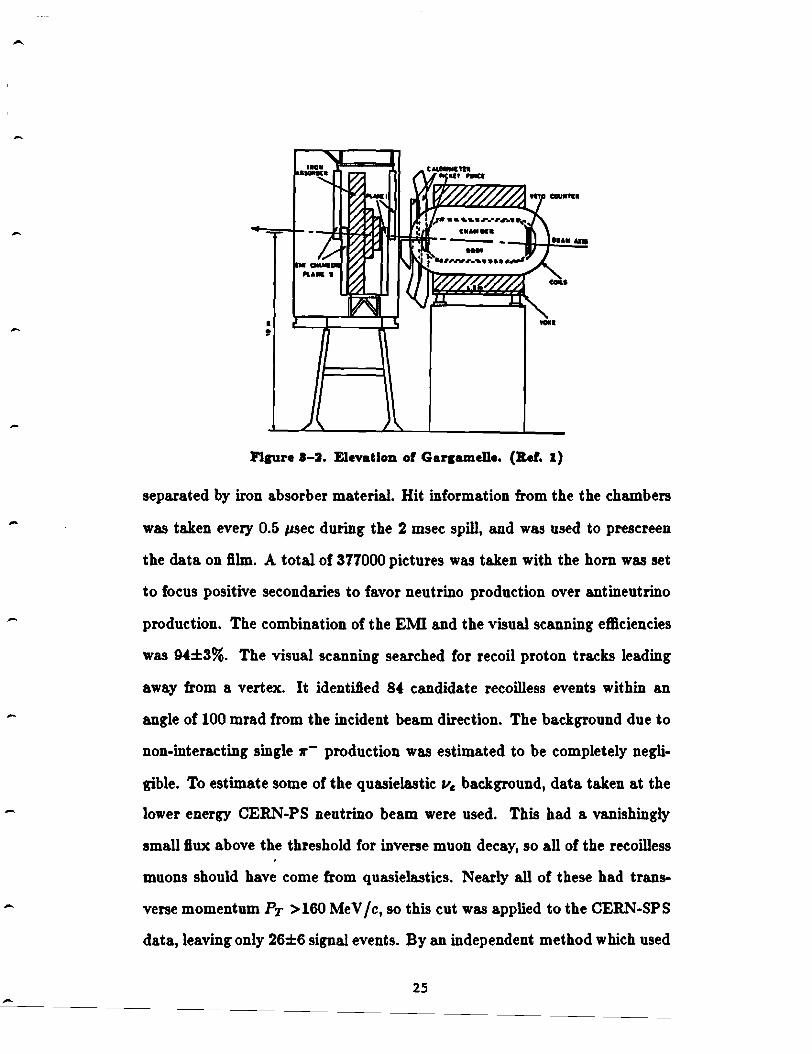
-
-
I ,
l'Jgure 1-2. Elevation of Gargamelle. (Ref. 1)
separated by iron absorber material. Hit information from the the chambers
was taken every 0.5 µsec during the 2 msec spill, and was used to prescreen
the data on fllm. A total of 377000 pictures was taken with the horn was set
to focus positive secondaries to favor neutrino production over antineutrino
production. The combination of the EMI and the visual scanning efficiencies
was 94±3%. The visual scanning searched for recoil proton tracks leading
away from a vertex. It identi1ied 84 candidate recoilless events within an
angle of 100 mrad from the incident beam direction. The background due to
non-interacting single 1r- production was estimated to be completely negli
gible. To estimate some of the quasielastic 11, background, data taken at the
lower energy CERN-PS neutrino beam were used. This had a vanishingly
small flux above the threshold for inverse muon decay, so all of the recoilless
muons should have come from quasielastics. Nearly all of these had trans
verse momentum Pr >160 MeV /c, so this cut was applied to the CERN-SPS
data, leaving only 26±6 signal events. By an independent method which used
25

-
-
Figure 1-1. View of the CHARM detedor.
the distribution of the candidate events in E11 and 6: for inverse muon decay
signal and for background, the experimenters arrived at the same number of
signal events.
The CHARM detector4 (see Figure 3-3) used marble slabs for target ma
terial. The cross sectional area presented to the beam was 3m x 3m. This area
was surrounded by a frame of magnetized iron and was instrumented with
layers of plastic scintillation counters and of proportional drift tubes. A total
of 1560scintillators and 13000drift tubes (including the toroid chambers) was
used. The main calorimeter was followed by a toroidally magnetized muon
spectrometer consisting of an end calorimeter and three end magnets. These
were instrumented with drift tubes, which could measure the track coordi
nates with 1 mm resolution. The event trigger was defined by the coincidence
of four scintillator plane hits, a minimum of 50 Me V detected ionization, and
a track that traversed the spectrometer. After cutting on muon polarity,
and on lack of visible energy about the event vertex, there was a total of
. 26

-
-
1684:3 neutrino events. Of these, 937 had Q2 < 0.02 GeV and p" >10 GeV.
The background from quasielastic scattering was estimated from the shape
of the antineutrino data plotted in Q2 ; it accounted for 551±36 of the events,
leaving an excess of 386±36. This was corrected for detector acceptance and
for selection efficiencies to give a total corrected number of inverse muon
decays of 594:±56(statistical)±22(systematic) events. Under the conditions
of the experiment, the V-A theory with left-handed neutrinos would have
predicted about 606 events.
3B. Experimental constraints on non-V-A couplings.
Table 3-1 lists the experimental quantities, other than the inverse muon
decay cross section, which place constraints on the deviations from V-A in
the context of various alternative models of the weak interaction. We will
give a brief description of each of the quantities, leaving a fuller description
to the references in the literature5•6•7 from which this section is adapted.
38.1. Leptonic charged current.
These quantities are measured in four types of experiment. The first
type looked at the ratio of pseudoscalar meson (pion and kaon) decay to
electrons and to muons, R,,(K). The best values for R.,, and RK were mea
sured by Di Capua et al.8 and by the CERN-Heidelberg collaboration.9
These have been normalized by the V-A values R!'-A = 1.230 x lo-• and
Rk-A = 2.4:74: x lQ-5 • The second type measured the longitudinal polariza
tion of the muon, Pµ, from pion decay.10 The third type looked at -(c/v)PtJ-,
the polarization of electrons produced in nuclear beta decay. The most cur
rent estimate for this is given by Koks and van Klinken. 11 Finally, the direct
muon decay process, µ - evµVe, has been characterized by nine parameters:
spectrum shape (p, q), asymmetry((, 6), electron helicity (h), and transverse
27

) ) ) ) ) ) )
Table 1-1
Quamltl .. c:omtralnlng non-V-A. c:oupllnp
Quantity· Measured V-A value Units Ref. R,,,/Jl';-A 1.023±0.019 1 8
Pµ 0.99±0.16 1 10 RK/R~-A 0.978±0.044 1 9 -(c/u)P~- 1.001±0.008 1 11
p 0. 7517±0.0026 0.75 13 PµE 0.975±0.015 1 13, 14
6 0. 750±0.004 0.75 20 h 1.008±0.054 1 15
(tr( Vee)) 7.6±2.2 5.586 10-46 cm2 7 tr(Vµe)/ E11 1.54±0.67 1.376 10-42 cm2 /GeV 7
N tr(vµe)/ E11 1.46±0.24 1.503 lo-42 cm2 /GeV 7 00 tr(v11e)/tr(t>µe) 137+0.65 1.092 7 • -0.44
AFB 11.8±3.9 7.57 % 7 hvv 0.009±0.040 0.0048 7 R- 0.264±0.008 0.261 7 R+ 0.315±0.009 0.325 7 R, 0.47±0.064 0.401 7 Rn 0.22±0.031 0.240 7 a1 -9.7± 2.6 -6.64 10-5Gev-2 7 at 4.9 ± 8.1 -6.23 10-5Gev-2 7 B -1.40 ± 0.35 -1.37 10-4Gev-2 7
PµE6/p 0.9989 ± 0.0023 1 19
-
-
electron polarization (a, (J, a', (J'). Of these, p, 6, h, and PµE are useful in
constraining the non-V -A couplings. These quantities have been measured
by various experiments, as indicated by table 3-1.
3B.2. Leptonic neutral currents.
By using data from the neutral current weak interactions, one can elim
inate certain ambiguities in the parameters of a model. 7 Among the purely
leptonic processes, we can use three sets of data to set limits on the cou
plings. These are the total cross section for fiee scattering averaged over the
beam spectrum, (D'(fiee)), and the total cross sections for fiµe and 11µ.e scat
tering, D'{fiee) and D'(vee). We also use hvv, the coefficient of {l + cos2 8)
for e+e- -+ µ+ µ-, as well as the associated parameter of forward-backward
asymmetry AF 8 , but since the published formulae for these quantities do not
seem to agree with the flt values our results will differ from those of the pre
vious studies. The experimental input for hvv was measured at PETRA,16
and the value for AF 8 at J'i = 33.5 Ge V has been measured by Bartel et
aI.17
3B.3. Semileptonic processes.
When we consider the weak interactions of quarks, we need to make
certain assumptions about the ways in which the quarks can participate in .
non-V-A couplings.' To suppress flavor changing neutral currents via the
GIM mechanism, in the context of a fermion-mirror fermion mixing model,
we must assume that the quark-mirror quark mixing angles are negligible.7
With this assumption, we may set constraints on the model by looking at
the ratios of total cross sections:
R* = D'Nc(vµ~) ± D'Nc{fi11~) D'cc(11µN} ± D'cc(fiµN)
29
(3.1)
-
-
-
.-
-
for isoscalar targets N and
(3.2)
for nucleons N = p, n. These were measured by a number of experiments,
as quoted in reference 7. The additional constraints provided by the data
on charge asymmetry in polarized lepton-hadron scattering (parameters a1,
a:.1, and B) disagree by a constant factor between the flt values of reference 7
and the formulae given both there and in other references.18 We will adopt
these formulae and compute the expected values without comparing to the
published flt.
3C. Present limits on non-V-A couplings.
We considered possible deviations from the standard V-A couplings in
the framework of three possible models. The most general model, which
introduced various amounts of S, T, and P couplings in addition to the stan
dard V and A couplings, was discussed by Mursula et al. 6 Since we have
been unable to reproduce the derivations of the formula for the inverse muon
decay cross section (section BC of appendix B) for the present experimental
conditions, this model was not analyzed fully here. Instead the two other
hypotheses, which admitted only vector and axial-vecto:i;: couplings in the
charged weak interaction, were investigated in some detail. These were the .
fermioa-mirror fermioa mixiag model, inspired by such models as SO(n > 10)
and SU(n > 5), and the left-right symmetric model, which was based on the
flavor group SU(2)LxSU(2)RxU(l).
The fermion-mirror fermion mixing model combined the conventional
left-handed doublet (~) L and right-handed singlet representations lii, '1R of the weak isospin group SU(2)L with corresponding right-handed doublet
30

-
-and left-handed singlet representations (?) R ,li., ViL to make up the lep
tonic mass eigenstates of fermions and mirror fermions. The gauge particles
were unchanged. The predictions of such a theory depended on the relation
of the masses of the mirror fermions to those of the conventional fermions.
References 5 and 7 considered six distinct cases in analyzing the experimen
tal results (see appendix B for details). The adjustable parameters were the
mixing angles for charged leptons flt and for neutrinos t/>t, which would all
be zero for the V-A limit.
The left-right symmetric model5•12 introduced gauge bosons WR of the
gauge group SU(2).R. These would mix with the conventional left-handed
gauge bosons W L, through spontaneous symmetry breaking, to form mass
eigenstates. The adjustable parameters were the mass ratio of the two gauge
bosons mw L / mw R and the mixing angle w. In the V -A limit,mw L / mw R = 0
and w = 0. Also, as the center of mass energy increased, the effect of the
(heavy) WR bosons would increase and non-V-A behavior would become
more apparent.
Table 3-2a gives the results of our fits to the experimental data for
several different cases of the fermion-mirror fermion model. The quanti
ties constraining the fits were the leptonic charged current measurements of
p, 6, PµE, h, R,,, RK, P11 , P/J-, and the integrated cross section for inverse
muon decay, S (excluding the result of the present experiment), the neutral
current measurements of (o-(Vee)), o-(vµe), and o-(v11 e), and the semileptonic
quantities R,, R,., R+, and R-. The goodness-of-flt quantity x2 was mini
mized for these quantities simultaneously after having combined the values
of h and PtJ- and of R,, and RK by weighted means. The integrated cross
section for the inverse muon decay has a different dependence on the mixing
31

-
-
-
angles for each of the cases (for details on this dependence, see appendix B).
Table 3-2b gives the results of flts to the experimental data for the left
right symmetric model. The quantities p, Pµ(, h, R,,, RK, Pµ, P~-, and the
integrated cross section for inverse muon decay, S, (excluding present results)
were used in the x2 minimization process, with R.,, and RK being combined
beforehand. See appendix B for details on how the integrated cross section
of inverse muon decay depended on the two parameters of the theory.
In chapter 5, we will return to these two types of models and re-evaluate
the couplings with the value for the inverse muon decay cross section that
this experiment was able to obtain. It should be noted, for future reference,
that of all the experimental inputs we consider, only one, the longitudinal
polarization of the electron in muon decay (Pµe), deviated appreciably from
the pure V -A value.
32

) )
Model 9e 9em1u
&coh 1.1 2.0
8inc free* free hcoh 1.1 1.8 hioc free free c 5.0 13.3 dcoh 0.0 38.2f dine free free
)
Table 8-2a B.eaulh lio flh for fermion-mirror fermion modela
(value for S from CHARM experiment) Be•t flt• and ea.a" C.L. value•
"'~ tJJ~ma.:i 9µ (JIJma~ t/Jµ
8.5 16.5 0.0 2.3 8.9 6.5 15.9 free free 7.7
16.0 25.0 0.0 3.8 0.0 15.9 25.0 free free 0.0 14.0 18.8 2.5 9.2 13.9 4.4 7.1 0.0 1.6 9.0 4.3 7.1 free free 7.9
•unconatralned paramelier f Parabollc error e•tlmate
All value• In degtee•. Pure V -A give• •ero for all mixing angle•.
Table l-2b L•ulli• to flt for the left-right •ymmetrlc model
(value for S from CHARM experiment)
Quantity Fit value
0.14 0.0°
68.3% C.L.
0.18 1.9°
x2 = 3.0 for 5 degree~ of freedom. Pure V-A vBlue I• •ero for eada parameter.
)
t/Jµmas sin2 Ow x2 /d.f.
- 13.6 0.249 9.4/18 12.2 0.247 9.9/18 44.9f 0.24() 10.2/16 4.1 0.240 10.6/18
18.2 0.22l 8.3/16 13.6 0.249 9.9/16 12.3 0.246 9.9/18
! .

CHAPTER IV. THE E594 EXPERIMENT AT FERMILAB.
In this chapter, we will try to give a description of the parts of the
E594 experiment that played maJor roles in the observation of inverse muon
decay. Section 4A is a brief statement of objectives we wished to reach.
Section 4B gives a description of the physical configuration of the apparatus,
including the electronics and the beam monitors. Section 4C is a description
of the computer routines which were used in the analysis of the data, and
which played as important a role in this experiment as the hardware itself.
Section ID summarizes the running conditions for this experiment, including
a description of the generation of the dichromatic neutrino beam. The final
section, 4E, discusses the way in which the response of the detector and of
the analysis routines to neutrino-induced events was calibrated.
4A. Considerations in the choice of detector properties.
A successful counter-based neutrino detector must have a number of
properties to be able to record and to analyze inverse muon decay events. The
first requirement is that the instrumented volume comprise a large mass. This
is especially important in a narrow-band neutrino beam which has a lower fiux
of neutrinos than a wide-band horn focussed beam. The second requirement
34
-
-
is that the spatial resolution of the detector elements be fine enough so that
one can distinguish ordinary quasielastic and deep inelastic events from the
signal events. These first two requirements necessitate certain tradeoff's in
designing the detector. For instance, choosing a very dense material for
the target increases the fiducial mass but decreases the ability to discern
low-energy tracks. Also, constructing a large detector increases the useable
volume but can also increase the size· and number of the counters needed.
A third requirement is that there be a way to measure the momentum and
sign of the produced muon. This calls for a magnetic spectrometer which
can be integrated either with the target portion of the detector (as in the
CDHS detector at CERN) or can be a separate downstream portion (as in
the present experiment). Finally, the information both from the detector
itself and from the beam monitors must be recorded in a way that permits
later analysis of the event topology.
48. Construction of the detector.
The E594 detector was composed of two parts, the fine-grained calorime
ter and the muon spectrometer. A schematic elevation view of the detector
is given in figure 4-la. In this section, we will describe the two portions of
the detector, and then give a summary of the electronic trigger logic and of
the data acquisition system.
48.1. The fine-grained calorimeter.1
The calorimetric portion of the E594 detector was of modular construc
tion. A framework of steel box beams supported the entire weight of the
calorimeter, some 340 metric tons. It was d_ivided into nine bays, which
were composed of from two to five identical modules each weighing nine met
ric tons (along with one 12'xl2'x4" tank of liquid scintillator oil), each of
35
-
'-
-
~~~~ IRON 12'TOROIOS
IRON 24' TOROIDS Flsure 4-la. El•vatlon of th• d•t•dor.
. I . . ~· I ...
~ .. .. I . .
Fleur• 4-lb. Layout of an lncilvldual calorimeter modul•
Detector properties
Tabl• 4-1
Length of calorimeter Cross section of calorimeter Total mass Density Radiation length (Xo) Absorption length (.\) Length in absorption lengths Mean atomic number
19.6 m 12'xl2' (3.7 mx3.7 m)
3.4 x 10⁵ kg 1.4 g cm-a
12cm 83 cm (116 g cm-2 )
22 .\ 21
which was composed of one proportional chamber plus four beams of four
flash chambers interleaved with four absorber planes. The structure of an
36

-individual module is depicted in figure 4-lb. The detector planes were sup
ported in a way that allowed easy access to the instrumentation; individual
planes could be removed for servicing. In all, there were 608 flash chambers,
37 proportional chambers, nine liquid scintillators, and 608 absorber planes.
Some of the properties of the overall detector are given in table 4-1. The
individual elements that make up the calorimeter are described in detail in
the sections which follow.
4B.1a. The flash chambers.
Flub chambers are devices which combine fairly good spatial resolu
tion with low cost and ease of fabrication. They are similar to spark chambers
in configuration, but are triggered externally and are segmented by insulat
ing walls within which the plasma discharge propagates. Each flash chamber
was constructed of three panels of extruded polypropylene that had cells of
rectangular cross section. The panels were taped edge to edge parallel to
the cells and aluminum foil was laminated to the two faces of the plane to
provide high voltage and ground electrodes 12' x 14'in size. A plane had a
capacitance of 30 nf. There were approximately 4x10⁵ cells in the entire
detector, 635 cells per flash chamber, with each cell 5 mm thick, 5.8 mm
wide, and 3.6 m long. The walls of the cells were about 0.5 mm in thickness.
The flash chambers were supplied continuously with a miXture of 96% Ne,
4% He, 0.17% Ar, 0.10% H20, and 0.04% 0 2 and N2 by means of a mani
fold along one edge; the gas was collected at the opposite edge, purified in
molecular sieves, and recirculated at the rate of approximately one volume
change per hour. This mixture of gases had been chosen after much research
into combining the minimimum reflre probability of the chambers with the
maximum efficiency.
37

-
I_ SQ
FLASH CHAMBER +HV
39nf 30nf !Onf
0.4JJ.h
GAP Figure 4-3. BV pulae forming network.
When the trigger logic detected an event, a high voltage pulse was sent
to the electrodes of each flash chamber by a pulse forming network (PFN)
approximately 700 nsec after the event (see figure 4-2). This 4.5 kV peak
voltage pulse had a 60 nsec rise time and a 500 nsec duration, and was
monitored to insure uniformity in timing, pulse height, and pulse shape. As
we shall see in the description of the proportional wire chambers, the RF
noise generated by this surge of current was a formidable constraint on the
design of readout systems.
The strong electric field between the electrodes caused rapid avalanche
multiplication of any ionization left by charged particles that had traversed
the gas in a flash chamber cell. This resulted in a plasma which expanded
towards the ends of the chamber at a speed of about 0.1 ft nsec-1 • At
one end of a chamber, the plasma discharge was capacitively coupled to a
3 mm wide copper readout strip which connected to ground. (See figure 4-
3). The 0.5 A current spike induced on this copper strip in turn induced an
acoustic pulse on a 0.005" x0.012" magnetostrictive wire contained in a wand
38
I Mil

I_
-
-
SIDE VIEW OF READOUT
....,,,...., .... ., Q--(C.la ............... .
Figure 4-1. Fla•h chamber readout.
assembly which ran across the flash chamber cells and which was maintained
at a constant magnetization. The acoustic pulse then propagated with low
dispersion toward the two ends of the wire at about 5000 m sec-1 or 1 µsec
per cell. Along with the pulses from the chambers, three fiducial markers at
known positions along the wand were provided. The pulses were detected and
amplified and the information from the timing of the pulse trains from each
end yielded a unique pattern of hit cells on the chamber. The clock period
used for timing the pulses corresponded to just under half a cell width and
had been chosen in order to reduce problems caused by bad synchronization
and by variations in cell width.
The information given by a flash chamber was simply whether one or
more charged particles had traversed a given cell somewhere along its length,
for the nature of the plasma process eliminated any pulse height or particle
counting capability. To measure track coordinates in two dimensions, three
sets of chambers were used with cells oriented horizontally (the X chambers
39

-,_
)_
-
-
-
illustrated in figure 4-lb) and at approximately ±10° from the vertical (the
U and Y chambers) to provide stereo views of an event. There were 304
X chambers and 152 each of U and Y chambers.
4B.1b. The proportional wire chambers.
Prompt information from a neutrino interaction within the detector was
gathered with a system of proportional wire chambera that traversed the
detector, one per module, to make trigger decisions. In addition, pulse height
information on charged particles passing through these chambers was gath
ered, allowing a cross-calibration of the flash chambers' response to energy
deposited by particles to the proportional tubes' response. The pattern of
hits was latched and stored to give a useful starting point when analyzing
the data off-line in determining the boundaries of each event and in deciding
whether a given set of hits recorded by the flash chambers was in fact due to
an event in time with the event trigger.
Flsun 4-4.. Proportional win chamber.
The proportional wire chambers (figure 4-4) were constructed of ex
truded aluminum sections 12' ( 3.6 m) in length in the shape of eight rect-
40

-
-
fOlll' WUH
-I -I -I
--i
lnt•~ator
1Y/pC
tut o~t 250 nHC cllp
pln •'
600 n .. c d•l9.1'
elo• out pin• z.5
Figure 4-1. Proportional daamber lntiegrailng amplifier adaemaHe.
angular cells with inner dimensions 0.840"x0.910" (2.13 cm x 2.31 cm).
Eighteen aluminum extrusions placed edge to edge made up a single 144 wire
plane. There were 5300 wires in the entire calorimeter. To provide two views
of an event, vertical cells and horizontal cells altemated in successive mod
ules. There was a gold plated tungsten anode wire strung down the middle of
each cell, 50 µm in diameter. This was supported at each end by a pin passing
through a nylon bolt which made a gas seal in the walls of an aluminum gas
manifold. The gas mixture was 90% Ar-10% CH4 (P-10), and was supplied
at 0.5 ft9 hr-1 or one volume change per day, without recirculation.
A positive voltage of 1600V was applied to the anode wire to give a gas
gain of approximately 3000. The negative-going signal pulse passed through
a blocking capacitor to the input of an FET integrating amplifier which had
a gain of 1 V /pC. (See figure 4-5.) There were 1300 amplifier channels in
the calorimeter. Four adjacent tubes shared a common amplifier channel to
provide 411 (10.2 cm) spatial resolution. A monolithic 600 nsec tapped delay
line differentiated the signal to form the fast-out signal which was passed
along coaxial cable to the trigger electronics, discriminators, and ADC units.
Also, a track and hold system of CMOS switches allowed the signal pulse to
41
-
-
...
-
charge up a capacitor which was read out much later over twisted-pair cables
to give pulse height information (the slow-out signal). To insure integrity of
this stored charge during the time when the flash chambers PFNs generated
their high voltage pulse, these switches and the signal lines that controlled
them had to be protected against transients and the capacitors were selected
specifically for their low leakage rate. Tests of the chamber response with and
without the flash chambers triggering indicated that .these were sufllciently
protected against noise. Small Cd109 sources mounted directly over the cells
allowed calibration of pulse height response between event triggers, so that
any variation of the gain with the pressure of the gas or the applied voltage
could be detected.2
4B.1c. Absorber planes.
The major contribution to the mass of the detector was in the absorber
planes. They provided both a target for the neutrinos and a medium for
the development of hadronic and electromagnetic showers. In this exper
iment the absorber material was constructed of hollow acrylic extrusions
filled with either sand or steel shot. Each flash chamber was sandwiched be
tween one sand plane and one shot plane. This yielded an average sampling
distance of 3%.-\ = 22%X0 for the flash chambers and 50%.-\ = 350%X0 for
the proportional chambers. The heavy atoms composing the absorber planes
constituted a target which was close to isoscalar.
48.2. The muon spectrometer.
The other major portion of the E594 detector was the system of bend
ing magnets and proportional wire chambers downstream of the calorimeter
to measure the momenta of energetic muons produced in charged current
neutrino interactions. This momentum could then be combined with the
42
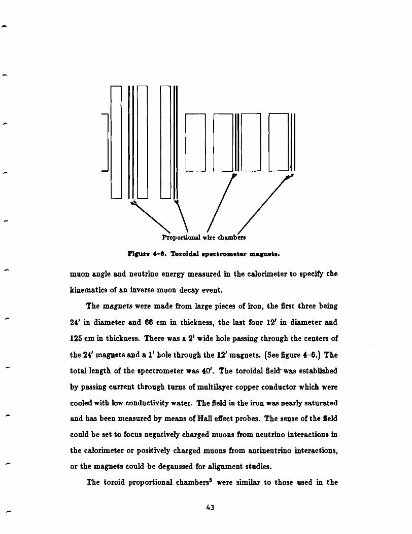
-
-
-
-
-
-
~\ Proportional wire chamben
Figure 4-45. Toroidal •pedrometer mapet•·
muon angle and neutrino energy measured in the calorimeter to specify the
kinematics of an inverse muon decay event.
The magnets were made from large pieces of iron, the first three being
2•' in diameter and 66 cm in thickness, the last four 12' in diameter and
125 cm in thickness. There was a 2' wide hole passing through the centers of
the 2•' magnets and a 11 hole through the 12' magnets. (See figure 4-6.) The
total length of the spectrometer was 40'. The toroidal field· was established
by passing current through turns of multilayer copper conductor which were
cooled with low conductivity water. The fleld in the iron was nearly saturated
and has been measured by means of Hall effect probes. The sense of the B.eld
could be set to focus negatively charged muons from neutrino interactions in
the calorimeter or positively charged muons from antineutrino interactions,
or the magnets could be degaussed for alignment studies.
The toroid proportional chambers3 were similar to those used in the
43
-
-
calorimeter, but with some important differences. To achieve the required
momentum resolution, one needed 0.5" ( 1.3 cm) resolution in the sagitta
of each muon track coordinate. The following changes to the calorimeter
proportional chambers were required. First, instead of using eight cell single
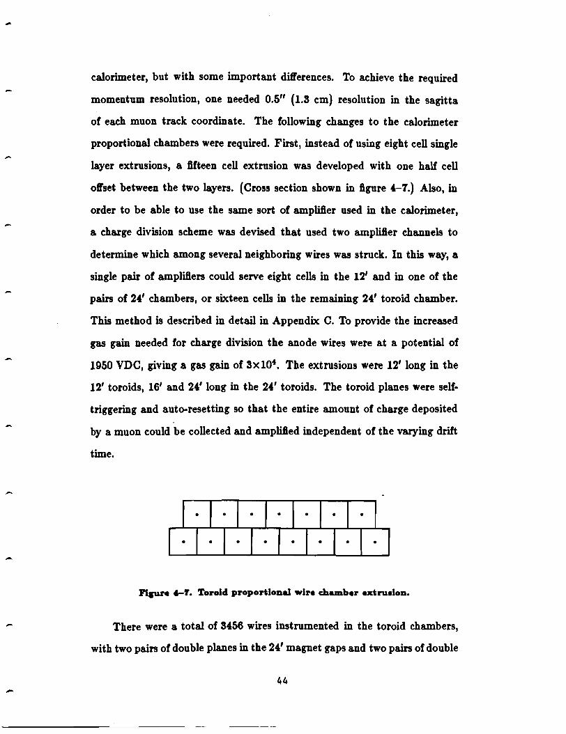
layer extrusions, a 6.fteen cell extrusion was developed with one half cell
offset between the two layers. (Cross section shown in 6.gure 4-7.) Also, in
order to be able to use the same sort of amplifier used in the calorimeter,
a charge division scheme was devised that used two amplifier channels to
determine which among several neighboring wires was struck. In this way, a
single pair of amplifiers could serve eight cells in the 12' and in one of the
pairs of 24' chambers, or sixteen cells in the remaining 24' toroid chamber.
This method is described in detail in Appendix C. To provide the increased
gas gain needed for charge division the anode wires were at a potential of
1950 VDC, giving a gas gain of 3xl04• The extrusions were 12' long in the
12' toroids, 16' and 24' long in the 24' toroids. The toroid planes were self
triggering and auto-resetting so that the entire amount of charge deposited
by a muon could be collected and amplified independent of the varying drift
time.
• • • • • • •
• • • • • • • •
Flpre 4-f. Toroid proportional wire chamber extru•lon.
There were a total of 3456 wires instrumented in the toroid chambers,
with two pairs of double planes in the 24' magnet gaps and two pairs of double
44

-
,_
I_
-
-
-
-
planes in the 12' gaps. Each pair consisted of a plane of vertical wires and a
plane of horizontal wires. The same gas mixture used in the calorimeter was
supplied to the toroid chambers, 90% Ar-10% CH4 , at about 1 ft3 hr-1 •
48.3. The trigger logic.
The prompt information from the calorimeter and toroid proportional
chambers and the liquid scintillators could be combined in a great number of
ways to create specialized triggers for particular applications. This section
will first catalogue the elements that made up a particular trigger, then
describe the two triggers used in gathering inverse muon decay data.
The fast-out signals made by differentiating the integrating amplifier
output from each of the 36 channels in a plane were processed with fast elec
tronics on the plane to provide several output signals. An analogue summing
circuit on the "Sum and Multiplex" board added up all the fast-outs on that
plane to make a sum-out signal E. On the "Electron Logic Board" the
individual fast-outs were discriminated with a 20 m V threshold to form the
bit bit NIM level logic signal for each amplifier channel. An analogue signal
with height equal to 60 m V times the number of hits bits set on a plane was
also generated; this was the analog multlpllclty signal AM.
These fast signals were sent through 500 coaxial cables to a second stage .
of logic residing in NIM standard bins. Cable lengths were adjusted so that
the signals from different planes would arrive at the logic simultaneously.
The sum-out signals were added linearly to give a total pulse height or sum
sum signal EE to measure total energy deposited. To form the pre-trigger
condition M, the sum-outs were discriminated with a threshold of 50 mV; if
the signals from two or more planes exceeded this, M was generated. The
analog multiplicities were discriminated and the N condition was satisfied if
45

-
, _ I
I ,_
-
-
-
-
more than some preset fixed number of these were above a preset threshold.
All of the digital signals were latched for later analysis and all of the analogue
signals were sent to peak-sensing ADC units and stored.
The two triggers used to collect inverse muon decay data were the Quasi
trigger and the PTHtrigger. The Quasi trigger required that there be hits in
the front and back planes of the muon spectrometer, that EE correspond to
no more than 10 Ge V deposited in the calorimeter, and that there be no hit
in the upstream scintillator veto counter. This trigger was designed to cut
out any large hadronic or electromagnetic shower events in the calorimeter,
events where the muon exited the toroid region before reaching the end, and
through muon events. The PTH trigger was a low bias trigger formed by the
coincidence of the following trigger elements:
M > 2 planes
EE> 75 mV
N > 1 channel in > 1 plane
Front scintillator veto.
Since an average muon passing through the calorimeter deposited 5 GeV
of energy, some of the inverse muon events did satisfy this energy deposition
requirement, along with some of the quasielastic events. For both neutral
and charged current deep inelastic events, this trigger was essentially 100%
eftlcient down to 5 Ge V shower energy, with a drop in efficiency below this
energy.
48.4. Beam monitoring and control.
The calculation of the expected number of inverse muon decays depended
upon the estimation of the number of neutrinos that passed through the
fiducial volume. In this section, we will describe the system for monitoring
46
-
-
··~
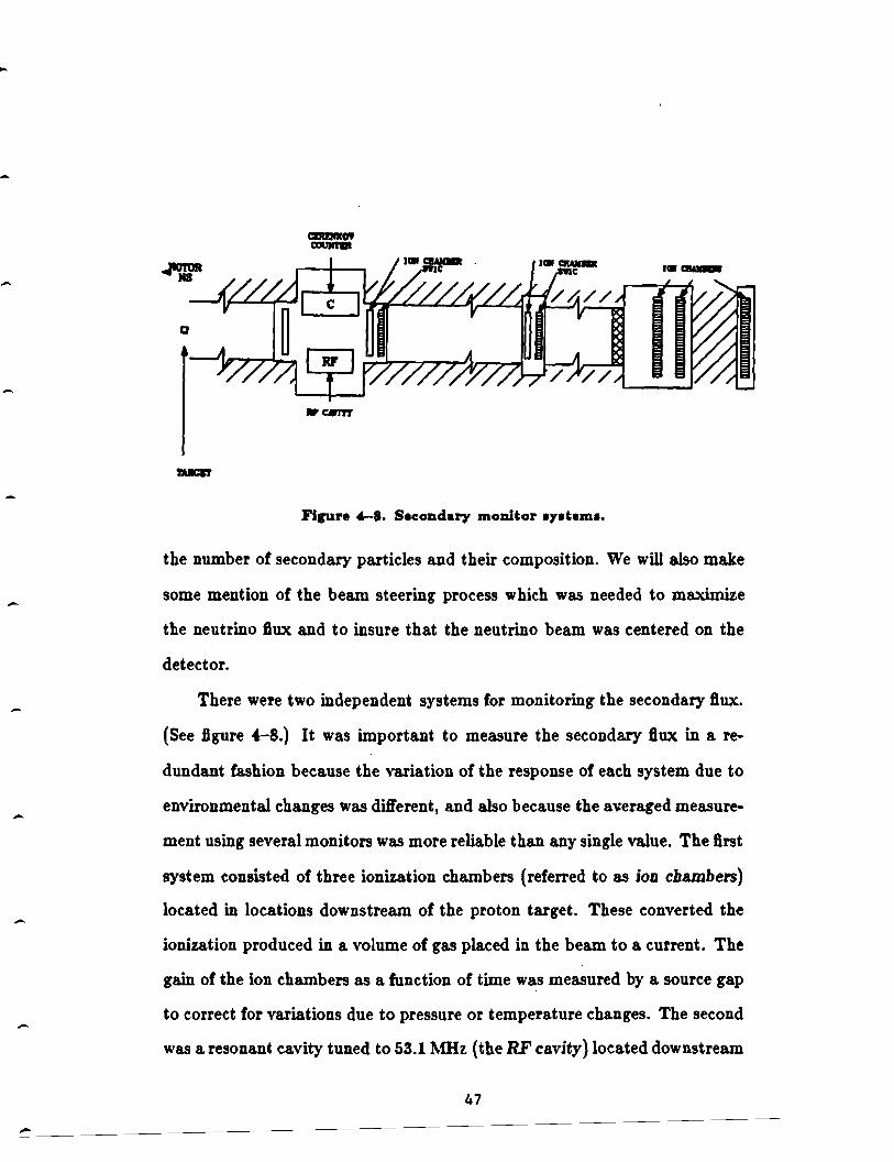
Flgur. 4-8. Second&!')' monitor •y•hm•.
the number of secondary particles and their composition. We will also make
some mention of the beam steering process which was needed to maximize
the neutrino flux and to insure that the neutrino beam was centered on the
detector.
There were two independent systems for monitoring the secondary flux.
(See figure 4-8.) It was important to measure the secondary flux in a re
dundant fashion because the variation of the response of each system due to
environmental changes was different, and also because the averaged measure
ment using several monitors was more reliable than any single value. The Brst
system consisted of three ionization chambers (referred to as ion chambers)
located in locations downstream of the proton target. These converted the
ionization produced in a volume of gas placed in the beam to a current. The
gain of the ion chambers as a function of time was measured by a source gap
to correct for variations due to pressure or temperature changes. The second
was a resonant cavity tuned to 53.1 MHz (the RF cavity) located downstream
47
-
-
of the first ion chamber. This produced a voltage pulse in response to the
beam 8.ux. The output pulses of each of these systems were converted to a
frequency and scaled to produce digital data which were recorded on mag
netic tape. Each of the digitizers was calibrated with known pulses between
spills to make sure that its performance was stable. The output of each de
vice was integrated for up to six diff'erent several time periods or "gates" so
that not only the total number of neutrinos could be determined but also the
number that was incident during the live time of the detectors on the neu
trino beam line. The master beam gate was synchronized with the passage
of the -iOO GeV proton beam which was detected by a toroidal pickup.
To give an absolute reference for the beam 8.ux, the output of the RF
cavity and of the ion chambers was compared to the observed amount of 24Na
produced in a 0.005" thick copper foil by 200 GeV protons. For this reaction,
the activation cross section is known to within about 3%. Conections to this
calibration were made for the diff'ering response of the ion chambers to proton
and meson beams and for the eff'ect of the diff'erent spill shapes in the foil
activation and the neutrino runs on the RF cavity response.
The composition of the secondary beam was measured by a helium dif
ferential Cerenkov counter which could be introduced into the beam in place
of the RF cavity. This counter had a fixed annular iris, ind the counting
rate as a function of pressure re8.ected the amount of each successive charged
species making up the beam. The particle fractions thus determined provided
a constraint on the simulation of the beam transport which was performed on
the Cyber computers. This simulation took the known settings of the train
magnets and their geometry and returned a spectrum of particle momenta
and spatial distribution at the end of the magnet train, before the particles
48
-
-
-
reached the decay region. Another computer simulation could then relate
these results to an expected neutrino energy and flux at the Lab C detector.
The beam position was monitored by means of a system of split plate
multiwire ion chambers. This measured the amount of beam passing on the
two sides of a horizontal or vertical boundary to determine the degree of ver
tical or horizontal mis-steering of the beam respectively. The experimenters
would be alerted when this became too great, so that the magnet currents
could be corrected. All of the split plate ion chamber outputs, as well as the
digitized values of the magnet currents, were recorded on tape.
The systematic error in the neutrino flux contributed to the error in the
expected number of inverse muon decay events (see sections SB and SC). The
estimated error of about S% is small compared to the statistical error in the
observed number of events for any of the cross section tests we have used.
48.5. Data acquisition.
The large size and 6.ne granularity of the detector along with the rela
tively high noise environment made the task of data acquisition and storage
a major task in this experiment. A typical neutrino event involved thousands
or tens of thousands of pieces of flash chamber information as well as pro
portional tube, scintillator, calibration, and beam monitor information, all
of which had to be recorded, packed, and written to magnetic tape.
The flash chambers and proportional chambers were read out using
CAMAC compatible crates using 24 bit words. The calorimeter and toroid
proportional chambers were addressed separately using separate levels of data
multiplexing on the planes themselves and remotely. The data was packed
into custom-made CAMAC compatible memory units which were then read
onto temporary disk storage by way of block transfers. Flash chamber HV
49
-
,_
-
..
pulse quality information was gathered by an LSI 11/23 processor with asso
ciated memory which then filled CAMAC memory for transfer to the main
computer. Monitor information was gathered for the main computer by the
MAC system, which also allowed the experimenters to control portions of the
beam line. The main computer was a PDP 11/45 that wrote the data onto
800 bpi tape, displayed views of the incoming data on screens in the control
room, computed certain statistics for the use of the experimenters to verify
that everything was running properly, alerted them when an alarm condition
did occur, and did a certain amount of fast data analysis.
4C. Off-line analysis.
In this section we will describe the major parts of the data analysis
which were used in the study of inverse muon decay. These include the
muon tracking package, the vertex finding routines for quasielastic candidate
events, Monte Carlo simulations of the physics of the inverse muon decay
and quasielastic scattering processes and of the response of the detector, and
data handling routines. Detailed information concerning the software used in
the studies of the integrated signal cross section and of the diJl'erential cross
section are contained in the next chapter where these studies are described.
Measures of the performance of several of the routines which were relevant
to this thesis are discussed in section 4E below. All of the off-line analysis
was written in FORTRAN and run on the Control Data Cyber 175 and 875
computer cluster at Fermilab.
The raw tapes written from the CAMAC units by the data acquisition
computer contained the data in a form that was easy to store but hard to read
out in a sensible fashion. To solve this problem, a preliminary stage of data
handling called reformatting was needed; this condensed the data, subtracted
50

-
1-
-
the pedestals from proportional chamber data and the offsets from fiducial
marks in flash chamber data, and repackaged each record separately from
the others in an orderly arrangement of planes and channels. This simplified
the analysis of the data by a large amount and reduced the number of data
tapes needed. Only certain rather specialized applications ever needed to use
the raw tape information. The analysis routines which are described below
all read the data from reformatted tapes.
4C.1. The muon vertex finding routines.
When an event had been identified as a potential inverse muon decay
candidate, the vertex routines were called to find the location of the primary
interaction and the angle of the muon at this point. The position of the ver
tex was combined with our know ledge of the dichromatic beam to estimate
the energy of the interacting neutrino (see section 4C.4 below on how this
was done) and was one necessary input to the muon tracking package (sec
tion 4C.2). The location of the interaction was also needed to show where to
look for energy that had been deposited by recoil nucleons, nuclear fragments,
or other final state hadrons in a quasielastic or low-y inelastic event. The
quality of the muon vertex finding procedure and of its applications in this
experiment is an illustration of the advantages of good pattern recognition
properties in a fine-grained calorimeter.
Only isolated hits were considered within the calorimeter at first; hits
that seemed to be associated with many other hits were disregarded tem
porarily (by using the subroutine CNTRST). Starting at the end of the
calorimeter, the process would begin by searching for a string of isolated
hits that lined up. The angle and intercept of this track candidate would
then define the axis of a limited region or "road" within which the rest of the
51
-
,_
-
-
candidate muon track could be expected to lie. At this time the hits that had
been neglected before by CNTRST were once again taken into consideration.
A search for a series of chambers, in any view, containing no hits inside the
road would then begin, starting at the end of the calorimeter and proceeding
upstream. This location was taken to approximate the longitudinal position
of the vertex, with the lateral position given by extrapolating the angle of the
track candidate back from the end of the calorimeter. The hits in the vicinity
of the vertex would then be fitted via a least-squares method to a straight
line in order to refine the slope estimate. Finally, a second search from the
end of the calorimeter back to the vertex region for a series of chambers with
missing hits would then be performed, using a narrower road.
This approach to finding the interaction vertex through software had
the great virtues of reproducibility and speed, which recommend it over the
process of visual scanning, with which it in fact agreed quite well. The
resolution of the vertex position is discussed in section 4E.2 below.
4C.2. The muon tracking package.
Once a starting point and angle for a muon had been found, the track
could then be associated with hits in the toroid proportional chambers. One
could then determine the particle's energy by measuring the amount of bend
ing that occured in the magnetic field. The muon trackihg package was a
least-squares fitting algorithm in several unknowns that analyzed the ob
served hits, estimated the muon momentum on the basis of the known mag
netic field and amount of multiple scattering in the various parts of the
detector, and assigned an error in the momentum measurement by using the
covariance matrix. It had to be able to cope with the presence of noise hits
in the toroid chambers or in the calorimeter. It also depended intimately
52

-
-
on accurate surveying of the two parts of the detector separately and with
respect with one another.
The muon tracking process proceeded in two passes, the flrst using both
flash chamber information and toroid chamber information, the second using
only flash chamber information. The first pass considered hits in the rear of
the calorimeter and flt them to a straight line via least squares. Only hits
falling within a road of constant width around the estimated muon track
were considered in the calorimeter. Toroid hits were matched on the two
sides of the double planes, and were flt to various possibilities for a single
track consistent with the known magnetic field. The track candidate and
combination of hits which minimized the goodness of flt quantity x2 /d./.
(chi-squared per degree of freedom) was chosen. To help eliminate random
noise hits, the first pass through the data was performed in two iterations, the
second one omitting the one hit that made the largest contribution to x2 /d./.
for the best track candidate. The final set of hits for the flrst pass were used
as input for the second pass. This pass flt the hits near the estimated vertex
using the same road. In assigning a momentum to the muon, allowance was
made for d.E/dx of the particle through the calorimeter.
The muon tracking package retumed the sign and momentum of the
muon, the estimate of the error of this measurement, the x' /d./. and number
of degrees of freedom, and improved estimates of both the track slopes and
the errors in these slopes. If an event failed the analysis for any reason, the
package was able to communicate the reason for failure to the main program
and to tabulate the various failure modes. For debugging purposes, it was
possible to print out the results of intermediate steps in the fitting procedure
and to vary the values of parameters the package used.
53

-
4C.3. The Monte Carlo simulation.
Some aspects of the detector's response to neutrinos were simply impos
sible to deduce analytically. These included the eft'ect of noise, the efficiency
of the pattern recognition routines, the effect of misalignment on the exper
imental resolutions, and the smearing of the 11 and Q2 distributions by the
non-Gaussian tails of the resolution. Such effects were investigated by turn
ing to Monte Carlo simulations which would take the best estimates of the
kinematics of the particles involved in a reaction, combine these with the
best understanding of the physics of the interaction of particles with mat
ter, with magnetic fields, and with detector elements, then simulate the data
acquisition process to make data files of fictitious events. These could then
be analyzed with the same software used to analyze the real data and the
measurements could be compared with the true quantities.
The Monte Carlo package used to simulate the E594 detector was an
intricate piece of programming, reflecting in part the complexity of the ap
paratus. At the same time, since it had many users, each with a dift'erent goal
in mind, it was designed to be both flexible and easy for a user io operate
without much knowledge of its internal operations. At its heart was a list
of particles that were generated in the course of an interaction from nuclear
and electromagnetic interactions in the absorber medium,·from decays, and
from the primary vertex. These were propagated relativistically through the
detector, made to interact with nuclei in the absorber planes so as to cre
ate more particles or to be stopped, decayed, lost energy through ionization,
or generated electromagnetic showers. All these processes were modelled
with the same lifetimes and ranges that numerous other experiments have
measured. 4 The geometry of the detector was included in virtually every de-
54
-
,_ tail, the magnetic field in the toroid magnets was modelled, and the diff'erent
materials that made up the detector were included realistically.
To allow for a reasonable execution speed, a few concessions were made:
low energy ( <10 MeV) neutrons were ignored, strange particles were not pro
duced, electromagnetic showers were treated by means of a formula for energy
deposition rather than as a particle multiplication process, noise was put into
the 8.ash chambers in a uniform random way (aside from known "hotspots"
and "dead regions" which were included) rather than in the somewhat clus
tered way it appeared to occur, the trigger conditions were not explicitly
made use of in event generation, and the question of noise in the propor
tional tubes was largely ignored. On the whole, however, these refinements
have been studied and have been found not to make very much diff'erence in
the 8.nal appearance of the events or in the results of most types of analysis.
Every attempt to optimize the code has been made, with the result that only
about 0.25 seconds of CPU time was needed to generate a single quasielas
tic or inverse muon decay event. Finally, the response of the detector to
calibration beams of hadrons, electrons, and muons has been compared to
the results from analyzing Monte Carlo simulated data and, even though the
simulation does not itself make use of the calibration results, the responses
agreed very well. 5
4C.4. Neutrino energy determination.
Most applications of the E594 detector to physics in the narrow-band
beam required that the incoming neutrino energy be determined to help fix
the kinematics of whatever reaction is under study. The way this was done
was to use the kinematics of the decay of the secondary pseudoscalar mesons
which had been focussed and monitored in the secondary beam line and the
55
geometry of the beam line itself to deftne a correlation between the radial
position of a neutrino in the detector and its energy.
Since there were two types of pseudoscalar meson produced that could
give rise to neutrinos, pions and kaons, the relationship between radius and
energy was not one-to-one and it was in fact this aspect that gave the dichro
matic beam its name. At a given radius, furthermore, neither the pion band
nor the kaon band was perfectly monochromatic either, due to the non
negligible length of the decay region as compared with the distance from the
decay region to the detector, and also to the 8.nite momentum bite of the
train. There was also contamination from relatively rare decays (such as the
pion to electron-neutrino and the three-body kaon to muon-neutrino decays),
from wrong sign mesons that would enter the decay region, and from wide
band background neutrinos that resulted from decays of particles which had
not passed through the train. To take all of these effects into account, a
Monte Carlo simulation of the beam transport process was done using the
detailed information on the train and on the secondary beam itself and this
generated a series of 8.les that contained the distributions of neutrino energies
and types at many different radii from the center of the beam. To use this
information when analyzing the true data or when simulating the beam, the
neutrino energy package approximated the energy distribution from a given
decay mode by two gaussian distributions (one for pion-and one for kaon
band neutrinos) and to interpolate their values between diff'erent radii. The
value of the distributions at their peaks were used in calculations requiring
the neutrino energy using the information from the muon energy to decide
whether to use the pion- or the kaon-band value. The performance of the
neutrino energy measurement for inverse muon decay events is evaluated in
56
-
-
section 4E.3 below.
4C.5. Utility routines.
There were a great number of miscellaneous routines that made the
analysis and debugging of the analysis of neutrino events much easier. The
pictures of events that appear in this paper are products of a general event
displaying routine and of a graphical output package. There were routines
that would read the monitor information that was recorded along with the
information from the detector and could compute the number of secondaries
that are produced and the number of neutrinos passing through the fiducial
volume. Routines that enabled the creation of summary flies of kinematic
and topological quantities extracted from events allowed easy reanalysis of the
data. There were also routines that created alignment, efficiency, and pulse
height tables from source calibration and cosmic ray data. Finally, there
were the histogramming and data presentation packages HBOOK, HPLOT,
and DIGS, which produced most of the plots included in this thesis.
40. The 1981 and 1982 data collection runs.
There have been two periods of neutrino running and of calibration. The
results reported in this thesis came exclusively from the dichromatic beam
run and calibration in 1982, so only a brief summary of the 1981 wide band
engineering run and calibration will be given here.
The 1981 run comprised several weeks in May-June 1980 for calibration
and six months of neutrino running from January to June 1981. The calibra
tion running included exposures to electrons, hadrons, and muons at known
energies and angles. The neutrinos were generated by a wide-band hom fo
cussing beamline with 80 kA current through the hom. The decay distance
was 349 m. This beam consisted of neutrinos that were very strongly peaked
57
at low energy, and a flux of antineutrinos an order of magnitude less at most
energies. The detector weighed 240 tons total, with 416 flash chambers, and
21 calorimeter proportional chambers. The 24' toroid proportional chambers
had not been installed, and the 12' toroid chambers were not present for the
calibration beam. Various triggers and combinations of triggers were tested,
including a low bias energy deposition trigger, an electron trigger, a high Q2
trigger, and a quasielastic event trigger.
The 1982 ~n began in January 1982 with neutrino running at various
magnet train settings until May, when six weeks of hadron, electron, and
muon calibration beam was taken. After this, two weeks of running with the
beam collimator closed was taken in order to measure the wide-band back
ground, then studies on cosmic rays were done with the beam off'. During
periods when the accelerator was operating well, there were up to 1.2xl012
protons on target producing about 109 muon neutrinos in each spill through
the fiducial volume of the detector. This gave a total neutrino exposure
of about 5xl018 for the whole run (table 5-4). The train was set to fo
cus 100, 140, 165, 200, and 250 GeV /c positively charged particles for the
neutrino exposures and 165 GeV /c negatively charged particles (denoted by
"-165" in this thesis) for the antineutrino exposure. The +100 and +140
train settings had low numbers of events and peaked at relatively low neutrino
energy, so they were not used in the inverse muon decay study.
A diagram of the layout of the Fermilab site and of the neutrino beamline
is shown in figure 4-9. Neutral hydrogen atoms which were converted to H
ions and accelerated in a 750 keV Cockroft-Walton generator, which would
feed the 200 Me V linear accelerator after stripping the ions down to bare
protons. After this stage, the protons were accelerated in bunches by the
58
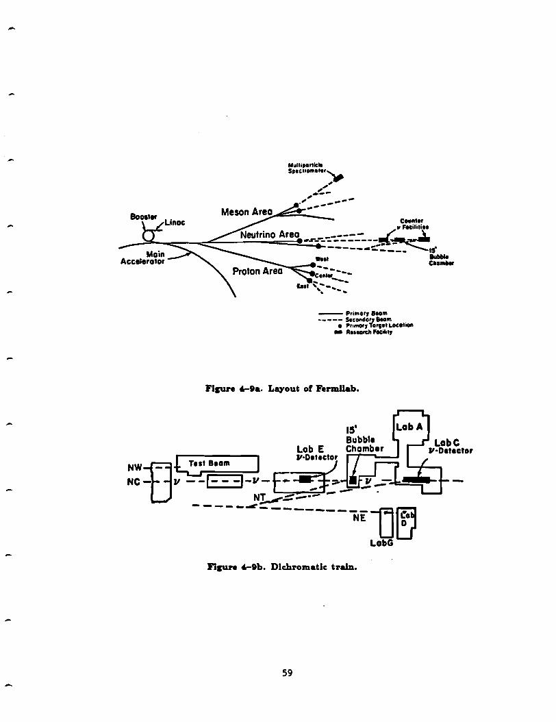
-
·particle Multi ••••-..... ...... Spu••- _r
, ,, ,, -·- -,, --·" -----
Primarr ';:".,. ~ S.cD11darr •tLocotioll -- - Promar1 Tarv
• rel! Ftlc:illlJ
Lll)'out o Flsure '-9•·
- R•HO
f Fermllab.
Lob E lf·Datactor
Q:;· ..... I r::-=< 1! ~ NWTI +--1-11-~..:'-NC LJ" ------..!'~~=_:.:. ___ NE1J1~·~
l train. Dlchromat c Flsun '-lb.
59
LabG

-
8 Ge V booster synchotron, which served as the injector stage to the main ring,
a proton synchotron. Here the protons achieved 400 Ge V after many turns
around the ring; at which time they were routed to the proton switchyard.
The beam was divided into three components which were sent to the Meson,
the Pro.ton, and the Neutrino beam areas. The absolute normalization of the
proton intensity delivered onto the beryllium oxide target in the Neutrino
area was done by interposing a piece of copper foil in the beam, which would
then be analyzed by nuclear chemical techniques to measure the dose (see
section 4B.4). The pions and kaons that were produced in the target were
focussed and transported down a train of magnets which could select the
desired momentum up to 250 Ge V / c. The beam was steered by controlling
the current settings of the train magnets via the MAC system. The mesons
decayed in flight by the reactions r --+ µ1111 , K --+ µ11,_., and K--+ r 0 µ11µ in
an evacuated decay region. The neutrinos which resulted from these decays
would then traverse 1 km of earth which would stop the hadrons that have
not decayed as well as the produced muons. The E594 detector was housed
in Lab C after the end of this earth shield.
The detector was essentially complete at the time of the run, and the
trigger conditions reached more or less their final form as well. Due to the
lower neutrino fluxes in the narrow band, the detector was operated on a
100% live basis for both the PTH and the Quasi trigger. If a beam spill
passed with neither of these trigger conditions fulfilled, the detector was
allowed to trigger on cosmic rays using the liquid scintillators, for alignment
and debugging purposes. A few differences from the 1981 calibration run
in the flash chamber HV pulse amplitude and timing made corrections in
the measured shower energy necessary prior to comparison. There was a
60

problem in the triggering hardware for the toroid chambers which degraded
the spectrometer data for the early part of the runj these runs have been
ignored in the present analysis.
A summary of important information concerning the 1982 narrow-band
beam run appears in table '-2.
Table 4-2
Statl•tlc. for the 1182 narrow-band beam rma
Number of neutrinos in fiducial volume 8x10¹³
Number of triggers taken
165 GeV:
200 GeV:
250 GeV:
-165 GeV: Primary proton energy
Mean neutrino energy (165 GeV train)
4E. Detector performance.
28,662
11,620 29,278
33,0,0
'00 GeV 55GeV
In this section the response of the detector and of the analysis ro~tines
is compared to the expected response. The expected response can sometimes
come from calibration, but often one must rely on Mont~ Carlo simulation
to provide such quantities as angular and vertex resolutions.
4E.1. Calibration muon beam.
The best way to measure the energy and angle resolutions of inverse
muon decay events was to use a calibration muon beam with a known en
ergy and angle and to compare the software results to the true values. The
calibration beam was made up of secondary particles produced by focussing
the primary proton beam on a target. These consisted of electrons, mesons,
61

-
-
-
protons, and muons. All except for the muons were filtered out by inserting
pieces of polyethylene ahead of the bending magnets which defined the mo
mentum. Plastic scintillator hodoscopes in coincidence with a "halo" veto
( 1nade of plastic scintillation counters positioned off to the sides of the beam)
provided the trigger. A problem that one encountered was that since the cal
ibration beam could not uniformly illuminate the detector at all angles and
positions, it was necessary to make certain that the portion of the calorime
ter that was illuminated by the calibration beam was representative of the
whole. The muon calibration beam covered a very small cross sectional area
as it traversed the calorimeter, but, since different momenta had different
amounts of bending in the spectrometer, different parts of the toroid cham
bers were illuminated at a given beam angle. Some events were taken with
the beam defining hodoscopes displaced so that the muons would enter the
detector at a different angle.
Tabl• 4-&. Muon mom•ntum n1olutlon. (Ref. t)
Po P(measured) u(P) P/Po u(P/Po)
22.3 22.9 1.8 1.03 0.08 44.0 4-i.1 -i.1 1.00 0.09 76.8 14.6 8.3 0.97 0.11
108.5 103.1 12.1 0.95 0.11 Po wu tih• untral momentum Httlng of &he calibration b•m All momuit;a ID Ge V
Data were taken at four energies from 22 to 109 GeV (see table 4-3).
It was found that the x2 / d./. returned by the muon tracking package was
rather sensitive to the range of Bash chambers selected in which to perform
the angular flt. This has been interpreted as indicating that the error in the
magnetic field was small compared with the error in Bash chamber alignment.
62
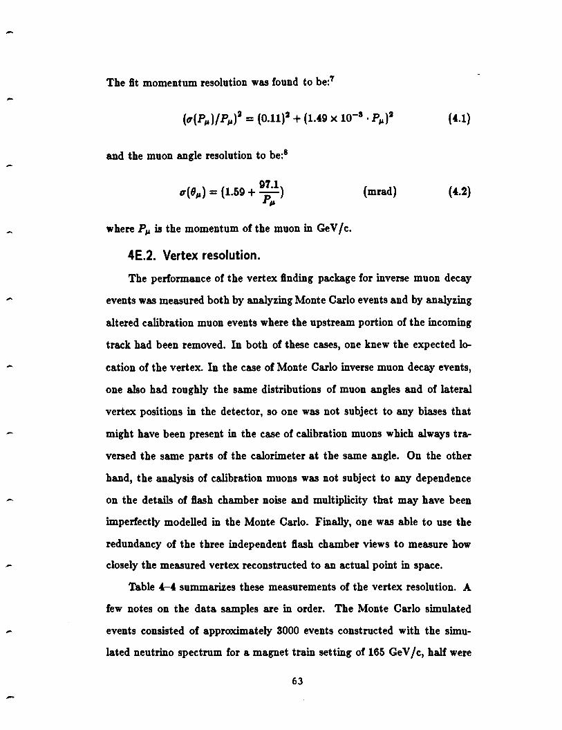
-
-
-
-
-
-
The flt momentum resolution was found to be:1
(u{P,.,)/P,S' = {0.11)2 + (1.49 x 10⁻³ • P,.,)2
and the muon angle resolution to be:8
u(B,.,) = (1.59 + 9;·1)
"' (mrad)
where P"' is the momentum of the muon in Ge V / c.
4E.2. Vertex resolution.
The performance of the vertex finding package for inverse muon decay
events was measured both by analyzing Monte Carlo events and by analyzing
altered calibration muon events where the upstream portion of the incoming
track had been removed. In both of these cases, one knew the expected lo
cation of the vertex. In the case of Monte Carlo inverse muon decay events,
one also had roughly the same distributions of muon angles and of lateral
vertex positions in the detector, so one was not subject to any biases that
might have been present in the case of calibration muons which always tra
versed the same parts of the calorimeter at the same angle. On the other
hand, the analysis of calibration muons was not subject to any dependence
on the details of flash chamber noise and multiplicity that may have been
imperfectly modelled in the Monte Carlo. Finally, one was able to use the
redundancy of the three independent flash chamber views to measure how
closely the measured vertex reconstructed to an actual point in space.
Table 4-4 summarizes these measurements of the vertex resolution. A
few notes on the data samples are in order. The Monte Carlo simulated
events consisted of approximately 3000 events constructed with the simu
lated neutrino spectrum for a magnet train setting of 165 GeV /c, half were
63

-
-
-
Table 4-4
Vertex reaolutlon
Data set !l.il. x z 6 2 (cm) (cm) (cm) (cm)
Muons, bay 2 9 4.5 18 13 bay 3 8 4.8 3 12 bay 4 9 5.4 9 17
Monte Carlo, V-A 4.0 2.6 1.9 2.2 V+A 5.6 3.1 2.0 2.6
generated with a pure V-A interaction assumed and half with pure V+A.
The calibration muon beam events had the hits within a narrow road around
either side of the incoming track removed. The road extended from the be
ginning of the detector to the middle of the second, third, or fourth bay as
indicated in the table. Muon energies were 22 and 108 GeV. As for the last
column in the table, the quantity
6 = u - II - 2 tan s.J/ ( Zo - z)
is the deviation from the ideal matching of the three views. Here, u, z, and 11
are the coordinates of the vertex in the U, X, and Y chamber views, z0 is the
off'set of the X chamber wands, and B.11 ~ 10° is the experimentally measured
inclination of the U and Y chambers from vertical. If 6 = O, the three views
for an event reconstructed to a single point in space (whether or not this
point was indeed the true interaction vertex). The standard deviation of 6
from zero wu a measurement of the lateral vertex resolution. We achieved
reuonably good performance of the vertex package, although the Monte
Carlo resolution outperformed the calibration muon resolution. This may
have been due to residual uncertainties in the flash chamber alignment, or
mistakes in eliminating the upstream muon hits. For . the purposes of the
present study, the vertex resolution wu adequate both from the point of
64

-
,_
-
-
-
-
view of determining the neutrino energy from its radial position, and for
defining regions where hadronic energy from inelastic scattering events may
be found.
4E.3. Neutrino energy resolution.
To accumulate enough events to study inverse muon decay effectively, it
was desirable to make the fiducial volume as large as possible when analyzing
the data. This volume intercepted a beam that was made of mixed pion-band
and kaon-band neutrinos. To estimate the neutrino energy, one needed both
to determine the neutrino spectrum shape accurately by Monte Carlo studies
of the secondary beam train or by analyzing the charged current neutrino
events, and to find criteria for assigning individual events to either the pion
or the kaon-band. We will discuss these two tasks briefly here.
As mentioned above, the neutrino energy was returned by a package
that relied on distributions provided by a Monte Carlo simulation of the
magnet train. These distributions were checked by reconstructing charged
current deep inelastic scattering events in the calorimeter with standard en
ergy Bow routines. The energy vs. radius correlation was very marked (see
figure 4-lOa) and the peak energies of the pion and kaon bands were sepa
rated by four or more standard deviations at most radii. The quasielastic
scattering data showed such a pattern for Pp. (the muon momentum) vs. ra
dius as well (figure 4-lOb) out to even larger radii. The inverse muon decay
data had a larger range in 1J than the quasielastics, and P"' estimates E,,
more poorly. It was possible to use the estimator
(E,,) = ~m;
" but this would have given an unrealistic estimate of the neutrino energy
for ordinary quasielastics (see the discussion of estimators of 1J in the next
65
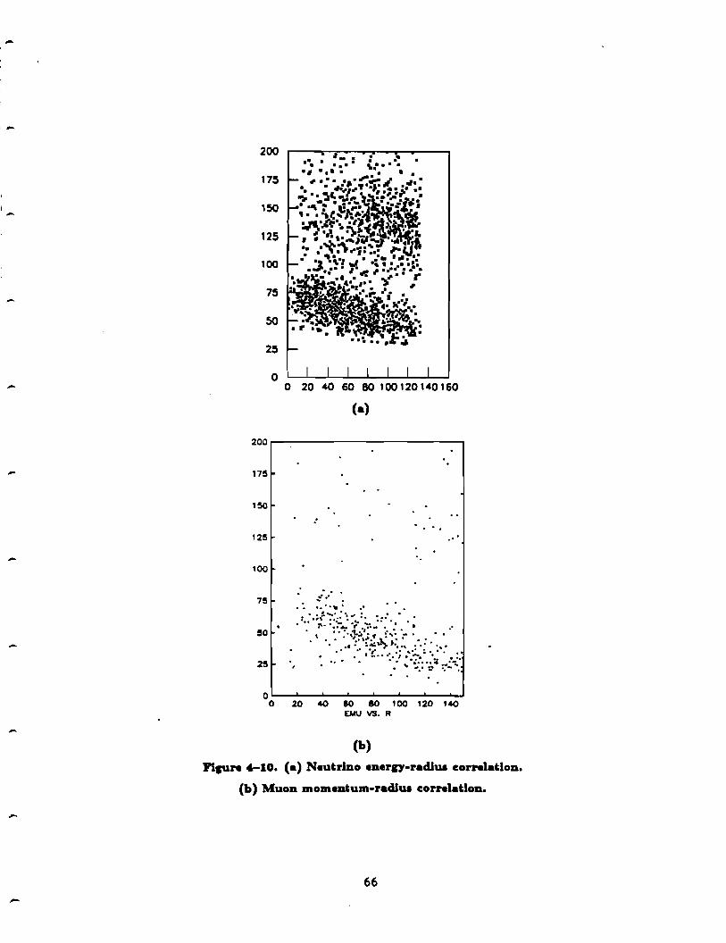
,_
-
-
-
-
-
200
17~
150
125
100
so
2~
0
175
150
125
100
75
50 ...
25 ..
• I • ••• • • :. : -t ••• •• • • • • • • •• • •
# ••••• .,,.~ _,.,. .. . . . ..:,~ "'" .. , ...... : . ..: •• ...... 1,,. -~~~:,.,,:;> • --.,. -- .. - • ~~r-9· ..... :' • :·;. ··.: .. !• h • ··f.'li'"ft ;\'JS ~·M\ •I) f! .~
, • I :\." 3: :i:.tr. L I •
1" , . ..,,.._5 .... V.~ •• ·""-:\ ..... ~ 'f ,. . . ~-. .. ... . • • ... ,._., 1!( .... -; .' ~~:~ .Ja.:• • I '- '._..-: .• • .• ·• . . *. r
·~ .... ,. . '): , o•UOIP'i".llll'-'!'1
1 ••1.•.r. ..
(•)
:
. . . ::· •' ....... .
: ·.;~--:: •. :·~··. :. ::·.
..
.. "" . .. . . ... . . ,·. :·.:.,-t::':·; !,·. · .. : ... ·
.
. • .. ,,:·'t;:.J.,.>:.:" .:.:. ·•• • :• I 'r:. • •:, •; •',~• '; •,: • • :: .. . . .. ~: ·: .. • :-.:.-... . - . ..
o.__ __ ..._ __ _,_ __ _._ __ _._ __ _._ __ ....... __ __.__, 0 20 40 so 80 100 120 140
EMU VS. R
(b)
Flpn 4-10. (a) Neutrino enern-radhu eorrelatlon.
(b) Muon momentum•racllua eorrelatlon.
66

-
-
-
-
-
-
-
-
-0 .,,
.6.QUA51 0 OSIGNAL .,,
0 7
0 .,, .,, II 0
~,.; .... I ... a: c
1:1 ;;; ... -
"" A A A
.,, D
D .,, 0
0.00 2.DD 'I.DO N
6. DD e.oo ID.
Flsun 4-11
B. .. olutlon In neutrino energy ver•u• eut loeatlon n.
chapter, section SC). The best way to distinguish quasielastic pion-band neu
trino events from kaon-band events was to cut on P1,,,, calling all events which
had Pµ > (E,..(R)) + nD",..(R) kaon-band events, where (E,..(R)) was the mean
pion-band energy at the given radius, D'.,(R) was the one standard deviation
spread in the pion-band energy around this, and n = 6. The value of n
was chosen to minimize the error in energy for quasielastic scattering events
(flgure 4-11). This did produce a bias by misidentifying high-11 kaon-band
events as pion-band events and low-u pion-band events in the high-energy
tail as kaon-band events, but this eff'ect was small, and was corrected for by
analyzing Monte Carlo generated events.
67
-
-
-
-
-
-
CHAPTER V. RESULTS
In this chapter we shall describe the two ways in which the data have
been analyzed to search for inverse muon decay. The first section will intro
duce the preliminary cuts applied to the data to isolate the candidate inverse
muon decay events from the background. A description of the active volume
of the detector and an itemization of the number of targets left after cuts
will be given in this section. These cuts were applied to the data before per
forming the two tests, the integrated cross section test and the differential
cross section test, which are described in the two sections that follow. Cross
checks of the results using Monte Carlo generated data are discussed within
each of these sections. The last section of the chapter will give the limits
placed by the present experiment on the parameters of the two non-V -A
theories given in reference 1 and discussed in Chapter 3.
SA. Cuts on the data.
On account of the very large number of triggers taken in the narrow
band beam run (table 4-2) the only practical strategy for searching for a rare
process such as inverse muon decay was by prescreening the data on the basis
of features that may be analyzed by computer. Loose criteria were imposed
to accept all of the quasielastic candidates, while eliminating events that
were clearly irrelevant to the present study-those due to cosmic rays, noise,
inelastic scattering, stray beam muons which intercepted the detector, and
neutral currents. Events that passed these loose cuts were recorded on tape.
68
-
-
-
-
More stringent cuts refined the data sample leaving only fully analyzable
events. These were cuts on the position of the vertex within the fiducial
volume, the proper success codes for the muon tracking package and for the
vertex finding package, the absence of hits around the yertex, and the correct
muon polarity. The events which passed these cuts were called .inverse muon
decay candidates and were analyzed using the techniques to be described in
sections SB and SC.
SA.1. Loose cuts.
To arrive at a set of data of manageable size, the condensed, reformatted
tapes were filtered. There were three conditions applied to the data: ( 1) the
latch for the Quasi trigger (section -iB.3) must have been enabled, (2) the
vertex for the event must have been located successfully using the vertex
package (section 4C.l), and (3) the number of hits in a region about the
vertex must not have exceeded sixty in all three views combined. The first
criterion rejected all events which did not leave hits in the toroid spectrometer
and those which deposited too much energy in the calorimeter proportional
chambers. The second condition eliminated most of the triggers due to ran
dom coincidences and many of the ones that did not originate within the
8.ducial volume. The third criterion (called a "Pacman cu.t" in reference to
the shape of the region around the vertex) rejected events that had a small
shower coming from the vertex which did not deposit enough energy in the
proportional chambers to inhibit the Quasi trigger. An illustration of how
this cut operated is given in figure S-1. The program counted the number
of hits in each of the three flash chamber views which were less than SO cm
from the vertex in that view. (Due to unequal scale factors in the lateral and
longitudinal directions, the contour shown in the figure is an ellipse rather
than a circle.) For each chamber, at most one hit within the boundaries of
69
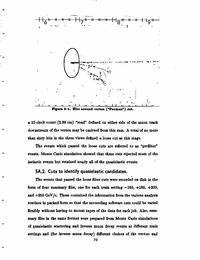
-
-
11 6 11 II II II 11 7 11 II II II 118
11 II II 119
11
- I
.. . -- - f
·-~---- --::· -.... .._: __ .. _...., ---• ..... • .-r
..... • .. ·=·-.-. ---,__ -- -.... . - ...... _;:::, !9 -= - -. -:-..... . : : - -: -:;..t • .... ----- ~:-
- ..... .. .. II II II II I I II " II II I I " II II "
Flsun 1-1. mte around vertex ( •Pacman•) cut.
a 10 clock count (2.39 cm) "road" defined on either side of the muon track
downstream of the vertex may be omitted from this sum. A total of no more
than sixty hits in the three views defined a loose cut at this stage.
The events which passed the loose cuts are referred to as "prefllter"
events. Monte Carlo simulation showed that these cuts rejected most of the
inelastic events but retained nearly all of the quasielastic events.
5A.2. Cuts to identify quasielastic candidates. .
The events that passed the loose filter cuts were recorded on disk in the
form of four summary flies, one for each train setting -165, +165, +200,
and +250 GeV /c. These contained the information from the various analysis
routines in packed form so that the succeeding so~ware cuts could be varied
8.exibly without having to mount tapes of the data for each job. Also, sum
mary tlles ln the same format were prepared from Monte Carlo simulations
of quasielastic scattering and inverse muon decay events at different train
settings and (for inverse muon decay) different choices of the vector- and
70

-
-
axial-vector coupling constants. The true values of kinematic and geometri
cal quantities for these events were available for later comparison with the
measured quantities.
5A.2a. The standard cuts.
The standard cuts applied to the data were the following:
( 1) a vertex must have been found successfully,
(2) the vertex must have been located within the fiducial volume (see
section 5A.2b),
(3) an event must have at least four toroid chamber hits,
(4) in a road around the muon track in the calorimeter, there must have
been an average of at least 0.4 hits per chamber,
(5) a Pacman cut allowing no more than 30 hits in the vicinity of the
vertex was required,
(6) an additional cut on hits downstream of the vertex was applied,
(the "QBOX" cut, described in section 5A.2c),
(7) the muon package must have successfully analyzed the muon tra
jectory,
(8) the muon must have been negatively charged for positive train set
tings, and positively charged for the negative train setting,
(9) the fractional uncertainty in the muon momentum trp/P as deter
mined by the muon tracking package must have been less than 30%,
(10) the goodness-of-6.t quantity x2 /d./. returned by the muon tracking
package must have been less than 16,
( 11) the muon momentum must have been between 10 and 400 Ge V / c,
(12) the maximum slow-out among channels with the hit bit set in any
of the four proportional chambers immediately downstream of the
vertex must have been less than 5.0 V (PTHB:MX cut).
71
-
(13) the sum of slow-outs for channels which had their hit bits set in all
proportional chambers must have been less than 2.0 V (PTHBSM cut).
These cuts are described in more detail in the following subsections.
5A.2b. The fiducial volume.
The portion of the detector within which inverse muon decay candidate
event vertices were accepted was called the fiducial volume. Both the proper
estimation of the number of targets and the measurement of detector and
software acceptances within this volume were important in calculating the
cross section from the data. It was necessary to discriminate against events
that could have been subject to poor analysis by other routines. First of all,
muons originating upstream of the detector were rejected by excluding the
part of the calorimeter upstream of chamber 10. Second, because the vertex
finding package itself performed poorly at large radii where the absorber
material ended, the fiducial volume was defined so as to include only those
events which originated within 150 cm of the center of the neutrino beam.
Finally, because the Pacman cut, the QBOX energy deposition cut (which is
described in the next subsection), and the muon tracking package all assumed
that the event had occurred sufficiently far upstream in the calorimeter to
have left a clear track in the last 50 chambers, the part. of the calorimeter
downstream of chamber 500 was eliminated from the fiducial volume.
The number of target electrons within the fiducial volume was computed
from the known masses and composition of the individual detector elements.
The composition of the detector was important because atoms of different
atomic mass may have different numbers of electrons per unit mass, depend
ing on the ratio of neutrons to protons. Most of the mass in the 6.ducial vol
ume was in the iron and sand absorber planes, but the acrylic in the absorber
extrusions, the oil in the liquid scintillator tanks, and the polypropylene in
72
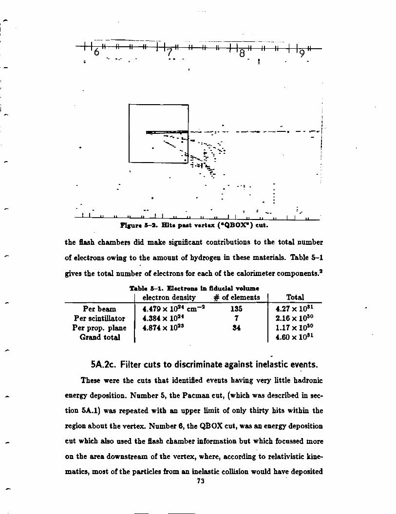
-
-
I 16 II II II II
. --;
II II 11 11 8 11 11 11
- ! I 19 II
I I I
llSl=:::a;;l:oiillllf -..-- --:. : • - -... __ . ._ __ .....,.. ----· - - ..... tr,. - j
I ·,.., • -= -:-_._ ---- -- .. .. .. .....
- ;. - !' -= • -. -:-.._.: = ...._ _____ _,-: -:;.t· ....
~
-- ~::- .
=
--II II II II I I II II II " I I II " II II
Plgure 1-i. mt. put vertu: (•QBOX") cut.
the flash chambers did make significant contributions to the total number
of electrons owing to the amount of hydrogen in these materials. Table 5-1
gives the total number of electrons for each of the calorimeter components.2
Per beam Per scintillator Per prop. plane
Grand total
Table 1-1. Electrom ID fidudal volume electron density # of elements
•.•79 x la2• cm-2 135 •.ss• x lou 1 •. 87' x 1025 3•
Total
•.27x1051
2.16 x 10S0
1.17 x 1050
•.60x1051
SA.2c. Filter cuts to discriminate against inelastic events.
These were the cuts that identified events having very little badronic
energy deposition. Number 5, the Pacman cut, (which was described in sec
tion SA.l) was repeated with an upper limit of only thirty bits within the
region about the vertex. Number 6, the QBOX cut, was an energy deposition
cut which also used the fl.ash chamber information but which focussed more
on the area downstream of the vertex, where, according to relativistic kine
matics, most of the particles from an inelastic collision would have deposited 73 .

-
energy. This cut counted the number of hits in a box about the vertex ex
tending 50 cm upstream to 150 cm downstream and 50 cm on either side.
Hits about the muon track were exempted from the sum, as in the Pacman
cut. (See figure 5-2.) A total of 150 hits in all views was allowed. This cut
was better than the Pacman cut in identifying events where a small number
of hadrons penetrated for some distance before interacting. The cuts on pro
portional tube response, numbers 12 and 13, were included to help identify
events that had energy deposited in an extremely forward direction, where
saturation of the flash chamber response might have limited the usefulness
of the other two filter cuts. The PTHBSM cut (number 13) specialized in
rejecting showers which had penetrated far beyond the event vertex and or
dinary showers with an erroneous event vertex. These cuts were performed
after the others so as to deal with the least number of events, because the
proportional tube information had not been incorporated into the summary
files and had to be read directly off of the event records.
The limits on the Pacman and QBOX cut totals were set approximately
by looking at the noise hit rate in the calorimeter for muon calibration events
scaled by the area of the cut regions. The proportional tube response cuts
were also based on the response of the detector to muon calibration events
(excluding the first few bays which received a high counting rate during the
calibration run) and were relatively loose cuts.
5A.2d. Quality cuts.
The reason for all of the remaining cuts to identify quasielastic candi
dates was simply to ensure that the kinematic and geometric measurements
were of sufficiently high quality to justify further analysis of the event. Most
of them were additional checks on the muon tracking package information,
upon which nearly all of the observed kinematic quantities relied.
74
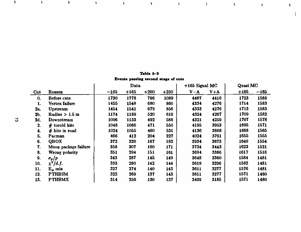
) ) ) )
Table a-i Event. pu•lng Heond •tiage of eub
Data + 165 Signal MC Quasi MC Cut Reason -165 +165 +200 +250 V-A V+A +165 -165
o. Before cuts 1730 1778 796 1089 4461 4416 1723 1588 1. Vertex failure 1455 1548 680 860 4334 4276 1714 1583
2a. Upstream 1454 1541 679 856 4333 4276 1713 1583 2b. Radius > 1.5 m 1174 1189 520 619 4324 4267 1709 1582
-..J 2d. Downstream 1006 1133 492 586 4321 4259 1707 1578 \JI
3. # toroid hits 1048 1086 471 550 4195 3953 1695 1571 4. # hits in road 1024 1055 460 531 4136 3868 1688 1565 5. Pacman 466 412 204 227 4024 3761 1655 1555 6. QBOX 372 320 167 183 3934 3673 1649 1554 7. Muon package failure 358 307 160 171 3734 3443. 1623 1521 8. Wrong polarity 351 294 151 161 3694 3386 1617 1516 9. u,,/p 343 287 145 149 3648 3360 1584 1481
10. x2 /d./. 333 280 142 144 3619 3296 1582 1481 11. Eµ min 327 274 140 143 3611 3277 1576 1481 12. PTHBSM 322 269 137 143 3611 3277 1571 1480 13. PTHBMX 314 259 130 137 3499 3185 1571 1480
-
SA.2e. Rejection rates.
Table 5-2 summarizes the number of events left after each cut for the
data and for Monte Carlo events. The Monte Carlo events were generated in a
volume larger than the actual fiducial volume to simulate the contamination
due to events which were generated outside of the fiducial volume. Only
those events which had been generated within the fiducial volume have been
counted in this table. Figure 5-3 displays the fraction of events that survived
each cut for each data sample with cut numbers from section 5A.2a along
the horizontal axes and percent rejected plotted vertically. The rejection
of each of the first six cuts, which discriminate against inelastic events, is
shown in the first plot for the data alone. The events which were ultimately
rejected because of failures in vertex finding (number 1) had been included
on the original condensed data tapes because they had been accepted by
older version of the package. These were, in most cases, beyond the edges
of the fiducial volume. The next major cut was the one that rejected events
with vertices outside the fiducial volume (number 2). One can see the large
number of events rejected by the second stage Pacman cut (cut number 5)
and by the QBOX cut (number 6) due to hadronic energy deposition. The
remaining plots show how the remaining cuts aft'ected the data and the two
Monte Carlo simulations, giving similar rejection rates. All .of these cuts were
below the 10% level. From the plots for signal and background Monte Carlo
events one may note the rather low level of rejections overall. There was a
higher rate of rejection by the muon tracking package (number 7) for the
inverse muon decay events because of the large number of tracks that passed
through the holes in the toroids. The increase in the momentum uncertainty
(number 9) at the higher train settings for quasielastic scattering events may
reflect the increasing muon angle, which decreased the path length in the
76
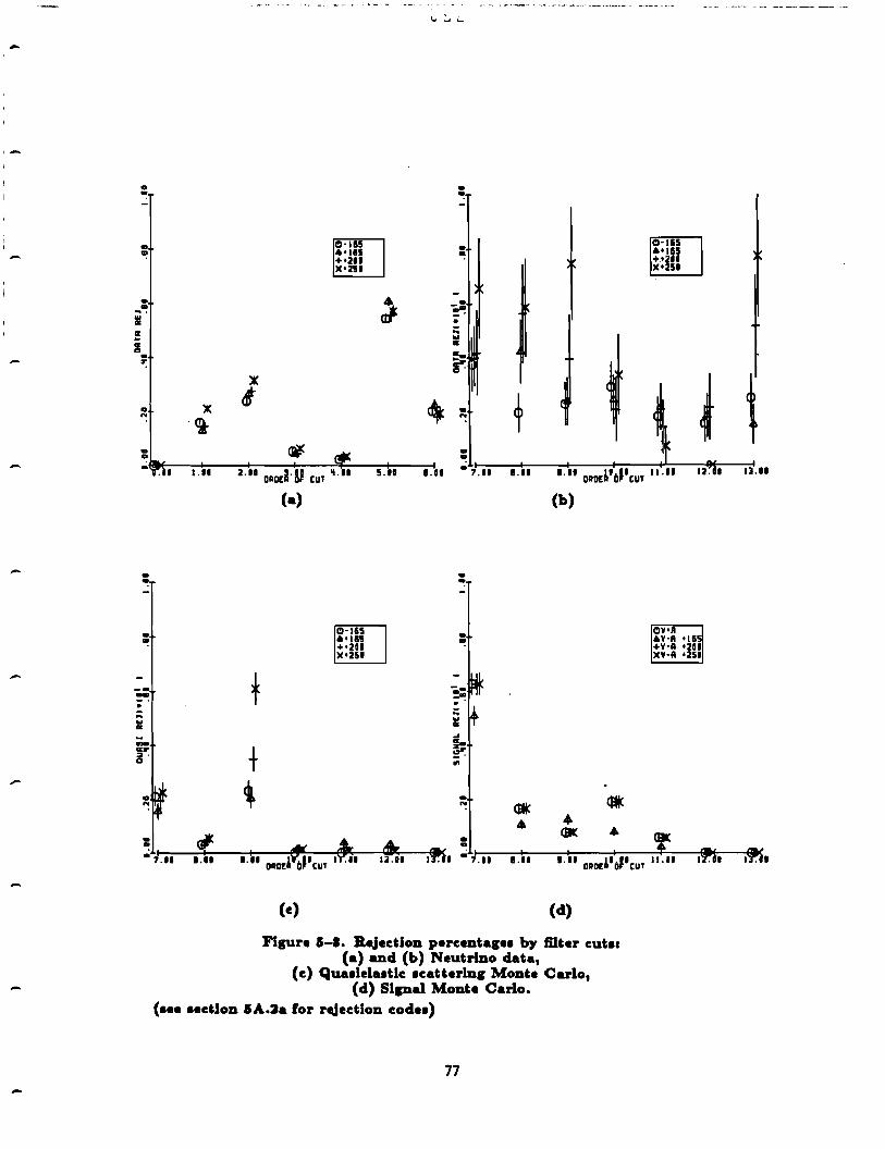
• "'!
• "!
. • ... ... • er
i . "'.
0 N
• • -
• -• ..
---.. ... • ... a::r ::I. a
x ~
. I I.II
• "'!
0·165 • 0·165 ••115 "! ••IH +•211 +•211 )(•251 )(•251
~ -= -· . :: "' Ill
~ I":
x I
~ ~ • ~
'*' • "'! 2. II 011oel 8J CUT •t. II 5.11 .... • 7.11 . ... .... DllOE~·oJ'cuT II.II
(a)
(e)
0·165 ••165 +•211 )(•251
• -• ..
:;
= ~ ·-3:r -. ..
(b)
(d)
Figure 1-1. Rejedlon percentagH by filter cubs (a) and {b) Neutrino data,
(e) Qua1lela1tle 1catterlng Monte Carlo, {d) Slsnal Monte Carlo.
(1ee Hdlon IA.2a for rejection eodH)
77
' t 12. ' 13.11

------ - ··~----------·~--····-·-----· _.-... ·----~--
toroid magnets.
So, within the limits of statistical and systematic error, the data and
Monte Carlo sets of events seemed to behave reasonably under the cuts which
were imposed. For the earlier filter cuts (numbers 1 to 6) comparison with
Monte Carlo would make no sense (because the inelastic portion of the sam
ple was not modelled) and the only cross-Check was to compare the positive
train settings to the negative setting. Since the Pacman and QBOX cuts
had roughly the same rate of rejections, we might assume that these did not
significantly reject isolated recoil protons (which were present for the neu
trino quasielastic events). The polarity cut (number 8) and the proportional
chamber cuts (numbers 12 and 13) exhibited the main discrepancies between
data a.nd Monte Carlo sets among the latter seven cuts. These were again
readily understood in terms of contamination of the data sample.
58. The integrated cross section tests.
58.1. The Q2 distributions.
With the candidate inverse muon decay samples, we could attempt to
do the same sort of analysis that had been done using wide band neutrino
beams to identify a l6w-Q2 excess in the neutrino events as compared to the
antineutrino events. Q' was reconstructed from the measu:ced quantities by
the formula:
(5.1)
The exact expression for this quantity was Q1 = -m! + 2E"(E" -p" cos8")
but this formula had the undesirable property of giving negative values when
applied to events from kaon-band neutrinos which bad been misidentified
as pion-band neutrinos. This would have made the computation of nuclear
corrections for the quasielastic scattering events impossible, so the slight Q1
78

-
;
:s 17.5 L
14 ~5.
12 1Z.5
10
8
6
4
-" 2 "-·-
c Cl. 0. 05 1. 1.5 2. 0. 0.5 1. 1.5 2.
0-SO FOR (-) FINAL a-so FOR 165
(•) (b)
..
9 I 10
8
7 8
6
6 r --,
~ " 4
3
2 2
O'---'-.......__._~..___._~...Jll...~..i...L..l.Llo:..i..;__J 0'---'-~-'-~'----1.1..u....i...J1.....1..__.__..L...11......:.u..u
o. 05 1. 1.5 2. 0. 0.5 1. 1.5 2. FINA~ o-sa FO!" ... :~ .. : FINAL 0-50 FOR +2~0
(c) (d)
Figure 1-4. Q2 dlatrlbutlo:m, (a) -185, (b) +ies, (c) +ioo, (d) +350 GeV /c.
79
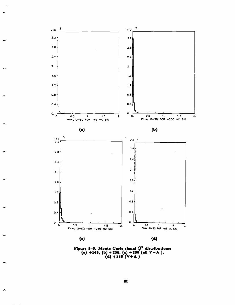
-
-
-
•10 3
3.2 3.2
2.8 2.8
2.4 2.4
2. 2.
1.6 i .6
1.2 1 .2
o.e 0.8
0.4 l 0.
0.4
l 0.
0. 0.5 1. 1.5 2. 0. 0.5 1. 1.5 F'l~!AL 0-50 F'OR 16~ "4C S:G F':r·!"'L 0-SQ F'OR +200 i.tC S•G
(•) (b)
·1 ·'J 3 ~ :u ~---------------.. .~o
2.B
2.4
2.
1 6
1.2
0.8
c.
I I
2.6 ~ j• .I
ii :i 2.4 n
ii :1 I•
2. ~
11 I.Sn
,,~ o.e 1
0.4
0. i...:i.-..__......._......__ .......... _..._........__...__J 0.5 1. 1 .5 2. 0. 0.5 1. 1.5
F'ltlAl. 0-SQ F'OR +250 MC SIG Fll\IAL o-sc roR , 65 t.IC SIC
(c) (d)
Figure 1-1. Monte Carlo •lgnal Q2 dl•ti-lbutloDS1 (•) +181, (b) +ioo, (c) +iso (all V-A ),
(d) +181 (V+A)
80
2.
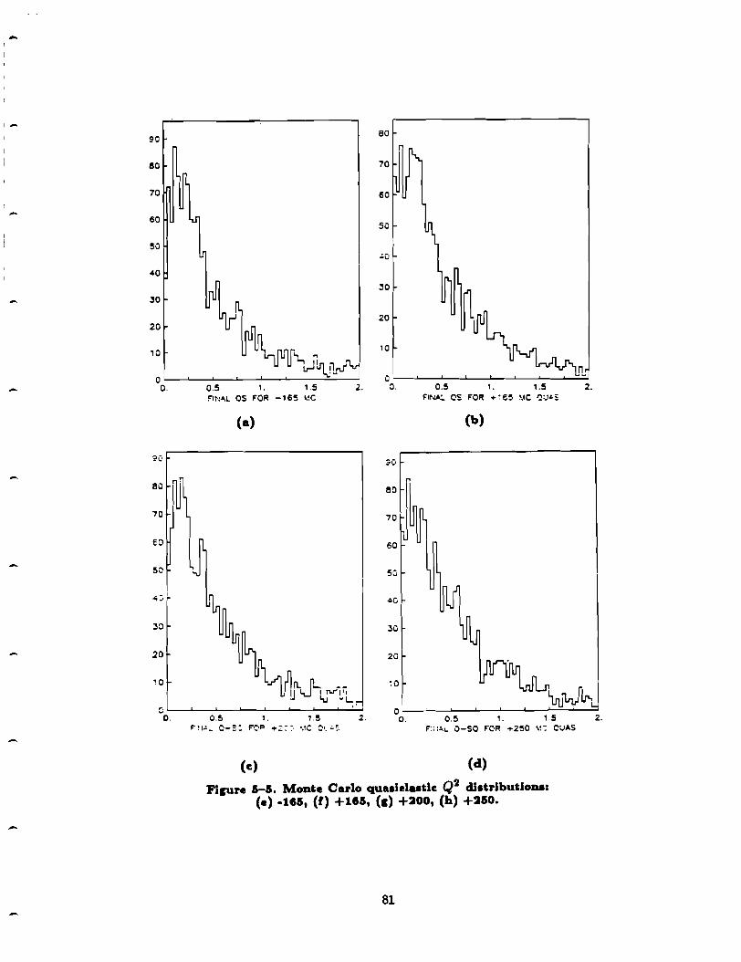
-
,_ !?O
ea
70
60
so
40
30
20
10
0 a.
~C·
80
ru 70
eo
so
4~
30
20
io
c o.
60
70
60
50
.. a L
30
~1J\.J\J1,.t 20
10
0 0.5 1. 1.5 2.. 0. 0.5 1. 1.5 2. !"1~:.•.L OS FOR - 1 65 MC FINA:.. OS FOR +~€5 MC ~:Jt.S
(a) (b)
3C•
ri
60
70
60
50
40
30
20
,n.J.... -- ~o LI i ;v,,,
Lu v L..
0 o.s 1. 1.5 .... o. 0.5 1 . 1.5
~!1:._ Q-S:·: f"0P +::':· •.1c o•_·.;.::_ F":; ;.:..L 0-SO F'OR +250 \~: CUAS
(c:) {d)
Figure 5-5. Monte Carlo qua•lela•tlc: Q2 dl•trlbutlonas (•)-tea, {f) +iea, (s) +ioo, {h) +iao.
81
2.

-
,_ error in equation 5.1 for the inverse muon decay events was tolerated. On ac
count of the extremely small muon angles, a systematic correction for beam
divergence, amounting to nearly 1 mrad at a radius of 150 cm, has been
applied. The distributions in Q2 (measured in GeV2 ) for the various train
settings are shown in figure S-4. For comparison, the distributions obtained
from analysis of the Monte Carlo simulations of pure quasielastic scattering
events and of pure inverse muon decay signal are given in figure S-5. These
show the slight broadening of the Q2 distribution for signal with increasing
average neutrino energy, as well as the independence of the distribution for
the quasielastic background. Because the shape of the background was in
sensitive to the energy of the neutrino, it was possible to perform a straight
subtraction between the distributions for different train settings. The orig
inal bin width was chosen to be comparable to the instrumental resolution;
in fact, the true Q2 distribution for the inverse muon decay Monte Carlo
sample was contained primarily within the first bin (Figure 5-5 a through
d). Events with Q2 > 2.0 GeV2 were ignored to reduce the contamination of
the small number of inelastic scattering events in the distributions.
In order to compare the various distributions so as to check for a low-Q2
excess we grouped the original binned data into bins containing approxi
mately equal numbers of Monte Carlo quasielastic scattering events. Fig
ure 5-6 plots the low edge in Q2 for each of the bins at the various train
settings. The number of bins was chosen to optimize the resolution in Q2
while minimizing the sensitivity to statistical fluctuations3 by requiring that
no more than 20% of the new bins contain fewer than five quasielastic can
didate events for the data. The rest of the Q2 .study used the rebinned data
only.
Since the nuclei of the target material were not precisely isoscalar, the
82

-
I,_
I
I.II
1.4
.,..... 1.2
1.
0.2
1.4
1.2
I.
o.e
0.6
o . .a
0.2
-
-
I.Ii
1.4
1.2
I.
o.e
0.1
0.4
0.2
4 I 12 ,, 20 ~·
£1 02 RCB-NG
2 4 I I 10 12 14 11 02 R[81,...ING
(a) (b)
2 4 I I 10 12 ,.. ,, 02 REB-lt«i
(e)
Figure 5-8. Reblnnlng •cheme In Q2 (bin number v1. low edge). (a) +185, (b) +300, (e) +350
83
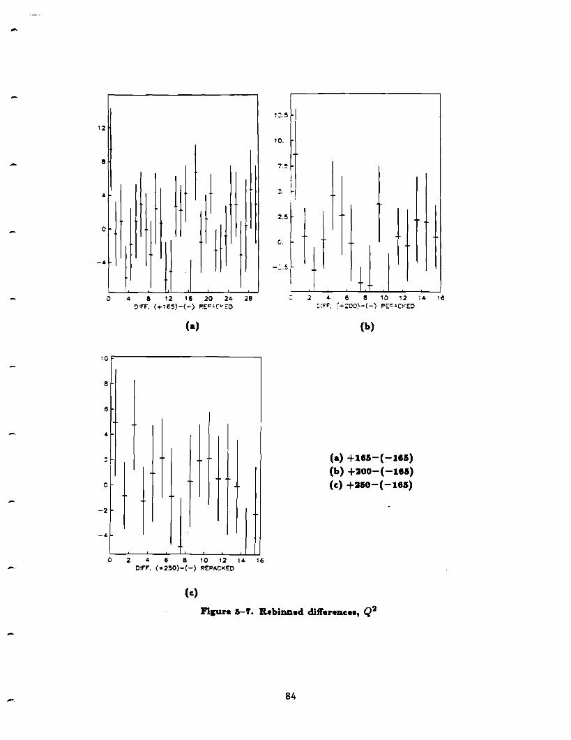
-
-·
12
II
j l I 4
0 I . -4
0 4 8 , 2 , 6 20 24 28 !:>'FT. (+1es)-{-) P.E~"C"'E:O
(a)
8
6
4
.. , .
c
-2
0 2 4 6 8 10 12 14 16 O!F"F", (+250)-(-) REF'ACKEO
(e)
i:.5
10.
7.~
=
2.5
Ci .
-.:..:
I
I l I
I ... ,
r I 1 i- j r ~ ff I t ., 2 4 6 II 10 12 a 16
:.-:""F". {+ZOO)-{-) p:;c~C!".ED
(b)
(a) +115-(-115) (b) +ioo-(-115) (e) +i5o-(-115)
Figure 5-f. Re binned dlff'ereneee, Q2
84

-
-
nuclear effects (Pauli suppression) at low Q2 gave different values for
neutrino-induced quasielastic scattering events and for antineutrino-ind11ced
events (section 3C) in the Q2 region of interest. We used equation (2.5)
to Bnd the nuclear correction for each, after determining the average value
of 141 at the center of each Q2 bin using equation (2.6). The antineutrino
distribution was then multiplied by the ratio of correction factors.
We normalized the rebinned antineutrino distribution to the neutrino
distribution to have the same area past the Brst bin, before subtracting it.
This yielded the series of difference plots shown in Bgure 5-7. In each of
these plots, the abscissa is the rebinned Q2 given in figure 5-6. An excess
of events in the lowest Q2 bin was interpreted as being a signal for inverse
muon decay. The error bar for each bin was calculated on the basis of the bin
contents of the histograms being subtracted, using Poisson statistics, before
normalization. These statistical errors dominated over the systematic errors
from the nuclear correction process.
Table 1-1. ObHrved and expeded low-Q2 exce11ea. V-A V+A
Train setting Observed Expected Expected
+165 9.5± •. 9 7.2 2.•
+200 s.6±•.5 •. o l.• +250 4.9± •. 2 5.6 1.9
All positives 23.0±7.9 16.9 5.7
Likelihood ratio V-A vs. V+A: 7.0
Table 5-3 gives the Q2 inverse muon decay signal for each train setting.
In this table, also, are the numbers of events as predicted by the pure V-A
and pure V+A models, which were calculated in the following manner:
I {''"'··<•> "" (ur) = die/>(•) Jo d11 du(•) (5.2)
85
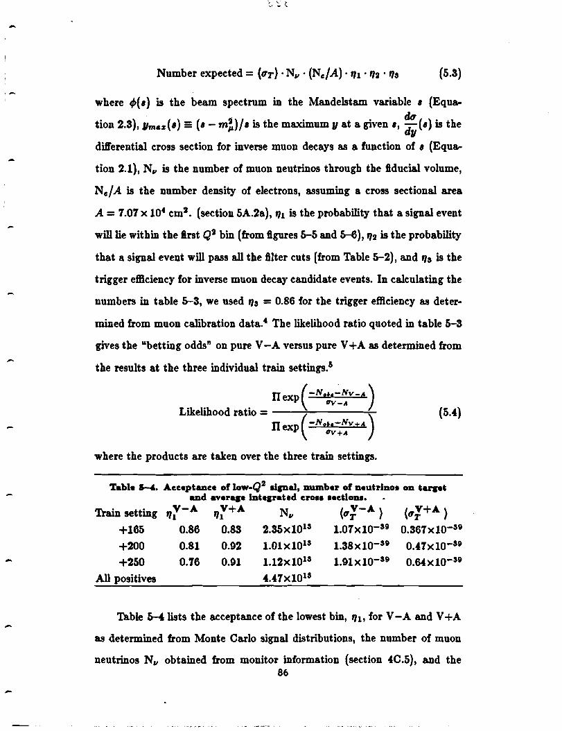
-
,_ I
-
-
-
-
Number expected= (D'T) • Nv ·(Ne/A)· '11 • '12 ·'la (5.3)
where </>( 1) is the beam spectrum in the Mandelstam variable 1 (Equa
tion 2.3), Jlmu(•) = (1 - m!)/1 is the maximum 1J at a given 1, : (1) is the
diff'erential cross section for inverse muon decays as a function of 1 (Equa
tion 2.1), Nv is the number of muon neutrinos through the fiducial volume,
Ne/A is the number density of electrons, assuming a cross sectional area
A = 7.07 x 104 cm2 • (section 5A.2a), q1 is the probability that a signal event
will lie within the lrst Q2 bin (from figures 5-5 and 5-6), '12 is the probability
that a signal event will pass all the filter cuts (from Table 5-2), and 'la is the
trigger efficiency for inverse muon decay candidate events. In calculating the
numbers in table 5-3, we used 'la = 0.86 for the trigger efficiency as deter
mined from muon calibration data.4 The likelihood ratio quoted in table 5-3
gives the "betting odds" on pure V -A versus pure V +A as determined from
the results at the three individual train settings. 5
Ilexp(-N,..-Nv-A)
Likelihood ratio = ( ""-• ) Ilexp -Neta-Nv+A
O'V+A
where the products are taken over the three train settings.
(5.4)
Table 1-4.. .Acceptance of Iow-Q2 •lgnal, number of neutrino• on target and averqe Jnte1rated CrDH Hdlom.
Train setting ,,"'[-A. q"'f +A. N,, (0'9{-A. ) (O'~+A. )
0.367x10-a9 +165 0.86 0.83 2.35xl013 1.01x10-a9
+200
+250
All positives
0.81
0.76
0.92
0.91
1.01x10¹³
1.12xl013
4.47x10¹³
l.38x10-39 0.47x10-39
1.9lxl0-a9 0.64x10-a9
Table H lists the acceptance of the lowest bin, q1 , for V-A and V +A
as determined from Monte Carlo signal distributions, the number of muon
neutrinos N,, obtained from monitor information (section 4C.5), and the 86
-1-
1
average integrated cross section (D'T} in units of cm2 for V-A and V +A , at
each train setting.
SB.2. The E62 distributions.
An analogous analysis of the distributions in E µB: was carried out, and
is illustrated by figures S-8 to S-11. Here, as before, the muon angle has
been corrected for beam divergence, and the data were rebinned on the basis
of Monte Carlo distributions, with a maximum EB2 of 40 MeV. The signal
distributions were nearly identical for the diB'erent train settings, because of •
the relationship
EB2 = 2me(l - g) (5.5)
and the slow dependence of llmu on E11 • In this variable the shape of the
background changed with beam energy and an expression for the nuclear was
not available, so it was not possible to normalize the data for diB'erent train
settings simply. Therefore, the antineutrino data were simply multiplied by
the bin by bin ratio of the Monte Carlo quasielastic scattering distributions
for the appropriate positive train setting and for the -165 GeV antineu
trino setting. This correction was carried out on the basis of the Monte
Carlo quasielastic scattering distributions in figure S-9. The neutrino and
antineutrino data were normalized to have equal totals from the second bin
to 40 Me V before subtraction.
The results of the rebinned diB'erences are given in table S-5 along with
the number of expected excesses in the 0 < EB2 < 1.5 MeV bin. Because
of the theoretical constancy of the EB2 distributions, the calculation of the
expected number of events diB'ered from that done in the Q2 analysis by
replacing the r11 factors with a single acceptance factor, "' = 0.86, for all
train settings. Due to the uncertainty in the nuclear correction and because
of the diftlculty of estimating the covariance of these results with those from
87
----~ - -----·------~- .. n---,..--·-.~-·~---~-·----... -.•-.-...,...--_-···_·-------------------

....
14
1-i 16
12 14
10 12
B 10
8 6
6
4
2 2
O'----..:.~-'-~-L-~-'-~LL..-~~..u.....i--'
c 4 8 12 16 20 24 28 4 8 12 16 20 24 28 E-TH2 F"OR -1 €~ E-TH2 FOR +165
(•) {b)
10 9
8
8 7
6
6
4
3
2 2
n
0'--..LL....1-"--..IJ .................... .._ ......... __.. .............................................
0 " 8 , 2 , 6 20 24 28
E-TH2 FOq +::-::i
o:------_.___.__w.u_JJ.WL..lli.LL~I! 0 4 12 16 20 24 28
E-TH2 FOR +:~o
(c) {d)
Figure 5-8. E92 dl•tributlom (•) ·115, {b) +115, (c) +:aoo, {d) +350 GeV /c
88

-
,-
-
-
2.4 ~.4
2. 2.
1.6
1.2 1.2
D.11 o.e
0.4 04
L I 12 16 20 24
E-TH2 FDR +115~ MC SIG 21
0. 0 4
, c.
I 12 16 20 24 E-TH2 FOR +200 MC SIG
0 4
(a) (b)
·'.~ 3 ,...-~~~~~~~~~~-
2.4 2. ~
n t.75 H
2.
1.8
ll t.5 ~
t.25 ~
0.8
1. ! 0.75
0.5
0.4 • 0.25
o. 0. 0 4 8 1 2 1 6 20 24 21 o 4 e 12 11 20 24 a
E-TH::? FOR +2~0 MC SIG E-1'>42 roR +165 MC SIG
(e) (d)
Figure 5-9. Monte Carlo algnal E92 dlatrlbutlona: (a) +165, (b) +:aoo, (e) +Ho (all V-A ),
(d) +165 (V+A)
89
21

-
-
70
150
~o
40
20
10
Ql...----'~--'~--'-~--'-~--'-~-'-~--'--'
70
60
so
30
20
10
0 4 8 12 16 20 24 28 E-TH2 FOR -165 MC
(•)
~1~fl~riJl.J O'--~L-----''----'~--'~--'-~--'-~~~--.....J
0 8 12 16 20 24 2!!
(c)
70
60
~o
40
30
20
IC
0'------''------'~---'-~--'-~-'-~---'-~~-'
100
eo
60
40
20
0 4 8 12 1 6 20 24 26 E-TH2 FOR +165 MC QUAS
(b)
C'------'~--'~--'-~--'-~-'-~---'-~--'--'
0 4 8 12 16 20 24 28 E-rH2 FO~ +2~0 W.C OUAS
(d)
Flsure 1-9. Monte Carlo quaai•laatlc E82 dlatrlbutlonsa (•) -111, (f) +111, (s) +~oo, (h) +no.
90
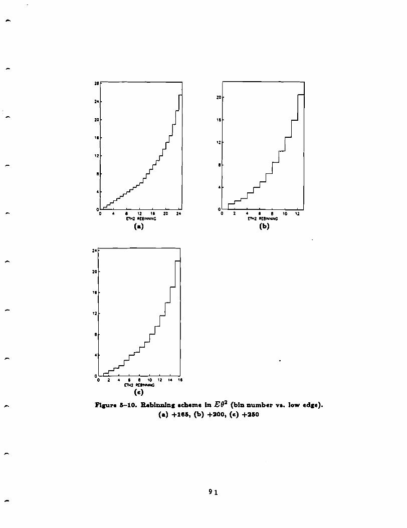
-
-
21
2•
20
18
12
I
"
" I 12 18 20 2• £Tl<2 l!El-"C
(a)
2•
20
18
12
I
2 • I I 10 12 1.a 18 E'TM2 l!EIMlllllC
(e)
20
18
12
I
O..._._._~_,_~....____.~....._~......_.
0 2 • I I 10 12 £Tl<2 1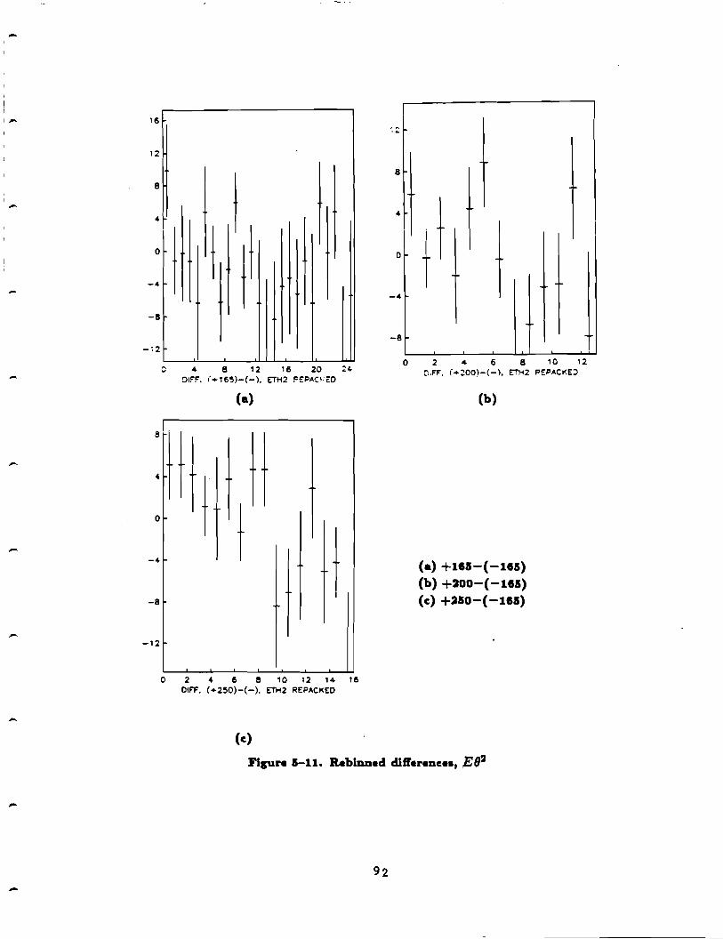
-
,_ 16
12
8
0
-e
-~2
--8
-12
-
'
-c 4 8 12 16 20 ~I.
OJ!"!", (+1155)-(-). ETH:! FEPAC!·C:D
(a)
t I
0 2 4 6 8 10 12 14 16 OIFF', (+250)-(-). ETH2 REPACKED
(c)
0
-8
0 2 4 6 8 10 12 ::;.FF, (+WO)-(-), E"!"!-i2 PEPACKEJ
(b)
(a) +115-(-115) (b) +:aoo-(-115) (c) +350-(-115)
Figure 5-11. Reblnned dlfl'erencH, E92
--- ------------------
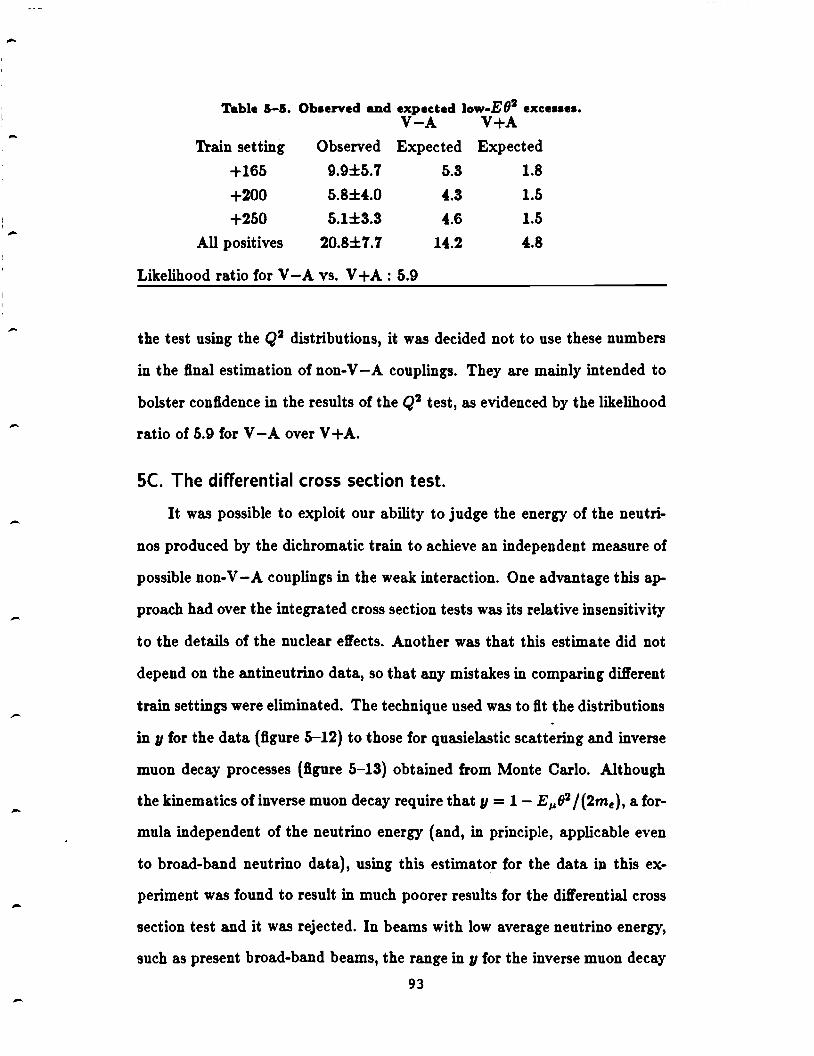
-
-
-
-
-
Table 1-5. ObHrved and expected low-E 92 exceHH. V-A V+A
Train setting Observed Expected Expected
+165 9.9±5.7 5.3 1.8
+200 5.8±4.0 4.3 1.5
+250 5.1±3.3 4.6 1.5
All positives 20.8±7.7 14.2 4.8
Likelihood ratio for V-A vs. V +A : 5.9
the test using the Q2 distributions, it was decided not to use these numbers
in the final estimation of non-V -A couplings. They are mainly intended to
bolster confidence in the results of the Q2 test, as evidenced by the likelihood
ratio of 5.9 for V-A over V +A.
SC. The differential cross section test.
It was possible to exploit our ability to judge the energy of the neutri
nos produced by the dichromatic train to achieve an independent measure of
possible non-V -A couplings in the weak interaction. One advantage this ap
proach had over the integrated cross section tests was its relative insensitivity
to the details of the nuclear effects. Another was that this estimate did not
depend on the antineutrino data, so that any mistakes in comparing different
train settings were eliminated. The technique used was to fit the distributions
in 11 for the data (figure 5-12) to those for quasielastic scattering and inverse
muon decay processes {figure 5-13) obtained from Monte Carlo. Although
the kinematics of inverse muon decay require that 11=1- Eµ82 /(2me), a for
mula independent of the neutrino energy (and, in principle, applicable even
to broad-band neutrino data), using this estimator for the data in this ex
periment was found to result in much poorer results for the differential cross
section test and it was rejected. In beams with low average neutrino energy,
such as present broad-band beams, the range in 11 for the inverse muon decay
93
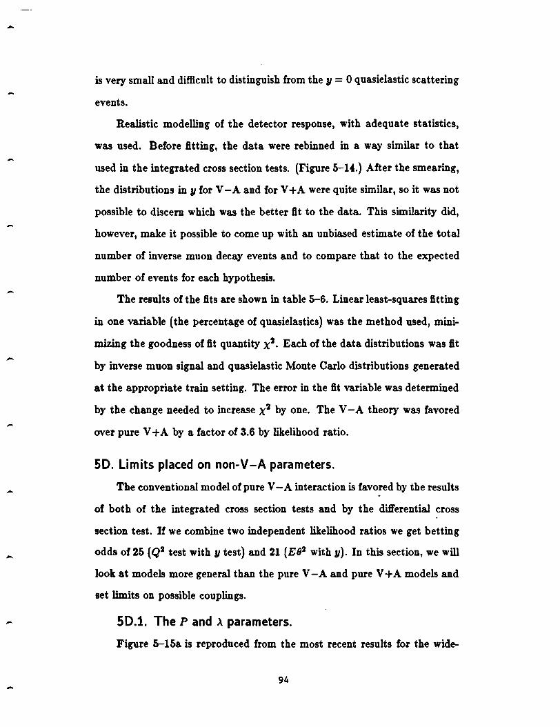
-
-
-
is very small and difficult to distinguish from the 11 = 0 quasielastic scattering
events.
Realistic modelling of the detector response, with adequate statistics,
was used. Before fitting, the data were rebinned in a way similar to that
used in the integrated cross section tests. (Figure S-U.) After the smearing,
the distributions in 11 for V-A and for V+A were quite similar, so it was not
possible to discern which was the better flt to the data. This similarity did,
however, make it possible to come up with an unbiased estimate of the total
number of inverse muon decay events and to compare that to the expected
number of events for each hypothesis.
The results of the fits are shown in table 5-6. Linear least-squares fitting
in one variable (the percentage of qua.sielastics) was the method used, mini
mizing the goodness of fit quantity x2 • Each of the data distributions was fit
by inverse muon signal and quasielastic Monte Carlo distributions generated
at the appropriate train setting. The error in the fit variable was determined
by the change needed to increase x2 by one. The V -A theory was favored
over pure V +A by a factor of 3.6 by likelihood ratio.
50. Limits placed on non-V-A parameters.
The conventional model of pure V -A interaction is favored by the results
of both of the integrated cross section tests and by the difl'erential cross
section test. If we combine two independent likelihood ratios we get betting
odds of 25 (Q2 test with 11 test) and 21 (E82 with 11). In this section, we will
look at models more general than the pure V-A and pure V +A models and
set limits on possible couplings.
50.1. The P and .\ parameters.
Figure 5-15a is reproduced from the most recent results for the wide-
94

..
20. -~.~
17.5 '.5. ~ I
15. •Bf 12.5
~J J - I
10. ~ I
10. i I
7.!~
7.5 . ~ 5.
2.5 2.5
0. -o~ o. 0.5 1. -1. -0.5 o. 0.5 1.
Y MEAS, DATA Y lolEAS, CATA
- (•) (b)
. : i
4
3
2 --o.s o. o.5 1. -1. -0.5 o. 0.5 1.
Y MEAS, DATA Y MEAS, CATA
(c) (d)
Figure s-1i. U dletrlbutloll8 (•) -165, (b) +165, (e) +ioo, (d) +i5o GeV /e
-95
-
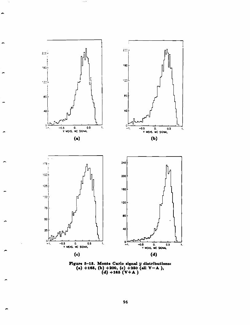
-
-
i:-: ~
f~ i I
i ·s:i ~
I
I I I ,r: '":::.. ~ Lli I ; ) I
"l 40 I I
I ~J.r-- lf'.. _J ' .•
I
~ 7~ -
I
~ s~ r I
:25 l I
I I .. ~o-I
7sl
!IC
25
0 -1.
-o.5 0. 0.5 1.
Y ME!S. MC SIG..,AL Y M~S. MC SIGNAL
(•) (b)
2.&0
200
160
120
110
~~ 0 -0.5 0. 0.5 1. -1. -0.5 o. 0.5
Y UEAS. UC SIGNAL Y MEAS. ltlC SIGNAL
(c) (d)
Figure 1-11. Monte Carlo •lgnal 1J d.i•trlbutlo119: (•) +111, (b) +200, (c) +210 (all V-A ),
(d) +HI (V+A)
96
1.
1.
-
70 •: ~
IO :o i
50 7C f eor
! :io~
,ol r 1i·
J !;i
JO
i ~o i-
20 I I
20
-0.5 o. 0.5 1. -o.:i 0. o.:i , . Y MEAS. UC QUASI$ Y MEAS. I.IC OL;AS:S
(•) (b)
---I
~ I
60 ~ e: r ;
f I i I
~o i 50
I I
40L £0
~ ~ i
~c '~~ 20 ,, 20 -~ 10 10
0 -1. -o.:i 0. o.:i , . 0
-1. -o.:i 0. o.:i , . Y ll[AS, MC OUASIS - Y llEAS. MC OUASIS
(c) (d)
Figure 5-11. Monte Carlo qua1lela.tlc 1J dl.trlbutlona1 (e) -181, (f) +111, (g) +200, (h) +210.
97 -

-
-
-
1.
-0.75
-1. 0 • • 12 11 20 •• 3
·~f 0.5 f 0.25
Q. L
-0.25
-0.5
-1.
• 165 Y llt[ltNNINC
(•)
0 z • • 10 12 14 +2'0 Y 111[91NNlllG
(c)
0.75
0.5
o.
-0.5
-0.75
-1. 0 2 • • • 10 12 14
+ 200 Y llD!INNlllG
(b)
Figure 5-1'· lteblnnlng •chem• In II• (a) +181, (b) +200, (c) +210
98

-
-
Table 5-8. Fltl to 11 dl•tirJbuUom. V-A V+A
Train setting Observed Expected Expected
+165 9.8±8.8 10.0 3.4
+200 15.1±11.6 5.8 2.0
+250 19.9±10.8 8.5 2.8
All positives 43.9±18.1 24.3 8.2
Likelihood ratio for V-A vs. V +A : 3.6
band beam study of the inverse muon decay reaction.6 It depicts the 90%
confidence level limits on P and .\ for the Gargamelle and CHARM detec
tor experiments. Figure 5-15b gives the same plot for this experiment using
the results of the tests described in the preceeding two sections of this thesis.
For each train setting, the ratio S = N0 b1 /NYz;A was formed. The measure
ments of S from the Q2 test are independent for different train settings up
to the common dependence on the -165 data distribution and on the -165
Monte Carlo qua.sielastic distribution for the nuclear corrections. Also, this
test and the 11 distribution test did rely on a common set of assumptions that
went into the formulation of the Monte Carlo simulations for inverse muon
decays and for quasielastic scattering events. The errors on S were com
puted by combining the statistical errors with those imposed by limitations
in estimating the total number of neutrinos (5% error in _normalization),7
the fiducial mass (3% error in the number of electrons),8 and the various
acceptances denoted by r11, q2, q3 above (binomial error). When the errors
were added in quadrature, the statistical errors clearly dominated.
When we combined the different measurements of S, treating them as
independent measurements, we found S = 1.00 ± 0.28 for the best fit and ltr
limit. Due to the rather small sample of inverse muon decay events in this
experiment ( ~ 20 versus 600 for the ·CHARM experiment) the limits were
much less restrictive. To the level of accuracy attainable by this technique, 99
. ------------------

-
-
-
-
-; .. I-;. ]f 'i I • 01------+------."""'4., 90"4c.L,, ... ~ .... . ~ ---z z GGM,•
• a
-
I
/ , ....... I IHO
I I
I I
0
>.· -2!y" •tl·••l (a)
··..----------r-------..........
-"' -··+---------+-------~ --Ill --'-1. aa - .so I. aaLA"BOA . 50 I. DO
(b)
thl1 expt.
"f"Orld average
Flsun 1-11. 90% confidence limit• on non• V-A parameter• P and .\1 (a) for Gargamelle and CHARM, (Ref. I) (b) for thi1 experiment
100

-
-
-
-
-
however, it is clear that our results are in agreement with previous ones
and with the pure V-A theory as well. The dotted contour in figure 5-15b
shows the result obtained by combining the value for S from the CHARM
experiment (S = 0.98 ± 0.12) with the value from this experiment:
s = 0.982 ± 0.110 (5.6)
Both of these contours were obtained from the one-sided 90% confidence
interval for the normal distribution: (-1.966 < S - {S) < oo ). This will tend
to underestimate the errors on P and on.\ if {S) is greater than one, but we
have chosen this method in order to be consistent with previous plots of the
limits on these parameters.
50.2. Limits on the general V. A parameters.
Table 5-7a sets out the limits imposed on the angular parameters for the
fermion-mirror fermion mixing models of Maalampi et al.1 by a least squares
flt to the most recent results to the various tests described in Chapter 3.
The dependence on the cross section of inverse muon decay is described in
Appendix B. The value of S used was the world average (equation 5.6). The
new values of S and u(S) left the values of the parameters of these models
virtually unchanged (compare to table 3-2a). The contributions to x2 by the .
experimental constraints used are listed by size (for model "c") in table 5-8
to indicate how the fits were more in8uenced by constraints other than the
inverse muon decay cross section.
Table 5-7b gives the results for the left-right symmetric model in the
same format as table 3-2b. Here the revised value for S had no effect on the
best flt for the model parameters or on the errors. Figure 5-16 shows the
68.5% confidence limit region (outer contours) and best flt (inner) contours
in parameter space, using the old value of S, the value obtained by this 101

)
... 0 N
) )
Model fJ, 8emu
&coh 1.1 2.lt
&me free* free heoh 1.1 1.9 hine free free c 5.0 13.3 dcoh 0.1 43.6t dine free free
Table I-fa B.e•ulti• to &ti• for fermion-mirror fernalon modela
(world nerage Yal1U1 for S) Be•ti ftti• -d 11.1" C.L. Yalue•
"'' t/>emu ,,,..
(JIAma.11 ti>,. 8.0 15.7 0.0 2.3 8.9 5.5 15.0 free free 7.6
16.0 25.0 0.0 3.8 0.0 15.9 24.9 free free 0.0 14.0 18.8 2.5 9.2 13.9 4.4 7.1 0.0 1.6 9.0 4.3 7.0 free free 7.8
•uncomtiralnecl parameter tParabollc error fttilmatie
All Yalu .. In d•sn••· Pun V-A. stv•• .. ro for .U mixing anglH.
Table 1-fb B.e•ulh to &ti for the left-right; •ymmetirlc model
(world average Yalue for S)
Quantity Fit value
0.14 0.0°
68.3% C.L.
0.18 1.90
x2 = 3.0 for 5 degrees of freedom. Pun V-A. vi11U1 I• uro for eam parameter.
tl>Pmu sin2 6w
- 13.6 0.249 12.1 0.2-16 44.9t 0.240
4.7 0.2t0 18.2 0.221 13.7 0.2·i9 12.1 0.246
x2 /d.f.
9.5/18 10.0/18 10.2/16 10.6/18
8.3/16 9.8/16
10.0/18
)
I ..-: <.c: (' :.'
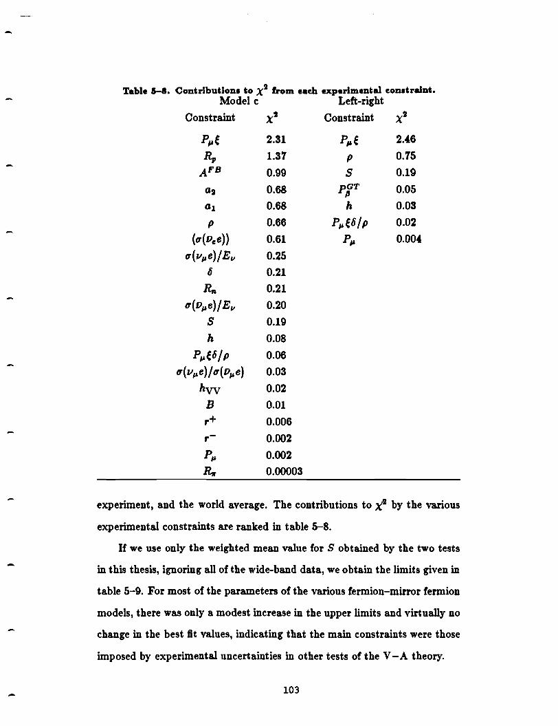
-
-
-
Table a-1. Contribution• to x2 from each experimental eon.tralnt. Model c Left-right
Constraint x2 Constraint x2
P11 ( 2.31 P11 ( 2.j6
R,, 1.37 p 0.75 AFB 0.99 s 0.19
a:1 0.68 pGT /J 0.05
a1 0.68 h 0.03
p 0.66 P,..(6/p 0.02
(D'(Oee)} 0.61 P,, 0.004
D'(v,..e)/ E11 0.25
6 0.21
Rn 0.21
D'(011e)/ E11 0.20
s 0.19
h 0.08
P11(6/p 0.06
D'(v11e) / D'( o,..e) 0.03
hvv 0.02
B 0.01 ,+ 0.006 ,- 0.002
P,.. 0.002
14 0.00003
experiment, and the world average. The contributions to x·2 by the various
experimental constraints are ranked in table 5-8.
If we use only the weighted mean value for S obtained by the two tests
in this thesis, ignoring all of the wide-band data, we obtain the limits given in
table 5-9. For most of the parameters of the various fermion-mirror fermion
models, there was only a modest increase in the upper limits and virtually no
change in the best ftt values, indicating that the main constraints were those
imposed by experimental uncertainties in other tests of the V -A theory.
103
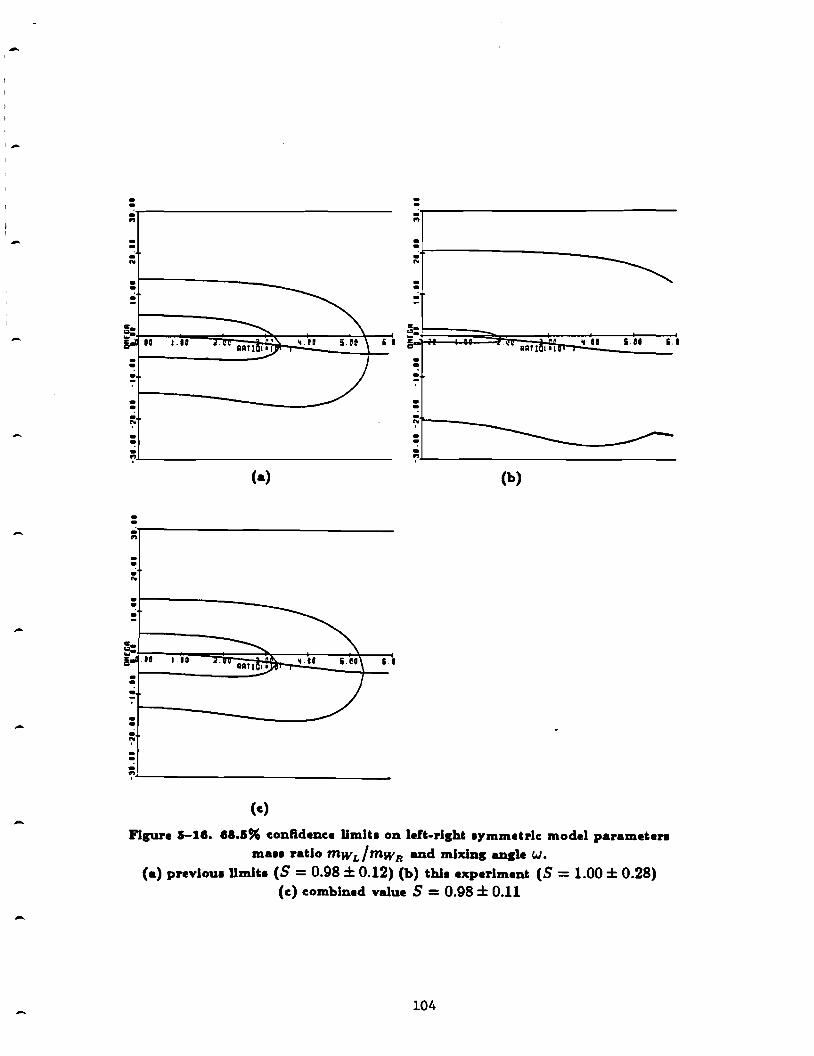
-
,_
-
-
-
-
- --. ......-~~~~~~~~~~~~~~~~-... ~ -.. --.; N
---.. _ ~-i aa I.ID . ~
~
. ~ . ... . ~ -... '
(•) (b)
. .
.; ...
. • . N
• • ~
... ::-! .u I 10 ' .. . ~
-• • . ... . ~ -':'
(c)
Figure 1-11. 18.1% confidence limlh OD left-right •)'mmetrlc model paramehn
maH ratio mw L / mw 8 and mixing angle w. (a) prevlou• limit• (S = 0.98 ± 0.12) (b) thl• experiment (S = 1.00 ± 0.28)
(e) eomblned value S = 0.98 ± 0.11
104
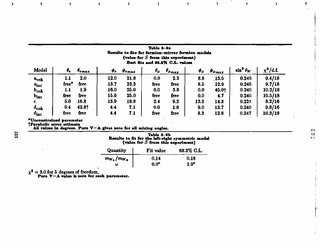
Table l-9a Re•u1'• 'o ftt• for fermion-mirror fermion modm
(value for S from thl• experlmmt) Be•i flt• and 18.1% C.L. valuff
Model Be Be mes f/>e fl>emas 9µ (JIAmu
"'"' fl> IA mu
&coh 1.1 2.0 12.0 21.8 0.0 2.3 8.8
8inc free* free 13.7 23.3 free free 8.5 hcoh 1.1 1.9 16.0 25.0 0.0 3.8 0.0 binc free free 15.9 25.0 free free 0.0 c 5.0 16.8 13.9 18.8 2.4 9.2 13.9 dcoh 0.4 42.8t 4.4 7.1 0.0 1.6 9.0 dine free free 4.4 7.1 free free 8.3
•uneo1Yiralned parameter · tParabolie error ••iimaie
All mu•• ID degre••· Pun V-A give• mero for all mbdng angl••·
Table 5-9b Re•uli• io Bi for the left-right •ymmeirle model
(value for S from ihl• experiment)
Quantity
mwL/mwR w .
x2 = 3.0 for 5 degrees of freedom. Pure V-A Ylllue l• uro for eaeb parameter.
Fit value
0.14 0.0°
68.3% C.L.
0.18 1.9°
13.5 -12.9 45.0t
4.7 14.3 13.7 12.8
sin2 9w
0.249 0.248 0.240 0.240 0.221 0.249 0.247
x' /d.f.
9.4/18 9.7/18
10.2/16 10.5/18 8.2/16 9.8/16
10.3/18
C\.1 (!)
(' l

-
-
CHAPTER VI. CONCLUSIONS
This concluding chapter will critique the studies of the inverse muon
decay that have been conducted to date, including the present experiment.
A few questions concerning the significance and reliability of the experimental
method used will be addressed.
The Gargamelle experiment1 obtained the E,,.B!/2me distribution shown
in figure 6-1. In this illustration, the background shape was measured by a
run taken with neutrinos at the CERN-PS below the threshold of inverse . muon decay. To apply this to the SPS run at energies over threshold, the
transverse muon momentum PT was assumed not to vary with neutrino en
ergy, and the parallel component of momentum was assumed to scale with
energy. The normalization of the background component was computed in
two ways. One was by comparing the number of events with PT > 160 MeV /c
for the PS run to that for the SPS run, and extrapolating to the range
PT < 160 MeV /c. The other was by means of a likelihood flt to the joint
distribution in E,,. and B! using theoretical densities for signal, quasielastic
scattering from nucleons, and quasielastic scattering from nuclei. The two
determinations of the relative normalization were in good agreement.
The advantage of using the low energy data to identify the quasielastic
component of the SPS results was that the nuclear effects must have been
the same for the two. The difference in the scanning efficiency was measured
and incorporated into the extrapolation.
The CHARM experiment2 used much the same method for detecting the
106

-
-
-
-
-
-·
-
-
lVENTS
PAEDICTION POlt
/vi'••· - 11··v• JO
I!
10
I
I
U DISTAllUTION FOA .. - IVIENTS
hie 14 CANDIDATIS
PAEmCTON FOR IACKGAOUND
• ·-IO IS
Figure 1-1. Gargamelle E62 /2me di•trlbutlon. (Ref. 1)
inverse muon decays in the Q2 distribution as the present experiment (fig
ure 6--2) except that because of the increased neutrino yield and live time in
the wide-band beam it was able to bin more finely in the low-Q2 region. The
cuts on the data relied mainly on scintillator pulse height response to mea
sure the amount of deposited energy near the vertex, which had sufficiently
fine resolution to distinguish one charged track from a number of charged
tracks. The region in Q2 above 0.1 GeV2 was neglected due to the difference
in recoilless neutrino and antineutrino acceptance there. No nuclear correc-
tion was made to eliminate the difference in the amount of Pauli suppression
for neutrinos and antineutrinos. The lack of such a correction would tend to
bias the results toward the V-A theory because of the dip in the antineu-
trino spectrum which is not the same as the one in the neutrino spectrum
(compare figure 5-4& to figures 5-4b through d as well as figure 2-1).
Data from the present experiment are displayed in the variables Q2 in
figure 5-4 and in E62 in figure 5-8. In the present experiment, due to the
107

-
-
-
.:-100
~ t
. ,._ ,.. e "' ~ z 41 ~ w -.. f z • ..
o o.o~ 0.1 .acGeY>1
Figure I-~. CHARM Q2 cll•tributlon•
limited number of events, the normalization of the Q2 distributions was over
a wider range, but the energy deposition cut was purposely left fairly loose
so as not to reject proton recoils from true quasielastics. Preliminary studies
using the proton recoil tracking package to discriminate against events that
had a clear recoil strongly aff'ected the result of subtracting the normalized
distributions, resulting in a much larger number of inverse muon decay events
than expected. To help show that something similar has not also happened
with the present set of filter cuts, the Monte Carlo neutrino and antineutrino
quasielastic spectra were subjected to the same analysis as the data. No
low-Q2 excess was found. A complementary analysis of the neutrino data,
subtracting the Monte Carlo quasielastic distribution for either neutrinos or
antineutrinos, yielded consistent results with the subtraction of the antineu
trino data. These are not compelling arguments as to the appropriateness
of the cuts, because of the limitations of the simulation used (which did not
take into account such eff'ects as scattering off' of entire nuclei, inelastic scat
tering, nuclear shell and spin eff'ects in quasielastic scattering, or noise hit
correlation in the calorimeter), but they do illustrate both the sensitivity of
108

-
-
-
-
the technique to differences between the data and the overall consistency of
the results.
Along the same lines, the consistency check provided by the differential
cross section test was interesting. This test did not depend at all on the
form of the nuclear corrections to the Q2 distribution, but gave answers
which agreed very well with the other tests. When the -165 data were flt
to the quasielastic scattering and inverse muon decay distributions in the
same manner as the positive train setting data, a null result for the excess
(N < 18.5 out of 311 total events, best flt N = 6.4) was observed at the
lu confidence level. This agreed with the additive conservation of lepton
number. In contrast, each of the positive train settings yielded best flt values
at least lu away from zero.
As for the theoretical analysis of the result, it must be pointed out here
how important it is to use approximations only in their appropriate range of
validity. As pointed out in more detail in Appendix A, the approximation
used by the CHARM experiment in deriving their expression for the differ
ential cross section :~ held only in the limit 1 > m! = 0.011 Ge V2• This
kinematic range cannot adequately represent the wide-band beam exposure
in the CERN-SPS (figure 3-1) which peaked at E11 = 20 GeV, corresponding
to • = 0.02 Ge V2 • The effect is to make the expected number of events for
pure V -A greater than the correct value and for pure V +A smaller than
the correct value. Of course, with a cross section linearly dependent on 1,
the effect of misrepresenting the part of the neutrino spectrum just above
the threshold energy (where the approximation is furthest from true) is less
significant than a similar error over all energies would be.
The limits on non-V-A couplings in the fermion-mirror fermion and
left-right symmetric models3 were still valid because the derivation of the
109
-
-
-
-
-
dependence on the inverse muon decay cross section did not use this approx
imation. One feature of this derivation which remains obscure was the origin
of the integration constant c which depended on the nature of the neutrino
energy spectrum. In analyzing the present data, it has not been altered from
its assigned value of 0.375, even though the neutrino spectrum was quite
different in most respects from that of the CERN-SPS beam.
In the future, when more precise measurements of such quantities as the
decay asymmetry e in direct muon decay will have been made, the inverse
muon decay cross section will be more significant in setting the best limits on
non-V-A couplings in the weak interactions. Limits on scalar, pseudoscalar,
and tensor couplings may be revised, in principle, in a fashion similar to that
of reference 3, although such a study was beyond the scope of the present
paper. Finally, in the higher range of B that will be available to the new
generation of accelerators, given sufficiently good statistics and sufficiently
good muon momentum resolution, the present analysis may well be extended
to future experiments in dichromatic neutrino beams. Depending on the
way in which any deviations from the usual V-A theory might arise, the
extension of this study to a higher center of mass energy range may make
certain departures from the usual V -A theory more prominent (e.g., due
to finite mass for the right-handed gauge boson in the left-right symmetric
model). The present level of knowledge concerning this topic is such that
there is still room for significant and physically relevant effects, whether
due to grand unification theories or for some other reason, to be observed
experimentally.
110
-
' -
-
-
-
-
APPENDIX A: DERIVATION OF CROSS SECTION:
The derivation of the cross section for the inverse muon decay
"" + e- ~ µ- + lie is given here in detail as a convenience for the reader to
make sense of a subject in disarray. The earliest treatment of the reaction1
gave a formula for the Hamiltonian that contained serious errors. Other
references2•3 give identical formulae for cross sections d du 8
but define the cos
same parameters differently. Owing to the confusion over whether the ap-
proximation 1 ± m! ~ 1 can be taken, one of these references3 has given an
inaccurate formula for : . None of the references delve into the details of
the Dirac algebra. Understanding the theoretical parameters, however, can
come only from seeing how the parameters derive from first principles.
The most general Hamiltonian density for this reaction containing only
V and A couplings is:
(A.l)
where gv and gA are the vector and axial vector complex coupling constants
and ""' e, p, and lie are spinors corresponding to each of the fermions. (This
is in "charge retention" ordering; it is related to "charge changing" ordering
Ei p(gi + ~"Y&)Oillp • OeO,e, which is familiar from the application of elemen
tary Feynman rules, by a Fierz transformation.~ This transformation would
introduce couplings i = S, P, A, V.) The square of the matrix element is
111

-
I ,_
'-I
-
given by
1 IMl2 = 2M2 (!"Y>.(l - "Ys)PIJ"Ya(l - "Yr,)e] w
· [Pµ"Y"(gv + gA"Y5)vePe"Ya(g~ + g~')'5)vµ] 1
= 2Ma, T1T2 (A.2)
where the mass of the intermediate vector boson Mw is included to approx
imate the full propagator, at the low center of mass energies typical of this
reaction. We can rewrite these factors in terms of traces:
(A.3)
where we have denoted the polarization vectors of the electron and of the
muon by •e and '"' the four-momenta of Vµ and Ve by p1 and P2, and
the initial neutrino beam polarization by P =: zi::l ~ zi:~l · Using the
identities
we have
"15(1- P"Y5hµ = - "Yµ(P + "15)
(1- ')'5) 2 =2(1- "15)
(1- "Y.s)(l + "Y.s) =O
Tr( odd number of "Yµ) =0
(A.4)
T1 =t Tr [(,Se+ me)(l - /eh.x(l - "Y.s)(pµ + mµ)(l - /µha(l - "Y.s)]
=!Tr [ (,S, + m,)( 1 - /.l1• ( (,Sµ + mµ/µh•( 1 - 1• )'
+ (mµ -,Sµ/µ)1.(1+1.)(1- 1s))]
=t Tr [(,Se - me/eh.x{pµ - mµ/µha(l - "Y.s)] (A.5)
112

-
-
r· t
T2 =Tr [,S11~'2'Y(T {(lgvl2 + lgAl2 ) + (gvg~ + gAg~)'Y5) (1 + P15)]
=(lavl2 + jgAl2) Tr [h1A,S21(T(l - .\-y5)(l + P-y5)]
where >. = -2Re(gyg~)
lllV 12 + jgA 12
(A.6)
and (A.7)
lav 12 + lgA 12
G} = gM,2 w
is the Fermi coupling constant. Reference 2 seems to disagree with both this
derivation and the formula in reference 3 on the sign of the parameter>.. We
can now use the identity5
to get
Tr ha'Y«T'Y,8")',.(a - fry5)) Tr ['Y"-y(T -y"-y" (c - d-y5)]
= 32ac [g~~ + g~g6] + 32bd [~g~ - g~g~]
IMl2 =4G} [32{i)(l - .1.Pl((p, + m,s,) · P1 (p. + m•••) · P2
+(Pe+ meae) · P2 (Pµ + mµaµ) · P1)
+ 32(i)(>. - P){(Pe + meae) ·Pi (Pµ + mµaµ) • P2
(A.8) .
-(p, + m,1,) · P2 [P• + m•••) · P1)] (A.9)
All the charged lepton polarization factors drop out when we average over Be
(picking up a factor of 1/2) and sum over Bµ. The Mandelstam variables may
now be incorporated:
I = (Pe + P1 )2 = m! + 2pe · P1
= (Pµ + P2)2 = m! + 2pµ · P2
t = (P1 - Pµ) 2 = m! - 2p1 · Pµ
= (Pe - P2 )2 = m~ - 2pe · P2
113
(A.10)

-
-
-
-
-
IMI' =8G} [11- lP) (1• - m!)(• - m!l + ll - m!)(t- m!l) .
+ ll - P) (I• - m:)(• - m!l - ll - m:)(t- m!J) ](A.11)
If we now neglect m~ with respect to 1, but keep m!,
IM/2 =8G} [11- lP + l-P)•I• - m!J
+ ll - >.P - H P)!ll - m!i]. In the center of momentum system,
8-m2
E1 = .jie =pi 2 8
1+m2
Eµ " 2.ji 1-m2
Pµ " 2.ji
t =m!- E1Eµ + 2p1pµcos8
_ _!_ [2m21 - 1
2 + m
21 - m
21 - m2
m2
- 21 " e " e "
+ (• - m:)(• - m!l cos6] 1
=2
, (1 - m~)(1 - m!)(l - cos8)
~i(1 -m!)(l - cos8)
(A.12)
(A.13)
where IJ is the angle between the muon direction and the incoming neutrino
direction.
IMI' =SG}•I• - m!l [11 + l)(l - P)
1 m 2
+ 4(1 - ..\)(1 + P)((l - 7)(1- cos8) + 2m!)
11- coa6)] (A.14)
114

-
-
dt1 =...!._(a - m~)(a - m~) IMl2
d cos 6 8a2 411' a
= ~6F (a - m!) {•(1 + ~)(1- P) 1 1ra
+ (1-,\)(1+ P) [1 + ~! - (1- m!) co•B]
x (1 - cos6)} (A.15)
This formula agrees with the formulae given by both reference 3 and refer
ence 2.
"" To arrive at the differential cross section du, we first need to set up
the kinematics in the center of momentum frame. Let the four-momentum
transfer be given by q = p1 - Pµ and let the unit 3-vectors x and .;t be in
the direction of the neutrino and of the muon respectively. If we start out
by leaving in all the charged lepton mass terms, we have
Pe: 27. (2m~ + 2E11me , -2E11mex)
q: &. (-m: - m! , (2E11m,)x - (m~ - m! + 2Evme).;f)
P1 :
Since cos 6 = x · .;t we have
m [ • Pe· q = 2
; 2E!m,(l - cosB) - E11m!(l + cosB)
- Evm!(l - cos8)- m: - m,m!]
. m [ = 2
; Ev(2Evme - m~)(l - cos6)
- Evm:(i + cos8) - m: - m,m!]
Pe· P1 = :, [4E!m: + 4E!m! + 4E!m!]
115
(A.16)

-
I-..
I_ I
-
= ;; (2E,,me(2E,, +me)] (A.17)
We can neglect the terms m!, mem!, and E,,m~(l + cos6) with respect to
the first term in the equation for Pe· q, each of which is down by at least six
orders of magnitude, and also neglect me with respect to E11 in the equation
for Pe · p1 • Then, since the inela.sticity II = Pe · q Pe · Pl we have
(1 m
2 ) 11 = - - "' (1 - cos 6)
2 4.meE11
=- - - -1!. (1 - cos6) 1 (1 m2
) 2 2 B
(A.18)
We apply the chain rule and substitute for (1 - cos 6) in the cross section:
get
dtT <UT ( du )-i dy = dcos6 dcos6
= G} (1 - m!) {4(1- P)(l +A) 161'1
+ (1 + P)(l - A) 2
'11
2 [a+ m! - a+ m! + 2sy]} 2' 2 B-m"' 1-m"'
= <7 (s - m!){(l + P)(l - A)y m! + ~11 + (1-P)(l + .\)}. (A.19) .. r s- mµ
A previous experiment3 takes a further approximation B :I: m~ Rl B to
dtT Rl G} B [(l + P)(l - A)y + (1 - P)(l - A)]. du '"'
(A.20)
This approximation is not valid in this experiment because for a reasonable
neutrino energy of 20 GeV, • Rl 0.02 GeV2 , m! = 0.011 GeV2 and the cross
section would be wrong by a. factor of 2.
116

-
1-
I_ I
APPENDIX B: DETERMINATION OF COUPLINGS FROM
THE INVERSE MUON DECAY RATE
This appendix is intended to give more details concerning the predictions
for the inverse muon decay rate on the basis of the theories mentioned in
section 3C of the text. It is essentially a condensation and reorganization of
the material in references I and 2.
BA. Fermion-mirror fermion mixing models.
Let us consider first the fermion-mirror fermion mixing model. The
charged leptonic current is:
where the conventional leptons are l' and ~ and the mirror leptons are L~
and N;. The primes are to distinguish the chirality states from the mass
eigenstates:
(B.2)
The angles flt and tPt are called mixing angles. We make the definitions
_ 2 cos( 8t + t/Jt) cos( 8t - tPt) Ot _____ ....>......,;;.._~'---~~__..;...;~
- cos2 (lh + cf>t) + cos2 (6t - cf>t) _ _ 2sin(8t + cf>t) sin(8t - tPt) Ot = 2 2
sin ( 6t + cf>t) + sin ( Bt - tPt) Pt Ecos26t (B.3)
The eft'ect of mirror fermion mixing upon the experimental tests that we have
chosen will depend on the masses of the mirror leptons. Since charged mirror
117
-
,_
) ,_
-
-
-
-
leptons lighter than about 20 Ge V / c2 are excluded by present experiments
in e+ e- rings, we need only consider the different mass scales for mirror
neutrinos. Ignoring, for our purposes, the third and any higher generations,
we have four special cases:
model m(Ne) m(Nµ) a <me <me b <me >mK c >mK >mK d >mK <me.
With respect' to inverse muon decay, two cases of models a, b, and d
may be distinguished. If the difference in masses between N" and vµ is small
(less than 1/2 e V) the neutrino beam and mirror neutrino beam will form
coherent weak eigenstates by the time it reaches the detector. If one goes
to the opposite extreme and assumes that the difference is on the order of
10 eV or so, then the oscillations will average incoherently at the detector.
We shall then speak only of the special "coherent" and "incoherent" cases
&cob' 8inc' bcoh' and binc ·
If we let cos(Dt - tf>t) =Vt,
cos(Dt + tf>t) =At, then the differential cross section is
sin(Dt - tf>t) =Vt,
sin(Dt + tf>t) =At
d4 =GJ.•{(V2 +A2 )(V2 +A2 )(2-211+1l- m!(2-11)) d11 161" e e µ µ I
+ f VeAe VµAµ ( 211 - y2 - ~! 11)
- 2P •• [ ( (V.' + A:Jv.A. + (V: + A~)V,A,) ( 1 - m;) + ( (Ve2 + A!)VµAµ - (V: + A~)VeAe)
(BA)
x (1-211+11'- mf (1-11)))} (B.5)
118

In experiments testing the integrated cross section, the inelasticity 1J and the
Mandelstam invariant s are averaged over the neutrino energy spectrum. The
cross section is then normalized by the pure V -A prediction for the reaction
to give a quantity that is called S. So, for the various fermion-mirror fermion
models, we have
Model
acoh S = t [(cos4 611 + sin4 611 )(1 + c)
+Pe( cos4 611 - sin 4 611 )(1 - c)]
8inc S = t(cos4 611 + sin4 9'>11 ) [(cos4 611 + sin4 611 )(1 + c)
+ Pe(cos4 611 - sin4 611 )(1 - c)]
b S = t [(1 + a~)(l + c) + 2Pea,i(l - c)]
c S = t [(1 + a~)(l + c) + 2aea11 (1- c)]
dcoh S = t [(cos4 611 + sin4 811 )(1 + c)
+ ae(cos4 6,i - sin4 6,i)(l - c)]
dine S = t(cos4 9'>11 + sin4 9'>11 ) [(cos4 811 + sin4 611 )(1 + c)
+ ae(cos4 611 - sin4 611 )(1 - c)] (B.6)
where c performs the average over the 1J terms in the cross sections. For
the CHARM experiment, c = 0.375, and this value was used for the present
experiment.
BB. Left-right symmetric models.
This model uses a charged current Lagrangian of the form
l!c = - g rn!Wl(Jr - Jf) +Wk( Jr+ Jf )) + h.c. (B.7) 2v2
where WL and WR are charged left- and right-handed spin-1 gauge boson
fields and the leptonic currents are Jl1e = l"'fKVt and Jf;K = l"YK"'f[,Vt· The
119

-
1,_
-
gauge particles will form eigenstates W1 and W2 with a mixing angle w
We now define
(:.1 ) = (c~s w - sin w) (:L)
2 smw cosw R
1 + tanw E=
1-tanw r+l'
'lAA = 1 + rE2
2 mw, r= 2
mw. _ (r - l)E
'lAV - 1 + rE2
(B.8)
{tcLR = g" [(sinw - cosw)9 + (sinw + cosw)
2] (B.9)
8 mw1 mw.
The differential cross section for inverse muon decay is then
(B.10)
and the normalized integrated cross section is
s = t (1 + '1AA)2
+ .,,~v + •P"; 'lAV ~12+ 'lAA) + c(l - '1AA)2
• (B.11) 1 + 'lAA + 'lAV
This depends on the parameters m(W1 )/m(W2) and w thr~ugh the parame
ters 'lAA and 'lAV.
BC. Models with more arbitrary couplings.
Reference 2 quotes the formula for the normalized, integrated cross sec
tion for inverse muon decay
S =2~ { (1 + c - 2c') [1Gsl2 + IG~l2 + jGpj2 + IG~l2
- 2P!l(GsG~ • + GpG~ *))
120
-
,_
I I_ I
-
+ 2(1+c+2c') [IGTl2 + IGTl2 - 2P~(GTGT *)]
-2(1- c) (~(GsGT + G~G1'* - GpQT- G~GT *)
-P~(GsG1' * + G~GT- GpG'-r* - G~GT)]
+ 2(1 + c) [IGv 1 2 +IG~12+IGA1
2+IG~1
2
+ 2P~(GvG~ *+GAG~*)]
+ 4(1- c) (~(GvGA + G~G~ *)
+ P~(GvG~ *+GAG~*)]} (B.12)
where c is the constant from averaging over the 11 distribution ( = 0.375 for
CHARM), c' is another constant of unspecified origin (= 0.5 for CHARM),
P is the neutrino handedness, and the various complex coefficients Ge are
coupling constants. The V-A limit is obtained when Gv =GA = 1, G~ = G~ = -1, and all other Ge constants are 0. The dimensionless parameter A
is related to the muon lifetime r,.,. as follows:
(B.13)
and is equal to 16 in the V-A case.
Owing to the lack of details on the derivation in reference 2, we shall not,
in this thesis, attempt to reproduce the limits on the S, P, .and T couplings
with our results on the inverse muon decay. It would be beyond the scope of
this work to derive a formula for the differential cross section : in the most
general case. This is what would be required to exploit properly the ability
to measure the 11 dependence of this reaction using a narrow-band neutrino
beam.
121

-
' -
I I_ '
-
APPENDIX C: CHARGE DIVISION READOUT
OF THE TOROID PROPORTIONAL CHAMBERS
In this appendix we shall describe the scheme which allowed us to deter
mine which among 4470 wires were hit in a given event, using only 720 am
plifier channels. ·
wires---- ---- -----1
1 2
1 1 i: n
1 R R R
AmP1 AmP2
Flpre C-t. Chars• dlvl•lon network.
In charge division, a group of adjacent wires are connected in parallel
using a resistive-capacitive network. (See figure C-1.) For two of the double
24' planes the wires were read out in groups of sixteen, using 680 resistors,
with an amplifier on each end. The other planes were read out in groups of
eight, with 1000 resistors. If we approximate these by the continuous case,
as a transmission line with constant resistance, inductance, and capacitance
per unit length, we obtain the telegrapher's equation.1 Solving this equation, 122
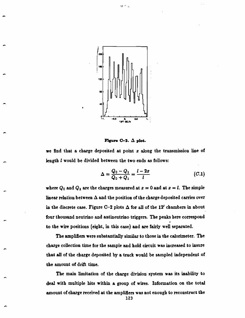
u , ..
(: I
120
IO
1
o~ i -1. -0.S a. o.a 1. '
12'1' DELTA
figure C-:a. 4 plot.
we find that a charge deposited at point z along the transmission line of
length l would be divided between the two ends as follows:
4 _ Qo -Qi __ l-_2_z - Qo +Q1 - l
(C.l)
where Qo and Q1 are the charges measured at z = 0 and at z = l. The simple
linear relation between 4 and the position of the charge deposited carries over
in the discrete case. Figure C-2 plots 4 for all of the 121 chambers in about
four thousand neutrino and antineutrino triggers. The peaks here correspond
to the wire positions (eight, in this case) and are fairly well separated.
The ampWlers were substantially similar to those in the calorimeter. The
charge collection time for the sample and bold circuit was increased to insure
that all of the charge deposited by a track would be sampled independent of
the amount of drift time.
The main limitation of the charge division· system was its inability to
deal with multiple bits within a group of wires. Information on the total
amount of charge received at the ampliB.ers was not enough to reconstruct the 123
-
-
-
-
·- ··- ---- ---------- - - - -- -- --b t1 {---·----- -·····-------··
hit locations, and the resolution was degraded. Multiple hits may have come
from delta-ray production in the toroid magnets, accidental coincidences with
cosmic rays or noise, or from multiple muons. On the whole, however, the
toroid spectrometer cuambers were able to give sufficieutly good momentum
resolution at moderate muon energies for the purposes of this thesis.
124
. -----------··-- ---------------8·~-:··---
LIST OF REFERENCES-Chapter 1.
1. W. Pauli, Proc. Solvay Congr. (1933), 324.
2. E. Fermi, Zeit. Pbys. 88 (1934), 161.
3. T. D. Lee and C. N. Yang, "Question of Parity Nonconservation in Weak Interactions," Pbys. Rev. 104 (1956), 254.
4. C. S. Wu et al., "Experimental Test of Parity Conservation in Beta Decay," Pb.ys. Rev. 105 (1957), 1413-1415.
125
-
-
LIST OF REFERENCES-Chapter 2
1. E. Commins, P. H. Bucksbaum, Weak Interactions of Leptons and Quarks, Cambridge: Cambridge University Press, 1983, p. 10.
2. H. Frauenfelder et al., Phys. Rev. 107 (1957), 643. P. Cavenagh et al., Pbil. Mag. 41 (1950), 701. A. de Shalit et al., Phys. Rev. 170 (1968), 1200.
3. M. Goldhaber et al., Phys. Rev. 109 (1958), 1015.
4. R. P. Feynman, M. Gell-Mann, Phys. Rev. 109 (1958), 193. R. Marshak, E. Sudarshan, Phys. Rev. 109 (1958), 1960.
5. F. Bergsma et al., "Experimental Study of the Reaction llµe- -+ µ-11e,'' Phys. Lett. 122B, (1983) 465-470.
Commins and Bucksbaum, op. cit. , p. 128.
6. L. Wolfenstein, "Lepton Number Violation and Neutrino Mass," CarnegieMellon University preprint CMU-HEP84-84.
7. M. L. Goldhaber et al., Phys. Rev. 109 (1958), 1015.
8. G. L. Kane, "Generalized Higgs physics and technicolor," Les Hooches Session XXXVII, 1981, Gauge Theories in High Energy Physics, Part I ed. Mary K. Gaillard and Raymond Stora, Amsterdam: North-Holland, 1983, pp. 415-440.
9. K. Mursula et al., "The Lorentz Structure of Leptonic Charged Weak Interactions," Noel. Phys. B219 (1983), 321-340.
10. J. Lovseth, "On the Angular Distribution of the Brookhaven 1962 Neu-trino Experiment," Phys. Lett. 6 (1963), 99-201. ·
11. T. Kitagaki et al., "High-energy quasielastic llµn -+ µ-p scattering in deuterium," Phys. Rev. D28 (1983) 436-442.
12. Y .-P. Yao, "Nuclear Effects on the Quasi-Elastic Neutrino Scattering 11 + n-+ µ- + p," Phys. Rev. 176 (1968), 1680-1685.
J. S. Bell, C. H. Llewellyn Smith, "Quasielastic Neutrino-Nucleus Interactions," Noel. Phys. B28 (1971), 317-340.
S. K. Singh, "The Effect of Final State Interactions and Deuteron Binding in 11 + d-+ µ-pp,"Nucl. Phys. B36 (1972), 419-435.
C.H. Llewellyn Smith, "Neutrino reactions at accelerator energies," Phys. Rep. a ( 1972), 310-313.
126

-13. B. Goulard, H. Primakoft', "Nuclear Structure Effects in 'Elastic' Neutrinoinduced Reactions," Phys. Rev. 135 (1964) Bll47.
14. D. H. Perkins, "Review 9f Neutrino Experiments," Proc. 19'15 Intl. Symp. on Lepton &IJd Photon Interactions at High Energies, Stanford: (1975), 575.
15. R. T. Ross, "A Study of the Reaction vp - µ- 7f+ p," Neutrmos-18, ed. E. C. Fowler, Purdue University, (1978), 929-938.
127
-
-
-
-
LIST OF REFERENCES-Chapter 3
1. N. Armenise et al., "Experimental Study of the Reaction 11,.,. + e- -+
µ- +lie,"' Phys. Lett. 84B (1979), 137-142.
2. M. Jonker et al., "Experimental Study of Inverse Muon Decay," Phys. Lett. 93B (1980), 203-209.
3. F. Bergsma et al., "Experimental Study of the Reaction 11,.,.e- -+ µ-11e," Phys. Lett. 122B (1988), 465-470.
4. A. N. Diddens et al., "A Detector for Neutral-Current Interactions of High-Energy Neutrinos," Noel. Instr. and Meth. 178 (1980) 27-48.
C. Bosio et al., "Proportional Drift Tubes for Large Calorimeter Detectors," Noel. Instr. and Meth. 157 (1978), 35-46.
5. J. Maalampi et al., "Study of the V, A Structure of the Charged Leptonic Current," Noel. Phys. B207 (1982), 233-250.
6. K. Mursula et al., "The Lorentz Structure of Leptonic Charged Weak Interactions," Noel. Phys. B219 (1983), 321-340.
1. K. Enqvist et al., "Mirror Leptons," Noel. Phys. B226, (1983), 121-151.
8. E. Di Capua et al., "Study of the Decay 1r -+ e + 11," Phys. Rev. 188 (1964), Bl333-Bl340.
D. Bryman, C. Picciotto, "Revised value for the tr -+ e11 branching ratio," Phys. Rev. Dll (1975), 1337.
9. K. S. Heard et al., "A Measurement of the (K+ -+ e+11)/(K+ -+ µ+11) Branching Ratio," Phys. Lett. 55B (1975), 327-330.
J. Heintze et al., "A New Measurement of the (K+-+ e+11)/(K+-+ µ+11) Branching Ratio," Phys. Lett. 60B,302-304.
10. R. Abela et al., "Measurements fo the polarization of the 2p and lB states in muonic atoms and helicity of the muon in pion decay," Noel. Phys. A 895 (1983), 413-434.
11. F. W. J. Koks, J. van KliDken, "Investigation on ~-Polarization at Low Velocities with ,8-Particles from the Decay of Tritium," Noel. Phys. A272 (1976), 61-81.
12. M.A. B. Beg et al., "Manifest Left-Right Symmetry and its Experimental Consequences," Phys. Rev. Lett. 88 (1977), 1252-1255.
128
-
-
,....
13. S. Derenzo, "Measurement of the Low-Energy End of the µ+ Decay Spectrum," Phys. Rev. 181 (1969), 1854-1866.
14. V. V. Akhmanov et al.," Asymmetry of Positrons from the Decay 7r+ -+
µ+ -+ e+ in the Longitudinal 140 000 Oe Magnetic Field," Sov. Joor. Noel. Phys. 6 (1968), 230-238.
15. F. Corriveau et al., "Measurement of the positron longitudinal polarization in muon decay," Phys. Rev. D24 (1981), 2004-2007.
16. F. Niebergall, Proc. Int. Cont. Neutrino '82, vol. 2, {Budapest, 1982), 62.
17. W. Bartel et al., "Observation of a Charge Asymmetry in e+e- -+
µ+µ-,"Phys. Lett. B108 {1982), 140-144.
18. A. Argento et al., "Electroweak Asymmetry in Deep Inelastic Muon Nucleon Scattering," Phys. Lett. 120B (1983), 245-250.
J. D. Bjorken, "Model-independent remarks on electron-quark parity-violating neutral current couplings," Phys. Rev. D18 (1976), 3239-3243.
19. J. Carr et al., "Search for Right-Handed Currents in Muon Decay," Phys. Rev. Lett. Sl, (1983), 627-630.
K. Mursula, "Leptonic Charged Weak Interactions in the Left-Right Symmetric Model," Noel. Phys. B241, (1984), 173-188.
20. D. P. Stoker et al., "Search for Right-Handed Currents by Means of Muon Spin Rotation," Phys. Rev. Lett. 54, (1985), 1887-1890.
129
-
- LIST OF REFERENCES-Chapter 4
1. F. E. Taylor et al., "The Construction and Performance of Large Flash Chambers,,, IEEE 7ransactions on Nucl. Sci. , NS-27 (1980), 30-37.
D. Bogert et al., "The Operation of a Large Flash Chamber Neutrino Detector at Fermilab,,, IEEE 7ransactions on Nucl. Sci. , NS-29 (1982), 363-367.
2. F. Sauli, "Principles of Operation of Multiwire Proportional and Drift Chambers,,, CERN report 77-00 (1077).
J. A. Jaros, "Drift and Proportional Tracking Chambers," SLAC-PUB-2647, (1080).
3. J. Boflll et al., "The Application of Resistive Charge Division in Large Proportional Tube Chambers," IEEE 7ransactions on Nucl. Sci. , NS-29, (1982), 400-401.
4. Particle Data Group, "Review of Particle Properties," Phys. Lett. lllB, {1982).
5. A. Mukherjee, "Shower Monte Carlo Versus Calibration," E594 internal memo 84-25, (1984).
6. R. Verdier, J. S. Whitaker, "Muon Tracking Package for E594 Offl.ine Analysis, Version 3" E594 internal memo 83-3, (1083).
7. J. Boflll, "Upper Limit for Vµ. Oscillation into vf' in a Dichromatic Beam," Ph.D. thesis, Massachusetts Institute of Technology, (unpublished), (1984), p. 56.
8. Ibid., p. 34.
130

-
LIST OF REFERENCES-Chapter 5
1. J. Maalampi, et al., "Study of the V, A Structure of the Charged Leptonic Current," Nucl. Phys. B 201 (1982), 233-250.
2. T. Eldridge, private communication.
3. W. T. Eadie et al., Statlstlcal Methods ln Experimental Phy1lc1, (London: North-Holland, 1971), 257-262.
4. J. Boflll, Ph.D. thesis, Massachusetts Institute of Technology, 1984, (unpublished).
5. J. Orear, "Notes on Statistics for Physicists, Revised," Cornell University preprint CLNS 82/511, July 1982.
6. F. Bergsma et al., "Experimental Study of the Reaction vµe- ~ µ.-v,:," Phys. Lett. 122B (1983), 465-470.
7. R. Pitt, "Current State of E-594 Narrow Band Flux Analysis," E594 internal memo 84-24, (1984).
8. F. E. Taylor, "The Weight of the Calorimeter," E594 internal memo 83-8 (1983).
131
-
-
-
-
-
,...
LIST OF REFERENCES-Chapter 6
1. N. Armenise et al., "Experimental Study of the Reaction llµ + e- ....,. µ- +lie," Phys. Lett. 84B (1979), 137-142.
2. M. Jonker et al., "Experimental Study of Inverse Muon Decay," Phys. Lett. 9SB (1980), 203-209.
F. Bergsma et al., "Experimental Study of the Reaction llµe- ....,. µ-lie," Phys. Lett. 122B (1983), 465-470.
3. J. Maalampi et al., "Study of the V, A Structure of the Charged Leptonic Current," Noel. Phys. B201 (1982), 233-250.
4. K. Mursula et al., "The Lorentz Structure of Leptonic Charged Weak Interactions," Nucl. Phys. B219 (1983), 321-340.
132
-
-
LIST OF REFERENCES-Appendix A
1. C. Jarlskog, "Tests of the V-A Theory in Neutrino-Lepton Interactions," Lett. al Nuov. Cim. 8, {1970), 377-380.
2. N. Armenise et al., "Experimental Study of the Reaction Vµ + e- -+ µ- +Ve,'' Phys. Lett. 84B, (1979), 137-142.
3. F. Bergsma et al., "Experimental Study of the Reaction Vµ + e- -+ µ- +Ve," Phys. Lett. 1228, {1983), 465-470.
4. F. Scheck, Leptons, Hadrons, and Nuclei. Amsterdam: NorthHolland, 1983.
5. E. D. Commins, P. H. Bucksbaum, Weak Interactions of Leptons and Quarks, Cambridge: Cambridge University Press, 1983, p. 95.
133
-
LIST OF REFERENCES-Appendix B
1. J. Maa.lampi et al., "Study of the V, A Structure of the Charged Leptonic Current," Nucl. Phys. B207 (1982), 233-250.
2. K. Mursula et al., "The Lorentz Structure of Leptonic Charged Weak Interactions," Nucl. Phys. B219 (1983), 321-340.
134
-
LIST OF REFERENCES-Appendix C
1. M. G. Forrester, B.S. thesis, Massachusetts Institute of Technology, June 1981 (unpublished) ..
J. L. Alberi, V. Radeka, "Position Sensing by Charge Division," IEEE 7raDs. OD Nucl. Sci., Vol. NS-23, 1976.
V. Radeka, P. Rehak, "Charge Dividing Mechanism on Resistive Electrode in Position-sensitive Detectors," IEEE 7rans. OD Nucl. Sci., Vol. NS-26, 1979.
135
-
-
ACKNOWLEGMENTS
I would like to take this opportunity to thank the many individuals
who made my work possible. To the senior members of the Counter Spark
Chamber Group at I\..fiT I owe a great deal more than just my livelihood
these last 6.ve years; if I have learned anything about how to run a large
scale experiment, I have learned it from Wit Busza, Larry Rosenson, Lou
Osbome, Scott Whittaker, Jerry Friedman, and, especially, from my adviser,
Henry Kendall. I extend to them my gratitude. A list of credits would
be incomplete without mention of the special contributions, technical and
non-technical, of the redoubtable Tommy Lyons. Without his ideas, this
experiment would have been somewhat impoverished.
Day in and day out, my fellow graduate students provided both the best
possible way to leam physics (and a lot besides physics, I should add) and a.
great bunch of friends in a living and working situation that only those who
have experienced it can know about. I would like to list all the ways they
contributed to the experiment and to me personally, but I do not have the
space here. Many thanks to Juan Boflll, Andy Cohen, Terry Eldridge, Tom
Mattison, Aseet Mukherjee, Mike Tartaglia, John Slate, and Gong Ping Yeh.
I would like to thank the other members of the E594 experiment for their
assistance and hard work: from Michigan State University, Maris Abolins,
Dan Owens, Chip Brock, and Harry Weerts; from Fermifab, Linda Stutte,
Dixon Bogert, Jorge Morfin, and Jimmy Walker; and from MIT, Robin
Verdier, Stu Fuess, Maury Goodman, and Randy Pitt. In particular, I greatly appreciate the encouragement and advice from Frank Taylor relating to this
thesis. To the staffs of the Users' and Housing Offices at Fermilab and of the
Laboratory of Nuclear Science at MIT, many thanks. I am deeply indebted
to the super administrative assistants who kept things running at MIT, Sally Anand and Sandy Spry, for service in ways too numerous to list.
Without the support of my extended family I would never have been able to complete this work. My steadfast friends at the Tech Catholic Community
136

-
-
taught me by example how even a big university can excel in humanity; to
Christian, Luz, Mary Jean, Sue, and to so many others, I give my heartfelt
thanks. The parish of St. John Neumann in St. Charles was a lifeline for me,
as well as an inspiration. Through all the trials of my graduate career, my
pastors, Bob Moran, Dan Hermes, and Bob O'Donnell have led me safely and
I give them my thanks. I am deeply grateful to Virginia S. Finn for the many
ways she has been present to me, as friend, counselor, and family. To my
own family I owe the greatest debt of thanks: to my mother, Mariquita, to
my father, Carlos, for always encouraging me in whatever vocation I should
choose, to my sister, Cheryl, for her constant concern and thoughtfullness,
and, most of all, to my bride-to-be, Pam, for giving of herself in every way,
I give my love and gratitude.
137