observational aspects of hard x-ray polarimetry
TRANSCRIPT

Observational Aspects of Hard X-ray
Polarimetry
A thesis submitted in partial fulfilment of
the requirements for the degree of
Doctor of Philosophy
by
Tanmoy Chattopadhyay
(Roll No. 11330008)
Under the guidance of
Dr. Santosh V. Vadawale
Associate Professor
Astronomy & Astrophysics Division
Physical Research Laboratory, Ahmedabad, India.
DISCIPLINE OF PHYSICS
INDIAN INSTITUTE OF TECHNOLOGY GANDHINAGAR
2015


to
my family


Declaration
I declare that this written submission represents my ideas in my own words
and where others’ ideas or words have been included, I have adequately cited and
referenced the original sources. I also declare that I have adhered to all principles
of academic honesty and integrity and have not misrepresented or fabricated or
falsified any idea/data/fact/source in my submission. I understand that any
violation of the above will be cause for disciplinary action by the Institute and
can also evoke penal action from the sources which have thus not been properly
cited or from whom proper permission has not been taken when needed.
(Signature)
(Name: Tanmoy Chattopadhyay)
(Roll No: 11330008)
Date: November 26, 2015


CERTIFICATE
It is certified that the work contained in the thesis titled “Observational
Aspects of Hard X-ray Polarimetry” by Mr. Tanmoy Chattopadhyay
(Roll No. 11330008), has been carried out under my supervision and that this
work has not been submitted elsewhere for a degree.
Dr. Santosh V. Vadawale
(Thesis Supervisor)
Associate Professor,
Astronomy & Astrophysics Division
Physical Research Laboratory,
Ahmedabad, India.
Date:


i
Acknowledgements
First and foremost, I would like to express my sincere gratitude to my advisor
Dr. Santosh Vadawale for his continuous support in my Ph.D study and related
research. His guidance helped me throughout the time of PhD and writing of this
thesis.
Besides my advisor, I would like to thank the rest of my thesis committee:
Prof. N. M. Ashok, Prof. Janardhan Padmanabhan, and Dr. Sachindra Naik,
for their insightful comments and encouragement.
My sincere thanks also goes to Prof. A. R. Rao, Prof. Dipankar Bhattacharya,
who provided me an opportunity to join Astrosat-CZTI team, giving me access to
the laboratory and research facilities. Without their precious support it would not
be possible to conduct this research. I would like to thank other team members of
the CZTI team Dr. Varun Bhalerao, Rasika, Pramod, Kutty, Malkar sir, Amir,
Anish, Nilkanth, Rakesh, Mithun and others for their continuous support in my
research work in PRL, TIFR and IUCAA.
I would like to thank all the faculty members in Astronomy & Astrophysics di-
vision, PRL, specially Prof. B. G. Anandrao, Prof. T. Chandrasekhar, Dr. Ashok
Singal, Prof. U. C. Joshi, Prof. H. O. Vats, Prof. N. M. Ashok, Prof. D. P.
K. Banerjee, Prof. P. Janardhan, Prof. K. S. Baliyan, Dr. A. Chakraborty, Dr.
Sachindra Naik, Dr. S. Ganesh, Dr. Mudit Srivastava and Dr. V. Venkataraman
for their useful comments and suggestions and continuous support during my PhD
tenure.
I thank my fellow labmates in PRL − Mr. Shanmugam M., Mr. Shivku-
mar Goyal, Mithun, Rishab, Arpit, Tinkel, Mr. A. B. Shah and others for the
stimulating discussions and helping me out in my research work.
Also I thank my batchmates and friends for their continuous support and all
the fun we have had in the last five years. I am grateful to Priyanka, Arko,
Monojit, Balaji, Pragya and Golu, Naveen, Sneha, Shweta and others for spending
valuable time with me in the last five years, which I will cherish throughout my life.
I take this opportunity to thank my B.Sc. and M.Sc. batchmates and friends −Rupomoy, Abhisek, Sudip, Rajib, Dhrubo, Debraj, Someswar, Kousik K., Kousik
B., Tanmoy R., Suman, Saptorshi, Abhivav, Avdesh, Mayukh da, Aniruddha da,
Biswarup, Sibu, Jitu, Bablu who had directly and indirectly helped me achieved
this goal.
I am grateful to Prof. Hiralal Yadav in B.H.U., Prof. Bhabani Prasad Mandal
in B.H.U., and Prof. Ashok Banerjee in T.D.B. college for enlightening me the
first glance of research. I am thankful to all my teachers especially Amitabha sir

ii
and Phonibhusan sir for teaching me not only the academic subjects but also the
important lessons in life.
Last but not the least, I would like to thank my family: my parents and to my
sisters for their encouragement, support and attention throughout my life.
(Tanmoy Chattopadhyay)

iii
Abstract
Sensitive polarization measurements in X-ray may address a wealth of as-
trophysical phenomena, which so far remain beyond our understanding through
available X-ray spectroscopic, imaging, and timing studies. Though scientific
potential of X-ray polarimetry was realized long ago, there has not been any
significant advancement in this field for the last four decades since the birth of
X-ray astronomy. The only successful polarization measurement in X-rays dates
back to 1976, when a Bragg polarimeter onboard OSO-8 measured polarization
of Crab nebula. Primary reason behind the lack in progress is its extreme photon
hungry nature, which results in poor sensitivity of the polarimeters.
Recently, in the last decade or so, with the advancement in detection technol-
ogy, X-ray polarimetry may see a significant progress in near future, especially
in soft X-rays with the invention of photoelectron tracking polarimeters. Though
photoelectric polarimeters are expected to provide sensitive polarization mea-
surements of celestial X-ray sources, they are sensitive only in soft X-rays, where
the radiation from the sources is dominated by thermal radiation and therefore
expected to be less polarized. On the other hand, in hard X-rays, sources are ex-
pected to be highly polarized due to the dominance of nonthermal emission over
its thermal counterpart. Moreover, polarization measurements in hard X-rays
promises to address few interesting scientific issues regarding geometry of corona
for black hole sources, emission mechanism responsible for the higher energy peak
in the blazars, accretion geometry close to the magnetic poles in accreting neutron
star systems and acceleration mechanism in solar flares. Compton polarimeters
provide better sensitivity than photoelectric polarimeters in hard X-rays with a
broad energy band of operation. Recently, with the development of hard X-ray
focusing optics e.g. NuSTAR, Astro-H, it is now possible to conceive Comp-
ton polarimeters at the focal plane of such hard X-ray telescopes, which may
provide sensitive polarization measurements due to flux concentration in hard
X-rays with a very low background. On the other hand, such a configuration
ensures implementation of an optimized geometry close to an ideal one for the
Compton polarimeters. In this context, we initiated the development of a fo-

iv
cal plane Compton polarimeter, consisting of a plastic scatterer surrounded by
a cylindrical array of CsI(Tl) scintillators. Geant−4 simulations of the planned
configuration estimates 1% MDP for a 100 mCrab source in 1 million seconds of
exposure. Sensitivity of the instrument is found to be critically dependent on the
lower energy detection limit of the plastic scatterer; lower the threshold, better
is the sensitivity. In the actual experiment, the plastic is readout by a photomul-
tiplier tube procured from Saint-Gobain. We carried out extensive experiments
to characterize the plastic especially for lower energy depositions. The CsI(Tl)
scintillators are readout by Si photomultipliers (SiPM). SiPMs are small in size
and robust and therefore provide the compactness necessary for the designing
of focal plane detectors. Each of the CsI(Tl)-SiPM systems was characterized
precisely to estimate their energy threshold and detection probability along the
length of the scintillators away from SiPM. Finally, we integrated the Compton
polarimeter and tested its response to polarized and unpolarized radiation and
compared the experimental results with Geant−4 simulation.
Despite the growing realization of the scientific values of X-ray polarimetry
and the efforts in developing sensitive X-ray polarimeters, there has not been a
single dedicated X-ray polarimetry mission planned in near future. In this sce-
nario, it is equally important to attempt polarization measurements from the
existing or planned instruments which are not meant for X-ray polarization mea-
surements but could be sensitive to it. There have been several attempts in past
in retrieving polarization information from few of such spectroscopic instruments
like RHESSI, INTEGRAL-IBIS, INTEGRAL-SPI. Cadmium Zinc Telluride Im-
ager (CZTI) onboard Astrosat, India’s first astronomical mission, is one of such
instruments which is expected to provide sensitive polarization measurements for
bright X-ray sources. CZTI consists of 64 CZT detector modules, each of which
is 5 mm thick and 4 cm × 4 cm in size. Each CZT module is subdivided into 256
pixels with pixel pitch of 2.5 mm. Due to its pixelation nature and significant
Compton scattering efficiency at energies beyond 100 keV, CZTI can work as a
sensitive Compton polarimeter in hard X-rays. Detailed Geant−4 simulations
and polarization experiments with the flight configuration of CZTI show that
v
CZTI will have significant polarization measurement capability for bright sources
in hard X-rays.
CZTI is primarily a spectroscopic instrument with coded mask imaging. To
properly utilize the spectroscopic capabilities of CZT detectors, it is important
to generate accurate response matrix for CZTI, which in turn requires precise
modelling of the CZT lines shapes for monoenergetic X-ray interaction. CZT
detectors show an extended lower energy tail of an otherwise Gaussian line shape
due to low mobility and lifetime of the charge carriers. On the other hand, inter-
pixel charge sharing may also contribute to the lower energy tail making the line
shape more complicated. We have developed a model to predict the line shapes
from CZTI modules taking into account the mobility and lifetime of the charge
carriers and charge sharing fractions. The model predicts the line shape quite
well and can be used to generate pixel-wise response matrix for CZTI.
Keywords: X-ray polarimetry, Compton scattering, Hard X-ray telescopes,
Geant−4 simulation, Instrumentation, Astrosat, Cadmium Zinc Telluride Imager
(CZTI), Response matrix, Cygnus X-1, Crab pulsar.


Contents
Acknowledgements i
Abstract iii
Contents vii
List of Figures xi
List of Tables xv
1 Introduction 1
1.1 Science Drivers for X-ray Polarimetry . . . . . . . . . . . . . . . . 3
1.2 X-ray Polarization Measurement . . . . . . . . . . . . . . . . . . . 10
1.2.1 Scattering polarimetry . . . . . . . . . . . . . . . . . . . . 12
1.2.2 Photoelectric polarimetry . . . . . . . . . . . . . . . . . . 14
1.2.3 Bragg reflection polarimetry . . . . . . . . . . . . . . . . . 15
1.3 Hard X-ray Polarimetry − How and Why : Thesis Overview . . . 15
2 Polarimetric Sensitivity of a Focal Plane Hard X-ray Compton
Polarimeter 21
2.1 Proposed Detector Configuration . . . . . . . . . . . . . . . . . . 22
2.1.1 Comparison with contemporary hard X-ray polarimeters . 23
2.1.2 Simulation and data analysis . . . . . . . . . . . . . . . . . 25
2.2 Semi-analytic Calculation of Modulation Factor and Efficiency . . 28
2.3 Polarimetric Sensitivity of CXPOL . . . . . . . . . . . . . . . . . 32
2.3.1 Spurious events calculation . . . . . . . . . . . . . . . . . . 32
vii

viii CONTENTS
2.4 Results and Discussions . . . . . . . . . . . . . . . . . . . . . . . 33
2.5 Summary . . . . . . . . . . . . . . . . . . . . . . . . . . . . . . . 36
3 Development of the Focal Plane Compton Polarimeter 37
3.1 Characterization of the Plastic Scatterer . . . . . . . . . . . . . . 38
3.2 Description of the Experiment . . . . . . . . . . . . . . . . . . . . 40
3.2.1 Experiment setup . . . . . . . . . . . . . . . . . . . . . . . 40
3.2.2 Results . . . . . . . . . . . . . . . . . . . . . . . . . . . . . 44
3.3 Numerical Modeling . . . . . . . . . . . . . . . . . . . . . . . . . 50
3.4 Modeling Results and Discussions . . . . . . . . . . . . . . . . . . 56
3.5 Characterization of CsI(Tl) Scintillators . . . . . . . . . . . . . . 62
3.6 Polarization Experiment with CXPOL . . . . . . . . . . . . . . . 68
3.7 Discussions and Future Plans . . . . . . . . . . . . . . . . . . . . 74
3.8 Summary . . . . . . . . . . . . . . . . . . . . . . . . . . . . . . . 76
4 Prospects of Hard X-ray Polarimetry with Astrosat-CZTI 79
4.1 Compton Polarimetry with Pixelated Detectors . . . . . . . . . . 81
4.2 Multi-pixel Detection Capability of CZTI Detector Modules . . . 83
4.2.1 Experiment setup . . . . . . . . . . . . . . . . . . . . . . . 83
4.2.2 Data analysis and results . . . . . . . . . . . . . . . . . . . 84
4.3 Geant−4 Simulation . . . . . . . . . . . . . . . . . . . . . . . . . 88
4.3.1 Estimation of polarimetric efficiency . . . . . . . . . . . . 89
4.3.2 Estimation of modulation factor . . . . . . . . . . . . . . . 92
4.4 Polarimetric Sensitivity of CZTI . . . . . . . . . . . . . . . . . . . 98
4.4.1 Source count rate . . . . . . . . . . . . . . . . . . . . . . . 98
4.4.2 Background estimation . . . . . . . . . . . . . . . . . . . . 98
4.4.3 Results . . . . . . . . . . . . . . . . . . . . . . . . . . . . . 103
4.5 Experimental Confirmation . . . . . . . . . . . . . . . . . . . . . 106
4.6 Astrophysical significance of CZTI Polarimetry . . . . . . . . . . . 108
4.7 Summary . . . . . . . . . . . . . . . . . . . . . . . . . . . . . . . 113
5 Generation of Multi-Pixel Response Matrix for Astrosat-CZTI 115
5.1 CZT Line Model . . . . . . . . . . . . . . . . . . . . . . . . . . . 117

CONTENTS ix
5.2 Measurements of µτ Products and Charge Sharing Fractions . . . 122
5.3 Verification of CZT Line Model: Crosstalk Experiment . . . . . . 126
5.4 Discussions and Future Plans . . . . . . . . . . . . . . . . . . . . 131
6 Summary and Scope for Future Work 133
6.1 Scope for Future Work . . . . . . . . . . . . . . . . . . . . . . . . 134
6.1.1 Solar X-ray polarimeter for future solar missions . . . . . . 134
6.1.2 Simultaneous spectroscopy, timing, imaging and polarimetry135
6.1.3 CZTI polarimetry for bright X-ray sources . . . . . . . . . 136
Bibliography 139
List of publications 161
Publications attached with thesis 163


List of Figures
1.1 Polarization characteristics for various black hole coronal geometries 4
1.2 Phase resolved optical polarimetry of Crab pulsar . . . . . . . . . 8
1.3 Spatially integrated flux and polarization for solar flares . . . . . 10
2.1 Planned configuration of the focal plane Compton Polarimeter
(CXPOL) . . . . . . . . . . . . . . . . . . . . . . . . . . . . . . . 23
2.2 A sample modulation curve obtained from simulation of CXPOL . 27
2.3 Schematic view of CXPOL scattering geometry . . . . . . . . . . 29
2.4 Modulation factor, polarimetric efficiency and figure of merit of
CXPOL . . . . . . . . . . . . . . . . . . . . . . . . . . . . . . . . 31
2.5 Polarimetric sensitivity of CXPOL as function of source intensity 34
2.6 Polarimetric sensitivity of CXPOL as a function observed energy . 35
3.1 LogN-LogS plot obtained from Swift BAT 70 month hard X-ray
survey . . . . . . . . . . . . . . . . . . . . . . . . . . . . . . . . . 39
3.2 Deposited energy in Compton scattering as a function of scattering
angle and photon energy . . . . . . . . . . . . . . . . . . . . . . . 42
3.3 Schematic view of plastic characterization experiment . . . . . . . 43
3.4 Block schematic for the coincidence unit between plastic scintilla-
tor and X123CdTe . . . . . . . . . . . . . . . . . . . . . . . . . . 44
3.5 CdTe detector spectra of the plastic scattered photons at different
scattering angles . . . . . . . . . . . . . . . . . . . . . . . . . . . 45
3.6 Rate of plastic scattered photons as collected by CdTe detector at
different scattering angles . . . . . . . . . . . . . . . . . . . . . . 48
xi

xii LIST OF FIGURES
3.7 Normalized plastic scattered photons as collected by CdTe detector
at different scattering angles . . . . . . . . . . . . . . . . . . . . . 49
3.8 Geometric representation of the experimental setup for plastic char-
acterization . . . . . . . . . . . . . . . . . . . . . . . . . . . . . . 51
3.9 Fitting of the normalized plastic scattered events as a function of
scattering angle by numerical model . . . . . . . . . . . . . . . . . 57
3.10 Comparison between experimentally obtained coincidence count
rate and modelled count rate assuming 100% detection probability
of plastic . . . . . . . . . . . . . . . . . . . . . . . . . . . . . . . . 58
3.11 Detection Probability of plastic scintillator as function of deposited
energy in plastic for 59.5 keV and 22.2 keV incident photons . . . 59
3.12 Detection probability of plastic as a function of deposited energy
from 0.4 keV to 10 keV . . . . . . . . . . . . . . . . . . . . . . . . 60
3.13 Polarimetric sensitivity of CXPOL after including plastic detection
probability . . . . . . . . . . . . . . . . . . . . . . . . . . . . . . . 62
3.14 Animated picture of the final CXPOL configuration . . . . . . . . 63
3.15 CsI(Tl) and SiPM assembly . . . . . . . . . . . . . . . . . . . . . 64
3.16 Schematic of the SiPM electronic readout system . . . . . . . . . 65
3.17 Spectra obtained from CsI(Tl)-SiPM system and detection proba-
bility of the system as function of interaction depth . . . . . . . . 66
3.18 Schematic view of the coincidence unit in CXPOL and the final
experimental configuration of CXPOL . . . . . . . . . . . . . . . 69
3.19 Response of CXPOL to unpolarized radiation . . . . . . . . . . . 70
3.20 Response of CXPOL to partially polarized monoenergetic radiation 71
3.21 Polarization experiment with CXPOL using partially polarized
continuum radiation from X-ray gun . . . . . . . . . . . . . . . . 73
3.22 Response of CXPOL to partially polarized continuum radiation . 74
4.1 The assembled CZTI payload onboard Astrosat . . . . . . . . . . 81
4.2 A single CZTI module procured from Orbotech Medical Solutions 82
4.3 Schematic diagram of the 57Co experiment setup with CZTI de-
tector module . . . . . . . . . . . . . . . . . . . . . . . . . . . . . 84

LIST OF FIGURES xiii
4.4 Time interval distribution for all successive events recorded in
CZTI module . . . . . . . . . . . . . . . . . . . . . . . . . . . . . 85
4.5 Raw double pixel spectra obtained from CZTI experiment . . . . 86
4.6 Double pixel spectra obtained from CZTI experiment after apply-
ing filtering conditions . . . . . . . . . . . . . . . . . . . . . . . . 87
4.7 Schematic view of a single CZT detector module obtained from
simulation . . . . . . . . . . . . . . . . . . . . . . . . . . . . . . . 88
4.8 Probability of single pixel, double pixel and beyond double pixel
events as a function of photon energies . . . . . . . . . . . . . . . 90
4.9 Cotribution of various interaction processes in generating double
pixel events in CZT detectors . . . . . . . . . . . . . . . . . . . . 90
4.10 Double spectra obtained from simulation of 200 keV beam with
CZTI for various interaction processes . . . . . . . . . . . . . . . 91
4.11 Azimuthal angle distribution for simulation of 200 keV beam with
CZTI for ideal Compton events and all double pixel events . . . . 92
4.12 Double pixel spectra and azimuthal angle distribution obtained
from simulation of 200 keV beam with CZTI with all filtering con-
ditions . . . . . . . . . . . . . . . . . . . . . . . . . . . . . . . . . 93
4.13 Ratio of Compton scattered photon energy to electron recoil energy
as a function of scattering angle and incident photon energies . . . 94
4.14 Deposited energy in Compton scattering as a function of scattering
angle and incident photon energies . . . . . . . . . . . . . . . . . 95
4.15 Simulated modulation curves for CZTI at various polarization angles 96
4.16 Modulation factor, polarimetric efficiency and figure of merit as a
function of photon energy for CZTI as estimated from simulation 97
4.17 Polarimetric background for CZTI . . . . . . . . . . . . . . . . . . 103
4.18 CZTI polarimetric sensitivity as a function of source intensity . . 104
4.19 Polarization experiment setup for CZTI . . . . . . . . . . . . . . . 106
4.20 Azimuthal angle distribution for a single CZTI module obtained
from polarization experiment . . . . . . . . . . . . . . . . . . . . . 107

xiv LIST OF FIGURES
4.21 Polarization detection significance with CZTI as function of expo-
sure time . . . . . . . . . . . . . . . . . . . . . . . . . . . . . . . . 109
4.22 Prospects of hard X-ray polarimetry of Cygnus X-1 and Crab with
Astrosat-CZTI . . . . . . . . . . . . . . . . . . . . . . . . . . . . 112
5.1 Demonstration of tailing effect in CZT line shape due to charge
trapping (µτ model) for 122 keV photons . . . . . . . . . . . . . . 118
5.2 Model predicted CZT line profiles as a function of charge cloud
radius (r0) . . . . . . . . . . . . . . . . . . . . . . . . . . . . . . . 120
5.3 Energy distribution for 59.54 keV and 122 keV photons obtained
from simulation . . . . . . . . . . . . . . . . . . . . . . . . . . . . 122
5.4 OMS Detectors Array Unit and the data collection unit OMS36G256-
SDK . . . . . . . . . . . . . . . . . . . . . . . . . . . . . . . . . . 123
5.5 Simultaneous fitting of CZT spectra at three different energies with
the numerical CZT line model . . . . . . . . . . . . . . . . . . . . 124
5.6 Distribution of (µτ)e and (µτ)h with pixels for CZT detector . . . 125
5.7 Distribution of initial charge cloud radius (r0) with pixels for CZT
detector . . . . . . . . . . . . . . . . . . . . . . . . . . . . . . . . 126
5.8 Experiment setup for Crosstalk experiment . . . . . . . . . . . . . 127
5.9 Count rate for 241Am as a function of source-slit position . . . . . 128
5.10 Count rate for 57Co as a function of source-slit position . . . . . . 129
5.11 Simultaneous fitting of six spectra obtained by illuminating differ-
ent parts of a pixel with a narrow slit . . . . . . . . . . . . . . . . 130

List of Tables
2.1 CXPOL scattering geometry dimensions . . . . . . . . . . . . . . 24
4.1 Polarimetric Sensitivity of CZTI . . . . . . . . . . . . . . . . . . . 105
4.2 List of potential sources for CZTI polarimetry obtained from BAT
70 month catalog . . . . . . . . . . . . . . . . . . . . . . . . . . . 113
xv


Chapter 1
Introduction
X-ray astronomy, a branch of astrophysics, deals with the detection of high en-
ergy electromagnetic radiation from celestial astrophysical sources. Since high
energy photons or X-rays do not reach the surface of earth owing to absorption
by earth’s atmosphere, to observe the sources in X-rays, the instruments have to
be taken above the atmosphere which makes the field of X-ray astronomy quite
challenging. One of such attempts back in 1949, detection of X-rays from solar
corona, marks the beginning of X-ray astronomy. Despite this fact, it took fifteen
years for detection of X-rays from the first extrasolar source, Scorpius X-1 which
in led to the birth of X-ray astronomy in true sense. Scorpius X-1 was found to
be a neutron star binary system. Such binary systems, where one of the com-
panions is a compact object (e.g. black hole, neutron star, or white dwarf) are
the potential sources for X-ray radiation. The release of large amount of gravita-
tional energy due to accretion of matter around the compact object makes these
systems bright in X-rays. Isolated rotating pulsars are also known to radiate in
high energies converting their rotational energy into X-ray radiation. Study of
X-ray astronomy, therefore, allows understanding of accretion process around the
compact objects and the related emission mechanism, geometry of the sources at
the close vicinity of emission region, behaviour of matter in extreme gravitational
and magnetic field. Since the birth of X-ray astronomy, X-ray spectroscopy (de-
tection of photon energy), X-ray timing (photon timing properties), and X-ray
imaging (based on spatial information photon carries) have met significant ad-
1

2 Chapter 1. Introduction
vancement, while the study of the fourth parameter of radiation i.e. polarization
or the orientation of the electric field vector, remains majorly unexplored. How-
ever, the fact that polarization information of the sources single-handedly or in
unison with other radiation properties might lead to a better understanding of
various physical processes and their geometries, was well known since a long time.
The only successful measurement of polarization in X-ray astronomy dates
to 1976 when an X-ray polarimeter onboard OSO-8 mission, measured ∼19%
polarization at 2.6 keV and 5.2 keV for the Crab nebula [1, 2]. There were at-
tempts to measure X-ray polarization, with the same polarimeter as well as few
other space-borne and balloon-borne experiments [3–9] but these could yield only
upper-limits at best, due to low sensitivity of these measurements. After these
initial efforts, no real experiments to measure X-ray polarization from celestial
X-ray sources were carried out for more than three decades. Though there were
some attempts to design and build the X-ray polarimeters (e.g. [10,11]) and few
concept proposals for space missions (e.g. XPE, [12]; PLEXAS, [13]), only one
instrument (SXRP, [14]) was actually selected for flight onboard Russian mis-
sion Spectrum X-Gamma, but unfortunately this mission could not materialize.
However, in the absence of any dedicated X-ray polarimetry experiment, in the
last decade there have been few attempts to measure polarization of bright X-ray
sources by standard spectroscopic instruments which have significant polarization
measurement capability. To name a few most important results are the detection
of high polarization of Cygnus X-1 and Crab nebula by IBIS and SPI onboard
INTEGRAL [15–18]. However, polarimetric sensitivity of these instruments be-
ing on the lower side, those detections are far from being conclusive. Therefore,
apart from these coarse polarization detections, there have not been any dedicated
X-ray polarization measurement experiments and this lack is mainly due to the
very low sensitivity of polarimetry compared to spectroscopy, imaging or timing;
which results due to extremely photon hungry nature of the X-ray polarimetry.
In the next section, we briefly describe the scientific potential of X-ray po-
larimetry in general, followed by a discussion on the polarization measurement
techniques. The thesis work presented here, is broadly based on hard X-ray

1.1. Science Drivers for X-ray Polarimetry 3
polarimetry; in Sec. 1.3, the importance of hard X-ray polarimetry, both from
scientific and technical point of view, has been discussed elaborately including an
overview of the thesis.
1.1 Science Drivers for X-ray Polarimetry
The importance of X-ray polarization measurement has been well known as these
measurements provide two independent parameters, i.e. degree and angle of
polarization characterizing the incoming radiation from any X-ray source. These
parameters can provide a unique opportunity to study the behavior of matter and
radiation under extreme magnetic and gravitational fields. Scientific importance
of X-ray polarimetry has been extensively discussed in literature [19–21]. Here
we provide a brief outline of various classes of X-ray sources for which X-ray
polarimetry observations can provide significant insights.
Binary black Hole Systems: For accreting black hole systems, the lower energy
flux is dominated by thermal radiation, which is polarized owing to scattering
in the disk atmosphere, where the degree of polarization strongly depends on
the inclination of the system. Polarization angle is expected to be parallel or
perpendicular to the disk axis depending on the optical depth. Recent theoretical
and simulation studies [22] suggest that due to GR effects e.g aberration and
gravitational dragging (in case of Kerr black hole), there would be a change
in polarization angle for each photon at infinity depending upon the emission
location from the disk. This results in a depolarizing effect when all the photons
are added up at infinity. The depolarizing effect is more prominent for the photons
emitted closer to the black hole, lower inclination and higher spin of the black hole.
Closer to the black hole, temperature of the disk is higher, and therefore emits
high energy photons. Therefore, polarization is expected to be energy dependent
with a smooth swing in polarization direction from parallel to the disk towards its
perpendicular direction or vice versa depending upon the optical depth. At lower
energies (E ≤ 0.1 keV), the degree of polarization is expected to be same as that
for flat space time, but with the increase in energy (0.1 − 10 keV), polarization

4 Chapter 1. Introduction
degree decreases. Effect of returning radiation which is the radiation deflected by
the strong gravity of the black hole and scatters off the disk before reaching the
distant observer is also significant in the overall change in the polarization degree
and polarization angle as a function of energy [23]. Polarization measurements,
therefore, in thermal state may be extremely useful in probing properties of inner
accretion flow and constraining the disk inclination and black hole spin.
At energies beyond 10 keV, the flux is dominated by the coronal emission.
Therefore, polarimetry in low hard state can give vital information about the
corona geometry. Schnittman and Krolik [24] investigated the polarimetric sig-
natures for various corona geometries (see Fig. 1.1). For a homogeneous sandwich
0.1 1.0 10.0 100.0E
obs (keV)
0
2
4
6
8
10
pola
rizat
ion
degr
ee (
%)
sandwichi = 45o
0.1 1.0 10.0 100.0E
obs (keV)
0
2
4
6
8
10
pola
rizat
ion
degr
ee (
%)
clumpyi = 45o
0.1 1.0 10.0 100.0E
obs (keV)
0
2
4
6
8
10
pola
rizat
ion
degr
ee (
%)
sphericali = 45o
0.1 1.0 10.0 100.0E
obs (keV)
0
2
4
6
8
10
pola
rizat
ion
degr
ee (
%)
sandwichi = 60o
0.1 1.0 10.0 100.0E
obs (keV)
0
2
4
6
8
10
pola
rizat
ion
degr
ee (
%)
clumpyi = 60o
0.1 1.0 10.0 100.0E
obs (keV)
0
2
4
6
8
10
pola
rizat
ion
degr
ee (
%)
sphericali = 60o
0.1 1.0 10.0 100.0E
obs (keV)
0
2
4
6
8
10
pola
rizat
ion
degr
ee (
%)
sandwichi = 75o
0.1 1.0 10.0 100.0E
obs (keV)
0
2
4
6
8
10
pola
rizat
ion
degr
ee (
%)
clumpyi = 75o
0.1 1.0 10.0 100.0E
obs (keV)
0
2
4
6
8
10
pola
rizat
ion
degr
ee (
%)
sphericali = 75o
Figure 1.1: Polarization characteristics for various black hole coronal geometries
as a function of observed energy and inclination. The dotted lines represent disk emis-
sion, whereas the dot-dashed and solid lines represent coronal and total (disk+corona)
emission respectively. The figure has been taken from [24]
corona, at higher inclination, the photons move through the disk and are verti-
cally polarized with respect to the disk plane. While moving parallel to the disk,
they are inverse Compton scattered multiple times and boosted to very high ener-
gies. This causes polarization to be energy dependent. At 100 keV, the expected

1.1. Science Drivers for X-ray Polarimetry 5
degree of polarization is about 10% at high inclination, whereas for lower inclina-
tion, fraction of polarization decreases. On the other hand, for an inhomogeneous
clumpy corona, the polarization decreases to 3 − 4% for the same energy. This is
because the photons after being inverse Compton scattered multiple times in one
spherical clumpy corona, emerge in all directions, consequently decreasing the net
polarization. For a simple spherical corona geometry, the expected polarization
fraction is about 4% at 100 keV, almost independent of the inclination because
of the spherical symmetry. Polarization measurements in low hard states of black
hole systems, therefore, will be a key to probe the geometries of corona.
At energies beyond 100 keV, the radiation from black hole systems in its
low hard state is supposed to be of jet origin [25–27]. Recent findings of high
polarization measured for high mass black hole binary, Cygnus X-1, at energies
spanning from few hundreds of keV to few MeVs [15, 16] also suggests the jet
origin of the hard X-ray emission. However, multi-wavelength SED modeling of
Cygnus X-1, shows insignificant contribution of jet in hard X-rays [28]. On the
other hand, there are studies reported in literature suggesting radiation in hard
X-rays to originate from lepto-hadronic corona of black holes due to synchrotron
radiation, predicting radiation to be highly polarized independent of its state [29].
Careful polarization measurements of black hole systems in both low hard state
and high soft state may lead to a proper understanding of hard X-ray origin of
these sources.
Active Galactic Nuclei: Active Galactic Nuclei (AGNs) emit thermally in
UV from the disk which is expected to be Comptonized by corona giving rise
to a powerlaw component in their spectra. The scattered coronal emission is
polarized, around 8%, higher compared to that of the stellar massive black hole
systems. This is due to the fact that the UV photons from the disk, in order to
upscatter to energies > 10 keV, move parallel to the disk and corona suffering
a large number of interactions [24]. Spectro-polarimetric studies are expected to
be useful for investigating corona geometry in details by constraining the number
of clumps and their over-density especially in case of clumpy corona geometry.
The disk photons may also be scattered by the molecular torus. Thus, X-ray

6 Chapter 1. Introduction
polarimetry may as well constrain the geometry of the torus which is still poorly
known [30]. Polarization measurement of the reflected radiation from the disk or
the torus may therefore complement the reverberation studies for AGNs to study
the geometry of the reflector by estimating the time delay between the direct and
reflected component of radiation [31].
Blazars: Broadband multi-wavelength polarimetry for blazars may probe the
origin of second characteristic emission peak in their spectral energy distribution.
For low energy peaked blazars, the low energy peak occurs at optical regime
whereas the high energy peak occurs in MeVs. The low energy peak is expected
to be due to synchrotron radiation of the relativistic electrons, whereas the high
energy peak, according to the Synchrotron Self Compton model (SSC, [32]) is due
to the inverse Compton scattering of the synchrotron photons off the relativis-
tic electrons itself. Polarization fraction for synchrotron radiation is higher (>
60% for uniform magnetic field) compared to the SSC radiation (> 30%), where
the polarization fraction depends on the spectral index of the electron energy
distribution. However, in both cases polarization directions in optical light and
X-rays are expected to be identical. On the other hand, in External Compton
model (EC), where it is believed that for high energy peak the seed photons
are the accretion disk photons or the emission from broad line region or from
dusty molecular torus instead of the synchrotron photons (as in SSC model), the
polarization fraction is below 5% [33].
For high energy peaked blazars, the low energy flux peaks in X-ray band
whereas the high energy peak occurs in GeV to TeV range. Polarization mea-
surement of Synchrotron X-ray radiation can indicate the structure of the mag-
netic field close to the base of the jet. High degree of polarization close to the
theoretical values would imply the presence of uniform magnetic field.
Besides the leptonic models, there exists a completely different approach based
on lepto-hadronic models which can produce equally good fits to the SEDs of
blazars. Polarization is one of the possible diagnostics to distinguish between
these two approaches. In case of hadronic models, whereas the source of low
energy peak is the synchrotron radiation from ultra-relativistic electrons same

1.1. Science Drivers for X-ray Polarimetry 7
as that for leptonic models, the high energy peak is because of the high energy
proton induced radiation mechanisms. Because of the dominance of synchrotron
radiation in hadronic models, a high polarization is expected compared to that
for leptonic models, where the radiation is either because of SSC emission or EC
emission [34].
Neutron Stars: X-ray polarimetry may lead us to a better understanding of
emission mechanism and emission geometry of isolated pulsars, accreting pulsars,
magnetars and behaviour of matter in strong magnetic fields [35].
The details of emission mechanism and emission site for rotation powered
pulsars have been a subject of debate. Controversy is whether the high energy
pulsar radiation originates directly above the polar cap (polar cap model, [36]),
or in the outer magnetosphere (outer gap model, [37]), or all the way from the
polar cap to the light cylinder along the last open field line (slot gap model, [38]).
All these models predict quite distinct phase dependent polarization properties
due to the rotation of the pulsar. Fig. 1.2 shows variation of optical linear
polarization with pulse phase for Crab pulsar [39,40], along with the predictions
of these models. Therefore, phase resolved polarimetry can test these models and
help in understanding the emission sites and emission mechanisms in isolated
X-ray pulsars.
In case of magnetars, the magnetic field is extremely high (1014−15 G). such
high magnetic field powers high energy radiation through seismic activity and
heating of the stellar interior [41]. Radiation emitted in such strong field should
be highly polarized. Magnetar’s persistent emission is faint in soft X-ray, however
there is a bright hard X-ray tail (20 − 100 keV). This range is promising for hard
X-ray polarimetry, as it will be helpful in understanding the nature of magnetars
and the physical processes in extremely strong magnetic fields.
In accretion-powered pulsars, theoretical models predict high polarization ow-
ing to the high magnetic field (1012−13 G) in those systems. Polarization is ex-
pected to be maximum for emission perpendicular to the magnetic field. There-
fore, phase resolved polarization can be used to determine the beam shape of
pulsar. For example, for pencil beam the oscillations in polarization fraction are

8 Chapter 1. Introduction
Figure 1.2: Phase resolved optical polarimetry of Crab pulsar along with the
predictions from various pulsar models [39,40]. The figure has been taken from [35]
expected to be out of phase with pulse phase, whereas for fan beam the opposite
case is expected [42]. It will in turn help in understanding the accretion flow
to the magnetic poles of the pulsars. This effect is more prominent at energies
near cyclotron resonances. Many accretion-powered pulsars have been found to
exhibit cyclotron features in energy range 15-50 keV. A polarimeter sensitive in
the energy band near cyclotron energies will be able to distinguish between the
pencil and fan radiation patterns in these systems.
Millisecond X-ray pulsars are accretion-fed systems where the pulsar is spun
up to high rotation speed with period of few milliseconds due to accretion. Po-
larization at higher energies in these systems derives from Compton scattering of
photons in accretion shock [43] or possibly from accretion disk [44]. Polarization
measurements for these sources may test these models and put tighter constraints
on geometrical parameters like orbital and dipole axis inclination in the models.
Gamma Ray Bursts: Gamma Ray Bursts (GRBs) are brief intense flashes of
gamma rays at cosmological distances (prompt emission) followed by radiation in

1.1. Science Drivers for X-ray Polarimetry 9
X-rays, UV, and higher wavelengths (afterglow). Though radiation from GRBs
is expected to be from outflows moving towards us with relativistic speed, the
emission mechanism for prompt emission is poorly understood. There are various
theories for prompt emission,namely, synchrotron emission from relativistic elec-
trons energized in internal shocks within jet either in globally ordered magnetic
field derived from the central engine (Synchrotron Ordered or SO model) or in
random magnetic field generated in the shock plane within the jet (Synchrotron
Random or SR model). Comptonization of the soft photons (Compton Drag or
CD model) by the relativistic jet is also a possible explanation for prompt emis-
sion. Polarization is expected to be high in SO model except for a special case
where line of sight coincides with the jet axis, as the local polarization vectors are
axisymmetric around the line of sight and therefore nullify each other. On the
other hand, polarization in the SR and CD model will be dependent on the geom-
etry of the viewing angle, as for certain viewing angles, net polarization remains.
Recently, Toma et al. (2008), [45] showed that statistical distribution of GRB
polarizations may efficiently lift the degeneracy of these theoretical models. On
the other hand, in case of poynting flux dominated flow [46,47] as against to the
matter dominated outflow, the electrons, energized due to reconnection of mag-
netic field, emit synchrotron radiation. Since synchrotron radiation is intrinsically
polarized, we expect high polarization in GRB prompt emission.
Afterglow, on the other hand, is expected to be due to synchrotron emission
of electrons accelerated in shocks due to interactions of jet with the surrounding
medium. Afterglow polarization measurements and its time variability may test
the GRB jet structure and magnetic field geometry.
Solar Flares: Solar flares are the powerful events due to magnetic reconnection
in Sun’s corona, accelerating the electrons towards the chromosphere. Radiation
at soft X-rays is due to thermal heating at the reconnection site and are therefore
expected to be unpolarized in nature. However, because of anisotropies in electron
distribution the thermal radiation may have low level of polarization [48].
On the other hand, hard X-ray radiation is due to non-thermal Bremsstrahlung
emission by high energy electrons and thus expected to be highly polarized with

10 Chapter 1. Introduction
Figure 1.3: Variation of flux (top row) and spatially integrated polarization (bot-
tom row) with observed energy for an extremely beamed electron distribution. µ (=
cos θ) refers to the direction of emission where θ = 0 is the local solar vertical. Green,
orange and blue denote the total source, primary and albedo components respectively,
whereas the solid and dashed lines refer to electron cut off energy of 500 keV and 2
MeV respectively. The figure has been taken from [49]
degree of polarization depending on the beaming of electron beam, magnetic field
structure, backscattering of the photons from the photosphere [49, 50] (see Fig.
1.3) etc. Because of sufficient photon flux in X-rays, solar flares are the potential
targets for X-ray polarimetry, specially in hard X-rays.
Besides providing an opportunity to deal with these exciting astrophysical
problems, X-ray polarimetry may also be useful in testing few fundamental phys-
ical phenomena as well. For example, QED effects in very high magnetic field
e.g. in magnetars, is expected to exhibit observational effects in terms of change
in polarization degree and angle due to vacuum resonance and vacuum birefrin-
gence. Presence of Axion Like Particles (ALP), a prediction of beyond standard
model, can also be tested by means of X-ray polarimetry observations.
1.2 X-ray Polarization Measurement
Polarization is not a directly measurable quantity, therefore, its measurement
requires conversion to some observable quantity while interacting with the de-

1.2. X-ray Polarization Measurement 11
tector material. The common feature of any X-ray interaction with matter,
is the dependence of interaction cross-section on polarization, giving rise to a
variable intensity (number of photons or electrons converted) with position (or
azimuthal angle with respect to some detector reference axis) on the detector
plane. Based on this, there are three basic techniques to extract polarization in-
formation from sources, namely, Compton / Rayleigh scattering, photo-electron
imaging and Bragg reflection [51], where the variability in intensity is fitted with
a suitable modulation function, with amplitude of modulation (measure of the
degree of polarization) being obtained from non-linear regression. In all these
processes the detected polarization signal on the detector plane can be described
as
S = S[1 + a0 cos 2 (φ− φ0)], (1.1)
where, φ is an angle with respect to the detector reference axis on the detector
plane, perpendicular to the photon incidence direction and S is the mean number
of events / counts in φ bins. It is evident from Eq. 1.1, that the distribution of
the events, as discussed earlier, is modulated with φ having an amplitude a0 and
position angle of φ0, where a0 is proportional to the degree of linear polarization.
However, in presence of noise (which we assume to be of Poisson distribution),
there is a certain probability, P (a, φ), to measure an amplitude of a and phase φ,
even though the actual amplitude and position angle in the source signal are a0
and φ0 respectively, given by,
P (a, φ) =Na
4πexp
[−N
4
(a2 + a20 − 2aa0 cos(φ− φ0)
)], (1.2)
where, N(= nS, n is the number of φ bins) is the total number of detected events.
Since, modulation is always positive definite, even if the source is unpolarized (a0
= 0), there is still a finite probability to measure an amplitude a (i.e. P (a) 6= 0).
From this the sensitivity or the minimum polarization that the instrument
will be able to detect, can be established by estimating the value of modulation
amplitude for unpolarized source signal (a0 = 0), which is exceeded by chance
with 1% probability, i.e.
N
2
∫ ∞
a1%
a exp
[−Na2
4
]da = 0.01 . (1.3)

12 Chapter 1. Introduction
Solving Eq. 1.3, we get modulation amplitude for unpolarized source,
a1% =4.29√N. (1.4)
Eq. 1.4 leads to the Minimum Detectable Polarization (MDP) or the sensitivity
of the instrument in terms of source and background event rate (Rsrc and Rbkg
respectively) and modulation amplitude for 100% polarized signal (µ100), derived
in the absence of background,
MDP99% =4.29
Rsrc µ100
√Rsrc + Rbkg
T, (1.5)
where, T is the total exposure time for polarization measurement. In order to
study polarization of astrophysical sources, MDP should always be smaller than
the degree of polarization to be measured. For a given source and exposure time
MDP is small for high µ100 and high efficiency, values of which are different for
different polarization measurement techniques.
Once the modulation curve is obtained for any unknown polarized radiation,
the conventional way to measure polarization fraction, P , is to first obtain the
modulation amplitude from the modulation curve (with Cmax and Cmin being the
maximum and minimum number of counts in the modulation curve),
µ =Cmax − Cmin
Cmax + Cmin
, (1.6)
and then normalize it with respect to the modulation factor for 100% polarized
beam, µ100, which is typically estimated by simulation or experimentally,
P =µ
µ100
. (1.7)
For any polarization measurement technique, µ100 and efficiency should be as
high as possible to have sensitivity well above the expected degree of polarization
from the celestial astrophysical sources. In the following sections, we briefly
describe these techniques.
1.2.1 Scattering polarimetry
Scattering polarimetry is based on Compton or Rayleigh scattering, where the
photon is scattered off an electron and imparts either a small energy to the

1.2. X-ray Polarization Measurement 13
electron (Compton scattering) or travels with same energy (Rayleigh scattering).
The differential cross-section for Compton scattering of a polarized X-ray beam
is given by Klein-Nishina formula [52],
dσ
dΩ=
r2e2
(E
′
E
)2 (E
′
E+
E
E ′ − 2 sin2 θ cos2 φ
), (1.8)
where E and E′
are energies of incident and scattered photons respectively given
by,E
′
E=
1
1 +E
mc2(1 − cos θ)
. (1.9)
re is the classical electron radius, m is the mass of electron, θ is the polar scattering
angle, and φ is the azimuthal scattering angle i.e. the angle between the electric
vector of the incident photon and the scattering plane. Cross-section for Rayleigh
scattering is obtained from Eq. 1.8 with E′
made equal to E. In both Compton
and Rayleigh scattering, the distribution of the scattered photons with azimuthal
angle φ is modulated as cos2 φ. It is evident that the amplitude of modulation is
maximum for polar scattering angle of 90, however, the probability of scattering
of photons is found to be minimum at 90 compared to that for forward and
backscattering. This makes scattering polarimeters to have moderate or low
modulation factors as compared to Bragg and photoelectric polarimeters.
Scattering polarimeters, being based on recording of the photons scattered
at various azimuthal angles, they consist of scatterers to scatter the incident
photons surrounded by absorbers in order to absorb the scattered photons. An
important feature of the Compton polarimetry is the extremely low background
in comparison with the Rayleigh mode, which is achieved due to the requirement
of simultaneous detection of both, the primary Compton scattering event in the
scatterer as well as the secondary detection of the scattered photon by the sur-
rounding absorber. Since, the energy transferred to electron in the scattering
event is typically a small fraction of the incident photon energy, scattering po-
larimeters working in Compton mode are unable to work at lower energies. On
the other hand, since Rayleigh polarimeters do not require temporal coincidence
between scatterer and absorber, these are sensitive to lower energies as well, where
the lower energy cut off depends on the turn over of photoelectric and Rayleigh

14 Chapter 1. Introduction
scattering probability.
1.2.2 Photoelectric polarimetry
In photo-absorption of the X-ray photons, the k-shell photo-electrons are preferen-
tially emitted in the direction of polarization of the incident photons, constituting
the basic asymmetric azimuthal angle distribution. Cross-section of photoelectric
absorption is given by,
dσ
dΩ=
r2eZ5
1374
(mc2
E
)7/24√
2 sin2 θ cos2 φ
(1 − β cos θ)4, (1.10)
where θ is polar angle between direction of incoming photon and ejected k-shell
electron and φ is azimuthal angle of the ejected electron with respect to the
polarization vector. Modulation in the ejected angle distribution is maximum for
θ = 90 (see Eq. 1.10). Since at energies of few keV, the photo-electrons are
preferentially emitted at 90 polar angle, modulation amplitude is expected to
be higher for photoelectric polarimeters compared to the scattering polarimeters.
Furthermore, since at few keV, most of the photons interact via photoelectric
absorption, polarimetric efficiency for the photoelectric polarimeters is high at soft
X-rays making it intrinsically more sensitive instrument compared to scattering
polarimeters at low energies. However, at higher energies, Compton polarimeters
are more sensitive due to increase in scattering probability of photons in material.
Therefore, these two techniques are sensitive in different energy ranges and thus
actually are complimentary to each other.
[11,53,54] discuss the method to image the photo-electron track in pixelated
semiconductor detectors. In semiconductor materials photo-electron track is very
small (∼1µm for 10 keV electron). Imaging these photo-electron tracks require
pixels with size much less than the track length. With current solid state detectors
having pixels of few µm, it is extremely difficult to image the photo-electron
tracks, making these detectors insensitive to polarization measurements. On the
other hand, since in gases, photo-electron tracks are typically of the order of few
mm, Gas Electron Multiplier (GEM) based gas detectors [55] are expected to be
more sensitive to imaging photo-electron track, where the image is either formed

1.3. Hard X-ray Polarimetry − How and Why : Thesis Overview 15
by two dimensional read out anode pixels in Gas Pixel Detectors (GPD, [56–58])
or with one dimensional read out strips in Time Projection Chambers (TPC, [59]),
where the other dimension is obtained from the drift time of the electrons.
1.2.3 Bragg reflection polarimetry
Bragg crystal polarimeter [60–62] utilizes the polarization dependence of Bragg
reflection, where the photons are preferentially reflected perpendicular to the
polarization direction. Since, modulation in azimuthal reflection is found to be
maximum at reflection angle of 45, a crystal kept at angle 45 to the incident
X-ray radiation, surrounded by a proportional counter in order to absorb the
reflected X-rays, constitute a good polarization analyzer. Both the crystal and
the detector are rotated about the incident flux direction to obtain count rates
as a function azimuthal angle. Such a system provides modulation factor close to
unity. However, perfect atomic crystals reflect X-rays with very narrow energy
bandwidth extending over a small fraction of an eV, resulting in a very low
polarimetric efficiency, making it insensitive to X-ray polarimetry measurements.
Ideally imperfect crystals that are mosaic of small crystal domains with random
orientations provide higher effective widths (few eVs) and therefore more suitable
for Bragg polarimetry. The crystals can be made bent in order to focus the X-
rays onto a small detector so that the background is minimized [63]. The Bragg
polarimeter onboard OSO-8 used a parabolic mosaic graphite reflector [61] which
obtained the most precise polarization measurement of Crab so far.
1.3 Hard X-ray Polarimetry − How and Why :
Thesis Overview
The polarimetry techniques discussed above have their relative advantages and
disadvantages. Bragg reflection, despite of achieving high modulation factor
(close to unity), work only at discrete energies which results in low polarimetric
sensitivity. Compton scattering polarimeters have a moderate modulation factor
and polarimetric efficiency and are unable to work at lower energies where flux

16 Chapter 1. Introduction
from X-ray sources is high. However, the advantage of Compton polarimeters is
that it can work in a broad energy range in hard X-rays. On the other hand,
photoelectric polarimeters possess high modulation factor. Since it is sensitive at
soft X-rays where the flux from sources is relatively higher, these kind of detectors
are expected to provide orders of magnitude improvement in the X-ray polari-
metric sensitivity, when particularly used as a focal plane detector for soft X-ray
telescopes. Consequently, in the last decade or so, few polarimetric missions were
proposed based on the photoelectric polarimeters [64–68]. Gravity and Extreme
Magnetism Small Explorer (GEMS), dedicated X-ray polarimetry mission [66],
carrying a Time Projection Chamber (TPC) based photoelectric polarimeter [59]
was actually selected for launch in 2014 (the mission was, however, eventually
cancelled due to programmatic issues).
Though photoelectric polarimeters are expected to provide sensitive polar-
ization measurements, these instruments are effective primarily in soft X-rays
where radiation from the source is expected to be less polarized because of the
dominance of thermal radiation over its nonthermal counterpart. For measure-
ment of X-ray polarization at energies above 10 keV, it is necessary to employ
polarimeters based on Rayleigh / Compton scattering principle, where Comp-
ton scattering based polarimeter has reasonable sensitivity compared to Rayleigh
polarimeters because of their extremely low background. Consequently, many
groups across the globe are now involved in developing Compton polarimeters
effective in hard X-ray regime where the expected polarization is above the typi-
cal sensitivity level of the instruments [69–73]. These instruments are large area
collimated detectors. Such non-focusing detectors, due to much larger detector
area, are susceptible to large background which severely limits the polarimetric
sensitivity of the instruments. With recent development of hard X-ray optics e.g.
NuSTAR [74], Astro-H [75], hard X-ray polarimetry may see manyfold improve-
ment in terms of sensitivity of the polarimeters. Compton polarimeters at the
focal plane of hard X-ray telescopes are expected to provide sensitive polarization
measurements because of two factors,
• compact focal plane detectors can be designed with an optimized configu-

1.3. Hard X-ray Polarimetry − How and Why : Thesis Overview 17
ration for polarimetry,
• concentration of flux in hard X-rays and narrow FOV of the telescopes
reduces the background which significantly improves the sensitivity of the
focal plane polarimeters.
On the other hand, as discussed in Sec. 1.1, polarization studies, specifically in
hard X-rays, might address a few specific interesting astrophysical problems,
• binary black hole disk-corona geometry, contribution of reflection compo-
nent and jet in the hard X-rays,
• emission geometry in isolated pulsars and accreting pulsars,
• emission mechanism behind the second peak of the blazars,
• electron acceleration mechanism in solar X-rays,
• GRB prompt emission mechanism.
Motivated by this, here we investigate a possible implementation of a Comp-
ton scattering based X-ray polarimeter and estimate its sensitivity when coupled
with NuSTAR type of hard X-ray optics. The geometry we have considered is
the most optimum geometry for a focal plane Compton polarimeter and thus
the estimated sensitivities are the best possible results one can achieve with the
assumed collecting area. Having these sensitivity results as a benchmark would
be useful for quantitative comparison of sensitivity of any other configuration of
a Compton polarimeter e.g. using different scatterer for additional spectroscopic
sensitivity. The other objective of the study is to show our readiness level prior to
proposing for a future hard X-ray polarimetry mission. In Chapter 2, we discuss
the proposed geometrical configuration of the focal plane Compton polarimeter
along with the expected polarimetric sensitivity of the instrument using simula-
tion studies. Chapter 3 discusses the characterization of the active scatterer and
the surrounding absorbers and final integration of the polarimeter.
With recent improvement in detection technology and growing realization of
the scientific value of X-ray polarimetry, X-ray polarimetry will see significant

18 Chapter 1. Introduction
progress in the coming years. Few dedicated polarimetry missions have been pro-
posed worldwide based on both hard X-ray Compton polarimeter (X-Calibur [76],
PolariS [77] and TSUBAME [78]) and photoelectric polarimeters in soft X-rays
(with IXPE and PRAYXyS for NASA and XIPE for ESA, recently selected for
phase A study in 2015). However, in absence of any dedicated X-ray polarimetry
mission at present and in near future, it is important to explore the possibility
of extracting polarimetric information from existing or upcoming spectroscopic
and imaging instruments. There have been many efforts to recover polarimetric
information from the existing data obtained by existing detectors like RHESSI,
INTEGRAL-IBIS and INTEGRAL-SPI [15–18,79–85]. Since these detectors are
not designed or optimized for polarimetric observations, such results remain in-
conclusive [86,87]. Still, these results carry significant insights into the geometry
and emission mechanism in the sources and thus help to expand the so far limited
field of X-ray polarimetry.
One of such instruments employing large pixelated CZT detector plane is the
CZT-Imager (CZTI) onboard Astrosat [88,89]- the first Indian astronomy mission.
CZT detectors are considered as workhorse for the hard X-ray astronomy because
of its high efficiency and resolution at those energies [90–93]. Astrosat-CZTI is an
imaging instrument using a coded mask and consists of a total 1024 cm2 pixilated
CZT detector array for hard X-ray imaging and spectroscopy in the 10 keV to
100 keV range. The detector plane of CZTI is composed of a total 64 CZT
detector modules having integrated readout ASIC. Each module is 4 cm × 4 cm
in dimension and thickness is 5 mm and is further pixelated in array of 16 × 16
pixels of dimension 2.5 mm × 2.5 mm. Such a configuration is expected to be
sensitive to polarization measurements in hard X-rays. We explore the feasibility
of polarization measurements based on simultaneous Compton scattering events
in the pixels of CZTI detector modules as discussed in Chapter 4 with the help
of detailed simulation and experimental studies.
Since CZTI is primarily a spectroscopic instrument sensitive in 20 − 100 keV,
apart from the polarimetry studies, it is important to fully utilize spectroscopic
values of CZT detectors by generating accurate response matrix elements. Line
1.3. Hard X-ray Polarimetry − How and Why : Thesis Overview 19
profile of CZT for mono-energetic X-ray photons do not exhibit normal Gaussian
feature. Instead it shows a long tail at the lower energies of an otherwise Gaussian
profile due to insufficient charge collection in the electrodes because of low mobil-
ity and lifetime of the charge carriers. Since these are pixelated detectors, charge
sharing becomes significant complicating the line profile further. Therefore, it
is important to model the mono-energetic line precisely taking into account all
these physical processes. In Chapter 5, we describe a numerical model based on
charge trapping and charge sharing to predict the line profiles for CZT detector
pixels and finally generate a pixel-wise response matrix. It is to be noted that the
double pixel Compton scattering events in CZTI detector pixels which is required
to extract polarization information might also be helpful in extracting spectro-
scopic information at energies beyond its primary energy range of spectroscopy.
Simultaneous spectroscopic, timing and polarization studies from CZTI will be
extremely useful in complete characterization of the X-ray sources.


Chapter 2
Polarimetric Sensitivity of a
Focal Plane Hard X-ray
Compton Polarimeter
As discussed in Chapter 1, X-ray polarization measurement of cosmic sources
provides two unique parameters namely degree and angle of polarization which
can probe the emission mechanism and geometry at close vicinity of the com-
pact objects. Specifically, the hard X-ray polarimetry is more rewarding because
the sources are expected to be intrinsically highly polarized at higher energies,
due to the dominance of non-thermal radiation over the thermal counterpart.
However, at energies > 10 keV, sensitivity of the X-ray detectors is limited due
to the lack of photons in hard X-rays. Thus hard X-ray polarimetry so far has
been a largely unexplored area. With the recent availability of hard X-ray op-
tics (e.g. with NuSTAR, Astro-H missions) which can focus X-rays from 5 keV
to 80 keV, sensitivity of X-ray detectors in hard X-ray range is expected to im-
prove significantly. In this context, we explore feasibility of a focal plane hard
X-ray polarimeter based on Compton scattering having a thin plastic scatterer
surrounded by cylindrical array scintillation detectors. The geometrical configu-
ration of the Compton X-ray polarimeter (CXPOL) is described in Sec. 2.1. We
have carried out detailed Geant−4 simulation to estimate the modulation factor
for 100% polarized beam as well as polarimetric efficiency of this configuration.
21

22Chapter 2. Polarimetric Sensitivity of a Focal Plane Hard X-ray Compton
Polarimeter
We have also validated these results with a semi-analytical approach discussed in
Sec. 2.2. Here, we present the results of polarization sensitivities of such focal
plane Compton polarimeter coupled with the reflection efficiency of present era
hard X-ray optics in Sec. 2.3.
2.1 Proposed Detector Configuration
As discussed in the previous section, it is necessary to maximize both the mod-
ulation factor and the detection efficiency in order to maximize the polarimetric
sensitivity. These two parameters are influenced by the type and shape of the
scattering element used and must either be measured experimentally or must be
determined by means of simulations [94]. The scattering element to be used must
be made up of lowest possible Z material to obtain high efficiency (because the
cross-section of the competing photoelectric interaction is proportional to Z5) and
it must be designed such that the incident photon sees a larger depth while passing
through the volume (to have a significant probability for Compton interaction)
and the scattered photon sees a smaller depth in the direction perpendicular to
the direction of the incident photon (to minimize multiple interactions within the
scattering volume itself). A narrow tube scatterer surrounded by a cylindrical
array of detectors would satisfy the above criteria but for its small collecting area.
Here, we consider a Compton polarimeter based on this configuration as a focal
plane detector for hard X-ray optics. For the purpose of present simulations, we
assume optics effective area similar to that of NuSTAR optics. The configuration
has a low Z thin scatterer (plastic scintillator) surrounded by a cylindrical ar-
ray of 32 CsI scintillators to record the azimuthal dependence of scattered X-ray
photons. The plastic scintillator is used because of its low Z constituents (C and
H) so that the photoelectric absorption is relatively low compared to Compton
interaction probability. CsI has very high efficiency to photoelectrically absorb
the scattered photons. The plastic scatterer is in cylindrical form of radius 5 mm
and length 100 mm. Dimension of the absorbers is 5 mm × 5 mm× 150 mm each
with total 32 elements in cylindrical array. The modelled configuration is shown

2.1. Proposed Detector Configuration 23
in Fig. 2.1 and also include, additional housing structures (assumed to be made
of thin Al) as would be required for a real detector. This configuration is very
Figure 2.1: View of scattering geometry from the top. The cylindrical bar in pink
refers to the plastic scatterer (5 mm diameter and 100 mm length) and the surrounding
32 CsI scintillators (5 mm × 5 mm × 150 mm) are shown in green. The supporting
structure is made of aluminium
close to the ideal Compton polarimeter with very thin active scatterer (to scatter
the incident photons) surrounded by a cylindrical detector (to detect scattered
photons) and thus expected to have the best possible sensitivity to measure po-
larization of the incident X-rays. The exact specifications for the configuration
are given in Table 2.1.
2.1.1 Comparison with contemporary hard X-ray polarime-
ters
Many groups worldwide are working for development of Compton hard X-ray po-
larimeter and some of them are likely to have actual testing / measurement with
balloon-borne experiment e.g. GRAPE [72], POLAR [73], PoGOLite [71] etc.
Among these, GRAPE and POLAR are open GRB detector and hence cannot

24Chapter 2. Polarimetric Sensitivity of a Focal Plane Hard X-ray Compton
Polarimeter
Table 2.1: Scattering geometry dimensions implemented in the application code
Scatterer
Shape and material Cylindrical, plastic
Height 100 mm
Diameter 5 mm
Scattering cover Al with diameter 5 mm and height 5
mm
Absorber
Shape and material Cylindrical array of 32 CsI scintillators
Dimension 5 mm×5mm×150 mm
Dead space between scintillators Al with 0.2 mm width
Distance between center of scatterer
and front of scintillator
26.5 mm
Thickness of Al cylinder in between
scatterer and absorbers
0.5 mm
be directly comparable. The PoGOLite is a large area, collimated detector. This
type of non-focusing detector, due to much larger detector area, is susceptible to
large background which severely limits the polarimetric sensitivity and hence it
is not expected to match sensitivity of a small sized detector at the focal plane of
focussing optics proposed here. There are few other polarimetric mission propos-
als based on hard X-ray focal plane Compton polarimeters like X-Calibur [76,95],
PolariS [77] etc. Among these, our polarimetric configuration closely resembles
with the scattering geometry used in X-Calibur [76], which is under active con-
sideration for NASA’s next small satellite mission PolSTAR. It consists of a thin
scintillator rod surrounded by 2.5 mm × 2.5 mm pixelated CZT detectors from
four sides. Thus, the only difference between the two configurations is that the
surrounding detector is square rather than cylindrical as proposed here. However,
the square surrounding detector has inherent preferred plane for the azimuthal
distribution and thus is likely to introduce artificial modulation when the polar-
ization direction of the incident X-rays has a particular alignment with respect to

2.1. Proposed Detector Configuration 25
the detector. Further, this would typically result in different modulation factors
for the cases when incident polarization plane is parallel to the detector plane
or is at 45. This limitation can be overcome by rotating the polarimeter with
respect to the optical axis, however, this requirement of rotation leads to addi-
tional complication in the realization of the instrument. On the other hand, the
cylindrical detector proposed here can avoid this additional requirement. Also
due to the intrinsic symmetry, it is expected to have better and stable modula-
tion factor without any preference to polarization direction of incident X-rays.
The pixelated CZT detectors proposed for X-Calibur will have two-dimensional
position sensitivity, however, position sensitivity along the length of the plastic
scatterer cannot be used to determine the polar scattering angle because exact
interaction position in the plastic scatterer cannot be determined. Thus two di-
mensional position sensitivity of CZT detector only adds additional complexity
in electronics in terms of much larger number of readout pixels which can be
avoided by simple cylindrical array of scintillators as proposed here. Therefore,
we think that the proposed configuration is better alternative in terms of feasibil-
ity. However, it is to be noted that the 2 mm thick CZT detectors in X-Calibur
would provide better energy resolution compared to any inorganic scintillator.
Therefore, X-Calibur is expected to provide comparatively better spectroscopic
sensitivity provided the interaction position in the plastic scatterer is known.
2.1.2 Simulation and data analysis
We use Geant−4 toolkit [96] to estimate the modulation factor for 100% polarized
beam and efficiency of the instrument. Since we are mainly concerned with inter-
action of polarized X-ray photons up to energy of ∼100 keV, we employ the low-
energy electromagnetic process. Specifically, we use G4LowEnPolarizedPhotoElectric,
G4LowEnPolarizedRayleigh, G4LowEnPolarizedCompton, G4LowEnBremss and
G4LowEnIonization.
For each of the energies, we carry out simulation for 1 million photons incident
on the scatterer and store the output for each photon detected in the CsI scin-
tillators. A valid event should be defined as one Compton scattering in scatterer

26Chapter 2. Polarimetric Sensitivity of a Focal Plane Hard X-ray Compton
Polarimeter
and photoabsorption of that scattered photon in one of the absorbers. However
in real life there is no way to recognize events involving multiple scattering in
scatterer and events where photons suffer scattering in Al cylinder before being
absorbed in an absorber. Therefore, only those events which satisfy the energy
cuts in plastic and absorber and simultaneity between them have been declared
valid and analysed further. Since it is a focal plane instrument, the photons are
made to be incident within a very small perpendicular area of radius 2 mm in
the scatterer. The output of each simulation run is stored in the form of event
list. It should be noted that, though the event list has much more information,
for further analysis, which is carried out separately using IDL, we consider only
the information which would be available in the real detector such as deposited
energy and CsI crystal number. Each event line contains the location of interac-
tion in the plastic scatterer and the surrounding CsI scintillators. There are both
Compton and Rayleigh scattering events (at lower energies) in the scatterer. We
have to ignore the Rayleigh events and consider only the Compton events. The
exact location of photon interaction in each scintillator is not possible. In the
current design, there are 32 CsI scintillators surrounding the plastic scintillator;
thus 32 bins for the azimuthal scattering angle. At each energy, simulation was
done for 1 million photons. Sensitivity of instrument increases with the decrease
in energy threshold in scatterer. We assumed energy thresholds of 1 keV and 2
keV for calculations. With this assumption first the azimuthal scattering angle
is estimated for every valid event. The azimuthal angle distribution is then fitted
with a cos2 φ function,
C(φ) = A cos2(φ− φ0) + B, (2.1)
where A, B, and φ0 (angle of polarization) are the fitting parameters. Amplitude
of modulation in the azimuthal angle distribution is given by modulation factor,
µ =A
A + 2B. (2.2)
Fig. 2.2 shows one of such modulation curves obtained for 30 keV incident pho-
tons. This particular plot is for 1 keV energy threshold. Efficiency at each energy
is calculated by summing over all the valid Compton events and then dividing it

2.1. Proposed Detector Configuration 27
Figure 2.2: Azimuthal angle distribution of the scattered photons obtained from
simulation of 30 keV incident photons
by total incident photons which in our case is 1 million. Estimated modulation
factor, efficiency and figure of merit of the polarimeter have been shown in Fig.
2.4 as discrete points. Black and red are used to denote 1 keV and 2 keV threshold
respectively.Modulation factor is low at lower energies; since the photons scatter
at angles greater than 90. As energy increases, value of modulation factor in-
creases as now more and more photons are scattered at 90 and reaches maximum.
The curve then almost flattens at higher energies. Efficiency of the polarimeter
increases with the energy as expected. Figure of merit is defined as modulation
factor multiplied by square root of the efficiency and is inversely proportional
to the minimum detectable polarization if we neglect the source characteristics,
time of observation etc.
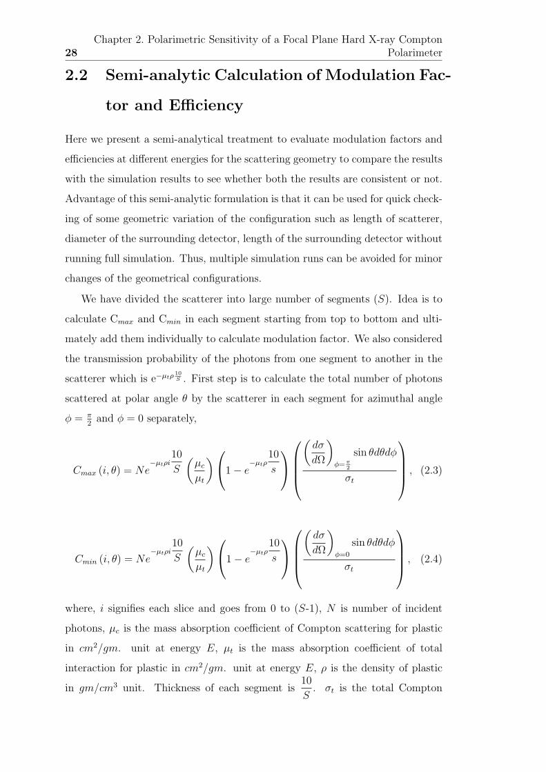
28Chapter 2. Polarimetric Sensitivity of a Focal Plane Hard X-ray Compton
Polarimeter
2.2 Semi-analytic Calculation of Modulation Fac-
tor and Efficiency
Here we present a semi-analytical treatment to evaluate modulation factors and
efficiencies at different energies for the scattering geometry to compare the results
with the simulation results to see whether both the results are consistent or not.
Advantage of this semi-analytic formulation is that it can be used for quick check-
ing of some geometric variation of the configuration such as length of scatterer,
diameter of the surrounding detector, length of the surrounding detector without
running full simulation. Thus, multiple simulation runs can be avoided for minor
changes of the geometrical configurations.
We have divided the scatterer into large number of segments (S). Idea is to
calculate Cmax and Cmin in each segment starting from top to bottom and ulti-
mately add them individually to calculate modulation factor. We also considered
the transmission probability of the photons from one segment to another in the
scatterer which is e−µtρ10S . First step is to calculate the total number of photons
scattered at polar angle θ by the scatterer in each segment for azimuthal angle
φ = π2
and φ = 0 separately,
Cmax (i, θ) = Ne−µtρi
10
S
(µc
µt
)1 − e−µtρ
10
s
(dσ
dΩ
)φ=π
2
sin θdθdφ
σt
, (2.3)
Cmin (i, θ) = Ne−µtρi
10
S
(µc
µt
)1 − e−µtρ
10
s
(dσ
dΩ
)φ=0
sin θdθdφ
σt
, (2.4)
where, i signifies each slice and goes from 0 to (S-1), N is number of incident
photons, µc is the mass absorption coefficient of Compton scattering for plastic
in cm2/gm. unit at energy E, µt is the mass absorption coefficient of total
interaction for plastic in cm2/gm. unit at energy E, ρ is the density of plastic
in gm/cm3 unit. Thickness of each segment is10
S. σt is the total Compton

2.2. Semi-analytic Calculation of Modulation Factor and Efficiency 29
scattering cross-section i.e.
σt =
∫ π
0
r202
(E
′
E0
)2 (E
′
E0
+E0
E ′ − sin2 θ
)2π sin θ dθ. (2.5)
The ratio of cross-sections (Eq. 1.8 and Eq. 2.5) gives the fraction of photons
scattered at angle θ. Since only those photons which are scattered at a partic-
ular range of angles will be absorbed by the CsI scintillators, so the next step
is to integrate the equation over the angular range covered by the surrounding
scintillators for each segment. This angle range (θmin to θmax) depends on the
geometry and energy deposition during scattering in plastic scintillator and the
segment from where scattering takes place. Here we assume 100% detection effi-
ciency of the CsI detectors. For each slice, θmin and θmax are calculated properly
(see Fig. 2.3). From the scattering geometry, we obtain
Figure 2.3: Schematic view of the scattering geometry. θmin and θmax are respec-
tively the minimum and maximum scattering angle
θmax = sin−1 x + 5√(x + 5)2 + (2.65 + 0.5)2
, (2.6)

30Chapter 2. Polarimetric Sensitivity of a Focal Plane Hard X-ray Compton
Polarimeter
θmin = sin−1 2.65 + 0.5√(10 − x)2 + (2.65 + 0.5)2
. (2.7)
For high energy photons the scattering takes place in the forward direction. The
minimum scattering angle depends on the threshold energy in the scatterer and
is equal to cos−1
(1 − Ethresmec
2
E (E − Ethres)
), where Ethres is the energy threshold in
scatterer and E is energy of the incident photons. To make sure that only those
photons scattered towards the CsI scintillators are counted, we have to take either
sine or cosine function whichever is maximum as lower limit of integration. In
the last step, the contributions from all the segments are summed over and we
get
Cmax =i=S−1∑i=0
Ne−µtρi
10
S
(µc
µt
)1 − e−µtρ
10
s
θmax∫θmin
(dσdΩ
)φ=π
2
sin θ dθ dφ
σt
,
(2.8)
Cmin =i=S−1∑i=0
Ne−µtρi
10
S
(µc
µt
)1 − e−µtρ
10
s
θmax∫θmin
(dσdΩ
)φ=0
sin θ dθ dφ
σt
.
(2.9)
Modulation factor can be obtained from Eq. 2.8 and Eq. 2.9
µ (E) =Cmax − Cmin
Cmax + Cmin
. (2.10)
Efficiency is calculated in a similar way. Assuming 100% efficiency of the
CsI detectors in the energy range of operation, we estimate the polarimetric
efficiency by calculating the total number of photons scattered by all the segments
in the plastic scatterer towards the surrounding CsI scintillators. Using the same
approach, the efficiency is determined as
ε =i=S−1∑i=0
e−µtρi
10
S
(µc
µt
)1 − e−µtρ
10
s
θmax∫θmin
(dσdΩ
)2π sin θ dθ
σt
. (2.11)

2.2. Semi-analytic Calculation of Modulation Factor and Efficiency 31
To take care of the dead spaces in between the CsI detectors a factor of 1− 32×0.022π×2.65
is multiplied with the above equation.
Results of these calculations are shown in Fig. 2.4 as continuous lines. It
Figure 2.4: Modulation factor, polarimeter efficiency and figure of merit as a func-
tion of energy. Black triangles and black solid line represent simulation and analytical
results respectively for 1 keV threshold. Red asterisks and red solid line represent the
simulation and analytical results respectively for 2 keV threshold
can be seen that the semi-analytical results for modulation factor agree well
with the simulation results for most of the energy range, though there is slight
discrepancy at lower energies. In case of efficiency, the simulated efficiency is
slightly lower than the calculated one. However, it should be noted that in this
analytic calculation, we have ignored some of the second order effects such as
the multiscattering in surrounding scintillators and the scatterer itself, escape
of photons from the CsI detectors, the absorption of scattered photons within
the Al in between the scatterer and surrounding scintillators. These factors are
not significant for modulation factor, particularly when the number of detected
photons is very large. Modulation factor will depend on the angle range mainly,
that is why we see good agreement in the results of analytical and simulation
results. However these factors are critical for efficiency calculation and as a result

32Chapter 2. Polarimetric Sensitivity of a Focal Plane Hard X-ray Compton
Polarimeter
analytical model gives slightly higher values of efficiency.
2.3 Polarimetric Sensitivity of CXPOL
Sensitivity of polarimeter (see Eq. 1.5 in Chaper 1) depends on energy integrated
modulation factor in the energy range of operation for 100% polarized beam,
exposure time, background and rate at which source photons are detected by the
instrument which in turn depends on efficiency of polarimeter, source intensity
and effective area of the mirror used to focus the X-rays. For MDP calculation
we have used the NuSTAR optics effective area [97]. NuSTAR can focus photons
from 5 keV to 80 keV. If the threshold is assumed to be 2 keV, polarimeter starts
working from 26 keV whereas for 1 keV threshold lower cut off is 18 keV. First
the average modulation factor is estimated in the working energy range (18 −
80 keV and 26 − 80 keV) which for 1 keV and 2 keV threshold is around 60.5%
and 60% respectively. This proves the excellent polarimetric performance of this
focal plane polarimeter. Source count rate is calculated as follows
Rsrc =
E2∫E1
Aeff (E) I (E) ε (E) dE, (2.12)
where Aeff (E) is the effective area of NuSTAR, I(E) is the source intensity for
Crab like spectrum, ε(E) is the polarimeter efficiency at energy E. Value of E1
depends on threshold in scatterer and E2 is 80 keV as we are considering NuSTAR
optics. We have considered 100 ks and 1 Ms exposure for sensitivity estimation.
Background calculation is discussed in detail below.
2.3.1 Spurious events calculation
Background for a focal plane Compton polarimeter is generally very small. The
only source of spurious events in Compton polarimeters is the chance coincidence
between the random background events in the scatterer and in the absorbers
within the coincidence time window. Using Poissons statistics in the coincidence

2.4. Results and Discussions 33
window one obtains the rate of spurious events due to the chance coincidence,
Nsp =(1 − e−NscattererT
)Nabsorber, (2.13)
where Nscatterer (= N1 + N2) is the sum of rate of random background events
in the scatterer (N1) and the cosmic X-ray background rate (N2) in scatterer.
Nabsorber is the rate of random instrumental background events in the absorbers.
Rate at which the cosmic X-ray photons are detected in the scatterer has been
calculated using cosmic X-ray background spectrum [98]. Since the FOV of focal
plane detector is very small, this value is very small. The cosmic X-ray photons
coming from the sky within the detector field of view may be scattered by the
scatterer and absorbed by the absorbers. This may also lead to spurious Compton
events (Nsky). Therefore the rate of total spurious events in the polarimeter can
be written as
Nsp =(1 − e−NscattererT
)Nabsorber + Nsky. (2.14)
Since the value of Nsky is very small due to narrow FOV, the random particle
events will dominate the background. Since the actual instrumental background
generally depend on the variety of factors such as spacecraft, orbit, time etc.
which cannot be estimated at present, we assumed a range of instrumental back-
ground rate from 0.5 cnt cc−1s−1 as a typical condition and 5 cnt cc−1s−1 as
extreme condition. We calculated the spurious events rates corresponding to
these two limiting instrumental background rates keeping the time coincidence
window of 10 µs , which is then used for calculating MDP values.
2.4 Results and Discussions
With the method discussed in previous section, we estimated MDP for different
Crab intensities which are shown in Fig. 2.5. We see for 100 mCrab source the
MDP is 0.9% with 3σ confidence level with 1 Ms of exposure time (black solid
lines, asterisks), which qualifies this focal plane polarimeter as a sensitive instru-
ment. However for 100 ks exposure, the sensitivity decreases to 3%. We have also
analysed the simulation data by selecting only valid/ideal Compton events and
find that the results are almost identical, which suggests that this configuration

34Chapter 2. Polarimetric Sensitivity of a Focal Plane Hard X-ray Compton
Polarimeter
Figure 2.5: MDP as a function of source intensity in Crab unit. Solid lines
represent results obtained assuming single NuSTAR mirror area. Dashed lines refer to
5 times larger NuSTAR area. 1 Ms and 100 ks exposure times are denoted by triangles
and asterisks respectively. The backgrounds considered here are 0.5 cnt cc−1s−1 (thin
lines) and 5 cnt cc−1s−1 (thick lines)
is very close to the ideal Compton polarimeter configuration. MDP values have
been calculated for random instrumental background rate of 0.5 cnt cc−1s−1 (thin
lines) and in extreme condition of 5 cnt cc−1s−1 (thick lines); however there is
not much change in MDP with background beyond 100 mCrab. In Fig. 2.5, we
have shown that sensitivity can be increased significantly using next generation
of hard X-ray focusing optics with collecting area 5 times larger than that of NuS-
TAR area (dashed lines). With this configuration, MDP for 100 mCrab source
decreases to 0.4% for 1 Ms exposure and 1.3% for 100 ks exposure. Fig. 2.5
clearly suggests that sensitivity of the polarimeter is improved for 1 keV energy
threshold in scatterer instead of 2 keV. Here, it is to be noted that reflection off
the hard X-ray mirror may introduce small artificial modulation in the azimuthal
angle distribution due to the dependence of mirror reflectance on the polarization
plane. Recent studies [99] suggest that change in polarization because of the hard
X-ray mirrors is around ∼1%, therefore limiting the sensitivity of the polarimeters

2.4. Results and Discussions 35
at the focal plane of such hard X-ray telescopes to ∼1%. Another important point
for this kind of focal plane polarimetric configuration is the strict requirement of
co-alignment of the mirror optic axis and the scatterer axis. Sight deviation of the
focal position from the scatterer axis, either permanent or temporal due to jitter,
may introduce artificial modulation in the azimuthal angle distribution. These
factors are important in optimizing the scatterer diameter for the polarimeter.
The depth of the focus along the scatterer axis should also be optimized such that
loss of photons due to leakage through the scatterer is minimized. It depends on
the convergence of radiation from the mirror and the length of the scatterer which
can be inferred by simulating the actual optics system along with the CXPOL
configuration.
In Fig. 2.6, we have shown that energy dependent polarization measurement
is possible with this focal plane polarimeter which is very useful to study the X-
ray objects. Assuming energy resolution about 10 keV FWHM, estimated MDP
Figure 2.6: MDP of the Compton Polarimeter as a function of energy. Triangle
and asterisks denote 100 mCrab and 1 Crab source intensity respectively. Red and
black stand for 2 keV and 1 keV threshold respectively in the plastic scatterer. Dashed
lines represent 5 times larger NuSTAR area. The exposure time considered here is 1
Ms and background is 0.5 cnt cc−1s−1

36Chapter 2. Polarimetric Sensitivity of a Focal Plane Hard X-ray Compton
Polarimeter
for 100 mCrab and 1 Crab have been shown in the figure (triangle and asterisks)
for 1 Ms exposure. The dashed lines correspond to the 5 times larger NuSTAR
area. The slight difference in sensitivity at lower energies for 1 keV (black) and
2 keV (red) threshold is due to higher modulation factor and efficiency for 1 keV
threshold compared to 2 keV threshold. A particular energy bin corresponds to
almost same amount of flux. As energy increases, modulation factor for 2 keV
threshold exceeds that for 1 keV threshold, however due to low efficiency the
MDP values remain almost same.
2.5 Summary
In this chapter, we described an optimized Compton polarimeter configuration
at the focal plane of NuSTAR kind of hard X-ray optics. Geant−4 simulations
suggest that we can achieve 1% MDP for 100 mCrab source with this instrument
for 1 Ms exposure. To measure polarization of the celestial X-ray sources we need
this kind of sensitivity. With the next generation of hard X-ray focussing optics,
we can achieve even better sensitivity with this kind of focal plane polarimeter.
As simulation results suggests, energy threshold in plastic scatterer is the key
parameter which will decide the sensitivity of the instrument. Therefore, it is
important to measure the threshold in plastic first and lower it down as much as
possible before integrating the whole system to investigate its overall performance.
The results of the prototype of the instrument are reported in the next chapter.

Chapter 3
Development of the Focal Plane
Compton Polarimeter
In Chapter 2, we described detailed simulation study of the expected sensitiv-
ity of our planned configuration of the focal plane Compton polarimeter, when
coupled to the NuSTAR type hard X-ray optics, assuming two different values
of low energy thresholds - 2 keV and 1 keV, for the active plastic scatterer. In
order to have better understanding of the behavior of the scatterer for very low
energy deposition, we carried out a controlled Compton scattering experiment
with the actual plastic scatterer. In this chapter, we describe the experiment
in detail and present the experimental results. The photons scattered by plas-
tic scatterer arecollected by a cylindrical array of CsI(Tl) scintillators which are
read by Si Photomultiplier (SiPM). Use of the new generation SiPMs ensures
the compactness of the instrument which is essential for the design of focal plane
detectors. After complete characterization of the plastic scatterer, we charac-
terize the CsI(Tl)-SiPM absorbers in Sec. 3.5. In Sec. 3.6, we finally present
the experimental results from the fully assembled configuration of the Compton
polarimeter.
37

38 Chapter 3. Development of the Focal Plane Compton Polarimeter
3.1 Characterization of the Plastic Scatterer
Focal plane Compton polarimeter uses long thin low-Z scatterer, typically plastic
scintillator, to maximize the Compton scattering probability. While it is possi-
ble to conceive Compton polarimeter configurations with Silicon (active detector
with second lowest atomic number), polarimetric sensitivity of such configuration
is significantly less than those using plastic scintillator as scatterer [100]. Other
organic scintillators having higher density but same effective Z as plastic scin-
tillator may be better suited for active scatterer. However, these need careful
evaluation for comparative operational advantage. Therefore, plastic scintillators
are the usual choice for dedicated hard X-ray polarimeters, when polarimetric
information is the main concern. The central scatterer is surrounded by high
Z absorbers to measure the azimuthal distribution of the scattered photons. In
all such configurations of Compton polarimeters, the lowest possible energy for
which polarization can be measured depends on the lower energy threshold of
the active scatterer. The lower energy threshold for polarization measurement is
a very important parameter for any Compton polarimeter because it determines
the lower energy limit for the polarimeter and affects overall sensitivity of the
polarimeter too. Since the number of source photons increases significantly as
energy threshold decreases, improvement of lower energy threshold by even a few
keV can greatly improve the sensitivity of the polarimeter (see Fig. 3.1).
Sensitivity of the polarimeter is generally given in terms of the Minimum
Detectable Polarization (MDP) at the confidence level of 99% [101], and is defined
as
MDP99% =4.29
Rsrc µ100
√Rsrc + Rbkg
T, (3.1)
where, µ100 is the modulation factor for 100% polarized beam. Rsrc and Rbkg are
the source and background count rate respectively. T is the exposure time. The
modulation factor, µ100, depends on the geometry of Compton polarimeter and is
typically in the range of 20% to 50%. The exposure time for the present generation
polarimetric observations is of the order of 100 ks to 1 Ms. The dependence of
MDP on the lower energy detection limit of the active scatterer comes form the
source count rate, Rsrc; lower the threshold, higher the value of Rsrc and better is

3.1. Characterization of the Plastic Scatterer 39
Figure 3.1: LogN-LogS plot obtained from Swift BAT 70 month hard X-ray sur-
vey. The vertical solid and dashed lines represent the source intinseties corresponding
to the MDP of 3% with 1 Ms exposure and MDP of 20% with 100 ks exposure respec-
tively. Different colors represent different threshold energies in the active scatterer
the sensitivity. The astrophysical significance of this dependence can be seen from
Fig. 3.1, which shows the number of X-ray sources accessible for the polarimetric
investigation for different lower energy thresholds of the active scatterer. This
figure shows the logN − logS plot based on the Swift-BAT hard X-ray catalog
resulting from 70 months observations. There are total 1171 hard X-ray sources
in the catalog, observed in 14 keV to 195 keV energy band. This logN − logS
plot is over plotted by the source intensities corresponding to the specified values
of MDP, exposure time and the lower energy threshold of the scatterer. These
source intensities are computed using Eq. 3.1 for different scatterer thresholds (1
keV, 2 keV, 3 keV, 4 keV and 5 keV) assuming Crab like spectra and convolving
the source spectra with Nustar kind of hard X-ray mirror effective area. The
modulation factor, µ100 used here is obtained from our Geant−4 simulations
reported in chapter 2. The vertical solid and dashed lines represent 3% MDP
in 1 Ms and 20% MDP in 100 ks respectively, whereas different colors represent
different scatterer thresholds. It can be seen that for lower threshold, number

40 Chapter 3. Development of the Focal Plane Compton Polarimeter
of observable sources accessible for investigation of polarization greater than a
particular MDP, is significantly larger than that for higher threshold. That is why,
it is important to know the realistic threshold energy of the primary scatterer.
However, the plastic scatterer is not expected to have a sharp energy threshold
because X-ray detection in the plastic scintillator is essentially a statistical process
and depends on various factors such as location of the interaction, light collection
efficiency etc. Therefore, such a detector is likely to have decreasing probability
of low energy depositions in the plastic being recorded. Thus for any Compton
polarimeter design, it is very important to have accurate understanding of the
behavior of the active scatterer for low energy depositions so as to have more
realistic estimate of the polarimetric sensitivity.
In this context, we carried out a Compton scattering experiment which di-
rectly probes the behavior of the active scatterer for very low energy depositions.
The experiment uses the same configuration of the plastic scintillator planed to be
used in the Compton polarimeter. Here we detect the Compton scattered X-rays
using an independent detector at different scattering angles for an X-ray beam
of known energy incident on the plastic scintillator along its axis. Recently, [102]
have reported a similar study of the active scatterer based on the same con-
cept. They concluded that the polarization measurements down to ∼20 keV are
possible by using plastic scintillator as an active scatterer. However, their exper-
imental setup was limited to a fixed geometry of the source, the scatterer and
the absorber. We carried out a similar experiment, but with an improved experi-
mental setup which allowed control over the scattering angle and thus the energy
deposited in the scatterer, to investigate the response of the plastic scintillator
at various deposited energies.
3.2 Description of the Experiment
3.2.1 Experiment setup
Typically, the lower energy threshold for an X-ray detector is measured either
by directly measuring low energy X-rays from a suitable mono-energetic X-ray

3.2. Description of the Experiment 41
source or by extrapolating the peak positions to energy relation to the noise
floor of the detector. However, these methods are not suitable for our present
objective because of two reasons - 1. energy resolution of the plastic scintillator
is very poor and hence extrapolation method can not provide accurate threshold,
and 2. the encapsulation required for the scintillator prevents transmission of the
X-rays with energies less than ∼5 keV. For typical detector applications in such
conditions, the transmission of the entrance window would determine the lower
energy threshold. In case of the plastic scintillator as scatterer for a Compton
polarimeter, the energy range of interest for incident X-rays is > 10 keV and
hence very thin entrance window of Beryllium, as is typically used to achieve
high window transmission, is not necessary. Here the energy range of interest
for detection of the deposited energy is ∼1 keV to 5 keV. Therefore we employ
the same principle of Compton scattering to investigate the response of plastic
detector to small energy deposition.
If a photon of energy E is Compton scattered at an angle θ, the energy
deposited (recoil energy of electron) is given by,
∆E = E − E
1 + Emec2
(1 − cos θ), (3.2)
where, mec2 is the electron rest mass. Fig. 3.2 shows variation of the deposited
energy in scatterer as a function of scattering angle for different energies of the
incident photon. It can be seen that the incident photons with energies of ∼20
keV to 60 keV and scattered between 30 - 150 angles, provide opportunity to
investigate the scatterer threshold in ∼0.5 keV to 10 keV.
In the actual experiment, we detect the Compton scattered X-ray photons
with energies of 59.5 keV and 22.2 keV (from radioactive sources 241Am and
109Cd respectively), in the scattering angle range of 25 - 140, simultaneously
with the trigger signal from the plastic scatterer. Fig. 3.3 shows the experi-
mental setup, which uses the plastic scatterer identical to the one which will be
used in our planned configuration of the focal plane Compton polarimeter. The
scatterer is of 5 mm diameter and 100 mm length and is surrounded by 1 mm
thick Aluminum cylinder and a 0.5 mm thick Aluminum entrance window. It was
obtained from Saint-Gobain as an integrated module containing plastic scintilla-

42 Chapter 3. Development of the Focal Plane Compton Polarimeter
Figure 3.2: Deposited energy in Compton scattering as a function of scattering
angle and photon energy. Each line corresponds to a particular incident photon energy
in keV as mentioned in the plot
tor (BC404) coupled to a photo-multiplier tube (PMT - Hamamatsu R6095 with
bialkali photocathode with maximum quantum efficiency of ∼ 25% at 420 nm).
In the polarimeter configuration, the scatterer will be surrounded by a cylindrical
array of CsI(Tl) scintillators, each of dimension 5 mm × 5 mm × 150 mm, to
measure the azimuthal distribution of the scattered photons. In the present ex-
periment, we are only interested in the polar scattering angle, and hence we use a
small CdTe detector placed on a rotating arm. We used the standard X-123CdTe
system from Amptek [103], which is kept on the rotating arm. The X-123CdTe
is a compact integrated system consisting of 1 mm thick CdTe (9 mm2 active
area), pre-amplifier, digital pulse processor, MCA, and power supply. It also has
a ‘gated’ mode of operation, in which it accepts an event only if the gate is kept
‘ON’ by applying a logic pulse. We use this mode to enforce the simultaneity
between the plastic scatterer and the CdTe detector. As shown in Fig. 3.3, the
source photons from radioactive source placed in front of the scatterer, are scat-
tered by plastic and the scattered photons are detected by the CdTe detector
kept at known angle. Positions of these two detectors can be adjusted in order to

3.2. Description of the Experiment 43
Figure 3.3: Left: Schematic view of our experiment setup. Scattered photons
from plastic are absorbed by CdTe kept at angle θ. Right: actual experiment setup -
Axes of plastic scintillator (along with PMT and CSPA), source, and CdTe are kept
at the same plane using Al blocks. CdTe is kept on a rotating arm in order to detect
photons at different scattering angles
optimize the interaction location. A collimator (70 mm long and 7 mm opening)
made of Al is used in front of CdTe window to localize the scattering region.
The collimator is wrapped by 1 mm thick lead to avoid contamination by any
unwanted events. FOV of the collimator is around 10, which allows to know
the position of the interaction in the plastic scintillator within few mm. It is
crucial to maintain the alignment of the axes of source aperture, plastic rod and
CdTe collimator to keep them in the same plane and a special care was taken to
maintain the alignment at different scattering angles. In order to maximise the
scattered counts in CdTe, a region at the top of the plastic was localised.
When an incident photon deposits sufficient amount of energy in the plastic
scintillator, either by the photoelectric interaction or Compton scattering, a logic
pulse with fixed width of 3 µs is generated by the front-end electronics. The front-
end electronics consists of a CSPA followed by a fast shaping amplifier (unipolar
type with shaping time constant of 2.6 µs) and a comparator as shown in the
block schematic in Fig. 3.4. Sensitivity of the scatterer also depends on the
HV bias for the PMT and comparator threshold. The optimum values for HV
and comparator threshold were found to be 1 kV and 50 mV respectively during
the initial trials and then were fixed for the entire experiment. The logic pulse
generated by the front-end electronics is then fed to the input of ‘Gate’ of the

44 Chapter 3. Development of the Focal Plane Compton Polarimeter
Figure 3.4: Block schematic for the coincidence unit between plastic scintillator
and X123CdTe
X123CdTe system and thus it detects the photons only for the duration of 3 µs
following a trigger from the plastic scatterer. For each scattering angle, we acquire
two sets of spectra from CdTe - first, with the coincidence between CdTe and
plastic enforced, which actually gives the Compton scattering events and second,
without coincidence (PMT HV off), i.e. plastic behaving as a passive scatterer.
With the simultaneity between plastic and CdTe enforced, it is expected that
only a very small fraction of all the triggers would have simultaneous detection in
the CdTe and hence total experiment duration has to be very large (few hours)
but would result in relatively very short acquisition time of few minutes. This
has important implication in our semi-analytical modeling as discussed in the
following sections.
3.2.2 Results
The spectra acquired from the CdTe detector at three different scattering angles
in both the modes i.e. in coincidence with the scatterer and without coincidence,
for both 59.5 keV (from 241Am) and 22.2 keV (from 109Cd) incident X-rays are
shown in Fig. 3.5. These spectra are normalized with respect to actual acquisition
time (time for which CdTe ‘Gate’ was on during the exposure). In each plot, the

3.2. Description of the Experiment 45
solid line represents spectrum in coincidence mode and the dashed line represents
spectrum in non-coincidence mode. The backgrounds in both coincidence and
non-coincidence mode are negligible compared to the respective source counts. It
can be seen that the count rate in the coincidence mode is higher than that in
the non-coincidence mode as expected, because in coincidence mode, the CdTe
detector accepts an event only for a short duration after each trigger in the plastic
scatterer. The energy of the Compton peaks also changes with scattering angle
as expected. The detection of Compton peak at 60 from 22.2 keV X-rays clearly
shows that the plastic scatterer can detect energy depositions less than 1 keV. Fig.
Figure 3.5: Coincidence (solid) and non-coincidence (dashed) spectra observed
with the CdTe detector at different scattering angles. Upper panel (left to right) shows
spectra for 59.5 keV from 241Am at scattering angles 140, 90, 35 respectively. Lower
panel (left to right) shows spectra for 22.2 keV of 109Cd at scattering angles 140, 90,
60 respectively. Energy of primary incident photons have been represented by the
dotted lines
3.6 shows the observed count rate at all measured angles for both the sources.
Total counts for the 241Am are obtained by summing over ±3 FWHM from the
peak energy for each spectrum, however for the 109Cd, total counts are obtained
by summing over -3 FWHM to +1 FWHM in order to avoid contribution from

46 Chapter 3. Development of the Focal Plane Compton Polarimeter
the secondary peak at 25 keV. Again, for each spectrum the count rate is with
respect to the actual acquisition time which is related to the exposure time by
equation
Tco = T expco TwinRtrig, (3.3)
where, Tco (∼200 sec for 241Am and ∼100 sec for 109Cd) and T expco (∼2 hrs for
241Am and ∼7 hrs for 109Cd) are acquisition time and exposure time respectively
in coincidence condition, Rtrig is trigger rate in plastic and Twin is the coincidence
time window (∼3 µs). The acquisition time is measured by the CdTe detector,
which allows to calculate trigger rate for each measurement.
The count rates in coincidence mode, Rco, and in non-coincidence mode, Rnco,
are given by
Rco =Nco
Tco
, (3.4)
Rnco =Nnco
Tnco
, (3.5)
where Nco and Nnco are the summed counts under these peaks (Compton and
Rayleigh) in coincidence and non-coincidence mode respectively for a particular
angular position θ of CdTe. Tnco (0.5 hours for 241Am and 1.5 hours for 109Cd)
is the acquisition time in non-coincidence mode.
Since, Tco Tnco, Rco Rnco as can be seen in the figure with open circles
and filled circles representing coincidence and non-coincidence modes respectively.
At lower angles (< 45), there is also a finite probability of the source photons
directly entering into the CdTe detector, which leads to increase in count rate
in both non-coincidence and coincidence mode due to the chance coincidences.
This problem is only present for 241Am source, because in case of 109Cd, the
measurements are limited to scattering up to 60. To correct for the spurious
count rate due to direct exposure, we measured number of counts at lower an-
gles for 241Am without having the plastic scintillator in place. This configuration
then measures any ‘leakage’ of photons through the intervening material. How-
ever, direct subtraction of these counts from the observed counts for 241Am at
the respective lower angles would underestimate the non-coincidence count rate,
because the plastic scintillator and the surrounding Aluminum may absorb some

3.2. Description of the Experiment 47
of these photons. We estimated this absorption fraction for different angles at
energy 59.54 keV based on the geometry of our experiment setup. The observed
count rate due to direct exposure (without the plastic scatterer) is then corrected
by this absorption fraction and then subtracted from the observed count rate
(with the plastic scatterer) to calculate correct count rate due to scattering only.
The error bars shown here combine both statistical and systematic uncertain-
ties. The sources of systematics are misalignment between collimator and plastic
scatterer, uncertainty in angle measurement, uncertainty in the center of rotation
of CdTe around plastic and the uncertainty in the coincidence time window. The
most prominent source of error is the misalignment of plastic and the collimator,
for which we have tried to control within the experimental limits. The contri-
butions of each of these sources to overall systematic error is estimated as per
following discussion. Error due to misalignment between plastic axis and CdTe
collimator axis is obtained by geometrically estimating the intersection area of
CdTe field of view with the plastic for a given angle. A misalignment of 1 mm
introduces a minimum of 9% error across all the angles, contribution is maximum
(∼14%) for angles close to 90 and minimum for lower scattering angles (∼9%).
Error due to uncertainty in angle measurement is computed by estimating the
change in Compton and Rayleigh scattering cross-section and is found to be less
than 0.1% at angles close to 90 and about 1% at other angles for an angle mea-
surement uncertainty of 1. Error due to uncertainty in coincidence time window
is directly proportional to the amount of uncertainty present and its value is
found to be 6% for uncertainty of 0.2 µs. Uncertainty in the central position of
interaction reflects change in transmission probability of photons. Contribution
of this is found to be of the order of 2% for 59.54 keV and 4% for 22.2 keV.
Systematic errors are therefore angle dependent. We estimated combined sys-
tematic uncertainties to be 10% at lower and higher scattering angles and 16%
at angles close to 90. These are added to the statistical uncertainties in quadra-
ture. Each measurement has been repeated several times to have confidence in
the observed count rates and we have considered an average count rates from
multiple measurements where necessary.

48 Chapter 3. Development of the Focal Plane Compton Polarimeter
Figure 3.6: Observed count rate for 59.5 keV (left) and 22.2 keV (right) for
coincidence (open circles) and non-coincidence (filled circles) modes as a function of
scattering angles
Fig. 3.6 shows that, at higher angles the coincidence count rate is more
than that in the non-coincidence count rate because of large energy deposition,
which is above the threshold. As we move towards the lower scattering angles,
because of lower energy deposition, fraction of valid Compton scattered photons
decreases and consequently the coincidence and non-coincidence count rates tend
to match each other. Thus this figure demonstrates the essence of our experiment
in qualitative terms, that though the plastic scatterer is able to detect energy
deposition as low as ∼1 keV, the efficiency of detection decreases gradually with
decreasing energy.
However, these representations of count rate vs. scattering angles are not suit-
able for quantitative estimation of detection efficiency as a function of deposited
energy in the scatterer because of the fact that the trigger rate in the plastic
scatterer is not constant across all the scattering angles. In order to minimize
the total exposure times, particularly in the coincidence mode, it is necessary to
keep the source as close as possible from the scatterer. However, this distance is
different for different scattering angles, which results in variation of the total trig-
ger rate (i.e. total interactions including photoelectric and detectable Compton
scattering interactions) in the plastic scatterer.
Therefore it is necessary to normalize count rates with respect to the number
of triggers in plastic. If Rtrig is the trigger rate in plastic for angle θ (obtained
from Eq. 3.3), then normalized count rates, i.e. the number counts in the CdTe

3.2. Description of the Experiment 49
Figure 3.7: Normalised count rate with respect to the total number of triggers
in plastic (see text for further details) for 59.5 keV (left) and 22.2 keV (right) as a
function of scattering angles. Open and filled circles stand for coincidence and non-
coincidence modes respectively.
detector per trigger in the plastic scatterer, at θ are given by
Rnormco =
Nco
T expco Rtrig
, (3.6)
Rnormnco =
Nnco
T expncoRtrig
. (3.7)
Denominator in Eq. 3.6 and Eq. 3.7 is total number of triggers in plastic during
the experiment. Fig. 3.7 shows the normalized rates in coincidence and non-
coincidence modes for both the sources. Since, T expco T exp
nco , the normalized
rate in non-coincidence mode, represented by filled circles, is much higher than
that in the coincidence mode, denoted by open circles. Since, statistical error
on count rate is inversely proportional to exposure time, error in non-coincidence
mode is larger too. We see that count rate in coincidence mode is decreasing
in a steady manner. This clearly shows that the plastic scatterer does not have
a sharp detection threshold, rather the detection efficiency gradually decreases
with decreasing deposited energy.
It can be seen that the normalized count rate in non-coincidence mode is
always greater than that in coincidence mode. For 241Am, X-rays scattered at
large scattering angles, the energy deposited in the scatterer is more than ∼5 keV,
which is always expected to generate a trigger in the scatterer. Thus it is expected
that in this range the normalized rate in both non-coincidence and coincidence

50 Chapter 3. Development of the Focal Plane Compton Polarimeter
mode should be same, because of much smaller probability of the Rayleigh scat-
tering at this energy. However, the fact that the observed normalized count rate
in non-coincidence mode is higher than that in coincidence mode, suggests that
the scattering events taking place in the material apart from the plastic scintilla-
tor, e.g. the surrounding Aluminum cylinder, because of the diverging beam, also
contribute to the non-coincidence count rate. In coincidence mode, these events
get suppressed due to the requirement of the simultaneity. This further suggests
that the contribution of such events must be taken into account while estimating
the number of chance coincidence events in the coincidence mode as well.
3.3 Numerical Modeling
Fig. 3.7 present the number of scattered photons detected by the CdTe detector
at a given scattering angle for each trigger registered in the plastic scatterer.
Since the scattering geometry of our experiment is fairly simple, in principle
it should be possible to estimate this count rate using the knowledge of the
Compton scattering cross-section of the plastic scatterer. However, we find that
such simple minded calculation does not give count rate estimation, or the trend
of its variation with scattering angle, which can be directly compared with the
observed results. On further investigation, we find that it is essential to consider
various factors such as -
• the finite scattering length as viewed by the CdTe detector through colli-
mator,
• absorption of the incident photons by the entrance window in front of the
plastic scatterer,
• absorption of the photons scattered from the plastic scatterer in the sur-
rounding Aluminum,
• scattering of incident photons form the surrounding Aluminum itself,
• multiple-scattering within plastic and Al,

3.3. Numerical Modeling 51
Figure 3.8: Left: Geometric representation of the experimental setup. In the
model, total length of the plastic scatterer observed by the CdTe detector is calculated
based on this geometry, which is then further divided into a large number of small
segments as shown by the grey parallel lines. Right: Front surface of the plastic (5
mm diameter). Plastic is surrounded by 1 mm thick Al. Al surface facing the CdTe
is named as front Al and opposite surface is back Al
• efficiency of CdTe at the scattered energies,
• scattering of photons from inner Aluminium surface of collimator etc.
We attempted to model the observed results including most of these factors.
We start with Klein Nishina cross-section [52] for Compton scattering
dσKN
dΩ=
r202
(E ′
E
)2[E ′
E+
E
E ′ − sin2 θ
], (3.8)
where, E and E ′ are energies of incident and scattered photon respectively for
scattering angle θ. From Eq. 3.8, one can obtain Thomson scattering cross section
by substituting E = E ′
dσT
dΩ=
r202
[1 + cos2 θ
]. (3.9)
Here we assume that the photons from source are being scattered by plastic along
its axis. For a given angle θ, range in angle of scattering and the scattering length
are calculated from the known geometry (see Fig. 3.8).
Then we divide the scattering length into a large number of small segments
and for each segment, both polar and azimuthal scattering ranges i.e. θmin,i,
θmax,i and φmin,i, φmax,i subtended by the CdTe detector at the center of the
ith segment, are calculated. Cross-section of each segment for a photon to be
scattered in the direction of the CdTe detector, is then estimated by integrating

52 Chapter 3. Development of the Focal Plane Compton Polarimeter
Eq. 3.8 and Eq. 3.9 over these angle ranges,
σC(θ, i) =
∫ θmax,i
θmin,i
∫ φmax,i
φmin,i
dσKN
dΩsin θ dθ dφ, (3.10)
σR(θ, i) =
∫ θmax,i
θmin,i
∫ φmax,i
φmin,i
dσT
dΩsin θ dθ dφ. (3.11)
For integration over φ for ith segment, we estimated φmin and φmax at both θmin
position and θmax position and took average of φmin and average of φmax as limit
of integration.
One important point to be noted here is the cross-sections in Eq. 3.8 and Eq.
3.9 are valid for scattering off free electrons. However, in case of realistic mat-
ters, the binding effect of electrons and their momentum distributions inside the
atom introduces significant difference in the scattering distribution specially at
the lower angles. Thus the numerical values obtained from Eq. 3.10 and Eq. 3.11
are expected to differ from the actual true values because of these effects. This
point is specifically discussed in [104]. Though in our experiment forward scatter-
ing is not dominant, we accounted for these effects by considering more realistic
scattering cross-sections by including atomic form factors and incoherent scatter-
ing functions into the calculations for the scattering atom under consideration as
shown below,
σC(θ, i) =
∫ θmax,i
θmin,i
∫ φmax,i
φmin,i
dσKN
dΩS(x, Z) sin θ dθ dφ, (3.12)
σR(θ, i) =
∫ θmax,i
θmin,i
∫ φmax,i
φmin,i
dσT
dΩ|F (x, Z)|2 sin θ dθ dφ. (3.13)
where,
x = (E/hc) sin(θ/2) (3.14)
S(x, Z) and F (x, Z) are the incoherent scattering functions and atomic form
factors respectively for element of atomic number Z. The values of S(x, Z) and
F (x, Z) as a function of x are obtained from [105]. For a given incident photon
energy (E), it is possible to get these values as a function of scattering angle which
typically ranges from 0 to 160. For our purpose, we interpolated the form factor
and scattering functions at each degree and used them in Eq. 3.12 and Eq. 3.13.

3.3. Numerical Modeling 53
Since plastic is a compound material consisting of H and C atoms, form factors
and scattering functions for plastic have been computed by taking proper weight
factors into their individual form factors and scattering functions.
Dividing Eq. 3.12 and Eq. 3.13 by total Compton and Rayleigh cross-section
for ith section respectively, we get the probability of photons scattered by ith
segment reaching the CdTe detector, kept at angle θ,
PC(θ, i) =σC(θ, i)
σC,tot(i), (3.15)
PR(θ, i) =σR(θ, i)
σR,tot(i), (3.16)
where PC(θ, i) and PR(θ, i) are the fraction of total scattered photons by the ith
segment that reach CdTe. Total cross-sections have also been computed in a
similar fashion by taking into account form factors and scattering functions.
To get the total number of Compton and Rayleigh scattered photons reaching
the CdTe detector, it is necessary to multiply PC(θ, i) and PR(θ, i) by the prob-
ability of respective interaction taking place in the ith segment. This probability
is calculated using the mass attenuation co-efficients of Compton and Rayleigh
scattering for the plastic scintillator obtained from the NIST data base [106].
If ith segment has thickness ‘Sp’ (‘p’ stands for plastic), then the fraction of
photons Compton scattered by that segment is µpc
µpt[1 − e−µp
t ρpsp ] and fraction of
photons Rayleigh scattered is µpr
µpt[1 − e−µp
t ρpsp ]. Here, µpc , µ
pr, µ
pt are respectively
the Compton, Rayleigh scattering attenuation coefficient and total attenuation
coefficient of plastic at the incident photon energy, E. ρp is the density of plastic.
Therefore, fraction of incident photons detected by CdTe at angle θ is given by
Npnco(θ)
Np0
= e−µwρwtw
N−1∑i=0
e−iµpt ρpSp
µpc
µpt
(1 − e−µpt ρpSp)PC(θ, i)
+ e−µwρwtw
N−1∑i=0
e−iµpt ρpSp
µpr
µpt
(1 − e−µpt ρpSp)PR(θ, i). (3.17)
Summation is performed over all the segments (each of thickness ‘Sp’) in plastic.
N is total number of segments. Np0 refers to photons incident on plastic. The
exponential term, e−µwρwtw , takes into account the transmission through a thin

54 Chapter 3. Development of the Focal Plane Compton Polarimeter
window made of plastic (thickness, tw = 3 mm; density, ρw; total absorption co-
efficient at E, µw) at the front of plastic scintillator. The first and second part
in Eq. 3.17 stands for Compton and Rayleigh events in plastic respectively. We
have assumed 100% detection efficiency of CdTe which is a good approximation,
as for 1 mm CdTe efficiency falls from 100% beyond 60 keV.
A fraction of these scattered photons will be absorbed by the surrounding
front Al (see Fig. 3.8) of thickness 1 mm. However, the photon path length
(absorption thickness) depends on scattering angle. Absorption coefficient of Al
also depends on the scattered energy. Hence both these factors will vary from
segment to segment. For simplicity in calculation, we estimated the photon path
length corresponding to the mean of minimum and maximum scattering angle for
each segment. Absorption co-efficient is also evaluated at energy corresponding to
that mean scattering angle. The angle range being very small, this approximation
holds good. If tfa and µfat,E′ (E ′ is the scattered energy corresponding to mean
scattering angle) are the absorption thickness and total absorption co-efficient of
front Al for ith segment, then absorption factor is given by e−µfa
t,E′ρatfa
, where ρa
is the density of Al and ‘fa’ stands for front Al. With the inclusion of this factor,
Eq. 3.17 is modified to
Npnco(θ)
Np0
=Np,C
nco (θ)
Np0
+Np,R
nco (θ)
Np0
, (3.18)
where, first (Compton) and second term (Rayleigh) are given by
Np,Cnco (θ)
Np0
= e−µwρwtw
N−1∑i=0
e−iµpt ρpSp
µpc
µpt
(1 − e−µpt ρpSp)PC(θ, i) e
−µfa
t,E′ρatfa
, (3.19)
Np,Rnco (θ)
Np0
= e−µwρwtw
N−1∑i=0
e−iµpt ρpSp
µpr
µpt
(1 − e−µpt ρpSp)PR(θ, i) e−µfa
t,Eρatfa . (3.20)
It is to be noted here that the attenuation coefficients of Aluminum needs to
be taken at respective energies of the photon i.e. for Compton scattering it is the
energy of the scattered photon and for Rayleigh scattering it is the energy of the
incident photon.
As discussed earlier, it is essential to consider scattering from the Aluminum
cylinder surrounding the plastic scatterer. Keeping the source opening and

3.3. Numerical Modeling 55
source-plastic distance in mind, it is assumed that radiation is uniform over the
plastic and surrounding Al. We estimated the contribution in scattered photons
from both front Al and back Al (see Fig. 3.8) with the same approach mentioned
above. It is assumed that the photons are scattered along the axes of front and
back Al and the angles of scattering have been calculated with respect to these
axes. Therefore, the scattering angle range for any segment is different for differ-
ent scatterers i.e. plastic, front Al and back Al. Fraction of photons scattered by
front and back Al at angle θ is given by
N fanco(θ)
N fa0
= e−µwρwtw
N−1∑i=0
e−iµat ρaSfa
µac
µat
(1 − e−µat ρaSfa)PC(θ, i)
+ e−µwρwtw
N−1∑i=0
e−iµat ρaSfa
µar
µat
(1 − e−µat ρaSfa)PR(θ, i), (3.21)
N banco(θ)
N ba0
= e−µwρwtw
N−1∑i=0
e−iµat ρaSba
µac
µat
(1 − e−µat ρaSba)PC(θ, i) e
−µfa
t,E′ρatfa
e−µp
t,E′ρptp
+ e−µwρwtw
N−1∑i=0
e−iµat ρaSba
µar
µat
(1 − e−µat ρaSba)PR(θ, i) e−µfa
t,Eρatfa e−µpt,Eρptp , (3.22)
where, N fa0 and N ba
0 are the incident photons on front Al and back Al respectively.
Other symbols have their meaning as described earlier. It is to be noted that in
Eq. 3.21, the absorption terms have been dropped because there are no source of
absorption for photons scattered from front Al. However, the photons scattered
from back Al will suffer absorption from the 5 mm plastic and the 1 mm front
Al. These factors have been included in Eq. 3.22.
Now assuming uniform exposure of the incident X-rays over the plastic scat-
terer and surrounding Aluminum, it can be shown that if Np0 is the number of
photons incident on plastic, then number of photons incident on front and back
Al are respectively 2450Np
0 and 2450Np
0 (diameter of plastic is 5 mm and diameter
of plastic plus Al is 7 mm). Therefore, using Eq. 3.18, Eq. 3.21 and Eq. 3.22,
one can obtain ratio of photons scattered into CdTe at angle θ to the number of
photons incident on plastic as
Nnco(θ)
Np0
=Np
nco(θ)
Np0
+24
50
N fanco(θ)
N fa0
+24
50
N banco(θ)
N ba0
. (3.23)

56 Chapter 3. Development of the Focal Plane Compton Polarimeter
Now, the normalized count rate shown in Fig. 3.7, and as defined in Eq. 3.7,
is the ratio of number of scattered photons detected by the CdTe detector to the
total number of triggers in the plastic scatterer. Whereas the Eq. 3.23 gives the
ratio of number of scattered photons likely to be detected by the CdTe detector to
the total number of incident photons on plastic of the given energy, i.e. either 59.5
keV or 22.2 keV. These two ratios can not be compared directly because of the fact
that both 241Am and 109Cd source emit photons of multiple energies and thus all
triggers generated by the plastic scatterer included those generated by incident
photons having energies other than that of interest. Here again it is possible
to modify the ratio given by Eq. 3.23 based on the knowledge of the relative
intensities of different lines emitted by both sources. However, exact values of
relative intensities of the X-ray lines capable of generating triggers in the plastic
scatterer are not available for the sources we have used during the experiment.
Also, exact calculation of this ratio would require assumption of 100% trigger
generation efficiency at all energies. Therefore, instead of calculating the ratio of
incident photons to the triggers in the plastic scatterer, we modify Eq. 3.23 to
include a fit parameter, α, representing this ratio. This parameter also takes into
account any small deviation from the strict alignments of source to scatterer and
scatterer to CdTe axis as assumed in the model, provided that the deviation is
constant across all angles. Thus the final expression of the model is given by
Nnco(θ)
Ntrig
=Np
nco(θ)
αNp0
+24
50
N fanco(θ)
αN fa0
+24
50
N banco(θ)
αN ba0
. (3.24)
Thus to quantitatively compare the observed results with expected values, we
fit Eq. 3.24 to the results shown in Fig. 3.7 and obtain best fit value of the
parameter, α, by χ2 minimization.
3.4 Modeling Results and Discussions
Fig. 3.9 shows the fitted model (thick solid line, Eq. 3.24) with the experimental
results. For 241Am, the best fit value for parameter α is 3.65, whereas for 109Cd,
it is 0.88. These values are reasonably close to the values expected from the
available data for relative intensities of different X-ray lines for both 241Am and

3.4. Modeling Results and Discussions 57
Figure 3.9: Observed count rate in the non-coincidence mode fitted by the model.
Left plot corresponds to 59.5 keV and right plot corresponds to 22.2 keV photons.
The thick solid line represents final model (Eq. 3.24) whereas the thin lines represents
different components of the model - dashed lines: Compton scattering events from
plastic; dotted lines: Rayleigh scattering events from plastic; solid lines: sum of
Compton and Rayleigh events from plastic; dashed dot dot: scattering events from
front Al; long dashed: scattering events from back Al. Best fit values of the parameter
of the fitted curve are 3.65 and 0.88 for 59.5 keV and 22.2 keV respectively
109Cd source. Different components of the model are shown in Fig. 3.9: Compton
scattering events from plastic (dashed, Eq. 3.19), Rayleigh scattering events from
plastic (dotted, Eq. 3.20), combined Compton and Rayleigh events from plastic
(thin solid, 1st term of Eq. 3.24), scattering events (Compton + Rayleigh) from
front Al (dashed dot dot, 2nd term of Eq. 3.24) and back Al (long dashed, 3rd
term of Eq. 3.24) surrounding the plastic.
This model so far is aimed at reproducing the observed count rate in the
non-coincidence mode i.e. the scatterer is considered to be passive. The observed
count rate in the coincidence mode can be estimated from Eq. 3.19 along with the
chance coincidence rate due to all other terms i.e. Rayleigh scattering in plastic
scatterer (Eq. 3.20), scattering from the Aluminum cylinder (2nd and 3rd terms
of Eq. 3.24) as well as chance coincidence of the real Compton scattering events
which failed to generate trigger. The chance coincidence fraction of these terms
can be given by the product of trigger rate in plastic scatterer and the width of
the coincidence window i.e.,
fch = TwinRtrig, (3.25)

58 Chapter 3. Development of the Focal Plane Compton Polarimeter
Figure 3.10: Comparison between experimentally obtained coincidence count
rate and modelled count rate assuming 100% detection probability of plastic. Left
plot shows the comparison for 59.5 keV. Right plot shows the comparison for 22.2 keV
where, fch is the chance coincidence factor. Thus the total expected count rate
in the coincidence mode can be expressed as
Rnormco (θ) =
Np,Cnco (θ)
αNp0
P (E) +Np,R
nco (θ)
αNp0
fch +24
50
N fanco(θ)
αN fa0
fch
+24
50
N banco(θ)
αN ba0
fch +
(Np,C
nco (θ)
αNp0
− Np,Cnco (θ)
αNp0
P (E)
)fch, (3.26)
where, α is the best fit parameter obtained from fitting the non-coincidence mode
data. The Compton scattering term is multiplied by the energy dependent prob-
ability of generating trigger in the plastic scatterer for given energy deposition.
All the terms in this equation, except the detection probability P (E), can be
estimated using Eq. 3.6, Eq. 3.18, Eq. 3.21 and Eq. 3.22. Comparison of the
expected count rate from Eq. 3.26, assuming the detection probability to 100%,
with the observed count rate in the coincidence mode is shown in Fig. 3.10. We
see that at higher scattering angles for 241Am, modelled and experimental coinci-
dence count rate agrees well with each other implying 100% detection probability
at those energies. At lower angles for both the sources, experimental values are
significantly less than the model values indicating lower detection probability at
lower energies. This probability can be determined directly by comparing model
values with the observed values and are shown in Fig. 3.11 for both 241Am (rep-
resented by open triangles) and 109Cd (represented by filled triangles) sources.
Here the X-axes are converted from the scattering angles into the deposited ener-

3.4. Modeling Results and Discussions 59
Figure 3.11: Detection Probability of plastic scintillator as function of deposited
energy in plastic. Left: probability of event detection obtained 59.5 keV photons.
Right: Detection probability estimated from 22.2 keV.
gies corresponding to scattering of incident photons (59.5 keV and 22.2 keV) at
those angles. Fig. 3.12 shows combined data from both the sources as uniformly
increasing trigger generation efficiency of the plastic scatterer in the energy range
of 0.4 keV to 10 keV. It can be seen that there is common energy range of 0.65
keV to 1.55 keV, in the energy depositions by both the sources, corresponding to
small angle of scattering of 59.5 keV photons and large angle scattering of 22.2
keV photons, and the observed values for both the sources agree well with each
other. The small angle scattering of 22.2 keV photons gives ∼6% detection effi-
ciency at energies down to ∼0.5 keV, which then increases almost linearly up to
3.0 keV. At energies greater then 7 keV, the detection efficiency almost saturates
at 100%, as expected. The observed variation of detection efficiency can be fitted
by an empirical polynomial given in Eq. 3.27,
P (E) = 0.028E3 − 1.654E2 + 24.218E − 5.5633 . (3.27)
It is important to note few points regarding our modeling - 1) This expres-
sion for the variation of detection efficiency as a function of energy depends
on other experimental factors such as HV bias for the PMT and comparator
threshold of the front-end electronics as well as the specific configuration of the
plastic scatterer and its encapsulation. However, our modeling does not depend
on these factors as the model fitting is with respect to the observations in the
non-coincidence mode. Thus any further optimization of the experimental factors

60 Chapter 3. Development of the Focal Plane Compton Polarimeter
Figure 3.12: Detection probability as a function of deposited energy from 0.4 keV
to 10 keV. Filled and open triangles correspond to 22.2 keV and 59.5 keV photons
respectively. These data points have been fitted with an empirical polynomial shown
by solid line.
would only influence the observed count rate in coincidence mode and thus would
automatically result in better detection efficiency from the same model. 2) This
expression represents the worst case scenario in terms of the interaction position
within the plastic scatterer because in our present experiment, only the inter-
actions within top couple of centimeters of the plastic scatterer are considered.
For deeper interactions, the trigger generation efficiency may be slightly better
due to reduced light path but surely not worse than the present case. 3) This
empirical expression is valid for our configuration of the plastic scatterer (e.g. 10
cm long and 5 mm diameter BC404). For any other configuration, though the
general trend is expected to be same, the exact expression needs to be measured
separately. It is to be noted that our results agree well with the results reported
in [102] particularly for higher energy depositions. At lower energies, detection
probability for our plastic configuration is slightly less which could be because
of the fact that they used a smaller scatterer (3 cm) with scattering material
of higher light yield compared to BC404. On the other hand, detection prob-

3.4. Modeling Results and Discussions 61
abilities of the plastic scatterer in X-Calibur/PolSTAR as reported in [76] are
systematcally less compared to our results which is expected as the plastic in
X-Calibur/PolSTAR is comparatively longer around 14 cm.
Now that we have an empirical expression representing the detection efficiency
for our configuration of the plastic scatterer, we can use that to estimate the sensi-
tivity of the Compton polarimeter more accurately. In Chapter 2, we investigated
the sensitivity of a hard X-ray focal plane Compton polarimeter comprising the
same configuration of the plastic scatterer and coupled to the NuSTAR type of
hard X-ray optics. The MDP of this configuration of polarimeter was found to
be 0.9% in 1 Ms for 100 mCrab source, when the threshold for the scatterer was
assumed to be 1 keV. The MDP for threshold of 2 keV was found to be 1.2% for
the same conditions. We reanalyzed the data from the same simulations using
the above expression for energy dependent detection efficiency (see Eq. 3.27)
of the plastic scatterer and the results are shown in Fig. 3.13. It can be seen
that the MDP for the same conditions (1 Ms exposure for 100 mCrab source)
is 1.2%, indicating slightly degraded but more realistic sensitivity. The lower
energy limit for polarization measurement is also improved to ∼14 keV because
of finite probability of detecting energy depositions as low as ∼0.5 keV by the
plastic scatterer. However, it should be noted that at energies less than ∼20
keV, the properties of the material between the scatterer and the absorber, in
our case 1 mm and 0.5 mm Aluminum surrounding scatterer and in front of the
absorber respectively, become very important as the scattered photon has to pass
through it without undergoing any further interaction. We attempted to replace
the Aluminum by lower-Z materials in our simulations, but the results were not
very encouraging because of the enhanced scattering in the intervening low-Z
material, which degraded overall modulation pattern of the scattered photons.
Thus we find that, in order to improve the sensitivity as well as overall efficiency
of the Compton polarimeter, apart from the obvious optimization of the plastic
scatterer configuration and associated electronics, it is equally important that the
material between the scatterer and the absorbers has higher atomic number to
reduce scattering, and is as thin and uniform as possible to enhance transmission

62 Chapter 3. Development of the Focal Plane Compton Polarimeter
Figure 3.13: MDP as a function of source intensity. Triangles and asterisks stand
for 1 Ms and 100 ks exposure respectively. Solid lines refer to single NuSTAR collecting
area of mirror. Dashed lines refer to five times NuSTAR mirror area. Different
background rates have been denoted by thick and thin lines. For bright sources, MDP
is below 1%. However, it is to be noted that eventual polarization sensitivity will be
limited by systematics of the instrument.
of the photon scattered from the central scatterer. Overall, we find that polar-
ization measurements down to ∼15 keV are certainly possible using Compton
polarimeter. Since many celestial sources are expected to have energy dependent
X-ray polarization signatures, it is important to take into account the detection
efficiencies of the active scatterer specially at the lower energies while interpreting
the eventual energy integrated polarization measurements.
3.5 Characterization of CsI(Tl) Scintillators
In Chapter 2, we described simulation analysis of the Compton polarimeter as-
suming 32 CsI scintillators in cylindrical array. In the final experimental con-
figuration of the Compton polarimeter, the scattered photons from the plastic
scatterer are collected by 16 CsI(Tl) scintillators as shown in Fig. 3.14). Each of

3.5. Characterization of CsI(Tl) Scintillators 63
Figure 3.14: Planned Compton polarimeter configuration. The photons scattered
by the central plastic scatterer (10 cm long with 5 mm diameter) are collected by a
cylindrical array of 16 CsI(Tl) scintillators (each 15 cm long and 5 mm × 5 mm cross-
section). In Chapter 2, we showed simulation for the Compton polarimeter geometry
assuming 32 absorbers; however in the current experimental configuration, 16 CsI(Tl)
scintillators have been used
the CsI(Tl) crystal is 15 cm long and 5 mm × 5 mm cross-section (see Fig. 3.15),
procured from Saint-Gobain. The CsI(Tl) crystals are known to have high light
yield, however, for our initial experiment these crystals are selected primarily
because of their less hygroscopic nature compared to other well known inorganic
scintillators such as NaI(Tl) or LaBr3(Ce), which makes them easier to handle
in the laboratory. One important drawback of CsI(Tl) scintillator is the long
scintillation decay time, which is particularly severe in the context of readout by
SiPM. Thus our results with CsI(Tl) readout by SiPM are expected to be worst
case scenario and could be significantly improved with faster scintillators.
Each of the CsI(Tl) crystals are kept inside an aluminium case which encloses
the crystal from all sides except the side facing the scatterer and the lower end for
readout. The aluminium case is 5 mm thick on the back and 1 mm thick on the
both sides. Each of the scintillators is read by a single Si photomultiplier (SiPM)
at one end of the CsI(Tl). SiPM is a multi-pixel semiconductor photodiode system

64 Chapter 3. Development of the Focal Plane Compton Polarimeter
Figure 3.15: (a) A CsI(Tl) scintillator (5 mm × 5 mm × 150 mm) and its
aluminium holder. (b) A Si photomultiplier (3 mm × 3 mm) with its aluminium
case. (c) The complete CsI(Tl)-SiPM package. The CsI(Tl) is coupled to the SiPM
using optical glue and wrapped by a thin aluminium foil for light tightness. 16 such
CsI(Tl)-SiPM systems have been used in the final Compton polarimeter configuration
with pixels on a common Si substrate. SiPM work in Geiger mode (bias voltage
> breakdown voltage), which provides high gain (∼106) making it sensitive even
for single photon detection. The details of working principle of SiPM and other
properties can be found in [107–109].
We used SiPM procured from KETEK, Germany (SiPM PM3350), with active
area of 3 mm × 3 mm (see Fig. 3.15). The device is small, light, and robust with
low operation voltage (∼31 V) and therefore easier to handle and provides the
compactness necessary for focal plane detectors. The wide spectral range from
300 nm to 800 nm (peak wavelength 420 nm) nicely matches with the CsI(Tl)
emission spectra. There are 3600 micro-pixels (each of 50 µm × 50 µm) in a single
device. An incident photon on any micro-pixel triggers an avalanche. In low light
conditions, the number of fired micro-pixels is directly proportional to the number
of photons incident on entire active surface. Hence in such conditions the SiPM
can be used to measure the intensity of incident light by adding the signals from
all the fired micro-pixels, though individual micro-pixels are operating in Geiger
mode. One major problem with SiPM is the constant leakage current resulting
from the random firing of micro-pixles due to thermal and field excitations inside
Si, which makes it difficult for lower energy applications. At energies beyond

3.5. Characterization of CsI(Tl) Scintillators 65
100 keV, SiPM device has been proved to be a much better readout option for
scintillators than conventional vacuum PMTs [110, 111]. Here we plan to use
SiPM to read out CsI(Tl) crystals at energies below 100 keV, which essentially
depends on many factors like background level in the SiPM (typically ≤ 500
kHz/mm2), good coupling between the crystal and SiPM, lower electronic noise,
and on the scintillator properties (good light collection efficiency and small decay
constant). An aluminum holder is used to keep the SiPM and couple it at the end
of the CsI(Tl). For better coupling, optical glue with suitable refractive index
is used between CsI(Tl) and SiPM. The whole system is then wrapped by thin
aluminium foil from all sides to make it light tight (see Fig. 3.15).
The front end electronics for a single CsI(Tl)−SiPM system readout is shown
in Fig. 3.16. The output of the SiPM is read by a charge sensitive pre-amplifier
Figure 3.16: Top: Schematic of the SiPM electronic readout consisting of CSPA,
pulse shaper and MCA. Bottom: Experiment setup to characterize CsI(Tl)-SiPM
system
(RC type CSPA) utilizing ac coupling between CSPA and SiPM. The signal, in
this way, is always detected at the top of the constant background leakage current.
The output of the CSPA is given to a pulse shaping amplifier (CR−RC−RC),
with 3 µs peaking time. The shaped pulse output is accepted by a multi channel

66 Chapter 3. Development of the Focal Plane Compton Polarimeter
Analyser (MCA) to record spectra from CsI(Tl). 16 similar electronic chains are
developed for read out of 16 CsI(Tl) bars. All 16 scintillators as well as electronic
chains are not expected to have absolutely identical characteristics because of
factors like unequal coupling between scintillators and SiPM and variation in
gain across the electronics chains. Therefore, we characterized each of the 16
CsI(Tl)-SiPM detectors with multiple radio active sources (241Am, 109Cd, 57Co)
in the energy range of 20−130 keV, which is also the polarimetric energy range
of the instrument. The experiment setup is shown in Fig. 3.16.
Fig. 3.17 shows the spectra for ∼26 keV and 59.54 keV lines (241Am) in
black, 22 keV and 88 keV lines (109Cd) in red and 122 keV line (57Co) in blue
obtained from one of the CsI(Tl) scintillators. The presence of 22 keV line clearly
Figure 3.17: Left: Spectrum obtained from a CsI(Tl)-SiPM system for 26 and
59.5 keV photons from 241Am (black), 22 and 88 keV photons from 109Cd (red), and
122 keV photons from 57Co (blue). Right: Detection probability of CsI(Tl) as a
function of distance from the SiPM for 59.5 keV (cross), 88 keV (asterisk) and 122
keV photons (triangle). The solid lines are the exponential fit to the experimental
data. The red dashed line denotes the typical background level in the spectrum in
ADC channel unit
shows that lower energy threshold of CsI(Tl)-SiPM is ∼20 keV which is essential
as we plan a lower energy cut off of ∼20 keV for the Compton polarimeter.
However, it is to be noted that spectra shown in Fig. 3.17 is obtained when the
sources are kept close to SiPM. For interactions far away from SiPM, we expect
less light to reach SiPM device and because of reflections inside the scintillator,
light signal is expected to be diffused as it reaches the SiPM plane. Therefore,

3.5. Characterization of CsI(Tl) Scintillators 67
we investigate the response of CsI(Tl) as a function of distance from SiPM by
changing the source position with a step of 1 cm. The sources are kept very
close to the CsI(Tl) to make sure that interaction takes place in a very small
region in CsI(Tl). For each source position, we acquire the spectra and fit the
individual lines with Gaussian profile to estimate the peak channel of the lines.
The fitted peak channels are plotted as a function of distance as shown in Fig.
3.17. We find that the peak channel (ADC) of detection falls off exponentially
with distance from SiPM. The dashed red line at 200th ADC channel indicates the
background level in the spectra. We see that for 59.5 keV photons from 241Am,
the sensitivity degrades significantly beyond 4 cm. Similarly for 88 keV and 122
keV photons, the effective length of CsI(Tl) is ∼5 cm and 6 cm respectively.
The steep fall in detection probability is mainly because of diffusion of light
signal each time the photons undergo reflections inside CsI(Tl). Though, better
response is expected with better optical coupling between CsI(Tl) and SiPM,
these results indicate that CsI(Tl) scintillators as long as 15 cm are not suitable
as absorbers in Compton polarimeter particularly when viewed by a single SiPM
at one end. However, we expect better performance in case of faster scintillators
like LaBr3(Ce), CeBr3 etc. with light output similar to that of CsI(Tl) as even
for distant interactions, number of photons reaching SiPM at an instant is higher
compared to that of slower scintillators like CsI(Tl). As discussed earlier, such a
steep fall in detection probability with distance is expected for slow scintillators
like CsI(Tl) particularly with SiPM readout. In spite of that, we selected CsI(Tl)
scintillators for this proof of concept experiment mainly due to the fact that these
are less hygroscopic compared to the other inorganic scintillators and therefore
comparatively easier to handle in the laboratory. In the later versions of the
polarimeter, we plan to use faster scintillators with SiPM readout as absorbers.
We also verify for the linearity of the detectors in this energy range for different
source positions to estimate gain and offsets. Scintillator to scintillator variation
in gain for a fixed position is found out to be insignificant, which is important
for polarimetry applications.

68 Chapter 3. Development of the Focal Plane Compton Polarimeter
3.6 Polarization Experiment with CXPOL
After characterizing each of the 16 CsI(Tl) scintillators, all of them are integrated
on the Compton polarimeter housing in the form of cylindrical array to test the
performance of the polarimeter with polarized radiation beam. The supporting
structure to hold the absorbers surrounding the central plastic is made of alu-
minium. It should be noted that the simulations results, reported in Chapter
2, were carried out with total 32 absorbers having slightly larger diameter (5.3
cm) of the cylindrical array, whereas the current polarimeter configuration has
diameter of 4 cm. The modulation pattern is not expected to change significantly
with 16 absorbers because the azimuthal bin sizes are all equal. Position of the
plastic can be altered within the polarimeter structure. In the original polarime-
ter configuration, the plastic scatterer was planned to be kept at the base of the
polarimeter, making full length of the scatterer available for the coincident de-
tection. However, since the CsI(Tl) scintillators were found to be sensitive only
at the lower ∼5−6 cm at energies ∼50 keV, the plastic scatterer was pushed out
by 5 cm to ensure that scattered photons from the top portion of the scatterer
interact within the active length of CsI(Tl).
The coincidence between the plastic and the CsI(Tl) absorbers is established
utilizing the gated mode operation using FPGA. The schematic of the coincidence
unit is shown in Fig. 3.18. The output of the first stage amplifier in the SiPM
readout chain is given to a discriminator, which compares the output with a fixed
threshold voltage and gives signal for the presence of a photon. The fixed voltage
is optimized to reject a major fraction of noisy signals. All 16 discriminator
outputs and the discriminator output of the central plastic scintillator are given
to the FPGA based counting system. All the 17 signals are counted on the rising
edge of the clock of FPGA. When there is a signal from the plastic scintillator,
FPGA records the presence of all other 16 Compton scattered signals for ∼6
µs coincidence time window. Based upon the coincident detection (within 6 µs
window) of signal from the plastic scatterer and XORed signal of the 16 CsI(Tl)
signals (to avoid multiple scattering due to fluorescence photons from CsI(Tl)),
the detected signals are sent to a LabVIEW data acquisition software which takes
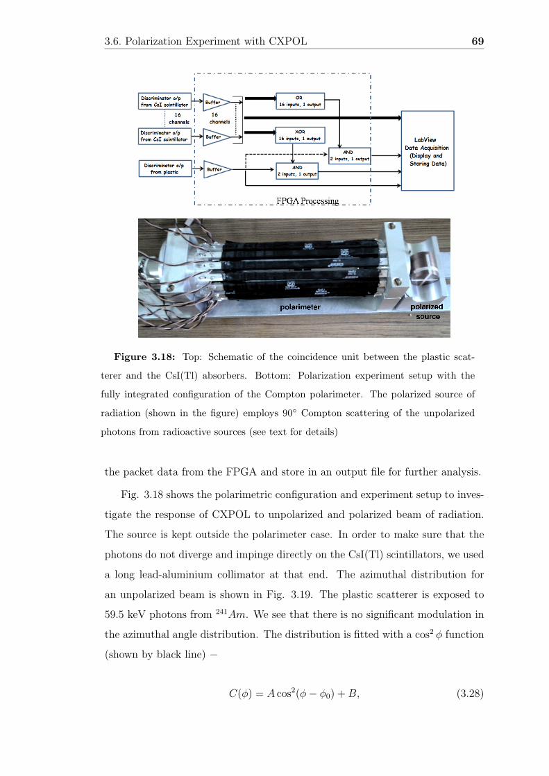
3.6. Polarization Experiment with CXPOL 69
Figure 3.18: Top: Schematic of the coincidence unit between the plastic scat-
terer and the CsI(Tl) absorbers. Bottom: Polarization experiment setup with the
fully integrated configuration of the Compton polarimeter. The polarized source of
radiation (shown in the figure) employs 90 Compton scattering of the unpolarized
photons from radioactive sources (see text for details)
the packet data from the FPGA and store in an output file for further analysis.
Fig. 3.18 shows the polarimetric configuration and experiment setup to inves-
tigate the response of CXPOL to unpolarized and polarized beam of radiation.
The source is kept outside the polarimeter case. In order to make sure that the
photons do not diverge and impinge directly on the CsI(Tl) scintillators, we used
a long lead-aluminium collimator at that end. The azimuthal distribution for
an unpolarized beam is shown in Fig. 3.19. The plastic scatterer is exposed to
59.5 keV photons from 241Am. We see that there is no significant modulation in
the azimuthal angle distribution. The distribution is fitted with a cos2 φ function
(shown by black line) −
C(φ) = A cos2(φ− φ0) + B, (3.28)

70 Chapter 3. Development of the Focal Plane Compton Polarimeter
Figure 3.19: Azimuthal angle distribution for unpolarized 59.5 keV photons. The
distribution is fitted by a cos2 φ function (see Eq. 3.28) shown by black line
where A, B, and φ0 (angle of polarization) are the fitting parameters. Amplitude
of modulation in the azimuthal angle distribution is given by modulation factor
µ =A
A + 2B. (3.29)
Modulation factor is directly proportional to the polarization fraction of the beam.
The small nonzero modulation in this case is because of slight difference in gains
between the scintillators.
We tested the response of CXPOL to a partially polarized beam of 54 keV,
obtained by 90 scattering of 59.5 keV photons from 241Am. An aluminium rod
was used as scattering element. Both the scatterer and the source were kept inside
a thick lead cylinder with a 2 mm diameter hole perpendicular to the incident
beam direction. Spectrum of the polarized beam as taken by a separate CdTe
(Amptek X123CdTe) detector is shown at the top of the left column in Fig. 3.20.
The broad peak centered around 54 keV is the scattered polarized beam. The
narrow beam at ∼59.5 keV is the Rayleigh scattered photons of the original 59.5
keV photons from 241Am. We estimated the polarization fraction of the beam
numerically. The overall polarization will depend on the energy of the incident

3.6. Polarization Experiment with CXPOL 71
Figure 3.20: Left column: Top - Spectrum (taken from CdTe detector) of po-
larized 54 keV beam obtained by 90 scattering of 59.5 keV photons from 241Am.
Middle and Bottom - Azimuthal angle distribution for the partially polarized 54 keV
beam for polarization angles of 0 and 90 respectively. The solid black line is the fit
to the experimental data, whereas the dashed lines are obtained from simulation for
the setup for polarization fractions of 100% (pink), 70% (red) and 40% (blue). Right
Column: similar to the left column, obtained from 109Cd. In this case, the amplitude
of modulation is less due to the presence of unpolarized lead fluorescence photons (72
and 84 keV) as shown in the spectrum (see text for details)

72 Chapter 3. Development of the Focal Plane Compton Polarimeter
photons and the geometry of scattering of the source. The fraction of polarization
turns out to be ∼75%. When this partially polarized beam is incident on the
CXPOL, we see a clear enhanced modulation for the polarized beam compared
to the unpolarized case at 0 and 90 polarization angles (see left column of Fig.
3.20). Different polarization planes are achieved by rotating the lead cylinder
with respect to the plastic axis. First we take background data for long exposure
which is then subtracted from source data. The modulation patterns are fitted
with cos2 φ function (see Eq. 3.28) shown by solid black line. Modulation factors
for both the polarization angles are found to be ∼0.35. To compare the fitted
modulation factors with simulation results, we performed Geant−4 simulation
for the current configuration of the polarimeter. Modulation factor for 100%
polarized 54 keV beam (µ100) is found to be ∼0.50. The conventional way to
obtain the degree of polarization of any partially polarized beam is to take ratio
of the experimentally obtained modulation factor µexpt to the simulated µ100 i.e.
P =µexpt
µ100
. (3.30)
This results in a polarization fraction of ∼70 ± 8%, which is in good agreement
with the numerically estimated value for the 54 keV polarized beam. This is
also demonstrated in Fig. 3.20, where the modulation curves obtained from
simulation are shown in dashed lines, where pink, red, and blue denote 100%,
70%, and 40% polarization respectively. The experimental data agree well with
the 70% polarized signal, as expected.
We repeated the same experiment with partially polarized beam from 109Cd
source. The plot at the top of the right column of Fig. 3.20 shows the spectrum
of this beam centered around 75 keV (90 scattering of 88 keV photons from
109Cd). These 88 keV photons induce fluorescence emission (72 keV and 84 keV)
from the surrounding lead enclosure as seen in the spectrum. These unpolarized
photons are expected to decrease the polarization fraction of the beam. Eventual
polarization degree is expected to be ∼38% in this case, estimated taking into
account the area under the 72, 84 and 75 keV peaks. The modulation curves for
0 and 90 polarization angles are shown in the right column of Fig. 3.20, along
with the modulation patterns obtained from simulation for different polarization

3.6. Polarization Experiment with CXPOL 73
fractions. Modulation factors are found to be low (∼0.20) indicating the beam is
∼40% polarized.
To further test the polarimetric performance of CXPOL at lower energies, we
used an X-ray gun (Amptek Mini-X X-Ray Tube with Gold target) to obtain a
continuum polarized beam. The X-ray gun emits in 10 − 50 keV range. The
lower energy photons (≤ 20 keV) are blocked using a thin aluminium filter. We
employed a similar method to polarize the continuum emission from the X-ray
gun. An aluminium scatterer inside a lead cylinder was kept at the end of the gun
tube (see Fig. 3.21). A small opening of 2 mm diameter ensures that the photons
scattered at 90 can only reach the plastic scatterer. Spectrum of the polarized
Figure 3.21: Left: polarization experiment with CXPOL using continuum radi-
ation from X-ray gun. Right : Spectrum of the polarized 90 scattered radiation of
the gun as taken from CdTe detector
beam as taken from CdTe detector is shown in Fig. 3.21. We see the beam is
continuum in 20−50 keV range. Because of the constrained geometry, we expect
a higher degree of polarization in this case. Modulation curves at 0, 90 and 45
polarization angles are shown in Fig. 3.22. In simulation, we employed a broad
Gaussian beam centered around 35 keV as the source of polarized radiation.
Azimuthal angle distributions for all the polarization planes are found to be
highly modulated consistent with ≥ 90% polarization. All the experiments were
repeated few times to have confidence in the obtained results. The coincidence
time window in the experiments was set to ∼6 µs, it can be altered to a smaller
window of ∼3 µs in order to further improve the signal to noise ratio.

74 Chapter 3. Development of the Focal Plane Compton Polarimeter
Figure 3.22: Azimuthal angle distribution for partially polarized 20−50 keV
continuum radiation for 0 (top left), 90 (top right), and 45 (bottom) polarization
angles. The black solid line is the fit to the experimental data. The pink, red and
blue dashed lines represent the modulation curves obtained from simulation for this
setup for 100, 90 and 80% polarized beams respectively
3.7 Discussions and Future Plans
The main highlights and importance of the experimental results are discussed
below.
• SiPMs have been successfully implemented to read out CsI(Tl) absorbers
for the Compton polarimeter, which helps in designing a compact and op-
timized polarimeter geometry.
• Proper choice of scintillator is extremely important in case of SiPM readout
to have better polarimetric sensitivity. We showed that for CsI(Tl) scintil-
lators viewed by a single SiPM, detection probability degrades significantly
at a distance of 5−6 cm from SiPM at energies ∼50 keV. This is mainly
due to longer scintillation time constant of CsI(Tl) scintillator as a result of

3.7. Discussions and Future Plans 75
which photons reaching SiPM simultaneously are less in number and there-
fore pulse amplitude is low. However, with CeBr3, LaBr3(Ce), NaI(Tl), or
other new generation scintillators, which has comparatively smaller decay
time constant and at the same time similar or even higher light output,
much better performance is expected.
• Choice of appropriate SiPM is also crucial to achieve better sensitivity at
low energies. For lower threshold of the scintillators, SiPMs with less back-
ground (with similar active area) will be useful. Here we used SiPMs pro-
cured from KETEK, which has typical background level of ≤ 500 kHz/mm2.
The new generation SiPMs are supposed to have comparatively much lower
background. Recovery time of the micro-pixels after avalanche is also much
smaller. These are the key factors to obtain a lower energy threshold of 20
keV or less for the Compton polarimeter. We plan to investigate the sen-
sitivity of CeBr3 and NaI(Tl) scintillators coupled to these new generation
SiPMs in near future for the next version of the polarimeter. Coupling be-
tween the scintillator and SiPM is also a key factor for better performance
of the scintillators. We plan for an optimized enclosure for the SiPM and
scintillator which may lead to a better coupling between them and hence
an improved threshold.
• With proper choice of scintillators and optimized scintillator-SiPM cou-
pling, new generation SiPMs can be successfully used for lower energy de-
tections ∼20 keV. This is encouraging as one can now think of new polari-
metric configurations with SiPM in order to have simultaneous polarimetric
and spectroscopic information.
Use of two SiPMs at two ends of a scintillator will not only optimize the
system for better energy threshold but will also give position of interaction
from ratio of pulse heights. In that case, use of a Si detector in place of
the central plastic scatterer will make the instrument sensitive for Compton
spectroscopy in 20 − 80 keV apart from the high resolution spectroscopy
up to ∼40 keV from Si alone. However, the polarimetric performance of the

76 Chapter 3. Development of the Focal Plane Compton Polarimeter
instrument will be compromised because of lower scattering efficiency of Si.
On the other hand, with the use of a 5 mm thick plastic (viewed by SiPM
array) below the SDD, it is possible to greatly improve the polarimetric
performance of the system [100].
Another possible configuration is to use a central scatterer made of seg-
mented plastics with each segment viewed by a SiPM and an array of scin-
tillators with two sided SiPM readout. Such a configuration will optimize
the instrument for polarimetry and Compton spectroscopy in 20 − 80 keV.
The overall energy resolution of the system would be limited by resolution of
the absorbers and uncertainties in constraining the positions of interactions.
However, compared to the Si scatterer configuration, the disadvantage of
this configuration is the infeasibility of photoelectric spectroscopy at lower
energies.
3.8 Summary
We are developing a proof of concept laboratory model of a hard X-ray focal plane
Compton polarimeter, as a foundation for a future proposal of a dedicated hard
X-ray polarimetry mission. The main objective here is to demonstrate a mature
readiness level of a robust polarimeter configuration and to obtain firm estimates
of the resources requirements (in terms of size, weight, power etc) for the future
space experiment. In this chapter, we demonstrated the characteristics of the
plastic scatterer, specifically at the lower energy depositions. We find that detec-
tion efficiency of the plastic is 100% for energy depositions greater than ∼7 keV,
and gradually decreases for lower energy deposition. In the final experimental
configuration of the Compton polarimeter, 16 CsI(Tl)-SiPM systems have been
used to record the azimuthal angle distribution. We characterized each of the
CsI(Tl)-SiPM systems and finally successfully assembled full polarimeter config-
uration and test it with both unpolarized as well as partially polarized X-rays.
The results presented here are expected to be very useful for designing of fu-
ture Compton polarimetry experiments with SiPM scintillator read out systems.

3.8. Summary 77
While this is only a first version of the proposed polarimeter configuration, we
could identify few issues with the initial design, which we plan to rectify in the
subsequent versions.


Chapter 4
Prospects of Hard X-ray
Polarimetry with Astrosat-CZTI
In last two chapters, we described the development of an optimized hard X-ray
Compton polarimeter at the focal plane of a hard X-ray telescope. Whereas
such an approach is expected to magnify the polarimetric sensitivity of the in-
struments by a significant margin in hard X-rays, there is another approach to
extract polarization information from instruments, not optimized for polarime-
try applications, but could be sensitive to it. In this chapter, we describe the
prospects of hard X-ray polarimetry for one such instruments, Cadmium-Zinc-
Telluride Imager (CZTI) on board Astrosat [88,89], Indian multi-wavelength as-
tronomy mission, launched on September 28, 2015. Exploring the possibility of
polarization measurements from CZTI or other similar instruments is particularly
important in the context that there is not a single approved dedicated polarimetry
mission in coming years.
In the last decade or so, there have been many proposed missions as well as
balloon borne experiments [64,65,68,95,112–114], with some of them being con-
sidered at an advanced stage of selection [115]. With the growing realization that
a dedicated polarimetry mission would provide quite fresh results, a dedicated
X-ray polarimetry mission GEMS [66] was selected for development as part of
the NASA Small Explorer program in 2009, but was discontinued in 2012 due
to programmatic reasons. It has been proposed again at the 2014 SMEX NASA
79

80 Chapter 4. Prospects of Hard X-ray Polarimetry with Astrosat-CZTI
call, which has also attracted two more proposals dedicated to X-ray polarimetry,
indicating enhanced interest of community in having firm X-ray polarization mea-
surements. Still, in the absence of any approved dedicated polarimetry mission, it
is very important to explore any possibility of obtaining meaningful X-ray polar-
ization measurements from instruments designed for other related purposes (like
X-ray timing and spectroscopy) and to have a robust ground based calibration.
There have been many attempts to retrieve polarimetric information from
the existing X-ray instruments having notional polarimetric sensitivity, the noted
results being measurement of highly polarized emission from a GRB with the
RHESSI mission and from two Galactic X-ray sources (Cygnus X-1, a black hole
binary and Crab, a pulsar wind nebula) with the IBIS and the SPI instruments on-
board the INTEGRAL mission [15–17,80]. These measurements, however, faced
some criticism because these instruments are not fully optimized for polarime-
try and particularly because their polarimetric capabilities were not calibrated
before launch [28, 86]. Despite limited polarimetric sensitivity of these instru-
ments, the polarization measurements still provide significant insights into the
hard X-ray emission processes in those sources. Therefore, besides attempting
for optimized polarization experiments, it is equally important to explore the
feasibility of X-ray polarization measurements from non-optimized spectroscopic
instruments whenever possible.
CZTI on board Astrosat (see Fig. 4.1), which is primarily designed for hard
X-ray imaging and spectroscopy, is one such instrument expected to be sensitive
to polarization of the incident X-rays due to its large pixelated detector plane.
CZTI is a coded aperture mask telescope with a total active area of 1024 cm2.
The detector plane consists of 64 detector modules arranged in four identical
quadrants, each having 16 modules arranged in a square geometry. Each module
is an independent CZT (Cadmium-Zinc-Telluride) detector with a 16×16 array
of pixels, each of size 2.5 mm×2.5 mm. The 5 mm detector thickness provides de-
tection efficiency at energies higher than the primary spectroscopic energy range
of 10 − 100 keV, where significant fraction of photon interaction is by means
of Compton scattering. In such events, the Compton scattered photon could

4.1. Compton Polarimetry with Pixelated Detectors 81
Figure 4.1: The assembled CZTI payload onboard Astrosat
be detected in an adjacent pixel. Since the direction of the scattered photon
depends on the polarization direction of the incident photon, such pixelated de-
tectors can in general, and Astrosat-CZTI in particular, be used as a Compton
X-ray polarimeter. In this chapter, with experimental and simulation studies, we
show that the Cadmium-Zinc-Telluride Imager (CZTI) on board the forthcoming
Indian astronomy mission Astrosat will be capable of measuring polarization of
the incident X-rays in the energy range 100 − 300 keV. In the next section, we
discuss basic principle of X-ray polarimetry with CZTI. Following this, we discuss
the overall polarimetric sensitivity of CZTI with polarimetric background in Sec.
4.4. Sec. 4.5 discusses the polarization experiment with CZTI and the results
demonstrating the polarimetric capability of CZTI. Finally, the astrophysical sig-
nificance of the polarimetric capability of CZTI is described in Sec. 4.6 before
concluding in Sec. 4.7.
4.1 Compton Polarimetry with Pixelated De-
tectors
When a polarized beam of X-ray photons is Compton scattered, it is preferentially
scattered perpendicular to the direction of polarization, giving rise to a modula-

82 Chapter 4. Prospects of Hard X-ray Polarimetry with Astrosat-CZTI
tion in the azimuthal angle with a cos2 φ variation with the modulation amplitude
directly proportional to polarization fraction of the incident beam. Compton po-
larimetry with pixelated detectors works on the same principle. Here the double
pixel events arising from the Compton scattering of a photon in one pixel and
absorption of the scattered photon in another pixel constitute the basic polariza-
tion event. The azimuthal angle of the Compton scattering is determined from
the direction of center of the scattering pixel to the center of the absorbing pixel
with reference to a pre-defined instrument reference plane. The histogram of the
azimuthal angle distribution can then be used to determine the modulation factor
and polarization angle as usual. It is to be noted that in case of pixelated detec-
tors, the azimuthal angle bins are unequal which leads to an inherent modulation
pattern in the azimuthal angle distribution. Thus the observed modulation pat-
tern has to be normalized using the similar modulation pattern for unpolarized
beam as discussed later.
Astrosat-CZTI consists of an array of pixelated CZT detectors with pixel size
of 2.5 mm (see Fig. 4.2). Timing resolution of CZTI being 20 µs, simultaneous
Figure 4.2: Left: A single CZTI module procured from Orbotech Medical Solu-
tions. Dimension of the module is 40 mm × 40 mm. Thickness is 5 mm. Right: CZTI
module is pixelated into an array of 16 × 16 pixels, therefore pixel size of 2.5 mm
events can be determined with minimum of 20 µs time window. As the CZT
detectors with 5 mm thickness has significant Compton scattering efficiency at
energies > 100 keV, it is expected that Astrosat-CZTI can provide useful polar-
ization measurement at energies even beyond its primary energy range. Though
this configuration of CZTI in principle should be capable of polarization mea-

4.2. Multi-pixel Detection Capability of CZTI Detector Modules 83
surement, feasibility of Compton polarimetry with CZTI depends on many other
factors, namely,
• whether the Orbotech CZTI modules have multi-pixel detection capability
or not,
• if the modules do have multi-pixel detection capability then whether CZTI
will have any meaningful polarimetric sensitivity,
• finally, whether the polarimetric information is preserved by the onboard
data processing.
We experimentally verified the multi-pixel detection capability of the CZTI
modules and carried out detailed Geant−4 simulation for such pixelated CZT
detectors to estimate the polarimetric sensitivity of Astrosat-CZTI. We also car-
ried out polarization experiments to verify the capability of the CZTI processing
electronics to preserve the polarimetric information, which are discussed in the
following sections.
4.2 Multi-pixel Detection Capability of CZTI
Detector Modules
4.2.1 Experiment setup
In order to verify multi-pixel capability of CZTI modules, we conducted an exper-
iment in which 1 CZTI module was illuminated with a partially polarized beam
of energy ∼100 keV.
The experiment setup is shown in Fig. 4.3. Polarized beam of 100 keV
photons was produced by Compton scattering of 122 keV line of 57Co from a
plastic scatterer constraining the angle of scattering at 90. Scatterer, placed in
front of 57Co is 6 cm in length. Both the plastic scatterer and source are kept
inside a thick lead (thickness 2 cm) cylinder with a narrow slit of dimension 5 cm
× 5 mm. CZTI module was kept at angle 90 with respect to the axis of cylinder

84 Chapter 4. Prospects of Hard X-ray Polarimetry with Astrosat-CZTI
Figure 4.3: Schematic diagram of the experiment setup. 122 keV photons from
57Co are scattered at 90 by a plastic scatterer and interact with CZTI module
as shown in Fig. 4.3. Alignment of the slit and the CZTI module was carefully
done from the pixel image of the module.
Since, radioactivity is a random phenomenon, time interval between two suc-
cessive independent events recorded in CZTI module can be modelled by Poisson’s
statistics. However, Compton scattering of an incident photon results in multiple
interactions due to the deposited energies in Compton scattering and subsequent
absorption of the scattered photon, either in the same pixel or separate pixels.
These events, being correlated to each other, should deviate from the modelled
Poisson’s distributed time intervals.
4.2.2 Data analysis and results
Fig. 4.4 shows the histogram of time intervals between two successive events.
There is clearly an excess of events with time interval below 40 µs beyond which
the ∆T distribution agrees nicely with the Poisson’s distribution. Each event has
an individual time stamp with a resolution of 20 µs. Any two events recorded
within duration of 20 µs will have the same time stamp. Therefore the genuine
multi-pixel events i.e. those resulting from the Compton scattering or escape
events in the photoelectric interaction should occur in the same time bin of 20
µs. We observe significant excess in the second time bin (events occurring between

4.2. Multi-pixel Detection Capability of CZTI Detector Modules 85
Figure 4.4: Distribution of time intervals of all successive events recorded in CZTI
module in 57Co experiment. There is an excess of events for time interval below 40
µs. The events beyond 40 µs time interval have been fit with a Poisson’s function
shown by solid red line
20 µs to 40 µs), however, this is due to the specific read-out logic implemented in
the CZTI and is well understood. The detector modules can detect multi-pixel
events and store them internally. The time stamp to each event is assigned after
being read-out. Since the read-out logic is configured to read event from one
module at a time, it is quite possible that two simultaneous events in different
pixel of a given module may get two consecutive time stamps, which results in
excess events in the second bin of the ∆T distribution. Thus, we believe that a
large fraction of the excess events recorded within 40 µs are true simultaneous
events. We have repeated the same experiment with other modules and found
similar results. This clearly shows that the CZTI modules do have capability to
detect and record multiple simultaneous events.
It should be noted that 40 µs is significantly large duration for being consid-
ered as simultaneous and thus could result in many chance coincidence events. In
fact, we do observe successive events in the same pixel with two consecutive time
stamps which are clearly chance events. In order to properly identify such chance

86 Chapter 4. Prospects of Hard X-ray Polarimetry with Astrosat-CZTI
Figure 4.5: Spectra obtained for all double pixel events from 57Co experiment.
Black and red refer to two pool of pixels. For details, refer to text
events and ignore them, we check time stamps of up to five events at a time (we
start with one event and compared the time stamp, ti, of that event with time
stamps of next subsequent events, ti+1, ti+2.., until the difference in time arrival
is > 40 µs) and list all double, triple or more pixel events. We do find a small
fraction of three (or even four) pixel events occurring within 40 µs, however all
such events are ignored and only double pixel events are considered for further
analysis. Fig. 4.5 shows the spectra for the valid double pixel events. Each
valid event involves two pixels; in case of Compton scattering, the pixel with less
deposited energy is the primary pixel and the other one is the secondary pixel.
However, since the module is illuminated uniformly, it is not possible to identify
primary and secondary pixels apriori. Hence, channel histogram for both the
pixels, denoted by black and red, is shown in Fig. 4.5.
This spectra appears similar to the spectra obtained by the direct exposure
of X-rays from 57Co, with both the peaks corresponding to the 122 keV and 136
keV lines clearly visible. This is because of the fact that all double pixel events
are dominated by the chance coincidence events, occurring due to relatively large

4.2. Multi-pixel Detection Capability of CZTI Detector Modules 87
Figure 4.6: Left: Spectra for the neighboring double pixel events. Right: spec-
tra obtained after applying ratio condition (ratio of deposited energies ≥ 2) on the
neighboring double pixel events
coincidence window of 40 µs, of widely separated and independent single pixel
events. Since the Compton scattered photon is not expected to travel far from the
scattering pixel before getting absorbed, we consider double pixel events occurring
only within the adjacent pixels to avoid the chance coincidence events. Left plot
of Fig. 4.6 shows the spectra of the two pixels for all adjacent double pixel events.
It can be seen that majority of chance coincidence events, manifested by the 122
keV and 136 keV peaks, are now absent. However, a small fraction of such events
are still present. To prevent even this small fraction of the chance coincidence
events, we impose another condition on the ratio of the energy deposited in the
two pixels of the adjacent double pixel events. For a true Compton scattering
event, energy of the scattered photon is always greater than the recoil electron
energy for incident photon energies < 280 keV, even for maximum scattering
angles. For lower energy of the incident photons and scattering angles around
90, the ratio of the energy of the scattered photon and the recoil electron is ≥ 2.
Therefore, we consider only those adjacent double pixel events which satisfy this
condition. Right plot of Fig. 4.6 shows spectra of both pixels after applying the
ratio condition. This is the graphical representation of the multi-pixel detection
capability of the CZTI modules. It can be seen that the ratio condition is also
helpful in rejecting other chance events arising from the electronic noise. The
first peak in the spectra corresponds to the primary Compton scattering pixels
and the second peak corresponds to the absorption of the scattered photons.

88 Chapter 4. Prospects of Hard X-ray Polarimetry with Astrosat-CZTI
Figure 4.7: Simulated diagram for a CZT module (40 mm × 40 mm × 5mm).
The module is made to shine uniformly by X-ray photons shown in green
It should be noted, however, that these events may not be pure Compton
scattering events as the escape photons from CZT can also mimic the Compton
scattering and hence the same distribution is also possible for the double pixel
events arising from the detection of the escape photons. In order to estimate the
fraction of such events and estimate polarimetric sensitivity of CZTI, we carried
out detailed Geant−4 simulation as described in the following section.
4.3 Geant−4 Simulation
We used Geant−4 toolkit [96] to estimate modulation factor and efficiency of a
single CZTI module for 100% polarized beam. CZTI module’s electronics ULD
is around 250 keV. For a 5 mm thick CZT, probability of Compton scattering
becomes significant beyond 100 keV. So, simulation was done for mono-energetic
100% polarized and unpolarized beams in the energy range of 100 keV to 300 keV,
employing low energy electromagnetic processes e.g. G4LowEnPolarizedPhotoElectric,
G4LowEnPolarizedRayleigh, G4LowEnPolarizedCompton, G4LowEnBremss and
G4LowEnIonization. The incident beam of photons was generated using General
Particle Source (GPS) which was perpendicularly incident on a single CZT block
(40 mm × 40 mm × 5mm) as shown in Fig. 4.7. For each energy, we carried out

4.3. Geant−4 Simulation 89
simulation for 10 million photons incident on CZT uniformly across its surface
and for each energy, the polarization angle was varied from 0 to 90 at a step of
11.25. For each photon, maximum of 7 secondary photon interaction positions
and corresponding deposited energies were recorded. Deposited energy for each
of such interactions is calculated by summing up the individual energies of all the
secondary electrons generated in that interaction. We ignore the electron track
lengths and assume that total energy of the secondary electron is deposited at
the location of the photon interaction. Output is kept in the form of an event
list with different types of interactions, positions of interactions (maximum 7),
energy deposited in each interaction etc.
4.3.1 Estimation of polarimetric efficiency
Further data analysis was done using IDL (Interactive Data Language). Since
pixel size of Astrosat-CZTI modules is 2.5 mm, the interaction positions in the
event list are pixelated with 2.5 mm spacing. For multiple photon interactions
occurring within the boundary of a single pixel, energies deposited in these inter-
actions are added together to get the total energy deposition in the given pixel.
In this way, we divide all events in single pixel, double pixel, three pixel up to
maximum 7 pixel events. Fig. 4.8 shows the probabilities of the single, double
and multiple pixel (≥ 3) events as a function of incident photon energies. As
only the double pixel events are useful for the polarization measurement, further
analysis is carried out only for the double pixel events. Fig. 4.9 shows the proba-
bility of different types of interactions giving rise to the double pixel events. We
see that apart from the valid Compton scattering events (1 Compton and 1 pho-
toelectric) providing the polarimetric information, there are many other types of
double pixel events which may contaminate the azimuthal distribution of the real
Compton scattering events and blur the polarization signature embedded in the
incident beam. Pure photoelectric events (shown in blue) are because of detection
of an incident photon in one pixel due to photoelectric absorption and detection
of the consequent escape photon (∼30 keV) in another pixel. Probability of these
events is quite significant (∼1%). On the other hand, a photoelectric absorption

90 Chapter 4. Prospects of Hard X-ray Polarimetry with Astrosat-CZTI
Figure 4.8: Probability of single pixel (red, diamond), double pixel (pink, triangle)
and more than double pixel events (green, square) as a function of photon energies
for 2.5 mm pixel size. Total interaction probability for 5 mm thick CZT is shown in
blue (asterisks)
Figure 4.9: Different processes generating double pixel events: photo-photo (blue,
asterisks), 1compt-photo (pink, diamond), 1compt-1photo (red, triangle), photo-multi
compt (green, square), photo-brem (yellow, diamond), photo-brem-compt (light blue,
triangle)

4.3. Geant−4 Simulation 91
Figure 4.10: Spectra obtained from simulation of 200 keV beam. Black and blue
refer to primary and secondary pixels respectively. Top-left: ideal Compton events;
Top-right: all double pixel events; Bottom-left: photoelectric escape events; Bottom-
right: photoelectric-bremsstrahlung events
may lead to bremsstrahlung photons from the ejected electron, detection of which
may trigger double pixel events (shown in yellow and light blue). All these events
may mimic the true Compton scattering events and jeopardise the polarization
signature in the beam.
To obtain spectra for these double pixel events, we assumed the pixel with
lower energy deposition to be the primary pixel i.e. where the Compton scattering
takes place and the pixel with higher energy deposition to be the secondary
pixel in which the scattered photon is absorbed. This assumption holds good
for incident photons with energies up to 280 keV. Representative spectra of true
Compton events and other double pixel events for the incident photons of 200
keV are shown in Fig. 4.10. Spectra shown in black and blue are for primary and
secondary pixels respectively. Spectra for pure photoelectric events shows two
peaks at lower and higher energies due to escape photons. The upper left panel
shows spectra of double pixel events of ideal Compton events and the upper right

92 Chapter 4. Prospects of Hard X-ray Polarimetry with Astrosat-CZTI
Figure 4.11: Azimuthal angle distribution for 200 keV beam with polarization
angle of 0. Left: ideal Compton events. Right: all double pixel events with 20 keV
threshold
panel shows spectra of all double pixels events with minimum energy deposition
above the detection threshold (20 keV) i.e. without any selection on interaction
type. The bottom panels show spectra for only photoelectric escape events (left)
and photoelectric+bremsstrahlung events (right). It should be noted that these
are the spectra of only deposited energy in the pixels and are not convolved for
the CZT detector response.
4.3.2 Estimation of modulation factor
Using pixel map for the double pixel events, we obtained the azimuthal angle
for each of the events. Representative azimuthal distribution corresponding to
the incident photon energy of 200 keV and polarization angle of 0 are shown in
Fig. 4.11, where the top panel shows the azimuthal angle distribution for ideal
Compton events (1 Compton and 1 photoelectric) and the bottom panel shows
the same for all double pixel events with 20 keV threshold in the CZTI module.
It is to be noted that azimuthal angle distribution has an inherent modulation
pattern due to the unequal bin size with respect to the primary pixel i.e. the
azimuthal angle covered by the edge pixels is much larger than that for corner
pixels and hence more number of photons are detected in edge pixels. Since the
polarization direction is parallel to the direction of edge pixels, the counts in
the edge pixels are modulated whereas for corner pixels have the same average

4.3. Geant−4 Simulation 93
Figure 4.12: Spectra (left) and azimuthal angle distribution (right) obtained from
simulation of 200 keV beam (polarization angle of 0) considering the adjacent double
pixel events including the criteria of ratio of deposited energies greater than 2
number of counts. Modulation factor in this case (0 polarization angle) can be
estimated from the events corresponding to 0 and 90 bins or 180 and 270 bins.
Estimated modulation factor for the ideal Compton events is, µ = 0.36, whereas
for all the double pixel events it is, µ = 0.25. The modulation factor for all events
is clearly degraded compared to the true Compton events due to the false events
arising because of photoelectric and bremsstrahlung interactions.
In the previous section, we discussed two conditions derived from the exper-
imental data i.e. considering only adjacent pixel events and ratio of scattered
to deposited energy ≥ 2. In order to get realistic estimate of the modulation
factor from the simulated data, we apply the same conditions to the simulated
double pixel events without using the knowledge of the underlaying interactions.
Fig. 4.12 shows the spectra and azimuthal angle distribution for the double pixel
events on the basis of these conditions.
It can be seen that the modulation factor after applying these two conditions,
µ = 0.23, has slightly degraded from the original modulation factor obtained by
including all events into calculation. This is because of the second condition of
ratio of energy deposited in two pixels to be ≥2, which actually rejects some valid
Compton events where the scattering angle is greater than ∼120 as shown in
Fig. 4.13.
This in turn introduces asymmetry in the range of scattering angle around
90 and thus the effective modulation degrades. Another negative effect of these

94 Chapter 4. Prospects of Hard X-ray Polarimetry with Astrosat-CZTI
Figure 4.13: Ratio of Compton scattered photon energy to electron recoil energy
as a function of scattering angle and incident photon energies. The photon energies
mentioned in the plot are in keV unit
conditions is to reduce the detection efficiency of the Compton events. However,
both these conditions are essential in order to reduce other noisy events, as shown
by the experimental data and hence the expected sensitivity is estimated using
all these conditions.
It is to be noted that the overall degradation in modulation factor is mainly
because of the escape photons which may be avoided by applying energy threshold
of 35 keV in both primary and secondary pixels. With this condition the modu-
lation factor increases from 23% to 41% at 200 keV for polarization angle of 0.
However, this condition restricts the lower energy detection limit of polarization
to be around 150 keV (see Fig. 4.14), thereby reducing the overall polarimetric
sensitivity of the instrument.
As mentioned earlier, the azimuthal bins are asymmetric for the pixelated
detectors and hence the azimuthal distribution has inherent modulation pattern.
This inherent modulation pattern can be corrected by normalizing the azimuthal
distribution with respect to the azimuthal distribution for unpolarized beam at
the same energy (or energy range) [19, 21]. If Ni,pol is the number of counts
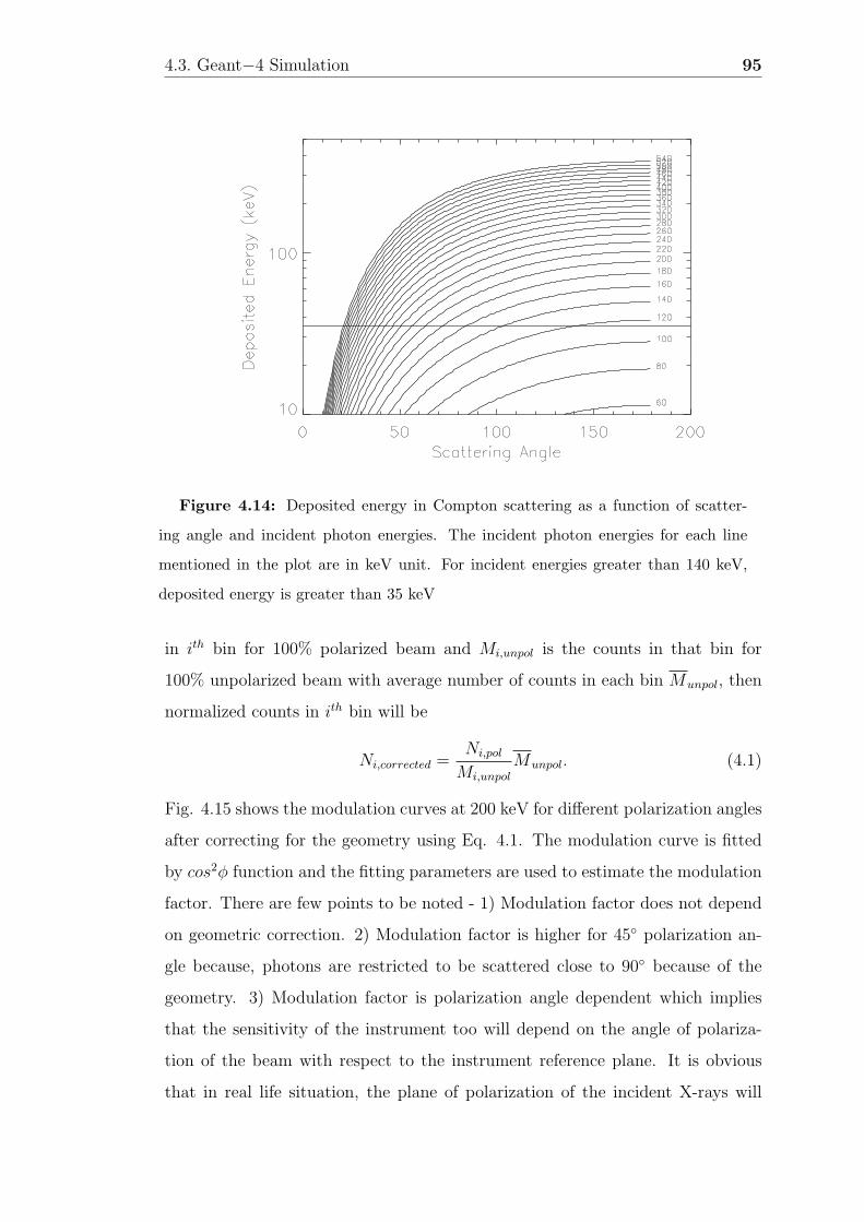
4.3. Geant−4 Simulation 95
Figure 4.14: Deposited energy in Compton scattering as a function of scatter-
ing angle and incident photon energies. The incident photon energies for each line
mentioned in the plot are in keV unit. For incident energies greater than 140 keV,
deposited energy is greater than 35 keV
in ith bin for 100% polarized beam and Mi,unpol is the counts in that bin for
100% unpolarized beam with average number of counts in each bin Munpol, then
normalized counts in ith bin will be
Ni,corrected =Ni,pol
Mi,unpol
Munpol. (4.1)
Fig. 4.15 shows the modulation curves at 200 keV for different polarization angles
after correcting for the geometry using Eq. 4.1. The modulation curve is fitted
by cos2φ function and the fitting parameters are used to estimate the modulation
factor. There are few points to be noted - 1) Modulation factor does not depend
on geometric correction. 2) Modulation factor is higher for 45 polarization an-
gle because, photons are restricted to be scattered close to 90 because of the
geometry. 3) Modulation factor is polarization angle dependent which implies
that the sensitivity of the instrument too will depend on the angle of polariza-
tion of the beam with respect to the instrument reference plane. It is obvious
that in real life situation, the plane of polarization of the incident X-rays will

96 Chapter 4. Prospects of Hard X-ray Polarimetry with Astrosat-CZTI
Figure 4.15: Modulation curves at 200 keV for polarization angles (from upper
left to lower right) of 0, 22.5, 45 and 90. The modulation curves are fitted by
the red solid lines. Modulation factors and efficiencies for different polarization angles
have been mentioned in the respective plots
not be known. Therefore, the dependence of polarization measurement on the
incident polarization angle means that X-ray polarization for any celestial source
measured by Astrosat-CZTI must be verified at different instrument angles with
reference to the measured polarization angle. This can be achieved either by the
rotation of the spacecraft with respect to the source direction or by observing the
same source at different time which may have different spacecraft position with
respect to the source. Another important point to note is that the geometric
correction in the raw azimuthal angle distribution introduces an additional sta-
tistical uncertainty in the modulation factor. As the azimuthal angle distribution
of the unpolarized photons can be estimated very accurately, the uncertainty in
the corrected modulation factor is determined mainly from the statistical uncer-
tainty of the observed azimuthal angle distribution. For sufficiently large number
of unpolarized photons (∼109), we find that the uncertainty introduced by the
correction is less than 0.3%. However, this additional uncertainty in modulation

4.3. Geant−4 Simulation 97
factor should be carefully taken into account because it sets the lower limit for
the overall uncertainty in the measured polarization for any unknown beam.
Fig. 4.16 shows the angle dependent modulation factors and detection effi-
ciency as a function of incident photon energy. It can be seen that the modulation
Figure 4.16: Modulation factor and efficiency (for 100% polarized beam) as a
function of photon energy and polarization angle. Different polarization angles are
denoted by different colors. In the modulation factor vs. energy plot, the curve at
the top corresponds to 45 polarization angle. It is followed by 33.75 and 56.25,
22.5 and 67.5, 11.25 and 78.75 and 0 and 90 polarization angles respectively.
Polarimetric efficiency is independent of polarization angle
factor is maximum for 45 and minimum for 0 and 90. Since scattering geom-
etry is symmetric with respect to the polarization angles 0 and 90, 11.25 and
78.75 so on, modulation factor is same at these polarization angles. Probability
of photoelectric interaction being higher at lower energies, modulation factor is
lower at those energies due to the dominance of the escape photons, compared to
that at higher energies. Overall detection efficiency in the energy range of 100 to
300 keV is of the order of 3% and does not depend on the polarization angle as
expected.

98 Chapter 4. Prospects of Hard X-ray Polarimetry with Astrosat-CZTI
4.4 Polarimetric Sensitivity of CZTI
Estimation of MDP for Astrosat-CZTI require accurate knowledge of µ100 - the
modulation factor for 100% polarized X-rays, Rbkg - background count rate and
Rsrc - source count rate, which in turn requires the knowledge of polarimetric
detector efficiency in the energy range of interest. The modulation factor and
the polarimetric detector efficiency are already determined from the Geant−4
simulations (Fig. 4.16) in the energy range of 100 keV to 300 keV. The other
quantities can be estimated as described in the following subsections.
4.4.1 Source count rate
Source count rate (Rsrc) can be estimated directly by integrating the source spec-
trum, which we assume to be Crab like for the present estimation over the effective
collecting area of CZTI. As mentioned earlier, the polarimetric energy range of
CZTI is beyond the primary spectroscopic energy range. Therefore the coded
mask and other support structure of CZTI has significant transparency at those
energies. Thus for an on-axis source, we estimate the total source count rate for
the two cases - one for the open area of 512 cm2 (50% unobscured area of the
coded mask) by integrating the source spectrum convolved with the polarimetric
efficiency, and second for the area of 512 cm2 shadowed by the partly transparent
coded mask by integrating the source spectrum convolved with both the polari-
metric efficiency and the transmission probability of the mask (made of 0.5 mm
thick Tantalum). Following this method, the total count rate for the Crab is
found to be 1.0006 cnt s−1 in the energy range of 100 keV to 300 keV over the
entire detector plane of the CZTI.
4.4.2 Background estimation
Estimation of background (Rbkg) for Astrosat-CZTI is more involved process. It
should be noted that the polarimetric background of interest here is only the
spurious double pixel events satisfying the filtering conditions mentioned in the
previous section. Such spurious double pixel events can arise either from the

4.4. Polarimetric Sensitivity of CZTI 99
chance coincidence of the usual spectroscopic background i.e. the instrumental
background and the cosmic X-ray background (CXB) or these can also arise
from the actual Compton scattering of the CXB photons. In either case, it is
necessary to first estimate the spectroscopic background rate due to the cosmic
X-ray background.
Cosmic X-ray background
Since Astrosat-CZTI has relatively wide field of view (FOV) of 6×6, the cosmic
X-ray background (CXB) within the FOV has significant contribution in the total
event rate in the detector. However, the most important contribution is from the
CXB leaking through the collimators and support structure, because these are
designed only up to 150 keV which is the primary spectroscopic energy range of
CZTI. We use the hard X-ray spectra of the CXB reported by Turler et al. [98] to
calculate both these contributions. The contribution of the CXB within the FOV
is calculated using the same method as for the source with detection efficiency
of 5 mm CZT and is found to be ∼0.0012 cnt cm−2s−1 in 100 keV to 300 keV.
The contribution of CXB outside the FOV is calculated for two sides of CZTI as
the other two sides are shielded by other instruments. Further, this contribution
is also expected to be different in different CZTI modules because all modules
are collimated by 0.2 mm thick Tantalum wall and hence the inner modules has
increased shielding of the collimators of the outer modules. This contribution is
calculated using Eq. 4.2.
NOFFCXB =
∫φ
∫θ> 6
∫E> 100keV
I(E)Aeff T (E, θ, φ) ε(E, θ) dΩ, (4.2)
where, I(E) is hard CXB spectra [98] in cm−2s−1sr−1. dΩ = sin θ dθ dφ is the
solid angle. Aeff = A cos θ is the effective area of the CZTI module. T (E, θ, φ) is
the transmission probability of Ta collimator(s). Total thickness of Ta, a photon
(energy, E) has to pass through to reach a particular module depends on the
module position, angle θ and φ. ε(E, θ) is the detection efficiency of CZT at
energy E; effective thickness of CZT and thus efficiency of CZT depends on the
angle θ. Other support structure made of Aluminum (total thickness of ∼5 mm)
is assumed to be fully transparent for this calculation. We estimated the CXB

100 Chapter 4. Prospects of Hard X-ray Polarimetry with Astrosat-CZTI
events for all the modules with average value of ∼0.0189 cnt cm−2s−1 in 100 keV
to 300 keV. Thus, the total count rate due to both the CXB within FOV and
outside FOV is found to be 0.0201 cnt cm−2s−1.
Background due to chance coincidence
The chance coincidence can be either between two background events or a back-
ground event and source photon or even between two independent source photons.
The rate of such spurious chance coincidence events can be estimated from the
Poisson’s distribution for the total event rate, N cm−2s−1 , in the detector which
includes the source count rate, instrumental background rate and the cosmic X-
ray background count rate. We estimate total count rate for an on axis source as
mentioned earlier, however now using total interaction efficiency of the detector
instead of the polarimetric efficiency. Source photons being detected in CZTI will
depend on source strength and is found to be ∼0.0322 cnt cm−2s−1 in 100 keV
to 300 keV for 1 Crab source intensity.
The instrumental background generally arises due to the secondary particles
generated from the interaction of the high energy cosmic rays with the overall
instrument as well as spacecraft material. During normal operation, most of the
experimental background is expected to be flagged by anti-coincidence unit and
hence rejected. However, for the purpose of calculating chance coincidence, we
consider the actual counts detected in the CZT detectors. Accurate estimation of
instrumental background typically requires simulation with full mass model of the
spacecraft. Here we use an indicative value based on our earlier HEX experiment
onboard Chandrayaan-1 mission. This experiment used similar CZT modules and
the observed background rate was 2 − 3 cnt cm−2s−1 [116]. Based on this, but
considering different space craft structure and orbit for Astrosat, here we assume
a very conservative value of ∼10 cnt cm−2s−1 for the instrumental background.
Based on these considerations, the total event rate, N , in the CZT detector
is expected to be ∼10.0523 cnt cm−2s−1 in 100 keV to 300 keV for 1 Crab source
strength (0.0322 cm−2s−1 from source, 10.0 cm−2s−1 from instrumental back-
ground and 0.0201 cm−2s−1 from CXB). For this event rate, the total chance

4.4. Polarimetric Sensitivity of CZTI 101
coincidence rate i.e. two events occuring within the conicidence time widow, ∆T
= 40 µs in two adjacent pixels can be estimated using Eq. 4.3,
Rchancebkg =
(N a∆T )2
2!e−Na∆TN a × Ndbl−pix × 64. (4.3)
where ‘a’ is twice the single pixel area (Apix) and Ndbl−pix is the total number
of unique combinations of two adjecent pixels for one CZTI module. From the
simple geometric considerations Ndbl−pix is found to be 926 (i.e. 15 combinations
for a single raw and total 16 raws, 15 combinations for single column and total
16 columns similarly for the two diagonal directions). To get chance events for
whole detector plane, the factor 64 is multiplied. The estimated chance events
is ∼9.4055 × 10⁻⁵ cnt s−1. This value is still overestimated as we have not
applied the ratio condition in the chance coincidence events. It can be seen that
the chance coincidence rate is totally dominated by the instrumental background
and despite assuming a very conservative value for the instrumental background,
the total chance coincidence rate is extremely small as expected for a Compton
polarimeter.
Compton scattering of CXB photons
As mentioned earlier, Compton scattering of the CXB photons constitutes a very
important component of the overall polarimetric background. Again here it is
necessary to consider both the CXB within the FOV of CZTI and the CXB out
of the FOV. The contribution of the CXB photons in the FOV can be calculated
with the same method used to estimate the source count rate, Rsrc - i.e. CXB
spectra [98] multiplied with polarimetric efficiency and transparency of coded
mask for 50% obscured area and CXB spectra multiplied with only polarimetric
efficiency for other 50% unobscured area. Total rate of this component is found
to be ∼0.0347 cnt s−1 in 100 keV to 300 keV over the entire detector plane.
Contribution to the background due to Compton scattering of out of FOV CXB
photons can also be estimated Eq. 4.2, however ε(E, θ) has to be replaced by ap-
propriate polarimetric efficiency for off-axis photons. We extended our Geant−4
simulations for off-axis photons with incident angles ranging from 10 to 85 to

102 Chapter 4. Prospects of Hard X-ray Polarimetry with Astrosat-CZTI
estimate the efficiency of getting double pixel events satisfying all experimental
conditions mentioned in previous sections.
Further, this background will vary from module to module due to varying
degree of shielding from the collimators of adjacent modules. The average back-
ground is found to be to be ∼1.0053 cnt s−1. Thus the total background due
to Compton scattering of CXB is RCXBbkg = 1.0400 cnt s−1 and total background,
Rbkg (= Rchancebkg + RCXB
bkg ), affecting the overall polarimetric sensitivity, is found
to be 1.0401 cnt s−1 in 100 keV to 300 keV over the entire detector plane. There-
fore, the total polarimetric background (i.e. total double pixel events passing all
the filtering criteria) is almost the same as the total polarimetric count rate from
Crab.
Earth’s albedo background
So far, in our background calculations, we did not include effect of Earth’s X-ray
albedo which will have significant contribution to the total polarimetric back-
ground due to low earth orbit of the satellite. We assume that the albedo back-
ground is not polarized which is a fair assumption because of the low earth orbit
of Astrosat and resultant azimuthal symmetry in scattering of albedo from the
Earth’s atmosphere. We have modelled the albedo background and included ef-
fective shielding at individual detector module level. This enables us to calculate
module wise polarimetric background as shown in Fig. 4.17 and thus provides
reliable estimate of effective background. The estimated average background is
now ∼1.5 Crab.
One important repercussion of our module-wise background calculation is the
realization that different subsets of CZTI detector plane will have different sen-
sitivities according to the net background for the given subset. This provides a
very powerful handle to cross-verify the actual polarization measurement between
different subsets and thus to have enhanced confidence in the polarization mea-
surement. It should be noted here that due to the availability of event wise data,
all such sub sampling, either in selection of module subset or the energy range
can be carried out at the analysis level and thus does not impose any special

4.4. Polarimetric Sensitivity of CZTI 103
restriction on the actual observation.
Figure 4.17: Left: Polarimetric background in the energy range of 100 – 300 keV
expected for individual detector modules of CZTI. Right: Angle dependent contribu-
tion of diffuse X-ray background to the total background for the innermost (blue) and
outer most module (red) to demonstrate the effect of collimators and module location.
The dashed curves show background without considering module wise collimators.
4.4.3 Results
Since there is no way to distinguish between the double pixel events due to Comp-
ton scattering of genuine source photons and due to CXB and albedo photons,
the large background from CXB and albedo degrades the modulation pattern. To
incorporate this effect, we degrade the simulated azimuthal distribution for 100%
polarized beam, i.e. flatten it in the proportion to the total polarimetric back-
ground expected in each azimuthal bin, assuming that the azimuthal distributions
of the CXB and albedo photons do not have any intrinsic modulation. Effective
modulation factor is then calculated from this degraded azimuthal distribution.
Sensitivity of CZTI in terms of the Minimum Detectable Polarization (MDP)
for Crab like sources is estimated using spurious event rate and degraded mod-
ulation factors for exposure time of 1 Ms. Fig. 4.18 shows the polarimetric
sensitivity of CZTI in terms of MDP as a function of source intensity. Different
colors represent MDP for different modular subsets of CZTI plane. Sensitivity for
inner subsets is higher compared to outer subsets as expected because of higher
background in the outer modules. Since, the modulation factor depends on the

104 Chapter 4. Prospects of Hard X-ray Polarimetry with Astrosat-CZTI
Figure 4.18: Polarimetric sensitivity of CZTI in terms of MDP as a function of
source intensity for exposure time of 1 Ms. The dashed and solid lines represent the
polarization angle aligned with the pixel edges and at 45 respectively with the latter
being more sensitive due to higher modulation factor as expected. Different colors
represent sub-samples of CZTI detector plane as shown in the inset. The black line
represent the overall MDP as mentioned in the text corresponding to average 22.5
polarization and third (green) sub-array
angle of polarization, sensitivity of the instrument is also polarization angle de-
pendent. For a Crab like source, expected MDP is 4% to 10% for 1 Ms exposure
when the polarization angle with respect to the instrument reference is 45 or
135 and 0 or 90 respectively. MDP values for different source intensities (Crab
unit) and different time exposures (1 Ms and 500 ks) are shown in Table 4.1 for
inner 6 × 6 modules. The Soft Gamma Ray Detector (SGD), which is a narrow
field Compton telescope onboard forthcoming Japanese mission Astro-H [117] to
be launched next year, will also have polarization measurement capability based
on Compton scattering principle in 80 − 300 keV [118]. Polarimetric sensitivity of
SGD is significantly better than that of CZTI primarily due to lower background
and lower energy threshold of the instrument 1.
1Astro-H was launched on February 17, 2016. However, according to the Japan Aerospace
Exploration Agency (JAXA), communication with the satellite unfortunately failed on March

4.4. Polarimetric Sensitivity of CZTI 105
Table 4.1: Polarimetric Sensitivity of CZTI
Source intensity (Crab) Time exposure MDP (%)
0.31 Ms 20.0 - 59.0
500 ks 29.0 - 83.0
0.51 Ms 9.0 - 26.0
500 ks 13.0 - 37.0
0.71 Ms 5.5 - 16.0
500 ks 8.0 - 22.5
1.01 Ms 3.5 - 10.0
500 ks 5.0 - 14.0
It can be seen that the polarimetric sensitivity of the Astrosat-CZTI is mainly
limited due to the off-axis background because the collimators and other support
structures are designed for the primary spectroscopic range upto 150 keV only.
The transparent support structure, however, can be used for advantage by at-
tempting polarimetry of off-axis bright X-ray sources or transient events such as
gamma-ray bursts. Particularly in the case of GRBs, it might be more helpful to
keep the lower energy threshold of 35 keV, so as to get higher modulation factor.
The increased polarimetric threshold of ∼150 keV will not result in significant
degradation of the sensitivity due to the intrinsically hard spectrum of GRBs,
whereas the rejection of the escape events will enhance the modulation due to
the intrinsic polarization in the GRB photons available within the short dura-
tion. This can be readily done during the data analysis and does not require any
change in observation mode. We plan to carry out detailed Geant−4 simulations
for the off axis and out of the field of view sources to estimate their impact on the
polarimetric sensitivity as well as to investigate the prospects of GRB polarimetry
with Astrosat-CZTI.
26, 2016.

106 Chapter 4. Prospects of Hard X-ray Polarimetry with Astrosat-CZTI
4.5 Experimental Confirmation
In order to confirm the polarimetric capability of CZTI, we carried out an X-
ray polarization measurement experiment using the actual flight model of CZTI
module ensuring that all properties of flight electronics are also included in the
experiment. We produced a partially polarized beam of X-rays by scattering 356
keV X-rays from the radio-active source 133Ba at ∼90 degrees (see Fig. 4.19).
A 6 cm long Aluminium cylinder was used as a scatterer. The source and the
Figure 4.19: Left: Polarization experiment setup with CZTI. Right: zoomed view
of the setup
scatterer were placed inside a 4 cm thick Lead cylinder with a slit of 5 cm length
and 2 mm width. The CZTI module is kept below the slit such that only the
photons from 133Ba scattered at 90 by the Aluminium scatterer can reach the
CZTI detector. With this setup, the angle of scattering is constrained to 90±15
implying a partially polarized beam of energy between 190 keV and 240 keV.
The basic data filtering and analysis were carried out as discussed in Sec. 4.2.
This involved selection of appropriate adjacent double pixel events, generating
8 bin azimuthal distribution with reference to lower energy pixel and correcting
azimuthal distribution for the unequal angle bins. Fig. 4.20 shows the corrected
modulation curves for partially polarized beam at two different polarization an-
gles, 0 and 45, with reference to one of the edges of the CZT detector module
as well as for an unpolarized beam (direct exposure to 356 keV X-rays). It can
be seen that the modulation curves for the measurements at these polarization
angles show clear signature of the polarization of the incident beam and the

4.5. Experimental Confirmation 107
modulation curves corresponding to different polarization angles also change as
expected. The errors in the observed modulations are nominal 1σ errors and the
simulation results too have errors of similar magnitudes. In the case of the unpo-
larized beam, the residual modulation, which could be due to the instrumental
artifacts, is almost negligible ( 1%) and thus will not have any significant effect
on the polarization measurement aimed at largely polarized source. It should be
noted here that one major criticism of the recent X-ray polarization measure-
ments by INTEGRAL IBIS and SPI instruments is that these instruments were
never tested with an unpolarized beam. These results clearly demonstrate that
Figure 4.20: (a) and (b) Experimentally measured modulation curves for par-
tially polarized X-rays from 133Ba source at two polarization angles 0, and 45 re-
spectively. (c) The same curve measured for unpolarized X-rays from 133Ba. The
dashed line shows the modulation curves obtained from the Geant−4 simulations of
the experimental setup
CZTI is capable of detecting polarization of the incident X-rays. However, the
observed modulation amplitude cannot be directly used to validate the simulation
because of the partially polarized beam. In order to have a quantitative compar-
ison with the simulations, we repeated the simulations for the exact geometry
of the experiment including the generation of the polarized beam and considered
the experimentally measured background to calculate the modulation factor. The
modulation factors obtained from these simulations typically agree within ∼1%
of the experimentally measured modulation factors, in all the cases. This implies

108 Chapter 4. Prospects of Hard X-ray Polarimetry with Astrosat-CZTI
that the value of µ100 obtained from simulations do represent realistic modulation
factor.
4.6 Astrophysical significance of CZTI Polarime-
try
It can be seen from Fig. 4.18 that for a Crab like source, MDP of 5% can
be achieved in exposure time of ∼1 Ms. Though such long exposure times are
routinely quoted in the context of X-ray polarimetry, these may not be realistic for
the observatory class mission such as Astrosat. On the other hand, in the energy
range of interest (100 − 300 keV) the emission from almost all X-ray sources
is expected to be of non-thermal origin and thus can be highly polarized. This
is corroborated by the recent reports of more then 50% polarized soft gamma
emission by INTEGRAL from two bright X-ray sources Crab and Cygnus X-
1 [15–17]. In this context, a more appropriate question is - given highly polarized
X-ray emission, how well its polarization can be constrained by CZTI with a
typical exposure time of few tens of kilo-seconds.
For an unknown source, the polarization degree P is given by -
P =µ
µd,100
, (4.4)
where, µ and µd,100 are the measured modulation amplitude for that source and
the degraded modulation factor respectively. It should be noted that the de-
graded modulation factor µd,100 takes into account the effect of Compton scatter-
ing of the background photons (both cosmic X-ray background as well as albedo
background) as discussed earlier and hence it is smaller then µ100 obtained from
Geant−4 simulations. Error in the measurement is given by
σP
P=
√σ2µ
µ2+
σ2µd,100
µd,1002, (4.5)
where, σµ is the statistical error associated with the measurement of modula-
tion factor µ which depends on both the degree of polarization in the source
and the source intensity. σµd,100is the error in µd,100. It should be noted that

4.6. Astrophysical significance of CZTI Polarimetry 109
σµd,100depends on the relative angle between the polarization direction of the
incident X-rays and a reference direction of the instrument. In general, the po-
larization angle can not be constrained to better than 28.5/(P/σP ) simply by
fitting the modulation curves [119]. Thus in most cases, the uncertainty in po-
larization angle can be assumed to be 15 − 20. Fig. 4.21 shows the detection
significance for different source intensities as a function of exposure time, with
µd,100 and σµd,100corresponding to the average polarization angle of 22.5 and
uncertainty in polarization angle of ±10. It can be seen that for large exposure
Figure 4.21: Detection Significance of polarization measurement for highly po-
larized bright sources. The bottom three lines correspond to 500 mCrab sources with
polarization fraction of 20% (black), 40% (green), 60% (pink) respectively. The top
line (red, dashed) corresponds to 1 Crab source having polarization fraction of 50%
times, the significance of polarization measurement saturates due to the uncer-
tainty in µd,100. However, for smaller exposure times ( 100 ks), the uncertainty
in polarization measurement is dominated by the counting statistics. Since the
large exposure times are expected to be resulting from multiple smaller exposure
times with different position angle of the spacecraft, it is more appropriate to
consider the average polarization angle of 22.5 (this is the angle with reference

110 Chapter 4. Prospects of Hard X-ray Polarimetry with Astrosat-CZTI
to the instrument reference direction and not the absolute polarization angle in
the sky frame). However, in many such cases, it might be possible to have bet-
ter constrains on absolute polarization angle based on multiple smaller subset of
the same data, which may result in higher significance of the polarization mea-
surement. Another factor affecting detection significance of polarization is the
uncertainty in polarimetric background. The shaded regions around lines in Fig.
4.21 represent the variation of significance for probable variation of the polari-
metric background by ±20% for the same statistical and systematic errors. It
can be seen that, even after considering all these uncertainties, for a 500 mCrab
source with 40% intrinsic polarized fraction, the polarization can be measured
with 3σ confidence with an exposure time of 100 − 150 ks.
Since polarization measurements with CZTI are possible only for bright (>
500 mCrab) X-ray sources, the obvious candidates are the two eminent sources
Cygnus X-1, a black hole binary and Crab, a pulsar wind nebula. The fact that
the initial indication of highly polarized emission from both these sources are
available from INTEGRAL observations, makes the astrophysical significance of
CZTI polarimetric capability more relevant.
In the case of Cygnus X-1, measurements by both IBIS and SPI instruments on
INTEGRAL show very high polarization fraction (∼65%) at energies greater than
∼250 keV, which is interpreted in terms of the emission from the base of a jet [15].
While a significant contribution from the jet to hard X-ray / soft gamma emission
has been speculated for some other black hole binaries in literature [25–27], recent
SED modelling of Cygnus X-1 spectral energy distribution by Zdziarski et al. [28],
spanning from radio to MeV range, suggests that significant jet contribution to
hard X-ray emission can be achieved only with rather unrealistic parameters.
On the other hand, there are other models which predict state independent high
polarization [24, 29] as well as moderate polarization only in hard state. Thus
the present scenario of polarized nature of hard X-ray emission from Cygnus
X-1, both fro observations as well as theoretically, is rather confusing and it is
thus important to independently constrain it. In this context, we considered
various available predictions of X-ray polarization for Cygnus X-1 to investigate

4.6. Astrophysical significance of CZTI Polarimetry 111
whether these can be delineated with CZTI , particularly in the presence of some
of the systematic effects such as uncertainty in background, uncertainty in the
knowledge of polarization angle etc. (see Fig. 4.22).
The possible scenarios considered here (denoted by red, green, black and blue
respectively in Fig. 4.22) are − strong polarization signature (∼ 50%) in LHS
(low hard state) due to relatively high jet contribution; comparatively lower po-
larization fraction of 25% because of relatively lower jet contribution in LHS;
∼15% polarization in LHS originated in corona due to inverse Compton scatter-
ing and high polarization (around 55% in high soft state) because of synchrotron
radiation from the corona itself. We found that most of the scenarios can be
constrained rather accurately within an exposure of time of ∼200 ks.
In the case of the Crab nebula, based on the polarization measurements at
other wavelengths (including soft X-rays which is the only historic positive X-ray
polarization measurement from an astrophysical source [2]), it is well known that
the nebular emission arises from synchrotron radiation. However, the mechanism
as well as the geometry of the emission from the pulsar itself are still not fully
understood with various models such as polar cap, outer gap, slot gap, stripped
wind [120, 121], being compatible with all other observational characteristics.
One distinguishing feature of these models is their phase-dependent polarization
signature. The INTEGRAL measurements, folded with the Crab pulse period,
suggests that the polarization is varying at different phases, and thus goes against
the polar cap model. But in order to constrain other models it is necessary to get
truly phase resolved polarization measurements, which typically need an order
of magnitude larger exposure time. Since the Crab is likely to be observed for a
long duration as a standard candle, it is possible that a total exposure of a few
million seconds can be obtained. In such a case, we find that full phase resolved
polarization measurement is certainly possible with the lowest polarization also
constrained better then 3 sigma. As an example, Fig. 4.22 shows the Crab
polarization detection significance, estimated in 16 uniform phase bins. The phase
resolved polarization values used in our calculation are obtained by interpolating
the recent Crab polarization estimates by IBIS [81]. Thus, we see that CZTI can

112 Chapter 4. Prospects of Hard X-ray Polarimetry with Astrosat-CZTI
Figure 4.22: Left: Possible constrains on hard X-ray polarization fraction of
Cygnus X-1 for some of the model predictions proposed in literature (see text for
details), predicting about 15%, 25% and 50% polarization in low hard state (total
flux sin300 mCrab) and about 55% polarization in high soft state (total flux ∼1
crab). Expected errors are shown as shaded regions. Right: Feasibility of phase
resolved polarimetry with CZTI for Crab. The top panel shows Crab pulse profile in
100 300 keV. The middle panel shows polarization in 16 phases as expected from an
interpolation of the polarization measured by INTEGRAL in four regions of Crab pulse
profile. The shaded region represents possible constraints on phase wise polarization
measurement with CZTI for a total exposure time of 1 Ms. The bottom panel shows
the required exposure time to determine polarization for all phases with a minimum
3 sigma (solid lines) and 5 sigma (dashed lines) confidence levels. It can be seen
that with a total exposure time of ∼2 Ms, polarization in most of the phases can be
constrained with better then 5 sigma confidence
provide much better insights into the Crab pulsar emission mechanism.
However, polarimetric studies with CZTI will not be limited to only these
two sources. There are many transient X-ray binaries, which undergo outbursts
lasting from a few weeks to months and have intensities more then 500 mCrab.
Since such transient sources are of general interest, it is likely that at least the
long outbursts will be observed extensively by Astrosat and thus will result in a
total exposure time sufficient for the polarimetric studies with CZTI. Based on
the analysis of long term monitoring data from sky monitors such as RXTE-ASM,
SWIFT-BAT, we find that typically 2 to 3 outbursts which are brighter then 500
mCrab and longer than one week are expected during the period of one year (see

4.7. Summary 113
Table 4.2).
Table 4.2: List of potential sources for CZTI polarimetry obtained from BAT 70
month catalog [122]
Source Name Source TypeON Time
(>300 mCrab)
ON Time
(>500 mCrab)
Crab Pulsar/PWN 100 % 100 %
CygX1 Black Hole HMXB 95.03 % 92.57 %
GX339-4 Black Hole LMXB 3.03 % −−−
XTEJ1752-223 Black Hole LMXB 4.45 % −−−
SWIFTJ1753.5-0130 Black Hole LMXB 1.94 % −−−
SGR1806-20 Magnetar 2.69 % −−−
Thus, given an operational life of 5 years, CZTI is likely to investigate the
presence of highly polarized emission from at least 10 transient sources which are
typically black hole and neutron star binaries.
4.7 Summary
To summarize this chapter, Astrosat-CZTI will have significant polarimetric capa-
bilities. The polarization capabilities are verified on ground, both with partially
polarized beam, and more importantly, with unpolarized beam. This will pro-
vide additional confidence to consider the actual polarization measurements as
intrinsic to the source and constrain various theoretical models based on them.
The GAP (Gamma-ray Burst Polarimeter) instrument, which is a small Compton
scattering based polarimeter onboard a Japanese Small Solar Power Sail Demon-
strator mission IKAROS [123], has demonstrated the importance of robust ground
calibration of polarimeters based on which it is successfully measuring polar-
ization of GRBs. As mentioned earlier the Soft Gamma Ray Detector (SGD)
onboard Astro-H to be launched next year 2, provides significant polarization
2According to recent news, after one month of its launch, communication with Astro-H failed
on March 26, 2016.

114 Chapter 4. Prospects of Hard X-ray Polarimetry with Astrosat-CZTI
measurement capability in hard X-rays [118]. Astrosat-CZTI with much larger
area compared to GAP and much larger field of view compared to SGD, will
prove to be an unique instrument capable of probing the X-ray polarization of
bright celestial sources. Further, Astrosat being an observatory class satellite
with X-ray timing as one of its primary objectives, it is likely to devote a large
fraction of its observing time to bright X-ray binaries, thus facilitating, as an ad-
ditional bonus, measurement of X-ray polarization in the 100 − 300 keV region.
Since at energies beyond 100 keV, the coded mask and supporting structures of
CZTI become more and more transparent, CZTI offers opportunity to attempt
polarization measurements of GRBs which are expected to be highly polarized.
Thus it is likely that the field of hard X-ray polarimetry will witness significant
advances in the near future.

Chapter 5
Generation of Multi-Pixel
Response Matrix for
Astrosat-CZTI
In Chapter 4, we described the prospects of hard X-ray polarimetry with Cad-
mium Zinc Telluride Imager (CZTI) onboard Astrosat. However, it is to be noted
that polarization measurements with CZTI is just an additional bonus, as CZTI
is primarily a coded mask spectroscopic instrument sensitive in 20 − 100 keV
energy range. With proper characterization of the CZT detectors, it is possible
to carry out fine spectroscopic analysis for celestial X-ray sources with CZTI.
Better spectroscopic study of sources and proper interpretation on the emission
mechanisms prevalent at those sources out of the spectroscopic data critically
depends on the response matrix of instrument. So, apart from polarization study
with CZTI, we also worked on the characterization of CZTI detector modules to
generate accurate response matrix of the instrument.
CZT detectors provide high photopeak efficiency in a broad energy band of
few keV to few hundreds of keV, fine energy and spectral resolution at near room
temperature and can be operated in a wide temperature range. It also provides
the sufficient radiation hardness required for any space based experiments. CZT
detectors, for all these reasons, have been boosting hard X-ray astronomy for more
than a decade now, having been used in many X-ray astronomy experiments and
115

116 Chapter 5. Generation of Multi-Pixel Response Matrix for Astrosat-CZTI
missions − SWIFT [124], INTEGRAL [125], NuSTAR [93], EXIST [126], RT-2
experiment onboard CORONAS-PHOTON [92] and planned for future astronom-
ical missions like Astro-H 1 [75], X-Caliber [76] etc. As mentioned earlier, CZTI
onboard Astrosat [89] also uses an array of CZT detector modules. However
unlike other semiconductor detectors (Si, Ge detectors), the X-ray lines due to
mono-energetic X-ray photon interactions in CZT do not feature Gaussian shape
due to incomplete charge collection on the electrodes due to low mobility and life-
time of the charge carriers (electrons and holes). In particular, low mobility of the
holes coupled with very low lifetime causes a significant fraction of charge being
trapped by impurities. Since charge collection depends on the depth of interac-
tion which is a statistical phenomena, there is a long tail at the lower energy side
of an otherwise Gaussian line shape. Since at higher energies, depth of interaction
increases, the tailing effect is also found to be more prominent for high energy
photons. In order to fully utilize the capability of CZT detectors by performing
fine spectroscopic studies out of it, it is important to generate accurate response
matrix. For that, it is necessary to model the CZT line shapes precisely by tak-
ing care of the mobility and lifetime of the charge carriers. Method to predict
CZT line profiles by modelling charge trapping (hereafter, µτ model) has been
discussed in [100, 127]. However, the line profiles become further complicated
when the CZT detectors are pixelated as in case of NuSTAR or Astrosat-CZTI
as charge sharing, Compton scattering between the pixels may also contribute to
the tail of the line.
In this chapter, we demonstrate our modelling results to the line shapes for
5 mm thick CZT crystals with 16 × 16 pixels (2.45 mm pixel pitch) procured
from Orbotech Medical Solutions, similar to the detectors used in CZTI onboard
Astrosat, so that the same method can be implemented for CZTI for response
matrix generation. We found that though µτ model fit the CZT line profile
quite well at higher energies, at lower energies (∼60 keV), proper fitting requires
an additional component in the model − charge sharing between the pixels. It
1According to recent news, after one month of its launch, communication with Astro-H failed
on March 26, 2016.

5.1. CZT Line Model 117
is interesting as provided the small photo-electron range for any X-ray photon
interaction (charge cloud radius) and pixel pitch of 2.45 mm, charge sharing is not
expected to be significant. However, we did extensive experiments to validate our
model and in particular justify the requirement of the charge sharing component
in the model. The numerical models are described in Sec. 5.1 and can be used
for any pixel size of the CZT detector and detector thickness, therefore may
be helpful in characterizing CZT detectors in future astronomy missions as well
besides CZTI. Again one of the key features of the model is that it uses charge
sharing fractions as a fitting parameter and does not consider the complicated
electric field geometry to evaluate the wighting potentials. Therefore, it is possible
to understand the charge sharing process for a given CZT pixel geometry using
these models with the help of optimized experiment setup. In Sec. 5.2, we
describe the procedure to experimentally estimate the µτ products and charge
sharing parameters followed by an experiment to validate the model in Sec. 5.3.
Finally, we summarize our results and future plans in Sec. 5.4.
5.1 CZT Line Model
As discussed earlier, the model consists of two physical components which are
descibed in the following.
Charge trapping: The shape of mono-energetic X-ray line from CZT detectors
depends on µτ product of charge carrier. For a uniform electric field (E) in CZT
crystal, the fraction of charge collected from specific interaction depth is given
by Hecht equation [128],
η =λe
D
[1 − e−
D−xλe
]+
λh
D
[1 − e
− xλh
], (5.1)
where, η is the ratio of induced charge to the initial charge generated after in-
teraction, D is the thickness of the crystal, x is the distance of interaction site
from cathode and λe (=(µτ)eE) and λh (=(µτ)hE) are the mean free paths for
electrons and holes respectively.
We have developed a numerical model to predict line shape from CZT detectors
based on Eq. 5.1, where we divide the CZT crystal in N number of layers along

118 Chapter 5. Generation of Multi-Pixel Response Matrix for Astrosat-CZTI
Figure 5.1: Demonstration of tailing effect in CZT line shape due to charge
trapping (µτ model) for 122 keV photon energies. Different colors denote different µτ
products
its depth where each layer will give rise to a Gaussian with peak energy depending
on the induced charge for that layer. The amplitude of the Gaussian will depend
on the probability of interaction at that layer for the given energy (E0) of the
X-ray photons. All the Gaussian lines are finally added together to obtain the
final line shape, F ,
F =N∑i=1
N0Pie− (E−ηiE0)
2
2σ2i , (5.2)
where, i runs from 1 to N number of slices which we consider to be 100 for our
calculations. N0 is the number of incident photons and Pi is the probability of
interaction at the ith layer for photons of energy E0, given by
Pi = e−µρx(1 − e−µρ(D/N)). (5.3)
σi is the width of the Gaussian which is assumed to be same for all the layers. If
λe and λh are high i.e. values of µτ products are large, η tends to unity (see Eq.
5.1), resulting in a Gaussian shape for the X-ray line. Alternatively, for x ∼ 0, i.e.
interactions occurring close to the cathode η again tends to unity. Therefore, for
low energy photons, we do not expect significant tail compared to higher energy

5.1. CZT Line Model 119
photons. Fig. 5.1 shows the CZT line shapes predicted by the µτ model for 122
keV energy photons for various µτ products. The bias voltage considered here
is 600 V. The line shapes are found to have more prominent tail with lower µτ
product of holes.
Charge sharing: Charge sharing is required for pixelated detectors as the
charge cloud formed after an X-ray photon interaction inside a CZT pixel, will
diffuse due to random thermal motion of electrons and Coulomb repulsion. While
traversing towards the electrode, a fraction of charge cloud may end up to the
neighboring pixels giving rise to an incomplete charge collection. This will con-
tribute to the tail of the line profiles making it further complicated.
We have developed a simple charge sharing model based on the cloud expan-
sion due to random thermal motion of electrons. [129,130] also followed a similar
treatment to account for cloud expansion. Since expansion of the cloud size due
to Coulomb repulsion is insignificant compared to that due to thermal motion of
charge carriers, specially for energies < 200 keV, we ignored the Coulomb forces
in the electron charge cloud. Radius of charge cloud as it drifts across the detec-
tor can be estimated assuming Gaussian distribution of charge concentration as
a function of drift distance (from solution of Fick’s equation),
r = r0 + 1.15
√2kTdD
qV, (5.4)
where, r0 is the initial cloud radius and r is the cloud radius at the end of the drift
d. q is electronic charge and V is the bias voltage. T is the detector temperature
and k is Boltzmann’s constant. r0 is expected to be of the same order of the
photo-electron range in CZT material for incident photon energy of E0. One
can estimate the amount of charge left inside the pixel assuming spherical charge
cloud using Eq. 5.4,
f = 1 − π(r − y)2
3(3r − (r − y))/
4
3πr3, (5.5)
where, y is the position of interaction from the edge of the pixel. The model
essentially implies that for interactions closer to the edge of the pixel, there will
be significant charge loss. As we move towards the center of the pixel, at some
distance from the edge equal to the radius of the final charge cloud, charge loss

120 Chapter 5. Generation of Multi-Pixel Response Matrix for Astrosat-CZTI
will stop. This will give rise to a tailing effect as amount of charge loss will depend
on the interaction site from the edge and on the depth of interaction.
We couple the charge sharing model with the charge trapping by dividing the
CZT detector plane into M number of slices and compute the charge loss for
each slice due to both charge sharing and charge trapping for vertical N slices as
explained earlier. The final model looks like,
F =M∑j=1
100∑i=1
N0jPie−
(E−ηifj,iE0)2
2σ2i , (5.6)
where, j runs from 1 to M number of slices along the plane of CZT, which we
consider to be 2000 for calculations and i runs for 100 slices in vertical direction
along the depth of CZT for a given j. N0j is the number of incident photons in
jth slice and can be considered same for the slices in case of uniform illumination
(N0j = N0/M) or of some other suitable functional form in case of nonuniform
illumination. Fig. 5.2 shows the model predicted CZT line shapes for various r0
(initial cloud radius) values for 60 keV and 122 keV photon energies. Effect of
Figure 5.2: Model predicted CZT line profiles for 60 keV (left) and 122 keV
(right) photon energies for various r0 values. Assumed values of µτ product here are
0.002 and 0.0001 for electrons and holes respectively. The bias voltage is considered
here to be 600 V
increase in charge cloud radius on the line shape is quite evident for both 60 keV
and 122 keV photons. In case of 60 keV photons, the effect of charge trapping on
the tail is insignificant as most of the photons will interact within ∼1 mm from
the cathode. Therefore, the tailing effect is only due to charge sharing. On the

5.1. CZT Line Model 121
other hand, for 122 keV photons, the contributions of both charge trapping and
charge sharing to the tail of the line are quite significant.
It is to be noted that here we only estimate the amount of charge going out of
a given pixel; we do not bother about the amount of charge shared between two
adjacent pixels which will further depend on the anode and interpixel geometry.
Charge sharing from adjacent pixels and interpixel junction may also contribute
to the tail of CZT line shape. The other factors which may have contribution to
CZT line tails are
• Compton scattering from neighboring pixels to the pixel under consideration
as the scattered photons will have energies close to the photopeak energy
depending on the angle of scattering,
• escape of Bremsstrahlung photons (mostly generated from high energy
photo-electrons) and electrons from the pixel will also lead to an incom-
plete charge collection and thus may affect the tail of line shapes.
However, effect of Bremsstrahlung photon escape and electron escape from the
pixel is not very significant. Compton scattering from the adjacent eight pixels
is also insignificant. This is demonstrated in Fig. 5.3, which is obtained from
Geant−4 simulation of a 2.45 mm × 2.45 mm CZT crystal with thickness of 5
mm. The detector plane is uniformly illuminated by 59.54 keV (left) and 122 keV
(right) photons. We see that the number of photons undergoing Bremsstrahlung
escape and electron escape in the energy range 40 − 58 keV (in case of 59.54 keV
photons) is less than 0.3% of the total number of photons incident. The events
below 15 keV are due to Compton scattering. We expect a similar number of
events (actually less as these events are for scattering in all direction) in total
from the neighboring eight pixels surrounding the central pixel. Fraction of these
events is also found to be less than 0.4%. In case of 122 keV incident photons
also, these numbers are found to be insignificant ∼0.2% and <4% respectively.
These events are therefore not significant to contribute to the tail of the lines.
Thus we only model the charge sharing fractions along with the charge trapping
to predict the CZT line shape as function of incident photon energy.

122 Chapter 5. Generation of Multi-Pixel Response Matrix for Astrosat-CZTI
Figure 5.3: Energy distribution for 59.54 keV (left) and 122 keV (right) photons
obtained from simulation for a 2.45 mm × 2.45 mm CZT crystal with 1 million incident
photons. The main peaks in the distribution are the photopeaks and other smaller
peaks correspond to escape photons. The events closer to the photopeak are because
of escape of bremsstrahlung photons and escape of electrons. Events at the lower
energies are the Compton scattered events
5.2 Measurements of µτ Products and Charge
Sharing Fractions
The model (Eq. 5.6) is written in S-LANG and incorporated in spectroscopic
data analysis package, ISIS (Interactive Spectral Interpretation System) as a local
model. There are total six parameters in the model − (µτ)e, (µτ)h, photopeak
energy E0, N0j, spread of the line σ, and initial radius of the electron cloud
r0. In order to constrain µτ product precisely, we fit three spectra at different
energies (59.54 keV line from 241Am, 88 keV line from 109Cd, and 122 keV line
from 57Co) simultaneously tieing up the µτ product across the spectra as µτ
product is expected to be constant for a crystal at a given temperature. It is
to be noted that since the model components are energy dependent, fitting the
model simultaneously for three different energies put tighter constraints on the
model parameters rather than fitting the model for a single energy but at three
different bias voltages.
We use CZT detectors procured from Orbotech Medical Solutions. The de-
tectors are available as integrated detector module having both CZT crystal and

5.2. Measurements of µτ Products and Charge Sharing Fractions 123
the front end readout ASIC. Spectra is acquired by the data collection unit
OMS36G256-SDK provided along with the OMS Detectors Array Unit (see Fig.
5.4). The gain-offset corrected spectra are first binned with a binsize of 0.5 keV
Figure 5.4: OMS Detectors Array Unit and the data collection unit OMS36G256-
SDK
in energy space which are then fitted simultaneously by the CZT line model.
σ, N0j, E0 are kept free while fitting. r0 should depend on the energy of the
incident photons as the charge cloud initial radius can be approximated as the
ejected photo-electron range in CZT material which depends on the energy of
the incident photons. However, the change in radius is not very significant for
increase in photon energy from 60 keV to 122 keV. Again, as discussed earlier
and we will see later, r0 also takes care of other physical factors such as charge
coming in from the adjacent pixels and interpixel junction to the pixel under
consideration, which is expected to contribute to the tail of CZT line shape and
therefore may modify the actual r0 value. Consequently, we may not obtain any
functional form of r0 as a function of photon energy which is necessary to finally
compute the response matrix elements of the detector as a function response en-
ergies. Therefore, we consider r0 to be same for all three energies for a given pixel
while fitting. r0 obtained in this way, is basically the cloud radius averaged over
energy range from 60 to 122 keV.
Another important factor to be noted here that closer to the anode, the electric
field lines will be too dense due to fringing effect to allow further expansion of the
charge cloud. We take care of this by assuming an optimized quenching distance

124 Chapter 5. Generation of Multi-Pixel Response Matrix for Astrosat-CZTI
of 3.5 mm from the cathode such that there will not be any further expansion in
cloud size beyond this distance. This has a significant effect at higher energies
as there is a significant probability of high energy photons to interact beyond
this layer and therefore charge loss will be effectively smaller compared to that at
lower energies (< 60 keV). This argument can be further seconded from the fact
that in polarization experiments with OMS CZT detectors in Astrosat-CZTI, the
experimental modulation factors were found to be very close to the simulation
results in the energy range 190 − 240 keV as discussed in Chapter 4, which implies
that there is no significant charge sharing at higher energies.
Fig. 5.5 shows the obtained fitting for two separate pixels (120th pixel (left
column) and 200th pixel (right column)) at three energies. We see that the model
Figure 5.5: Simultaneous fitting of three spectra for two separate pixels − 120th
pixel (left column) and 200th pixel (right column). The top, middle and the bottom
panel show spectra for 59.54 keV line from 241Am, 88 keV line from 109Cd, and 122
keV line from 57Co respectively
predicts the line shapes very accurately. We fitted spectra for all 256 pixels of a
module and constrain (µτ)e, (µτ)h, and r0 parameters. In Fig. 5.6, we show the

5.2. Measurements of µτ Products and Charge Sharing Fractions 125
distribution of (µτ)e, (µτ)h for the whole module. Typical (µτ)e, (µτ)h values
Figure 5.6: Distribution of (µτ)e (top) and (µτ)h (bottom) with pixels for CZT
detector module. Mean values of (µτ)e, (µτ)h are found to be around 10−3 and 10−4
respectively
are around 10−3 and 10−4 respectively. Fig. 5.7 shows the distribution of r0 with
pixels for the CZT detector module. Values of r0 range from 0.2 mm to 0.5 mm,
with mean found to be around 0.3 mm. Values of r0 are bit higher compared to
the photo-electron range averaged over 60 − 122 keV. This is expected as in our
model, we do not consider the charge coming in from the neighboring pixels and
interpixel junction which will have significant effect in CZT line tail. Since flux of
incident photons varies from pixel to pixel, relative contribution of these effects

126 Chapter 5. Generation of Multi-Pixel Response Matrix for Astrosat-CZTI
Figure 5.7: Distribution of initial charge cloud radius (r0) with pixels for CZT
detector module. Mean value of r0 is found to be 0.3 mm
will change leading to a slight variation in obtained r0 values with pixels.
5.3 Verification of CZT Line Model: Crosstalk
Experiment
According to the CZT line model, charge sharing is expected to be significant
at the edges of a pixel, whereas there should not be any charge sharing at the
pixel center. On the other hand, charge trapping should not depend on the
position of photon interaction on the pixel plane. In order to verify the model
and importance of the charge sharing component, we carried out an experiment
with CZT detector module, where instead of uniform illumination, at a time only
a fraction of pixel area was illuminated starting from the left edge of a pixel to
its right edge. The experiment setup is shown in Fig. 5.8. To illuminate the
pixels at different positions with an accuracy of few µm, a micrometer system
was used which can move both horizontally and vertically to adjust the position
of illumination by radioactive sources. The pixels were made to shine by X-
ray sources through a narrow slit of 0.2 mm in one direction and 20 mm in
the perpendicular direction on a lead plate of dimension 60 mm × 60 mm with

5.3. Verification of CZT Line Model: Crosstalk Experiment 127
Figure 5.8: Experiment setup for Crosstalk experiment. The pixels were illumi-
nated by source through a narrow slit to localize the pixel position.
thickness 1 mm which was kept on the movable arm of the micrometer system.
Special care was taken so that the slit is aligned parallel to the pixel edges. The
distance between the detector surface and the slit is kept very small (3 mm) so
that the beam does not diverge across the boundaries of the pixels. In this way,
for a particular position of the source-slit system, a narrow strip (∼0.2 mm) of
eight pixels (along the slit length) was illuminated simultaneously. By moving
the micrometer system in horizontal direction (perpendicular to the slit length)
at small steps, different parts of a pixel starting from its left edge to its right edge
can be illuminated.
We used two X-ray sources, 241Am and 57Co having line energies of 59.5 keV
and 122 keV respectively. First, the position was set by looking at the pixel
image in the software. For a particular position, the narrow strip of pixels was
illuminated first by 241Am and then by 57Co. The same procedure was repeated
for other positions by moving the micrometer system in the horizontal direction.
For 241Am, the experiment was repeated for two different thresholds − 33 keV
and 40 keV. For 57Co data were taken at three different thresholds − 33 keV, 40
keV and 60 keV.
Fig. 5.9 shows the count rate for 241Am as a function of source-slit position
for 133rd (black) and 117th (red) pixel. The slit was moved from the left edge of
133rd pixel to the right edge of 117th pixel. The total count rate is shown in blue.

128 Chapter 5. Generation of Multi-Pixel Response Matrix for Astrosat-CZTI
Figure 5.9: Count rate for 133rd (black) and 117th (red) pixel as a function of
source-slit position for 241Am. Total count rate is shown in blue. Left and right plot
refer to 33 keV and 40 keV energy thresholds respectively in the CZT detector
We see a nonzero count rate in 117th pixel even when the slit is on the 133rd pixel,
indicating a certain width in the X-ray beam due to divergence through the slit
opening. The crossover in count rate for the two pixels indicate the interpixel
junction and it is to be noted that at the interpixel junction, there is a significant
dip in the total count rate (∼15% with respect to total count rate at the middle of
a pixel) because of loss of events in both 33 and 40 keV thresholds. It can be due
to interpixel dead area which depends on the electric field geometry. However, in
that case, the decrease in count rate should not depend on the threshold (for 43
keV threshold, dip is ∼30%) and energy of incident photons (for 57Co, there is an
∼6% excess in total count rate at interpixel junction (see Fig. 5.10)). Compton
scattering events between these pixels are also unlikely to explain the dip as
probability of Compton scattering is negligible at ∼60 keV for a 5 mm thick CZT
crystal. Again, though in case of Compton scattering, the deposited energy is
less than the threshold (33 keV or 40 keV), for the dip to occur, threshold has to
be more than the scattered photon energy, which is not the case here for ∼60 keV
photons. On the other hand, in case of charge sharing, we expect a maximum
of 50% of charge to be shared to the neighboring pixel for interactions closer to
the pixel edge. In that case, if the threshold is greater than the 50% of charge,
we expect loss of events in both the pixels giving rise to a dip in the total count
rate. With increase in threshold, the loss of events is expected to increase, which
is also found to be true for 40 keV threshold (see Fig. 5.9).

5.3. Verification of CZT Line Model: Crosstalk Experiment 129
Escape of fluorescence photons to the neighboring pixel may also lead to a
loss of events in both pixels. However, such fluorescence escape events can not
have any contribution to the tail in X-ray line shape. On the other hand, we find
more and more prominent tail when moving from pixel center to pixel edge with
a decrease in total cout rate (see Fig. 5.11), indicating that these two observed
effects should be of same origin.
For 57Co, we see an excess of events at the interpixel junction for 33 keV
threshold, possibly due to double pixel events either because of Compton scat-
tering or charge sharing (see top left plot in Fig. 5.10). In case of Compton
Figure 5.10: Count rate for 133rd (black) and 117th (red) pixel as a function of
source-slit position for 57Co. Total count rate is shown in blue. Top left, top right
and bottom plot refer to 33 keV, 40 keV and 60 keV energy thresholds respectively
in the CZT detector
scattering, energy of scattered photons is always greater than the threshold in
the secondary pixel (33 keV). However, deposited energy in the primary pixel
being less than threshold, Compton events can not give rise to any double pixel
events. On the other hand, charge sharing may lead to such an excess of events,

130 Chapter 5. Generation of Multi-Pixel Response Matrix for Astrosat-CZTI
since threshold in this case is less than 50% of total charge (i.e. 61 keV for 122
keV photons). With the same argument, the decrease in the excess events for
higher thresholds (40 keV and 60 keV) can be explained with the help of charge
sharing. These results, therefore, clearly indicate a significant charge sharing for
CZT pixels.
Figure 5.11: Simultaneous fitting of six spectra obtained by illuminating different
parts of pixel with a narrow slit. (a)-(c): spectra for 241Am at the left edge (at 0.05
mm from left edge), right edge (at 2.25 mm) and central part (at 1.2 mm) of the pixel
respectively. (d)-(f): similar plot for 57Co with slit positions at 0.1 mm from pixel
edge, at 2.3 mm and at 1.2 mm respectively. The red dashed line is the fit to the
spectra
Since the charge sharing events are contributing to the tail of the CZT lines
and tails are expected to be more prominent for interactions closer to the edge of
the pixel, to validate our model, we fitted six spectra for three different positions

5.4. Discussions and Future Plans 131
and for two energies simultaneously. Fig. 5.11 shows the simultaneous spectral
fitting of six spectra − spectrum of 241Am and 57Co at the left edge, at the
right edge and at the center for 133rd pixel. The beam pattern is approximated
by Gaussian shape with width tied up across all the six positions while fitting.
The Gaussian beam will peak at the slit positions which are kept fixed in the
fitting. µτ product depends on the crystal properties and therefore should not
change with energy and pixel positions. Therefore, (µτ)e and (µτ)h were tied up
across all pixel positions and all energies while fitting. Charge sharing fractions
are expected to be different, higher at the pixel edges compared to the center,
because of contribution from outside the pixel, therefore r0 values were kept free
with positions. The model predicts the line shapes precisely with distance from
the pixel edge with acceptable parameter values. This proves that the models are
correct and can be used to generate the multipixel response of the CZT detectors.
We found the obtained values of r0 to be higher at the edges of the pixel due to
contribution from interpixel area and neighboring pixels as explained earlier and
for the same reason, r0 at central part of the pixel is less compared to that at
edges.
5.4 Discussions and Future Plans
In this chapter, we described our CZT line shape model based on charge trapping
and charge sharing for 5 mm thick CZT detectors with 2.45 mm × 2.45 mm
pixel size. We showed that charge sharing component is absolutely necessary
to properly predict the X-ray line shapes. The models have also been verified
with extensive experiments. Apart from Astrosat-CZTI, even for future hard X-
ray missions with CZT detectors, it is extremely important to generate accurate
response matrix for better spectroscopic studies. Our work on the CZT line
shape modelling will be extremely helpful in properly characterizing such hard
X-ray instruments. This work also demonstrates an alternate way of investigating
interpixel charge sharing with optimized experiment setup.
Though the line model properly predicts the line shapes as a function of

132 Chapter 5. Generation of Multi-Pixel Response Matrix for Astrosat-CZTI
photon energies quite well, we found that values of r0 are quite high compared to
that expected, which we assume to be because of the charge that is coming from
the neighboring pixels and interpixel junction to the pixel under consideration.
Since, we do not model the charge coming in from outside a given pixel, overall
effect is reflected in the increase in r0. To demonstrate this, we plan for an
experiment where initially only the central part of a pixel is illuminated using a
lead plate with a small hole on it. The lead plate has to be kept very close to
the detector plane to make sure that only a small part centered at the pixel is
illuminated. The center of the pixel can be focussed with the lead plate using
a micrometer screw. Use of different lead plates with various hole size ranging
from 0.3 mm to 10 mm, will make sure that gradually starting from a small
central part of the pixel, the full pixel, and then finally the neighboring pixels are
illuminated with the increase in hole size. Spectra from 241Am can be fitted for
three different bias voltages to obtain the value of r0 as a function of hole size.
Variation in r0 with increase in beam radius will help in better understanding of
the charge sharing phenomena, specially to quantify the fraction of charge that
is coming in from the interpixel area and neighboring pixels.
Finally, we plan to generate pixelwise response matrix from the pixelwise
fitted parameters and therefrom a single Redistribution Matrix File (RMF) for
the CZT module. The response matrix can be verified by fitting known continuum
spectra by illuminating the CZT crystal uniformly using an X-ray gun, which
emits bremsstrahlung X-ray photons. At lower energies charge sharing is found
to be more significant compared to charge trapping. On the other hand, charge
trapping is significant at higher energies. Therefore, it is important to test the
response matrix for continuum spectra at both lower energies in 20 − 50 keV
and higher energies 50 − 130 keV from X-ray gun. It is to be noted that so far,
we have not included the effect of escape photons (due to escape of 23 − 31 keV
fluorescence photons from CZT) in the response. We plan to include that in the
CZT line model which will make the estimation of response matrix elements more
accurate.

Chapter 6
Summary and Scope for Future
Work
The thesis summarizes the results on the study of various aspects of X-ray po-
larimetry in hard X-rays. The dissertation can be broadly divided into two parts
where the first part discusses the development of a dedicated Compton polarime-
ter at the focal plane of a hard X-ray telescope. Followed by a discussion on
the scientific potential of hard X-ray polarimetry for celestial X-ray sources and
basics of polarization measurements in Chapter 1, Chapter 2 describes the pro-
posed geometric configuration of the polarimeter and estimation of sensitivity of
the instrument for NuSTAR kind of hard X-ray optics using Geant−4 simulation.
It was shown that polarimetric sensitivity critically depends on the lower energy
threshold of the active scatterer. Chapter 3 describes the characterization of the
plastic scatterer specially for lower energy depositions, and CsI(Tl) absorbers
along with the performance of the complete integrated polarimeter for polarized
and unpolarized beam of radiation. The CsI(Tl) absorbers are read by Si photo-
multipliers and we could achieve a threshold ∼20 keV for interactions closer to
the SiPM. In the polarization experiment, the obtained modulation amplitudes
were found to agree quite well with the expected results from simulation. It was
found that the lower energy threshold of the polarimeter and overall polarimetric
sensitivity critically depends on the choice of inorganic scintillator and SiPM and
the coupling between them.
133

134 Chapter 6. Summary and Scope for Future Work
The other part of the thesis discusses the prospects of the hard X-ray polarime-
try with Cadmium Zinc Telluride Imager (CZTI) onboard Astrosat, India’s first
astronomical satellite launched on September 28, 2015. In Chapter 4, we de-
scribe the details of Compton polarimetry with CZTI using Geant−4 simulation
followed by experimental verification of CZTI polarization measurement capabil-
ity. CZTI will be sensitive to polarimetry measurements at energies beyond 100
keV. Since it is primarily a spectroscopic instrument, CZTI will be capable of
measuring polarization only for few bright galactic X-ray sources, e.g. Cygnus
X-1, Crab along with any transient events and GRBs.
In Chapter 5, we study the line shapes for monoenergetic X-ray interactions
in CZT detectors in CZTI. It was shown that the line shapes from CZT detectors
cannot be predicted precisely by charge trapping alone which depends on the
mobility µ and lifetime τ of the charge carriers. Charge sharing between the
pixels is also significant specially at energies less than ∼70 keV. We developed
a numerical model based on charge trapping and charge sharing, which predicts
the CZT line shapes precisely. The model can be used to generate multipixel
response matrix for CZTI onboard Astrosat.
6.1 Scope for Future Work
The dissertation work presented here opens scope for few interesting scientific
and technical studies which can be followed up in future.
6.1.1 Solar X-ray polarimeter for future solar missions
Since we have already demonstrated the proof of concept experiment with CX-
POL, we explore the possibility of a solar flare polarimeter for future Indian solar
missions, e.g. Aditya-1, India’s first dedicated solar mission to be launched in
2017-2020. Though the basic configuration is same as the CXPOL, since it is
a collimated detector, a plastic scintillator of larger diameter (3 cm) and 5 cm
length will be used as scatterer to collect sufficient amount of solar flux for po-
larimetry observations. The plastic and the surrounding scintillators can be read

6.1. Scope for Future Work 135
by multiple SiPMs at both ends which will make the instrument sensitive for
Compton spectroscopy as well. The overall sensitivity will depend on the back-
ground which is expected to be small, thanks to the active coincidence between
scatterer and absorbers. Again, for solar missions the spacecraft will possibly
be located at L1 point as in case of Aditya-1. Earth’s albedo background, in
that case, will be less which makes such an instrument far more optimized for
solar flare polarimetry compared to earlier instruments like RHESSI. Preliminary
analysis indicates that time resolved polarimetry can be attempted with the in-
strument for X-class flares with 10 − 120 sec time binning. It also provides the
possibility to measure polarization as a function of observed energy for X-class
flares with a binsize of 20 keV.
6.1.2 Simultaneous spectroscopy, timing, imaging and po-
larimetry
With the advent of high energy focussing telescopes (e.g. NuSTAR, ASTRO-
H), it is now possible to design a focal plane Compton polarimeter which can
be sensitive upto 80 keV. However, X-ray polarization measurement is extremely
photon hungry. Therefore, a dedicated X-ray polarimeter always has lower sen-
sitivity when compared to any other type of X-ray detector for equal collecting
area and time exposure. In this context, a new design alternative to CXPOL con-
figuration can be explored for hard X-ray focal plane detector which can provide
simultaneous measurements of X-ray polarization along with high resolution X-
ray spectroscopy as well as timing and imaging. This design employs a sandwich
of a 0.5 mm thick Si detector (SDD) and 10 mm thick plastic or 2 mm thick CZT
detector (similar to those used in NuSTAR) which is surrounded by a cylindrical
array of scintillator detectors. The plastic can be read by SiPM array making it
position sensitive, with spatial resolution depending on the pixel size.
Polarimetric sensitivity of the instrument is expected to be less than that
for CXPOL kind of configuration, as scattering efficiency of Si is less. Though
polarimetry can be done in various modes e.g. Si-scintillator, Si-plastic/CZT,
plastic/CZT-scintillator, overall sensitivity of the instrument derives primarily

136 Chapter 6. Summary and Scope for Future Work
from the plastic-scintillator mode [100], due to higher Compton scattering effi-
ciency of plastic. Use of CZT will degrade the sensitivity due to interactions of
CZT fluorescence photons with scintillator giving rise to false coincidence events.
Being a focal plane detector, the instrument offers high spectroscopic sensitiv-
ity due to low background because of narrow FOV of hard X-ray optics. Again,
simultaneous events in any of the two detectors can be flagged as background
events which will increase the spectroscopic sensitivity further. SDD will provide
high resolution spectroscopy in 1 − 30 keV energy range. Because of low pho-
toelectric efficiency of plastic and poor energy resolution, CZT detector instead
of plastic below the SDD will optimize the instrument for sensitive spectroscopic
study at higher energies as well, however at the expense of polarimetric sensitivity.
The Compton polarimeter requires both the scatterer and surrounding detec-
tors to operate in event detection mode. Thus timing capabilities are available
by default. However, the timing capability will be governed by the number of
photons i.e. on collecting area.
At higher energies, both plastic with SiPM array read out and CZT detectors
with 0.6 mm pixel size will be capable of imaging the X-ray sources. At lower
energies, imaging with the instrument will solely depend on the imaging capability
of SDD detectors. True imaging with SDD detectors require development in
both architecture of detector geometry and readout electronics. The Multi-Linear
SDDs (ML-SDDs) are expected to have fine spatial resolution capability [131].
Further improvement in architecture and detailed simulation and experimental
study will be important to optimize SDD detectors for X-ray imaging.
6.1.3 CZTI polarimetry for bright X-ray sources
Astrosat, India’s first astronomical satellite has been launched on September 28,
2015. As discussed earlier, CZTI will be capable of doing phase resolved polarime-
try of Crab which may help in understanding the X-ray emission mechanisms and
emission geometry of the source. Crab will be observed by Astrosat along with
NuSTAR, INTEGRAL and few ground based telescopes in optical and infrared
wavelength simultaneously during its calibration phase. Since polarization in-

6.1. Scope for Future Work 137
formation from CZTI can be obtained from the raw data itself, no change in
hardware configuration is required, the polarization data for Crab will be readily
available within next few months. CZTI is expected to perform phase resolved
polarimetry of Crab in less than 600 ks for 4 phase intervals with 5σ detection
significance. We also plan for a simultaneous polarimetry study of Crab by an
imaging optical polarimeter from Mt. Abu observatory, India, which along with
phase resolved X-ray polarimetry by CZTI may help in complete characteriza-
tion of the source in the context of emission mechanism by the nebula and Crab
pulsar.
Cygnus X-1 is another potential target for CZTI polarimetry. Polarization
measurement of Cygnus X-1 by Astrosat-CZTI in 100 − 300 keV may help in
understanding the relative contribution of jet and corona in that energy range.
Various existing models on the relative contribution of jet in hard X-rays for
Cygnus X-1 can be distinguished with 5 σ significance in ∼200 ks time. Cygnus
X-1 will be observed simultaneously by many X-ray observatories and ground
based telescopes including in radio by GMRT, India, during calibration phase of
CZTI. Multiwavelength data from all these instruments along with polarization
study with CZTI will help in pinpointing the origin of hard X-ray radiation of
Cygnus X-1 beyond 100 keV. As mentioned earlier SGD onboard Astro-H to be
launched next year 1 has significant polarization measurement capability in hard
X-rays [118]. Polarization measurement of Crab and Cygnus X-1 by SGD would
be extremely useful to cross-verify the CZTI polarimetry results in 100 − 300
keV.
Since CZTI support structure becomes increasingly transparent at energies
>100 keV, it is possible to detect transient sources like Gamma Ray Bursts
(GRBs) in such large field of view of the detector. So far, for few GRBs, po-
larization measurements have been done (by RHESSI, INTEGRAL etc.). All
these measurements yielded very high polarization. Recently, GAP [69] estimated
high polarization for few GRBs [123, 132]. CZTI working in 100 − 300 keV is
1According to recent news, after one month of its launch, communication with Astro-H failed
on March 26, 2016.

138 Chapter 6. Summary and Scope for Future Work
also expected to be sensitive for polarization measurements of GRBs. However,
polarimetric sensitivity of CZTI for such off axis sources are expected to differ
from that for on axis sources presented in Chapter 4. We plan to develop a com-
plete Geant−4 code to include the full mass model of CZTI including its support
structure to explore the prospect of GRB polarimetry with CZTI.
The calibration data of Crab will be used to verify the multipixel response
matrix generated for CZTI based on the CZT line model described in Chapter
5. It is to be noted that the double pixel events at energies beyond 100 keV can
be used to construct spectra for the bright X-ray sources and therefore providing
the opportunity for spectroscopic study in a broad energy band from 20 keV to
300 keV from CZTI.

Bibliography
[1] M. C. Weisskopf, G. G. Cohen, H. L. Kestenbaum, K. S. Long, R. Novick,
and R. S. Wolff, Measurement of the X-ray polarization of the Crab Nebula,
Astrophysical Journal Letter 208, L125–L128 (1976).
[2] M. C. Weisskopf, E. H. Silver, H. L. Kestenbaum, K. S. Long, and R. Novick,
A precision measurement of the X-ray polarization of the Crab Nebula with-
out pulsar contamination, Astrophysical Journal Letter 220, L117–L121
(1978).
[3] J. R. Angel, R. Novick, P. vanden Bout, and R. Wolff, Search for X-Ray
Polarization in Sco X-1, Physical Review Letters 22, 861–865 (1969).
[4] R. S. Wolff, J. R. P. Angel, R. Novick, and P. vanden Bout, Search for Po-
larization in the X-Ray Emission of the Crab Nebula, Astrophysical Journal
Letter 160, L21 (1970).
[5] R. Novick, M. C. Weisskopf, R. Berthelsdorf, R. Linke, and R. S. Wolff,
Detection of X-Ray Polarization of the Crab Nebula, Astrophysical Journal
Letter 174, L1 (1972).
[6] R. E. Griffiths, M. J. Ricketts, and B. A. Cooke, Observations of the X-ray
nova A0620-00 with the Ariel V crystal spectrometer/polarimeter, MNRAS
177, 429–440 (1976).
[7] R. A. Gowen, B. A. Cooke, R. E. Griffiths, and M. J. Ricketts, An upper
limit to the linear X-ray polarization of SCO X-1, MNRAS 179, 303–310
(1977).
139

140 BIBLIOGRAPHY
[8] E. H. Silver, M. C. Weisskopf, H. L. Kestenbaum, K. S. Long, R. Novick,
and R. S. Wolff, The first search for X-ray polarization in the Centaurus
X-3 and Hercules X-1 pulsars, Astrophysical Journal 232, 248–254 (1979).
[9] J. P. Hughes, K. S. Long, and R. Novick, A search for X-ray polarization
in cosmic X-ray sources, Astrophysical Journal 280, 255–258 (1984).
[10] J. R. P. Angel and M. C. Weisskopf, Use of Highly Reflecting Crystals
for Spectroscopy and Polarimetry in X-Ray Astronomy, The Astronomical
Journal 75, 231 (1970).
[11] H. Tsunemi, K. Hayashida, K. Tamura, S. Nomoto, M. Wada, A. Hirano,
and E. Miyata, Detection of X-ray polarization with a charge coupled device,
Nuclear Instruments and Methods in Physics Research A 321, 629–631
(1992).
[12] R. F. Elsner, B. D. Ramsey, S. L. O’dell, M. Sulkanen, A. F. Tennant,
M. C. Weisskopf, S. Gunji, T. Minamitani, R. A. Austin, J. Kolodziejczak,
D. Swartz, G. Garmire, P. Meszaros, and G. G. Pavlov, The X-ray Po-
larimeter Experiment (XPE), in “American Astronomical Society Meeting
Abstracts #190,” , vol. 29 of Bulletin of the American Astronomical Society
(1997), vol. 29 of Bulletin of the American Astronomical Society, p. 790.
[13] H. L. Marshall, S. S. Murray, J. H. Chappell, H. W. Schnopper, E. H.
Silver, and M. C. Weisskopf, Realistic, inexpensive, soft x-ray polarimeter
and the potential scientific return, in “Polarimetry in Astronomy,” , vol.
4843 of Society of Photo-Optical Instrumentation Engineers (SPIE) Con-
ference Series, S. Fineschi, ed. (2003), vol. 4843 of Society of Photo-Optical
Instrumentation Engineers (SPIE) Conference Series, pp. 360–371.
[14] P. E. Kaaret, J. Schwartz, P. Soffitta, J. Dwyer, P. S. Shaw, S. Hanany,
R. Novick, R. Sunyaev, I. Y. Lapshov, E. H. Silver, K. P. Ziock, M. C.
Weisskopf, R. F. Elsner, B. D. Ramsey, E. Costa, A. Rubini, M. Feroci,
L. Piro, G. Manzo, S. Giarrusso, A. E. Santangelo, L. Scarsi, G. C. Perola,
E. Massaro, and G. Matt, Status of the stellar x-ray polarimeter for the

BIBLIOGRAPHY 141
Spectrum-X-Gamma mission, in “X-Ray and Ultraviolet Polarimetry,” ,
vol. 2010 of Society of Photo-Optical Instrumentation Engineers (SPIE)
Conference Series, S. Fineschi, ed. (1994), vol. 2010 of Society of Photo-
Optical Instrumentation Engineers (SPIE) Conference Series, pp. 22–27.
[15] P. Laurent, J. Rodriguez, J. Wilms, M. Cadolle Bel, K. Pottschmidt, and
V. Grinberg, Polarized Gamma-Ray Emission from the Galactic Black Hole
Cygnus X-1, Science 332, 438– (2011).
[16] E. Jourdain, J. P. Roques, M. Chauvin, and D. J. Clark, Separation of Two
Contributions to the High Energy Emission of Cygnus X-1: Polarization
Measurements with INTEGRAL SPI, Astrophysical Journal 761, 27 (2012).
[17] M. Forot, P. Laurent, I. A. Grenier, C. Gouiffes, and F. Lebrun, Polariza-
tion of the Crab Pulsar and Nebula as Observed by the INTEGRAL/IBIS
Telescope, Astrophysical Journal Letter 688, L29–L32 (2008).
[18] A. J. Dean, D. J. Clark, J. B. Stephen, V. A. McBride, L. Bassani, A. Baz-
zano, A. J. Bird, A. B. Hill, S. E. Shaw, and P. Ubertini, Polarized Gamma-
Ray Emission from the Crab, Science 321, 1183– (2008).
[19] F. Lei, A. J. Dean, and G. L. Hills, Compton Polarimetry in Gamma-Ray
Astronomy, Space Science Reviews 82, 309–388 (1997).
[20] P. Soffitta, X-ray polarimetry an almost new frontier for X-ray astronomy,
in “Ital. Phys. Soc. Conf. Ser. 57: Frontier Objects in Astrophysics and
Particle Physics,” , F. Giovannelli and G. Mannocchi, eds. (1997), p. 561.
[21] H. Krawczynski, A. Garson, Q. Guo, M. G. Baring, P. Ghosh, M. Beilicke,
and K. Lee, Scientific prospects for hard X-ray polarimetry, Astroparticle
Physics 34, 550–567 (2011).
[22] M. Dovciak, F. Muleri, R. W. Goosmann, V. Karas, and G. Matt, Thermal
disc emission from a rotating black hole: X-ray polarization signatures,
MNRAS 391, 32–38 (2008).

142 BIBLIOGRAPHY
[23] J. D. Schnittman and J. H. Krolik, X-ray Polarization from Accreting Black
Holes: The Thermal State, 701, 1175–1187 (2009).
[24] J. D. Schnittman and J. H. Krolik, X-ray Polarization from Accreting Black
Holes: Coronal Emission, Astrophysical Journal 712, 908–924 (2010).
[25] S. V. Vadawale, A. R. Rao, and S. K. Chakrabarti, Spectral differences
between the radio-loud and radio-quiet low-hard states of GRS 1915+105:
Possible detection of synchrotron radiation in X-rays, Astronomy & Astro-
physics 372, 793–802 (2001).
[26] S. V. Vadawale, A. R. Rao, S. Naik, J. S. Yadav, C. H. Ishwara-Chandra,
A. Pramesh Rao, and G. G. Pooley, On the Origin of the Various Types of
Radio Emission in GRS 1915+105, Astrophysical Journal 597, 1023–1035
(2003).
[27] S. Markoff, H. Falcke, and R. Fender, A jet model for the broadband spec-
trum of XTE J1118+480. Synchrotron emission from radio to X-rays in the
Low/Hard spectral state, Astronomy & Astrophysics 372, L25–L28 (2001).
[28] A. A. Zdziarski, P. Pjanka, M. Sikora, and L. Stawarz, Jet contributions
to the broad-band spectrum of Cyg X-1 in the hard state, MNRAS 442,
3243–3255 (2014).
[29] G. E. Romero, F. L. Vieyro, and S. Chaty, Coronal origin of the polarization
of the high-energy emission of Cygnus X-1, Astronomy & Astrophysics 562,
L7 (2014).
[30] R. W. Goosmann and G. Matt, Spotting the misaligned outflows in NGC
1068 using X-ray polarimetry, MNRAS 415, 3119–3128 (2011).
[31] P. Uttley, E. M. Cackett, A. C. Fabian, E. Kara, and D. R. Wilkins, X-ray
reverberation around accreting black holes, 22, 72 (2014).
[32] A. Celotti and G. Matt, Polarization Properties of Synchrotron Self-
Compton Emission, MNRAS 268, 451 (1994).

BIBLIOGRAPHY 143
[33] A. L. McNamara, Z. Kuncic, and K. Wu, X-ray polarization in relativistic
jets, MNRAS 395, 1507–1514 (2009).
[34] H. Zhang and M. Bottcher, X-Ray and Gamma-Ray Polarization in Lep-
tonic and Hadronic Jet Models of Blazars, Astrophysical Journal 774, 18
(2013).
[35] M. C. Weisskopf, R. F. Elsner, D. Hanna, V. M. Kaspi, S. L. O’Dell, G. G.
Pavlov, and B. D. Ramsey, The prospects for X-ray polarimetry and its
potential use for understanding neutron stars, ArXiv Astrophysics e-prints
(2006).
[36] J. K. Daugherty and A. K. Harding, Electromagnetic cascades in pulsars,
Astrophysical Journal 252, 337–347 (1982).
[37] K. S. Cheng, M. Ruderman, and L. Zhang, A Three-dimensional Outer
Magnetospheric Gap Model for Gamma-Ray Pulsars: Geometry, Pair Pro-
duction, Emission Morphologies, and Phase-resolved Spectra, Astrophysical
Journal 537, 964–976 (2000).
[38] J. Dyks and B. Rudak, Two-Pole Caustic Model for High-Energy Light
Curves of Pulsars, Astrophysical Journal 598, 1201–1206 (2003).
[39] F. G. Smith, D. H. P. Jones, J. S. B. Dick, and C. D. Pike, The optical
polarization of the Crab Pulsar, MNRAS 233, 305–319 (1988).
[40] R. W. Romani, A. J. Miller, B. Cabrera, S. W. Nam, and J. M. Marti-
nis, Phase-resolved Crab Studies with a Cryogenic Transition-Edge Sensor
Spectrophotometer, Astrophysical Journal 563, 221–228 (2001).
[41] R. C. Duncan and C. Thompson, Formation of very strongly magnetized
neutron stars - Implications for gamma-ray bursts, Astrophysical Journal
Letter 392, L9–L13 (1992).
[42] P. Meszaros, R. Novick, A. Szentgyorgyi, G. A. Chanan, and M. C. Weis-
skopf, Astrophysical implications and observational prospects of X-ray po-
larimetry, Astrophysical Journal 324, 1056–1067 (1988).

144 BIBLIOGRAPHY
[43] K. Viironen and J. Poutanen, Light curves and polarization of accretion-
and nuclear-powered millisecond pulsars, Astronomy & Astrophysics 426,
985–997 (2004).
[44] S. Y. Sazonov and R. A. Sunyaev, Scattering in the inner accretion disk and
the waveforms and polarization of millisecond flux oscillations in LMXBs,
Astronomy & Astrophysics 373, 241–250 (2001).
[45] K. Toma, T. Sakamoto, B. Zhang, J. E. Hill, M. L. McConnell, P. F. Bloser,
R. Yamazaki, K. Ioka, and T. Nakamura, Statistical Properties of Gamma-
Ray Burst Polarization, Astrophysical Journal 698, 1042–1053 (2009).
[46] M. Lyutikov, V. I. Pariev, and R. D. Blandford, Polarization of Prompt
Gamma-Ray Burst Emission: Evidence for Electromagnetically Dominated
Outflow, Astrophysical Journal 597, 998–1009 (2003).
[47] M. Lyutikov and R. Blandford, Gamma Ray Bursts as Electromagnetic
Outflows, ArXiv:0312347 (2003).
[48] A. G. Emslie and J. C. Brown, The polarization and directivity of solar-flare
hard X-ray bremsstrahlung from a thermal source, Astrophysical Journal
237, 1015–1023 (1980).
[49] N. L. S. Jeffrey and E. P. Kontar, Spatially resolved hard X-ray polarization
in solar flares: effects of Compton scattering and bremsstrahlung, Astron-
omy & Astrophysics 536, A93 (2011).
[50] V. V. Zharkova, A. A. Kuznetsov, and T. V. Siversky, Diagnostics of ener-
getic electrons with anisotropic distributions in solar flares. I. Hard X-rays
bremsstrahlung emission, Astronomy & Astrophysics 512, A8 (2010).
[51] P. Kaaret, X-Ray Polarimetry, arXiv:1408.5899 (2014).
[52] W. Heitler, Quantum theory of radiation, in “International Series of Mono-
graphs on Physics, Oxford: Clarendon, 1954, 3rd ed.”, (1954).

BIBLIOGRAPHY 145
[53] X. Llopart, R. Ballabriga, M. Campbell, L. Tlustos, and W. Wong, Timepix,
a 65k programmable pixel readout chip for arrival time, energy and/or pho-
ton counting measurements, Nuclear Instruments and Methods in Physics
Research A 581, 485–494 (2007).
[54] T. Michel and J. Durst, Evaluation of a hybrid photon counting pixel de-
tector for x-ray polarimetry, Nuclear Instruments and Methods in Physics
Research Section A: Accelerators, Spectrometers, Detectors and Associated
Equipment 594, 188 – 195 (2008).
[55] F. Sauli, GEM: A new concept for electron amplification in gas detectors,
Nuclear Instruments and Methods in Physics Research A 386, 531–534
(1997).
[56] E. Costa, P. Soffitta, R. Bellazzini, A. Brez, N. Lumb, and G. Spandre,
An efficient photoelectric X-ray polarimeter for the study of black holes and
neutron stars, Nature 411, 662–665 (2001).
[57] R. Bellazzini, F. Angelini, L. Baldini, F. Bitti, A. Brez, F. Cavalca, M. Del
Prete, M. Kuss, L. Latronico, N. Omodei, M. Pinchera, M. M. Massai,
M. Minuti, M. Razzano, C. Sgro, G. Spandre, A. Tenze, E. Costa, and
P. Soffitta, Gas pixel detectors for X-ray polarimetry applications, Nuclear
Instruments and Methods in Physics Research A 560, 425–434 (2006).
[58] R. Bellazzini, G. Spandre, M. Minuti, L. Baldini, A. Brez, L. Latronico,
N. Omodei, M. Razzano, M. M. Massai, M. Pesce-Rollins, C. Sgro, E. Costa,
P. Soffitta, H. Sipila, and E. Lempinen, A sealed Gas Pixel Detector for X-
ray astronomy, Nuclear Instruments and Methods in Physics Research A
579, 853–858 (2007).
[59] J. K. Black, R. G. Baker, P. Deines-Jones, J. E. Hill, and K. Jahoda, X-ray
polarimetry with a micropattern TPC, Nuclear Instruments and Methods
in Physics Research A 581, 755–760 (2007).
[60] J. R. Toraskar, Focusing crystal polarimeter designed for X-ray polarimetry
- Construction and performance, Applied Optics 14, 1727–1735 (1975).

146 BIBLIOGRAPHY
[61] R. Novick, Stellar and Solar X-Ray Polarimetry, Space Science Reviews
18, 389–408 (1975).
[62] E. Silver, J. Holley, K. Ziock, R. Novick, P. Kaaret, M. Weisskopf, and
R. Elsner, Bragg crystal polarimeters, Optical Engineering 29, 759–766
(1990).
[63] H. W. Schnopper and K. Kalata, Polarimeter for Celestial X Rays, 74, 854
(1969).
[64] E. Costa, R. Bellazzini, G. Tagliaferri, G. Matt, A. Argan, P. Attina, L. Bal-
dini, S. Basso, A. Brez, O. Citterio, S. di Cosimo, V. Cotroneo, S. Fabiani,
M. Feroci, A. Ferri, L. Latronico, F. Lazzarotto, M. Minuti, E. Morelli,
F. Muleri, L. Nicolini, G. Pareschi, G. di Persio, M. Pinchera, M. Razzano,
L. Reboa, A. Rubini, A. M. Salonico, C. Sgro’, P. Soffitta, G. Spandre,
D. Spiga, and A. Trois, POLARIX: a pathfinder mission of X-ray polarime-
try, Experimental Astronomy 28, 137–183 (2010).
[65] G. Tagliaferri, A. Argan, R. Bellazzini, J. Bookbinder, O. Catalano,
E. Cavazzuti, E. Costa, G. Cusumano, F. Fiore, C. Fiorini, P. Giommi,
G. Malaguti, G. Matt, S. Mereghetti, G. Micela, S. Murray, B. Negri,
G. Pareschi, G. Perola, S. Romaine, and G. Villa, NHXM: a New Hard
X-ray imaging and polarimetric Mission, in “Society of Photo-Optical In-
strumentation Engineers (SPIE) Conference Series,” , vol. 7732 of Soci-
ety of Photo-Optical Instrumentation Engineers (SPIE) Conference Series
(2010), vol. 7732 of Society of Photo-Optical Instrumentation Engineers
(SPIE) Conference Series, p. 17.
[66] K. Jahoda, The Gravity and Extreme Magnetism Small Explorer, in “Soci-
ety of Photo-Optical Instrumentation Engineers (SPIE) Conference Series,”
, vol. 7732 of Society of Photo-Optical Instrumentation Engineers (SPIE)
Conference Series (2010), vol. 7732 of Society of Photo-Optical Instrumen-
tation Engineers (SPIE) Conference Series.

BIBLIOGRAPHY 147
[67] R. Bellazzini and et al., A polarimeter for IXO, in “X-ray Polarimetry: A
New Window in Astrophysics by Ronaldo Bellazzini, Enrico Costa, Giorgio
Matt and Gianpiero Tagliaferri. Cambridge University Press, 2010. ISBN:
9780521191845, p. 269,” , R. Bellazzini, E. Costa, G. Matt, and G. Taglia-
ferri, eds. (2010), p. 269.
[68] P. Soffitta, X. Barcons, R. Bellazzini, J. Braga, E. Costa, G. W. Fraser,
S. Gburek, J. Huovelin, G. Matt, M. Pearce, J. Poutanen, V. Reglero,
A. Santangelo, R. A. Sunyaev, G. Tagliaferri, M. Weisskopf, R. Aloisio,
E. Amato, P. Attina, M. Axelsson, L. Baldini, S. Basso, S. Bianchi, P. Blasi,
J. Bregeon, A. Brez, N. Bucciantini, L. Burderi, V. Burwitz, P. Casella,
E. Churazov, M. Civitani, S. Covino, R. M. Curado da Silva, G. Cusumano,
M. Dadina, F. D’Amico, A. De Rosa, S. Di Cosimo, G. Di Persio, T. Di
Salvo, M. Dovciak, R. Elsner, C. J. Eyles, A. C. Fabian, S. Fabiani, H. Feng,
S. Giarrusso, R. W. Goosmann, P. Grandi, N. Grosso, G. Israel, M. Jackson,
P. Kaaret, V. Karas, M. Kuss, D. Lai, G. L. Rosa, J. Larsson, S. Larsson,
L. Latronico, A. Maggio, J. Maia, F. Marin, M. M. Massai, T. Mineo,
M. Minuti, E. Moretti, F. Muleri, S. L. O’Dell, G. Pareschi, G. Peres,
M. Pesce, P.-O. Petrucci, M. Pinchera, D. Porquet, B. Ramsey, N. Rea,
F. Reale, J. M. Rodrigo, A. Rozanska, A. Rubini, P. Rudawy, F. Ryde,
M. Salvati, V. A. de Santiago, S. Sazonov, C. Sgro, E. Silver, G. Spandre,
D. Spiga, L. Stella, T. Tamagawa, F. Tamborra, F. Tavecchio, T. Teixeira
Dias, M. van Adelsberg, K. Wu, and S. Zane, XIPE: the X-ray imaging
polarimetry explorer, Experimental Astronomy 36, 523–567 (2013).
[69] D. Yonetoku, T. Murakami, H. Masui, H. Kodaira, Y. Aoyama, S. Gunji,
F. Tokanai, and T. Mihara, Development of polarimeter for gamma-ray
bursts onboard the solar-powered sail mission, in “Society of Photo-Optical
Instrumentation Engineers (SPIE) Conference Series,” , vol. 6266 of Soci-
ety of Photo-Optical Instrumentation Engineers (SPIE) Conference Series
(2006), vol. 6266 of Society of Photo-Optical Instrumentation Engineers
(SPIE) Conference Series.

148 BIBLIOGRAPHY
[70] Y. Kishimoto, S. Gunji, Y. Ishigaki, M. Kanno, H. Murayama, C. Ito,
F. Tokanai, K. Suzuki, H. Sakurai, T. Mihara, M. Kohama, M. Suzuki,
A. Hayato, K. Hayashida, N. Anabuki, M. Morimoto, H. Tsunemi, Y. Saito,
T. Yamagami, and S. Kishimoto, Basic Performance of PHENEX: A Po-
larimeter for High ENErgy X rays, IEEE Transactions on Nuclear Science
54, 561–566 (2007).
[71] T. Kamae, V. Andersson, M. Arimoto, M. Axelsson, C. Marini Bettolo, C.-
I. Bjornsson, G. Bogaert, P. Carlson, W. Craig, T. Ekeberg, O. Engdegard,
Y. Fukazawa, S. Gunji, L. Hjalmarsdotter, B. Iwan, Y. Kanai, J. Kataoka,
N. Kawai, J. Kazejev, M. Kiss, W. Klamra, S. Larsson, G. Madejski,
T. Mizuno, J. Ng, M. Pearce, F. Ryde, M. Suhonen, H. Tajima, H. Taka-
hashi, T. Takahashi, T. Tanaka, T. Thurston, M. Ueno, G. Varner, K. Ya-
mamoto, Y. Yamashita, T. Ylinen, and H. Yoshida, PoGOLite A high sen-
sitivity balloon-borne soft gamma-ray polarimeter, Astroparticle Physics 30,
72–84 (2008).
[72] P. F. Bloser, J. S. Legere, M. L. McConnell, J. R. Macri, C. M. Bancroft,
T. P. Connor, and J. M. Ryan, Calibration of the Gamma-RAy Polarimeter
Experiment (GRAPE) at a polarized hard X-ray beam, Nuclear Instruments
and Methods in Physics Research A 600, 424–433 (2009).
[73] S. Orsi and Polar Collaboration, POLAR: A Space-borne X-Ray Polarime-
ter for Transient Sources, Astrophysics and Space Sciences Transactions 7,
43–47 (2011).
[74] F. A. Harrison, F. E. Christensen, W. Craig, C. Hailey, W. Baumgartner,
C. M. H. Chen, J. Chonko, W. R. Cook, J. Koglin, K.-K. Madsen, M. Pi-
vavoroff, S. Boggs, and D. Smith, Development of the HEFT and NuSTAR
focusing telescopes, Experimental Astronomy 20, 131–137 (2005).
[75] H. Kunieda, H. Awaki, A. Furuzawa, Y. Haba, R. Iizuka, K. Ishibashi,
M. Ishida, M. Itoh, T. Kosaka, Y. Maeda, H. Matsumoto, T. Miyazawa,
H. Mori, Y. Namba, Y. Ogasaka, K. Ogi, T. Okajima, Y. Suzuki,

BIBLIOGRAPHY 149
K. Tamura, Y. Tawara, K. Uesugi, K. Yamashita, and S. Yamauchi, Hard
x-ray telescope to be onboard ASTRO-H, in “Society of Photo-Optical In-
strumentation Engineers (SPIE) Conference Series,” , vol. 7732 of Soci-
ety of Photo-Optical Instrumentation Engineers (SPIE) Conference Series
(2010), vol. 7732 of Society of Photo-Optical Instrumentation Engineers
(SPIE) Conference Series.
[76] M. Beilicke, F. Kislat, A. Zajczyk, Q. Guo, R. Endsley, M. Stork, R. Cowsik,
P. Dowkontt, S. Barthelmy, T. Hams, T. Okajima, M. Sasaki, B. Zeiger,
G. de Geronimo, M. G. Baring, and H. Krawczynski, Design and Perfor-
mance of the X-ray Polarimeter X-Calibur, Journal of Astronomical Instru-
mentation 3, 1440008 (2014).
[77] K. Hayashida, D. Yonetoku, S. Gunji, T. Tamagawa, T. Mihara, T. Mizuno,
H. Takahashi, T. Dotani, H. Kubo, Y. Yatsu, F. Tokanai, T. Nakamori,
S. Shibata, A. Hayato, A. Furuzawa, Y. Kishimoto, S. Kitamoto, K. Toma,
M. Sadamoto, K. Yoshinaga, J. Kim, S. Ide, F. Kamitsukasa, N. Anabuki,
H. Tsunemi, J. Katagiri, and J. Sugimoto, X-ray gamma-ray polarimetry
small satellite PolariS, in “Society of Photo-Optical Instrumentation En-
gineers (SPIE) Conference Series,” , vol. 9144 of Society of Photo-Optical
Instrumentation Engineers (SPIE) Conference Series (2014), vol. 9144 of
Society of Photo-Optical Instrumentation Engineers (SPIE) Conference Se-
ries, p. 0.
[78] Y. Yatsu, K. Ito, S. Kurita, M. Arimoto, N. Kawai, M. Matsushita, S. Kawa-
jiri, S. Kitamura, S. Matunaga, S. Kimura, J. Kataoka, T. Nakamori, and
S. Kubo, Pre-flight performance of a micro-satellite TSUBAME for X-ray
polarimetry of gamma-ray bursts, in “Society of Photo-Optical Instrumen-
tation Engineers (SPIE) Conference Series,” , vol. 9144 of Society of Photo-
Optical Instrumentation Engineers (SPIE) Conference Series (2014), vol.
9144 of Society of Photo-Optical Instrumentation Engineers (SPIE) Con-
ference Series, p. 0.
150 BIBLIOGRAPHY
[79] M. L. McConnell, J. M. Ryan, D. M. Smith, R. P. Lin, and A. G. Emslie,
RHESSI as a Hard X-Ray Polarimeter, Solar Physics 210, 125–142 (2002).
[80] W. Coburn and S. E. Boggs, Polarization of the prompt γ-ray emission
from the γ-ray burst of 6 December 2002, Nature 423, 415–417 (2003).
[81] P. Moran, A. Shearer, C. Gouiffes, and P. Laurent, INTEGRAL/IBIS and
optical observations of the Crab nebula/pulsar polarisation, ArXiv e-prints
(2013).
[82] D. Gotz, P. Laurent, F. Lebrun, F. Daigne, and Z. Bosnjak, Variable Polar-
ization Measured in the Prompt Emission of GRB 041219A Using IBIS on
Board INTEGRAL, Astrophysical Journal Letter 695, L208–L212 (2009).
[83] D. Gotz, S. Covino, A. Fernandez-Soto, P. Laurent, and Z. Bosnjak, The
polarized gamma-ray burst GRB 061122, MNRAS 431, 3550–3556 (2013).
[84] S. McGlynn, D. J. Clark, A. J. Dean, L. Hanlon, S. McBreen, D. R. Willis,
B. McBreen, A. J. Bird, and S. Foley, Polarisation studies of the prompt
gamma-ray emission from GRB 041219a using the spectrometer aboard IN-
TEGRAL, Astronomy & Astrophysics 466, 895–904 (2007).
[85] S. McGlynn, S. Foley, B. McBreen, L. Hanlon, S. McBreen, D. J. Clark,
A. J. Dean, A. Martin-Carrillo, and R. O’Connor, High energy emission
and polarisation limits for the INTEGRAL burst GRB 061122, Astronomy
& Astrophysics 499, 465–472 (2009).
[86] R. E. Rutledge and D. B. Fox, Re-analysis of polarization in the γ-ray flux
of GRB 021206, MNRAS 350, 1288–1300 (2004).
[87] C. Wigger, W. Hajdas, K. Arzner, M. Gudel, and A. Zehnder, Gamma-
Ray Burst Polarization: Limits from RHESSI Measurements, Astrophysical
Journal 613, 1088–1100 (2004).
[88] P. C. Agrawal, A broad spectral band Indian Astronomy satellite ‘Astrosat’,
Advances in Space Research 38, 2989–2994 (2006).

BIBLIOGRAPHY 151
[89] K. P. Singh, S. N. Tandon, P. C. Agrawal, H. M. Antia, R. K. Manchanda,
J. S. Yadav, S. Seetha, M. C. Ramadevi, A. R. Rao, D. Bhattacharya,
B. Paul, P. Sreekumar, S. Bhattacharyya, G. C. Stewart, J. Hutchings,
S. A. Annapurni, S. K. Ghosh, J. Murthy, A. Pati, N. K. Rao, C. S. Stalin,
V. Girish, K. Sankarasubramanian, S. Vadawale, V. B. Bhalerao, G. C. De-
wangan, D. K. Dedhia, M. K. Hingar, T. B. Katoch, A. T. Kothare, I. Mirza,
K. Mukerjee, H. Shah, P. Shah, R. Mohan, A. K. Sangal, S. Nagabhu-
sana, S. Sriram, J. P. Malkar, S. Sreekumar, A. F. Abbey, G. M. Hansford,
A. P. Beardmore, M. R. Sharma, S. Murthy, R. Kulkarni, G. Meena, V. C.
Babu, and J. Postma, ASTROSAT mission, in “Society of Photo-Optical
Instrumentation Engineers (SPIE) Conference Series,” , vol. 9144 of Soci-
ety of Photo-Optical Instrumentation Engineers (SPIE) Conference Series
(2014), vol. 9144 of Society of Photo-Optical Instrumentation Engineers
(SPIE) Conference Series.
[90] S. V. Vadawale, J. S. Hong, J. E. Grindlay, P. Williams, M. Zhang, E. C.
Bellm, T. Narita, W. W. Craig, B. H. Parker, C. M. Stahle, and F. Yan,
Multipixel characterization of imaging CZT detectors for hard x-ray imaging
and spectroscopy, in “Hard X-Ray and Gamma-Ray Detector Physics VI,”
, vol. 5540 of Society of Photo-Optical Instrumentation Engineers (SPIE)
Conference Series, A. Burger, R. B. James, and L. A. Franks, eds. (2004),
vol. 5540 of Society of Photo-Optical Instrumentation Engineers (SPIE)
Conference Series, pp. 22–32.
[91] S. V. Vadawale, S. Purohit, M. Shanmugam, Y. B. Acharya, J. N. Goswami,
M. Sudhakar, and P. Sreekumar, Characterization and selection of CZT
detector modules for HEX experiment onboard Chandrayaan-1, Nuclear In-
struments and Methods in Physics Research A 598, 485–495 (2009).
[92] A. Nandi, S. Palit, D. Debnath, S. K. Chakrabarti, T. B. Kotoch, R. Sarkar,
V. K. Yadav, V. Girish, A. R. Rao, and D. Bhattacharya, Instruments of
RT-2 experiment onboard CORONAS-PHOTON and their test and eval-

152 BIBLIOGRAPHY
uation III: Coded Aperture Mask and Fresnel Zone Plates in RT-2/CZT
payload, Experimental Astronomy 29, 55–84 (2011).
[93] F. A. Harrison, W. W. Craig, F. E. Christensen, C. J. Hailey, W. W.
Zhang, S. E. Boggs, D. Stern, W. R. Cook, K. Forster, P. Giommi, B. W.
Grefenstette, Y. Kim, T. Kitaguchi, J. E. Koglin, K. K. Madsen, P. H.
Mao, H. Miyasaka, K. Mori, M. Perri, M. J. Pivovaroff, S. Puccetti, V. R.
Rana, N. J. Westergaard, J. Willis, A. Zoglauer, H. An, M. Bachetti, N. M.
Barriere, E. C. Bellm, V. Bhalerao, N. F. Brejnholt, F. Fuerst, C. C. Liebe,
C. B. Markwardt, M. Nynka, J. K. Vogel, D. J. Walton, D. R. Wik, D. M.
Alexander, L. R. Cominsky, A. E. Hornschemeier, A. Hornstrup, V. M.
Kaspi, G. M. Madejski, G. Matt, S. Molendi, D. M. Smith, J. A. Tomsick,
M. Ajello, D. R. Ballantyne, M. Balokovic, D. Barret, F. E. Bauer, R. D.
Blandford, W. N. Brandt, L. W. Brenneman, J. Chiang, D. Chakrabarty,
J. Chenevez, A. Comastri, F. Dufour, M. Elvis, A. C. Fabian, D. Farrah,
C. L. Fryer, E. V. Gotthelf, J. E. Grindlay, D. J. Helfand, R. Krivonos,
D. L. Meier, J. M. Miller, L. Natalucci, P. Ogle, E. O. Ofek, A. Ptak, S. P.
Reynolds, J. R. Rigby, G. Tagliaferri, S. E. Thorsett, E. Treister, and C. M.
Urry, The Nuclear Spectroscopic Telescope Array (NuSTAR) High-energy
X-Ray Mission, Astrophysical Journal 770, 103 (2013).
[94] S. V. Vadawale, B. Paul, J. Pendharkar, and S. Naik, Comparative study of
different scattering geometries for the proposed Indian X-ray polarization
measurement experiment using Geant4, Nuclear Instruments and Methods
in Physics Research A 618, 182–189 (2010).
[95] Q. Guo, M. Beilicke, A. Garson, F. Kislat, D. Fleming, and H. Krawczyn-
ski, Optimization of the design of the hard X-ray polarimeter X-Calibur,
Astroparticle Physics 41, 63–72 (2013).
[96] S. Agostinelli, J. Allison, K. Amako, J. Apostolakis, H. Araujo, P. Arce,
M. Asai, D. Axen, S. Banerjee, G. Barrand, F. Behner, L. Bellagamba,
J. Boudreau, L. Broglia, A. Brunengo, H. Burkhardt, S. Chauvie, J. Chuma,
R. Chytracek, G. Cooperman, G. Cosmo, P. Degtyarenko, A. Dell’Acqua,

BIBLIOGRAPHY 153
G. Depaola, D. Dietrich, R. Enami, A. Feliciello, C. Ferguson, H. Fe-
sefeldt, G. Folger, F. Foppiano, A. Forti, S. Garelli, S. Giani, R. Gi-
annitrapani, D. Gibin, J. J. Gomez Cadenas, I. Gonzalez, G. Gracia
Abril, G. Greeniaus, W. Greiner, V. Grichine, A. Grossheim, S. Guatelli,
P. Gumplinger, R. Hamatsu, K. Hashimoto, H. Hasui, A. Heikkinen,
A. Howard, V. Ivanchenko, A. Johnson, F. W. Jones, J. Kallenbach,
N. Kanaya, M. Kawabata, Y. Kawabata, M. Kawaguti, S. Kelner,
P. Kent, A. Kimura, T. Kodama, R. Kokoulin, M. Kossov, H. Kurashige,
E. Lamanna, T. Lampen, V. Lara, V. Lefebure, F. Lei, M. Liendl, W. Lock-
man, F. Longo, S. Magni, M. Maire, E. Medernach, K. Minamimoto,
P. Mora de Freitas, Y. Morita, K. Murakami, M. Nagamatu, R. Nar-
tallo, P. Nieminen, T. Nishimura, K. Ohtsubo, M. Okamura, S. O’Neale,
Y. Oohata, K. Paech, J. Perl, A. Pfeiffer, M. G. Pia, F. Ranjard, A. Ry-
bin, S. Sadilov, E. Di Salvo, G. Santin, T. Sasaki, N. Savvas, Y. Sawada,
S. Scherer, S. Sei, V. Sirotenko, D. Smith, N. Starkov, H. Stoecker,
J. Sulkimo, M. Takahata, S. Tanaka, E. Tcherniaev, E. Safai Tehrani,
M. Tropeano, P. Truscott, H. Uno, L. Urban, P. Urban, M. Verderi,
A. Walkden, W. Wander, H. Weber, J. P. Wellisch, T. Wenaus, D. C.
Williams, D. Wright, T. Yamada, H. Yoshida, D. Zschiesche, and G EANT4
Collaboration, GEANT−4, a simulation toolkit, Nuclear Instruments and
Methods in Physics Research A 506, 250–303 (2003).
[97] F. A. Harrison, S. Boggs, F. Christensen, W. Craig, C. Hailey, D. Stern,
W. Zhang, L. Angelini, H. An, V. Bhalerao, N. Brejnholt, L. Cominsky,
W. R. Cook, M. Doll, P. Giommi, B. Grefenstette, A. Hornstrup, V. Kaspi,
Y. Kim, T. Kitaguchi, J. Koglin, C. C. Liebe, G. Madejski, K. Kruse Mad-
sen, P. Mao, D. Meier, H. Miyasaka, K. Mori, M. Perri, M. Pivovaroff,
S. Puccetti, V. Rana, and A. Zoglauer, The Nuclear Spectroscopic Telescope
Array (NuSTAR), in “Society of Photo-Optical Instrumentation Engineers
(SPIE) Conference Series,” , vol. 7732 of Society of Photo-Optical Instru-
mentation Engineers (SPIE) Conference Series (2010), vol. 7732 of Society
of Photo-Optical Instrumentation Engineers (SPIE) Conference Series, p. 0.

154 BIBLIOGRAPHY
[98] M. Turler, M. Chernyakova, T. J.-L. Courvoisier, P. Lubinski, A. Neronov,
N. Produit, and R. Walter, INTEGRAL hard X-ray spectra of the cosmic
X-ray background and Galactic ridge emission, Astronomy & Astrophysics
512, A49 (2010).
[99] J. Katsuta, T. Mizuno, Y. Ogasaka, H. Yoshida, H. Takahashi,
Y. Kano, T. Iwahara, N. Sasaki, T. Kamae, M. Kokubun, T. Takahashi,
K. Hayashida, and K. Uesugi, Evaluation of polarization characteristics of
multilayer mirror for hard X-ray observation of astrophysical objects, Nu-
clear Instruments and Methods in Physics Research A 603, 393–400 (2009).
[100] S. V. Vadawale, T. Chattopadhyay, and J. Pendharkar, A conceptual de-
sign of hard X-ray focal plane detector for simultaneous x-ray polarimet-
ric, spectroscopic, and timing measurements, in “Society of Photo-Optical
Instrumentation Engineers (SPIE) Conference Series,” , vol. 8443 of Soci-
ety of Photo-Optical Instrumentation Engineers (SPIE) Conference Series
(2012), vol. 8443 of Society of Photo-Optical Instrumentation Engineers
(SPIE) Conference Series.
[101] M. C. Weisskopf, R. F. Elsner, and S. L. O’Dell, On understanding the
figures of merit for detection and measurement of x-ray polarization, in
“Society of Photo-Optical Instrumentation Engineers (SPIE) Conference
Series,” , vol. 7732 of Society of Photo-Optical Instrumentation Engineers
(SPIE) Conference Series (2010), vol. 7732 of Society of Photo-Optical In-
strumentation Engineers (SPIE) Conference Series.
[102] S. Fabiani, R. Campana, E. Costa, E. Del Monte, F. Muleri, A. Rubini, and
P. Soffitta, Characterization of scatterers for an active focal plane Compton
polarimeter, Astroparticle Physics 44, 91–101 (2013).
[103] R. H. Redus, A. Huber, J. Pantazis, and D. Sperry, Design and performance
of the X-123 compact X-ray and Gamma-ray spectroscopy system, in “IEEE
Nucl. Sci. Symp. Conf. Rec., R15-4,” (2006), IEEE Nucl. Sci. Symp. Conf.
Rec., R15-4.

BIBLIOGRAPHY 155
[104] F. Muleri and R. Campana, Sensitivity of Stacked Imaging Detectors to
Hard X-Ray Polarization, Astrophysical Journal 751, 88 (2012).
[105] J. H. Hubbell, W. J. Veigele, E. A. Briggs, R. T. Brown, D. T. Cromer,
and R. J. Howerton, Atomic form factors, incoherent scattering functions,
and photon scattering cross sections, Journal of Physical and Chemical
Reference Data 4, 471–538 (1975).
[106] M. J. Berger and J. H. Hubbell, XCOM: Photon Cross Sections Database,
in “NBSIR 87-3597, National Bureau of Standards (former name of NIST),
Gaithersburg, MD (1987),” (1987).
[107] P. Buzhan, B. Dolgoshein, A. Ilyin, V. Kantserov, V. Kaplin, A. Karakash,
A. Pleshko, E. Popova, S. Smirnov, Y. Volkov, L. Filatov, S. Klemin, and
F. Kayumov, The Advanced Study of Silicon Photomultiplier, in “Advanced
Technology - Particle Physics,” , M. Barone, E. Borchi, J. Huston, C. Leroy,
P. G. Rancoita, P. Riboni, and R. Ruchti, eds. (2002), pp. 717–728.
[108] P. Buzhan, B. Dolgoshein, L. Filatov, A. Ilyin, V. Kantzerov, V. Kaplin,
A. Karakash, F. Kayumov, S. Klemin, E. Popova, and S. Smirnov, Sili-
con photomultiplier and its possible applications, Nuclear Instruments and
Methods in Physics Research A 504, 48–52 (2003).
[109] N. Otte, The Silicon Photomultiplier-a new device for high energy physics,
astroparticle physics, industrial and medical applications, in “IX Interna-
tional Symposium on Detectors for Particle, Astroparticle and Synchrotron
Radiation Experiments, SNIC Symposium, Stanford, California,” (2006),
pp. 1–9.
[110] P. F. Bloser, J. Legere, C. Bancroft, M. L. McConnell, J. M. Ryan, and
N. Schwadron, Scintillator gamma-ray detectors with silicon photomulti-
plier readouts for high-energy astronomy, in “Society of Photo-Optical In-
strumentation Engineers (SPIE) Conference Series,” , vol. 8859 of Soci-
ety of Photo-Optical Instrumentation Engineers (SPIE) Conference Series

156 BIBLIOGRAPHY
(2013), vol. 8859 of Society of Photo-Optical Instrumentation Engineers
(SPIE) Conference Series, p. 0.
[111] B. Sanaei, M. T. Baei, and S. Z. Sayyed-Alangi, Characterization of a New
Silicon Photomultiplier in Comparison with a Conventional Photomultiplier
Tube, Journal of Modern Physics 6, 425–433 (2015).
[112] M. L. McConnell, C. Bancroft, P. F. Bloser, T. Connor, J. Legere, and
J. M. Ryan, GRAPE: a balloon-borne gamma-ray polarimeter, in “Society
of Photo-Optical Instrumentation Engineers (SPIE) Conference Series,” ,
vol. 7435 of Society of Photo-Optical Instrumentation Engineers (SPIE)
Conference Series (2009), vol. 7435 of Society of Photo-Optical Instrumen-
tation Engineers (SPIE) Conference Series, p. 0.
[113] M. Pearce, H.-G. Floren, M. Jackson, T. Kamae, M. Kiss, M. Kole,
E. Moretti, G. Olofsson, S. Rydstrom, J.-E. Stromberg, and H. Taka-
hashi, Balloon-borne hard X-ray polarimetry with PoGOLite, ArXiv e-prints
(2012).
[114] Y. Dong, The x-ray timing and polarization satellite - 1, 2, 3: uncovering
the mysteries of black holes and extreme physics in the universe, in “Soci-
ety of Photo-Optical Instrumentation Engineers (SPIE) Conference Series,”
, vol. 9144 of Society of Photo-Optical Instrumentation Engineers (SPIE)
Conference Series (2014), vol. 9144 of Society of Photo-Optical Instrumen-
tation Engineers (SPIE) Conference Series, p. 3.
[115] B. Paul, P. V. Rishin, C. Maitra, M. R. Gopalakrishna, R. Duraichelvan,
C. M. Ateequlla, R. Cowsik, J. Devasia, and J. Marykutty, Thomson X-ray
Polarimeter for a Small Satellite Mission, in “The First Year of MAXI:
Monitoring Variable X-ray Sources,” (2010), p. 68P.
[116] S. V. Vadawale, P. Sreekumar, Y. B. Acharya, M. Shanmugam, D. Banerjee,
J. N. Goswami, N. Bhandari, C. N. Umapathy, M. R. Sharma, A. Tyagi,
M. Bug, M. Sudhakar, and L. Abraham, Hard X-ray continuum from lu-

BIBLIOGRAPHY 157
nar surface: Results from High Energy X-ray spectrometer (HEX) onboard
Chandrayaan-1, Advances in Space Research 54, 2041–2049 (2014).
[117] S. Watanabe, H. Tajima, Y. Fukazawa, R. Blandford, T. Enoto,
J. Kataoka, M. Kawaharada, M. Kokubun, P. Laurent, F. Lebrun,
O. Limousin, G. Madejski, K. Makishima, T. Mizuno, T. Nakamori,
K. Nakazawa, K. Mori, H. Odaka, M. Ohno, M. Ohta, G. Sato, R. Sato,
S. Takeda, H. Takahashi, T. Takahashi, T. Tanaka, M. Tashiro, Y. Ter-
ada, H. Uchiyama, Y. Uchiyama, S. Yamada, Y. Yatsu, D. Yonetoku, and
T. Yuasa, Soft gamma-ray detector for the ASTRO-H Mission, in “Society
of Photo-Optical Instrumentation Engineers (SPIE) Conference Series,” ,
vol. 8443 of Society of Photo-Optical Instrumentation Engineers (SPIE)
Conference Series (2012), vol. 8443 of Society of Photo-Optical Instrumen-
tation Engineers (SPIE) Conference Series, p. 26.
[118] H. Tajima and et al., Polarimetry with ASTRO-H soft gamma-ray detector,
in “X-ray Polarimetry: A New Window in Astrophysics by Ronaldo Bel-
lazzini, Enrico Costa, Giorgio Matt and Gianpiero Tagliaferri. Cambridge
University Press, 2010. ISBN: 9780521191845, p. 275,” (2010), p. 275.
[119] T. E. Strohmayer and T. R. Kallman, On the Statistical Analysis of X-Ray
Polarization Measurements, Astrophysical Journal 773, 103 (2013).
[120] J. Dyks, A. K. Harding, and B. Rudak, Relativistic Effects and Polarization
in Three High-Energy Pulsar Models, Astrophysical Journal 606, 1125–1142
(2004).
[121] J. Petri and J. G. Kirk, The Polarization of High-Energy Pulsar Radiation
in the Striped Wind Model, Astrophysical Journal Letter 627, L37–L40
(2005).
[122] W. H. Baumgartner, J. Tueller, C. B. Markwardt, G. K. Skinner,
S. Barthelmy, R. F. Mushotzky, P. A. Evans, and N. Gehrels, The 70 Month
Swift-BAT All-sky Hard X-Ray Survey, Astrophysical Journal Supplement
207, 19 (2013).

158 BIBLIOGRAPHY
[123] D. Yonetoku, T. Murakami, S. Gunji, T. Mihara, K. Toma, T. Sakashita,
Y. Morihara, T. Takahashi, N. Toukairin, H. Fujimoto, Y. Kodama,
S. Kubo, and IKAROS Demonstration Team, Detection of Gamma-Ray
Polarization in Prompt Emission of GRB 100826A, Astrophysical Journal
Letter 743, L30 (2011).
[124] S. D. Barthelmy, L. M. Barbier, J. R. Cummings, E. E. Fenimore,
N. Gehrels, D. Hullinger, H. A. Krimm, C. B. Markwardt, D. M. Palmer,
A. Parsons, G. Sato, M. Suzuki, T. Takahashi, M. Tashiro, and J. Tueller,
The Burst Alert Telescope (BAT) on the SWIFT Midex Mission, Space
Science Reviews 120, 143–164 (2005).
[125] P. Ubertini, F. Lebrun, G. Di Cocco, A. Bazzano, A. J. Bird, K. Broenstad,
A. Goldwurm, G. La Rosa, C. Labanti, P. Laurent, I. F. Mirabel, E. M.
Quadrini, B. Ramsey, V. Reglero, L. Sabau, B. Sacco, R. Staubert, L. Vi-
groux, M. C. Weisskopf, and A. A. Zdziarski, IBIS: The Imager on-board
INTEGRAL, Astronomy & Astrophysics 411, L131–L139 (2003).
[126] J. Hong, B. Allen, J. Grindlay, N. Chammas, S. Barthelemy, R. Baker,
N. Gehrels, K. E. Nelson, S. Labov, J. Collins, W. R. Cook, R. McLean,
and F. Harrison, Building large area CZT imaging detectors for a wide-field
hard X-ray telescopeProtoEXIST1, Nuclear Instruments and Methods in
Physics Research A 605, 364–373 (2009).
[127] G. Sato, T. Takahashi, M. Sugiho, M. Kouda, T. Mitani, K. Nakazawa,
Y. Okada, and S. Watanabe, Characterization of CdTe/CdZnTe detectors,
IEEE Transactions on Nuclear Science 49, 1258–1263 (2002).
[128] K. Hecht, Zum Mechanismus des lichtelektrischen Primarstromes in
isolierenden Kristallen, Zeitschrift fur Physik 77, 235–245 (1932).
[129] E. Kalemci and J. L. Matteson, Investigation of charge sharing among elec-
trode strips for a CdZnTe detector, Nuclear Instruments and Methods in
Physics Research A 478, 527–537 (2002).

BIBLIOGRAPHY 159
[130] M. C. Veale, S. J. Bell, D. D. Duarte, A. Schneider, P. Seller, M. D. Wil-
son, and K. Iniewski, Measurements of charge sharing in small pixel CdTe
detectors, Nuclear Instruments and Methods in Physics Research A 767,
218–226 (2014).
[131] A. Castoldi, A. Galimberti, C. Guazzoni, P. Rehak, R. Hartmann, and
L. Struder, Multi-linear silicon drift detectors for X-ray and Compton imag-
ing, Nuclear Instruments and Methods in Physics Research A 568, 89–95
(2006).
[132] D. Yonetoku, T. Murakami, S. Gunji, T. Mihara, K. Toma, Y. Morihara,
T. Takahashi, Y. Wakashima, H. Yonemochi, T. Sakashita, N. Toukairin,
H. Fujimoto, and Y. Kodama, Magnetic Structures in Gamma-Ray Burst
Jets Probed by Gamma-Ray Polarization, Astrophysical Journal Letter 758,
L1 (2012).


List of Publications
Publications in Journals
1. Compton polarimeter as a focal plane detector for hard X-ray
telescope: sensitivity estimation with Geant4 simulations.
T. Chattopadhyay, S. V. Vadawale, J. Pendharkar
Experimental Astronomy, vol − 35, page − 391, year − 2013
doi: 10.1007/s10686-012-9312-3
2. Measurement of Low energy detection efficiency of a plastic scin-
tillator - Implications on the lower energy limit and sensitivity of
a hard x-ray focal plane compton polarmeter.
T. Chattopadhyay, S. V. Vadawale, M. Shanmugam, S. K. Goyal
Astrophysical Journal Supplement Series, vol − 212, page − 12, year −
2014
doi: 10.1088/0067-0049/212/1/12
3. Prospects of hard X-ray polarimetry with Astrosat-CZTI.
T. Chattopadhyay, S.V. Vadawale, A. R. Rao, S. Sreekumar, D. Bhat-
tachariya
Experimental Astronomy, vol − 37, page − 555, year − 2014
doi: 10.1007/s10686-014-9386-1
4. Hard X-ray Polarimetry with Astrosat-CZTI.
S. V. Vadawale, T. Chattopadhyay, A. R. Rao, D. Bhattacharya, V. B.
Bhalerao, N. Vagshette, P. Pawar, S. Sreekumar
Astronomy & Astrophysics, vol − 578, id.A73, year − 2015
doi: http://dx.doi.org/10.1051/0004-6361/201525686
161

5. Development of a Hard X-ray focal plane Compton Polarimeter:
A compact polarimetric configuration with Scintillators and Si
photomultipliers.
T. Chattopadhyay, S. V. Vadawale, S. K. Goyal, Mithun N. P. S., A. R.
patel, R. Shukla, T. Ladiya, M. Shanmugam, V. R. Patel, G. P. Ubale
Experimental Astronomy, year − 2015
doi: 10.1007/s10686-015-9481-y
Full Length Conference Papers
1. A conceptual design of hard X-ray focal plane detector for simul-
taneous x-ray polarimetric, spectroscopic, and timing measure-
ments.
S. V. Vadawale, T. Chattopadhyay, J. Pendharkar
Proc. SPIE, vol − 8443, 2012
doi: 10.1117/12.935295
2. Prospects of hard X-ray polarimetry with Astrosat-CZTI.
S. V. Vadawale, T. Chattopadhyay, A. R. Rao
Nuclear Science Symposium and Medical Imaging Conference (NSS/MIC),
IEEE, 2013
doi: 10.1109/NSSMIC.2013.6829564
Papers Under Preparation
1. Generation of multi-pixel response matrix for CZT detectors.
T. Chattopadhyay, S. V. Vadawale, Mithun N. P. S., A. R. Rao, D.
Bhattachariya
To be submitted in Astroparticle Physics

Publications attached with thesis
1. Measurement of Low energy detection efficiency of a plastic scin-
tillator - Implications on the lower energy limit and sensitivity of
a hard x-ray focal plane compton polarmeter.
T. Chattopadhyay, S. V. Vadawale, M. Shanmugam, S. K. Goyal
Astrophysical Journal Supplement Series, vol − 212, page − 12, year −
2014
doi: 10.1088/0067-0049/212/1/12
2. Development of a Hard X-ray focal plane Compton Polarimeter:
A compact polarimetric configuration with Scintillators and Si
photomultipliers.
T. Chattopadhyay, S. V. Vadawale, S. K. Goyal, Mithun N. P. S., A. R.
patel, R. Shukla, T. Ladiya, M. Shanmugam, V. R. Patel, G. P. Ubale
Experimental Astronomy, year − 2015
doi: 10.1007/s10686-015-9481-y.
3. Prospects of hard X-ray polarimetry with Astrosat-CZTI.
T. Chattopadhyay, S.V. Vadawale, A. R. Rao, S. Sreekumar, D. Bhat-
tachariya
Experimental Astronomy, vol − 37, page − 555, year − 2014
doi: 10.1007/s10686-014-9386-1
163
