observational constraints on the origin of the elements

Astronomy & Astrophysics manuscript no. Ba_nlte c©ESO 2020February 7, 2020

Observational constraints on the origin of the elements

II. 3D non-LTE formation of Ba ii lines in the solar atmosphere

A. J. Gallagher1, M. Bergemann1, R. Collet2, B. Plez3, J. Leenaarts4, M. Carlsson5, 6, S. A. Yakovleva7, and A. K.Belyaev7

1 Max-Planck-Institut für Astronomie, Königstuhl 17, 69117 Heidelberg, Germany.2 Department of Physics and Astronomy, Aarhus University, Ny Munkegade 120, DK-8000 Aarhus, Denmark.3 LUPM, UMR 5299, Université de Montpellier, CNRS, 34095 Montpellier, France.4 Institute for Solar Physics, Department of Astronomy, Stockholm University, AlbaNova University Centre, SE-106 91 Stockholm,

Sweden.5 Rosseland Centre for Solar Physics, University of Oslo, P.O. Box 1029 Blindern, NO-0315 Oslo, Norway.6 Institute of Theoretical Astrophysics, University of Oslo, P.O. Box 1029 Blindern, NO-0315 Oslo, Norway.7 Department of Theoretical Physics and Astronomy, Herzen University, St Petersburg 191186, Russia.

Received ... / Accepted ...

ABSTRACT

Context. The pursuit of more realistic spectroscopic modelling and consistent abundances has led us to begin a new series of papersdesigned to improve current solar and stellar abundances of various atomic species. To achieve this, we have began updating thethree-dimensional (3D) non-local thermodynamic equilibrium (non-LTE) radiative transfer code, MULTI3D, and the equivalent one-dimensional (1D) non-LTE radiative transfer code, MULTI 2.3.Aims. We examine our improvements to these codes by redetermining the solar barium abundance. Barium was chosen for this testas it is an important diagnostic element of the s-process in the context of galactic chemical evolution. New Ba ii + H collisional datafor excitation and charge exchange reactions computed from first principles had recently become available and were included in themodel atom. The atom also includes the effects of isotopic line shifts and hyperfine splitting.Methods. A grid of 1D LTE barium lines were constructed with MULTI 2.3 and fit to the four Ba ii lines available to us in the opticalregion of the solar spectrum. Abundance corrections were then determined in 1D non-LTE, 3D LTE, and 3D non-LTE. A new 3Dnon-LTE solar barium abundance was computed from these corrections.Results. We present for the first time the full 3D non-LTE barium abundance of A(Ba) = 2.27 ± 0.02 ± 0.01, which was derived fromfour individual fully consistent barium lines. Errors here represent the systematic and random errors, respectively.

Key words. Hydrodynamics - Radiative transfer - Line: formation

1. Introduction

Barium is key element that is used in heavy element studies instars. Its abundance patterns in the halo, in field stars, and in clus-ters have been carefully measured over the past several decades.Barium, like most other heavy elements, mostly forms via a se-ries of neutron captures through either the rapid (r-) process orslow (s-) process channels. These two neutron capture channelshave very different sites. After the discovery and analysis of2017gfo (the electromagnetic counterpart of GW170817 Valentiet al. 2017), it is highly probable that the r-process mostly occursin neutron star mergers (Thielemann et al. 2011). Conversely, themajority of barium in the Sun (81% Arlandini et al. 1999) osten-sibly formed via the s-process in thermally-pulsing asymptoticgiant branch (TP-AGB) stars (Smith & Lambert 1988). However,other sites for the s-process and r-process do and most likely ex-ist. Naturally, the barium isotope ratio, fodd

1, of a star is a usefulquantity as it provides precise information on the s- and r-processcontribution, but is exceedingly difficult to measure. Therefore,this information is only measured in some thick disk and halostars, where this parameter is most interesting (Magain & Zhao

1 fodd ≡[N(135Ba) + N(137Ba)

]/N(Ba)

1993; Magain 1995; Mashonkina et al. 1999; Gallagher et al.2010, 2012, 2015).

Most abundances, save those such as lithium that are mea-sured in absolute units, are measured relative to the solar abun-dances. This helps to mitigate systematic errors within spec-troscopic abundances and yields extra information about stellarpopulations, evolutionary stages and ages, that measurements inabsolute units might not. As a result, the solar abundances areextremely important to stellar astrophysics. Consequently, veryaccurate measurements of the solar abundance are needed, whichemploy sophisticated model atmospheres and spectrum synthe-sis techniques such as 3D hydrodynamics and non-local thermo-dynamic equilibrium (non-LTE) physics. In recent years, withthe development of faster and larger computers, it has been pos-sible to develop and implement these methods (Asplund et al.2003; Steffen et al. 2015; Klevas et al. 2016; Amarsi et al. 2016;Mott et al. 2017; Amarsi & Asplund 2017; Nordlander et al.2017).

One of the main aims of this paper series is to report on ourdevelopment of the one dimensional (1D) and three-dimensional(3D) statistical equilibrium codes – MULTI 2.3 (Carlsson 1986)and MULTI3D (Leenaarts & Carlsson 2009) – as we include newor better physics into their program flows. Given how impor-

Article number, page 1 of 11

arX

iv:1

910.

0389

8v3

[as

tro-

ph.S

R]

6 F

eb 2

020

A&A proofs: manuscript no. Ba_nlte

tant barium is to galactic chemical evolution studies because ittraces the impact of neutron-capture nucleosynthesis, we presenta thorough analysis of the solar barium abundance using a hand-ful of Ba ii optical lines computed using the two statistical equi-librium codes and the same barium model atom.

The statistical equilibrium of Ba ii has already been a sub-ject of several detailed studies (Mashonkina & Bikmaev 1996;Mashonkina et al. 1999; Shchukina et al. 2009; Andrievsky et al.2009; Korotin et al. 2015). The first such study was conducted byGigas (1988) in Vega. There are, however, important differencesbetween our work and these earlier studies. First, we use the newquantum-mechanical rates for transitions caused by inelastic col-lisions with hydrogen atoms from Belyaev & Yakovleva (2018).We also examine the impact dynamical gas flows have on Ba iiby utilising a 3D radiative hydrodynamical model to computefull 3D non-LTE radiative transfer, as well as 3D LTE, 1D LTE,and 1D non-LTE. Ab initio collisional damping from Barklemet al. (2000) was included in the linelist.

It has been observationally confirmed that the Ba ii resonanceline at 4554 Å is sensitive to the chromospheric effects2, and sonaturally a polarised spectrum of the resonance line is also sen-sitive to the quantum interferences (see, e.g. Kostik et al. 2009;Shchukina et al. 2009; Belluzzi & Trujillo Bueno 2013; Smithaet al. 2013; Kobanov et al. 2016), however, this is beyond thescope of this paper.

The paper is structured as follows. In Sect. 2 we describethe observations, we detail the model atmospheres, model atomsand spectral synthesis codes; in Sect. 3.2 we discuss the impactthat various model assumptions have on our results; in Sect. 5we describe the analysis and results from our Ba ii line analysis;and in Sect. 6 we summarise the study.

2. Models and Observations

2.1. Solar spectrum

The solar spectrum is taken from the Kitt Peak National Obser-vatory (KPNO) solar atlas published by Kurucz et al. (1984).This solar atlas covers the spectral range of 3 000 to 13 000 Å ata typical resolution R ≡ λ

∆λ= 400 000. Although newer solar

spectra exist such as the PEPSI spectrum provided by Strass-meier et al. (2018), we chose to work with the former atlas as ithas a very high resolution, roughly twice that of the latter. Never-theless, comparisons of these two spectra have previously beenmade and they were found to be in very good agreement withone-another (Osorio et al. 2019).

2.2. 1D model atmosphere

We use the MARCS model atmosphere that was computed forthe Sun from the opacity sampled grid published in Gustafs-son et al. (2008). The solar parameters of this model areTeff/ log g/[Fe/H] = 5777/4.44/0.00 and include a mixinglength parameter, αMLT = 1.50. The solar composition used tocompute the model opacities are based on those published inGrevesse et al. (2007).

2.3. 3D model atmosphere

For the work presented in this study we make use of thesolar stagger (Nordlund et al. 1994; Nordlund & Galsgaard

2 both FAL-C semi-empirical models and a 3D radiative hydrodynam-ical model from Asplund et al. (2000) were used.

−5 −4 −3 −2 −1 0 1 2log τROSS

2

4

6

8

10

T (

10

3 K

)

MARCS 1D<3D>

Teff = 5777 Klog g = 4.44[Fe/H] = 0.0

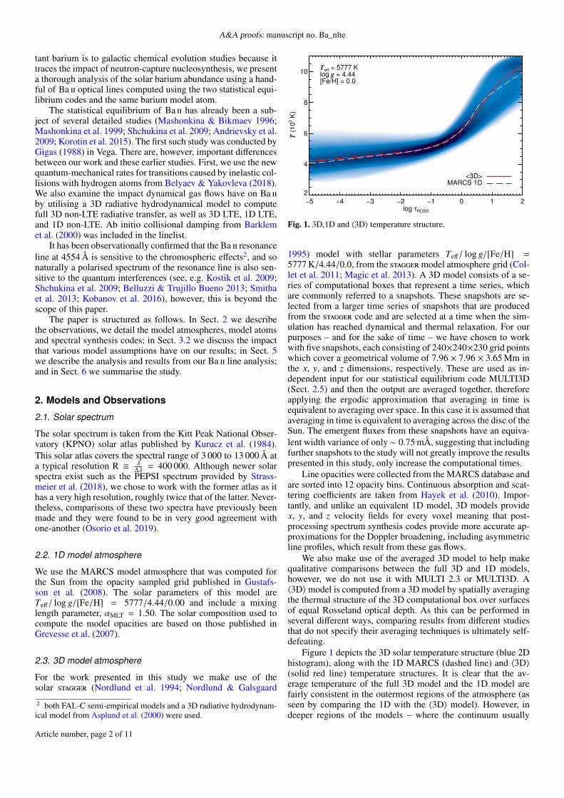
Fig. 1. 3D,1D and 〈3D〉 temperature structure.

1995) model with stellar parameters Teff/ log g/[Fe/H] =5777 K/4.44/0.0, from the staggermodel atmosphere grid (Col-let et al. 2011; Magic et al. 2013). A 3D model consists of a se-ries of computational boxes that represent a time series, whichare commonly referred to a snapshots. These snapshots are se-lected from a larger time series of snapshots that are producedfrom the stagger code and are selected at a time when the sim-ulation has reached dynamical and thermal relaxation. For ourpurposes – and for the sake of time – we have chosen to workwith five snapshots, each consisting of 240×240×230 grid pointswhich cover a geometrical volume of 7.96 × 7.96 × 3.65 Mm inthe x, y, and z dimensions, respectively. These are used as in-dependent input for our statistical equilibrium code MULTI3D(Sect. 2.5) and then the output are averaged together, thereforeapplying the ergodic approximation that averaging in time isequivalent to averaging over space. In this case it is assumed thataveraging in time is equivalent to averaging across the disc of theSun. The emergent fluxes from these snapshots have an equiva-lent width variance of only ∼ 0.75 mÅ, suggesting that includingfurther snapshots to the study will not greatly improve the resultspresented in this study, only increase the computational times.

Line opacities were collected from the MARCS database andare sorted into 12 opacity bins. Continuous absorption and scat-tering coefficients are taken from Hayek et al. (2010). Impor-tantly, and unlike an equivalent 1D model, 3D models providex, y, and z velocity fields for every voxel meaning that post-processing spectrum synthesis codes provide more accurate ap-proximations for the Doppler broadening, including asymmetricline profiles, which result from these gas flows.

We also make use of the averaged 3D model to help makequalitative comparisons between the full 3D and 1D models,however, we do not use it with MULTI 2.3 or MULTI3D. A〈3D〉model is computed from a 3D model by spatially averagingthe thermal structure of the 3D computational box over surfacesof equal Rosseland optical depth. As this can be performed inseveral different ways, comparing results from different studiesthat do not specify their averaging techniques is ultimately self-defeating.

Figure 1 depicts the 3D solar temperature structure (blue 2Dhistogram), along with the 1D MARCS (dashed line) and 〈3D〉(solid red line) temperature structures. It is clear that the av-erage temperature of the full 3D model and the 1D model arefairly consistent in the outermost regions of the atmosphere (asseen by comparing the 1D with the 〈3D〉 model). However, indeeper regions of the models – where the continuum usually


A. J. Gallagher et al.: 3D non-LTE Ba in the Sun

forms (log τROSS ≈ 0) – the models begin to diverge. This ismostly due to the differences between the convection indicativein the 3D hydrodynamic model atmosphere – which the 〈3D〉model traces – and the treatment of convection theory (in thiscase the mixing length theory) in the 1D model atmosphere.

2.4. MULTI 2.3

MULTI solves the equations of radiative transfer and statisticalequilibrium in 1D geometry with 1D model atmospheres. Thelatest release of MULTI is MULTI 2.3. However, we have madeseveral minor changes to MULTI 2.3 for our purposes includ-ing, the ability to compute the detailed balance for charge trans-fer processes between ions and hydrogen. We include a fixedmicroturbulence value of 1 km s−1 in our computations with thesolar MARCS model. The flux data were computed using fiveµ-angles, assuming a Gaussian quadrature scheme taken fromLowan et al. (1942).

2.5. MULTI3D

MULTI3D is an message passing interface (MPI)-parallelised,domain-decomposed 3D non-LTE radiative transfer code thatsolves the equations of radiative transfer using the Multi-levelAccelerated Lambda Iteration (ALI) method (Rybicki & Hum-mer 1991, 1992) for 3D model atmospheres. Every element thatis modelled by MULTI3D is assumed to have no effect on themodel atmosphere, as it is in MULTI 2.3. This is a good assump-tion for barium as it is not an electron donor nor does it have ahigh impact on the overall opacity, unlike magnesium or iron,for example.

At present, it will accept three types of 3D model atmo-spheres formats as direct input, including those computed usingBifrost (Gudiksen et al. 2011), and stagger. While Bifrost mod-els are read using MPI IO, the stagger models are, at present,not read this way due to complications in converting byte order-ing. However, the added delay to the code’s run time is minimal,and only becomes noticeable when MULTI3D is run on severalhundred CPUs. In addition to these two types of model atmo-sphere, the code will also accept any 3D model formatted so thatthe temperature, T , density, ρ, electron number density, ne, andx, y, and z velocity fields are supplied on a Cartesian grid that isboth horizontally periodic and equidistantly spaced. Therefore,it is relatively straightforward to convert almost any 3D modelto this input format for MULTI3D.

We have introduced new coding for computing fluxes insideMULTI3D along with the appropriate post-processing routinesdesigned to extract the flux data. All of the output flux data com-puted for the work presented here was calculated using a Lobattoquadrature scheme and the appropriate corresponding weights(Abramowitz & Stegun 1972). At a later stage of this paper se-ries, other quadrature schemes will be introduced, as well as in-ternal routines that will compute fluxes inside MULTI3D andwrite them as output.

MULTI3D is now capable of accepting model atoms that in-clude hyperfine structure (HFS) and isotope shift information forany atomic transition. This means that lines with highly asym-metric profiles, caused by these effects, can now be adequatelymodelled by MULTI3D. To test this upgrade, and to test that wecould limit the impact of systematic errors dominating the abun-dances and abundance corrections we provide, we compared 1Dspectra computed by both MULTI 2.3 and MULTI3D. This wasconducted only for the vertical intensity (µ = 1), using a small

test barium model atom, under the assumption of LTE. We usethe same opacity sources, and same input model atmosphere.Systematic differences in the equivalent widths of less than2.2 % were found between intensities computed with MULTI2.3 and intensities computed with MULTI3D. This translatesto abundances differences much less than 0.01 dex. The reasonfor these small differences is likely because of the way eachcode solves the radiative transfer equation; MULTI3D uses a di-rect 1D integration of the radiative transfer equation when com-puting spectra from 1D model atmospheres3, while MULTI 2.3utilises a faster Feautrier method. However, abundance uncer-tainties found here are far smaller than the errors we report inSect. 5. Therefore, we were satisfied that comparing 1D outputfrom MULTI 2.3 with 3D output from MULTI3D was adequate.

We ran MULTI3D in short characteristic 3D solver mode andused the solar stagger model as input. The stagger model’s xygrid points were scaled down by a factor of 64 from 240×240 to30× 30 grid points using a simple bilinear interpolation scheme.Significant tests conducted in the first paper in this paper series,(Bergemann et al. 2019, henceforth, Paper I), revealed no signif-icant loss of information in the horizontal gas flows that affectedthe line profiles in any noteworthy way. The horizontal compo-nents were also assumed to be periodic so that rays with very lowµ angles could be computed without encountering a horizontalboundaries. The vertical grid size remained consistent with theoriginal model atmosphere at 230 grid points.

2.6. Model of Barium atom

The model atom of barium is constructed as follows. The en-ergy levels for the Ba i and Ba ii levels are extracted from theNIST database. Of these, we include eight energy states of Ba iup to the energy of 2.86 eV, and all available levels of Ba ii upto 9.98 eV. Fine structure is retained for the three lowest termsof Ba ii: 6s 2S (ground state), 5d 2D (∼ 0.65 eV), and 6p 2P◦(∼ 2.6 eV) (Table 1). Transitions between these terms are typ-ically used in the barium abundance analysis of cool stars. Otherlevels are merged into terms, and their energy levels are rep-resented by the weighted sum of the individual components(weighted by the statistical weights of the levels). In total, themodel is comprised of 110 states and is restricted by the groundstate of Ba iii at 15.2 eV for a total of 111 levels. Note that nolines of Ba i are observed in the spectra of FGK stars. For theSun nBa i/nBa ii ≈ 10−4 − 10−6 (see Sect. 3.1), hence, Ba i is a mi-nority species. As such, a detailed treatment of the neutral stageis of no importance to the statistical equilibrium Ba ii, which isthe majority species in these stars. Figure 2 depicts the energylevels in Ba ii and transitions among them in the form of a Gro-trian diagram. We have colour-coded the four lines we use hereas follows: gold represents the Ba ii 4554 Å line; green repre-sents the 5853 Å line; blue represents the 6141 Å line; and redrepresents the 6496 Å line. As there are too many energy levelsin the model atom to accurately depict without overlapping en-ergy states, this figure should be used for qualitative assessmentsonly.

The radiative bound-bound transitions for Ba ii were ex-tracted from the Kurucz database, 26.03.2017. We also com-pared the data with the NIST database. For the combinedterms, the lines were merged and the transition probabilities co-added as described in Bergemann et al. (2012a). The oscillatorstrengths of the four diagnostic lines used for the present analy-

3 ordinarily MULTI3D uses a short-characteristic solver for 3D modelatmospheres.


http://kurucz.harvard.edu/atoms/5601/gf5601.all

https://physics.nist.gov/PhysRefData/ASD/lines_form.html


Table 1. The Ba ii lines used in the abundance analysis of the Sun

Wavelength [Å] Elow (eV) Eup (eV) conf conf log g f VdW EW (mÅ)

4554.033 0.00 2.72 6s 2S0.5 6p 2P◦1.5 0.170 ± 0.004 303.222 2075853.675 0.60 2.72 5d 2D1.5 6p 2P◦1.5 −1.023 ± 0.005 365.264 686141.713 0.70 2.72 5d 2D2.5 6p 2P◦1.5 −0.070 ± 0.005 365.264 1266496.898 0.60 2.51 5d 2D1.5 6p 2P◦0.5 −0.365 ± 0.004 365.264 102

Notes. The wavelengths are given in air. The equivalent widths correspond to the measurements in the solar KPNO flux atlas and are given inmÅ. The Van der Waals broadening parameters are taken from Barklem et al. (2000). The log g f values reported here are derived from the veryaccurate transition probabilities taken from De Munshi et al. (2015) and Dutta et al. (2016).

Fig. 2. The Grotrian diagram of Ba ii atom. Gold, green, blue, and redlines indicate the diagnostic Ba ii lines that we use in the solar abun-dance analysis at 4554, 5853, 6141, 6496 Å, respectively.

sis were extracted from the experimental transition probabilitiespresented in De Munshi et al. (2015) and Dutta et al. (2016).In total, the model contains 284 spectral lines in the wavelengthrange from 1330 to 202930 Å. The transitions with log g f < −10are not included. Most of these lines are represented by nine fre-quency points, except for the four diagnostic lines that we use inthe abundance analysis, i.e the lines at 4554, 5853, 6141, and6496 Å. These lines were represented with a profile contain-ing 301 frequency points. Several UV lines are rather strong.To test whether nine frequencies were enough to describe thosestrong lines, we ran a test using MULTI 2.3. The departure coef-ficients from the model atom were compared with an atom thatcontained 100 frequency points for two strong UV transitions at2304.247 Å and 2341.429 Å. It was found that these transitionshave no effect on the populations of the four barium lines of in-terest. This justifies the number of frequency points chosen fortransitions that were not of interest to us for this study. Dampingby elastic collisions with hydrogen atoms are computed usingthe α and σ parameters from Barklem et al. (2000) where avail-able. When this information was missing, we used the Unsöldapproximation, which was scaled by 1.5. The wavelengths aretaken from Karlsson & Litzén (1999). We found that for threelines (NB: not the line at 4554 Å) there was a systematic off-set to the solar spectrum. Once the solar spectrum was correctedfor gravitational redshift they did match the observed line posi-tions, although the 4554 Å resonance line has a slightly differentshift. Karlsson & Litzén underline that this line might be slightly

shifted in their measurements, due to the isotopic mix they usedand self-absorption in this strong line. This shift is however ex-pected to be at most 1 mÅ to the blue (Litzén, private comm.) notsufficient to explain the remaining offset we observe. We discov-ered that the excess shift in this line was due to convective ef-fects. We shifted the 4554 Å line by 2 mÅ in 1D to the blue tomatch the observed position, whereas we did not need to shiftthe 3D profile.

We also introduce HFS and isotopic shifts. They were com-puted using the solar abundance ratios of the five barium iso-topes, see Eugster et al. (1969). The odd barium isotopes havenon-zero nuclear spins that causes hyperfine splitting of the lev-els. The magnetic dipole and electric quadrupole constants forthe five relevant energy levels were taken from Silverans et al.(1986), and Villemoes et al. (1993). The isotopic shifts are pro-vided by van Hove (1982) for the 5853 and 6141 Å lines, byVillemoes et al. (1993) for the 6496 Å line, and by Wendt et al.(1984) for the 4554 Å line. The diagnostic lines are hence rep-resented by six to 15 HFS components. The complete HFS in-formation for these lines can be found in tables in Appendix A.Oscillator strengths for these lines are computed from accurateexperimental transition probabilities in De Munshi et al. (2015)Dutta et al. (2016).

The radiative bound-free data are computed using the stan-dard hydrogenic approximation (Kramer’s formula). This is ap-propriate since the first ionisation potential of Ba ii is at 10 eV,and the energy levels, which may contribute to radiative over-ionisation at the solar flux maximum, have very low popula-tion numbers. Also on the basis of earlier studies with strontium(Bergemann et al. 2012b), which has a similar atomic structure,we do not expect that photo-ionisation is a significant non-LTEeffect. In fact, earlier studies of barium in non-LTE showed thatBa ii a majority ion and is collision-dominated (see Mashonk-ina et al. 1999; Gehren et al. 2001; Bergemann & Nordlander2014). In such ions, the statistical equilibrium is established by acompetition of collisional thermalisation, photon losses in stronglines, and over-recombination. This will be discussed in detail inthe next section.

One of the new features of our atom, compared to earlierstudies mentioned above, is the treatment of collisions. In par-ticular, we include the new quantum-mechanical rate coefficientsfor the inelastic collisions between the Ba ii ions and hydrogenatoms by Belyaev & Yakovleva (2017, 2018). To the best of ourknowledge, the first study of barium that employs these detailedquantum-mechanical data for collisions with hydrogen was re-cently published by Mashonkina & Belyaev (2019) for the pur-poses of treating isotopes. The present paper is the first timethese hydrogen-collision data have been employed for full non-



LTE modelling. The data are available for 686 processes, andrepresent collisional excitation and charge transfer reactions, i.e.Ba + H ↔ Ba+ + H−. The rate coefficients are typically largeand may exceed 10−8 cm3s−1 in the temperature regime relevantto modelling the solar atmosphere. Note that here the processionisation refers to the ion we are interested in and a free elec-tron, i.e. ionisation: Ba ii + H → Ba iii + H + e, but the procession-pair formation reads: Ba ii + H → Ba iii + H−, that is, Ba iiloses its outer electron and it is bound with H. Its inverse process,mutual neutralisation, is the process when Ba iii gains an electronfrom H−. The same is valid when Ba ii is replaced by Ba i andBa iii is replaced by Ba ii. Charge transfer reactions do not leadto a free electron, which is the case that is usually modelled bya Drawin’s formula (Drawin 1968, 1969). Excitation and ionisa-tion by collisions with free electrons are computed using the vanRegemorter (1962) and Seaton (1962) formulae. A study of theimpact of different collisional rates was presented in Andrievskyet al. (2009, Sect. 3.2). No differences between these classicalrecipes were found. An earlier version of this model atom wasused in (Eitner et al. 2019). We have since updated the oscillatorstrengths.

3. Barium line formation

3.1. non-LTE effects

In terms of departures from LTE, Ba ii is a collision-dominatedion (see Gehren et al. 2001, and references therein). The ioni-sation potential is too high for photo-ionisation to play a signif-icant role in the statistical equilibrium (SE) in FGK type stars.On the other hand, the term structure of the ion, with severalvery strong radiative transitions, favours strong effects causedby line scattering. In particular, there is radiative pumping atthe frequencies of optically-thin line wings, τwing < 1, as longas at the line centre τcore > 1. This mechanism acts predomi-nantly at larger depths and leads to over-population of the up-per levels of the transitions, at the expense of the lower states.On the other hand, strong downward cascades occur higher upin the atmosphere, where the strong line cores become opticallythin, τcore < 1. This mechanism de-populates the upper levelsvia spontaneous de-excitations and this downward electron cas-cade causes over-population of the lower-lying energy states. Asthe statistical equilibrium of Ba ii has been extensively studied inthe literature (Mashonkina & Bikmaev 1996; Mashonkina et al.1999; Short & Hauschildt 2006; Mashonkina et al. 2008), hencein what follows we will only describe the main features of thenon-LTE line formation and discuss the differences with the ear-lier studies.

Quantitatively, this behaviour can be visualised as plots ofthe departure coefficients bi

4 as a function of the continuum op-tical depth at 5000 Å, log τ5000. Figure 3 depicts the bi behaviourfor the solar MARCS model atmosphere. To facilitate the com-parison with the detailed study by Mashonkina et al. (1999), wehave chosen the same axis range as that paper. Thick colouredcurves correspond to 5 energy states, which are involved in theradiative transitions listed in Table 1: the ground state of Ba ii,6s 2S, and the low-excitation terms 5d 2D and 6p 2P◦. Thin greydotted curves show all other energy levels of Ba ii in the modelatom. It is interesting that despite major differences in the modeland numerical methods, including the properties of the atomic

4 The departure coefficient is defined as the ratio of atomic numberdensity for a given energy level i computed in non-LTE to that of LTE,bi =

ni,non−LTEni,LTE

.

−5 −4 −3 −2 −1 0 1log τ5000

0.4

0.6

0.8

1.0

1.2

1.4

bi

6s 2S

6p 2P

5d 2D

Ba III

Fig. 3. Departure coefficients for the Ba ii levels as a function of thecontinuum optical depth log τ5000 computed using the reference bariummodel atom for the solar MARCS model atmosphere.

model, model atmosphere, and the SE code, the agreement be-tween our results and that of Mashonkina et al. (1999, see theirFig. 2) is very good. In particular, the Ba ii ground state is en-tirely thermalised throughout the full optical depth range and de-velops a very modest over-population only at log τ5000 < −4. Thefirst excited metastable state 5d 2D is also close to LTE due tostrong collisional coupling with the Ba ii ground state, althoughminor departures in the atomic number densities, of the order ofa few percent, are seen at log τ5000 < −3 and higher up. The term6p 2P◦ at ∼ 2.6 eV shows stronger deviations from LTE alreadyin the deep layers, log τ5000 ∼ −2, where the non-LTE populationof the level is only about 80% of the LTE value (that is equivalentto bi = 0.8). The pronounced depletion of the term is caused byphoton losses in the lines, connecting the ground state and thelowest metastable state with 6p 2P◦. This under-population in-creases outwards as the lines become optically thin. All energylevels above 6p 2P◦ are over-populated at log τ5000 < 0, the effectthat Mashonkina et al. (1999) attributed to radiative pumping.

It is interesting to briefly discuss the importance of micro-physical processes in the SE of Ba ii. Andrievsky et al. (2009)suggest that photo-ionisation cross-sections is the main sourceof uncertainty in the SE of Ba ii. This is only true for Ba i, how-ever, no lines of the neutral atom are observed in the opticalor infra-red spectra of FGKM stars (Tandberg-Hanssen 1964).Over-ionisation of Ba i has no effect on the population of Ba ii,as the ratios of number densities of two ionisation stages arenBaI/nBaII ∼ 10−4 at log τ5000 ≈ 0, and drops to ∼ 10−6 inthe outermost atmospheric layers in the solar model. This ratiois even more extreme in the atmospheres of metal-poor stars.For example, for a model atmosphere of an RGB star withTeff = 4600 K, log g = 1.6, and [Fe/H] = −2.5, nBaI/nBaII ∼ 10−5

at log τ5000 ≈ 0, but approaches ∼ 10−10 close to the outer bound-ary at log τ5000 ≈ −5. On the other hand, photoionisation in Ba iiis not important. The ion has a very high ionisation potential,and its well-populated energy levels with low excitation poten-tials have ionisation thresholds in the far-UV, at λ < 1000 Å,where radiative flux in FGK-type stars is negligibly small. Wealso recomputed the departure coefficients assuming σphoto/100and σphoto × 100. This is a very conservative estimate of uncer-tainty in the cross-sections, when comparing to a very similaratom, Sr, for which detailed quantum-mechanical cross-sectionsare available from (Bergemann et al. 2012a). It was found that



only the non-LTE populations of the Ba iii ground state change,but none of the important Ba ii levels show any difference withrespect to our reference model.

A more important ingredient for the SE of Ba ii seems to bethe accuracy of the data for inelastic collisional processes, in par-ticular, those between Ba ii and H i atoms. Short & Hauschildt(2006) suggest that the non-LTE line profiles are invariant toa factors of 0.1 − 10 changes in the rates of transitions causedby collisions (NB they used approximate analytical formulae torepresent these data). This may hold for a limited range of stel-lar parameters. For example, in the case of the Sun, using theDrawin’s recipe or QM data does not give significantly differentresults. However, it is known that metal-poor stars are sensitiveto non-LTE effects (Bergemann & Nordlander 2014). Therefore,it would be reasonable to assume that they would also be sen-sitive to different collisional recipes. This is particularly true inhydrodynamic model atmospheres as the decoupled non-localradiation field leads to a cooling in the outer regions of the tem-perature structure, relative to the equivalent 1D model (see e.g.Gallagher et al. 2016, their Fig. 1). We intend to explore this inthe near future.

3.2. Line formation in hydrostatic and inhomogeneousmodels

We begin with the analysis of LTE and non-LTE formation ofBa ii lines in the 1D hydrostatic solar model. We will then ex-tend the analysis to radiative transfer with 3D inhomogeneousmodels.

As discussed in the previous section, the non-LTE effects inBa ii are primarily dominated by line scattering. Consequently,deviations from LTE in the line source function are expected tobe significant. Since the ratio of the departure coefficients for thelower i and upper j level of the transitions is below unity for thediagnostic Ba ii lines, b j/bi < 1, the ratio of source function tothe Planck function (see Bergemann & Nordlander 2014, for thederivation), also drops below unity. In other words, the sourcefunction in the line is sub-Planckian and the non-LTE lines pro-files shall come out stronger than the LTE lines. In some cases(e.g. Bergemann et al. 2012a, for Sr), this effect is modulated bythe change of the line opacity. However, since κν ∼ bi, and thepopulation numbers for the lower levels of all Ba ii lines are es-sentially thermal throughout the line formation depths, the lineopacity is very close to its LTE value. This simple analytical pic-ture is confirmed by comparing the LTE and non-LTE line pro-files (Fig. 4). The non-LTE effects are small and amount to theabundance difference of −0.05 (4554 Å) to −0.1 dex (5853Å).The other two Ba ii lines show similar behaviour.

Figure 4 demonstrates that the 3D profiles are asymmetricand also shifted blueward relative to the 1D profiles, which isexpected. This is a natural result of the convective motions in-side the 3D model, that the 1D model cannot replicate (Löhner-Böttcher et al. 2018; Stief et al. 2019). This is particularly ob-vious in the three subordinate lines, where the HFS has far lessimpact to the line shape than it does in the resonance line, whereasymmetries are seen in both 1D and 3D. The 3D profiles, fora given barium abundance, are consistently weaker than their1D counterparts, both in LTE and non-LTE. Therefore, positiveabundance corrections are going to be needed to reproduce thesame equivalent width, foreshadowing larger 3D LTE and non-LTE abundances over the 1D LTE counterpart. Like was shownin the hydrostatic case above, deviations from LTE should besignificant because of line scattering.

Table 2. 1D non-LTE, 3D LTE, and 3D non-LTE (NLTE) abundancecorrections, ∆.

Wavelength (Å) ∆1D NLTE ∆3D LTE ∆3D NLTE

4554.033 −0.05 0.11 0.085853.673 −0.11 0.05 0.036141.711 −0.15 0.10 0.046496.896 −0.19 0.10 0.02

Notes. Corrections are defined as ∆D = A(X)D − A(X)1D LTE, where D isthe 3D non-LTE, 3D LTE, or 1D non-LTE case.

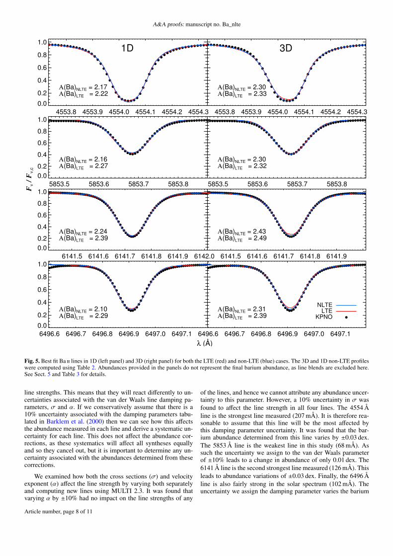
The lines of Ba ii in the solar spectrum are strong, with EW’sfrom 207 mÅ (4554 line) to 68 mÅ (5853 Å) line. As such, theyare not only extremely affected by damping, but are also blended.The 4554 Å line is blended by a Fe ii feature close the line core,but has little impact on the line. The subordinate lines also showsome blending. Korotin et al. (2015) avoided, in particular, the4554 Å line in their analysis of FGK metal-poor stars in starswhere [Fe/H] > −1.0. On the other hand, Grevesse et al. (2015)included the 4554, 5853, and 6496 Å line in their analysis of theSun. They also used the non-LTE corrections for Ba ii lines. Weexplore the effects of line blending and damping in Sect. 5.

The current photospheric solar abundance of barium derivedby Grevesse et al. (2015) – who applied non-LTE correctionsto their 3D LTE abundance – is 2.25 ± 0.03 ± 0.07 (where er-rors represent the statistical and systematic errors, respectively).The abundance of barium in CI meteorites (Lodders 2003) is2.19 ± 0.03. The main goal of this paper is to explore whetherab initio atomic data from physical experiments and detailedquantum-mechanical calculations are successfully able to de-scribe the spectrum of the Sun. Accordingly, we now move onto report our 1D non-LTE, 3D LTE and 3D non-LTE correctionsrelative to the average barium 1D LTE abundance.

4. Computing abundance corrections

A grid of abundances for all four barium lines were computedusing MULTI 2.3. These were fit to the solar spectrum using aχ2 code that treats abundances, macroturbulent broadening andwavelength shifts as free parameters (see Sect. 2.6 for detailsof line shifts). The macroturbulences found ranged from 1.5 −1.9 km s−1. The code also normalises the fit to a local continuumfor each line using two patches of spectrum either side of theline. We fixed the rotational broadening to v sin i = 1.6 km s−1

(Pavlenko et al. 2012). The 1D LTE we attain represent the beststatistical fit from this χ2 code.

We computed the four barium lines in 1D non-LTE, 3D LTEand 3D non-LTE using three abundances; A(Ba) = 2.17, 2.27and 2.35 - covering typical abundances reported in the litera-ture for the solar barium abundance. The abundance correctionstabulated in Table 2 were determined by fitting the grid of 1DLTE profiles to the 1D non-LTE, 3D LTE and non-LTE linesso that their equivalent widths matched. Unsurprisingly, it wasfound that the corrections from all three abundances were iden-tical, hence corrections we provide are robust against the typi-cal abundance range found by most studies on the solar bariumabundance.



0.0

0.2

0.4

0.6

0.8

1.0 4554 Å

5853 Å

−0.2 −0.1 0.0 0.1 0.20.0

0.2

0.4

0.6

0.8

1.0 6141 Å

−0.2 −0.1 0.0 0.1 0.2

6496 Å

LTENLTE

3D1D

Fν /

Fν

,c

∆λ (Å)

Fig. 4. 1D (black) and 3D (blue) LTE (dashed-lines) and non-LTE (solid-lines) Ba ii line profiles at A(Ba) = 2.26 dex. No extra broadening wasadded to any of the depicted lines. The 3D profiles are shown to be shifted relative to the 1D profiles. This is a natural consequence of the convectiveshifts indicative to a dynamic model atmosphere.

5. Results

Our best fit profiles are compared with the solar flux profiles inFig. 5. The best fit 3D lines are computed by MULTI3D usingthe corrections given in Table 2. The 3D non-LTE abundancesare remarkably consistent, apart from the 6141 Å line, which isapproximately 0.12 dex larger than the other three. The reasonsfor this will become apparent by the end of this section. Unlikein the 1D case, the best fit 3D LTE profiles show large deviationsin the line cores, relative to their non-LTE counterparts, yet theirequivalent widths remain very similar.

The lines and abundances discussed this far have assumedthat the barium lines are unblended in the solar spectrum. In re-ality this is not the case. In fact, the abundances all barium lines(particularly the 6141 Å line) are dependent on line blending, aswe now discuss.

5.1. Line blending corrections

The four barium lines we model here suffer from the effects ofblending with other atomic and molecular species. Naturally, thisimpacts the abundances we derive when we assume that the lineis clean. This is what was done when synthesising the lines withMULTI3D and MULTI 2.3, as these codes do not currently pos-sess the capability to synthesise blends. To examine this, we usedthe VALD35 database together with the barium line informationextracted from the model atom to create new line lists for the

5 http://vald.astro.uu.se/

1D LTE spectrum synthesis code, MOOG6. This code was cho-sen as the interactive plotting tool makes recomputing syntheticspectra and fitting it with observed data very simple. Lines werecomputed with and without and the abundance of the clean bar-ium line was adjusted until its line strength matched the blendedline.

The Ba ii resonance line at 4554 Å is the strongest line pre-sented here. Naturally, it would dominate most of the line de-pression at this spectral region. It is found that when blends areincluded, the 1D LTE barium abundance must be reduced by0.01 dex. The 5853 Å line abundance was reduced by 0.03 dex.The 6141 Å line was found to be severally affected by blending,as the abundance had to be reduced by 0.16 dex. The 6496 Å bar-ium abundance had to be reduced by 0.04 dex.

We will use these abundance corrections to determine thebarium abundance in all four paradigms in Sect. 5.4. First, how-ever, it is important to determine how the barium lines are af-fected by systematic uncertainties, as we now present.

5.2. Line damping uncertainties

We have previously mentioned that differences in the radiativetransfer solvers used by MULTI 2.3 and MULTI3D lead to ex-tremely small systematic uncertainties in the barium abundance.These are small (< 0.01 dex) enough to be dwarfed by uncertain-ties associated with the van der Waals broadening parameters,now discussed. The barium lines synthesised here have varying

6 https://www.as.utexas.edu/~chris/moog.html


http://vald.astro.uu.se/

https://www.as.utexas.edu/~chris/moog.html


4553.8 4553.9 4554.0 4554.1 4554.2 4554.30.0

0.2

0.4

0.6

0.8

1.0

Α(Ba)LTE = 2.22Α(Ba)NLTE = 2.17

4553.8 4553.9 4554.0 4554.1 4554.2 4554.3


5853.5 5853.6 5853.7 5853.80.00.2

0.4

0.6

0.8

1.0


5853.5 5853.6 5853.7 5853.8


6141.5 6141.6 6141.7 6141.8 6141.9 6142.00.00.2

0.4

0.6

0.8

1.0


6141.5 6141.6 6141.7 6141.8 6141.9


6496.6 6496.7 6496.8 6496.9 6497.0 6497.10.0

0.2

0.4

0.6

0.8

1.0


6496.6 6496.7 6496.8 6496.9 6497.0 6497.1


KPNOLTE

NLTE

Fν /

Fν

,c

λ (Å)

1D 3D

Fig. 5. Best fit Ba ii lines in 1D (left panel) and 3D (right panel) for both the LTE (red) and non-LTE (blue) cases. The 3D and 1D non-LTE profileswere computed using Table 2. Abundances provided in the panels do not represent the final barium abundance, as line blends are excluded here.See Sect. 5 and Table 3 for details.

line strengths. This means that they will react differently to un-certainties associated with the van der Waals line damping pa-rameters, σ and α. If we conservatively assume that there is a10% uncertainty associated with the damping parameters tabu-lated in Barklem et al. (2000) then we can see how this affectsthe abundance measured in each line and derive a systematic un-certainty for each line. This does not affect the abundance cor-rections, as these systematics will affect all syntheses equallyand so they cancel out, but it is important to determine any un-certainty associated with the abundances determined from thesecorrections.

We examined how both the cross sections (σ) and velocityexponent (α) affect the line strength by varying both separatelyand computing new lines using MULTI 2.3. It was found thatvarying α by ±10% had no impact on the line strengths of any

of the lines, and hence we cannot attribute any abundance uncer-tainty to this parameter. However, a 10% uncertainty in σ wasfound to affect the line strength in all four lines. The 4554 Åline is the strongest line measured (207 mÅ). It is therefore rea-sonable to assume that this line will be the most affected bythis damping parameter uncertainty. It was found that the bar-ium abundance determined from this line varies by ±0.03 dex.The 5853 Å line is the weakest line in this study (68 mÅ). Assuch the uncertainty we assign to the van der Waals parameterof ±10% leads to a change in abundance of only 0.01 dex. The6141 Å line is the second strongest line measured (126 mÅ). Thisleads to abundance variations of ±0.03 dex. Finally, the 6496 Åline is also fairly strong in the solar spectrum (102 mÅ). Theuncertainty we assign the damping parameter varies the barium



abundance found in this line by ±0.02 dex. The list of associatedabundance uncertainties can be seen in column four of Table 3.

Uncertainties in line blends are also of concern when com-puting abundances. No uncertainty information is given byVALD, so we again conservatively assume that the log g f val-ues of these lines have a 10% uncertainty. The abundances at-tained from the 4554 Å line with and without line blending werevirtually identical. As previously mentioned, this is because theresonance line dominates line depression around this spectral re-gion. Accordingly, uncertainties in blended lines of ±10% donot affect the barium abundance. While the 5853 Å line is theweakest line analysed, it suffers the least from blending. As such,there is also no sensitivity in barium abundance found from vary-ing the blended lines. The blends around the 6141 Å line have alarge impact on the barium abundance. Naturally, uncertaintiesin log g f lead to an uncertainty of ±0.02 dex. Therefore, the in-clusion of blend uncertainties increases systematic uncertaintyof the 6141 Å from 0.03 dex to 0.04 dex. Finally, the blendinguncertainties around the 6496 Å line were not found to influencethe barium abundance. A break down of the associated abun-dance uncertainties can be seen in column five of Table 3.

5.3. Oscillator strength uncertainties

The oscillator strengths ( f -values) of the four diagnostic linesused in the present study are taken from De Munshi et al. (2015)and Dutta et al. (2016). They also provide unique errors associ-ated to each transition probability, which we convert in to oscil-lator strength uncertainties. The transition probabilities are ex-tremely accurate, so the resulting uncertainties are very small.When these are included in our calculations we find that thepropagated abundance error associated with the 4554 Å line is±0.00 dex. The weakest line in our sample (5853 Å) has a prop-agated abundance uncertainty of ±0.01 dex. The most blendedline (6141 Å) is found to have a propagated abundance uncer-tainty of ±0.01 dex. Finally, the 6496 Å line has an associatedabundance error of ±0.01. The associated abundance uncertain-ties for each line can be found in column six of Table 3.

5.4. Solar barium abundance

We now present the barium abundance in four paradigms: 3Dnon-LTE, 3D LTE, 1D non-LTE and 1D LTE. We correct the 1DLTE abundances using the corrections in Table 2 and Sect. 5.1,and weight them by their uncertainties listed in Table 3 using aninverse-variance weighted mean (

∑ωi Xi, where ωi = 1

σ2 ).We report for the first time a full 3D non-LTE solar barium

abundance of 2.27 ± 0.02 ± 0.01, where errors given here arethe systematic uncertainties and the random error determined asthe standard deviation found in the line-to-line scatter of the 3Dnon-LTE abundances, which can also be seen in Table 3. Thisvalue is 0.08 dex larger than the meteoritic barium abundance of2.19 ± 0.03 determined by Lodders (2003). We therefore find aphotospheric abundance that is slightly larger than that reportedfrom meteorites.

Using the same method just described, we find that A(Ba) =2.31±0.02±0.03 in 3D LTE. Errors again represent the system-atic and random errors, like above. When we use 1D model at-mospheres and apply non-LTE physics to the post-process spec-tral synthesis we find that the 1D non-LTE barium abundanceis A(Ba) = 2.11 ± 0.02 ± 0.05. Finally, when we derive the bar-ium abundance using the classical 1D LTE approach we find that

A(Ba) = 2.24 ± 0.02 ± 0.02. This abundance is similar to the 3Dnon-LTE abundance.

6. Conclusions

We have computed new values of the solar barium abundancebased upon results computed using a new barium model atomthat includes quantum mechanical inelastic collisional rate co-efficients between Ba ii and hydrogen. We computed the bariumabundance using a static 1D model atmosphere and provide 1Dnon-LTE, 3D LTE and 3D non-LTE corrections to this value inTable 2. Using these corrections we also present new solar photo-spheric barium abundances for the first time in full 3D non-LTE,as well as in 3D LTE, 1D non-LTE and 1D LTE.

The summary of this work is as follows (NB that all abun-dances given below are done so by adding the corrections to each1D LTE abundance and then calculating the inverse-varianceweighted mean as described in Sect. 5.4):

– The 3D non-LTE barium abundance was found to be A(Ba) =2.27 ± 0.02 ± 0.01, which is 4σ larger the meteoritic abun-dance published by Lodders (2003). This may suggest uncer-tainties in the atomic data and/or that further physics is stillmissing from our analyses, such as the treatment of magneticfields. On the other hand, Ba isotopic abundance anomaliesare well-documented in CI meteorites (e.g. McCulloch &Wasserburg 1978; Arnould et al. 2007) and it is not clearwhether the meteoritic value can be indeed directly com-pared to the solar photospheric estimate. Nevertheless, thisvalue represents the best photospheric solar barium abun-dance available from the current state-of-the-art in spectralmodelling. As a result, it provides a remarkably consistentabundance for the four diagnostic lines.

– The 3D LTE abundance was determined as A(Ba) = 2.31 ±0.02 ± 0.03. This value is larger than the meteoritic valuegiven in Lodders and the 3D non-LTE abundance we deter-mine, and the individual abundances are not as consistent.

– The 1D non-LTE abundance of A(Ba) = 2.11 ± 0.02 ± 0.05suggests that the barium abundance is depleted by 0.16 dexin the solar atmosphere relative to the full 3D non-LTE. Theabundance is also smaller than the meteoritic result reportedin Lodders and the inconstencies between lines are largerthan they are in 3D non-LTE.

The 3D non-LTE and 1D LTE abundances are very similarfor barium in the Sun, but larger than that given in Lodders(2003). Conversely, the 3D LTE abundance suggests that bar-ium abundance is even larger in the Sun, while the 1D non-LTEabundance suggests barium is slightly lower than the meteoriticvalue. It is clear then that the inclusion or removal of realistictreatments of line formation physics or convection has opposingeffects on the barium abundance; the former strengthens the bar-ium lines and so depletes the barium abundance, while the latterweakens the barium lines and hence a larger barium abundanceis required. Therefore, the exclusion of both physical processesin the 1D LTE paradigm masks each effect, providing similarvalues in each line as the actual values found in 3D non-LTE.Conversely, in our work on manganese we found that the 3Dand Non-LTE effects do not cancel out, but rather the effects ofNon-LTE are amplified in 3D calculations with hydrodynamicalmodels.

The previous set of transition probabilities reported byDavidson et al. (1992) led to abundances values that were, ingeneral, less consistent than those reported here and had larger



Table 3. Abundances, associated error estimates and abundance corrections due to line blending.

LTE non-LTEWavelength (Å) A(Ba)1D,LTE ∆blend σBPO σblends σ f−value σtotal A(Ba)1D A(Ba)3D A(Ba)1D A(Ba)3D

4554.033 2.22 −0.01 ±0.03 ±0.00 ±0.00 ±0.03 2.21 2.32 2.16 2.295853.673 2.27 −0.03 ±0.01 ±0.00 ±0.01 ±0.01 2.24 2.29 2.13 2.276141.711 2.39 −0.16 ±0.03 ±0.02 ±0.01 ±0.04 2.23 2.33 2.08 2.276496.896 2.29 −0.04 ±0.02 ±0.00 ±0.01 ±0.02 2.25 2.35 2.06 2.27

Notes. Column 2 tabulates the 1D LTE abundances found when the lines were assumed to be clean. They are consistent with the profiles depictedin Fig. 5. Column 3 presents the abundance correction associated with line blending. The final four columns present actual abundances of eachline when the appropriate corrections were added to Cols. 2 and 3 from Table 2. The weighted averages calculated in Sect. 5.4 are computed usingthese abundances and the systematic errors tabulated in Col. 7 from the errors in BPO theory (Barklem et al. 2000), line blend uncertainties, andoscillator strengths, f , which are presented in Cols. 4, 5, and 6, respectively.

uncertainties associated to them, with the 5853 Å line being mostuncertain and most inconsistent with the other three diagnosticlines. The latest published transition probabilities in De Munshiet al. (2015) and Dutta et al. (2016) represent the most accuratetransition parameters published. As such, the barium abundanceswe find from each diagnostic line used here are all in very goodagreement (once the blending corrections are included).

We have presented this work as part of a larger series of pa-pers designed to report on the development of the MULTI3Dspectrum synthesis code. Up until now we have added new cod-ing that allows it to read standard stagger model atmospheres;include the effect of charge transfer between hydrogen and ions;compute flux data based on hard-coded quadrature schemes; andcompute multi-component transitions caused by HFS or isotopesplittings. Further physics and mathematical techniques will beadded as the project progresses that will be presented in futurepapers in this paper series. We also plan to extend our work onbarium within this paper series to include several metal-poorbenchmark stars, where the present work will be important tothe relative abundances we report.Acknowledgements. This work made heavy use of the Max Planck Computing& Data Facility (MPCDF) for the majority of the computations. This projectwas funded in part by Sonderforschungsbereich SFB 881 "The Milky WaySystem" (subproject A5) of the German Research Foundation (DFG) and bythe Research Council of Norway through its Centres of Excellence scheme,project number 262622. SAY and AKB gratefully acknowledge support fromthe Ministry for Education and Science (Russian Federation), project Nos.3.5042.2017/6.7, 3.1738.2017/4.6. BP is partially supported by the CNES, Cen-tre National d’Etudes Spatiales.

ReferencesAbramowitz, M. & Stegun, I. A. 1972, Handbook of Mathematical FunctionsAmarsi, A. M. & Asplund, M. 2017, MNRAS, 464, 264Amarsi, A. M., Asplund, M., Collet, R., & Leenaarts, J. 2016, MNRAS, 455,

3735Andrievsky, S. M., Spite, M., Korotin, S. A., et al. 2009, A&A, 494, 1083Arlandini, C., Käppeler, F., Wisshak, K., et al. 1999, ApJ, 525, 886Arnould, M., Goriely, S., & Takahashi, K. 2007, Phys. Rep., 450, 97Asplund, M., Carlsson, M., & Botnen, A. V. 2003, A&A, 399, L31Asplund, M., Nordlund, Å., Trampedach, R., Allende Prieto, C., & Stein, R. F.

2000, A&A, 359, 729Barklem, P. S., Piskunov, N., & O’Mara, B. J. 2000, A&AS, 142, 467Belluzzi, L. & Trujillo Bueno, J. 2013, ApJ, 774, L28Belyaev, A. K. & Yakovleva, S. A. 2017, A&A, 608, A33Belyaev, A. K. & Yakovleva, S. A. 2018, MNRAS, 478, 3952Bergemann, M., Gallagher, A. J., Eitner, P., et al. 2019, arXiv e-prints

[arXiv:1905.05200]Bergemann, M., Hansen, C. J., Bautista, M., & Ruchti, G. 2012a, A&A, 546,

A90Bergemann, M., Lind, K., Collet, R., Magic, Z., & Asplund, M. 2012b, MNRAS,

427, 27

Bergemann, M. & Nordlander, T. 2014, arXiv e-prints [arXiv:1403.3088]Carlsson, M. 1986, Uppsala Astronomical Observatory Reports, 33Collet, R., Magic, Z., & Asplund, M. 2011, in Journal of Physics Conference

Series, Vol. 328, Journal of Physics Conference Series, 012003Davidson, M. D., Snoek, L. C., Volten, H., & Doenszelmann, A. 1992, A&A,

255, 457De Munshi, D., Dutta, T., Rebhi, R., & Mukherjee, M. 2015, Phys. Rev. A, 91,

040501Drawin, H.-W. 1968, Zeitschrift fur Physik, 211, 404Drawin, H. W. 1969, Zeitschrift fur Physik, 228, 99Dutta, T., de Munshi, D., Yum, D., Rebhi, R., & Mukherjee, M. 2016, Scientific

Reports, 6, 29772Eitner, P., Bergemann, M., & Larsen, S. 2019, A&A, 627, A40Eugster, O., Tera, F., & Wasserburg, G. J. 1969, J. Geophys. Res., 74, 3897Gallagher, A. J., Caffau, E., Bonifacio, P., et al. 2016, A&A, 593, A48Gallagher, A. J., Ludwig, H.-G., Ryan, S. G., & Aoki, W. 2015, A&A, 579, A94Gallagher, A. J., Ryan, S. G., García Pérez, A. E., & Aoki, W. 2010, A&A, 523,

A24Gallagher, A. J., Ryan, S. G., Hosford, A., et al. 2012, A&A, 538, A118Gehren, T., Butler, K., Mashonkina, L., Reetz, J., & Shi, J. 2001, A&A, 366, 981Gigas, D. 1988, A&A, 192, 264Grevesse, N., Asplund, M., & Sauval, A. J. 2007, Space Science Reviews, 130,

105Grevesse, N., Scott, P., Asplund, M., & Sauval, A. J. 2015, A&A, 573, A27Gudiksen, B. V., Carlsson, M., Hansteen, V. H., et al. 2011, A&A, 531, A154Gustafsson, B., Edvardsson, B., Eriksson, K., et al. 2008, A&A, 486, 951Hayek, W., Asplund, M., Carlsson, M., et al. 2010, A&A, 517, A49Karlsson, H. & Litzén, U. 1999, Phys. Scr, 60, 321Klevas, J., Kucinskas, A., Steffen, M., Caffau, E., & Ludwig, H.-G. 2016, A&A,

586, A156Kobanov, N. I., Chupin, S. A., & Kolobov, D. Y. 2016, Astronomy Letters, 42,

55Korotin, S. A., Andrievsky, S. M., Hansen, C. J., et al. 2015, A&A, 581, A70Kostik, R., Khomenko, E., & Shchukina, N. 2009, A&A, 506, 1405Kurucz, R. L., Furenlid, I., Brault, J., & Testerman, L. 1984, Solar flux atlas from

296 to 1300 nmLeenaarts, J. & Carlsson, M. 2009, in Astronomical Society of the Pacific

Conference Series, Vol. 415, The Second Hinode Science Meeting: Be-yond Discovery-Toward Understanding, ed. B. Lites, M. Cheung, T. Magara,J. Mariska, & K. Reeves, 87

Lodders, K. 2003, ApJ, 591, 1220Löhner-Böttcher, J., Schmidt, W., Stief, F., Steinmetz, T., & Holzwarth, R. 2018,

A&A, 611, A4Lowan, A. N., Davids, N., & Arthur, L. 1942, in Bulletin of the American Math-

ematical Society, 1942, Vol. 48 (American Mathematical Society), 739–743Magain, P. 1995, A&A, 297, 686Magain, P. & Zhao, G. 1993, A&A, 268, L27Magic, Z., Collet, R., Asplund, M., et al. 2013, A&A, 557, A26Mashonkina, L. & Belyaev, A. K. 2019, arXiv e-prints, arXiv:1906.10600Mashonkina, L., Gehren, T., & Bikmaev, I. 1999, A&A, 343, 519Mashonkina, L., Zhao, G., Gehren, T., et al. 2008, A&A, 478, 529Mashonkina, L. I. & Bikmaev, I. F. 1996, Astronomy Reports, 40, 94McCulloch, M. T. & Wasserburg, G. J. 1978, ApJ, 220, L15Mott, A., Steffen, M., Caffau, E., Spada, F., & Strassmeier, K. G. 2017, A&A,

604, A44Nordlander, T., Amarsi, A. M., Lind, K., et al. 2017, A&A, 597, A6Nordlund, Å. & Galsgaard, K. 1995, A 3D MHD code for parallel computers,

Tech. rep., Niels Bohr Institute, University of Copenhagen



Nordlund, Å., Galsgaard, K., & Stein, R. F. 1994, in NATO Advanced ScienceInstitutes (ASI) Series C, Vol. 433, NATO Advanced Science Institutes (ASI)Series C, ed. R. J. Rutten & C. J. Schrijver, 471

Osorio, Y., Lind, K., Barklem, P. S., Allende Prieto, C., & Zatsarinny, O. 2019,A&A, 623, A103

Pavlenko, Y. V., Jenkins, J. S., Jones, H. R. A., Ivanyuk, O., & Pinfield, D. J.2012, MNRAS, 422, 542

Rybicki, G. B. & Hummer, D. G. 1991, A&A, 245, 171Rybicki, G. B. & Hummer, D. G. 1992, A&A, 262, 209Seaton, M. J. 1962, in Atomic and Molecular Processes, ed. D. R. Bates, 375Shchukina, N. G., Olshevsky, V. L., & Khomenko, E. V. 2009, A&A, 506, 1393Short, C. I. & Hauschildt, P. H. 2006, ApJ, 641, 494Silverans, R. E., Borghs, G., de Bisschop, P., & van Hove, M. 1986, Phys. Rev. A,

33, 2117Smith, V. V. & Lambert, D. L. 1988, ApJ, 333, 219Smitha, H. N., Nagendra, K. N., Stenflo, J. O., & Sampoorna, M. 2013, ApJ,

768, 163Steffen, M., Prakapavicius, D., Caffau, E., et al. 2015, A&A, 583, A57Stief, F., Löhner-Böttcher, J., Schmidt, W., Steinmetz, T., & Holzwarth, R. 2019,

A&A, 622, A34Strassmeier, K. G., Ilyin, I., & Steffen, M. 2018, A&A, 612, A44Tandberg-Hanssen, E. 1964, ApJS, 9, 107Thielemann, F.-K., Arcones, A., Käppeli, R., et al. 2011, Progress in Particle and

Nuclear Physics, 66, 346Valenti, S., David, Sand, J., et al. 2017, ApJ, 848, L24van Hove, L. 1982, in Evolution in the Universe, 53van Regemorter, H. 1962, ApJ, 136, 906Villemoes, P., Arnesen, A., Heijkenskjold, F., & Wannstrom, A. 1993, Journal of

Physics B Atomic Molecular Physics, 26, 4289Wendt, K., Ahmad, S. A., Buchinger, F., et al. 1984, Zeitschrift fur Physik, 318,

125



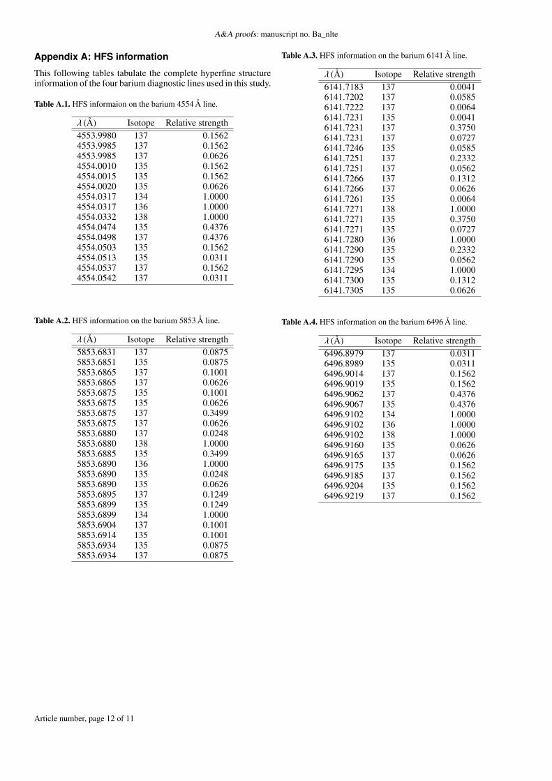
Appendix A: HFS information

This following tables tabulate the complete hyperfine structureinformation of the four barium diagnostic lines used in this study.

Table A.1. HFS informaion on the barium 4554 Å line.

λ (Å) Isotope Relative strength4553.9980 137 0.15624553.9985 137 0.15624553.9985 137 0.06264554.0010 135 0.15624554.0015 135 0.15624554.0020 135 0.06264554.0317 134 1.00004554.0317 136 1.00004554.0332 138 1.00004554.0474 135 0.43764554.0498 137 0.43764554.0503 135 0.15624554.0513 135 0.03114554.0537 137 0.15624554.0542 137 0.0311

Table A.2. HFS information on the barium 5853 Å line.

λ (Å) Isotope Relative strength5853.6831 137 0.08755853.6851 135 0.08755853.6865 137 0.10015853.6865 137 0.06265853.6875 135 0.10015853.6875 135 0.06265853.6875 137 0.34995853.6875 137 0.06265853.6880 137 0.02485853.6880 138 1.00005853.6885 135 0.34995853.6890 136 1.00005853.6890 135 0.02485853.6890 135 0.06265853.6895 137 0.12495853.6899 135 0.12495853.6899 134 1.00005853.6904 137 0.10015853.6914 135 0.10015853.6934 135 0.08755853.6934 137 0.0875


λ (Å) Isotope Relative strength6141.7183 137 0.00416141.7202 137 0.05856141.7222 137 0.00646141.7231 135 0.00416141.7231 137 0.37506141.7231 137 0.07276141.7246 135 0.05856141.7251 137 0.23326141.7251 137 0.05626141.7266 137 0.13126141.7266 137 0.06266141.7261 135 0.00646141.7271 138 1.00006141.7271 135 0.37506141.7271 135 0.07276141.7280 136 1.00006141.7290 135 0.23326141.7290 135 0.05626141.7295 134 1.00006141.7300 135 0.13126141.7305 135 0.0626


λ (Å) Isotope Relative strength6496.8979 137 0.03116496.8989 135 0.03116496.9014 137 0.15626496.9019 135 0.15626496.9062 137 0.43766496.9067 135 0.43766496.9102 134 1.00006496.9102 136 1.00006496.9102 138 1.00006496.9160 135 0.06266496.9165 137 0.06266496.9175 135 0.15626496.9185 137 0.15626496.9204 135 0.15626496.9219 137 0.1562


observational constraints on the origin of the elements

Documents