observations of the high redshift universe - arxiv · observations of the high redshift universe 5...
TRANSCRIPT

arX
iv:a
stro
-ph/
0701
024v
1 1
Jan
200
7
Observations of the High Redshift Universe
Richard S Ellis1
Astronomy Department, California Institute of [email protected]
ABSTRACT
In this series of lectures, aimed for non-specialists, I review the consider-able progress that has been made in the past decade in understanding howgalaxies form and evolve. Complementing the presentations of my theoreticalcolleagues, I focus primarily on the impressive achievements of observationalastronomers. A credible framework, the ΛCDM model, now exists for inter-preting these observations: this is a universe with dominant dark energy whosestructure grows slowly from the gravitational clumping of dark matter halosin which baryonic gas cools and forms stars. The standard model fares wellin matching the detailed properties of local galaxies, and is addressing thegrowing body of detailed multi-wavelength data at high redshift. Both thestar formation history and the assembly of stellar mass can now be empir-ically traced from redshifts z ≃6 to the present day, but how the variousdistant populations relate to one another and precisely how stellar assemblyis regulated by feedback and environmental processes remains unclear. In thelatter part of my lectures, I discuss how these studies are being extended to lo-cate and characterize the earliest sources beyond z ≃6. Did early star-forminggalaxies contribute significantly to the reionization process and over what pe-riod did this occur? Neither theory nor observations are well-developed in thisfrontier topic but the first results are exciting and provide important guidanceon how we might use more powerful future facilities to fill in the details.

2 Richard S Ellis
1 Role of Observations in Cosmology & Galaxy
Formation
1.1 The Observational Renaissance
These are exciting times in the field of cosmology and galaxy formation! Tojustify this claim it is useful to review the dramatic progress made in thesubject over the past ≃25 years. I remember vividly the first distant galaxyconference I attended: the IAU Symposium 92 Objects of High Redshift, held inLos Angeles in 1979. Although the motivation was strong and many observerswere pushing their 4 meter telescopes to new limits, most imaging detectorswere still photographic plates with efficiencies of a few percent and there wasno significant population of sources beyond a redshift of z=0.5, other thansome radio galaxies to z ≃1 and more distant quasars.
In fact, the present landscape in the subject would have been barely rec-ognizable even in 1990. In the cosmological arena, convincing angular fluc-tuations had not yet been detected in the cosmic microwave background norwas there any consensus on the total energy density ΩTOT . Although therole of dark matter in galaxy formation was fairly well appreciated, neitherits amount nor its power spectrum were particularly well-constrained. Thepresence of dark energy had not been uncovered and controversy still reignedover one of the most basic parameters of the Universe: the current expansionrate as measured by Hubble’s constant. In galaxy formation, although evolu-tion was frequently claimed in the counts and colors of galaxies, the physicalinterpretation was confused. In particular, there was little synergy betweenobservations of faint galaxies and models of structure formation.
In the present series of lectures, aimed for non-specialists, I hope to showthat we stand at a truly remarkable time in the history of our subject, largely(but clearly not exclusively) by virtue of a growth in observational capabili-ties. By the standards of all but the most accurate laboratory physicist, wehave ‘precise’ measures of the form and energy content of our Universe and adetailed physical understanding of how structures grow and evolve. We havesuccessfully charted and studied the distribution and properties of hundredsof thousands of nearby galaxies in controlled surveys and probed their lumi-nous precursors out to redshift z ≃6 - corresponding to a period only 1 Gyrafter the Big Bang. Most importantly, a standard model has emerged which,through detailed numerical simulations, is capable of detailed predictions andinterpretation of observables. Many puzzles remain, as we will see, but theprogress is truly impressive.
This gives us confidence to begin addressing the final frontier in galaxyevolution: the earliest stellar systems and their influence on the intergalacticmedium. When did the first substantial stellar systems begin to shine? Werethey responsible for reionizing hydrogen in intergalactic space and what phys-ical processes occurring during these early times influenced the subsequentevolution of normal galaxies?

Observations of the High Redshift Universe 3
Let’s begin by considering a crude measure of our recent progress. Figure1 shows the rapid pace of discovery in terms of the relative fraction of therefereed astronomical literature in two North American journals pertainingto studies of galaxy evolution and cosmology. These are cast alongside somemilestones in the history of optical facilities and the provision of widely-useddatasets. The figure raises the interesting question of whether more publica-tions in a given field means most of the key questions are being answered.Certainly, we can conclude that more researchers are being drawn to work inthe area. But some might argue that new students should move into other,less well-developed, fields. Indeed, the progress in cosmology, in particular, isso rapid that some have raised the specter that the subject may soon reachingsome form of natural conclusion (c.f. Horgan 1998).
Fig. 1. Fraction of the refereed astronomical literature in two North American jour-nals related to galaxy evolution and the cosmological parameters. The survey impliesmore than a doubling in fractional share over the past 15 years. Some possibly-associated milestones in the provision of unique facilities and datasets are marked(courtesy: J. Brinchmann).
I believe, however, that the rapid growth in the share of publications islargely a reflection of new-found observational capabilities. We are witnessingan expansion of exploration which will most likely be followed with a more

4 Richard S Ellis
detailed physical phase where we will be concerned with understanding howgalaxies form and evolve.
1.2 Observations Lead to Surprises
It’s worth emphasizing that many of the key features which define our currentview of the Universe were either not anticipated by theory or initially rejectedas unreasonable. Here is my personal short list of surprising observations whichhave shaped our view of the cosmos:
1. The cosmic expansion discovered by Slipher and Hubble during the pe-riod 1917-1925 was not anticipated and took many years to be accepted.Despite the observational evidence and the prediction from General Rela-tivity for evolution in world models with gravity, Einstein maintained hispreference for a static Universe until the early 1930’s.
2. The hot Big Bang picture received widespread support only in 1965 uponthe discovery of the cosmic microwave background (Penzias & Wilson1965). Although many supported the hypothesis of a primeval atom, Hoyleand others considered an unchanging ‘Steady State’ universe to be a morenatural solutuion.
3. Dark matter was inferred from the motions of galaxies in clusters overseventy years ago (Zwicky 1933) but no satisfactory explanation of thispuzzling problem was ever presented. The ubiquity of dark matter ongalactic scales was realized much later (Rubin et al 1976). The dominantrole that dark matter plays in structure formation only followed the recentobservational evidence (Blumenthal et al 1984).1
4. The cosmic acceleration discovered independently by two distant super-novae teams (Riess et al 1998, Perlmutter et al 1999) was a completesurprise (including to the observers, who set out to measure the deceler-ation). Although the cosmological constant, Λ, had been invoked manytimes in the past, the presence of dark energy was completely unforeseen.
Given the observational opportunities continue to advance. it seems rea-sonable to suppose further surprises may follow!
1.3 Recent Observational Milestones
Next, it’s helpful to examine a few of the most significant observationalachievements in cosmology and structure formation over the past ≃15 years.Each provides the basis of knowledge from which we can move forward, elim-inating a range of uncertainty across a wide field of research.
1 For an amusing musical history of the role of dark mat-ter in cosmology suitable for students of any age check outhttp://www-astronomy.mps.ohio-state.edu∼dhw/Silliness/silliness.html

Observations of the High Redshift Universe 5
The Rate of Local Expansion: Hubble’s Constant
The Hubble Space Telescope (HST) was partly launched to resolve the puz-zling dispute between various observers as regards to the value of Hubble’sconstant H0, normally quoted in kms sec−1 Mpc−1, or as h, the value in unitsof 100 kms sec−1 Mpc−1. During the planning phases, a number of scientifickey projects were defined and proposals invited for their execution.
A very thorough account of the impasse reached by earlier ground-basedobservers in the 1970’s and early 1980’s can be found in Rowan-Robinson(1985) who reviewed the field and concluded a compromise of 67 ± 15 kmssec−1 Mpc−1, surprisingly close to the presently-accepted value. Figure 2nicely illustrates the confused situation.
Fig. 2. Various values of Hubble’s constant in units of kms sec−1 Mpc−1 plotted asa function of the date of publication. Labels refer to estimates by Sandage & Tam-mann, de Vaucouleurs, van den Bergh and their respective collaborators. Estimatesfrom the HST Key Project group (Freedman et al 2001) are labeled KP. From an ini-tial range spanning 50< H0 <100, a gradual convergence to the presently-acceptedvalue is apparent. (Plot compiled and kindly made available by J. Huchra)
Figure 3 shows the two stage ‘step-ladder’ technique used by Freedman etal (2001) who claim a final value of 67 ± 15 kms sec−1 Mpc−1. ‘Primary’ dis-tances were estimated to a set of nearby galaxies via the measured brightnessand periods of luminous Cepheid variable stars located using HST’s WFPC-2

6 Richard S Ellis
imager. Over the distance range across which such individual stars can beseen (<25 Mpc), the leverage on H0 is limited and seriously affected by thepeculiar motions of the individual galaxies. At ≃20 Mpc, the smooth cosmicexpansion would give Vexp ≃1400 kms sec−1 and a 10% error in H0 wouldprovide a comparable contribution, at this distance, to the typical peculiarmotions of galaxies of Vpec ≃50-100 kms sec−1. Accordingly, a secondary dis-tance scale was established for spirals to 400 Mpc distance using the empiricalrelationship first demonstrated by Tully & Fisher (1977) between the I-bandluminosity and rotational velocity. At 400 Mpc, the effect of Vpec is negligibleand the leverage on H0 is excellent. Independent distance estimators utiliz-ing supernovae and elliptical galaxies were used to verify possible systematicerrors.
Fig. 3. Two step approach to measuring Hubble’s constant H0 - the local expansionrate (Freedman et al 2001). (Left) Distances to nearby galaxies within 25 Mpcwere obtained by locating and monitoring Cepheid variables using HST’s WFPC-2camera; the leverage on H0 is modest over such small distances and affected seriouslyby peculiar motions. (Right) Extension of the distance-velocity relation to 400 Mpcusing the I-band Tully-Fisher relation and other techniques. The absolute scale hasbeen calibrated using the local Cepheid scale.
Cosmic Microwave Background: Thermal Origin and Spatial
Flatness
The second significant milestone of the last 15 years is the improved under-standing of the cosmic microwave background (CMB) radiation, commencingwith the precise black body nature of its spectrum (Mather et al 1990) in-dicative of its thermal origin as a remnant of the cosmic fireball, and the sub-sequent detection of fluctuations (Smoot et al 1992), both realized with theCOBE satellite data. The improved angular resolution of later ground-basedand balloon-borne experiments led to the isolation of the acoustic horizon

Observations of the High Redshift Universe 7
scale at the epoch of recombination (de Bernadis et al 2000, Hanany et al2000). Subsequent improved measures of the angular power spectrum by theWilkinson Microwave Anisotropy Probe (WMAP, Spergel et al 2003, 2006)have refined these early observations. The location of the primary peak in theangular power spectrum at a multiple moment l ≃200 (corresponding to aphysical angular scale of ≃1 degree) provides an important constraint on thetotal energy density ΩTOT and hence spatial curvature.
The derivation of spatial curvature from the angular location of the firstacoustic (or ‘Doppler’) peak, θH , is not completely independent of other cos-mological parameters. There are dependences on the scale factor via H0 andthe contribution of gravitating matter ΩM , viz:
θH ∝ (ΩM h3.4)0.14Ω1.4TOT
where h is H0 in units of 100 kms sec−1 Mpc−1.However, in the latest WMAP analysis, combining with distant supernovae
data, space is flat to within 1%.
Clustering of Galaxies: Gravitational Instability
Galaxies represent the most direct tracer of the rich tapestry of structure inthe local Universe. The 1970’s saw a concerted effort to introduce a formalismfor describing and interpreting their statistical distribution through angularand spatial two point correlation functions (Peebles 1980). This, in turn, ledto an observational revolution in cataloging their distribution, first in 2-Dfrom panoramic photographic surveys aided by precise measuring machines,and later in 3-D from multi–object spectroscopic redshift surveys.
The angular correlation function w(θ) represents the excess probability δ Pof finding a pair of galaxies separated by an angular separation θ (degrees).
In a catalog averaging N galaxies per square degree, the probability offinding a pair separated by θ can be written:
δ P = N [1 + w(θ)]δ Ω
where δ Ω is the solid angle of the counting bin, (i.e. θ to θ + δ θ).The corresponding spatial equivalent, ξ(r) in a catalog of mean density ρ
per Mpc3 is thus:
δ P = ρ[1 + ξ(r)]δ V
One can be statistically linked to the other if the overall redshift distribu-tion of the sources is available.
Figure 4 shows a pioneering detection of the angular correlation functionw(θ) for the Cambridge APM Galaxy Catalog (Maddox et al 1990). This wasone of the first well-constructed panoramic 2-D catalogs from which the largescale nature of the galaxy distribution could be discerned. A power law formis evident:

8 Richard S Ellis
w(θ) = Aθ−0.8
where, for example, θ is measured in degrees. The amplitude A decreaseswith increasing depth due to both increased projection from physically-uncorrelated pairs and the smaller projected physical scale for a given angle.
Fig. 4. Angular correlation function for the APM galaxy catalog - a photographicsurvey of the southern sky (Maddox et al 1990) - partitioned according to limitingmagnitude (left). The amplitude of the clustering decreases with increasing depthdue to an increase in the number of uncorrelated pairs and a smaller projectedphysical scale for a given angle. These effects can be corrected in order to producea high signal/noise function scaled to a fixed depth clearly illustrating a universalpower law form over nearly 3 dex (right).
Highly-multiplexed spectrographs such as the 2 degree field instrument onthe Anglo-Australian Telescope (Colless et al 2001) and the Sloan Digital SkySurvey (York et al 2001) have led to the equivalent progress in 3-D surveys(Figure 5). In the early precursors to these grand surveys, the 3-D equivalentof the angular correlation function, was also found to be a power law:
ξ(r) = (r
r0)−1.8
where ro (Mpc) is a valuable clustering scale length for the population.As the surveys became more substantial, the power spectrum P (k) has
become the preferred analysis tool because its form can be readily predictedfor various dark matter models. For a given density field ρ(x), the fluctuation

Observations of the High Redshift Universe 9
over the mean is δ = ρ / ρ and for a given wavenumber k, the power spectrumbecomes:
P (k) =< |δ2k| >=
∫
ξ(r)exp(ik.r)d3r
The final power spectrum for the completed 2dF survey is shown in Figure6 (Cole et al 2005) and is in remarkably good agreement with that predictedfor a cold dark matter spectrum consistent with that which reproduces theCMB angular fluctuations.
Fig. 5. Galaxy distribution from the completed 2dF redshift survey (Colless et al2001).
Dark Matter and Gravitational Instability
We have already mentioned the ubiquity of dark matter on both cluster andgalactic scales. The former was recognized as early as the 1930’s from the highline of sight velocity dispersion σlos of galaxies in the Coma cluster (Zwicky1933). Assuming simple virial equilibrium and isotropically-arranged galaxyorbits, the cluster mass contained with some physical scale Rcl is:
M = 3 < σ2los > Rcl/G
which far exceeds that estimated from the stellar populations in the clustergalaxies. High cluster masses can also be confirmed completely independentlyfrom gravitational lensing where a background source is distorted to produce

10 Richard S Ellis
Fig. 6. Power spectrum from the completed 2dF redshift survey (Cole et al 2005).Solid lines refer to the input power spectrum for a dark matter model with the tab-ulated parameters and that convolved with the geometric ‘window function’ whichaffects the observed shape on large scales.
a ‘giant arc’ - in effect a partial or incomplete ‘Einstein ring’ whose diameterθE for a concentrated mass M approximates:
θE =4GM
1
2
c2D
1
2
and D = DsDl, /Dds where the subscripts s and l refer to angular diam-eters distances of the background source and lens respectively.
On galactic scales, extended rotation curves of gaseous emission lines inspirals (see review by Rubin 2000) can trace the mass distribution on theassumption of circular orbits, viz:
GM(< R)
R2=V 2
R
Flat rotation curves (V ∼constant) thus imply M(< R) ∝ R. Togetherwith arguments based on the question on the stability of flattened disks (Os-triker & Peebles 1973), such observations were critical to the notion that allspiral galaxies are embedded in dark extensive ‘halos’.
The evidence for halos around local elliptical galaxies is less convincinglargely because there are no suitable tracers of the gravitational potential onthe necessary scales (see Gerhard et al 2001). However, by combining grav-itational lensing with stellar dynamics for intermediate redshift ellipticals,Koopmans & Treu (2003) and Treu et al (2006) have mapped the projected

Observations of the High Redshift Universe 11
dark matter distribution and show it to be closely fit by an isothermal profileρ(r) ∝ r−2.
The presence of dark matter can also be deduced statistically from the dis-tortion of the galaxy distribution viewed in redshift space, for example in the2dF survey (Peacock et al 2001). The original idea was discussed by Kaiser etal (1987). The spatial correlation function ξ(r) is split into its two orthogonalcomponents, ξ(σ, π) where σ represents the projected separation perpendicu-lar to the line of sight (unaffected by peculiar motions) and π is the separationalong the line of sight (inferred from the velocities and hence used to mea-sure the effect). The distortion of ξ(σ, π) in the π direction can be measuredon various scales and used to estimate the line of sight velocity dispersionof pairs of galaxies and hence their mutual gravitational field. Depending onthe extent to which galaxies are biased tracers of the density field, such testsindicate ΩM=0.25.
On the largest scales, weak gravitational lensing can trace the overall distri-bution and dark matter content of the Universe (Blandford & Narayan 1992,Refregier 2003). Recent surveys are consistent with these estimates (Hoekstraet al 2005).
Dark Energy and Cosmic Acceleration
Prior to the 1980’s observational cosmologists were obsessed with two empiri-cal quantities though to govern the cosmic expansion history – R(t): Hubble’sconstant H0 = dR/dt and a second derivative, the deceleration parameter q0,which would indicate the fate of the expansion:
q0 = −d2R/dt2
(dR/dt)2
In the presence only of gravitating matter, Friedmann cosmologies indicateΩM = 2 q0. The distant supernovae searches were begun in the expectation ofmeasuring q0 independently of ΩM and verifying a low density Universe.
As we have discussed, Type Ia supernovae (SNe) were found to be fainter
at a given recessional velocity than expected in a Universe with a low massdensity; Figure 7 illustrates the effect for the latest results from the Canada-France SN Legacy Survey (Astier et al 2006). In fact the results cannot beexplained even in a Universe with no gravitating matter! A formal fit for q0indicates a negative value corresponding to a cosmic acceleration.
Acceleration is permitted in Friedmann models with a non-zero cosmolog-ical constant Λ. In general (Caroll et al 1992):
q0 =ΩM
2− 3
ΩΛ
2
where ΩΛ = Λ/8πG is the energy density associated with the cosmologicalconstant.

12 Richard S Ellis
Fig. 7. Hubble diagram (distance-redshift relation) for calibrated Type Ia super-novae from the first year data taken by the Canada France Supernova Legacy Survey(Astier et al 2006). Curves indicate the relation expected for a high density Universewithout a cosmological constant and that for the concordance cosmology (see text)
Observations of the High Redshift Universe 13
The appeal of resurrecting the cosmological constant is not only its abilityto explain the supernova data but also the spatial flatness in the acoustic peakin the CMB through the combined energy densities ΩM + ΩΛ - the so-calledConcordance Model (Ostriker & Steinhardt 1995, Bahcall et al 1999).
However, the observed acceleration raises many puzzles. The absolute valueof the cosmological constant cannot be understood in terms of physical de-scriptions of the vacuum energy density, and the fact that ΩM ≃ ΩΛ impliesthe accelerating phase began relatively recently (at a redshift of z≃0.7). Al-ternative physical descriptions of the phenomenon (termed ‘dark energy’) arethus being sought which can be generalized by imagining the vacuum obeys anequation of state where the negative pressure p relates to the energy densityρ via an index w,
p = w ρ
in which case the dependence on the scale factor R goes as
ρ ∝ R−3(1+w)
The case w=-1 would thus correspond to a constant term equivalent tothe cosmological constant, but in principle any w <-1/3 would produce anacceleration and conceivably w is itself a function of time. The current SNLSdata indicate w=-1.023 ± 0.09 and combining with the WMAP data does notsignificantly improve this constraint.
1.4 Concordance Cosmology: Why is such a curious model
acceptable?
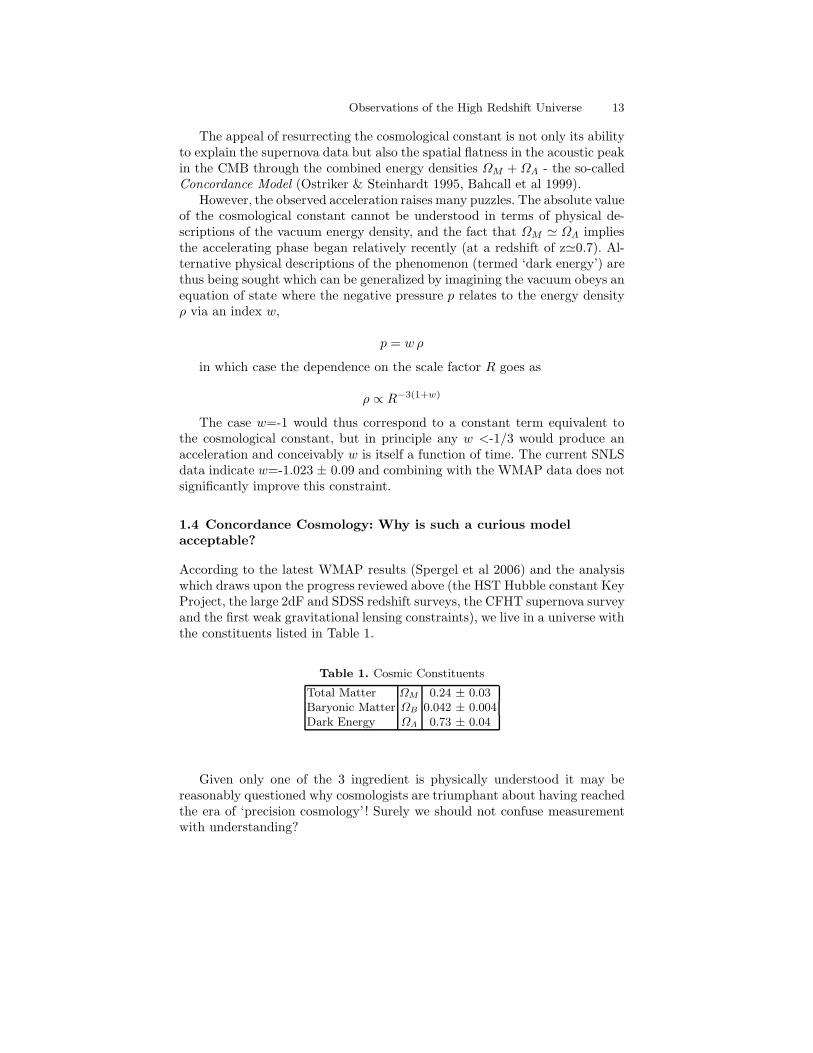
According to the latest WMAP results (Spergel et al 2006) and the analysiswhich draws upon the progress reviewed above (the HST Hubble constant KeyProject, the large 2dF and SDSS redshift surveys, the CFHT supernova surveyand the first weak gravitational lensing constraints), we live in a universe withthe constituents listed in Table 1.
Table 1. Cosmic Constituents
Total Matter ΩM 0.24 ± 0.03Baryonic Matter ΩB 0.042 ± 0.004Dark Energy ΩΛ 0.73 ± 0.04
Given only one of the 3 ingredient is physically understood it may bereasonably questioned why cosmologists are triumphant about having reachedthe era of ‘precision cosmology’ ! Surely we should not confuse measurementwith understanding?

14 Richard S Ellis
The underlying reasons are two-fold. Firstly, many independent probes(redshift surveys, CMB fluctuations and lensing) indicate the low matter den-sity. Two independent probes not discussed (primordial nucleosynthesis andCMB fluctuations) support the baryon fraction. Finally, given spatial flatness,even if the supernovae data were discarded, we would deduce the non-zero darkenergy from the above results alone.
Secondly, the above parameters reconcile the growth of structure from theCMB to the local redshift surveys in exquisite detail. Numerical simulationsbased on 1010 particles (e.g. Springel et al 2005) have reached the stage wherethey can predict the non-linear growth of the dark matter distribution atvarious epochs over a dynamic range of 3-4 dex in physical scales. Althoughsome input physics is needed to predict the local galaxy distribution, theagreement for the concordance model (often termed ΛCDM) is impressive. Inshort, a low mass density and non-zero Λ both seem necessary to explain thepresent abundance and mass distribution of galaxies. Any deviation wouldeither lead to too much or too little structure.
This does not mean that the scorecard for ΛCDM should be consideredperfect at this stage. As discussed, we have little idea what the dark matter ordark energy might be. Moreover, there are numerous difficulties in reconcil-ing the distribution of dark matter with observations on galactic and clusterscales and frequent challenges that the mass assembly history of galaxies isinconsistent with the slow hierarchical growth expected in a Λ-dominated Uni-verse. However, as we will see in later lectures, most of these problems relateto applications in environments where dark matter co-exists with baryons.Understanding how to incorporate baryons into the very detailed simulationsnow possible is an active area where interplay with observations is essential.It is helpful to view this interplay as a partnership between theory and obser-vation rather than the oft-quoted ‘battle’ whereby observers challenge or callinto question the basic principles.
1.5 Lecture Summary
I have spent my first lecture discussing largely cosmological progress and theimpressive role that observations have played in delivering rapid progress.
All the useful cosmological functions - e.g. time, distance and comovingvolume versus redshift, are now known to high accuracy which is tremendouslybeneficial for our task in understanding the first galaxies and stars. I emphasizethis because even a decade ago, none of the physical constants were knownwell enough for us to be sure, for example, the cosmic age corresponding to aparticular redshift.
I have justified ΛCDM as an acceptable standard model, despite the un-known nature of its two dominant constituents, partly because there is a con-cordance in the parameters when viewed from various observational probes,and partly because of the impressive agreement with the distribution of galax-ies on various scales in the present Universe.
Observations of the High Redshift Universe 15
Connecting the dark matter distribution to the observed properties ofgalaxies requires additional physics relating to how baryons cool and formstars in dark matter halos. Detailed observations are necessary to ‘tune’ themodels so these additional components can be understood.
All of this will be crucial if we are correctly predict and interpret signalsfrom the first objects.

16 Richard S Ellis
2 Galaxies & the Hubble Sequence
2.1 Introduction: Changing Paradigms of Galaxy Formation
We now turn to the interesting history of how our views of galaxy formationhave changed over the past 20-30 years. It is convenient to break this into 3eras
1. The classical era (pre-1985) as articulated for example in the influentialarticles by Beatrice Tinsley and others. Galaxies were thought to evolve inisolation with their present-day properties governed largely by one func-tion - the time-dependent star formation rate ψ(t). Ellipticals suffered aprompt conversion of gas into stars, whereas spirals were permitted a moregradual consumption rate leading to a near-constant star formation ratewith time.
2. The dark matter-based era (1985-): in hierarchical models of structureformation involving gravitational instability, the ubiquity of dark matterhalos means that merger driven assembly is a key feature. If mergersredistribute angular momentum, galaxy morphologies are transformed.
3. Understanding feedback and the environment (1995-): In the most re-cent work, the evolution of the morphology-density relation (Dressler etal 1997) and the dependence of the assembly history on galactic mass(‘downsizing’, Cowie et al 1996) have emphasized that star formation isregulated by processes other than gas cooling and infall associated withDM-driven mergers.
2.2 Galaxy Morphology - Valuable Tool or Not?
In the early years, astronomers placed great stock on understanding the ori-gin of the morphological distribution of galaxies, sometimes referred to as theHubble sequence (Hubble 1936). Despite this simple categorization 70 yearsago, the scheme is evidently still in common use. In its support, Sandage (e.g.2005) has commented on this classification scheme as describing ‘a true orderamong the galaxies, not one imposed by the classifier’. However, many con-temporary modelers and observers have paid scant attention to morphologyand placed more emphasis on understanding stellar population differences.What value should we place on accurately measuring and reproducing themorphological distribution?
The utility of Hubble’s scheme, at least for local galaxies, lies in its abilityto distinguish dynamically distinct structures - spirals and S0s are rotatingstellar disks, whereas luminous spheroids are pressure-supported ellipsoidal ortriaxial systems with anisotropic velocity fields. This contains key informationon the degree of dissipation in their formation (Fall & Efstathiou 1980).
There are also physical variables that seem to underpin the sequence,including (i) gas content and color which relate to the ratio of the current to

Observations of the High Redshift Universe 17
past average star formation ratio ψ(t0)/ ψ (Figure 8) and (ii) inner structuresincluding the bulge-to-disk ratio. Various modelers (Baugh et al 1996) haveargued that the bulge-to-disk ratio is closely linked to the merger history andattempted to reproduce the present distribution as a key test of hierarchicalassembly.
Fig. 8. A succinct summary of the classical view of galaxy formation (pre-1985):(Left) The monotonic distribution of Hubble sequence galaxies in the U−V vs V −Kcolor plane (Aaaronson 1978). (Right) A simple model which reproduces this trendby changing only the ratio of the current to past average star formation rate (Struck-Marcell & Tinsley 1978). Galaxies with constant star formation permanently occupythe top left (blue) corner; galaxies with an initial burst rapidly evolve to the bottomright (red) corner.
Much effort has been invested in attempting to classify galaxies at highredshift, both visually and with automated algorithms. This is a challengingtask because the precise appearance of diagnostic features such as spiral armsand the bulge/disk ratio depends on the rest-wavelength of the observations.An effect termed the ‘morphological k-correction’ can thus shift galaxies toapparently later types as the redshift increases for observations conductedin a fixed band. A further limitation, which works in the opposite sense, issurface brightness dimming, which proceeds as ∝ (1 + z)4, rendering disksless prominent at high redshift and shifting some galaxies to apparent earlier
types.The most significant achievements from this effort has been the realization
that, despite the above quantitative uncertainties, faint star-forming galaxiesare generally more irregular in their appearance than in local samples (Glaze-brook et al 1995, Driver et al 1995). Moreover, HST images suggest on-goingmergers with an increasing frequency at high redshift (LeFevre et al 2000) al-

18 Richard S Ellis
though quantitative estimates of the merging fraction as a function of redshiftremain uncertain (see Bundy et al 2004).
The idea that morphology is driven by mergers took some time for the ob-servational community to accept. Numerical simulations by Toomre & Toomre(1972) provided the initial theoretical inspiration, but the observational ev-idence supporting the notion that spheroidal galaxies were simple collapsedsystems containing old stars was strong (Bower et al 1992). Tell-tale signsof mergers in local ellipticals include the discovery of orbital shells (Malin& Carter 1980) and multiple cores revealed only with 2-D dynamical studies(Davies et al 2001).
2.3 Semi-Analytical Modeling
As discussed by the other course lecturers and briefly in §1, our ability to followthe distribution of dark matter and its growth in numerical simulations is well-advanced (e.g. Springel et al 2005). The same cannot be said of understandinghow the baryons destined, in part, to become stars are allocated to each DMhalo. This remains the key issue in interfacing theory to observations.
Progress has occurred in two stages - according to the eras discussedin §2.1. Semi analytic codes were first developed in the 1990’s to introducebaryons into DM n-body simulations using prescriptive methods for star for-mation, feedback and morphological assembly (Figure 9). These codes wereinitially motivated to demonstrate that the emerging DM paradigm was con-sistent with the abundance of observational data (Kauffmann et al 1993,Somerville & Primack 1999, Cole et al 2000). Prior to development of thesecodes, evolutionary predictions were based almost entirely on the ‘classical’viewpoint with stellar population modeling based on variations in the starformation history ψ(t) for galaxies evolving in isolation e.g. Bruzual (1980).
Initially these feedback prescriptions were adjusted to match observablessuch as the luminosity function (whose specific details we will address below),as well as specific attributes of various surveys (counts, redshift distributions,colors and morphologies). In the recent versions, more elaborate physically-based models for feedback processes are being considered (e.g. Croton et al2006)
The observational community was fairly skeptical of the predictions fromthe first semi-analytical models since it was argued that the parameter spaceimplied by Figure 9 enabled considerable freedom even for a fixed primor-dial fluctuation spectrum and cosmological model. Moreover, where differentcodes could be compared, considerably different predictions emerged (Bensonet al 2002). Only as the observational data has moved from colors and starformation rates to physical variables more closely related to galaxy assem-bly (such as stellar masses) have the limitations of the early semi-analyticalmodels been exposed.

Observations of the High Redshift Universe 19
Fig. 9. Schematic of the ingredients inserted into a semi-analytical model (fromCole et al 2000). Solid lines refer to mass transfer, dashed lines to the transfer ofmetals according to different compositions Z. Gas cooling (M) and star formation(ψ) is inhibited by the effect of supernovae (β). Stars return some fraction of theirmass to the interstellar medium (R) and to the hot gas phase (e) according to ametal yield p.
2.4 A Test Case: The Galaxy Luminosity Function
One of the most straightforward and fundamental predictions a theory ofgalaxy formation can make is the present distribution of galaxy luminosities- the luminosity function (LF) Φ(L) whose units are normally per comovingMpc3 2.
As the contribution of a given luminosity bin dL to the integrated luminos-ity density per unit volume is ∝ Φ(L)LdL, an elementary calculation showsthat all luminosity functions (be they for stars, galaxies or QSOs) must have abend at some characteristic luminosity, otherwise they would yield an infinitetotal luminosity (see Felton 1977 for a cogent early discussion of the signifi-cance and intricacies of the LF). Recognizing this, Schechter (1976) proposedthe product of a power law and an exponential as an appropriate analyticrepresentation of the LF, viz:
Φ(L)dL
L∗= Φ∗(
L
L∗)−α exp(−
L
L∗)dL
L∗
where Φ∗ is the overall normalization corresponding to the volume densityat the turn-over (or characteristic) luminosity L∗, and α is the faint end slopewhich governs the relative abundance of faint and luminous galaxies.
The total abundance of galaxies per unit volume is then:
2 If Hubble’s constant is not assumed, it is quoted in units of h−3 Mpc−3

20 Richard S Ellis
NTOT =
∫
Φ(L) dL = Φ∗ Γ (α+ 1)
and the total luminosity density is:
ρL =
∫
Φ(L)LdL = Φ∗ Γ (α+ 2)
where Γ is the incomplete gamma function which can be found tabulatedin most books with integral tables (e.g. Gradshteyn & Ryzhik 2000). Notethat NTOT diverges if α <-1, whereas ρL diverges only if α <-2.
Recent comprehensive surveys by the 2dF team (Norberg et al 2002) andby the Sloan Digital Sky Survey (Blanton et al 2001) have provided definitivevalues for the LF in various bands. Encouragingly, when allowance is madefor the various photometric techniques, the two surveys are in excellent agree-ment. Figure 10 shows the Schechter function is a reasonably good (but notperfect) fit to the 2dF data limited at apparent magnitude bJ <19.7. Moreoverthere is no significant difference between the LF derived independently for thetwo Galactic hemispheres. The slight excess of intrinsically faint galaxies inthe northern cap is attributable to a local inhomogeneity in the nearby Virgosupercluster.
Fundamental though this function is, despite ten years of semi-analyticalmodeling, reproducing its form has proved a formidable challenge (as discussedby Benson et al 2003, Croton et al 2006 and de Lucia et al 2006). Earlypredictions also failed to reproduce the color distribution along the LF. Thehalo mass distribution does not share the sharp bend at L∗ and too much starformation activity is retained in massive galaxies. These early predictionsproduced too many luminous blue galaxies and too many faint red galaxies(Bower et al 2006).
As a result, more specific feedback recipes have been created to resolvethis discrepancy. Several physical processes have been invoked to regulatestar formation as a function of mass, viz:
• Reionization feedback: radiative heating from the first stellar systems athigh redshift which increases the Jeans mass, inhibiting the early formationof low mass systems,
• Supernova feedback: this was considered in the early semi-analytical mod-els but is now more precisely implemented so as to re-heat the interstellarmedium, heat the halo gas or even eject the gas altogether from low masssystems,
• Feedback from active galactic nuclei: the least well-understood processwith various modes postulated to transfer energy from an active nucleusto the halo gas.
Benson et al (2003) and Croton et al (2006) illustrate the effects of thesemore detailed prescriptions for these feedback modes on the predicted LF andfind that supernova and reionization feedback largely reduce the excess of

Observations of the High Redshift Universe 21
Fig. 10. Rest-frame bJ luminosity function from the 2dF galaxy redshift survey(Norberg et al 2002). (Top) a comparison of results across the northern and southernGalactic caps; there is only a marginal difference in the abundance of intrinsicallyfaint galaxies. (Bottom) combined from both hemispheres indicating the Schechterfunction is a remarkably good fit except at the extreme ends of the luminositydistribution.
intrinsically faint galaxies but, on grounds of energetics, only AGN can inhibitstar formation and continued growth in massive galaxies. There remains anexcess at the very faint end (Fig. 11).
2.5 The Role of the Environment
In addition to recognizing that more elaborate modes of feedback need to beincorporated in theoretical models, the key role of the environment has also

22 Richard S Ellis
Fig. 11. The effect of various forms of feedback (dots) on the resultant shape of theblue 2dF galaxy luminosity function (Norberg et al 2002). From left to right: no feed-back, supernova feedback only, supernova, reionization & AGN feedback (Courtesy:Darren Croton).
emerged as an additional feature which can truncate star formation and altergalaxy morphologies.
The preponderance of elliptical and S0 galaxies in rich clusters was no-ticed in the 1930’s but the first quantitative study of this effect was that ofDressler (1980) who correlated the fraction of galaxies of a given morphologyT above some fixed luminosity with the projected galaxy density, Σ, measuredin galaxies Mpc−2.
The local T − Σ relation was used to justify two rather different possi-bilities. In the first, the nature hypothesis, those galaxies which formed inhigh density peaks at early times were presumed to have consumed their gasefficiently, perhaps in a single burst of star formation. Galaxies in lower den-sity environments continued to accrete gas and thus show later star formationand disk-like morphologies. In short, segregation was established at birth andthe present relation simply represents different ways in which galaxies formedaccording to the density of the environment at the time of formation. In thesecond, the nurture hypothesis, galaxies are transformed at later times fromspirals into spheroidals by environmentally-induced processes.
Work in the late 1990’s, using morphologies determined using HubbleSpace Telescope, confirmed a surprisingly rapid evolution in the T−Σ relationover 0< z <0.5 (Couch et al 1998, Dressler et al 1997) strongly supportingenvironmentally-driven evolution along the lines of the nurture hypothesis.Impressive Hubble images of dense clusters at quite modest redshifts (z ≃0.3-0.4) showed an abundance of spirals in their cores whereas few or none existin similar environs today.
What physical processes drive this relation and how has the T −Σ relationevolved in quantitative detail? Recent work (Smith et al 2005, Postman et al2005, Figure 12) has revealed that the basic relation was in place at z ≃1,but that the fraction fE+S0 of Es and S0s has doubled in dense environmentssince that time. Smith et al suggest that a continuous, density-dependent,

Observations of the High Redshift Universe 23
transformation of spirals into S0s would explain the overall trend. Treu et al(2003) likewise see a strong dependence of the fraction as a function of Σ (andto a lesser extent with cluster-centric radius) within a well-studied cluster atz ≃0.4; they review the various physical mechanisms that may produce sucha transformation.
Fig. 12. The fraction of observed E and S0 galaxies down to a fixed rest-frameluminosity as a function of lookback time and projected density Σ from the study ofSmith et al (2005). Although the morphology density relation was already in placeat z ≃1, there has been a continuous growth in the fraction subsequently, possiblyas a result of the density-dependent transformation of spirals into S0s.
Figure 12 encapsulates much of what we now know about the role of theenvironment on galaxy formation. The early development of the T − Σ re-lation implies dense peaks in the dark matter distribution led to acceleratedevolution in gas consumption and stellar evolution and this is not dissimilar tothe nature hypothesis. However, the subsequent development of this relationsince z ≃1 reveals the importance of environmentally-driven morphologicaltransformations.
2.6 The Importance of High Redshift Data
This glimpse of evolving galaxy populations to z ≃1 has emphasized theimportant role of high redshift data. In the case of the local morphology-density relation, Hubble morphologies of galaxies in distant clusters have givenus a clear view of an evolving relationship, partly driven by environmental

24 Richard S Ellis
processes. Indeed, the data seems to confirm the nurture hypothesis for theorigin of the morphology-density relation.
Although we can place important constraints on the past star formationhistory from detailed studies of nearby galaxies, as the standard model nowneeds several additional ingredients (e.g. feedback) to reproduce even the mostbasic local properties such as the luminosity function (Figure 11), data atsignificant look-back times becomes an essential way to test the validity ofthese more elaborate models.
Starting in the mid-1990’s, largely by virtue of the arrival of the Kecktelescopes - the first of the new generation of 8-10m class optical/infraredtelescopes - and the refurbishment of the Hubble Space Telescope, there hasbeen an explosion of new data on high redshift galaxies.
It is helpful at this stage to introduce three broad classes of distant ob-jects which will feature significantly in the next few lectures. Each gives acomplementary view of the galaxy population at high redshift and illustratesthe challenge of developing a unified vision of galaxy evolution.
Fig. 13. Location and verification of the Lyman break population in the redshiftrange 2.7< z <3.4 (Steidel et al 2003). (Left) UGR color-color plane for a single field;green and yellow shading refers to variants on the color selection of high redshiftcandidates. Contaminating Galactic stars cut across the lower right corner of thisselection; those confirmed spectroscopically are marked in red. (Right) Coaddedrest-frame Keck spectra for samples of typically 200 Lyman break galaxies binnedaccording to the strength of Lyman α emission.

Observations of the High Redshift Universe 25
• Lyman-break galaxies: color-selected luminous star forming galaxies at
z >2. First located spectroscopically by Steidel et al (1996, 1999a, 1999b,2003), these sources are selected by virtue of the increased opacity short-ward of the Lyman limit (λ =912A ) arising from the combined effectof neutral hydrogen in hot stellar atmospheres, the interstellar gas andthe intergalactic medium. When redshifted beyond z≃2, the characteristic‘drop out’ in the Lyman continuum moves into the optical (Figure 13). Wewill review the detailed properties of this, the most well-studied, distantgalaxy population over 2< z <5 in subsequent lectures.
Fig. 14. Redshift distribution of 73 radio-identified SCUBA sources from Chapmanet al (2005). To illustrate the possible bias arising from the necessary condition ofa radio position for a Keck redshift, the solid curve represents a model predictionfor the entire >5mJy sub-mm population. The sub-mm population does not seemto extend significantly beyond z≃4 and has a median redshift of z=2.2.
• Sub-millimeter star forming sources: The SCUBA 850µm array on the 15meter James Clerk Maxwell Telescope and other sub-mm imaging deviceshave also been used to locate distant star forming galaxies (Smail et al1997, Hughes et al 1998). In this case, emission is detected from dust,heated either by vigorous star formation or an active nucleus. Remarkably,their visibility does not fall off significantly with redshift because they aredetected in the Rayleigh-Jeans tail of the dust blackbody spectrum (Blainet al 2002).

26 Richard S Ellis
Progress in understanding the role and nature of this population has beenslower because sub-mm sources are often not visible at optical and near-infrared wavelengths (due to obscuration) and the positional accuracy ofthe sub-mm arrays is too coarse for follow-up spectroscopy. The impor-tance of sub-mm sources lies in the fact that they contribute significantlyto the star formation rate at high redshift. Regardless of their redshift, thesource density at faint limits is 1000 times higher than a no-evolution pre-diction based on the local abundance of dusty IRAS sources. For severalyears the key issue was to nail the redshift distribution.Progress has been made by securing accurate positions using radio interfer-ometers such as the VLA (Frayer et al 2000). About 70% of those brighterthan 5 mJy have VLA detections and spectroscopic redshift have nowbeen determined for a significant fraction of this population (Chapman etal 2003, 2005, Figure 14).
Fig. 15. Observed spectral energy distribution of distant red sources selected witha red J−K color superimposed on model spectra (Franx et al 2003). Although somesources reveal modest star formation and can be spectroscopically confirmed to lieabove z ≃2, others (such as the lower two examples) appear to be passively-evolvingwith no active star formation.
• Passively-Evolving Sources: The Lyman-break and sub-mm sources arelargely star-forming galaxies. The arrival of panoramic near-infrared cam-eras has opened the possibility of locating quiescent sources that are nolonger forming stars. Such sources would not normally be detected via the

Observations of the High Redshift Universe 27
other techniques and so understanding their contribution to the integratedstellar mass at, say, z ≃2, is very important.The nomenclature here is confusing with intrinsically red sources beingtermed ‘extremely red objects (EROs)’ or ‘distant red galaxies (DRGs)’with no agreed selection criteria (see McCarthy 2004 for a review). Whenstar formation is complete, stellar evolution continues in a passive sensewith main sequence dimming; the galaxy fades and becomes redder.Of particular interest are the most distant examples which co-exist along-side the sub-mm and Lyman-break galaxies, i.e. at z >2 selected accordingto their infrared J −K color (van Dokkum et al 2003, Figure 15).
2.7 Lecture Summary
We have seen in this brief tour that galaxy formation is a process involvinggravitational instability driven by the hierarchical assembly of dark matterhalos; this component we understand well. However, additional complexitiesarise from star formation, dynamical interactions and mergers, environmentalprocesses and various forms of feedback which serve to regulate how starformation continues as galaxies grow in mass.
Theorists have attempted to deal with this complexity by augmenting thehighly-successful numerical (DM-only) simulations with semi-analytic toolsfor incorporating these complexities. As the datasets have improved so it isnow possible to consider ‘fine-tuning’ these semi-analytical ingredients. Ab
initio modeling is never likely to be practical.I think it fair to say that many observers have philosophical reservations
about this ‘fine-tuning’ process in the sense that although it may be possibleto reach closure on models and data, we seek a deeper understanding of thephysical reality of many of the ingredients. This is particularly the case forfeedback processes. Fortunately, high redshift data forces this reality check asit gives us a direct measure of the galaxy assembly history which will be thenext topics we discuss.
As a way of illustrating the importance of high redshift data, I have in-troduced three very different populations of galaxies each largely lying inthe redshift range 2< z <4. When these were independently discovered, itwas (quite reasonably) claimed by their discoverers that their category repre-sented a major, if not the most significant, component of the distant galaxypopulation. We now realize that UV-selected, sub-mm selected and non-starforming galaxies each provide a complementary view of the complex historyof galaxy assembly and the challenge is to complete the ‘jig-saw’ from thesepopulations.

28 Richard S Ellis
3 Cosmic Star Formation Histories
3.1 When Did Galaxies Form? Searches for Primeval Galaxies
The question of the appearance of an early forming galaxy goes back to the1960’s. Partride & Peebles (1967) imagined the free-fall collapse of a 700 L∗
system at z ≃10 and predicted a diffuse large object with possible Lyman αemission. Meier (1976) considered primeval galaxies might be compact andintense emitters such as quasars.
In the late 1970’s and 1980’s when the (then) new generation of 4 metertelescopes arrived, astronomers sought to discover the distinct era when galax-ies formed. Stellar synthesis models (Tinsley 1980, Bruzual 1980) suggestedpresent-day passive systems (E/S0s) could have formed via a high redshift lu-minous initial burst. Placed at z ≃2-3, sources of the same stellar mass wouldbe readily detectable at quite modest magnitudes, B ≃22-23, and provide anexcess population of blue galaxies.
In reality, the (now well-studied) excess of faint blue galaxies over locally-based predictions is understood to be primarily a phenomenon associated witha gradual increase in star formation over 0 < z <1 rather than one due to adistinct new population of intensely luminous sources at high redshift (Koo& Kron 1992, Ellis 1997). Moreover, dedicated searches for suitably intenseLyman α emitters were largely unsuccessful. Pritchet (1994) comprehensivelyreviews a decade of searching.
Our thinking about primeval galaxies changed in two respects in the late1980’s. Foremost, synthesis models such as those developed by Tinsley andBruzual assumed isolated systems; dark matter-based models emphasized thegradual assembly of massive galaxies. This change meant that, at z ≃2-3,the abundance of massive galaxies should be much reduced. Secondly, theflux limits searched for primeval galaxies were optimistically bright; we slowlyrealized the more formidable challenge of finding these enigmatic sources.
3.2 Local Inventory of Stars
An important constraint on the past star formation history is the present-daystellar density. The former must, when integrated, yield the latter. Fukugitaet al (1998) and Fukugita & Peebles (2004) have considered this importantproblem based on local survey data provided by the SDSS (Kauffmann et al2003) and 2dF (Cole et al 2001) redshift samples.
The derivation of the integrated density of stars involves many assump-tions and steps but is based primarily on the local infrared (K-band) lumi-nosity function of galaxies. The rest-frame K luminosity of a galaxy is a muchmore reliable proxy for its stellar mass than that at a shorter (e.g. optical)wavelength because its value is largely irrespective of the past star formationhistory - a point illustrated by Kauffmann & Charlot (1998, Figure 16). An-other way to phrase this is to say that the infrared mass/light ratio (M/LK)

Observations of the High Redshift Universe 29
is fairly independent of the star formation history, so that the stellar mass canbe derived from the observed K-band luminosity by a multiplicative factor.
Fig. 16. The robustness of the K-band luminosity of a galaxy as a proxy for stellarmass (Kauffmann & Charlot 1998). The upper panel shows the K-band apparentmagnitude of a galaxy defined to have a fixed stellar mass of 1011M⊙ when placedat various redshifts. The different curves represent extreme variations in the waythe stellar population was created. Whereas the B −K color is strongly dependentupon the star formation history, the K-band luminosity is largely independent of it.
In practice the mass/light ratio depends on the assumed distribution ofstellar masses in a stellar population. The zero age or initial mass function isusually assumed to be some form of power law which can only be determinedreliable for Galactic stellar populations, although constraints are possible forextragalactic populations from colors and nebular line emission (see reviewsby Scalo 1986, Kennicutt 1998, Chabrier 2003)
In its most frequently-used form the IMF is quoted in mass fraction perlogarithmic mass bin: viz:
ξ(log m) =dn
d logm∝ m−x
or, occasionally,

30 Richard S Ellis
ξ(m) =dn
dm=
1
m(ln 10)ξ(logm) ∝ m−α
where x = α− 1.In his classic derivation of the IMF, Salpeter (1955) determined a pure
power law with x=1.35. More recently adopted IMFs are compared in Figure17. They differ primarily in how to restrict the low mass contribution, butthere is also some dispute on the high mass slope (although the Salpeter valueis supported by various observations of galaxy colors and Hα distributions,Kennicutt 1998).
Fig. 17. A comparison of popular stellar initial mass functions (courtesy of IvanBaldry).
The IMF has a direct influence on the assumed M/LK (as discussed byBaldry & Glazebrook 2003, Chabrier, 2003 and Fukugita & Peebles, 2004) ina manner which depends on the age, composition and past star formation his-tory. The adopted mass/light ratio is then a crucial ingredient for computingboth stellar masses (LectureLecture 4) and galaxy colors.
Baldry3 has undertaken a very useful comparative study of the impact ofvarious IMF assumptions using the PEGASE 2.0 stellar synthesis code fora population 10 Gyr old with solar metallicity, integrating between stellar
3 http://www.astro.livjm.ac.uk∼ikb/research/imf-use-in-cosmology.html

Observations of the High Redshift Universe 31
Table 2. K-band Stellar Mass/Light Ratios
Source Stars Stars + WDs/BHs Total (Past SFR)
Salpeter (1955) 1.15 1.30 1.86Miller Scalo (1979) 0.46 0.60 0.99Kennicutt (1983) 0.46 0.60 1.06Scalo (1986) 0.52 0.61 0.84Kroupa et al (1993) 0.65 0.76 1.09Kroupa (2001) 0.67 0.83 1.48Baldry & Glazebrook (2003) 0.67 0.86 1.76Chabrier (2003) 0.59 0.75 1.42
masses of 0.1 and 120 M⊙ (Table 2). Stellar masses have been defined invarious ways as represented by the 3 columns in Table 2. Typically we areinterested in the observable stellar mass at a given time (i.e. main sequenceand giant branch stars), but it is interesting to also compute the total masswhich is not in the interstellar medium, which includes that locked in evolveddegenerate objects (white dwarfs and black holes). The most inclusive defini-tion of stellar mass (total) is the integral of the past star formation history.Depending on the definition, and chosen IMF, the uncertainties range almostover a factor of 4 for the most popularly-used functions, quite apart from theunsettling question of whether the form of the IMF might vary with epoch ortype of object.
Although the stellar mass function for a galaxy survey can be derivedassuming a fixed mass/light ratio, the useful stellar density is that correctedfor the fractional loss, R, of stellar material due to winds and supernovae.Only with this correction (R=0.28 for a Salpeter IMF), does the present-dayvalue represent the integral of the past star formation.
Figure 18 shows the K-band luminosity and derived stellar mass functionfor galaxies in the 2dF redshift survey from the analysis of Cole et al (2001).K-band measures were obtained by correlation with the K <13.0 catalogobtained by the 2MASS survey.
The integrated stellar density, corrected for stellar mass loss, is (Cole etal 2001):
Ωstars h = 0.0027 ± 0.00027
for a Salpeter IMF, a value very similar to that derived independently byFukugita & Peebles (2004). By comparison the local mass fraction in neutralHI + He I gas is:
Ωgas h = 0.00078 ± 0.00016
Thus only 5% of all baryons are in stars with the bulk in ionized gas.

32 Richard S Ellis
Fig. 18. (Left) Rest-frame K-band luminosity function derived from the combi-nation of redshifts from the 2dF survey with photometry from 2MASS (Cole et al2001); Schechter parameter fits are shown. (Right) Derived stellar mass functionassuming a Salpeter IMF corrected for lost material assuming R=0.28 (see text).
3.3 Diagnostics of Star Formation in Galaxies
When significant redshift surveys became possible at intermediate and highredshift through the advent of multi-object spectrographs, so it became pos-sible to consider various probes of the star formation rate (SFR) at differentepochs. As in the formalism for calculating the integrated luminosity density,ρL, per comoving Mpc3, so for a given population various diagnostics of on-going star formation can yield an equivalent global star formation rate ρSFR
in units of M⊙ yr−1 Mpc−3.Such integrated measures average over a whole host of important de-
tails, such as differences in evolutionary behavior between luminous and sub-luminous galaxies and, of course, morphology. Moreover, in any survey athigh redshift, only a portion of the population is rendered visible so uncertaincorrections must be made to compare results at different epochs. The impor-tance of the cosmic star formation history, i.e. ρSFR(z), is it displays, in asimple manner, the epoch and duration of galaxy growth. By integrating thefunction, one should recover the present stellar density (§3.5).
There are various probes of star formation in galaxies, each with its ad-vantages and drawbacks. Not only is there no single ‘best’ method to gaugethe current star formation rate of a chosen galaxy, but as each probe samplesthe effect of young stars in different initial mass ranges, so each averages thestar formation rate over a different time interval. If, as is often the case in themost energetic sources, the star formation is erratic or burst-like, one wouldnot expect different diagnostics to give the same measure of the instantaneousSFR even for the same galaxies.

Observations of the High Redshift Universe 33
Four diagnostics are in common use (see review by Kennicutt 1998).
• The rest-frame ultraviolet continuum (λλ ≃1250-1500A ) has the advan-tage of being directly connected to well-understood high mass (> 5M⊙)main sequence stars. Large datasets are available for high redshift star-forming galaxies, including some to z ≃6. Via the GALEX satellite andearlier balloon-borne experiments, local data is also available. The disad-vantage of this diagnostic lies in the uncertain (and significant) correctionsnecessary for dust extinction and a modest sensitivity to the assumed ini-tial mass function. Obscured populations are completely missed in UVsamples. Kennicutt suggests the following calibration for the UV luminos-ity:
SFR(M⊙yr−1) = 1.4 10−28Lν(ergs s−1Hz−1)
• Nebular emission lines such as Hα and [O II] are also available for a rangeof redshifts (z < 2.5), for example as a natural by-product of faint redshiftsurveys. Gas clouds are photo-ionized by very massive (> 10M⊙) stars.Dust extinction can often be evaluated from higher order Balmer linesunder various radiative assumptions depending on the escape fraction ofionizing photons. The sensitivity to the initial mass function is strong.
SFR(M⊙yr−1) = 7.9 10−42L(Hα)(ergs s−1)
SFR(M⊙yr−1) = 1.4 ± 0.410−41L(OII)(ergs s−1)
• Far infrared emission (10-300 µm) arises from dust heated by young stars.It is clearly only a tracer in the most dusty systems and thus acts as avaluable complementary probe to the UV continuum. As we have seen in§2, luminous far infrared galaxies are also seen to high redshift. However,not all dust heating is due to young stars and the bolometric far infraredflux, LFIR, is needed for an accurate measurement.
SFR(M⊙yr−1) = 4.5 10−44LFIR(ergs s−1)
• Radio emission, e.g. at 1.4GHz, is thought to arise from synchrotron emis-sion generated by relativistic electrons accelerated by supernova remnantsfollowing the rapid evolution of the most massive stars. Its great advan-tage is that it offers a dust-free measure of the recent SFR. Current radiosurveys do not have the sensitivity to see emission beyond z ≃1, so itspromise has yet to be fully explored. This process is also the least well-understood and calibrated. Sullivan et al (2001) discuss this point in somedetail and conclude:
SFR(M⊙yr−1) = 1.1 10−28L1.4(ergs s−1Hz−1)
for bursts of duration >100 Myr.

34 Richard S Ellis
The question of the time-dependent nature of the SFR is an importantpoint (Sullivan et al 2000, 2001). For an instantaneous burst of star formation,Figure 19a shows the ‘response’ of the various diagnostics. Clearly if the SFis erratic on 0.01-0.1 Gyr timescales, each will provide a different sensitivity.Sullivan et al (2000) compared UV and Hα diagnostics for a large sample ofnearby galaxies and found a scatter beyond that expected from the effectsof dust extinction or observational error, presumably from this effect (Figure19b).
Fig. 19. Time dependence of various diagnostics of star formation in galaxies. (Left)sensitivities for a single burst of star formation. (Right) scatter in the UV and Hαgalaxy luminosities in the local survey of Sullivan et al (2000); lines represent modelpredictions for various (constant) star formation rates and metallicities. It is claimedthat some fraction of local galaxies must undergo erratic periods of star formationin order to account for the offset and scatter.
In addition to the initial mass function (already discussed), a key uncer-tainty affecting the UV diagnostic is the selective dust extinction law. Overthe wavelength range 0.3< λ <1 µm, differences between laws deduced forthe Milky Way, the Magellan clouds and local starburst galaxies (Calzettiet al 2000) are quite modest. Significant differences occur around the 2200A feature (dominant in the Milky Way but absence in Calzetti’s formula)and shortward of 2000 A where the various formulae differ by ±2 mags inA(λ)/E(B − V ).
3.4 Cosmic Star Formation - Observations
Early compilations of the cosmic star formation history followed the fieldredshift surveys of Lilly et al (1996), Ellis et al (1996) and the abundanceof U-band drop outs in the early deep HST data (Madau et al 1996). The

Observations of the High Redshift Universe 35
pioneering papers in this regard include Lilly et al (1996), Fall et al (1996)and Madau et al (1996, 1998).
Hopkins (2004) and Hopkins & Beacom (2006) have undertaken a valu-able recent compilation, standardizing all measures to the same initial massfunction, cosmology and extinction law. They have also integrated the variousluminosity functions for each diagnostic in a self-consistent manner (exceptat very high redshift). Accordingly, their articles give us a valuable summaryof the state of the art.
Figure 20 summarizes their findings. Although at first sight somewhatconfusing, some clear trends are evident including a systematic increase instar formation rate per unit volume out to z ≃1 which is close to (Hopkins2004):
ρSFR(z) ∝ (1 + z)3.1
A more elaborate formulate is fitted in Hopkins & Beacom (2006).There is a broad peak somewhere in the region 2< z <4 where the UV
data is consistently an underestimate and the growing samples of sub-mmgalaxies are valuable. The dispersion here is only a factor of ±2 or so, whichis a considerable improvement on earlier work. We will return to the questionof a possible decline in the cosmic SFR beyond z ≃3-4 in later sections.
Fig. 20. Recent compilations of the cosmic star formation history. Circles are datafrom Hopkins (2004) color-coded by method: blue: UV, green: [O II], red: Hα/β,magenta: non-optical including sub-mm and radio. New data from Hopkins & Bea-com (2006), represented by various triangles, stars and squares, include Spitzer FIRmeasures (magenta triangles). The solid lines represent a range of the best fittingparametric form for z <1.

36 Richard S Ellis
In their recent update, Hopkins & Beacom (2006) also parametrically fitthe resulting ρSFR(z) in two further redshift sections, beyond z ≃1, and theyuse this to predict the growth of the absolute stellar mass density, ρ∗, viaintegration (Figure 21). Concentrating, for now, on the reproduction of thepresent day mass density (Cole et al 2001), the agreement is remarkably good.
Although in detail the result depends on an assumed initial mass functionand the vexing question of whether extinction might be luminosity-dependent,this is an important result in two respects: firstly, as an absolute comparisonit confirms that most of the star formation necessary to explain the presently-observed stellar mass has already been detected through various complemen-tary surveys. Secondly, the study allows us to predict fairly precisely the epochby which time half the present stellar mass was in place; this is z 1
2
= 2.0±0.2.In §4 we will discuss this conclusion further attempting to verify it by mea-suring stellar masses of distant galaxies directly.
Fig. 21. Growth of stellar mass density, ρ∗, with redshift obtained by direct inte-gration of a parametric fit to the cosmic star formation history deduced by Hopkins& Beacom (2006, see Figure 20). The integration accurately reproduces the localstellar mass density observed by Cole et al (2001) and suggests half the presentdensity was in place at z=2.0 ± 0.2.

Observations of the High Redshift Universe 37
3.5 Cosmic Star Formation - Theory
As we have discussed, semi-analytical models have had a hard time repro-ducing and predicting the cosmic star formation history. Amusingly, as thedata has improved, the models have largely done a ‘catch-up’ job (Baughet al 1998, 2005a). To their credit, while many observers were still convincedgalaxies formed the bulk of their stars in a narrow time interval (the ‘primevalgalaxy’ hypothesis), CDM theorists were the first to suggest the extended starformation histories now seen in Figure 20.
A particular challenge seems to be that of reproducing the abundanceof energetic sub-mm sources whose star formation rates exceed 100-200 M⊙
yr−1. Baugh et al (2005b) have suggested it may require a combination of qui-escent and burst modes of star formation, the former involving an initial massfunction steepened towards high mass stars. Although there is much freedomin the semi-analytical models, recent models suggest z 1
2
≃ 1.3. By contrast,
for the same cosmological models, hydrodynamical simulations (Nagamine etal 2004) predict much earlier star formation, consistent with z 1
2
≃ 2.0 − 2.5.The flexibility of these models is considerable so my personal view is that
not much can be learned from these comparisons either way. It is more instruc-tive to compare galaxy masses at various epochs with theoretical predictions.Although we are still some ways from doing this in a manner that includesboth baryonic and dark components, progress is already promising and willbe reviewed in §4.
3.6 Unifying the Various High Redshift Populations
Integrating the various star-forming populations at high redshift to produceFigure 20 avoids the important question of the physical relevance and rolesof the seemingly-diverse categories of high redshift galaxies. In the previouslecture (§2), I introduced three broad categories: the Lyman break (LBG),sub-mm and passively-evolving sources (DRGs) which co-exist over 1< z <3.What is the relationship between these objects?
As the datasets on each has improved, we have secured important physicalvariables including masses, star formation rates and ages. We can thus beginto understand not only their relative contributions to the SFR at a givenepoch, but the degree of overlap among the various populations. Several re-cent articles have begun to evaluate the connection between these variouscategories (Papovich et al 2006, Reddy et al 2005).
A particularly valuable measure is the clustering scale, r0, for each popu-lation, as defined in §1.3. This is closely linked to the halo mass according toCDM and thus sets a marker for connecting populations observed at differentepochs. Adelberger et al (1998) demonstrated the strong clustering, r0 ≃3.8Mpc, of luminous LBGs at z ≃3. Baugh et al (1998) claimed this was con-sistent with the progenitor halos of present-day massive ellipticals. The key

38 Richard S Ellis
to the physical nature of LBGs depends the origin of their intense star for-mation. At z ≃3, the bright end of the UV luminosity function is ≃1.5 magsbrighter than its local equivalent; the mean SFR is 45 M⊙ yr−1. Is this dueto prolonged activity, consistent with the build up of the bulk of stars whichreside in present-day massive ellipticals, or is it a temporary phase due tomerger-induced starbursts (Somerville et al 2001).
Shapley et al (2001, 2003) investigated the stellar population and stackedspectra of a large sample of z ≃3 LBGs and find younger systems with intenseSFRs are dustier with weaker Lyα emission while outflows (or ‘superwinds’)are present in virtually all (Figure 22a). For the young LBGs, a brief period ofelevated star formation seems to coincide with a large dust opacity hinting ata possible overlap with the sub-mm sources. During this rapid phase, gas anddust is depleted by outflows leading to eventually to a longer, more quiescentphase during which time the bulk of the stellar mass is assembled.
If young dusty LBGs with SFRs ≃ 300M⊙ yr−1 represent a transientphase, we might expect sub-mm sources to simply be a yet rarer, more extremeversion of the same phenomenon. The key to testing this connection lies inthe relative clustering scales of the two populations (Figure 22b). Blain etal (2004) find sub-mm galaxies are indeed more strongly clustered than theaverage LBGs, albeit with some uncertainty given the much smaller samplesize.
Fig. 22. Connecting Lyman break and sub-mm sources. (Left) Correlation betweenthe mean age (for a constant SFR) and reddening for a sample of z ≃3 LBGs fromthe analysis of Shapley et al (2001). The youngest LGBs seem to occupy a brief dustyphase limited eventually by the effect of powerful galaxy-scale outflows. (Right) TheLBG-submm connection can be tested through reliable measures of their relativeclustering scales, r0 (Blain et al 2004).

Observations of the High Redshift Universe 39
Turning to the passively-evolving sources, although McCarthy (2004) pro-vides a valuable review of the territory, the observational situation is rapidlychanging. For many years, CDM theorists predicted a fast decline with red-shift in the abundance of red, quiescent sources. Using a large sample ofphotometrically-selected sources in the COMBO-17 survey, Bell et al (2004)claimed to see this decline in abundance by witnessing a near-constant lumi-nosity density in red sources to z ≃1 (Figure 23a). The key point to under-stand here is that a passively-evolving galaxy fades in luminosity so that thered luminosity density should increase with redshift unless the population isgrowing. Bell et al surmises the abundance of red galaxies was 3 times less atz ≃1 as predicted in early semi-analytical models (Kauffmann et al 1996).
By contrast, the Gemini Deep Deep Survey (Glazebrook et al 2004) findsnumerous examples of massive red galaxies with z > 1 in seeming contradic-tion with the decline predicted by CDM supported by Bell et al (2004). Ofparticular significance is the detailed spectroscopic analysis of 20 red galaxieswith z ≃1.5 (McCarthy et al 2004) whose inferred ages are 1.2-2.3 Gyr imply-ing most massive red galaxies formed at least as early as z ≃2.5-3 with SFRsof order 300-500M⊙ yr−1. Could the most massive red galaxies at z ≃1.5 thenbe the descendants of the sub-mm population? One caveat is that not all thestars whose ages have been determined by McCarthy et al need necessarilyhave resided in single galaxies at earlier times. The key question relates to thereliability of the abundance of early massive red systems. Using a new color-selection technique, Kong et al (2006) suggest the space density of quiescentsystems with stellar mass > 1011M⊙ at z ≃1.5-2 is only 20% of its presentvalue.
As we will see in §4, the key to resolving the apparent discrepancy betweenthe declining red luminosity density of Bell et al and the presence of massivered galaxies at z ≃1-1.5, lies in the mass-dependence of stellar assembly (Treuet al 2005).
Finally, a new color-selection has been proposed to uniformly select allgalaxies lying in the strategically-interesting redshift range 1.4< z <2.5.Daddi et al (2004) have proposed the ‘BzK’ technique, combining (z − K)and (B − z) to locate both star-forming and passive galaxies with z >1.4;such systems are termed ‘sBzK’ and ‘pBzK’ galaxies respectively. Reddy etal (2005) claim there is little distinction between the star-forming sBzK andLyman break galaxies - both contribute similarly to the star formation densityover 1.4< z <2.6 and the overlap fractions are at least 60-80%.
More interestingly, both Reddy et al (2005) and Kong et al (2006) suggestsignificant overlap between the passive and actively star-forming populations.Kong et al find the angular clustering is similar and Reddy et al find thestellar mass distributions overlap.

40 Richard S Ellis
Fig. 23. Left: The rest-frame blue luminosity density of ‘red sequence’ galaxiesas a function of redshift from the COMBO-17 analysis of Bell et al (2004). Sincesuch systems should brighten in the past the near-constancy of this density implies3 times fewer red systems exist at z ≃1 than locally - as expected by standardCDM models. Right: Composite spectra of red galaxies with 1.3< z <1.4 (blue),1.6< z <1.9 (black) from the Gemini Deep Deep Survey (McCarthy et al 2004).A stellar synthesis model with age 2 Gyr is overlaid in red. The analysis suggeststhe most massive red galaxies with z ≃5 formed with spectacular SFRs at redshiftsz ≃2.4-3.3.
3.7 Lecture Summary
Clearly multi-wavelength data is leading to a revolution in tracking the historyof star formation in the Universe. Because of the vagaries of the stellar initialmass function, dust extinction and selection biases, we need multiple probesof star formation in galaxies.
The result of the labors of many groups is a good understanding of thecomoving density of star formation since a redshift z ≃3. Surprisingly, thetrends observed can account with reasonable precision for the stellar massdensity observed today. The implication of this result is that half the stars wesee today were in place by a redshift z ≃2.
What, then, are we to make of the diversity of galaxies we observe duringthe redshift range (z ≃2-3) of maximum growth? Through detailed studiessome connections are now being made between both UV-emitting Lymanbreak galaxies and dust-ridden sub-mm sources.
More confusion reigns in understanding the role and decline with redshiftin the contribution of passively-evolving red galaxies. Some observers claima dramatic decline in their abundance whereas others demonstrate clear evi-dence for the presence of a significant population of old, massive galaxies atz ≃1.5. We will return to this enigma in §4.

Observations of the High Redshift Universe 41
4 Stellar Mass Assembly
4.1 Motivation
Although we may be able to account for the present stellar mass density byintegrating the comoving star formation history (§3), this represents only asmall step towards understanding the history of galaxy assembly. A majorlimitation is the fact that the star formation density averages over a range ofphysical situations and luminosities; we are missing a whole load of importantphysics. As we have seen, a single value for the stellar mass density, e.g.ρ∗(z = 2), is useful when considered as a global quantity (e.g. compared to anequivalent estimate at z=0), but it does not describe whether the observedstar formation is steady or burst-like in nature, or even whether the bulk ofactivity within a given volume arises from a large number of feeble sourcesor a small number of intense objects. Such details matter if we are trying toconstruct a clear picture of how galaxies assemble.
Of course we could extend our study of time-dependent star formationto determine the distribution functions of star formation at various epochs(e.g. the UV continuum, Hα or sub-mm luminosity functions), but makingthe integration check only at z=0 is second-best to measuring the assembled
mass and its distribution function at various redshifts. This would allow us todirectly witness the growth rate of galaxies of various masses at various timesand, in some sense, is a more profound measurement, closer to theoreticalpredictions.
Ideally we would like to measure both baryonic and non-baryonic massesfor large numbers of galaxies but, at present at least, we can only make dynam-ical or lensing-based total mass estimates for specific types of distant galaxyand crude estimates for the gaseous component. The bulk of the progress madein the last few years has followed attempts to measure stellar masses for largepopulations of galaxies. We will review their achievements in this lecture.
4.2 Methods for Estimating Galaxy Masses
What are the options available for estimating galaxy masses of any kind atintermediate to high redshift? Basically, we can think of three useful methods.
• Dynamical methods based on resolved rotation curves for recognisable disksystems (Vogt et al 1996,1997) or stellar velocity dispersions for pressure-supported spheroidals (van Dokkum & Ellis 2003, Treu et al 2005). Thesemethods only apply for systems known or assumed a priori to have aparticular form of velocity field. Interesting constraints are now availablefor a few hundred galaxies in the field and in clusters out to redshifts ofz ≃1.3. Key issues relate to biases associated with preferential selection ofsystems with ‘regular’ appearance and how to interpret mass dynamically-derived over a limited physical scale (c.f. Conselice et al 2005). In the

42 Richard S Ellis
absence of resolved rotation curves, sometimes emission linewidths areconsidered a satisfactory proxy (Newman & Davis 2000).
• Gravitational lensing offers the cleanest probe of the total mass distribu-tion but, as a geometric method, is restricted in its application to compact,dense lenses (basically, spheroidals) occupying cosmic volumes typicallyhalf way to those probed by faint star-forming background field galaxies.In practice this means zlens <1. Even so, by sifting through spectra ofluminous red galaxies in the SDSS survey and locating cases where anemission line from a background lensed galaxy enters the spectroscopicfiber, Bolton et al (2006) have identified a new and large sample of Ein-stein rings enabling us to gain valuable insight into the relative distributionof dark and visible mass over 0< z <1.
• Stellar masses derived from near-infrared photometry represents the mostpopular technique in use at the current time. The idea has its origins in therecognition (Broadhurst, Ellis & Glazebrook 1992, Kauffmann & Charlot1998) that the rest-frame K-band luminosity of a galaxy is less affected byrecent star formation than its optical equivalent (Figure 16), and thus canact as a closer proxy to the well-established stellar population. A procedurefor fitting the rest-frame optical-infrared spectral energy distribution of adistant galaxy, deriving a stellar mass/light ratio (M/LK) and hence thestellar mass if the redshift is known, was introduced by Brinchmann &Ellis (2000). The popularity of the technique follows from the fact it caneasily be applied to large catalogs of galaxies in panoramic imaging surveysand extended to very high redshift if IRAC photometry is available. Themain difficulties relate to the poor precision of the method, particularly ifthe same photometric data is being used to estimate the redshift (Bundyet al 2006), plus degeneracies arising from poor knowledge of the past starformation history (Shapley et al 2005, van der Wel et al 2006).
For many galaxies, an important and usually neglected component is themass locked up in both ionized and cool gas. In nearby systems amenable tostudy of hot ionized gas (from nebular emission lines) and its usually dom-inant cooler neutral component (probed by 21cm studies), as much as 20%of the baryonic mass of a luminous star-forming galaxy can be found in thisform (Zwaan et al 2003). At present, it is not possible to routinely use radiotechniques to reliably estimate gaseous masses of distant galaxies althoughapproximate gas masses have been derived assuming the projected surfacedensity of nebular emission correlates with the gas mass within some mea-sured physical scale (Erb et al 2006).
4.3 Results: Regular Galaxies 0< z <1.5
Because of the simplicity of their stellar populations, velocity fields and thelack of confusing gaseous components, rather more is known about the massassembly history of ellipticals than for spirals. Concerning ellipticals, one of

Observations of the High Redshift Universe 43
the key challenges is separating the age of the stars from the age of the as-
sembled mass.The Fundamental Plane (FP, Dressler et al 1987, Djorgovski & Davis 1987,
Bender, Burstein & Faber 1992, Jorgensen et al 1996) represents an empiricalcorrelation between the dynamical mass (via the central stellar velocity dis-persion σ0), the effective radius (RE) and light distribution (via the enclosedsurface brightness µE) for ellipticals, viz:
logRE = a log σ0 + b µE + c
For example, with σ in km sec−1, RE in kpc and µE in mags arcsec−2 inthe B band, a=1.25, b=0.32, c=-8.970 for h=0.65.
These observables define an effective dynamical mass ME ∝ σ2 RE/Gwhich correlates closely with that deduced from lensing (Treu et al 2006).Deviations from the local FP at a given redshift z can be used to deduce thechange in mass/light ratio ∆log(M/L).
The most comprehensive studies of the evolving FP come from two inde-pendent and consistent studies of field spheroidals to z ≃1 (Treu et al 2005,van der Wel et al 2005). The evolution in mass/light ratio ∆log(M/L) de-duced from the GOODS-N survey of Treu et al (2005) is shown in Figure24. These authors find as little as 1-3% by stellar mass of the present-daypopulation in massive (> 1011.5M⊙) galaxies formed since z=1.2, whereas forlow mass systems (< 1011M⊙) the growth fraction is 20-40%. This result,confirmed independently by van der Wel et al (2005), is an important illustra-tion of the mass-dependent growth in galaxies with the most massive systemsshutting off earliest.
Of course, one should not confuse the age of stars, as probed by the FP,with the age of the assembled mass. van Dokkum (2005) has argued thatif spheroidals preferentially merge with similar gas-poor systems (a processcalled ‘dry mergers’) the FP analyses could well indicate early eras of majorstar formation even though the bulk of the assembled mass in individual sys-tems occurred at z <1 4. Bell et al (2006) and Tran et al (2005) have catalogedindividual cases of dry mergers in both field and cluster samples, respectively.Their occurrence is not in dispute; however, only via morphological or othermeasures of the global mass assembly can the role of dry mergers as a majorfeature of galaxy assembly be addressed.
Related insight into this problem arises from the relative distributions ofbaryonic and dark matter deduced from the combination of lensing and stel-lar dynamics for the recently-located SDSS-selected Einstein rings (Treu etal 2006, Figure 25). Although it might be thought that lensing preferentiallyselects the most massive and compact sources, Treu et al compare the FP of
4 The reason observers have gone somewhat out of their way to consider suchcomplicated scenarios is because late assembly of massive spheroidals was, untilrecently, a fundamental tenet of the CDM hierarchy to be salvaged at all costs(Kauffmann et al 1996).

44 Richard S Ellis
Fig. 24. Change in B-band mass/light ratio with redshift deduced from the Keckdynamical survey of over 150 field spheroidals in GOODS-N (Treu et al 2005). Theplot shows the change in mass/light ratio for galaxies of different effective dynamicalmasses (red: massive, cyan: intermediate, blue: low mass). Curves illustrate thechange in mass/light ratio expected as a function of redshift for galaxies assembledmonolithically with simply evolving stellar populations since a redshift of formationzf . Clearly the stars in the most massive galaxies largely formed at high redshiftwhereas assembly continued apace in lower mass systems.
such lenses with those in the larger field sample (Fig. 25) and deduce other-wise. An important result from the study of the first set of such remarkablelenses is how well the total mass profile can be represented by an isothermalform with mass tracing light, viz:
ρtot = ρ (r
r0)−γ
Even over 0< z <1, the mass slope γ is constant at 2.0 to within 2%precision indicating rather precise collisional coupling of dark matter and gas.
Sadly, far less is known about the mass assembly history of regular spirals.The disk scaling law equivalent to the FP for ellipticals, the Tully-Fisherrelation (Tully & Fisher 1977) which links rotational velocity to luminositygives ambiguous information without additional input. Modest evolution inthe TF relationship was deduced from the pioneering Keck study of z ≃1spirals by Vogt et al (1997) but this could amount to ≃0.6 mag of B-bandluminosity brightening in sources of a fixed rotational velocity to z ≃1, ormore enhancement if masses were reduced.
Additional variables capable of breaking the degeneracy between dynam-ical mass and luminosity include physical size and stellar mass. Lilly et al

Observations of the High Redshift Universe 45
Fig. 25. Distribution of the gradient gamma in the total mass profile with redshiftas deduced from the combination of stellar dynamics and lensing for ellipticals in theSLAC survey (Treu et al, in prepn). The remarkable constancy of the profile slopeindicates massive relaxed systems were in place at z ≃1 and that ‘dry merging’cannot be a prominent feature of the assembly history of large galaxies.
(1998) examined the size-luminosity relation for several hundred disks to z ≃1in a HST-classified redshift survey sample (see Sargent et al 2006 for an up-date) and found no significant growth for the largest systems. Conselice et al(2005) correlated stellar and dynamical masses for ≃100 spirals with resolveddynamics in the context of a simple halo formulation. Although their deducedhalo masses must be highly uncertain, they likewise deduced that growth mustbe modest since z ≃1, occurring in a self-similar fashion for the baryonic anddark components.
4.4 Stellar Masses from Multi-Color Photometry
Bundy et al (2005, 2006) give a good summary and critical analysis of the nowwell-established practice of estimating stellar masses from multi-color optical-infrared photometry. Figure 26 gives a practical illustration of the techniquewhere it can be seen that even for low z galaxies with good photometry,the precision in mass is only ≃ ±0.1-0.2 dex. In most cases, even randomuncertainties are at the ±0.2-0.3 dex level and systematic errors are likely tobe much higher.
Since analysing stellar mass functions is now a major industry in the com-munity, it is worth spending some time considering the possible pitfalls. Asignificant fraction of the large datasets being used are purely photometric,with both redshifts and stellar masses being simultaneously deduced frommulti-color photometry (Drory et al 2002, Bell et al 2004, Fontana et al 2004).

46 Richard S Ellis
Fig. 26. Deriving stellar masses for galaxies of known redshift via multi-color opticalphotometry (after Bundy et al 2006). (Left) Rest-frame spectral energy distributionof two DEEP2 galaxies of known redshift from broad-band BRIK photometry witha fit deduced by fitting from a stellar synthesis library. The fit yields the most likelymass/light ratio of the observed population. (Right) Likelihood distribution of thestellar mass for the same two galaxies derived by Bayesian analysis. Dashed linesindicate the eventual range of permitted solutions.
Few large surveys have extensive spectroscopy from which to check that thisprocedure works.
Bundy et al (2006) address this important question in the context oftheir extensive DEEP2 spectroscopic sample by artificially ‘switching off’ theknowledge of the spectroscopic z: how does the stellar mass deduced when si-multaneously deriving the photometric redshift from the same data comparewith that derived when the spectroscopic value is externally input? Figure 27illustrates that a significant component of error is one beyond that expectedsolely from the error in the derived redshift (as measured from the zspec vs.zphoto comparison).
A second restriction in many stellar mass determinations is the absenceof any near-infrared photometry. This may seem surprising given the classicpapers (Kauffmann & Charlot 1998, Brinchmann & Ellis 2000) stressed itskey role. However, panoramic near-infrared imaging is much more expensivein telescope time as few observatories, until recently, had large format infraredcameras. Inevitably, some groups have attempted to get by without the near-infrared data.
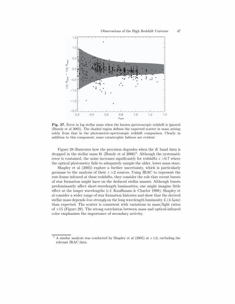
Observations of the High Redshift Universe 47
Fig. 27. Error in log stellar mass when the known spectroscopic redshift is ignored(Bundy et al 2005). The shaded region defines the expected scatter in mass arisingsolely from that in the photometric-spectrosopic redshift comparison. Clearly inaddition to this component, some catastrophic failures are evident.
Figure 28 illustrates how the precision degrades when the K band data isdropped in the stellar mass fit (Bundy et al 2006)5. Although the systematicerror is contained, the noise increases significantly for redshifts z >0.7 wherethe optical photometry fails to adequately sample the older, lower mass stars.
Shapley et al (2005) explore a further uncertainty, which is particularlygermane to the analysis of their z ≃2 sources. Using IRAC to represent therest-frame infrared at these redshifts, they consider the role that recent burstsof star formation might have on the deduced stellar masses. Although burstspredominantly affect short-wavelength luminosities, one might imagine littleeffect at the longer wavelengths (c.f. Kauffmann & Charlot 1998). Shapley etal consider a wider range of star formation histories and show that the derivedstellar mass depends less strongly on the long wavelength luminosity L (4.5µm)than expected. The scatter is consistent with variations in mass/light ratiosof ×15 (Figure 29). The strong correlation between mass and optical-infraredcolor emphasizes the importance of secondary activity.
5 A similar analysis was conducted by Shapley et al (2005) at z ≃2, excluding therelevant IRAC data.

48 Richard S Ellis
Fig. 28. Effect of deriving stellar masses from optical photometry alone (Bundyet al 2006). (Left) Difference in masses derived using BRIK and BRI photometry.(Center) Distribution of uncertainties deduced from Bayesian fitting for the BRIfits. (Right) as center for the BRIK fitting. Although the systematic offset is small,the uncertainty in deduced stellar mass increases dramatically for galaxies withz >0.7.
Fig. 29. Left: Stellar masses versus observed IRAC 4.5µm luminosities for thesample of z ≃2 galaxies studied by Shapley et al (2005). Allowing a wide range ofstar formation histories illustrates a weaker dependence of mass on long wavelengthluminosity than seen in earlier tests at lower redshift based on simpler star formationhistories. The range in rest-frame 1.6µm mass/light ratio is ≃ ×15. (Right) Theexistence of a fairly tight correlation between mass and R −K color demonstratesthe importance of considering secondary bursts of star formation in deriving stellarmasses.

Observations of the High Redshift Universe 49
4.5 Results: Stellar Mass Functions 0< z <1.5
Noting the above uncertainties, we now turn to results compiled from thestellar mass distributions of galaxies undertaken in both spectroscopic andphotometric surveys. A recent discussion of the various results can be foundin Bundy et al (2006).
Brinchmann & Ellis (2000) were the first to address the global evolution ofstellar mass in this redshift range using a morphological sample of 350 galaxieswith spectroscopic redshifts and infrared photometry. The small sample didnot permit consideration of detailed stellar mass functions, but the integratedmass density was partitioned in 3 redshift bins for spheroidals, spirals andirregulars. Surprisingly little growth was seen in the overall mass density fromz ≃1 to today; the strongest evolutionary signal seen is a redistribution ofmass amongst the morphologies dominated by a declining mass density inirregulars with time.
The ratio of the galactic stellar mass Mstar to the current star formationrate SFR, e.g. as deduced spectroscopically or from the rest-frame opticalcolors, is sometimes termed the specific star formation rate, R. This quantityallows us to address the question of whether galaxies have been forming starsfor a significant fraction of the Hubble time, at a rate commensurate withexplaining their assembled mass. A low value for R implies a quiescent objectwhose growth has largely ended; the mean stellar age is quite large. A highvalue of R implies an active object which has assembled recently. A frequently-used alternative is the ‘doubling time’ - that period over which, at the currentSFR, the observed stellar mass would double. This time would be quite shortfor active objects.
Cowie et al (1996), Brinchmann & Ellis (2000), and most recently Juneauet al (2005), found a surprising trend whereby most massive galaxies overz ≃0.5-1.5 are quiescent, having presumably formed their stars well beforez ≃2, whereas low mass galaxies remain surprisingly active. The term ‘down-sizing’ - a signature of continued growth in lower mass galaxies after that inthe high mass galaxies has been completed - was first coined by Cowie etal (1996) and has been used rather loosely in the recent literature to implyany signature of anti-hierarchical activity. In particular, it is important todistinguish between downsizing in star formation activity, which presumablyrepresents some physical process that permits continued star formation inlower mass systems when that in massive galaxies has concluded, from down-
sizing in mass assembly, a truly ‘anti-hierarchical’ process whereby new massis being added to lower mass galaxies at later times (see discussion in Bundyet al 2006).
Before trying to understanding in more detail what causes this mass-dependent star formation, it is worth returning to the issue of dry merg-
ers raised in §4.3. A ‘downsizing’ signature was also seen in the growth ofspheroidal galaxies as analysed by their location on the evolving Fundamen-tal Plane (Treu et al 2005, van der Wel et al 2005). However, van Dokkum

50 Richard S Ellis
(2005) argued that while this may reflect older stars in the more massivegalaxies, the assembled mass may still be young if merging preferentially oc-curs between quiescent objects. The only way to test this hypothesis is todirectly measure the growth rate in spheroidal systems.
Using the deeper and more extensive sample of galaxies available in theGOODS fields, Bundy et al (2005) produced type-dependent stellar mass
functions (Figure 30). Here, for the first time, one can see the morphologicalevolution detected by Brinchmann & Ellis largely arises via the transforma-tion of intermediate mass (≃5. 1010 - 2.1011M⊙) irregulars and spirals intospheroidals. If merging is responsible for this transformation, it is predomi-nantly occurring between gas-rich and active systems even at the very highestmasses. The bulk of the evolution below z ≃1 is simply a redistribution ofstar formation activity, perhaps as a result of mergers or feedback processes.
Interestingly, in Figure 30 there is almost no change in the total massfunction with time above 5. 1010M⊙, suggesting little growth in the massspheroidals that dominate the high mass end. However, it worth rememberingthat the two GOODS fields are limited in size (0.1 deg2) and suffer fromcosmic variance at the 20% level at high redshift increasing to 60% at lowredshift (Bundy et al 2005).
Stellar mass functions for a much larger sample of field galaxies of knownredshift have been analyzed by Bundy et al (2006) utilizing the combinationof extensive spectroscopy and Palomar K-band imaging in four DEEP2 fields(totalling 1.5 deg2). This sample has the benefit of being much less affectedby cosmic variance although, as there is no complete coverage with HST, mor-phological classifications are not possible. Color bimodality has been analyzedin the DEEP2 sample (Weiner et al 2005) and Bundy et al use the rest-frameU − B color and spectroscopic [O II] equivalent width to separate quiescentand active galaxies.
Figure 31 shows a direct comparison of the integrated stellar mass func-tions from this large survey alongside other, less extensive surveys, most ofwhich are based only on photometric redshifts. Although each is variance lim-ited in different ways, one is struck again by the quite modest changes in theabundance of massive galaxies since z ≃1.
Next we consider (Figure 32) the stellar mass functions for the quiescentand active star-forming galaxies independently, partitioned according to therest-frame U−B color. The surprising result here is the existence of a thresholdor quenching mass, MQ above which there are no active systems. This isimplied independently in Figure 30 where, within the redshift bin 0.55 < z <0.8, there are no spirals or irregulars with mass > 1011M⊙. Interestingly, thereis also a modest downward transition in MQ with time.
A remarkably consistent picture emerges from these studies. Over the red-shift range 0< z <1.5, the stellar mass function has changed very little atthe high mass end. Substantial growth, in terms of a mass doubling on ≃5-8Gyr timescale, is only possible for galaxies with stellar masses below 1010M⊙.Above this mass, the basic evolutionary signal is a quenching of star forma-
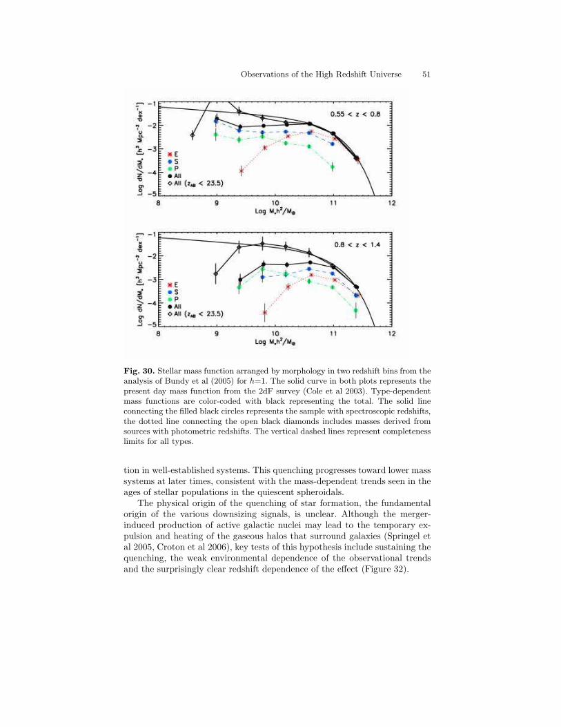
Observations of the High Redshift Universe 51
Fig. 30. Stellar mass function arranged by morphology in two redshift bins from theanalysis of Bundy et al (2005) for h=1. The solid curve in both plots represents thepresent day mass function from the 2dF survey (Cole et al 2003). Type-dependentmass functions are color-coded with black representing the total. The solid lineconnecting the filled black circles represents the sample with spectroscopic redshifts,the dotted line connecting the open black diamonds includes masses derived fromsources with photometric redshifts. The vertical dashed lines represent completenesslimits for all types.
tion in well-established systems. This quenching progresses toward lower masssystems at later times, consistent with the mass-dependent trends seen in theages of stellar populations in the quiescent spheroidals.
The physical origin of the quenching of star formation, the fundamentalorigin of the various downsizing signals, is unclear. Although the merger-induced production of active galactic nuclei may lead to the temporary ex-pulsion and heating of the gaseous halos that surround galaxies (Springel etal 2005, Croton et al 2006), key tests of this hypothesis include sustaining thequenching, the weak environmental dependence of the observational trendsand the surprisingly clear redshift dependence of the effect (Figure 32).

52 Richard S Ellis
Fig. 31. The evolving stellar mass function from the comparison of Bundy et al(2006).
4.6 Results: Stellar Mass Functions z>1.5
With current facilities, the stellar mass data beyond z ≃1.5 generally probesonly the higher mass end of the distribution and relies on photometric ratherthan spectroscopic data. Nonetheless, the results emerging have received asmuch attention as those at lower redshift. Unlike the complexities of under-standing downsizing and the redistribution of mass and morphology in thez <1 data, the basic question at stake here is simply whether the abundance
of massive z ≃2 galaxies is larger than expected in the standard model.Testing the decline with redshift in the comoving abundance of, say, sys-
tems with stellar mass greater than 1011M⊙, expected in ΛCDM has been afrustrating story for the observers for two reasons. Firstly, the most massivesystems are rare and clustered, and so determining reliable density estimatesbeyond z ≃1.5 has required panoramic deep infrared data which has only re-

Observations of the High Redshift Universe 53
Fig. 32. The evolving stellar mass function split into quiescent (red) and active(blue) sources from the survey of Bundy et al (2006). Uncertainties arising fromcounting statistics and errors in the stellar masses are indicated by the associatedshading. The thin solid line represents the local 2dF function (Cole et al 2003) andthe dark and light grey regions represent total mass functions using only spectro-scopic and including photometric redshifts respectively.
cently arrived. For a review of the early observational efforts see Benson, Ellis& Menanteau (2002)
Secondly, there has been considerable confusion in the theoretical litera-ture on the expected rate of decline in > 1011M⊙ systems. Early predictions(Kauffmann, Charlot & White 1996) claimed a 3-fold decline in the comovingabundance to z ≃1 in apparent agreement with the large photometric sampleanalyzed by Bell et al (2004). However, careful comparisons of independentsemi-analytical predictions (Kauffmann et al 1999, Cole et al 2000) revealsubstantial differences (by an order of magnitude for the same world model)in the rate of decline even to z ≃1 (Benson, Ellis & Menanteau 2002). In re-

54 Richard S Ellis
ality, the predictions depend on many parameters where differences can havea large effect for the region of the mass function where the slope dN / dM issteep.
Dickinson et al (2003) undertook a pioneering study to evaluate the growthof stellar mass with photometric redshift using deep H <26.5 NICMOS datain the Hubble Deep Field North. Although a tiny field (5 arcmin2), the workwas the first to demonstrate the existence of 1011M⊙ galaxies at z ≃1.5-2as well as the challenges of estimating reliable abundances. A similar HDF-Sanalysis was undertaken by Rudnick et al (2003).
A more representative area of 4×30 arcmin was probed spectroscopicallyin the Gemini Deep Deep Survey (Glazebrook et al 2004), albeit to a muchshallower depth. These authors claimed a ‘surprising’ abundance of 1011M⊙
systems to z ≃2. Although an absolute comparison of the abundances withsemi-analytical predictions is not likely to be illuminating for the reasonsmentioned above, the redshift-dependent mass growth rate over 1< z <2,derived empirically from both the stellar masses and the integrated star for-mation rate, seems much slower than expected in the semi-analytical models(Granato et al 2000). Of particular interest is the fact that the mass growthrate seems not depend strongly on the mass range in question in apparentdisagreement with the model predictions (Figure 33).
Although many of the observers associated with the Gemini Deep DeepSurvey have claimed the abundance and slow growth rate of massive galaxiesover 1.5< z <2 poses a crisis for the standard model, alongside the puzzling‘anti-hierarchical’ behavior observed for z <1.5, the plain fact is that there isconsiderable uncertainty in the semi-analytical predictions.
4.7 Quiescent Galaxies with 2< z <3
Finally, it is illustrative to consider the dramatic effect that infrared datafrom panoramic ground-based cameras and the Spitzer Space Telescope ishaving, not only on our knowledge of the distribution of stellar masses athigh redshift, but also how stellar mass is distributed among quiescent andstar-forming populations. Until recently, there was widespread belief that thebulk of the star formation in this era, and probably a significant fraction of thestellar mass, lay in the Lyman break population. By contrast, van Dokkumet al (2006) have examined the rest-frame U − V colors of a sample of 300> 1011M⊙ galaxies with 2< zphoto < 3 (Figure 34) and claim almost 80%are quiescent. The definition of ‘quiescent’ here is somewhat important toget correct, given it now emerges that many of the originally-selected distantred galaxies with J −K >2.3 (§2.6) turn out to have quite respectable starformation rates. Infrared spectroscopy sensitive to Hα emission and the 4000Abreak is making great strides in clarifying this question (Kriek et al 2006).

Observations of the High Redshift Universe 55
Fig. 33. The mass assembly history derived from stellar masses in the GeminiDeep Deep spectroscopic survey (Glazebrook et al 2004). Colored data points referto observed cumulative densities ρ (> M) for various mass ranges and the greenshaded region to estimates derived from the integrated star formation history. Thecolored lines refer to predicted growth rates according to the GALFORM semi-analytic models.
Fig. 34. The distribution of rest-frame U-V color for a Spitzer-selected sample of2 < z <3 galaxies with stellar masses > 1011 M⊙ from the analysis of van Dokkumet al (2006). Almost 80% of this sample in a quiescent state consistent with havingcompleted the bulk of their assembly.

56 Richard S Ellis
4.8 Lecture Summary
In this lecture we have demonstrated important new techniques for estimatingthe stellar masses of all types of galaxies to impressive high redshift (z ≃3).The reliability of these techniques is improved greatly by having spectro-scopic, rather than photometric, redshifts and, for z > 0.7, by the additionof infrared photometry. These techniques augment and extend more precisemeasures available for restricted classes of galaxies - such as the FundamentalPlane for pressure-supported spheroidals, and the Tully-Fisher relationshipfor rotationally-supported disks.
These various probes point to a self-consistent, but puzzling, descriptionof mass assembly since z ≃1.5. During this era, massive galaxies have hardlygrown at all - most of the star formation and rapid growth is occurring insystems whose masses are less than 1010M⊙. Remarkably, the star formationappears to be quenched above a certain threshold mass whose value, in turn,is declining with time.
Energetic sources such as supernovae or active nuclei may be responsi-ble for this ‘downsizing’ signature but further work is needed to verify boththe weak environmental trends seen in the observations and the redshift-dependent trends in the threshold mass.
Beyond z ≃1.5, the number and distribution of massive (> 1011M⊙ galax-ies has led to some surprises. Although the sheer abundance may not be aproblem for contemporary models, the fact that so many have apparently com-pleted their star formation is more challenging and consistent with the slowgrowth rate observed at later times. The observational situation is rapidlydeveloping but consistent with the presence of a surprisingly abundant andmature population of massive galaxies by z ≃3.

Observations of the High Redshift Universe 57
5 Witnessing the End of Cosmic Reionization
5.1 Introduction - Some Weighty Questions
We now turn to the exciting and rapidly developing area of understandingcosmic reionization. This event, which marks the end of the so-called ‘DarkAges’ when the intergalactic medium became transparent to ultraviolet pho-tons, was a landmark in cosmic history. In some ways the event might beconsidered as important as the epoch of recombination which isolates the for-mation of the hydrogen atom, or the asssociated surface of last scatteringwhen photons and baryonic matter decouple. In the case of the era of cosmicreionization, although we cannot yet be sure, many believe we are isolatingthat period when the first sources had sufficient output to contribute to theenergy balance of the intergalactic medium. Even though some early lumi-nous forerunners might be present, the epoch of reionization can be directlyconnected with cosmic dawn for starlight.
It seems an impossible task to give an authoritative observational accountof how to probe this era. So many issues are complete imponderables! Whendid reionization occur? Was it a gradual event made possible by a complextime sequence of sources, or was there a spectacular synchronized moment?Can we conceive of an initial event, followed by recombination and a secondphase?
What were the sources responsible? History has shown the naivety of as-tronomers in assuming a single population to be responsible for various phe-nomena - usually some complex combination is the answer. And, perhaps mostambitiously, what is the precise process by which photons escape the sourcesand create ionized regions?
Four independent observational methods are helpful in constraining theredshift range where we might search for answers to the above questions. Inthis lecture, we will explore how these work and the current (and rapidlychanging) constraints they offer. These are:
• Evolution in the optical depth of Lyman series absorption lines in highredshift quasars (Fan et al 2006a,b). Although QSOs are only found toredshifts of z ≃6.5, high quality spectroscopic data gives us a glimpse ofa potential change in the degree of neutrality of the IGM beyond z ≃5.5such as might be expected if reionization was just ending at that epoch.
• The ubiquity of metal absorption lines in the IGM as probed again byvarious spectra of the highest redshift QSOs. Carbon, in particular, isonly produced in stellar nuclei and its presence in all sightlines to z ≃5-6 (Songaila 2004) is highly indicative of a widespread process of earlierenrichment from the first generation of supernovae.
• The large angular scale power in the temperature - polarization cross-correlation function seen in the microwave background (Kogut et al 2003,

58 Richard S Ellis
Spergel et al 2006). This signal is produced by electron scattering fore-ground to the CMB. Depending on models of large scale structure, the op-tical depth of scattering gives some indication of the redshift range wherethe ionized particles lie.
• The stellar mass density in assembled sources at redshifts z ≃5-6, about 1billion years after the Big Bang, as probed by the remarkable combinationof HST and Spitzer (Stark & Ellis 2005, Stark et al 2006a, Yan et al 2006,Eyles et al 2006). A census of the mass in stars must be the integral ofpast activity which can be compared with that necessary to reionize theUniverse.
5.2 The Gunn-Peterson Test and SDSS QSOs
In a remarkable paper, long before QSOs were located at redshifts beyond2.5, James Gunn and Bruce Peterson realized (Gunn & Peterson 1965) thatthe absence of broad troughs of hydrogen absorption in the spectra of QSOsmust indicate intergalactic hydrogen is ionized. They postulated a future testwhereby the spectra of QSOs of successively higher redshift would be scruti-nized to locate that epoch when the IGM was neutral.
For an optical spectrum, redshifted to reveal that portion of the rest-frameUV shortward of the Lyman α emission line of the QSO itself (λ 1216 A ), therelative transmission T is defined as
T = f(λ) / fcont
where fcont represents the continuum radiation from the QSOs. The trans-mission is reduced by Lyman α absorption in any foreground (lower redshift)clouds of neutral hydrogen whose Gunn-Peterson opacity is then
τGP = −ln T
The first ‘complete troughs’ in the absorption line spectra of distant QSOwere presented by Becker et al (2001) and Djorgovski et al (2001) and a morecomprehensive sampling of 11 SDSS QSOs was presented by Fan et al (2003).Recently, an analysis of 19 5.74< z <6.42 QSOs was presented by Fan et al(2006b).
Figure 35 illustrates how absorption structures along the same line of sightcan be independently probed using Lyman α and higher order lines such asLyman β.
To understand how this is effective, in a uniform medium τGP is relatedto the abundance of absorbing neutral hydrogen atoms by the following ex-pression:
τGP =πe2
mecfα λαH
−1(z)nHI
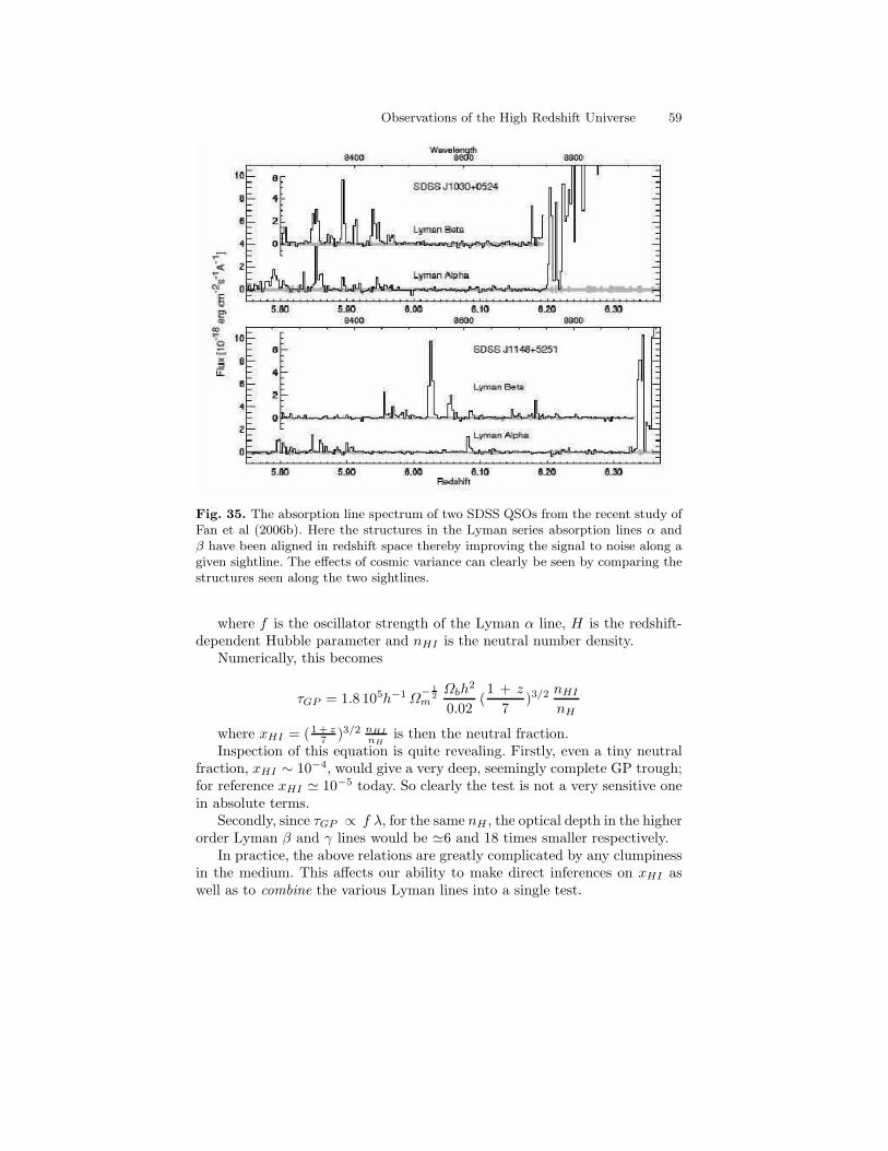
Observations of the High Redshift Universe 59
Fig. 35. The absorption line spectrum of two SDSS QSOs from the recent study ofFan et al (2006b). Here the structures in the Lyman series absorption lines α andβ have been aligned in redshift space thereby improving the signal to noise along agiven sightline. The effects of cosmic variance can clearly be seen by comparing thestructures seen along the two sightlines.
where f is the oscillator strength of the Lyman α line, H is the redshift-dependent Hubble parameter and nHI is the neutral number density.
Numerically, this becomes
τGP = 1.8 105h−1Ω−
1
2
mΩbh
2
0.02(1 + z
7)3/2 nHI
nH
where xHI = (1+ z7 )3/2 nHI
nH
is then the neutral fraction.Inspection of this equation is quite revealing. Firstly, even a tiny neutral
fraction, xHI ∼ 10−4, would give a very deep, seemingly complete GP trough;for reference xHI ≃ 10−5 today. So clearly the test is not a very sensitive onein absolute terms.
Secondly, since τGP ∝ f λ, for the same nH , the optical depth in the higherorder Lyman β and γ lines would be ≃6 and 18 times smaller respectively.
In practice, the above relations are greatly complicated by any clumpinessin the medium. This affects our ability to make direct inferences on xHI aswell as to combine the various Lyman lines into a single test.

60 Richard S Ellis
Instead, workers have examine the relative distribution of τGP with red-shift independently from the various Lyman series absorption statistics. Anincrease in τGP with redshift could just be a natural thickening of the Lymanabsorption forest and, given its weak connection with xHI , not imply anythingprofound about cosmic reionization. However, if it can be shown empiricallythat the various diagnostics show a discontinuity in the xHI -redshift trends,conceivably we are approaching the neutral era.
Figure 36 shows that for z <5.5, τ ∝ (1+z5 )4.3 for both the Lyα and
Lyβ forests to reasonable precision. However, beyond z ≃5.5, both redshifttrends are much steeper, ∝ (1 + z)11. The dispersion around the trends alsoincreases significantly at higher redshift. Taken together, both results suggest aqualitative change in nature of the IGM beyond z ≃5.5 (but for an alternativeexplanation see Becker et al 2006).
Fig. 36. Evolution in the Gunn-Peterson optical depth, τ , for both the Lyman α(left) and β (right) forests from the distant SDSS QSO analysis of Fan et al (2006.The dotted lines represent fits to the data for zabs <5.5, beyond which there isevidence in both species for an upturn in the opacity of the intergalactic medium.
Fan et al (2006a,b) discuss several further probes of the nature of theIGM at z ≃6. One relates to the proximity effect - the region around eachQSO where it is clear from the spectrum that the IGM is being ionized bythe QSO itself. Although this region is excluded in the analyses above, theextent of this region contains valuable information on the nature of the IGM.It appears that the radius of the region affected, R is less at higher redshiftaccording to R ∝ [(1 + z)xHI ]−1/3 suggesting that the most distant QSOs inthe sample (z ≃6.5) lie in a IGM whose neutral fraction is ≃14 times higherthan those at z ≃5.7.
Another valuable measure is how the regions of complete absorption, theso-called ‘dark gaps’ in the spectrum where transmission is effectively zero,are distributed. Fan et al define a ‘gap’ as a contiguous region in redshiftspace where τ >3.5. The distribution of gaps contains some information on

Observations of the High Redshift Universe 61
the topology of reionization. We would expect regions of high transmissionto be associated with large HII regions, centered on luminous star-formingsources. The dark gaps increase in extent from ≃10 to 80 comoving Mpc overthe redshift range samples suggesting the IGM is still not neutral at z ≃6.5.Although the Gunn-Peterson and gap statistics make similar statements aboutreionization, suggesting the neutral fraction at z ≃6.2 is 1-4%, Fan et alconsider that beyond z ≃6.5, gap statistics will become a more powerful probe.This is because the redshift distribution of those few spectroscopic pixelswhere the transmission is non-zero will become the only effective signal.
5.3 Metallicity of the High Redshift IGM
A second measure of the redshift range of early star formation is containedin the properties of the CIV forest observed in the spectra of high redshiftQSOs (Songaila 2005, 2006). Carbon is only produced in stellar nuclei (it isnot produced in the hot Big Bang) and so the ubiquity of CIV along manysightlines to z ≃5-6 QSOs is a powerful argument for early enrichment.
CIV was seen in the Lyα forest in 1995 (Cowie et al 1995) with N(CIV)/N(HI)∼10−2 to 10−3. However, it was subsequently seen in even the weakest Lyαsystems (Ellison et al 2000). This is a particularly powerful point since itargues that enrichment is not confined to localized regions of high columndensity but is generic to the intergalactic medium as a whole (Figure 37)
A quantitative interpretation of the CIV abundance, in terms of how muchearly star formation occurred earlier than the highest redshift probed, relies onlocating a ‘floor’ in the abundance-redshift relation. Unfortunately, the actualobserved trend, measured via the contribution of the ion to the mass densityΩ(CIV ) from z ≃5 to 2, does not seem to behave in the manner expected. Forexample, there is no strong rise in the CIV abundance to lower redshift de-spite the obvious continued star formation that occurred within these epochs(Songaila 2006, Figure 38). This is a major puzzle (c.f. Oppenheimer et al2006).
5.4 Linear Polarization in the WMAP Data
In 2003, the WMAP team (Kogut et al 2003) presented the temperature-polarization cross angular power spectrum from the first year’s data andlocated a 4σ non-zero signal at very low multipoles (l <8) which they in-terpreted in terms of foreground electron scattering of microwave backgroundphotons with an optical depth τe = 0.17 ± 0.04 corresponding to ionizedstructures at zreion ≃20 (Figure 39a). The inferred redshift range dependssensitively on the history of the reionization process. Bennett et al (2003) ar-gued that if reionization occurred instantaneously it corresponds to a redshiftzreion ≃ 17 ± 5, whereas adopting a more reasonable Press-Schechter formal-ism and an illustrative cooling and enrichment model, Fukugita & Kawasaki

62 Richard S Ellis
Fig. 37. (Left) Keck ESI absorption line spectrum of the z=4.5 QSO BR2237-0607from the study of Songaila (2005). A sparsely populated CIV forest from 7500-8500A accompanies the dense Lyα forest seen below 6800 A . (Right) Distributionof column densities of CIV absorbers per unit redshift interval in Q1422+231 fromthe survey of Ellison et al (2000).
(2003) demonstrated that the same signal can be interpreted with a delayedreionization occurring at zreion ≃9-10.
Just before the Saas-Fee lectures, the long-awaited third year WMAP datawas published (Spergel et al 2006). A refined analysis significantly loweredboth the normalization of the dark matter power spectrum to σ8 = 0.74 ±0.05, and the optical depth to electron scattering to τe = 0.09 ± 0.03. Thesame model of instantaneous reionization reduces the corresponding redshiftto zreion = 11 ± 3(2σ) - a significant shift from the 1 year data.
To illustrate the uncertainties, Spergel et al introduce a more realistichistory of reionization via the ionization fraction xe. Suppose above zreion,

Observations of the High Redshift Universe 63
Fig. 38. Modest evolution in the contribution of intergalactic CIV and SIV over2< z <5 as measured in terms of the ionic contribution to the mass density, Ω(Songaila 2005).
xe ≡ 0 and below z=7, xe ≡ 1. Then suppose zreion is defined as that in-termediate point when xe = x0
e for 7< z < zreion. Figure 39b illustrates theremarkable insensitivity of zreion to the adopted value of x0
e for x0e <0.5. De-
spite improved data, the redshift range implied by the WMAP data spans thefull range 10< z <20.
5.5 Stellar Mass Density at z ≃5-6
Neither the Gunn-Peterson test nor the WMAP polarization data necessarilydemonstrate that reionization was caused by early star-forming sources; bothonly provide constraints on when the intergalactic medium was first reionized.The CIV test is a valuable complement since it provides a measure of earlyenrichment which can only come from star-forming sources. Unfortunately,powerful though the ubiquitous presence of CIV is in this context, as wehave seen, quantitative constraints are hard to derive. We thus seek a furtherconstraint on the amount of early star formation that might have occurred.
In Lecture 4 we introduced the techniques astronomers are now using toderive stellar masses for distant galaxies. Although the techniques remainapproximate, it must follow that the stellar mass density at a given epochrepresents the integral over time and volume of the past star formation. In-deed, we already saw a successful application of this in reconciling past starformation with the local stellar mass density observed by 2dF (Figure 21).Specifically, at a particular redshift, z

64 Richard S Ellis
Fig. 39. (Left) The 4σ detection of reionization via an excess signal at large scalesin the angular cross correlation power spectrum of the temperature and polariza-tion data in the first year WMAP data (Kogut et al 2003). (Right) Constraints onthe redshift of reionization, zreion, from the third year WMAP data (Spergel et al2006). The contours illustrate how the zreion inferred from the lowered optical depthdepends on the history of the ionized fraction xe(z), see text for details.
M∗ =
∫ z
∞
ρ∗(z) dV (z)
Using the techniques described in Lecture 4, stellar mass estimates havebecome available for some very high redshift galaxies detected by Spitzer(Eyles et al 2005, Mobasher et al 2005, Yan et al 2005). For the most lumi-nous Lyman ‘dropouts’, these estimates are quite substantial, some exceeding1011M⊙ implying much earlier activity. Recently, several groups (Stark et al2006a, Yan et al 2006, Eyles et al 2006) have been motivated to provide thefirst crude estimates on the volume averaged stellar mass density at theseearly epochs. Part of this motivation is to check whether the massive galaxiesseen at such high redshift can be reconciled with hierarchical theory, but asStark & Ellis (2005) proposed, the established stellar mass can also be usedto probe earlier star formation and its likely impact upon cosmic reionization.
A very relevant question is whether the observed mass density at z ≃5-6is greater than can be accounted for by the observed previous star formationhistory. We will review the rather uncertain data on the star formation densityρ∗(z) beyond z ≃6 in the next Lecture. However, Stark et al (2006a) find thateven taking a reasonably optimistic measure of ρ∗(z) from recent compilationsby Bouwens et al (2006) and Bunker et al (2006), it is hard to account for thestellar mass density at z ≃5 (Figure 40).
There are currently two major limitations in this comparison. First, mostof the v- and i-drops are located photometrically; even a small degree of con-tamination from lower redshift galaxies could upward bias the stellar massdensity. On the other hand only star-forming galaxies are located by the Ly-man break technique so this bias could easily be offset if there are systems in

Observations of the High Redshift Universe 65
Fig. 40. A comparison of the assembly history of stellar mass inferred from theobserved decline in star formation history to z ≃10 (solid line) with extant dataon the stellar mass density at z ≃5 and 6 (data points from Stark et al 2006a,Yan et al 2006, Eyles et al 2006). Different estimates at a given redshift representlower limits based on spectroscopically-confirmed and photometric redshift samples.The red line shows the growth in stellar mass expected from the presently-observedluminous star forming galaxies; a shortfall is observed. The blue dotted line showsthe improvement possible when a dominant component of high z lower luminositysystems is included.
a quiescent state as evidenced by the prominent Balmer breaks seen in manyof the Spitzer-detected sources (Eyles et al 2005, 2006). This limitation willultimately be overcome with more careful selection methods and deeper spec-troscopy. Secondly, and more profoundly, the precision of the stellar massesmay not be up to this comparison. Much has to be assumed about the natureof the stellar populations involved which may, quite reasonably, be somewhatdifferent from those studied locally. The discrepancy noted by Stark et al isonly a factor of ×2-3, possibly within the range of uncertainty.
Regardless, if this mismatch is reinforced by better data, the implicationsare very interesting in the context of reionization. It could mean early star-forming systems are extincted, lie beyond z ≃10 where current searches end, orperhaps most likely that early star formation is dominated by lower luminositysystems (Figure 40). By refining this technique and using diagnostics such asthe strength of the tell-tale Balmer break, it may ultimately be possible to
66 Richard S Ellis
age-date the earlier activity and compare its efficacy with that required toreionize the Universe.
5.6 Lecture Summary
In this lecture we have introduced four very different and independent probesof cosmic reionization, each of which suggests star formation activity mayextend well into the redshift range 6< z < 20. Two of these probes rely ona contribution from early star formation (the metallicity of the intergalacticmedium and the assembled stellar mass density at z ≃5-6).
The earliest result was the presence of neutral hydrogen troughs in thespectra of distant QSOs. Although the arguments for reionization ending atz ≃6 seem compelling at first sight, they ultimately rely on an empirically-deduced transition in the changes in the opacity of the Lyα and Lyβ linebelow and above z ≃5.5.
The second result - the ubiquity of carbon in even the weakest absorbingclouds at z ≃5 is firm evidence for early star formation. However, it seems hardto locate the high redshift ‘abundance floor’ and hence to quantify whetherthis early activity is sufficient for reionization. Indeed, a major puzzle is thelack of growth in the carbon abundance over the redshift range where galaxiesare assembling the bulk of their stars.
The WMAP polarizations results have received the most attention, mainlybecause the first year data indicated a surprisingly large optical depth and ahigh redshift for reionization. However, there were some technical limitationsin the original analysis and it now seems clear that the constraints on theredshift range when the foreground polarization is produced are not verytight.
Finally, an emerging and very promising technique is simply the census ofearly star formation activity as probed by the stellar masses (and ages) of themost luminous dropouts at z ≃5-6. Although significant uncertaintes remain,the prospects for improving these constraints are good and, at this moment,it seems there must have been quite a significant amount of early (z >6) starformation activity, quite possibly in low luminosity precursors.

Observations of the High Redshift Universe 67
6 Into the Dark Ages: Lyman Dropouts
6.1 Motivation
Surveys of galaxies at and beyond a redshift z ≃6 represent the current ob-servational frontier. We are motivated to search to conduct a census of theearliest galaxies seen 1 Gyr after the Big Bang as well as to evaluate the con-tribution of early star formation to cosmic reionization. Although impressivefuture facilities such as the next generation of extremely large telescope6 andthe James Webb Space Telescope (Gardner et al 2006) are destined to addressthese issues in considerable detail, any information we can glean on the abun-dance, luminosity and characteristics of distant sources will assist in planningtheir effective use.
In this lecture and the next, we will review the current optical and near-infrared techniques for surveying this largely uncharted region. They include
• Lyman dropouts: photometric searches based on locating the rest-frameultraviolet continuum of star-forming sources introduced in Lecture 3. Thekey issue here is reducing contamination from foreground sources sincemost sources selected via this technique are too faint for confirmatoryspectroscopy.
• Lyman alpha emitters: spectroscopic or narrow-band searches for sourceswith intense Lyα emission. As the line is resonantly-scattered by neutralhydrogen its profile and strength gives additional information on the stateof the high redshift intergalactic medium.
• Strong gravitational lensing: by coupling both above techniques with themagnification afforded by lensing clusters, it is possible to search for lowerluminosity sources at high redshift. Since the magnified areas are small,the technique is only advantageous if the luminosity function has a steepfaint end slope.
For the Lyman dropouts discussed here, as introduced in the last lecture,there is an increasingly important role played by the Spitzer Space Telescopein estimating stellar masses and earlier star formation histories.
The key questions we will address in this lecture focus on the (somewhatcontroversial) conclusions drawn from the analyses of Lyman dropouts thusfar, namely:
1. How effective are the various high z selection methods? The characteris-tic luminosity L∗ at z ≃6 corresponds to iAB ≃26 where spectroscopicsamples are inevitably biased to those with prominent Lyα emission. Ac-cordingly there is great reliance on photometric redshifts and a real dangerof substantial contamination by foreground red galaxies and Galactic coolstars.
6 e.g. The US-Canadian Thirty Meter Telescope - http//www.tmt.org

68 Richard S Ellis
2. Is there a decline in the UV luminosity density, ρUV , over the range 3<z <6? The early results were in some disagreement. Key issues relate tothe degree of foreground contamination and cosmic variance in the verysmall deep fields being examined.
3. Is the observed UV density, ρUV , at z ≃6 sufficient to account for reion-ization? The answer depends on the contribution from the faint end of theluminosity function and whether the UV continuum slope is steeper thanpredicted for a normal solar-metallicity population.
4. Significant stellar masses have been determined for several z ≃6 galaxies.Are these in conflict with hierarchical structure formation models?
6.2 Contamination in z ≃6 Dropout Samples
The traditional dropout technique exploited very effectively at z ≃3 (Lecture3) is poorly suited for z ≃6 samples because the use of a simple i−z > 1.5 colorcut still permits significant contamination by passive galaxies at z ≃2 andGalactic stars. The addition of an optical-infrared color allows some measureof discrimination (Stanway et al 2005) since a passive z ≃2 galaxy will bered over a wide range in wavelength, whereas a star-forming z ≃6 galaxyshould be relatively blue in the optical-infrared color corresponding to its rest-frame ultraviolet (Figure 41). Application of this two color technique suggestscontamination by foreground galaxies is ≃10% at the bright end (zAB <25.6)but negligible at the UDF limit (zAB <28.5)
Unfortunately, the spectral properties of cool Galactic L dwarfs are dom-inated by prominent molecular bands rather than simply by their effectivetemperature. This means that they cannot be separated from z ≃6 galaxiesin a similar color-color diagram. Indeed, annoyingly, these dwarfs occupy pre-cisely the location of the wanted z ≃6 galaxies (Figure 42)! The only practicalway to discriminate L dwarfs is either via spectroscopy or their unresolvednature in ACS images.
Stanway et al (2004) conducted the first comprehensive spectroscopic andACS imaging survey of a GOODS i-drop sample limited at zAB <25.6, findingthat stellar contamination at the bright end of the luminosity function of atraditional (iAB − zAB >1.5) color cut could be as high as 30-40%. Unfortu-nately, even with substantial 6-8 hour integrations on the Keck telescope, red-shift verification of the distant population was only possible in those dropoutcandidates with Lyα emission. Stanway et al (2005) subsequently analyzed theACS imaging properties of a fainter subset arguing that stellar contaminationdecreases with increasing apparent magnitude.
Further progress has been possible via the use of the ACS grism on boardHST (Malhotra et al 2005). As the OH background is eliminated in space,despite its low resolution, it is possible even in the fairly low signal/noise dataachievable with the modest 2.5m aperture of HST to separate a Lyman breakfrom a stellar molecular band. It is claimed that of 29 zAB <27.5 candidateswith (i-z)>0.9, only 6 are likely to be low redshift interlopers.

Observations of the High Redshift Universe 69
Fig. 41. The combination of a i− z and z − J color cut permits the distinction ofz ≃5.7-6.5 star forming and z ≃2 passive galaxies. Both may satisfy the i− z >1.5dropout selector, but the former should lie blueward of the z−J=1.0 divider, whereasz ≃2 are red in both colors. Crosses represent the location of candidates in theGOODS field and model tracks illlustrate the predicted colors for typical SEDsobserved at the respective redshifts (Stanway et al 2005).
Regrettably, as a result of these difficulties, it has become routine to relyentirely on photometric and angular size information without questioning fur-ther the degree of contamination. This is likely one reason why there remainsignificant discrepancies between independent assessments of the abundanceof z ≃6 galaxies (Giavalisco et al 2004, Bouwens et al 2004, Bunker et al 2004).Although there are indications from the tests of Stanway et al (2004, 2005)and Malhotra et al (2005) that contamination is significant only at the brightend, the lack of a comprehensive understanding of stellar and foreground con-tamination remains a major uncertainty.
6.3 Cosmic Variance
The deepest data that has been searched for i-band dropouts includes the twoGOODS fields (Dickinson et al 2004) and the Hubble Ultra Deep Field (UDF,

70 Richard S Ellis
Fig. 42. (Left) Keck spectroscopic verification of two contaminating L dwarfs lyingwithin the GOODS i− z dropout sample but pinpointed as likely to be stellar fromACS imaging data. The smoothed spectra represent high signal to noise brighterexamples for comparison purposes. Strong molecular bands clearly mimic the Ly-man dropout signature. (Right) Optical-infrared color diagram with the dropoutcolor selector, iAB − zAB > 1.5, shown as the vertical dotted line. Bright L dwarfs(lozenges) frustratingly occupy a similar region of color space as the z ≃6 candidates(points with error bars) (Stanway et al 2004).
Beckwith et al 2006). As these represent publicly-available fields they havebeen analyzed by many groups to various flux limits. The Bunker/Stanwayteam probed the GOODS fields to zAB=25.6 (spectroscopically) and 27.0(photometrically, and the UDF to zAB=28.5. At these limits, it is instructiveto consider the comoving cosmic volumes available in each field within theredshift range selected by the typical dropout criteria. For both GOODS-N/Sfields, the total volume is ≃5. 105 Mpc3, whereas for the UDF it is only 2.6104 Mpc3. These contrast with 106 Mpc3 for a single deep pointing taken withthe SuPrime Camera on the Subaru 8m telescope.
Somerville et al (2004) present a formalism for estimating, for any popula-tion, the fractional uncertainty in the inferred number density from a surveyof finite volume and angular extent. When the clustering signal is measurable,the cosmic variance can readily be calculated analytically. However, for fron-tier studies such as the i-dropouts, this is not the case. Here Somerville et alpropose to estimate cosmic variance by appealing to the likely halo abundancefor the given observed density using this to predict the clustering accordingto CDM models. In this way, the uncertainties in the inferred abundance ofi-dropouts in the combined GOODS fields could be ≃20-25% whereas that inthe UDF could be as high as 40-50%.

Observations of the High Redshift Universe 71
It seems these estimates of cosmic variance can only be strict lower limitsto the actual fluctuations since Somerville et al make the assumption thathalos containing star forming sources are visible at all times. If, for example,there is intermittent activity with some duty cycle whose ”on/off” fraction isf , the cosmic variance will be underestimated by that factor f (Stark et al,in prep).
6.4 Evolution in the UV Luminosity Density 3< z <10?
The complementary survey depths means that combined studies of GOODSand UDF have been very effective in probing the shape of the UV luminosityfunction (LF) at z ≃67. Even so, there has been a surprising variation inthe derived faint end slope α. Bunker et al (2004) claim their data (54 i-dropouts) is consistent with the modestly-steep α=-1.6 found in the z ≃3Lyman break samples (Steidel et 2003), whereas Yan & Windhorst (2004)extend the UDF counts to zAB=30.0 and, based on 108 candidates, find α=-1.9, a value close to a divergent function! Issues of sample completeness arecentral to understanding whether the LF is this steep.
In a comprehensive analysis based on all the extant deep data, Bouwens etal (2006) have attempted to summarize the decline in rest-frame UV luminos-ity density over 3< z <10 as a function of luminosity (Figure 43). They at-tribute the earlier discrepancies noted between Giavalisco et al (2004), Bunkeret al (2004) and Bouwens et al (2004) to a mixture of cosmic variance and dif-ferences in contamination and photometric selection. Interestingly, they claima luminosity-dependent trend in the sense that the bulk of the decline occursin the abundance of luminous dropouts, which they attribute to hierarchicalgrowth.
A similar trend is seen in ground-based data obtained with Subaru. Al-though HST offers superior photometry and resolution which is effective ineliminating stellar contamination, the prime focus imager on Subaru has amuch larger field of view so that each deep exposure covers a field twice aslarge as both GOODS N+S. As they do not have access to ACS data over suchwide fields, the Japanese astronomers have approached the question of stellarcontamination in an imaginative way. Shioya et al (2005) used two interme-diate band filters at 709nm and 826nm to estimate stellar contamination inboth z ≃5 and z ≃6 broad-band dropout samples. By considering the slope
of the continuum inbetween these two intermediate bands, in addition to astandard i − z criterion, they claim an ability to separate L and T dwards.In a similar, but independent, study, Shimasaku et al (2005) split the z bandinto two intermediate filters thereby measuring the rest-frame UV slope justredward of the Lyman discontinuity. These studies confirm both the redshiftdecline and, to a lesser extent, the luminosity-dependent trends seen in theHST data.7 In this section we will only refer to the observed (extincted) LFs and luminosity
density

72 Richard S Ellis
Fig. 43. Evolution in the rest-frame UV (1350 A ) luminosity density (right ordi-nate) and inferred star formation rate density ignoring extinction (left ordinate) fordrop-out samples in two luminosity ranges from the compilation by Bouwens et al(2006). A marked decline is seen over 3 < z < 6 in the contribution of luminoussources.
Although it seems there is a 5× abundance decline in luminous UV emit-ting galaxies from z ≃3 to 6, it’s worth noting again that the relevant countsrefer to sources uncorrected for extinction. This is appropriate in evaluatingthe contribution of UV sources to the reionization process but not equivalent,necessarily, to a decline in the star formation rate density. Moreover, althoughthe luminosity dependence seems similar in both ground and HST-based sam-ples, it remains controversial (e.g. Beckwith et al 2006).
6.5 The Abundance of Star Forming Sources Necessary for
Reionization
Have enough UV-emitting sources been found at z ≃6-10 to account for cos-mic reionization? Notwithstanding the observational uncertainties evident in

Observations of the High Redshift Universe 73
Figure 43, this has not prevented many teams from addressing this importantquestion. The main difficulty lies in understanding the physical properties ofthe sources in question. The plain fact is that we cannot predict, sufficientlyaccurately, the UV luminosity density that is sufficient for reionization!
Some years ago, Madau, Haardt & Rees (1999) estimated the star for-mation rate density based on simple parameterized assumptions concern-ing the stellar IMF and/or metallicity Z essential for converting a 1350A luminosity into the integrated UV output, the fraction fesc of escap-ing UV photons, the clumpiness of the surrounding intergalactic hydrogen,C =< ρ2
HI > / < ρHI >2, and the temperature of the intergalactic medium
TIGM . In general terms, for reionization peaking at a redshift zreion, the nec-essary density of sources goes as:
ρ ∝ f−1esc C (1 + z)3 (ΩBh
2)2Mpc−3
For likely ranges in each of these parameters, Stiavelli et al (2004) tabulatethe required source surface density which, generally speaking, lie above thoseobserved at z ≃6 (e.g. Bunker et al 2004).
It is certainly possible to reconcile the end of the reionization at z ≃6 withthis low density of sources (Figure 43) by appealing to cosmic variance, a lowmetallicity and/or top-heavy IMF (Stiavelli et al 2005) or a steep faint endslope of the luminosity function (Yan & Windhorst 2004) but none of thesearguments is convincing without further proof. As we will see, the most logicalway to proceed is to explore both the extent of earlier star formation fromthe mass assembled at z ≃5-6 (Lecture 5) and to directly measure, if possible,the abundance of low luminosity sources at higher redshift.
6.6 The Spitzer Space Telescope Revolution: Stellar Masses at
z ≃6
One of the most remarkable aspects of our search for the most distant andearly landmarks in cosmic history is that a modest cooled 85cm telescope, theSpitzer Space Telescope, can not only assist but provide crucial diagnosticdata! The key instrument is the InfraRed Array Camera (IRAC) which offersfour channels at 3.6, 4.5, 5.8 and 8µm corresponding to the rest-frame optical0.5-1µm at redshifts z ≃6-7. In the space of only a year, the subject hasprogressed from the determination of stellar masses for a few z ≃5-7 sourcesto mass densities and direct constraints on the amount of early activity, asdiscussed in Lecture 5.
An early demonstration of the promise of IRAC in this area was providedby Eyles et al (2005) who detected two spectroscopically-confirmed z ≃5.8i-band dropouts at 3.6µm, demonstrating the presence of a strong Balmerbreak in their spectral energy distributions (Figure 44). In these sources, theoptical detection of Lyα emission provides an estimate of the current ongoingstar formation rate, whereas the flux longward of the Balmer break provides

74 Richard S Ellis
a measure of the past averaged activity. The combination gives a measureof the luminosity weighted age of the stellar population. In general terms,a Balmer break appears in stars whose age cannot, even in short burst ofactivity, be younger than 100 Myr. Eyles et al showed such systems couldwell be much older (250-650 Myr) depending on the assumed form of the pastactivity. As the Universe is only 1 Gyr old at z ≃6, the IRAC detections gavethe first indirect glimpse of significant earlier star formation - a glimpse thatwas elusive with direct searches at the time.
Fig. 44. (Left) Detection of a spectroscopically-confirmed i-drop at z=5.83 fromthe analysis of Eyles et al (2005). (Right) Spectral energy distribution of the samesource. Data points refer to IRAC at 3.6 and 4.5µm, VLT (K) and HST NICMOS(J,H) overplotted on a synthesised spectrum; note the prominent Balmer break.Synthesis models indicate the Balmer break takes 100 Myr to establish. However,the luminosity-weighted age could be significantly older depending on the assumedpast star formation rate. In the example shown, a dominant 450 Myr component(zF ∼10) is rejuvenated with a more recent secondary burst whose ongoing starformation rate is consistent with the Lyα flux observed in the source.
Independent confirmation of both the high stellar masses and prominentBalmer breaks was provided by the analysis of Yan et al (2005) who studied3 z ≃5.9 sources. Moreover, Yan et al also showed several objects had (z −J) colors bluer than the predictions of the Bruzual-Charlot models for allreasonable model choices - a point first noted by Stanway et al (2004).
Eyles et al and Yan et al proposed the presence of established stellarpopulations in z ≃6 i-drops and also to highlight the high stellar masses(M ≃ 1− 4 1010M⊙) they derived. At first sight, the presence of z ≃6 sourcesas massive as the Milky Way seems a surprising result. Yan et al discuss thequestion in some detail and conclude the abundance of such massive objects is

Observations of the High Redshift Universe 75
not inconsistent with hierarchical theory. In actuality it is hard to be sure be-cause cosmic variance permits a huge range in the derived volume density andtheory predicts the halo abundance (e.g. Barkana & Loeb 2000) rather thanthe stellar mass density. To convert one into the other requires a knowledgeof the star formation efficiency and its associated duty-cycle.
One early UDF source detected by IRAC has been a particular source ofpuzzlement. Mobasher et al (2005) found a J-dropout candidate with a promi-nent detection in all 4 IRAC bandpasses. Its photometric redshift was claimedto be z ≃6.5 on the basis of both a Balmer and a Lyman break. However, de-spite exhaustive efforts, its redshift has not been confirmed spectroscopically.The inferred stellar mass is 2-7 1011M⊙, almost an order of magnitude largerthan the spectroscopically-confirmed sources studied by Eyles et al and Yanet al. If this source is truly at z ≃6.5, finding such a massive galaxy whosestar formation likely peaked before z ≃9 is very surprising in the context ofcontemporary hierarchical models. Such sources should be extremely rare sofinding one in the tiny area of the UDF is all the more puzzling. Dunlop etal (2006) have proposed the source must be foreground both on account ofan ambiguity in the photometric redshift determination and the absence ofsimilarly massive sources in a panoramic survey being conducted at UKIRT(McClure et al 2006).
This year, the first estimates of the stellar mass density at z ≃5-6 havebeen derived (Yan et al 2006, Stark et al 2006a, Eyles et al 2006). Althoughthe independenty-derived results are consistent, both with one another andwith lower redshift estimates (Figure 45) the uncertainties are considerable asdiscussed briefly in the previous lecture. There are four major challenges toundertaking a census of the star formation at early times.
Foremost, the bulk of the faint sources only have photometric redshifts.Even a small amount of contamination from foreground sources would skewthe derived stellar mass density upward. Increasing the spectroscopic coveragewould be a big step forward in improving the estimates.
Secondly, IRAC suffers from image confusion given its lower angular res-olution than HST (4 arcsec c.f. 0.1 arcsec). Accordingly, the IRAC fluxescannot be reliably estimates for blended sources. Stark et al address this bymeasuring the masses only for those uncontaminated, isolated sources, scalingup their total by the fraction omitted. This assumes confused sources are nomore or less likely to be a high redshift.
Thirdly, as only star forming sources are selected using the v− and i−dropout technique, if star formation is episodic, it is very likely that quiescentsources are present and thus the present mass densities represent lower limits.The missing fraction is anyone’s guess. As we saw at z ≃2, the factor couldbe as high as ×2.
Finally, as with all stellar mass determinations, many assumptions aremade about the nature of the stellar populations involved and their star for-mation histories. Until individual z ≃5-6 sources can be studied in more detail,perhaps via the location of one or two strongly lensed examples, or via future

76 Richard S Ellis
Fig. 45. Evolution in the comoving stellar mass density from the compilation de-rived by Eyles et al (2006). The recent z ≃5-6 estiimates constitute lower limitsgiven the likelihood of quiescent sources missed by the drop-out selection technique.Results at z ≃6 are offset slightly in redshift for clarity.
more powerful facilities, this will regrettably remain the situation. At present,such density estimates are unlikely to be accurate to better than a factor of2. Even so, they provide good evidence for significant earlier star formation(Stark et al 2006a, Lecture 5).
6.7 Lecture Summary
In this lecture we have discussed the great progress made in using v, i, z andJ band Lyman dropouts to probe the abundance of star forming galaxies over3< z <10. At redshifts z ≃6 alone, Bouwens et al (2006) discuss the propertiesof a catalog of 506 sources to zAB=29.5.
In practice, the good statistics are tempered by uncertain contaminationfrom foreground cool stars and dusty or passively-evolving red z ≃2 galaxiesand the vagaries of cosmic variance in the small fields studied. It may bethat we will not overcome these difficulties until we have larger ground-basedtelescopes.
Nonetheless, from the evidence at hand, it seems that the comoving UVluminosity density declines from z ≃3 to 10, and that only by appealing tospecial circumstances can the low abundance of star forming galaxies at z >6be reconciled with that necessary to reionize the Universe.

Observations of the High Redshift Universe 77
One obvious caveat is our poor knowledge of the contribution from lowerluminosity systems. Some authors (Yan & Windhorst 2004, Bouwens et al2006) have suggested a steepening of the luminosity function at higher red-shift. Testing this assumption with lensed searches is the subject of our nextlecture.
Finally, we have seen the successful emergence of the Spitzer Space Tele-scope as an important tool in confirming the need for star formation at z >6.Large numbers of z ≃5-6 galaxies have now been detected by IRAC. Theprominent Balmer breaks and high stellar masses argue for much earlier ac-tivity. Reconciling the present of mature galaxies at z ≃6 with the absence ofsignificant star formation beyond, is one of the most interesting challenges atthe present time.

78 Richard S Ellis
7 Lyman Alpha Emitters and Gravitational Lensing
7.1 Strong Gravitational Lensing - A Primer
Slowly during the twentieth century, gravitational lensing moved from a cu-riosity associated with the verification of General Relativity (Eddington 1919)to a practical tool of cosmologists and those studying distant galaxies. Thereare many excellent reviews of both the pedagogical aspects of lensing (Bland-ford & Narayan 1998, Mellier 2000, Refregier 2002) and a previous Saas-Feecontributor (Schneider 2006).
To explore the distant Universe, we are primarily concerned with strong
lensing - where the lens has a projected mass density, above a critical value,Σcrit, so that multiple images and high source magnifications are possible.For a simple thin lens
Σcrit =c2DOS
4 πGDOLDLS
where D represents the angular diameter distance and the subscriptsO,L, S refer to the observer, source and lens, respectively. Rather conve-niently, for a lens at z ≃0.5 and a source at z >2, the critical projecteddensity is about 1 g cm−2 - a value readily exceeded by most massive clusters.The merits of exploring the distant Universe by imaging through clusters wassketched in a remarkably prophetic article by Zwicky (1937).
In lensing theory it is convenient to introduce a source plane, the truesky, and an image plane, the detector at our telescope, where the multipleimages are seen. The relationship between the two is then a mapping trans-formation which depends on the relative distances (above). Crucially, whatthe observer sees depends on the degree of alignment between the source andlens as illustrated in Figure 46.
An elliptical lens with Σ > Σcrit for a given source and lens distanceproduces a pair of critical lines in the image plane where the multiple imageslie. These lines map to caustics in the source plane. The outer critical line isequivalent to the Einstein radius θE
θE =
√
4GM DOS
c2DOL DLS
and, for a given source and lens, is governed by the enclosed mass M . Thelocation of the inner critical line depends on the gradient of the gravitationalpotential (Sand et al 2005).
The critical lines are important because they represent areas of sky wherevery high magnifications can be encountered - as high as ×30! For ≃20 well-studied clusters the location of these lines can be precisely determined for agiven source redshift. Accordingly, it is practical to survey just those areas tosecure a glimpse of otherwise inaccessibly faint sources boosted into view. Thedrawback is that, as in an optical lens, the sky area is similarly magnified, so

Observations of the High Redshift Universe 79
Fig. 46. Configurations in the image plane for an elliptical lens as a function of thedegree of alignment between the source and lens (second panel). Lines in the sourceplane refer to ‘caustics’ which map to ‘critical lines’ in the image plane (see text fordetails). (Courtesy of Jean-Paul Kneib)
the surface density of faint sources must be very large to yield any results.Regions where the magnification exceed ×10 are typically only 0.1-0.3 arcmin2
per cluster in extent in the image plane and inconveniently shaped for mostinstruments (Figure 47). The sampled area in the source plane is then tentimes smaller so to see even one magnified source/cluster requires a surfacedensity of distant sources of ∼50 arcmin−2.
Two other applications are particularly useful in faint galaxy studies.Firstly, strongly magnified systems at z ≃2-3 can provide remarkable insightinto an already studied population by providing an apparently bright galaxywhich is brought within reach of superior instrumentation. cB58, a Lyman

80 Richard S Ellis
break galaxy at z=2.72 boosted by ×30 to V=20.6 (Yee et al 1996, Seitz et al1998) was the first distant galaxy to be studied with an echellette spectrograph(Pettini et al 2002), yielding chemical abundances and outflow dynamics ofunprecedented precision.
More generally, a cluster can magnify a larger area of ≃2-4 arcmin2 by amodest factor, say ×3-5. This has been effective in probing sub-mm sourcecounts to the faintest possible limits (Smail et al 1997) and the method showspromise for similar extensions with the IRAC camera onboard Spitzer.
Fig. 47. Hubble Space Telescope image of the rich cluster Abell 1689 with thecritical lines for a source at z ≃5 overlaid in yellow. The narrow regions inbetweenthe pairs of yellow lines refer to regions where the magnification exceeds ×10.
7.2 Creating a Cluster Mass Model
In the applications discussed above, in order to analyze the results, the inferredmagnification clearly has to be determined. This will vary as a function of

Observations of the High Redshift Universe 81
position in the cluster image and the relative distances of source and lens. Themagnification follows from the construction of a mass model for the cluster.
The precepts for this method are discussed in the detailed analysis of theremarkable image of Abell 2218 taken with the WFPC-2 camera onboard HSTin 1995 (Kneib et al 1996). An earlier image of AC 114 showed the importantrole HST would play in the recognition of multiple images (Smail et al 1995).Prior to HST, multiple images could only be located by searching for systemswith similar colors, using the fact that lensing is an achromatic phenomenon.HST revealed that morphology is a valuable additional identifier; the improvedresolution also reveals the local shear (see Figure 48).
Fig. 48. Hubble Space Telescope study of the rich cluster AC114 (Smail et al2005) (Top) Morphological recognition of a triply-imaged source. The lower insetpanels zoom in on each of 3 images of the same source. (Bottom) Construction ofmass contours (red lines) and associated shear (red vectors) from the geometricalarrangement of further multiple images labelled A1-3, B1-4, C1-3, Q1-3.
Today, various approaches are possible for constructing precise mass mod-els for lensing clusters (Kneib et al 1996, Jullo et al 2006, Broadhurst et al2005). These are generally based on utilizing the geometrical positions of setsof multiply-imaged systems whose redshift is known or assumed. This thenmaps the form and diameter of the critical line for a given z. Spectroscopicredshifts are particularly advantageous, as are pairs that straddle the criti-cal line whose location can then be very precisely pinpointed. A particularmass model can be validated by ‘inverting’ the technique and predicting theredshifts of other pairs prior to subsequent spectroscopy (Ebbels et al 1999).
The main debate among cognescenti in this area lies in the extent towhich one should adopt a parametric approach to fitting the mass distribution,particularly in relation to the incorporation of mass clumps associated withindividual cluster galaxy halos (Broadhurst et al 2005). Stark et al (2006b)

82 Richard S Ellis
discuss the likely uncertainties in the mass modeling process arising from thevarious techniques.
7.3 Lensing in Action: Some High z Examples
Before turning to Lyman α emitters (lensed and unlensed), we will brieflydiscuss what has been learned from strongly-lensed dropouts.
Figure 49 shows a lensed pair in the cluster Abell 2218 (z=0.18) as detectedby NICMOS onboard HST and the two shortest wavelength channels of IRAC(Kneib et al 2004, Egami et al 2005). Although no spectroscopic redshift isyet available for this source, three images have been located by HST and theirarrangement around the well-constrained z=6 critical line suggests a sourcebeyond z ≃6 (Kneib et al 2004).
As with the unlensed i-band drop out studies by Eyles et al (2005) andYan et al (2005), the prominent IRAC detections (Egami et al 2005) permit animproved photometric redshift and important constraints on the stellar massand age. A redshift of z=6.8±0.1 is derived, independently of the geometricconstraints used by Kneib et al. The stellar mass is ≃5-10 108M⊙ and thecurrent star formation rate is ≃2.6 M⊙ yr−1. The luminosity-weighted agecorresponds to anything from 40-450 Myr for a normal IMF depending onthe star formation history. Interestingly, the derived age for such a prominentBalmer break generally exceeds the e-folding timescale of the star formationhistory (Fig. 49) indicating the source would have been more luminous atredshifts 7 < z <12 (unless obscured).
Given the small search area used to locate this object, such low masssources may be very common. Accordingly, several groups are now survey-ing more lensing clusters for further examples of z band dropouts and evenJ-band dropouts (corresponding to z ≃8-10) . Richard et al are surveying 6clusters with NICMOS and IRAC with deep ground-based K band imagingfrom Subaru and Keck. In these situations, one has to distinguish betweenmagnifications of ×5 or so expected across the 2-3 arcmin fields of NICMOSand IRAC, and the much larger magnifications possible close to the criti-cal lines. Contamination from foreground sources should be similar to whatis seen in the GOODS surveys discussed in Lecture 6. The discovery of im-age pairs in the highly-magnified regions would be a significant step forwardsince spectroscopic confirmation of any sources at the limits being probed(HAB ≃26.5-27.0) will be exceedingly difficult.
7.4 Lyman alpha Surveys
The origin and characteristic properties of the Lyman α emission line has beendiscussed by my colleagues in their lectures (see also Miralda-Escude 1998,Haiman 2002, Barkana & Loeb 2004 and Santos 2004). The n=2 to 1 transitioncorresponding to an energy difference of 10.2 eV and rest-wavelength of λ1216A typically arises from ionizing photons absorbed by nearby hydrogen gas. The

Observations of the High Redshift Universe 83
Fig. 49. (Top) Lensed pair of a z=6.8 source as seen by NICMOS and IRAC inthe rich cluster Abell 2218 (Egami et al 2005). The pair straddles the critical lineat z ≃6 and a fainter third image at a location predicted by the lensing model hasbeen successfully recovered in the HST data (Kneib et al 2004). (Bottom) Spectralenergy distribution of the source revealing a significant Balmer break and improvedestimates of the star formation rate, stellar mass and luminosity weighted age.
line has a number of interesting features which make it particularly well-suitedfor locating early star forming galaxies as well as for characterizing the natureof the IGM.
In searching for distant galaxies, emission lines offer far more contrastagainst the background sky than the faint stellar continuum of a drop-out. Aline gives a convincing spectroscopic redshift (assuming it is correctly iden-tified) and models suggest that as much as 7% of the bolometric output ofyoung star-forming region might emerge in this line. For a normal IMF andno dust, a source with a star formation rate (SFR) of 1 M⊙ yr−1 yields anemission line luminosity of 1.5 1042 ergs sec−1.

84 Richard S Ellis
Narrow band imaging techniques (see below) can reach fluxes of < 10−17
cgs in comoving survey volumes of ≃105 Mpc3, corresponding to a SFR ≃3M⊙ yr−1 at z ≃6. Spectroscopic techniques can probe fainter due to theimproved contrast. This is particularly so along the critical lines where theadditional boost of gravitational lensing enables fluxes as faint as 3. 10−19
cgs to be reached (corresponding to SFR ≃0.1 M⊙ yr−1). However, in thiscase the survey volumes are much smaller (≃50 Mpc3). In this sense, the twotechniques (discussed below) are usefully complementary.
Having a large dynamic range in surveys for Lyα emission is important notjust to probe the luminosity function of star-forming galaxies but also becauseit can be used to characterize the IGM. As a resonant transition, foregroundhydrogen gas clouds can scatter away Lyα photons in both direction andfrequency. In a partially ionized IGM, scattering is maximum at λ1216 A in therest-frame of the foreground cloud, thus affecting the blue wing of the observedline. However, in a fully neutral IGM, scattering far from resonance can occurleading to damping over the entire observed line. Figure 50 illustrates how, ina hypothetical situation where the IGM becomes substantially neutral during6< z <7, surveys reaching the narrow-band flux limit would still find emittersat z=7. Their intense emission would only be partially damped by even aneutral medium. However, lines with fluxes at the spectroscopic lensing limitwould not survive. Accordingly, one possible signature of reionization wouldbe a significant change in the shape of the Lyα luminosity function at thefaint end (Furlanetto et al 2005).
7.5 Results from Narrow Band Lyα Surveys
The most impressive results to date have come from various narrow-band fil-ters placed within the SuPrime camera at the prime focus of the Subaru 8mtelescope (Kodaira et al 2003, Hu et al 2004, Ouchi et al 2005, Taniguchi etal 2005, Shimasaku et al 2006, Kashikawa et al 2006, Iye et al 2006). Impor-tant conclusions have also been deduced from an independent 4m campaign(Malhotra & Rhoads 2004).
Narrow band filters are typically manufactured at wavelengths where thenight sky spectrum is quiescent, thus maximizing the contrast. These locationscorrespond to redshifts of z=4.7, 5.7, 6.6 and 6.9 (Fig. 52). A recent triumphwas the successful recovery of two candidates at z ≃6.96 by Iye et al (2006).Candidates are selected by comparing their narrow band fluxes with that in abroader band encompassing the narrow band wavelength range. The contrastcan then be used as an indicator of line emission (Fig. 53). Spectroscopicfollow-up is still desirable as the line could arise in a foregound galaxy with[O II] 3727 A or [O III] 5007 A emission. The former line is a doublet andthe latter is part of a pair with a fixed line ratio, separated in the rest-frameby only 60 A or so, so these contaminants are readily identified. Furthermore,Lyα is often revealed by its asymmetric profile (c.f. Fig. 51).

Observations of the High Redshift Universe 85
Fig. 50. The Lyman α damping wing is absorbed by neutral hydrogen and thuscan act as a valuable tracer of the nature of the IGM. The simulation demonstratesthe effect of HI damping on emission lines in high mass and low mass systems(characteristic of sources detected in typical narrow band and lensed spectroscopicsurveys respectively) assuming reionization ends inbetween z=6 and 7. The dramaticchange in visibility of the weaker systems suggests their study with redshift may offera sensitive probe of reionization. Courtesy: Mike Santos.
Spectroscopic follow-up is obviously time-intensive for a large sample ofcandidates, hundreds of which can now be found with panoramic imagers suchas SuPrimeCam. Therefore it is worth investigating additional ways of elim-inating foreground sources. Tanuguchi et al (2005) combine the narrow bandcriteria adopted in Fig. 53 with a broad-band i− z drop-out signature. Spec-troscopic follow-up of candidates located via this double color cut revealed a50-70% success rate for locating high z emitters. The drawback is that thesources so found cannot easily be compared in number with other, more tradi-tional, methods. Nagao et al (2005) used a narrow - broad band color criterionin the opposite sense, locating sources with a narrow band depression (ratherthan excess). Such rare sources are confirmed to be sources with extremely in-tense emission elsewhere in the broad-band filter. Such sources, with Lyman

86 Richard S Ellis
Fig. 51. Night sky spectrum and the deployment of narrow band filters in ‘quiet’regions corresponding to redshifted Lyman α emission as indicated below. The finaloptical window, corresponding to z ≃6.9, was successfully exploited by Iye et al(2006) to find two sources close to z ≃7.
Fig. 52. The two-step process for locating high redshift Lyman α emitters (Hu etal 2004). (Left) Comparison of broad and narrow band magnitudes; sources withan unusual difference in the sense of being brighter in the narrow band filter rep-resent promising candidates. (Right) Spectroscopic follow-up reveals typically threepossibilities - [O III] or [O II] at lower redshift, or Lyα often characterized by itsasymmetric line profile.

Observations of the High Redshift Universe 87
α equivalent widths in excess of several hundred A are interesting becausethey may challenge what can be produced from normal stellar populations.
Fig. 53. Comparison of the Lyman α luminosity functions at z=5.7 and 6.5from the surveys of Kashikawa et al (2006) and Shimasaku et al (2006); bothspectroscopically-confirmed and photometric candidates are plotted. The decline inluminous emitters is qualitatively similar to trends seen over 3< z <6 in luminouscontinuum drop-outs.
Malhotra & Rhoads (2004) were the first to consider the absence of evo-lution in the Lyα LF as a constraint on the neutral fraction. Although theyfound no convincing change in the LF between z=5.7 and 6.5, the statisticaluncertainties in both LFs were considerable. Specifically, below luminositiesof LLyα ≃1042.5 ergs sec−1 no detections were then available. Hu et al (2005)have also appealed to the absence of any significant change in the mean Lyα

88 Richard S Ellis
profile. Malhotra & Rhoads deduced the neutral fraction must be xHI <0.3at z ≃6 supporting early reionization. However, Furlanetto et al (2005) rean-alyzed this constraint and indicated that strong emitters could persist evenwhen xHI ≃0.5 (c.f. Fig. 51).
Kashikawa et al (2006) and Shimasaku et al (2006) have determined sta-tistically greatly improved Lyman α luminosity functions and discuss bothspectroscopic confirmed and photometrically-selected emitters (Fig. 53). Nodecline is apparent in the abundance of low luminosity emitters as expectedin an IGM with high xHI ; indeed the most significant change is a declinewith redshift in the abundance of the most luminous systems. Although thechange seems surprisingly rapid given the time interval is only 150 Myr, thisis consistent with growth in the halo mass function (Dijsktra et al 2006).
7.6 Results from Lensed Lyα Surveys
The principal gain of narrow band imaging over other techniques in locatinghigh redshift Lyman α emitters lies in the ability to exploit panoramic cameraswith fields of view as large as 30-60 arcmin. Since cosmic lenses only magnifyfields of a few arcmin or less, lensing searches are only of practical utilitywhen used in spectroscopic mode. As discussed above, the gain in sensitivitycan be factors of ×30 or more, and given the small volumes explored, theyare primarily useful in testing the faint end of the Lyα luminosity functionat various redshifts. A number of workers (e.g. Barkana & Loeb 2004) haveemphasized the likelihood that the bulk of the reionizing photons arise from anabundant population of intrinsically-faint sources, and lensed searches providethe only practical route to observationally testing this hypothesis.
A practical demonstration of a blind search for lensed Lyα emitters issummarized in Figure 54. A long slit is oriented along a straight portion ofthe critical line (whose location depends on the source redshift). The surveycomprises several exposures taken in different positions offset perpendicularto the critical line. Candidate emission lines are astrometrically located ona deep HST image and, if a counter-image consistent with the mass modelcan be located, a separate exposure is undertaken to capture both (as wasthe case in the source located by Ellis et al 2001). Unfortunately, continuumemission is rarely seen from a faint emitter and the location of a correspondingsecond image is often too uncertain to warrant a separate search. In this casecontamination from foreground sources has to be inferred from the absenceof corresponding lines at other wavelengths (Santos et al 2004, Stark et al2006b).
Using this technique with an optical spectrograph sensitive to Lyα from2.2< z <6.7, Santos et al (2004) conducted a survey of 9 lensing clusters andfound 11 emitters probing luminosities as faint as LLyα ≃ 1040 cgs, signifi-cantly fainter than even the more recent Subaru narrow band imaging searches(Shimasaku et al 2006). The resulting luminosity function is flatter at the faint

Observations of the High Redshift Universe 89
Fig. 54. Critical line mapping in Abell 2218: how it works (Ellis et al 2001). Thered curves show the location of the lines of very high magnification for a source ata redshift z=1 (dashed) and z=6 (solid). Blue lines show the region scanned at lowresolution with a long-slit spectrograph. The upper right panel shows the detectionof an isolated line astrometrically associated with (a) in the HST image for which acounter image (b) is predicted and recovered (see also inset to main panel). A higherdispersion spectrum aligned between the pair (yellow lines) reveal strong emissionwith an asymmetric profile in both (lower right panel).
end than implied for the halo mass function and is consistent with suppressionof star formation in the lowest mass halos.
Stark et al (2006b) have extended this technique to higher redshift usingan infrared spectrograph operating in the J band, where lensed Lyα emittersin the range 8.5< z <10.2 would be found. This is a much more demandingexperiment than that conducted in the optical because of the brighter andmore variable sky brightness, the smaller slit length necessitating very precisepositioning to maximize the magnifications and, obviously, the fainter sourcesgiven the increased redshift. Nonetheless, a 5σ sensitivity limit fainter than10−17 cgs corresponding to intrinsic (unlensed) star formation rates of 0.1 M⊙
yr−1 is achieved with the 10m Keck II telescope in exposure times of 1.5 hoursper slit position.
After surveying 10 clusters with several slit positions per cluster, 6 candi-date emission lines have been found and, via additional spectroscopy, it seems

90 Richard S Ellis
Fig. 55. The volume density of sources of various star formation rates at z ≃8-10required for cosmic reionization for a range of assumed parameters (blue hatchedregion) compared to the inferred density of lensed emitters from the survey of Starket al (2006b). The open red symbol corresponds to the case if all detected emittersare at z ≃10, the black symbols correspond to the situation if the two most promisingcandidates are at z ≃10, and the dashed line corresponds to the 5σ upper limit ifnone of the candidates is at z ≃10.
most cannot be explained as foreground sources. Stark et al estimate the sur-vey volume taking into account both the spatially-dependent magnification(from the cluster mass models) and the redshift-dependent survey sensitivity(governed by the night sky spectrum within the spectral band).
Madau et al (1999) and Stiavelli et al (2004) have introduced simple pre-scriptions for estimating the abundance of star forming sources necessary forcosmic reionizations. While these prescriptions are certainly simple-minded,given the coarse datasets at hand, they provide an illustration of the implica-tions.
Generally, the abundance of sources of a given star formation rate SFRnecessary for cosmic reionization over a time interval ∆t is
n ∝B nH
fc SFR∆t
where B is the number of ionizing photons required to keep a single hy-drogen atom ionized, nH is the comoving number density of hydrogen at the

Observations of the High Redshift Universe 91
redshift of interest and fc is the escape fraction of ionizing photons. Figure 56shows the upshot of the Stark et al (2006b) survey for various assumptions.The detection of even a few convincing sources with SFR ≃0.1-1 M⊙ yr−1 insuch small cosmic volumes would imply a significant contribution from feebleemitters at z ≃10. Although speculative at this stage given both the uncer-tain nature of the lensed emitters and the calculation above, it nonethelessprovides a strong incentive for continued searches.
7.7 Lecture Summary
In this lecture we have shown how Lyman α emission offers more than simplya way to locate distant galaxies. The distribution of line profiles, equivalentwidths and its luminosity function can act as a sensitive gauge of the neutralfraction because of the effects of scattering by hydrogen clouds. Surveys havebeen undertaken using optical cameras and narrow band filters to redshiftsz ≃7.
However, despite great progress in the narrow-band surveys, as with theearlier i-band drop outs, there is some dispute as to the evolutionary trendsbeing found. Surprisingly strong evolution is seen in luminous emitters overa very short period of cosmic time corresponding to 5.7< z <6.5. And, todate there is no convincing evidence that line profiles are evolving or thatthe equivalent width distribution of emitters is skewed beyond what can beaccounted for by normal young stellar populations. One suspects we will haveto push these techniques to higher redshift which will be hard given the Lyαline moves into the infrared where no such panoramic instruments are yetavailable.
We have also given a brief tutorial on strong gravitational lensing. In about20 or so clusters, spectroscopic redshifts for sets of multiple images has enabledquite precise mass models to be determined which, in turn, enable accuratemagnification maps to be derived. Remarkably faint sources can be found bysearching along the so-called critical lines where the magnification is high.The techniques has revealed a few intrinsically faint sources and, possibly, thefirst glimpse of a high abundance of faint star forming sources at z ≃10 hasbeen secured.

92 Richard S Ellis
8 Cosmic Infrared Background
8.1 Motivation
In this lecture we examine the role of cosmic backgrounds. First we make animportant distinction. We are primarily concerned with extragalactic back-grounds composed of unresolved faint sources rather than the fairly isotropicmicrowave radiation that comes from the recombination of hydrogen. Suchunresolved source background have played a key role in astrophysics.
The pattern of discovery outside the optical and near-infrared spectralwindows often goes like the following; the background is first discovered bysensitive detectors which do not have the angular resolution to see if thereis any fine structure from faint sources. There is then some puzzlement as toits origin: for example, does it arise from an unforeseen population of sourcesbeyond those already counted? In this manner, the X-ray background wasidentified as arising from active galactic nuclei and the sub-mm backgroundfrom dusty star-forming galaxies. In each case we are concerned with sep-arating the counts of resolved sources to some detectability limit with themeasured value of the integrated background. Key issues relate to the con-tribution of resolved sources and the removal of spurious (non-extragalactic)foreground signals. Excellent reviews of the subject have been provided byLeinert et al (1998), Hauser & Dwek (2001) and Kashlinksy (2005).
In our case, we are interested in extending source counts of star forminggalaxies beyond z ≃6 and so the question of a near-infrared extragalacticbackground signal is of greatest relevance. The instruments concerned includecameras on Hubble Space Telescope and Spitzer SpaceTelescope, but otherspace missions such as COBE and the Infrared Telescope in Space have pro-vided important results.
8.2 Methodogy
To understand the distinction between the resolved and unresolved compo-nents of the background, it is helpful to derive some fundamental relations forgalaxy counts.
In the magnitude system, the differential count slope γ with increasingmagnitude is
γ =d log N(m)
dm
where N(m) is the differential number of galaxies per unit sky area (e.g.deg−2) in some counting bin dm.
Now the contribution to the surface brightness of the extragalactic nightsky from sources as a given magnitude m is:
iν(m) = 10−0.4(m+const)N(m)

Observations of the High Redshift Universe 93
where the 0.4 factor arises from the relationship between flux and magni-tude.
And the integrated surface brightness (the extragalactic background light,EBL) is obtained by extending this integral to infinitely faint limits, viz:
Iν =
∫ ∞
−∞
iν(m) dm
The bolometric equivalent of the EBL is then∫
Iν dν. The EBL is oftenalternatively expressed as EBL =
∫
ν Iν.dν.Surface brightness is usually expressed in nW m−2 steradian−1 although
very early articles refer to some derivative of magnitudes deg−2. As infraredfluxes are often expressed in Janskies (1 Jansky = 10−26 W m−2 Hz−1, auseful conversion is 1 nw m−2 ster−1 = 3000/λ(µm) MJy ster−1.
Examination of the above relation shows that if γ >0.4, the surface bright-ness contribution from fainter sources outshines that of brighter ones and sothe EBL will diverge. By deduction, therefore, the maximum contribution ofresolved sources to the background will be where γ ≃0.4. If the slope of thecounts turns down below 0.4 at some point, it may seem pointless to speculatethat there is much information from fainter unresolved sources. In the caseof searching for cosmic reionization however, where the first sources may bea distinct population, continuity in the source counts may not be expected.For this reason, the interesting quantity is the difference between a measuredEBL and the integrated contribution from the faintest resolved sources.
Fig. 56. (Left) Differential galaxy counts as a function of wavelength from thecompilation of Madau & Pozzetti (2000). Note the absolute numbers have beenarbitrarily scaled for convenience. (Right) Magnitude-dependent contribution of thecounts to the surface brightness iν of the extragalactic night sky. Depending on thewaveband, the peak contribution occurs at mAB ≃20-25.

94 Richard S Ellis
Madau & Pozzetti (2000) present a careful analysis of the deep opticaland near-infrared counts at various wavelengths, mostly from Hubble SpaceTelescope data prior to the Ultra Deep Field (Figure 56). Extrapolation of thecounts enables the contribution to the integrated light from known populations
to be evaluated as a function of wavelength. The total EBL from this analysisis 55 nW m−2 sr−1 of which the dominant component lies longward of 1µm.However, it must be remembered that galaxies are extended objects and soit is possible that significant light is lost in the outermost regions of each. Assurface brightness is relativistically dimmed by the cosmic expansion, ∝ (1 +z)4, the contribution from distant sources could be seriously underestimated(Lanzetta et al 2002).
In a similar fashion to the check we made that the integrated star formationhistory produces the present stellar mass density (Lecture 4), so it is possibleto verify that the bolometric output from stellar evolution should be consistentwith the present mass density of stars.
The bolometric radiation density ρbol(t) is
ρbol(t) =
∫ t
0
L(τ)ρs(t− τ)d τ
where ρs is the star formation rate per comoving volume.The integrated EBL is then
IEBL =c
4π
∫ tH
tF
ρbol(t)
1 + zdt
The check is a little bit trickier because a typical star formation historyhas to be assumed and presumably there is a large variety for different kindsof sources observed at various redshifts. The issue is discussed in detail byMadau & Pozzetti.
8.3 Recent Background Measurements
The goal for making extragalactic background light (EBL) measures is thusto determine the extent to which the measured value (or limit) exceeds thatpredicted from extrapolation of the galaxy counts. This might then providesome evidence for a new distant population such as the sources responsiblefor cosmic reionization.
Various claims of an excess have been made in the 0.3 to 10µm wave-length region (Figure 57). Outside of this window the background appearsto be entirely produced by known sources. Such EBL measurements are ex-tremely difficult to make for several reasons. An accurate absolute calibrationis essential since the interesting signal is a ‘DC difference’ in surface bright-ness. The removal of spurious foregrounds is likewise troublesome: at somewavelengths, the foreground signal greatly exceeds the sought-after effect.

Observations of the High Redshift Universe 95
Fig. 57. Summary of recent measures of the extragalactic background light fromthe compilation of Dole et al (2006). The cross-hatched region represents the regionof claimed excess between the various background meaasures (labelled points) andthe lower limits to the integrated counts (shown as upward arrows in the criticaloptical-near IR region). Interesting excesses are found in the 0.3 to 5 µm region.
In the optical window, careful experiments have been undertaken by Mat-tila (1976), Dube et al (1979) and most recently Bernstein et al (2002).The most vexing foreground signals at optical wavelengths arise from airglow(emission in the upper atmosphere which has a time-dependent structure onfine angular scales), zodiacal light (scattering of sunlight by interplanetarydust which varies with the motion of the Earth along the ecliptic plane) anddiffuse Galactic light or ‘cirrus’ (gas clouds illuminated by starlight). Thewavelength dependence of these foregrounds (including the microwave back-ground itself which is considered a ‘contaminant’ in this respect!) is sum-marized in Figure 58. For the critical near-infrared region where redshiftedlight from early sources might be detected, airglow and zodiacal light are thedominant contaminants.
Experiments have differed in the way these foregrounds might be removed.The use of a space observatory avoids airglow and observations at differentGalactic latitudes can be used to monitor or minimize the effect of cirrus.Zodiacal light, the dominant foreground for all mid-infrared studies and allspace-based near-infrared studies, is the most troublesome.
To first order, the zodiacal light can be predicted depending on the geo-metrical configuration of the ecliptical plane, the earth, sun and target field.Although seasonal variations can be tracked and the spectrum of the zodiacal

96 Richard S Ellis
Fig. 58. Wavelength dependence of the dominant foreground signals from the com-pilation by Kashlinsky (2005). Airglow and zodiacal light dominate at the wave-lengths of interest for stellar radiation from highly redshift sources.
light is solar, imponderables enter such as the nature and distribution of theinterplanetary dust and its scattering properties.
The positive EBL excess measures at optical to near-infrared wavelengthshave remained controversial. This is because all such experiments search fora ‘DC signal’ - a small absolute difference between two signals within whichforegrounds have to be painstakingly removed. A brief study of the Bernsteinet al (2002) experiment will make the difficulties clear.
Bernstein et al (2002) claim a significant optical excess at 300, 550 and800nm from fields observed with Hubble’s WFPC-2 and FOS. Airglow is elmi-nated since HST is above 90km and sources were removed in each HST imageto VAB=23.0. The zodiacal light spectrum was measured simultaneously witha ground-based optical telescope and iteratively subtracted from the HSTdata.
At 550nm, the total WFPC-2 background measured after removing allsources was 105.7 ± 0.3 units (1 unit = 10−9 cgs ster−1 A −1). The measuredzodi background was 102.2 ±0.6 units. Galactic cirrus and faint galaxies be-yond VAB=23.0 were estimated as 0.8 and 0.5 units respectively. The claimedexcess signal at this wavelength is 2.7±1.4 units. Not only is this only a 2 σdetection but it would only require a 2% error in the estimated Zodiacal lightsignal to be spurious.
Studies of the infrared background advanced significantly with the launchof the COBE satellite which carried DIRBE - a 10 channel photometer oper-

Observations of the High Redshift Universe 97
ating in the 1-240 µm range with 0.7 degree resolution chopping at 32Hz ontoan internal zero flux surface, and FIRAS - an absolute spectrometer with 7degree resolution operating in the 100 µm to 5mm range.
DIRBE measured the integrated background at 140 and 240µm using anelaborate time-dependent model of the Zodiacal light (Kelsall et al 1998,Hauser et al 1998). Schlegel et al (1998) combined these data with higher reso-lution IRAS 100µm maps to improve removal of Galactic cirrus and to measurethe temperature of the dust emission. Finkbeiner et al (2000) extended themodel of Zodiacal light to provide the first detection at 60 and 100µm andWright & Reese (2000) used 2MASS observations to improve Galactic sourceremoval claiming a detection at 2.2µm.
Dole et al (2006) have undertaken a very elegant analysis of 19000 SpitzerMIPS images. By centering the images on deep 24µm sources, they can eval-uate the statistical contribution of otherwise inaccessibly faint 70 and 160 µmsources.
Matsumoto et al (2005) has extended these detections to shorter wave-lengths using a spectrometer onboard the Infrared Telescope in Space (IRTS).This signal has the tantalising signature of a distant star-forming stellar pop-ulation - a steeply-rising continuum down to 1µm and a discontinuity whenextended to include optical data (Figure 57). Mattila (2006) has argued thissignal represents an artefact arising from incorrect foreground removal. Hehas likewise criticised the Bernstein et al (2002) optical detections (Mattila2003).
Supposing the DIRBE/2MASS/IRTS detections to be real, what wouldthis imply? Assuming the J-band background (>2.5 nW m−2 ster−1) arisesfrom z ≃9 Lyα emission, Madau & Silk (2005) calculate the associated stellarmass that is produced. They find an embarrassingly high production rate,corresponding to Ω∗ = 0.045ΩB; in other words almost all the stars we seetoday would need to be produced by z ≃9 to explain the signal. Likewisethe ionizing flux produced by such star formation would be in excess of thatrequired to explain the WMAP optical depth.
8.4 Fluctuation Analyses
Kashlinksky et al (2002, 2005) have argued that the difficulties inherent inextracting the EBL signal by the DC method may be alleviated by consideringthe angular fluctuation spectrum δ F (θ) and its 2-D Fourier transform P2(q).
In more detail, the fluctuation in the measured background is
δ F (θ) = F (θ)− < F >= (2π)−2
∫
δ Fqexp(= i q . θ)d2q
and
P2(q) ≡< |δ Fq |2 >

98 Richard S Ellis
The success of the method depends on whether the various foreground con-tributions to P2(q) can be readily distinguished from one another. Althoughadvantageous in using independent information from the DC measurements,it is unfortunately not easy to intercompare the experiments or to interpretthe fluctuation analyses.
Kashlinksky et al (2005) recently applied this method to deep IRAC im-ages. Sources were extracted to reasonably faint limits (0.3 µJy or mAB ≃22-25). The pixels associated with each image were masked out in a manner thatcould be adjusted depending on the significance of the source over the back-ground and its area. The data was split into two equal halves (A, B) and thepower spectrum of the signal (PS(q), S=A+B) was compared to that of thenoise (PN (q), N=A-B). Figure 59 illustrates the residual signal, PS(q)−PN (q),
and the fluctuations (q2P2(q)/2π)1
2 in 3 IRAC fields as a function of angularscale (2π/q arcsec) in the four IRAC channels. Although the positive fluctu-ations on small scales are consistent with shot noise from the galaxy counts(solid lines in both panels), the excess is particularly prominent on scales of1-2 arcmin and consistently in fields of various Galactic latitudes and in allfour IRAC bandpasses.
Fig. 59. Detection of fluctuations in the infrared background from the analysis byKashlinky et al (2005). The upper panel shows the angular power spectrum as afunction of scale for 3 IRAC fields plotted for all four IRAC channels (3.6 through8 µm). The solid line shows the effect of shot noise from the galaxy counts. Thisfits the fluctuations on small scales but there is a significant and consistent excesson large scales. Bottom panels refer to fluctuations for one IRAC field plotted as
(q2P2(q)/2π)1
2 with the predicted contributions from various populations of unre-solved distant sources shown as dotted lines.

Observations of the High Redshift Universe 99
Kashlinksky et al argue that the excess signal is fairly flat spectrally in ν Iνruling out any instrumental or Galactic contamination. The constancy of thesignal over the wide range in Galactic latitude likewise suggests the signal isextragalactic. However, zodiacal light is difficult to eliminate as a contaminant.Although the signal persists when the Earth is 6 months further around in itsorbit, no analysis of the likely zodi fluctuation spectrum is presented.
If the signal persists, what might it mean for sources fainter than 0.3 µJy?Without a detailed redshift distribution, it is hard to be sure. The cluster-ing pattern is remarkably strong given the depth of the imaging data (muchdeeper fields have subsequently been imaged but no independent analyseshave yet been published). In summary, this is an intriguing result, somewhatunexplained and in need of confirmation8
8.5 EBL Constraints from TeV Gamma Rays
High energy (TeV) gamma rays are absorbed in the earth’s atmosphere andconverted into secondary particles forming an ‘air shower’. Cerenkov light isgenerated - a beam of faint blue light lasting a few ×10−9 sec is producedilluminating an area of 250m in diameter on the ground.
The significance of searching for TeV gamma rays is that they interactwith the sea of 1-10 µm (infrared background) photons via the pair-creationprocess, viz:
γ γ → e+ e−
producing attenuation in distant sources (blazars) whose spectral energydistributions are assumed to be power laws.
dN
dE∝ E−Γ
The strength of the attention, measured as a change in Γ , for the mostdistant accessible blazars is thus a measure of the degree of interaction betweenthe gamma rays and the ambient infrared background.
The HESS team (Aharonian et al 2006) have recently analyzed the gammaray spectrum of a blazar at z=0.186 and fitted its energy spectrum. As a resultthey can predict an upper limit to the likely infrared background for variousassumptions (Figure 60). The constraint is most useful in the wavelengthrange 1-10µm where the associated gamma ray spectral data is of high quality(top axis of Fig. 60). This new method is intriguing. Although in detail theconstraint is dependent on an assumed form for the TeV energy spectrumof blazars, for all reasonable assumptions the acceptable background is muchlower at 1-4 µm than claimed by the traditional experiments.
8 Recent developments are discussed by Sullivan et al 2006 and Kashlinsky et al2006

100 Richard S Ellis
Fig. 60. Constraints on the cosmic infrared background from the degree of atten-uation seen in the high energy gamma ray spectrum of a distant blazar (Aharonianet al 2006). The black curves indicate likely upper limits to the infrared backgroundfor various assumptions. This independent method argues the near-IR detections byMatsumoto et al (2005, blue circles) and others are spurious.
8.6 Lecture Summary
In this lecture we have learned that extragalactic background light measure-ments in principle offer an important and unique constraint on undiscovereddistant source populations.
However, the observations remain challenging and controversial becauseof instrumental effects, related to the precision of absolute calibrations, anddominant foregrounds. In the 1-5µm spectral regions positive detections inexcess of extrapolations of the source counts have been reported. This is in-teresting because this is the wavelength range where an abundant and earlypopulation of faint, unresolved z >10 sources would produce some form ofinfrared background.
At the moment, the claimed detections at 1-5 µm appear unreasonablystrong. Too many stars would be produced by the star formation associatedwith this background signal and recent ultrahigh energy spectra of distantblazars likewise suggest a much weaker infrared background.

Observations of the High Redshift Universe 101
IRAC is a particularly promising instrument for the redshift range 10<z <20 and fluctuation analyses offer a valuable independent probe of thebackground, although it is hard to interpret the results and compare themwith the more traditional DC level experiments.
Despite the seemlingly chaotic way in which the subject of the cosmicextragalactic background light has unfolded in the past decade, it is worthemphasizing that the motivation remains a strong one. Any information on thesurface brightness, angular clustering and redshift range of radiation beyondthe detected source counts will be very valuable information ahead of thediscoveries made possible by future generations of facilities.

102 Richard S Ellis
9 Epilogue: Future Prospects
9.1 Introduction
The students attending this lecture course are living at a special time! Duringyour lifetime you can reasonably confidently expect to witness the location ofthe sources responsible for cosmic reionization, to determine the redshift rangeover which they were active and perhaps even witness directly the ‘cosmicdawn’ when the first stellar systems shone and terminated the ‘Dark Ages’ !
We have made such remarkable progress in the past decade, reviewed here,that such a bold prediction seems reasonable, even for a cautious individuallike myself! We have extended our fundamental knowledge of how variouspopulations of galaxies from 0< z <3 combine to give us a broad pictureof galaxy evolution, while extending the frontiers to z ≃7 and possibly be-yond. Certainly many issues remain, including the apparent early assembly ofcertain classes of quiescent galaxy, the abundance patterns in the intergalac-tic medium and the apparent ‘downsizing’ signatures seen over a variety ofredshifts. However, the progress has been rapid and driven by observations.Accompanying this is a much greater synergy between theoretical predictionsand observations than ever before.
We have seen that the question of ‘First Light’ - the subject of this course- is the remaining frontier for observations of galaxy formation. The physicalprocesses involved are poorly understood and thus observations will continueto be key to making progress. In this final lecture, I take out my crystal balland consider the likely progress we can expect at optical and near-infraredwavelengths with current and near-term facilities ahead of those possible withthe more ambitious new observatories such as the James Webb Space Tele-scope (JWST) and a new generation of extremely large ground-based tele-scopes.
9.2 The Next Five Years
Panoramic imaging with large optical and near-infrared cameras on telescopessuch as Subaru, UKIRT and VISTA will enable continued exploration of theabundance of luminous drop-outs and Lyα emitters over 5< z <7, reducingthe currently troublesome issues of cosmic variance. Deeper data will continueto be provided from further fields taken with ACS and NICMOS. With furtherspectroscopic surveys on large telescopes, we can expect improved stellar massdensity estimates at z ≃5-6 (Eyles et al 2006). However, strong gravitationallensing may still be the only route to probing intrinsically fainter sources,particularly beyond z ≃7.
More detailed characterization of the properties of the most massive galax-ies at z ≃5-6 will also be worthwhile, in addition to continuing to deduce sta-tistical properties such as abundances and luminosity functions.. Laser-guide
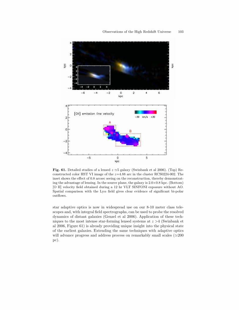
Observations of the High Redshift Universe 103
Fig. 61. Detailed studies of a lensed z ≃5 galaxy (Swinbank et al 2006). (Top) Re-constructed color HST VI image of the z=4.88 arc in the cluster RCS0224-002. Theinset shows the effect of 0.8 arcsec seeing on the reconstruction, thereby demonstrat-ing the advantage of lensing. In the source plane, the galaxy is 2.0×0.8 kpc. (Bottom)[O II] velocity field obtained during a 12 hr VLT SINFONI exposure without AO.Spatial comparison with the Lyα field gives clear evidence of significant bi-polaroutflows.
star adaptive optics is now in widespread use on our 8-10 meter class tele-scopes and, with integral field spectrographs, can be used to probe the resolveddynamics of distant galaxies (Genzel et al 2006). Application of these tech-niques to the most intense star-forming lensed systems at z >4 (Swinbank etal 2006, Figure 61) is already providing unique insight into the physical stateof the earliest galaxies. Extending the same techniques with adaptive opticswill advance progress and address process on remarkably small scales (≃200pc).

104 Richard S Ellis
A number of special purpose ground-based instruments are also being de-veloped, both with and without adaptive optics, to probe for z >7 dropoutsand Lyman α emitters. These include:
• The Dark Age Z Lyman Explorer (DAZLE, Horton et al 2004)9, a mod-erate field (7 arcmin) infrared narrow-band imager with airglow discrim-ination whose goal is to reach a sensitivity of ≃ 10−18 cgs in a night ofVLT time. This corresponds to a limiting star formation rate of ≃ 1M⊙
yr−1 in quiet regions of the airglow spectrum at z ≃7.7 and 9.9. Given themodest field and the need for dedicated spectroscopic follow-up, a longterm campaign is envisaged to conduct a reliable census.
• The Gemini Genesis Survey (GGS 10) which uses F2T2, a clone of thetunable filter destined for JWST (Scott et al 2006). This instrument isplanned to work behind the Gemini Observatory’s multi-conjugate adap-tive optics facility and image, in steps of wavelength, regions lensed byforeground clusters. The success of such a strategy will depend on boththe angular size and line widths of z >7 Lyman α emitters and the abun-dance of intrinsically faint examples. Ellis et al (2001) found the lensedemitter at z ≃5.7 was less than 30 milli-arcsec across with a line widthof only 100-200 kms sec−1. If such tiny emitters are the norm at z >7,the GGS may go much deeper than extant spectroscopic lensed searches(Stark et al 2006b).
The exciting redshift range 7< z < 12 will also be the province of improveddrop-out searches using the instrument WFC3 slated to be installed on HubbleSpace Telescope in 2008-911. The infrared channel of this instrument spans850 - 1170 nm with a field of ≃ 2 arcmin at an angular resolution of 0.13arcsec pixel−1. This resolution is coarser than that of adaptive optics-assistedinstruments such as F2T2. The principal gain over ground-based instrumentswill be in deep broad-band imaging free from airglow. The survey efficiencyis about an order of magnitude better than that of NICMOS. WFC3 also hastwo infrared grisms which will be helpful in source discrimination.
A major stumbling block at the moment, even at z ≃5-6, is efficient spec-troscopic follow-up of dropout candidates. As we discussed in §6, photometricredshifts have unfortunately become de rigeur in statistical analyses of lu-minosity densities and luminosity functions (Bouwens et al 2006), yet theirprecision remains controversial. For z- and J-band dropous beyond z ≃7, pho-tometric redshifts will be even less reliable. Spitzer detections will be harderand fewer, and the typical source may have only 2-3 detected bands. Candi-dates may be found in abundance but how will they be confirmed?
9 http://www.ast.cam.ac.uk∼optics/dazle/10 http://odysseus.astro.utoronto.ca/ggs-blog/?page id=211 http://www.stsci.edu/hst/wfc3

Observations of the High Redshift Universe 105
The various 8-10m telescopes are now building a new generation of cryo-genic near-infrared multi-slit spectrographs. It can be hoped that long expo-sures with these new instruments will be sufficient to break this impasse.
9.3 Beyond Five Years
A number of facilities are being planned, motivated by the progress discussedin these lectures. These include:
Fig. 62. The 6.5m James Webb Space Telescope: Then (2013 in orbit) and andNow (2005, full scale model).
• James Webb Space Telescope - a 6.5 meter optical-infrared space observa-tory (Gardner et al 2006) for which a primary mission is the detailed studyof the earliest star-forming galaxies (Figure 62). The facility is currently

106 Richard S Ellis
Fig. 63. The proposed US-Canadian Thirty Meter Telescope (www.tmt.org) nowin the detailed design phase.
planned to have a near-infrared imager NIRCam, a spectrograph NIRSpecwith both integral field and limited multi-object modes, a tunable filter (asF2T2) and a mid-IR imager, MIRI. Stiavelli (2002) has presented a cogentsummary of the likely strategies of using this facility, due to be launchedin 2013, for studies of the earliest systems.
• Extremely Large Telescopes on the ground including the US-CanadianThirty Meter Telescope (TMT, see www.tmt.org, Figure 63) which willhave a diffraction-limited near-infrared imager/spectrograph (IRIS) and aadaptive-optics assisted spectrograph (IRMOS) with multiple deployableintegral field units - area mapping units which can be arranged not onlyto scan regions surrounding luminous sources but also to undertake multi-object studies in crowded regions (Figure 64). At the time of writing, TMTis expected to be operational from 2016 onwards.
These will complement redshifted 21cm line tomography with radio fa-cilities and address the key questions of the escape fraction of photons fromstar-forming sources and how they create ionized bubbles which merge tocause reionization.
It is quite likely that, by 2013, the redshift range containing the earliestgalactic sources, estimated at present to be 10< z <20 perhaps, will have beenrefined sufficiently by special-purpose instruments on our existing 8-10 meterclass telescopes. Thus one can surmise that that both JWST and future ELTswill be used for much more challenging work related to the physical processof reionization, as well as the chemical maturity of the most luminous sourcesfound at high redshift.

Observations of the High Redshift Universe 107
Fig. 64. Flexibility in the deployment strategy for the multiple integral field units(yellow squares) for the proposed TMT infrared multi-object adaptive optics assistedinstrument IRMOS. The IFUs can be distributed around the full field of 2 arcminin classic multi-object mode. Alternatively, the IFUs can be configured together tomap a small 6 × 6 arcsec field at high angular resolution in ‘blind’ mode. Suchflexibility will be important in mapping Lyα emission at high redshift in varioussituations.
An obvious partnership between JWST and TMT, for example, whichwould complement the 21cm studies, would be to (i) search for the extent andtopology of faint Lyα emission in ionized bubbles around JWST-selected lu-minous star forming galaxies and, (ii) pinpoint early sources for spectroscopicscrutiny so as to identify signatures of Population III stars.
At the present time there are so many imponderables in our knowledge ofthe earliest sources, that even the design parameters for the ELT instrumentsis a considerable challenge. How big are the faintest Lyα emitters? What arethe typical line widths in km sec−1? How big are the ionized bubbles at agiven redshift? And, crucially, what is the surface density of various typesof star-forming galaxies. Flexibility in the design of survey strategies will becrucial with instruments such as TMT’s IRMOS (Fig. 64).
Any information we can glean on the properties of z ≃10 sources in thenext 5 years will be valuable in optimizing how to move forward when thesemagnificent new generation telescopes are made available to us. Indeed, it isfoolhardy to wait! Time and again, we can retrospectively look back at what

108 Richard S Ellis
we thought we would accomplish with our planned facilities and we alwaysfind that we achieved more than we expected!
10 Acknowledgements
I thank Daniel Schaerer, Denis Puy and Angela Hempel for inviting me togive these lectures in such a magnificent location with an enthusiastic groupof students. I also thank my fellow lecturers, Avi Loeb and Andrea Ferraraand all of the foregoing for their patience in waiting for the completion ofmy written lectures. I thank my close colleagues Kevin Bundy, Sean Moran,Mike Santos and Dan Stark for their help and permission to show resultsin progress as well as Ivan Baldry, Jarle Brinchmann, Andrew Hopkins, JohnHuchra and Jean-Paul Kneib for valuable input. Finally, I thank Ray Carlbergand his colleagues for their hospitality of the Astronomy Department at theUniversity of Toronto where the bulk of these lectures notes were completed.
Observations of the High Redshift Universe 109
11 References
Aaronson, M 1978 Ap J 221, L103Aharonian, F. et al 2006 Nature 440, 1018Adelberger, K et al 1998 Ap J 505, 18Astier, P. et al 2006 Astron. Astrophys., 447, 31Bahcall, N. et al 1999 Science 284, 1481Baldry, I. & Glazebrook, K. 2003 Ap J 593, 258Barkana, R. & Loeb, A 2000 Phys Rep. 349, 125Baugh, C. et al 1996 MNRAS 283, 1361Baugh, C. et al 1998 Ap J 498, 504Baugh, C. et al 2005a MNRAS 305, L21Baugh, C. et al 2005b MNRAS 356, 1191Becker, G et al 2006 Ap J in press, (astro-ph/0607633)Becker, R.H. et al 2001 AJ 122, 2850Beckwith, S. et al 2006 AJ 132, 1179Bell, E. et al 2004 Ap J 608, 752Bell, E. et al 2006 Ap J 640, 241Bender, R. et al 1992 Ap J 399, 462Bennett, C. et al 2003 Ap J Suppl., 148, 97Benson, A. et al 2002 MNRAS 336, 564Benson, A. et al 2003 Ap J 599, 38de Bernadis, P. et al 2000 Nature 404, 955Bernstein, R. et al 2002 Ap J 571, 56Blain, A. et al 2002 Phys. Rep. 369, 111Blain, A. et al 2004 Ap J 611, 725Blandford, R. & Narayan, R. 1992 ARAA 30, 311Blanton, M.R. et al 2001 A.J. 121, 2358Blumenthal, G. et al 1984 Nature 311, 517Bolton, A. et al 2006 Ap J 638, 703Bouwens, R. et al 2004 Ap J 606, L25Bouwens, R. et al 2006 Ap J in press (astro-ph/0509641)Bower, R. et al 1992 MNRAS 254, 601Bower, R. et al 2006 MNRAS 370, 645Brinchmann, J. & Ellis, R.S. 2000 Ap J 536, L77Broadhurst, T. et al 1992 Nature 355, 55Broadhurst, T. et al 2005 Ap J 621, 53Bruzual, G. 1980 Ph.D. thesis, UC BerkeleyBundy, K. et al 2004 Ap J 601, L123Bundy, K. et al 2005 Ap J 625, 621Bundy, K et al 2006 Ap J 651, 120Bunker, A. et al 2004 MNRAS 355, 374Bunker, A. et al 2006 New AR 50, 94Calzetti, D. et al 2000 Ap J 533, 682Caroll, S. et al 1992 ARAA 30, 499

110 Richard S Ellis
Chabrier, G. 2003 PASP 115, 763Chapman, S. et al 2003 Nature, 422, 695Chapman, S. et al 2005 Ap J 622, 772Conselice, C. et al 2005 Ap J 628, 160Cowie, L. et al 1995 AJ 109, 1522Cowie, L. et al 1996 AJ 112, 839Cole, S. et al 2000 MNRAS 319, 168Cole, S. et al 2001 MNRAS 326, 255Cole, S. et al 2005 MNRAS 362, 505Colless, M. et al 2001 MNRAS 328, 1039Couch, W. et al 1998 Ap J 497, 188Croton, D. et al 2006 MNRAS 365, 11Daddi, E. et al 2004 Ap J 617, 746Davies, R. L. et al 2001 Ap J 584, L33de Lucia, G. et al 2006 MNRAS 366, 499Dickinson, M. et al 2003 Ap J 587, 25Dickinson, M. et al 2004 Ap J 600, L99Djorgovski, S. & Davis, M. 1987 Ap J 313, 59Djorgovski, S. et al 2001 Ap J 560, L5Dole, H. et al 2006 Astron. Astrophys. 451, 417Dressler, A. 1980 Ap J 236, 351Dressler, A. et al 1987 Ap J 313, 42Dressler, A.. et al 1997 Ap J 490, 577Driver, S. et al 1995 Ap J 453, 48Drory, N. et al 2005 Ap J 619, L131Dube, R.R. et al 1979 Ap J 232, 333Dunlop, J. et al 2006 MNRAS in press (astro-ph/0606192)Ebbels, T. et al 1998 MNRAS 295, 75Eddington, A.S. 1919 Obs. 42, 119Egami, E. et al 2005 Ap J 618, L5Erb, D. et al 2006 Ap J 644, 813Ellis, R.S. 1997 ARAA 35, 389Ellis, R.S. et al 1996 MNRAS 280, 235Ellis, R.S. et al 2001 Ap J 560, L119Ellison, S. et al 2000 AJ 120, 1175Eyles, L. et al 2005 MNRAS 364, 443Eyles, L. et al 2006 MNRAS, in press (astro-ph/0607306)Fall, S. & Efstathiou, G. 1980 MNRAS 193, 189Fall, S. et al 1996 Ap J 464, L43Fan, X. et al 2003 AJ 125, 1649Fan, X. et al 2006a ARAA 44, 415Fan, X. et al 2006b AJ 132, 117Felton, J. E. 1977, AJ 82, 861Finkbeiner, D et al 2000 Ap J 544, 81Fontana, A. et al 2004 Astron. Astrophys., 424, 23.

Observations of the High Redshift Universe 111
Franx, M. et al 2003 Ap J 587, L79Frayer, D. et al 2000 AJ 120, 1668Freedman, W. et al 2001 Ap J 553, 47Fukugita, M. & Kawasaki, M. 2003 MNRAS 343, L25Fukugita, M. & Peebles, P.J.E. 2004 Ap J 616, 643Fukugita, M. et al 1998 Ap J 503, 518Furlanetto, S. et al 2005 Phys. Reports 433, 181Gardner, J. et al 2006 Space Sci. Rev. in press (astro-ph/0606175)Genzel, R. et al 2006 Nature 442, 786Gerhard, O. et al 2001 AJ 121, 1936Giavalisco, M. et al 2004 Ap J 600, 103Glazebrook, K. et al 1995 MNRAS 275, L19Glazebrook, K. et al 2004 Nature 430, 181Gradshteyn, I.S. & Ryzhik, I.M. 2000, Tables of Integrals, Series and Products,Academic PressGranato, G.L. et al 2000 Ap J 542, 710Gunn, J.E. & Peterson, B.A. 1965 Ap J 142, 1633Haiman, Z. 2002 Ap J 576, 1Hanany, et al 2000 Ap J 545, 5Hauser, M & Dwek, E 2001 ARAA 39, 249Hauser, M. et al 1998 Ap J 508, 25Hoekstra, H. et al 2005 Ap J 647, 116Hopkins, A.M. 2004 Ap J 615, 209Hopkins, A.M. & Beacom, J. 2006 Ap J 651, 142Horgan, J. 1998 The End of Science, Addison-WesleyHorton, A. et al 2004 in Ground-based Instrumentation for Astronomy, S.P.I.E.5492, 1022Hu, E. et al 2004 AJ 127, 563Hubble, E. 1936 The Realm of the Nebulae, Yale Univ. PressHughes, D. et al 1998 Nature 394, 241Iye, M. et al 2006 Nature 443, 186Jorgensen, I. et al 1996 MNRAS 280, 167Jullo, E et al 2006, Astron. Astrophys, submittedJuneau, S. et al 2005 Ap J 619, L135Kaiser, N. et al 1987 MNRAS 277, 1Kauffmann, G. & Charlot, S. 1998 MNRAS 297, L23Kauffmann, G. et al 1993 MNRAS 264, 201Kauffmann, G. et al 1996 MNRAS 283, L117Kauffmann, G. et al 1999 MNRAS 303, 188Kauffmann, G. et al 2003 MNRAS 341, 33Kashikawa, N. et al 2006 Ap J 648, 7Kashlinsky 2005 Phys. Reports 409, 361Kashlinsky et al 2002 Ap J 579, 53Kashlinsky et al 2005 Nature 438, 45Kashlinsky et al 2006 Ap J Lett in press (astro-ph/0612445)

112 Richard S Ellis
Kelsall, T. et al 1998 Ap J 508, 44Kennicutt, R. 1983 Ap J 272, 54Kennicutt, R. 1998 ARAA 36, 189Kneib, J-P. et al 1996 Ap J 471, 643Kneib, J-P. et al 2004 Ap J 607, 697Kodaira, I. et al 2003 PASJ 55, L17Kogut, A. et al 2003 Ap J Suppl., 148, 161.Kong et al 2006 Ap J 638, 72Koo, D. & Kron, R. 1992 ARAA 30, 613.Koopmans, L. & Treu, T. 2003 Ap J 583, 606Kriek, M. et al 2006 Ap J 649, L71Kroupa, P. et al 1993 MNRAS 262, 545Kroupa, P. 2001 MNRAS 332, 231Lanzetta, K. et al 2002 Ap J 570, L492Leinert, C. et al 1995 Astron. Astrophys. Suppl. 112, 99Le Fevre, O. et al 2000 MNRAS 311, 565Lilly, S.J. et al 1996 Ap J 460, L1McCarthy, P. 2004 ARAA 42, 477McCarthy, P. et al 2004 Ap J 614, L9McClure, R. et al 2006 MNRAS 372, 357Madau, P. & Pozzetti, L. 2000 MNRAS 312, L9Madau, P. & Silk, J. 2005 MNRAS 359, L37Madau, P. et al 1996 MNRAS 283, 1388Madau, P. et al 1998 Ap J 498, 106Madau, P. et al 1999 Ap J 514, 648Maddox, S. et al 1990 MNRAS 242, 43Malhotra, S. & Rhoads, J. 2004Malhotra, S. et al 2005 Ap J 627, 666Malin, D. & Carter, D 1980 Nature 285, 643Mather, J. et al 1990 Ap J 354, 37Mattilia, K. 1976 Astron. Astrophys. 47, 77Mattila, K. 2003 Ap J 591, 119Mattila, K. 2006 MNRAS 372, 1253Matsumoto, T. et al 2005 Ap J 626, 31Meier, D.L. 1976 Ap J 207, 343Mellier, Y. 2000 ARAA 37, 127Miller, G.E. & Scalo, J. 1979 Ap J Suppl. 41, 513Miralda-Escude, J. et al 1998 Ap J 501, 15Mobasher, B. et al 2005 Ap J 635, 832Nagamine, et al 2004 Ap J 610, 45Nagao, T. et al 2005 Ap J 634, 142Newman J. & Davis, M 2000 Ap J 534, L11Norberg, P et al 2002 MNRAS 336, 907Oppenheimer, B.D. et al 2006 in Chemodynamics: First Stars to Local Galax-
ies, in press (astro-ph/0610808)

Observations of the High Redshift Universe 113
Ostriker, J. & Peebles, P. 1973 Ap J 186, 467Ostriker, J & Steinhardt, P. 1996 Nature 377, 600Ouchi, M. et al 2005 Ap J 620, L1Papovich, C. et al 2006 Ap J 640, 92Partridge, B. & Peebles, P.J.E. 1967 Ap J 147, 868Peacock et al 2001 Nature 410, 169Peebles, P. 1980 Large Scale Structure of the Universe, Univ. Chicago.Penzias, A. & Wilson, 1965 Ap J 142, 419Perlmutter, S. et al 1999 Ap J 517, 565Pettini, M. et al 2002 Astrophys. Sp. Sci. 281, 461Postman, M. et al 2005 Ap J 623, 721Pritchet, C. 1994 PASP 106, 1052Reddy, N. et al 2005 Ap J 633, 748Refregier, A. 2003 ARAA 41, 645Richard, J. et al 2006 Astron. Astrophys. 456, 861Riess, A. et al 1995 AJ 116, 1009Rowan-Robinson, M. 1985 The Cosmic Distance Scale (Freeman)Rubin, V. 2000 PASP 112, 747Rubin, V. et al. 1976 AJ 81, 687Rudnick, G. et al 2003 Ap J 599, 847Salpeter, E. 1955 Ap J 121, 161Sand, D.J. et al 2005 Ap J 627, 32Sandage, A. 2005 ARAA 43, 581Santos, M. 2004 MNRAS 349, 1137Santos, M. et al 2004 Ap J 606, 683Sargent, M.T. et al Ap J in press (astro-ph/0609042)Seitz, et al 1998 MNRAS 298, 945Scalo, J. 1986 Fund. Cosmic Phys. 11, 1Schechter, P. 1976 Ap J 203, 297Schlegel, D. et al 1998 Ap J 500, 525Schneider, P. 2006 in Gravitational Lensing: Strong, Weak & Micro, Saas-FeeAdvanced Course 33Scott, A. et al 2006 in Ground-based and Airborne Instrumentation for As-
tronomy, S.P.I.E. 6269, 176Shapley, A. et al 2001 Ap J 562, 95Shapley, A. et al 2003 Ap J 588, 65Shapley, A. et al 2005 Ap J 626, 698Shimasaku, K. et al 2005 PASJ 57, 447Shioya Y. et al 2005 PASJ 57, 287Smail, I. et al 1995 Ap J 440, 501Smail, I. et al 1997 Ap J 490, L5Smith, G. et al 2005 Ap J 620, 78Smoot, G. et al 1992 Ap J 396, 1Somerville, R. & Primack, J. 1999 MNRAS 310, 1087Somerville, R. et al 2001 MNRAS 320, 504

114 Richard S Ellis
Somerville, R. et al 2004 Ap J 600, L171Songaila, A. 2004 AJ 127, 2598Songaila, A. 2005 AJ 130, 1996Songaila, A. 2006 AJ 131, 24Spergel, D. et al 2003 Ap J Suppl. 148, 175Spergel, D. et al 2006 Ap J in press (astro-ph/0603449)Springel, V. et al; 2005 Nature 435, 629Stanway, E. et al 2004 Ap J 607, 704.Stanway, E. et al 2005 MNRAS 359, 1184Stark, D. & Ellis, R.S. 2005 New AR 50, 46Stark, D. et at 2006a Ap J in press (astro-ph/0604250)Stark, D. et al 2006b Ap J submittedStiavelli, M. 2002 in Future Research Directions & Visions for Astronomy,S.P.I.E. 4835, 122Stiavelli, M. et al 2004 Ap J 600, 508Steidel, C. et al 1996 Ap J 492, 428Steidel, C. et al 1999a Ap J 519, 1Steidel, C. et al 1999b Phil Trans R. Soc. 357, 153Steidel, C. et al 2003 Ap J 592, 728Struck-Marcell, & Tinsley, B. 1978 Ap J 221, 562Sullivan, I. et al 2006 Ap J in press (astro-ph/0609451)Sullivan, M. et al 2000 MNRAS 312, 442Sullivan, M. et al 2001 Ap J 558, 72Swinbank, M. et al 2006 Ap J submittedTaniguchi, Y. et al 2005 PASJ 57, 165Tinsley, B. 1980 Fund. Cosmic Phys. 5, 287Toomre, A. & Toomre, J 1972 Ap J 178, 623Tran, K.-V. et al 2005 Ap J 627, L25Treu, T. et al 2005 Ap J 622, L5Treu, T et al 2006 Ap J 640, 662Tully, B. & Fisher, 1977 Astron. Astrophys. 54, 661van der Wel, A. et al 2005 Ap J 631, 145van der Wel, A. et al 2006 Ap J 636, L21van Dokkum, P. 2005 AJ 130, 2647van Dokkum, P. & Ellis, R.S. 2003 Ap J 592, L53van Dokkum, P. et al 2003 Ap J 587, L83van Dokkum, P. et al 2006 Ap J 638, L59Vogt, N. et al 1996 Ap J 465, L15Vogt, N. et al 1997 Ap J 479, L121Weiner, B. et al 2005 Ap J 620, 595Wright, E. & Reese, E.D. 2000 Ap J 545, 43Yan, H. & Windhorst, R. 2004 Ap J 612, 93Yan, H. et al 2005 Ap J 634, 109Yan, H. et al 2006 Ap J 651, 24Yee, H. et al 1996 AJ 111, 1783

Observations of the High Redshift Universe 115
York, D. et al 2001 AJ 120, 1579Zwaan, M.A. et al 2003 AJ 125, 2842Zwicky, F. 1933 Helv. Physica Acta, 6, 110Zwicky, F. 1937 Phys Rev. 51, 290