observations of the small-scale variability of …boonleng/pdf/palmer++05.pdfobservations of the...

Observations of the Small-Scale Variability of Precipitation Using an Imaging Radar

ROBERT D. PALMER

School of Meteorology, University of Oklahoma, Norman, Oklahoma

BOON LENG CHEONG AND MICHAEL W. HOFFMAN

Department of Electrical Engineering, University of Nebraska at Lincoln, Lincoln, Nebraska

STEPHEN J. FRASIER AND F. J. LÓPEZ-DEKKER

Department of Electrical and Computer Engineering, University of Massachusetts—Amherst, Amherst, Massachusetts

(Manuscript received 16 September 2004, in final form 11 February 2005)

ABSTRACT

For many years, spatial and temporal inhomogeneities in precipitation fields have been studied usingscanning radars, cloud radars, and disdrometers, for example. Each measurement technique has its ownadvantages and disadvantages. Conventional profiling radars point vertically and collect data while theatmosphere advects across the field of view. Invoking Taylor’s frozen turbulence hypothesis, it is possibleto construct time-history data, which are used to study the structure and dynamics of the atmosphere. In thepresent work, coherent radar imaging is used to estimate the true three-dimensional structure of theatmosphere within the field of view of the radar. The 915-MHz turbulent eddy profiler radar is well suitedfor imaging studies and was used in June 2003 to investigate the effects of turbulence on the formation ofrain. The Capon adaptive algorithm was implemented for imaging and clutter rejection purposes. In the pastseveral years, work by the authors and others has proven the Capon method to be effective in this regardand to possess minimal computational burden. A simple but robust filtering procedure is presented wherebyechoes from precipitation and clear-air turbulence can be separated, facilitating the study of their interac-tion. By exploiting the three-dimensional views provided by this imaging radar, it is shown that boundarylayer turbulence can have either a constructive or destructive effect on the formation of precipitation.Evidence is also provided that shows that this effect can be enhanced by updrafts in the wind field.

1. Introduction

Modern atmospheric radars are typically operated inthe VHF band for observations of the structure anddynamics of clear-air turbulence from the troposphereto the mesosphere (Woodman and Guillen 1974).These radars often have large apertures (50–100 m)with corresponding beamwidths of 3°–6°. Also knownas mesosphere–stratosphere–troposphere (MST) radar,such research systems have been used successfully fordecades for measurements of wind and reflectivityfields. Systems operating close to 400 MHz have beendesigned for operational use and are deployed across

the central region of North America (Weber et al.1990). For studies of the atmospheric boundary layer(ABL), shorter-wavelength radars, of a similar design,are used and are commercially available. These bound-ary layer radars (BLRs) operate near 1 GHz and arecapable of observations from near 100 m to a few kilo-meters in altitude, depending on the atmospheric con-ditions (Ecklund et al. 1988).

Originally developed for observations of the iono-sphere (Pfister 1971; Woodman 1971), spatial interfer-ometry (SI) has proven to be very useful for high-resolution localization of coherent structures (e.g., Far-ley et al. 1981; Kudeki et al. 1981; Röttger and Ierkic1985). Spatial interferometry is based on the use ofinterference patterns in coherent signals received fromspatially separated antennas. Many factors can affectthe interference pattern, including the wind field andthe structure of the scatterers. It has also been shown

Corresponding author address: Robert D. Palmer, Dept. of Me-teorology, University of Oklahoma, 100 E. Boyd, Room 1310,Norman, OK 73019.E-mail: [email protected]

1122 J O U R N A L O F A T M O S P H E R I C A N D O C E A N I C T E C H N O L O G Y VOLUME 22

© 2005 American Meteorological Society

JTECH1775

that the size distribution of precipitation particles canaffect the SI method (Chilson et al. 1995). Of course, itis just these effects that are used to study the physics ofthe atmosphere.

By coherently summing signals from an interferomet-ric radar system, rudimentary beam forming (imaging)is possible. These simple methods, based on the spatialFourier transform, were termed postset beam steering(Röttger and Ierkic 1985) and poststatistic steering(Kudeki and Woodman 1990; Palmer et al. 1993). Thefirst true imaging experiments using several spatiallyseparated receive elements were conducted by Kudekiand Sürücü (1991) for observations of the equatorialelectrojet. The term coherent radar imaging (CRI) wascoined for this beam-forming process. The maximumentropy method was later employed to enhance angularresolution (Hysell 1996). Subsequently, Palmer et al.(1998) used the data-dependent algorithm based on thework of Capon (1969) for observations of clear-air tur-bulence and precipitation using the Middle and Upper(MU) Atmosphere radar. More recently, this methodhas been used to study the dynamics of coherent echoesfrom the polar mesosphere (Yu et al. 2001). Given thenumerous algorithms available for CRI applications,statistical investigations have been undertaken to de-termine the advantages and disadvantages of each tech-nique (e.g., Yu et al. 2000; Chau and Woodman 2001).An attempt to generalize the theory of radar imaginghas been made by Woodman (1997). For a review of therelevant literature, see Luce et al. (2001).

Given the increasing need for higher-resolution mea-surements, new or upgraded systems have been devel-oped to exploit the potential of imaging. For example,a French radar has been recently modified to allow theimplementation of imaging methods (Hélal et al. 2001).The MU radar, which has been used successfully formany years (Fukao et al. 1985a,b), has also undergonea significant upgrade to 25 independent receivers. Forapplications to tropical meteorology, plans are also un-derway that would facilitate the implementation of im-aging on the Indian MST radar (Rao et al. 1995; Jain etal. 1995). As mentioned earlier, radar observations ofthe ABL are typically conducted using frequenciesclose to 1 GHz. With the goal of real-time mapping thethree-dimensional turbulent field of the ABL, the tur-bulent eddy profiler (TEP) was developed by research-ers at the University of Massachusetts (Mead et al.1998). This 915-MHz BLR has up to 64 independentreceivers, allowing the use of sophisticated imaging al-gorithms with unprecedented flexibility. The system iscapable of mapping a conical volume above the radarlimited by the beamwidth of the transmit antenna. TEPhas been used for observations of the convective

boundary layer (CBL), which compared favorably tonumerical simulations (Pollard et al. 2000). In conjunc-tion with a radio acoustic sounding system, the TEPradar was used to study the propagation and distortionof acoustic waves (Lopez-Dekker and Frasier 2004).The goal of the present work is to show the usefulnessof the TEP radar for small-scale studies of precipita-tion.

Precipitation is often characterized by the drop sizedistribution (DSD), which is in turn used to quantifyrainfall rate, for example. Using scanning weather ra-dar, studies have been conducted to investigate the spa-tial and temporal variability of rainfall rate (Crane1990). However, the spatial resolution was on the orderof kilometers. In a series of papers, Jameson et al.(1999, and references therein) have brought into ques-tion assumptions concerning the homogeneity of pre-cipitation. Recently, observations of convective precipi-tation have shown the Doppler sorting effect caused byupdrafts (Kollias et al. 2001). In addition, the interac-tion of cloud particles and turbulence has been re-viewed by Vaillancourt and Yau (2000). Previous workusing a 915-MHz BLR has shown the effect that lightrain can have on the reflectivity of turbulent layers(Cohn et al. 1995). Here, we present data from the TEPradar that show the significant influence of turbulenceon the formation of precipitation. It is further shownthat the mean vertical wind can enhance this effect.Three-dimensional images of precipitation and clear-airturbulence echoes are provided, exemplifying the inter-play of these distinct atmospheric phenomena.

In the next section, the experimental configurationusing TEP is presented. Then, the meteorological con-ditions during the experiment are analyzed. Finally, re-sults from both standard processing and imaging aregiven in an attempt to understand the effects of ABLturbulence on the precipitation that occurred duringthe experiment.

2. Experimental configuration using the turbulenteddy profiler

An extensive experiment was conducted in Amherst,Massachusetts, in June 2003 using the TEP radar withthe goal of assessing the capabilities of the system forobserving a variety of boundary layer phenomena. Justprior to the observations, a cold front had pushed offthe southeastern coast of the United States with a weaklow pressure system off the Massachusetts coast. Anupper-level low was located just south of the surfacelow, resulting in counterclockwise winds flowingaround the cyclone. This wind, along with the cold airmass present to the southwest of Massachusetts, caused

AUGUST 2005 P A L M E R E T A L . 1123

overrunning of warm air and sporadic light rain duringthe experiment.

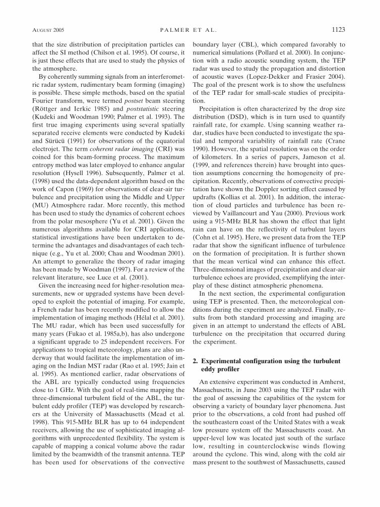
In its current configuration, the 915-MHz TEP radarconsists of a transmit horn antenna and a receive arrayof up to 64 microstrip patch elements separated by ap-proximately 0.57 m (Mead et al. 1998; Lopez-Dekkerand Frasier 2004). The exact number of elements isdependent upon the array configuration used. Signalsfrom each receive element are sent through a low-noiseamplifier before being fed to the control trailer. Thesesignals are input to individual analog receivers and co-herently integrated on specially designed integrated-circuit boards, each with four receivers. The coherentlyintegrated in-phase and quadrature signals are thenstored to disk for further processing. By coherentlycombining the signals from the individual elements, it ispossible to image the atmosphere in a cone-shaped vol-ume above the radar. A depiction of the TEP imagingconcept is provided in Fig. 1. The transmit beamwidthof TEP is shown as the relatively wide angular regionthat defines the field of view of the radar. Imaging con-sists of combining the individual receiver signals in or-der to synthesize narrow focused beams within thetransmit beam. By adjusting the method by which thesignals are combined, it is possible to create a map, orimage, of the atmosphere above the radar. This processis conducted for each range gate individually, resultingin a three-dimensional image. Given the inherent flex-ibility designed into the TEP array, it is also possible toinvestigate advantages of various array configurationsand processing schemes. Data from one of these con-figurations are discussed here in the context of the spa-tial variability of precipitation on scales less than theoverall size of the TEP volume, which has a maximumhorizontal dimension of approximately 1 km.

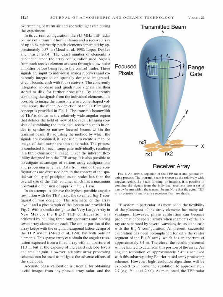
In an attempt to achieve the highest possible angularresolution with the TEP array, the so-called Big-Y con-figuration was designed. The schematic of the arraylayout and a photograph of the system are provided inFig. 2. With a similar design to the Very Large Array inNew Mexico, the Big-Y TEP configuration wasachieved by building three outrigger arms and placingseven array elements on each. The center portion of thearray keeps with the original hexagonal lattice design ofthe TEP system (Mead et al. 1998) but with only 37elements. This sparse array can obtain the angular reso-lution expected from a filled array with an aperture of11.3 m but at the expense of increased sidelobe levelsand smaller gain. However, adaptive array processingschemes can be used to mitigate the adverse effects ofthe sidelobes.

Accurate phase calibration is essential for obtaininguseful images from any phased array radar, and the

TEP system in particular. As mentioned, the flexibilityof the placement of the array elements has many ad-vantages. However, phase calibration can becomeproblematic for sparse arrays when segments of the ar-ray are separated by several wavelengths, as is the casewith the Big-Y configuration. At present, successfulcalibration has been accomplished for only the centersegment of the Big-Y array, which has an aperture ofapproximately 3.4 m. Therefore, the results presentedwill be limited to data from this portion of the array. Anangular resolution of approximately 5.4° is achievedwith this subarray using Fourier-based array processingschemes. However, high-resolution algorithms will beexploited to improve the resolution to approximately2.7 (e.g., Yu et al. 2000). As mentioned, the TEP radar

FIG. 1. An artist’s depiction of the TEP radar and general im-aging process. The transmit beam is shown as the relatively wideangular region. By beam forming, or imaging, it is possible tocombine the signals from the individual receivers into a set ofnarrow beams within the transmit beam. Note that the actual TEParray consists of many more receivers than are shown.


Fig 1 live 4/C

was originally designed to incorporate a separate trans-mit antenna, which can be seen in the background ofthe photograph of Fig. 2. As a result, no high-speed T/Rswitch was necessary, and observations close to the sur-face were facilitated. The current transmit horn an-tenna has a 25° one-way, half-power, beamwidth thatdefines the imaged volume. At an altitude of 2 km, thevolume has a coverage width of approximately 887 m.The peak transmit power was 4 kW.

The pulse repetition frequency (PRF) was set to 35kHz with 250 coherent integrations, resulting in an ef-fective sampling time of 7.14 ms. Given the operatingfrequency of 915 MHz, the aliasing velocity for the ex-periment was 11.48 m s�1, which was adequate for themaximum radial velocities expected in the boundarylayer. Data blocks consisting of 260 time series pointsfrom all receivers were recorded every 2.5 s, includingoverhead for storage and online processing. Most of theresults to be presented were obtained using two inco-herent integrations, resulting in an approximate 5-stemporal resolution. A pulse width of 222 ns was used,providing 33.3-m range resolution. At a nominal alti-tude of 1 km and given the expected angular resolutionof 2.7°, the TEP configuration used for the present ex-periment was capable of observations of approximately47 m � 47 m � 33 m subvolumes within the overallvolume defined by the transmit beam. Sixty-four (64)range gates were sampled from just before the transmitpulse was launched to a maximum time correspondingto an altitude of 1.93 km. Of course, the gates sampledbefore the transmit beam are not useful. Further,ground clutter limited the lowest observable altitude to

approximately 100 m using our adaptive clutter rejec-tion algorithms (Palmer et al. 1998).

With the given sampling rate and the numerous re-ceivers of the TEP radar, it was difficult to continuouslyrecord data for periods longer than several hours. Thedata presented here were taken on 21 June 2003, overthe 3-h period 1805–2105 UTC. Although transport-able, the TEP radar was used while deployed at theexperimental home facility operated by the Universityof Massachusetts, Amherst (42.38°N, 72.52°W).

3. Experimental results

Raw in-phase and quadrature data from this experi-ment were processed offline in order to generate three-dimensional images of echo power and radial velocitywithin the field of view of the radar (�12.5°). The com-plex time series data from each of the 37 receivers werecombined using previously developed imaging methodsbased on data-adaptive concepts (Palmer et al. 1998).Let the time-domain signals from the 37 receivers becombined into the data vector denoted by x(t). Theimaging process is accomplished by linearly combiningthe 37 signals by the following simple vector multipli-cation,

y�t� � w†x�t�, �1�

where the dagger represents the Hermitian operator(conjugate transpose). The scalar time-domain signaly(t) corresponds to the angular position within the fieldof view determined by the complex weighting vector w,which is a function of the desired zenith and azimuth

FIG. 2. (a) TEP receive array configuration along with a photograph from the experiment. Shading on the array schematic providesprecise measurements of the element heights, which are essential for phase calibration. The overall aperture of this sparse arrayapproaches 11.3 m. (b) The photograph shows the array with the transmit horn antenna in the background.


Fig 2 live 4/C

angles. By adjusting w to scan through the field of view,the resulting set of y(t) signals can be used to estimatemaps of Doppler spectra, or simply echo power andradial velocity, using standard algorithms (Cheong et al.2004). Of course, this process is typically carried out foreach range gate individually and therefore provides athree-dimensional view of the atmosphere above theradar.

To achieve high angular resolution and mitigate theeffects of both ground and biological clutter, the adap-tive Capon method (Capon 1969) was chosen for gen-eration of the weighting vector w. Many other algo-rithms have been developed for the imaging process(e.g., Haykin 1985; Kudeki and Sürücü 1991; Hysell1996) but the authors have found the Capon method toprovide good resolution with only moderate computa-tional complexity (Yu et al. 2000). For a complete deri-vation of the Capon weighting vector for the atmo-spheric imaging case, see Palmer et al. (1998). For thepresent study, it is sufficient to say that the complexweighting vector w is data dependent and is systemati-cally adjusted for each solid angle within the field ofview of the radar, as shown in Fig. 1.

a. Echo power and vertical motion

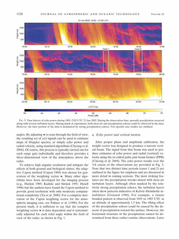
After proper phase and amplitude calibration, theweight vector was designed to produce a narrow verti-cal beam. The signal from that beam was used to pro-duce estimates of echo power and radial (vertical) ve-locity using the so-called pulse pair beam former (PPB)(Cheong et al. 2004). The echo power results over the3-h extent of the observations are provided in Fig. 3.Note that two distinct time periods (cases 1 and 2) areoutlined in the figure for emphasis and are discussed inmore detail in coming sections. The most striking fea-tures are the precipitation streaks mixed with clear-airturbulent layers. Although often masked by the rela-tively strong precipitation echoes, the turbulent layersoften show patterns indicative of Kelvin–Helmholtz in-stabilities (Gossard 1990). For example, a classicbraided pattern is observed from 1855 to 1905 UTC atan altitude of approximately 1.5 km. The tilting effectof the precipitation echoes could be caused by the de-scent of precipitation toward the surface. However, thehorizontal structure of the precipitation cannot be de-termined from these rather routine observations. Later

FIG. 3. Time history of echo power during 1805–2105 UTC 21 Jun 2003. During the observation time, sporadic precipitation occurredalong with several turbulent layers. During much of experiment, both clear-air and precipitation echoes could be observed in the data.However, the later portion of the data is dominated by strong precipitation echoes. Two specific case studies are outlined.


Fig 3 live 4/C

sections deal with horizontal structure through the useof imaging. For now, it is assumed that the echoes arecaused by sporadic precipitation. The fall speed can beestimated by the apparent tilt of the rain streaks in theecho power time-history plot. For example, the rainstreaks occurring at 1835 UTC descend from the top ofthe observation range (1.93 km) to the surface in ap-proximately 4 min, which corresponds to an 8 m s�1 fallvelocity. Assuming no vertical wind, a terminal fall ve-locity of this magnitude could result from drops withdiameters close to 3 mm (Gunn and Kinzler 1949).

Another interesting feature observed is the interac-tion between the turbulent layers and the precipitation.Work by Cohn et al. (1995) has shown that rain canaffect the reflectivity measured by radar. It is alsoknown that turbulent flow can have a significant effecton both the spatial and velocity distributions of clouddroplets (Vaillancourt and Yau 2000). Further, rain canexhibit clustering caused by small-scale turbulence dueto its effect on collisions and the resulting coalescenceor breakup (Pruppacher and Klett 1997; Jameson et al.1999). Contrasting examples of the interaction of rainwith turbulent layers can be observed at 1944 and 1955

UTC. At 1944 UTC, relatively weak precipitation isseen in the upper ranges. After passing through theturbulent layer at an altitude of approximately 800 m,the intensity of the echo increases significantly, indicat-ing significant coalescence. In contrast, the precipita-tion echo at 1955 UTC appears at the upper altitudesbut is then dissipated just below the turbulent layer atapproximately 1000 m. The exact cause could be re-lated to evaporation or breakup. Nevertheless, the cor-relation between the location of dissipation and the tur-bulent layer is unmistakable. Using imaging, the three-dimensional spatial structure of these events is studiedin more detail in later sections.

The time history of the vertical velocity is provided inFig. 4. The color scale was chosen so that negative(downward) velocities are shaded in blue, zero is white,and red tints are positive (upward). The mixture of thefalling precipitation and oscillating clear-air turbulencemakes the data difficult to interpret. Nevertheless, thetilted rain echoes are seen to have vertical velocitiesfrom �8 to �2 m s�1. The velocities corresponding toclear-air echoes are seen to oscillate with periods on theorder of minutes.

FIG. 4. Same as previous figure, except for vertical velocity. Note that the color scale is centered around large negative velocities toemphasize the precipitation.


Fig 4 live 4/C

The 33-cm wavelength of the TEP radar allows thesimultaneous observation of Bragg-scale turbulenceand precipitation, which causes Rayleigh scatter. Ofcourse, this can make interpretation rather problem-atic. In the next section, it is shown how frequencyselectivity can be used with imaging to separate thesedistinct echoes, facilitating their study.

b. Feature separation using frequency-selectiveimaging

Under certain conditions, Doppler spectra from ver-tically pointing radar can exhibit two peaks—one dueto clear-air turbulence and the other to precipitation(Wakasugi et al. 1986). A sequence of just such spectrais shown in Fig. 5 for 12 frames from 1851:01 to 1852:54UTC. In the first frame, a precipitation echo is ob-served at an altitude of approximately 1 km with an

apparent fall speed close to �8 m s�1. As time pro-gresses through the 12 frames, the layer is seen to falltoward the surface. During the entire event, obviousclear-air echoes are seen throughout the observationrange. These echoes can be discriminated from the pre-cipitation echoes by their relatively small vertical ve-locities. Typical clear-air vertical velocities in a noncon-vective environment will rarely exceed �2 m s�1.

Using a similar technique to Palmer et al. (1998), it ispossible to exploit the distinct vertical velocity charac-teristics of clear-air turbulence and precipitation toseparate the two processes. This is accomplished bypassing the individual receiver signals through temporalfilters before the imaging process. The precipitation sig-nal was extracted by passing the 37 receivers’ time se-ries signals through an eighth-order, high-pass, ellipticalfilter (HPF). A cutoff velocity of �2 m s�1 was chosen,virtually eliminating the clear-air echo. Output signals

FIG. 5. Time sequence of Doppler spectra for a 2-min period (1851:01–1852:54 UTC). A layer of precipitation can initially be seenat an altitude of approximately 1 km and progresses to the surface with time. Note the simultaneous clear-air echoes with radialvelocities less than �2 m s�1.


Fig 5 live 4/C

were then used for the imaging process in the samemanner as that used to produce Fig. 3. The synthesizedprecipitation echo power, free from clear-air contami-nation, is shown in Fig. 6. Due to the non-ideal HPFfilter, some residual clear-air signal is present in thedata. Nevertheless, many features not obvious beforefiltering are now prominent and are discussed in moredetail in the next section.

A significant advantage is realized when the comple-mentary filtering process is implemented by passing the37 time series signals through a low-pass filter (LPF) ofa design similar to that of the HPF. Again, the cutoffvelocity was set to �2 m s�1, but the filter was designedto attenuate the precipitation echo. However, by tem-porally filtering before imaging, the input-filtered signaloriginates from a wider angular region than would havebeen the case if imaging had been performed first. Atlarge off-vertical angles, the geometric projection (ra-dial velocity) of the fall speed of the precipitation maybe small enough to allow a precipitation signal to passthrough the filter. Although much more cumbersomeand computationally expensive, imaging before tempo-ral filtering would mitigate this possible artifact. Nev-

ertheless, given the �12.5° transmit beamwidth, thisfilter leakage effect should be small. The resulting syn-thesized clear-air echo power is provided in Fig. 7. Notehow the filtering/imaging process reveals coherentstructure in the time history that was completelymasked by precipitation in Fig. 3. In particular, thelower panel of the figure (2005–2105 UTC) shows abraided structure at an altitude of 100–500 m for 2005–2025 UTC. It would have been impossible to studythese echoes without the use of the LPF and imaging.

There are two well-known, radar-based methods ofestimating turbulent intensity. The first uses the radarreflectivity (�) of turbulence within the resolution vol-ume to estimate the structure function parameter ofrefractivity C2

n, which is a measure of turbulent inten-sity. Tatarskii (1961) showed the following formulation:

� � 0.38Cn2��1�3, �2�

where � is the radar wavelength. It is assumed thatturbulence exists and is isotropic and in the inertialsubrange. Further, the radar resolution volume is as-sumed to be uniformly filled with turbulence. Given the

FIG. 6. Time history of synthesized precipitation echo power. These data were obtained by high-pass filtering before the imagingprocess, which isolates the precipitation echo from the clear-air turbulent echo.


Fig 6 live 4/C

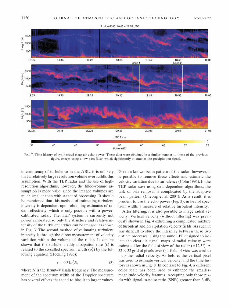
intermittency of turbulence in the ABL, it is unlikelythat a relatively large resolution volume ever fulfills thisassumption. With the TEP radar and the use of high-resolution algorithms, however, the filled-volume as-sumption is more valid, since the imaged volumes aremuch smaller than with standard processing. It shouldbe mentioned that this method of estimating turbulentintensity is dependent upon obtaining estimates of ra-dar reflectivity, which is only possible with a power-calibrated radar. The TEP system is currently notpower calibrated, so only the structure and relative in-tensity of the turbulent eddies can be imaged, as shownin Fig. 3. The second method of estimating turbulentintensity is through the direct measurement of velocityvariation within the volume of the radar. It can beshown that the turbulent eddy dissipation rate () isrelated to the so-called spectrum width (2

�) by the fol-lowing equation (Hocking 1986):

� � 0.31��2N, �3�

where N is the Brunt–Väisälä frequency. The measure-ment of the spectrum width of the Doppler spectrumhas several effects that tend to bias it to larger values.

Given a known beam pattern of the radar, however, itis possible to remove these effects and estimate thevelocity variation due to turbulence (Cohn 1995). In theTEP radar case using data-dependent algorithms, thetask of bias removal is complicated by the adaptivebeam pattern (Cheong et al. 2004). As a result, it isprudent to use the echo power (Fig. 3), in lieu of spec-trum width, a measure of relative turbulent intensity.

After filtering, it is also possible to image radial ve-locity. Vertical velocity (without filtering) was previ-ously shown in Fig. 4 exhibiting a complicated mixtureof turbulent and precipitation velocity fields. As such, itwas difficult to study the interplay between these twodistinct processes. Using the same LPF designed to iso-late the clear-air signal, maps of radial velocity wereestimated for the field of view of the radar (�12.5°). A32 � 32 grid of pixels over this field of view was used tomap the radial velocity. As before, the vertical pixelwas used to estimate vertical velocity, and the time his-tory is shown in Fig. 8. In contrast to Fig. 4, a differentcolor scale has been used to enhance the smaller-magnitude velocity features. Accepting only those pix-els with signal-to-noise ratio (SNR) greater than 3 dB,

FIG. 7. Time history of synthesized clear-air echo power. These data were obtained in a similar manner to those of the previousfigure, except using a low-pass filter, which significantly attenuates the precipitation signal.


Fig 7 live 4/C

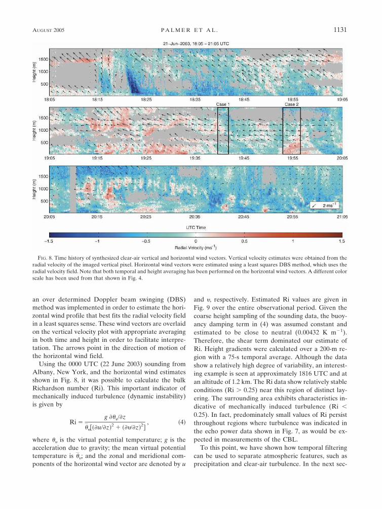
an over determined Doppler beam swinging (DBS)method was implemented in order to estimate the hori-zontal wind profile that best fits the radial velocity fieldin a least squares sense. These wind vectors are overlaidon the vertical velocity plot with appropriate averagingin both time and height in order to facilitate interpre-tation. The arrows point in the direction of motion ofthe horizontal wind field.

Using the 0000 UTC (22 June 2003) sounding fromAlbany, New York, and the horizontal wind estimatesshown in Fig. 8, it was possible to calculate the bulkRichardson number (Ri). This important indicator ofmechanically induced turbulence (dynamic instability)is given by

Ri �g ��z

��u��z�2 ��z�2�, �4�

where �� is the virtual potential temperature; g is theacceleration due to gravity; the mean virtual potentialtemperature is ��; and the zonal and meridional com-ponents of the horizontal wind vector are denoted by u

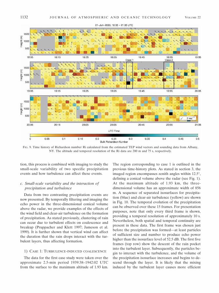
and �, respectively. Estimated Ri values are given inFig. 9 over the entire observational period. Given thecoarse height sampling of the sounding data, the buoy-ancy damping term in (4) was assumed constant andestimated to be close to neutral (0.00432 K m�1).Therefore, the shear term dominated our estimate ofRi. Height gradients were calculated over a 200-m re-gion with a 75-s temporal average. Although the datashow a relatively high degree of variability, an interest-ing example is seen at approximately 1816 UTC and atan altitude of 1.2 km. The Ri data show relatively stableconditions (Ri � 0.25) near this region of distinct lay-ering. The surrounding area exhibits characteristics in-dicative of mechanically induced turbulence (Ri �0.25). In fact, predominately small values of Ri persistthroughout regions where turbulence was indicated inthe echo power data shown in Fig. 7, as would be ex-pected in measurements of the CBL.

To this point, we have shown how temporal filteringcan be used to separate atmospheric features, such asprecipitation and clear-air turbulence. In the next sec-

FIG. 8. Time history of synthesized clear-air vertical and horizontal wind vectors. Vertical velocity estimates were obtained from theradial velocity of the imaged vertical pixel. Horizontal wind vectors were estimated using a least squares DBS method, which uses theradial velocity field. Note that both temporal and height averaging has been performed on the horizontal wind vectors. A different colorscale has been used from that shown in Fig. 4.


Fig 8 live 4/C

tion, this process is combined with imaging to study thesmall-scale variability of two specific precipitationevents and how turbulence can affect these events.

c. Small-scale variability and the interaction ofprecipitation and turbulence

Data from two contrasting precipitation events arenow presented. By temporally filtering and imaging theecho power in the three-dimensional conical volumeabove the radar, we provide examples of the effects ofthe wind field and clear-air turbulence on the formationof precipitation. As stated previously, clustering of raincan occur due to turbulent effects on coalescence andbreakup (Pruppacher and Klett 1997; Jameson et al.1999). It is further shown that vertical wind can affectthe duration that the rain drops interact with the tur-bulent layers, thus affecting formation.

1) CASE 1: TURBULENCE-INDUCED COALESCENCE

The data for the first case study were taken over theapproximate 2.5-min period 1939:38–1942:02 UTCfrom the surface to the maximum altitude of 1.93 km.

The region corresponding to case 1 is outlined in theprevious time-history plots. As stated in section 3, theimaged region encompasses zenith angles within 12.5°,defining a conical volume above the radar (see Fig. 1).At the maximum altitude of 1.93 km, the three-dimensional volume has an approximate width of 856m. A sequence of separated isosurfaces for precipita-tion (blue) and clear-air turbulence (yellow) are shownin Fig. 10. The temporal evolution of the precipitationcan be observed over these 15 frames. For presentationpurposes, note that only every third frame is shown,providing a temporal resolution of approximately 10 s.Nevertheless, both spatial and temporal continuity arepresent in these data. The first frame was chosen justbefore the precipitation was formed—at least particlesof sufficient size and number to produce echo powerhigher than the isosurface level of 52.5 dB. The first fiveframes (top row) show the descent of the rain pocketinto the turbulent layer. Subsequently, the particles be-gin to interact with the turbulence, and the volume ofthe precipitation isosurface increases and begins to de-scend through the layer. It is likely that the mixinginduced by the turbulent layer causes more efficient

FIG. 9. Time history of Richardson number Ri calculated from the estimated TEP wind vectors and sounding data from Albany,NY. The altitude and temporal resolution of the Ri data are 200 m and 75 s, respectively.


Fig 9 live 4/C

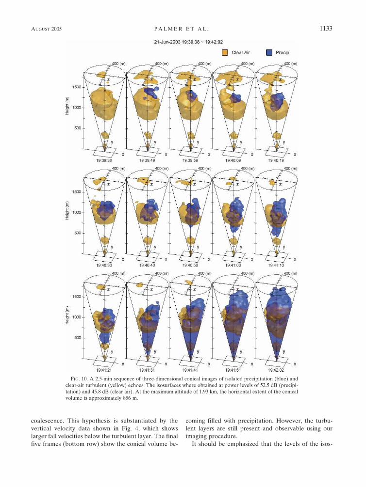
coalescence. This hypothesis is substantiated by thevertical velocity data shown in Fig. 4, which showslarger fall velocities below the turbulent layer. The finalfive frames (bottom row) show the conical volume be-

coming filled with precipitation. However, the turbu-lent layers are still present and observable using ourimaging procedure.

It should be emphasized that the levels of the isos-

FIG. 10. A 2.5-min sequence of three-dimensional conical images of isolated precipitation (blue) andclear-air turbulent (yellow) echoes. The isosurfaces where obtained at power levels of 52.5 dB (precipi-tation) and 45.8 dB (clear air). At the maximum altitude of 1.93 km, the horizontal extent of the conicalvolume is approximately 856 m.


Fig 10 live 4/C

urfaces (52.5 dB for precipitation, 45.8 dB for clear air)were chosen to study the interaction of these two dis-tinct signals. In the case of precipitation, it is possiblethat the volume was filled with relatively weak (lessthan 52.5 dB) rain signals, but these are not showngiven the chosen isosurface level. The flexibility of suchan analysis technique is evident. For example, it wouldeasily be possible to create a bank of bandpass tempo-ral filters, each with separate three-dimensional images.The center velocities of the filters could be chosen tospatially isolate particles of different fall velocities as aproxy for drop size (Palmer et al. 1998). Recent workby Worthington (2004) showed three-dimensional im-aging results similar to those of the present research butusing VHF (6-m wavelength) data from the MU radar.

2) CASE 2: TURBULENCE-INDUCED BREAKUP

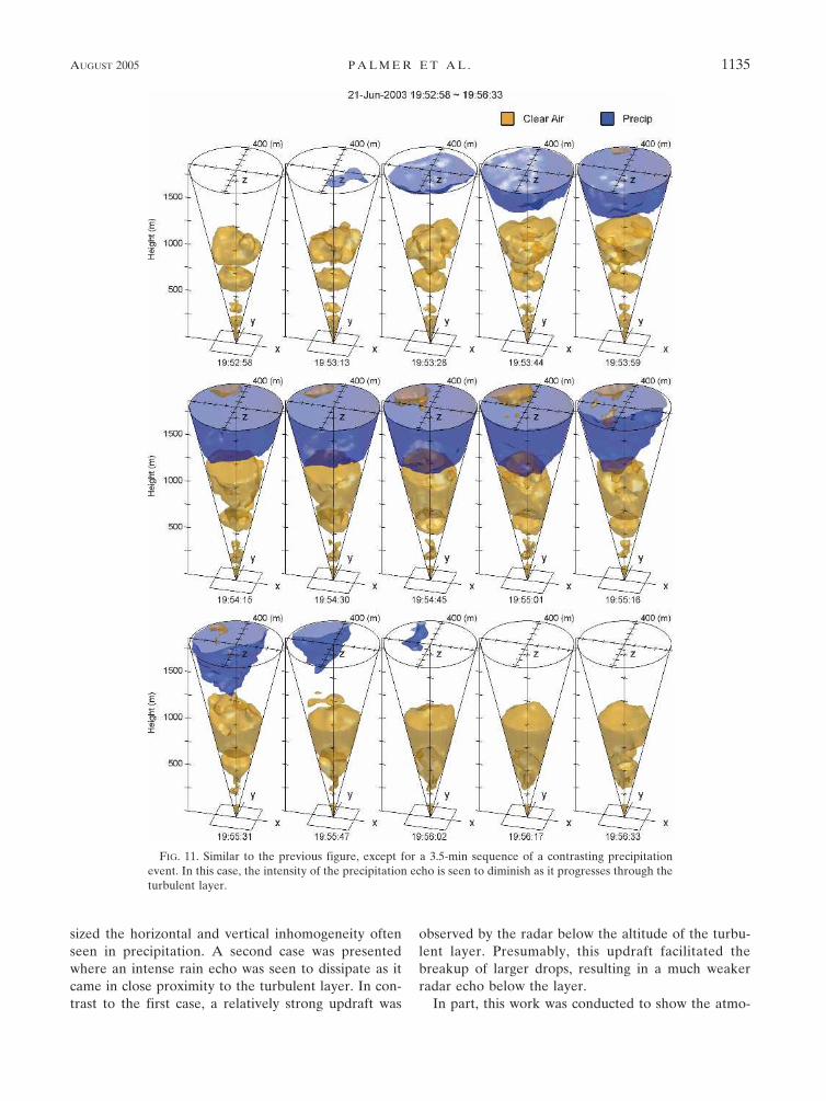
The second case study was derived from data takenduring the approximate 3.5-min period 1952:58–1956:33UTC over the same altitude range as in case 1. Forthese data, the temporal resolution was reduced to 15 sby presenting only every fourth frame, allowing studyof the entire precipitation event with reasonable pre-sentation quality. The sequence of three-dimensionalisosurfaces for both precipitation and clear air is pre-sented in Fig. 11. In the first five frames, an intenseprecipitation echo is seen to descend near the top of theturbulent layer at 1.2 km. The descent continues in thenext five frames, but as the precipitation begins to in-teract with the turbulent motion, the intensity of theecho diminishes. In the last five frames (bottom row)the precipitation isosurface dissipates, leaving only theclear-air turbulent echo. Why would the characteristicsof this event differ from those of case 1? By examiningthe time history of the clear-air wind profiles in Fig. 8,a reason for the difference can be ascertained. For thetime period corresponding to case 2, a significant up-draft (0.5 m s�1) is seen at 1955 UTC from the surfaceto approximately 500 m. This is in contrast to case 1, inwhich downward velocities dominated. It is likely thatthe upward velocities served to keep the raindrops aloftfor a longer duration than would have been the caseotherwise. This additional time allowed more interac-tion of the mixing processes of the turbulent layer, re-sulting in significant breakup of the larger drops. Thishypothesis is strengthened by studying the tilt of theprecipitation echoes in Fig. 6. At 1955 UTC and above1.5 km, the tilt is very steep, corresponding to large fallspeeds, or large drops. Below the turbulent layer, theprecipitation echo is only visible through our temporalfiltering process but shows a shallower slope, indicativeof small drops or drizzle. These smaller drops could becaused by turbulence-induced breakup. Of course, one

should be aware that the tilt of the precipitation echo isaffected by vertical motion, and any quantitative mea-sure of drop size, for example, would need to take thisinto account.

Other possible effects of updrafts on precipitationhave been noted by Kollias et al. (2001). In that work,the authors showed how upward motion in a convectivestorm could cause Doppler sorting, with larger dropsconcentrated toward the outer regions of the updraft.For our case of rather weak convective updrafts, how-ever, it is unlikely that such a sorting mechanism was atplay. Another possibility is that the updraft kept theraindrops aloft near a dry layer and evaporation causedthe observed effect. Water vapor measurements withthe necessary vertical resolution were not available totest this possibility. Nevertheless, evaporation shouldbe mentioned as one potential mechanism to explainthe observed characteristics.

The individual frames shown in Figs. 10 and 11 can beconsidered as instantaneous three-dimensional views ofthe structure within the transmit beam of the TEP ra-dar. It should be emphasized, however, that many ofthe features seen in the time sequence of images couldbe explained by advection. Given a nonzero horizontalwind, it is possible that horizontal inhomogeneity couldcause temporal variations in both the turbulent andprecipitation fields. Future work will attempt to addressthis issue by studying the effects of averaging time. Inessence, this will provide a mechanism to investigateTaylor’s frozen turbulence hypothesis using the TEPradar.

4. Conclusions

An experiment was conducted in June 2003 using the915-MHz TEP imaging radar in Amherst, Massachu-setts, for the purpose of studying the interaction of pre-cipitation and turbulence. The TEP radar is capable ofhigh-resolution observations of the boundary layer byimaging a conical volume above the radar defined bythe transmit beamwidth (�12.5°). The spatial resolu-tion was on the order of 30–40 m with a 5-s temporalresolution. During the experiment, sporadic liquid pre-cipitation occurred that was detected by the radar alongwith simultaneous clear-air turbulence echoes.

Using the distinct radial velocity signatures of pre-cipitation and clear-air turbulence, it was possible touse temporal filtering along with imaging to study theirsmall-scale interaction. Two contrasting case studieswere presented. In the first case, evidence was providedshowing an enhancement in coalescence when rela-tively light rain passed through a turbulent layer. Inaddition, three-dimensional imaging results empha-


sized the horizontal and vertical inhomogeneity oftenseen in precipitation. A second case was presentedwhere an intense rain echo was seen to dissipate as itcame in close proximity to the turbulent layer. In con-trast to the first case, a relatively strong updraft was

observed by the radar below the altitude of the turbu-lent layer. Presumably, this updraft facilitated thebreakup of larger drops, resulting in a much weakerradar echo below the layer.

In part, this work was conducted to show the atmo-

FIG. 11. Similar to the previous figure, except for a 3.5-min sequence of a contrasting precipitationevent. In this case, the intensity of the precipitation echo is seen to diminish as it progresses through theturbulent layer.


Fig 11 live 4/C

spheric research community the power of imaging radarsystems. With high spatial and temporal resolution, it ispossible to have a three-dimensional, virtual realityview of both precipitation and turbulence in the bound-ary layer. The 915-MHz TEP radar was developed bythe University of Massachusetts in the 1990s (Mead etal. 1998) and is undoubtedly one of the most sophisti-cated boundary layer radars in use today.

Acknowledgments. RDP, BLC, and MWH were sup-ported by the Army Research Office through GrantDDAD19-01-1-0407. SJF and FJL-D were supportedby the Army Research Office (Atmospheric Sciences)through Grant DAAG55-98-1-0480. The authors thankV. Tellabati for his work on the calibration of the TEParray.

REFERENCES

Capon, J., 1969: High-resolution frequency–wavenumber spec-trum analysis. Proc. IEEE, 57, 1408–1419.

Chau, J. L., and R. F. Woodman, 2001: Three-dimensional coher-ent radar imaging at Jicamarca: Comparison of different in-version techniques. J. Atmos. Sol.-Terr. Phys., 63, 253–261.

Cheong, B. L., M. W. Hoffman, R. D. Palmer, S. J. Frasier, andF. J. López-Dekker, 2004: Pulse pair beamforming and theeffects of reflectivity field variations on imaging radars. Ra-dio Sci., 39, RS3014, doi:10.1029/2002RS002843.

Chilson, P. B., C. W. Ulbrich, and M. F. Larsen, 1995: The effectsof particle size distributions on cross-spectral phase measure-ments in spatial interferometry. Radio Sci., 30, 1065–1083.

Cohn, S. A., 1995: Radar measurements of turbulent eddy dissi-pation rate in the troposphere: A comparison of techniques.J. Atmos. Oceanic Technol., 12, 85–95.

——, R. R. Rogers, S. Jascourt, W. L. Ecklund, D. A. Carter, andJ. S. Wilson, 1995: Interactions between clear-air reflectivelayers and rain observed with a boundary layer wind profiler.Radio Sci., 30, 323–341.

Crane, R. K., 1990: Space–time structure of rain rate fields. J.Geophys. Res., 95, 2011–2020.

Ecklund, W. L., D. A. Carter, and B. B. Balsely, 1988: A UHFwind profiler for the boundary layer: Brief description andinitial results. J. Atmos. Oceanic Technol., 5, 432–441.

Farley, D., H. Ierkic, and B. Fejer, 1981: Radar interferometry: Anew technique for studying plasma turbulence in the iono-sphere. J. Geophys. Res., 86, 1467–1472.

Fukao, S., T. Sato, T. Tsuda, S. Kato, K. Wakasugi, and T. Maki-hira, 1985a: The MU radar with an active phased array sys-tem, 1, Antenna and power amplifiers. Radio Sci., 20, 1155–1168.

——, T. Tsuda, T. Sato, S. Kato, K. Wakasugi, and T. Makihira,1985b: The MU radar with an active phased array system, 2,In-house equipment. Radio Sci., 20, 1169–1176.

Gossard, E. E., 1990: Radar research on the atmospheric bound-ary layer. Radar in Meteorology, D. Atlas, Ed., Amer. Me-teor. Soc., 477–527.

Gunn, R., and G. D. Kinzler, 1949: The terminal velocity of fallfor water drops in stagnant air. J. Meteor., 15, 452–461.

Haykin, S., 1985: Array Signal Processing. Prentice-Hall, 433 pp.Hélal, D., M. Crochet, H. Luce, and E. Spano, 2001: Radar im-

aging and high-resolution array processing applied to a clas-sical VHF-ST profiler. J. Atmos. Sol.-Terr. Phys., 63, 263–274.

Hocking, W. K., 1986: Observation and measurement of turbu-lence in the middle atmosphere with a VHF radar. J. Atmos.Terr. Phys., 48, 655–670.

Hysell, D. L., 1996: Radar imaging of equatorial F region irregu-larities with maximum entropy interferometry. Radio Sci., 31,1567–1578.

Jain, A. R., Y. J. Rao, P. B. Rao, V. K. Anandan, S. H. Damle, P.Balamuralidhar, A. Kulkarni, and G. Viswanathan, 1995: In-dian MST radar-Part II: First scientific results in ST mode.Radio Sci., 30, 1139.

Jameson, A. R., A. B. Kostinski, and A. Kruger, 1999: Fluctuationproperties of precipitation. Part IV: Finescale clustering ofdrops in variable rain. J. Atmos. Sci., 56, 82–91.

Kollias, P., B. A. Albrecht, and J. F. D. Marks, 2001: Raindropsorting induced by vertical drafts in convective clouds. Geo-phys. Res. Lett., 28, 2787–2790.

Kudeki, E., and R. Woodman, 1990: A poststatistics steering tech-nique for MST radar applications. Radio Sci., 25, 591–594.

——, and F. Sürücü, 1991: Radar interferometric imaging of field-aligned plasma irregularities in the equatorial electrojet.Geophys. Res. Lett., 18, 41–44.

——, B. G. Fejer, D. T. Farley, and H. M. Ierkic, 1981: Interfer-ometer studies of equatorial F region irregularities and drifts.J. Geophys. Res., 8, 377–380.

Lopez-Dekker, P. L., and S. J. Frasier, 2004: Radio acousticsounding with a UHF volume imaging radar. J. Atmos. Oce-anic Technol., 21, 766–776.

Luce, H., M. Crochet, and F. Dalaudier, 2001: Temperature sheetsand aspect sensitive radar echoes. Ann. Geophys., 19, 899–920.

Mead, J. B., G. Hopcraft, S. J. Frasier, B. D. Pollard, C. D.Cherry, D. H. Schaubert, and R. E. McIntosh, 1998: A vol-ume-imaging radar wind profiler for atmospheric boundarylayer turbulence studies. J. Atmos. Oceanic Technol., 15, 849–859.

Palmer, R. D., M. F. Larsen, E. L. Sheppard, S. Fukao, M. Yama-moto, T. Tsuda, and S. Kato, 1993: Poststatistic steering windestimation in the troposphere and lower stratosphere. RadioSci., 28, 261–271.

——, S. Gopalam, T. Yu, and S. Fukao, 1998: Coherent radarimaging using Capon’s method. Radio Sci., 33, 1585–1598.

Pfister, W., 1971: The wave-like nature of inhomogeneities in theE-region. J. Atmos. Terr. Phys., 33, 999–1025.

Pollard, B. D., S. Khanna, S. J. Frasier, J. C. Wyngaard, D. W.Thomson, and R. E. McIntosh, 2000: Local structure of theconvective boundary layer from a volume-imaging radar. J.Atmos. Sci., 57, 2281–2296.

Pruppacher, H. R., and J. D. Klett, 1997: Microphysics of Cloudsand Precipitation. 2d ed. Kluwer Academic Press, 954 pp.

Rao, P. B., A. R. Jain, P. Kishore, P. Balamuralidhar, S. H.Damle, and G. Viswanathan, 1995: Indian MST radar-Part I:System description and sample vector wind measurements inST mode. Radio Sci., 30, 1125.

Röttger, J., and H. Ierkic, 1985: Postset beam steering and inter-ferometer applications of VHF radars to study winds, waves,and turbulence in the lower and middle atmosphere. RadioSci., 20, 1461–1480.

Tatarskii, V. I., 1961: Wave Propagation in a Turbulent Medium.McGraw-Hill, 285 pp.

Vaillancourt, P. A., and M. K. Yau, 2000: Review of particle–


turbulence interactions and consequences for cloud physics.Bull. Amer. Meteor. Soc., 81, 285–298.

Wakasugi, K., A. Mizutani, M. Matsuo, S. Fukao, and S. Kato,1986: A direct method for deriving drop-size distribution andvertical air velocities from VHF Doppler radar spectra. J.Atmos. Oceanic Technol., 3, 623–629.

Weber, B. L., and Coauthors, 1990: Preliminary evaluation of thefirst NOAA demonstration network wind profiler. J. Atmos.Oceanic Technol., 7, 909–918.

Woodman, R. F., 1971: Inclination of the geomagnetic field mea-sured by an incoherent scatter technique. J. Geophys. Res.,76, 178–184.

——, 1997: Coherent radar imaging: Signal processing and statis-tical properties. Radio Sci., 32, 2373–2391.

——, and A. Guillen, 1974: Radar observations of wind and tur-bulence in the stratosphere and mesosphere. J. Atmos. Sci.,31, 493–505.

Worthington, R. M., 2004: All-weather volume imaging of theboundary layer and troposphere using the MU radar. Ann.Geophys., 22, 1407–1419.

Yu, T.-Y., R. D. Palmer, and D. L. Hysell, 2000: A simulationstudy of coherent radar imaging. Radio Sci., 35, 1129–1141.

——, ——, and P. B. Chilson, 2001: An investigation of scatteringmechanisms and dynamics in PMSE using coherent radarimaging. J. Atmos. Sol.-Terr. Phys., 63, 1797–1810.


observations of the small-scale variability of …boonleng/pdf/palmer++05.pdfobservations of the...

Documents