Observations on the Dynamics of a Congestion Control Algorithm: The Effects

of Two-Way Traffic

Lixia Zhang Scott Shenker David D. Clark

Computer Science Laboratory Laboratory for Computer Science

Xerox Palo Alto Research Center Massachusetts Institute of Technology

Abstract

We use simulation to study the dynamics of the congestioncent rol algorithm embedded in the BSD 4.3-Tahoe TCP im-

plementation. We investigate the simple case of a few TCPconnections, originating and terminating at the same pair of

hosts, using a single bottleneck link. This work is an exten-sion of our earlier work ([16]), where one-way traffic (i.e., all

of the sources are on the same host and all of the destina-tions are on the other host) was studied. In this paper we

investigate the dynamics that results from two-way traffic(in which there are data sources on both hosts). We find

that the one-way traffic clustering and loss-synchronizationphenomena d~cussed in [16] persist in this new situation,

albeit in a slightly modified form. In addition, there aretwo new phenomena not present in the earlier study: (1)

ACK-compression, which is due to the interaction of dataand ACK packets and gives rise to rapid fluctuations in

queue length, and (2) an out-of-phase queue-synchronizationmode, which keeps link utilization less than optimal even in

the limit of very large buffers. These phenomena are helpfulin understanding results from an earlier study of network

oscillations ([19]).

1 Introduction

One of the longstanding problems with datagram networks

is that it is difficult to control congestion. However, in thepaat decade, tremendous progress has been made on this

problem. One particularly noteworthy success is the conges-tion control algorithm developed by Jacobson ([6]), which is

currently embedded in the BSD 4.3-Tahoe TCP implemen-tation and is similar in spirit to the one Jain, Ramakrishnan,

and Chiu ([8]) designed for the DECnet architecture. Jacob-son’s congestion control algorithm has resulted in a dramatic

reduction in congestion in the Internetl and has become anInternet standard ([1]). Thus, it is important to understandthe behavior of this algorithm. We hope that increased in-sight into this particular algorithm can both lead to betterunderstanding of the behavior of the current Internet and

1While we are not aware of anyone who disputes this statement,

the evidence for improved overall Internet performance due to this

congestion control algorithm is mostly anecdotal.

Permission to copy without fee all or part of this material is

granted provided that the copies are not made or distributed for

direct commercial advantage, the ACM copyright notice and the

title of the publication and its date appear, and notice is given

that copying ia by permission of the Association for Computing

Machinery. To copy otherwise, or to republish, requirss a fae

and/or spacific permission.Q 1991 ACM 0.89791.444-9/91 /@xj8\0J 33... $1 .~()

provide guidance for the design of new congestion control

algorithms.While the practical benefits of this congestion control al-

gorithm are clear, its behavior is not yet fully understood.There is a small, but rapidly growing, set of simulation stud-ies of this algorithm; for example, see [2, 3, 4, 5, 10, 16, 18,19]. In several of these studies the focus is on the effectof various gateway disciplines such as Fair Queueing ([2, 3])and Random Drop ([4, 5, 10, 18]) on network performance in

the presence of traffic sources using the BSD 4.3-Tahoe TCPcongestion control algorithm. Several other studies ([5, 18])

present aggregate throughput, loss, and delay characteristicsof this congestion control algorithm in various complicated

network configurations.In contraat, in this paper we examine only a few sim-

ple network configurations with standard FIFO gateways.

Our focus is instead on the detailed dynamics of the conges-tion control algorithm in rather simple settings. Aside from

the seminal work of Jacobson [6], these dynamics have re-

ceived little attention. Some aspects of these dynamics werestudied in [19], where simulations on two different network

configurations revealed the presence of rapid queue lengthfluctuations. While preliminary explanation were offered,

the complexity of the network configurations precluded asystematic analysis. One of the purposes of this paper is toreproduce the essential elements of that fluctuating behav-ior in the simplest possible network configuration so that it

can be more fully analyzed.This paper is a continuation of the research effort initi-

ated in [16]. There we examined the dynamics of the BSD

4.3-Tahoe TCP congestion control algorithm in the simplest

of network configurations: one or several TCP connections,originating and terminating at the same pair of hosts, send-

ing traffic through a single bottleneck link, with all of theconnections transmitting in the same direction (i.e., with allof the sources of the connections on one host and all of the

destinations of the connections on the other host). Sinceall of the data packets travel in one direction and all of theACK packets travel in the other, the dynamics are relativelytractable in this configuration. In the present paper, we re-

tain the same network topology of a single bottleneck linkbut progress to the slightly more complicated situation ofhaving one source on each host, so that both data and ACKpackets travel in each direction. The seemingly innocuous

modification of introducing two-way traffic greatly compli-cates the dynamite. More surprisingly, it appears that allof the essential elements of the behavior reported in [19] are

present in this simple configuration.

133

In the one-way traffic configuration, there are two rto-table aapects of the behavior: the clustering of packets from

each connection and the synchronization of packet losses(these effects will be described in more detail later). Two-way traffic exhibits similar phenomena. However, there are

two dynamic phenomena that are singular to two-way traf-

fic. The first, labeled ACK-compression, gives rise to rapidfluctuations in the queue length at the bottleneck gateway.In contrast to one-way traffic, where the ACK’S provide areliable clock to regulate traffic and keep the queue length

variations modest, in t we-way traffic the ACK’s can become

compressed together and hence lose their clocking proper-ties. The second phenomenon is an out-of-phase synchro-nization mode. In the one-way traffic configuration, all of

the connections are synchronized in-phase in that the flowcontrol windows of the various connections all increase and

decrease at the same time. With two-way traffic, under cer-tain conditions the connections in different directions are

synchronized out-of-phase in that the flow control windowof one connection is increasing while that of the other is

decreasing. This phenomenon has the effect of keeping thebottleneck utilization below optimal, even in the limit of

infinite buffers.Our detailed analysis is only applicable to the single spe-

cific network configuration we consider. However, the basicphenomena of ACK-compression and synchronization modes

seem to be present iu the dynamics of much more compli-cated configurations. Similarly, while the present study is

limited to investigating the behavior of one specific conges-tion control algorithm, we think that the effects described

above apply to a wider class of algorithms. In fact, we con-

jecture that any nonpacedz window-based congestion controlalgorithm will exhibit these two phenomena.

We hasten to note, however, that our study is rather in-complete. The BSD 4.3-Tahoe TCP congestion control al-

gorithm gives rise to a wealth of complicated dynamical be-havior; we have only examined the most accessible of these.Even in the extremely simple configurations examined here,there are effects that we do not yet fully understand. More

importantly, for those behaviors which we do understand, we

have yet to determine how relevant the insight gained from

examining relatively simple network topologies is to morecomplicated and realistic network configurations. This is

the subject of future work.This paper has 6 sections. In the next section, we briefly

describe the BSD 4.3-Tahoe TCP congestion control algo-rithm and discuss our network model and simulator. Toprovide context for the two-way traffic simulations presentedhere, in Section 3 we review the one-way traffic results from

[16] and the rapid queue length fluctuation results from [19].

In Section 4 we examine the novel behavioral amects of two-.way traffic, focusing on ACK-compression and synchroniza-tion modes. The relationship between this data and that

iu [19] and the effect of various other factors, such as thedelayed-ACK option and other network topologies, are dis-cussed in Section 5. We summarize our results in Section 6.

2 Pacing will be discussed later, but for now it suffices to define

a nonpaced algorithm ss one in which the source sends data packets

immediately upon the receipt of an ACK, without introducing any

artificial delay which would spread out packets.

2 Network: Algorithm, Configuration, and Simulator

In this section we first give a brief overview of the BSD 4.3-Tahoe TCP congestion control algorithm, then discuss thenet work configurations considered, and lastly describe the

network simulator used.

2.1 BSD 4.3-Tahoe TCP Congestion Control Algorithm

The followiug is a very abbreviated and oversimplified de-

scription of the BSD 4.3-Tahoe TCP congestion control al-gorithm. For further details, see either [6] or the BSD 4.3-Tahoe code itself (which has sufficient comments to render

it a useful text). At TCP connection set-up the receiverspecifies a maximum window size mazwnd.3 To simplifythe presentation in this paper, we will assume that all win-

dow sizes are measured in units of maximum size packets,

instead of bytes. In the original TCP specification ([14]), thewindow used by the sender, which we will denote by wnd,

is the receiver advertised window max wnd regardless of theload in the network. In the BSD 4.3-Tahoe TCP algorithm,

the window size used by the sender is adjusted in responseto network congestion. The sender has a variable called the

congestion window cwnd, which is increased whenever newdata is acknowledged and decreased whenever a packet loss

is detected.4 The actual window used by the sender is thefloor of the minimum of the congestion window and the re-

ceiver advertised window:5wnd = lMIN(cwnd, maxwnd)]

The congestion window adjustment algorithm haa twophases, the slow-start or congestion recovery phase, where

the window is increased rapidly, and the congestion avoid-ance phase, where the window is increased much more slowly.

A control threshold, ssthresh, determines which phase aconnection is in. Whenever a packet drop is detected, ssthresh

is set to half of the current cwnd value, cwnd is then set toone, and the congestion recovery phase begins. cwnd in-creases rapidly until it passes the threshold ssthresh, thenthe algorithm switches into the congestion avoidance phase.

The specifics of the adjustment algorithm in the real BSD4.3-Tahoe TCP code are as follows:

When new data is acknowledged, the sender does

if (cvnd < ssthresh)

cvnd += 1;else

cvnd += 1 / crmd

When a packet drop is detected, the sender does

ssthresh = MAX [ MIN (cund/2, maxvnd), 2]

cund = 1

We define an epoch of a TCP connection to be the time

period during which an entire window’s worth of packetshave been acknowledged. We will focus particularly on thoseepochs in which packet losses occur. These will be calledcongestion epochs.

The amount by which the congestion window increasesduring an epoch, which we will call the acceleration, is an

3 The variable names used here are not the same as in the BSD

4.3-Tahoe code.

4 Packet losses are detected by either the receipt of duplicate ac-

knowledgments or the expiration of a timer.

5 Since TCP transmits maximum size packets whenever possible to

avoid the silly-window syndrome, w n d will always be an integer and

is the maximum number of outstanding packets allowed.

134

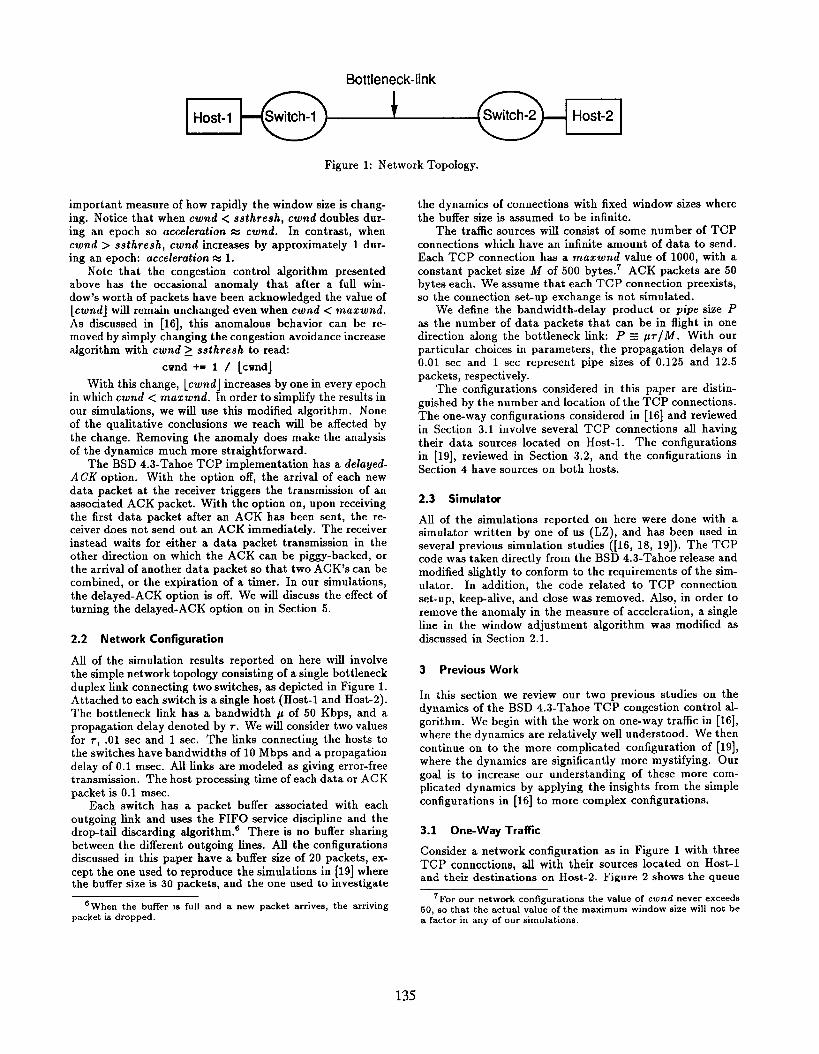
Bottleneck-link

Host-1 1 Host-2

Figure 1: Network Topology.

important measure of how rapidly the window size is chang-

ing. Notice that when cwnd < ssthretrh, cwnd doubles dur-

ing an epoch so acceleration = cwnd. In cent rast, whencwnd > sstlwesh, cwnd increases by approximately 1 dur-

ing an epoch: acceleration = 1.

Note that the congestion control algorithm presentedabove has the occasional anomaly that after a full win-dow’s worth of packets have been acknowledged the value of[cwnd] will remain unchanged even when cwnd < maxwnd.

As discussed in [16], this anomalous behavior can be re-moved by simply changing the congestion avoidance increase

algorithm with cwnd ~ ssthresh to read:

cwnd += 1 / lcvnd]

With this change, lcwndJ increases by one in every epoch

in which cwnd < maz w nd. In order to simplify the results in

our simulations, we will use this modified algorithm. Noneof the qualitative conclusions we reach will be affected by

the change. Removing the anomaly does make the analysisof the dynamics much more straightforward.

The BSD 4.3-Tahoe TCP implementation has a delayed-A CK option. With the option off, the arrival of each new

data packet at the receiver triggers the transmission of anassociated ACK packet. With the option on, upon receivingthe first data packet after an ACK has been sent, the re-ceiver does not send out an ACK immediately. The receiver

instead waits for either a data packet transmission in theother direction on which the ACK can be piggy-backed, or

the arrival of another data packet so that two ACK’S can becombined, or the expiration of a timer. In our simulations,

the delayed-ACK option is off. We will discuss the effect ofturning the delayed-ACK option on in Section 5.

2.2 Network Configuration

All of the simulation results reported on here will involvethe simple network topology consisting of a single bottleneck

duplex link connecting two switches, as depicted in Figure 1.Attached to each switch is a single host (Host-1 and Host-2).

The bottleneck link has a bandwidth p of 50 Kbps, and apropagation delay denoted by ~. We will consider two values

for r, .01 sec and 1 sec. The links connecting the hosts tothe switches have bandwidths of 10 Mbps and a propagation

delay of 0.1 msec. All links are modeled as giving error-freetransmission. The host processing time of each data or ACK

packet is 0.1 msec.Each switch has a packet buffer associated with each

outgoing link and uses the FIFO service discipline and thedrop-tail discarding algorithm.e There is no buffer sharing

between the different outgoing lines. All the configurationsdiscussed in this paper have a buffer size of 20 packets, ex-

cept the one used to reproduce the simulations in [19] wherethe buffer size is 30 packets, and the one used to investigate

6 When the buffer is full and a new packet arrives, the arriving

packet is dropped.

the dynamics of connections with fixed window sizes where

the buffer size is assumed to be infinite.The traffic sources will consist of some number of TCP

connections which have an infinite amount of data to send.Each TCP connection has a maxwnd value of 1000, with a

constant packet size M of 500 bytes. 7 ACK packets are 50bytes each. We assume that each TCP connection preexists,

so the connection set-up exchange is not simulated.We define the bandwidth-delay product or pipe size P

as the number of data packets that can be in flight in onedirection along the bottleneck link: P s pr/M. With our

particular choices in parameters, the propagation delays of0.01 sec and 1 sec represent pipe sizes of 0.125 and 12.5packets, respectively.

The configurations considered in this paper are distin-

guished by the number and location of the TCP connections.The one-way configurations considered in [16] and reviewed

in Section 3.1 involve several TCP connections all having

their data sources located on Host-1. The configurationsin [19], reviewed in Section 3.2, and the configurations in

Section 4 have sources on both hosts.

2.3 Simulator

All of the simulations reported on here were done with asimulator writ ten by one of us (L Z), and has been used in

several previous simulation studies ([16, 18, 19]). The TCPcode was taken directly from the BSD 4.3-Tahoe release and

modified slightly to conform to the requirements of the sim-ulator. In addition, the code related to TCP connectionset-up, keep-alive, and close was removed. Also, in order to

remove the anomaly in the measure of acceleration, a singleline in the window adjustment algorithm was modified as

d~cussed in Section 2.1.

3 Previous Work

In this section we review our two previous studies on thedynamics of the BSD 4.3-Tahoe TCP congestion control al-

gorithm. We begin with the work on one-way traffic in [16],where the dynamics are relatively well understood. We then

continue on to the more complicated configuration of [19],where the dynamics are significantly more mystifying. Our

goal is to increase our understanding of these more com-plicated dynamics by applying the insights from the simple

configurations in [16] to more complex configurations.

3.1 One-Way Traffic

Consider a network configuration as in Figure 1 with three

TCP connections, all with their sources located on Host-1and their destinations on Host-2. Figure 2 shows the queue

7For ~“r network configurations the value of cw n d never ‘Xceeds

50, so that the actual value of the maximum window size will not bea factor in any of our simulations.

135

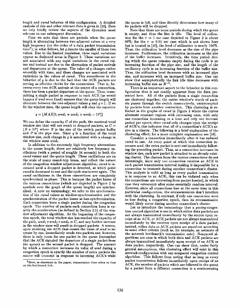
length and cwnd behavior of thk configuration, A detailedanalysis of this and other relevant data is given in [16]. Herewe only briefly review the aspects of the dynamics mostrelevant to our subsequent discussion.

First we note that there are periods when the queuelength is alternating between two adjacent values at a veryhigh frequency (on the order of a data packet transmissiontimes ); in what follows, let q denote the smaller of these two

values. Due to the limited resolution, these rapid variationsappear as darkened areas in Figure 2. These variations arenot associated with any rapid variations in the cwnd val-

ues and instead are due to the alternation of packet arrivals

and departures at the queue. The value of q changes rathersmoothly with time, and these changes are associated with

variations in the values of cwnd. This smoothness in thebehavior of q is due to the fact that the ACK packets areserving as effective clocks for the connections. That is, be-

tween every two ACK arrivals at the source of a connection,there has been a packet departure at the queue. Thus, trans-

mitting a single packet in response to each ACK (as would

happen if wnd were fixed) ensures that the queue length willalternate between the two adjacent values g and g +1. If we

fix the window sizes, the queue length will obey the equation

q = [&lAX[O, wndl + wndz + wndt – 2P]]

We can define the capacity C of the path, the maximal totalwindow size that will not result in dropped packets, as C =

[B+ 2P] where B is the size of the switch packet buffer

and P is the pipe size. Since q is a function of the totalwindow size, each change in q is associated with a change inthe window sizes wndi.

In addition to the extremely high frequency alternationsin the queue length, there are relatively low frequency os-

cillations (with a period of roughly 34 seconds) in both thecwnd values and the queue length. These oscillations are on

the scale of many round-trip times, and reflect the natureof the congestion window adjustment algorithm; cwnd is in-creased until a dropped packet is detected, at which pointcwnd is decreased to one and the cycle starts over again. The

cwnd os@lations in the three connections are completely

synchronized in-phase. This is because the packet losses of

the various connections (which are depicted in Figure 2 bysymbols over the graph of the queue length) are synchr~

nized. A note on terminology; we refer to the synchronizetion of the cwnd values as window-synchronization and thesynchronization of the packet losses as loss-synchronization.Each connection loses a single packet during the congestion

epoch. The number of packets each connection loses is ex-actly the acceleration (as defined in Section 2.1) of the win-

dow adjustment algorithm. At the beginning of the conges-tion epoch, the total window size has reached the capacity of

the path, wndl +wndz+wndt = C, and any further increasein the window sizes will result in dropped packets. A source,upon receiving the AGK that causes the value of wnd to in-crease by one, immediately sends two packets out; however,there is only room for one packet in the queue (rememberthat the ACK signaled the departure of a single packet fromthe queue) so the second packet is dropped. The amountby which a connection increases its value of wnd during a

congestion epoch is exactly the number of extra packets thesource will transmit in response to incoming ACK’S while

sHere W elsewhere in the paper, transmission time refers to thaton the bottleneck link.

the queue is full, and thus directly determines how many ofits packets will be dropped.

Note that there are some periods during which the queueis empty, and thus the line is idle. The level of utilizw

tion for the r = 1 sec case depicted in Figure 2 is about9070; for the r = 0.01 sec case which is not shown here

but is treated in [16], the level of utilization is nearly 100%.

Thus, the utilization level decrerwes as the size of the pipeincreases. Furthermore, the utilization increases as the sizeof the buffer increwes. Intuitively, the time period dur-ing which the queue remains empty during the cycle is an

increasing function of the pipe size, and the length of the

oscillatory cycle is an increasing function of the buffer size.Thus, the utilization level decreases with an increased pipe

size, and increases with an increased buffer size. One canshow that asymptotically the link idle time decreases with

increasing buffer size as B-2.

There is an important aspect to the behavior in thk con-figuration that is not readily apparent from the data pre-sented here. All of the packets from a single connection

are clustered together; the entire window’s worth of pack-ets passes through the switch consecutively, uninterruptedby packets from another connection. This clustering is re-flected in the graphs of cwnd in Figure 2 where the curves

alternate constant regions with increasing ones, with onlyone connection increasing at a time and only one increase

period per epoch; since cwnd only changes upon the receiptof ACK ‘s, this indicates that all of a connection’s ACK’s ar-

rive in a cluster. The following is a brief explanation of theclustering effect; for a more complete explanation see [16].

Consider a connection immediately after it has reducedcwnd to one. At every point at which this connection in-

creases wnd, the extra packet is sent out immediately follow-

ing the preceding packet. Thus, as a connection increases itswindow size, each new packet is attached to an already exist-

ing cluster. The clusters from the various connections do notintermingle, since only one connection receives an ACK in

each packet transmission interval making it impossible for aconnection to transmit during another connection’s cluster.This analysis is valid as long as every packet transmissionis in response to an ACK; this can be violated only when

the connections are recovering from packet loss(es), in which

case they retransmit after some essentially random interval.

However, since all connections lose at the same time in this

particular configuration, the retransmissions don’t interfere

with the clustering. In contrast, if only one connection wereto lose during a congestion epoch, then its retransmissionwould likely occur during another connection’s cluster.

Let us introduce the terminology that a pacing conges-tion control algorithm is one in which either data packets arenot always transmitted immediately by the source upon re-ceipt of an ACK, or ACK packets are not always transmittedimmediately by the receiver upon receipt of a data packet;

instead, either data or ACK packets are paced out accordingto some other criteria (such as, for example, an estimate ofthe net work bottleneck’s transmission rate). Nonpaced al-gorithms are ones in which both data and ACK packets are

always transmitted immediately upon receipt of an ACK ordata packet, respectively. One can show that, under fairly

general assumptions, this clustering effect will exist in th~

network configuration with any nonpaced congestion controlalgorithm. This follows from noting that as long as everypacket transmission follows immediately upon receipt of anACK, the number of packets which are followed in the queueby a packet from a different connection is a nonincreasing

136

Z5

20

15

70

5

0

.*. .*.

T1 -cross, T2-star, T3-bOx

.*.

240 Zb Zho 3bo 3>0Clock(soc)

T 1-solid, T2-dashexl, T3-dot@d

o I

Z& 21?0 220 260 Zi?o 300 320Clock(sec)

Figure 2: Packet queue at the switch and congestion window sizes for a configuration with three connections, all having

sources on Host-1, and with ~ = 1 sec. The swit~hes have a buffer size of 20 packets. The marks above the graph oft he queuelength show the times when packets from the various connections are dropped; the darkened regions are due to the queue

length alternating between two adjacent values as packets arrive and depart in an interleaved fashion.

function. Experimentally, the same clustering effect hasbeen reported ([11]) in a very different congestion control

algorithm (see [12] for a description). Note, however, thatthe analysis of the clustering effect depends in detail on theround-trip times of the various connections being identical.See Section 5 for further discussion of this point.

While we cannot claim to fully understand every detail

of the dynamics in this configuration, most of the relevant

phenomena here do seem comprehensible within the frame-

work we developed in [16]. A natural progression to morecomplicated configurations would lead to consideration of

having the sources of the TCP connections located on bothhosts. Such a configuration was considered in [19], to which

we now turn.

3.2 Rapid Queue Fluctuations

Reference [19] discussed the dynamics in two network con-

figurations significantly more complicated than the one dis-cussed in [16] which was reviewed above. The simpler of

the two configurations considered in [19] is similar to that of

Figure 1 with ten TCP connections, five having their sourceon Host-1 and five having their source on Host-2. The ac-tual configuration considered in [19] had somewhat differ-

ent line speeds, and did not use the slight modification tothe congestion control algorithm (described in Section 2.1),

but those differences have no qualitative impact on the re-sults. To facilitate direct comparisons, we have chosen to

show simulation results from such a configuration based on

the network in Figure 1 with T = 0.01 sec and the conges-tion cent rol algorithm described in Section 2.1 rather than

reproducing the data from the original paper. In this con-figuration, both switches have a buffer size of 30 packets.

The graphs of the total queue length at the two switches areshown in Figure 3.

The data bears some resemblance to that for the pre-vious configuration. The queue lengths still exhibit a low

frequency oscillation. However, the most striking feat ure ofthis data is the rapid fluctuations in the queue size. The

fluctuations are on the order of 5 packets and occur on atime scale smaller than that of a single data packet trans-

mission time. These fluctuations are not associated withcorrespondingly large changes in the cwnd values. This be-havior is in sharp contrast to what we saw in the one-way

traffic case, where the queue length varied smoothly. Theserapid fluctuations in queue length are the central mystery

of the dynamics of this configuration.

Another intriguing aspect to the behavior is that there issignificant idle time on the bottleneck lines even though thepipe P is quite small. The utilization on the line is roughly91Y0, compared to nearly 100~o utilization with only one-way traffic. Furthermore, when one increases the buffer size

137

Clock(sec)

20- W II

w

1s -

To - 4

ml

s-

0 ‘1 Illllu 11111t

SZo S2S S30 535 S40 545 SsoCIock(sec)

Figure 3: Packet queue at switches 1 and 2 for a configuration with ten connections, five having their source on Host-1 and

five having their source on Host-2, with T = 0.01 sec. The switches have a buffer size of 30 packets.

the fraction of idle time does not decrease; in fact when

the buffer size is increased to 60 the utilization decreases toroughly 87~0. In one way traflic, there is significant idle time

only when P is large and, for any given P, the fraction ofidle time asymptotically vanishes in the limit of large buffers.

This one-way behavior has given rise to the commonly-heardassertion that increasing buffers is a reliable way to increasethroughput. The data here contradicts that assertion.

One issue that arises only when there are two congestedqueues, rather than the single congested queue in the one-way traffic case, is the relative synchronization of the queue

lengths in the two switches. In Figure 3 the queue lengthsboth go through similar low frequency oscillations, but they

are out-of-phase with each other. One queue reaches its

maximum while the other queue is at its minimum.

For the sake of brevity, we have not shown any data onthe cwnri or packet-drop behavior, which are not nearly sosimply characterized as in the one-way traffic case; we nowbriefly summarize those results. There is still some degreeof loss-synchronization, in that the majority of the connec-tions lose packets during the same congestion epoch. Oneremarkable occurrence is that 99.8~0 of the dropped pack-

ets are data packets, even though during a congestion epochall connections are sending packets to a nearly full queuewith some of the packets being data packets and some be-ing ACK packets. Since only one of the two queues is fullduring a congestion epoch (the other is nearly empty), thistendency to drop only data packets implies that only con-

nections sending data packets through the congested queueexperience drops during that congestion epoch. In addition,the cwnd data indicates that the connections sending in the

same direction are window-synchronized in-phase, but the

connections with sources on Host-1 are synchronized out-

of-phase with the connections on Host-2. This is reflectedin the out-of-phase synchronization of the queue behaviordiscussed above. The total number of packet drops per con-

gestion epoch varies, but the average is approximately ten,the same as the total acceleration in this configuration.

It is clear that the insights gained in [16] are not suffi-

cient to explain the behavior in this more complicated con-figuration. However, the presence of ten connections makes

a detailed analysis difficult. Thus it seems natural to con-sider the simplest cae.e of two-way traffic: that of two TCP

connections with sources on different hosts. The dynamicsof that configuration is the focus of the rest of this paper.

4 Features of Two-Way Traffic

In this section we analyze the dynamics of the configurationconsisting of a network as in Figure 1 with two connections,connection 1 having its source on Host-1 and connection2 having its source on Host-2. We present our analysis in

three parts. We first give an overview of the dynamics, thenexamine more closely the phenomena of ACK-compressionand synchronization modes.

138

4.1 Overview

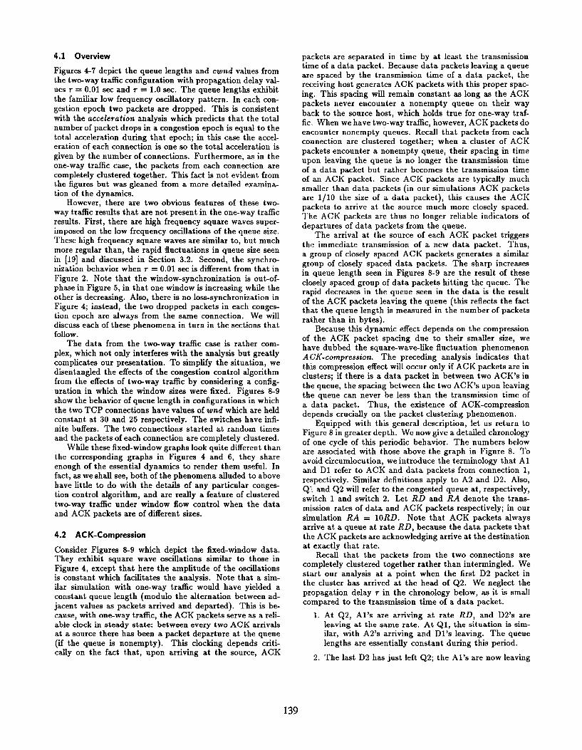
Figures 4-7 depict the queue lengths and cwnd values fromthe two-way traffic configuration with propagation delay val-ues T = 0.01 sec and T = 1.0 sec. The queue lengths exhibit

the familiar low frequency oscillatory pattern. In each con-

gestion epoch two packets are dropped. This is consistent

with the acceleration analysis which predicts that the total

number of packet drops in a congestion epoch is equal to thetotal acceleration during that epoch; in this case the accel-eration of each connection is one so the total acceleration is

given by the number of connections. Furthermore, as in theone-way traffic case, the packets from each connection are

completely clustered together. This fact is not evident fromthe figures but was gleaned from a more detailed examina-

tion of the dynamics.However, there are two obvious features of these two-

way traffic results that are not present in the one-way traffic

results. First, there are high frequency square waves super-imposed on the low frequency oscillations of the queue size.These high frequency square waves are similar to, but much

more regular than, the rapid fluctuations in queue size seen

in [19] and discussed in Section 3.2. Second, the synchro-nization behavior when r = 0.01 sec is different from that in

Figure 2. Note that the window-synchronization is out-of-phase in Figure 5, in that one window is increasing while the

other is decreasing. Also, there is no loss-synchronization inFigure 4; instead, the two dropped packets in each conges-tion epoch are always from the same connection. We willdiscuss each of these phenomena in turn in the sections thatfollow.

The data from the two-way trailic case is rather com-

plex, which not only interferes with the analysis but greatlycomplicates our presentation. To simplify the situation, wedisentangled the effects of the congestion control algorithm

from the effects of tw-way traffic by considering a config-

uration in which the window sizes were fixed. Figures 8-9

show the behavior of queue length in configurations in which

the two TCP connections have values of wnd which are heldconstant at 30 and 25 respectively. The switches have infi-

nite buffers. The two connections started at random timesand the packets of each connection are completely clustered.

While these fixed-window graphs look quite different thanthe corresponding graphs in Figures 4 and 6, they share

enough of the essential dynamics to render them useful. Infact, as we shall see, both of the phenomena alluded to above

have little to do with the details of any particular conges-tion control algorithm, and are really a feature of clustered

two-way traffic under window flow control when the data

and ACK packets are of different sizes.

4.2 AC K-Compression

Consider Figures 8-9 which depict the fixed-window data.They exhibit square wave oscillations similar to those in

Figure 4, except that here the amplitude of the oscillationsis constant which facilitates the analysis. Note that a sim-

ilar simulation with one-way traffic would have yielded aconstant queue length (modulo the alternation between ad-jacent values as packets arrived and departed). This is be-cause, with one-way traffic, the ACK packets serve as a reli-able clock in steady state: between every two ACK arrivalsat a sonrce there has been a packet departure at the queue

(if the queue is nonempt y). This clocking depends criti-cally on the fact that, upon arriving at the source, ACK

packets are separated in time by at least the transmissiontime of a data packet. Because data packets leaving a queueare spaced by the transmission time of a data packet, thereceiving host generates ACK packets with this proper spac-

ing. This spacing will remain constant as long as the ACKpackets never encounter a nonempty queue on their way

back to the source host, which holds true for one-way traf-

fic. When we have two-way traffic, however, ACK packets doencounter nonempty queues. Recall that packets from eachconnection are clustered together; when a cluster of ACK

packets encounter a nonempty queue, their spacing in timeupon leaving the queue is no longer the transmission time

of a data packet but rather becomes the transmission timeof an ACK packet. Since ACK packets are typicallymuchsmaller than data packets (in our simulations ACK packetsare 1/10 the size of a data packet), this causes the ACKpackets to arrive at the source much more closely spaced.

The ACK packets are thus no longer reliable indicators ofdepartures of data packets from the queue.

The arrival at the source of each ACK packet triggers

the immediate transmission of a new data packet. Thus,a group of closely spaced ACK packets generates a similar

group of closely spaced data packets. The sharp increwes

in queue length seen in Figures 8-9 are the result of these

closely spaced group of data packets hitting the queue. Therapid decreases in the queue seen in the data is the result

of the ACK packets leaving the queue (this reflects the factthat the queue length is measured in the number of packets

rather than in bytes).Because this dynamic effect depends on the compression

of the ACK packet spacing due to their smaller size, wehave dubbed the square-wave-like fluctuation phenomenon

A CK-compression. The preceding analysis indicates that

this compression effect will occur only if ACK packets are inclusters; if there is a data packet in between two ACK’S in

the queue, the spacing bet ween the two ACK’S upon leavingthe queue can never be less than the transmission time of

a data packet. Thus, the existence of ACK-compressiondepends crucially on the packet clustering phenomenon.

Equipped with this general description, let us return toFigure 8 in greater depth. We now give a detailed chronology

of one cycle of this periodic behavior. The numbers beloware associated with those above the graph in Figure 8. To

avoid circumlocution, we introduce the terminology that Aland D1 refer to ACK and data packets from connection 1,

respectively. Similar definitions apply to A2 and D2. Also,QI and Q2 will refer to the congested queue at, respectively,

switch 1 and switch 2. Let RD and RA denote the t rans-

mission rates of data and ACK packets respectively; in our

simulation RA = 10RD. Note that ACK packets alwaysarrive at a queue at rate RD, because the data packets thatthe ACK packets are acknowledging arrive at the destinationat exactly that rate.

Recall that the packets from the two connections arecompletely clustered together rather than intermingled. We

start our analysis at a point when the first D2 packet inthe cluster has arrived at the head of Q2. We neglect the

propagation delay T in the chronology below, as it is smallcompared to the transmission time of a data packet.

1. At Q2, Al’s are arriving at rate RD, and D2’s areleaving at the same rate. At Q1, the situation is sim-ilar, with A2’s arriving and D1’s leaving. The queue

lengths are essentially constant during this period.

2. The last D2 has just left Q2; the Al’s are now leaving

139

!!-25

20

Is

10

5

04

* *

) S4s Sso - 560 S6S S70Clock(sec)

1 2s

20

75

fo

s

0S40 S4S Sso 55s S60 565 570

Clock(sec)

Figure 4: Packet queue at switches 1 and 2 for a configuration with T = 0.01 sec and with two connections, one having itssource on Host-1 and the other having its source on Host-2. The switches have a buffer size of 20 packets. Each mark above

the graphs indicates the dropping of a data packet. Note that during a congestion epoch one connection loses two packetswhile the other has no losses.

20-

1* -

16-

14-

72-

10-

e.

s- +~4- rA?- —l---

r

solid line: Cwnd of -rCP- 1

dashed line: cwnd of TcP.2

f-f”o I

#S40 54s 650 555 560 S65 S70

CIoek(sec)

Figure 5: The congestion window sizes for the two connections in the configuration described above. The increme-decreasecycles of the two connections are synchronized out-of-phsse.

140

g 2’20

15

10

s

o

x

L70

[

1

—

so S70 Sso :20 63o 640CIock(sec)

I

590

25

20

15

10

5

0

*

r I n u600 610 620 630 640

1S&o 56o 570 5s0540

Clock(sec)

Figure 6: Packet queue at switches 1 and 2 for a configuration with r = 1 sec and with two connections. one havirw its sourceon- Host-1 and th~ other having its source on Host-2~ The switches have a buffer size of 20 packets. ‘Each mark” above the

graphs indicates the dropping of a data packet. Note that during a congestion epoch both connections have a single packetdropped.

solid line: cwnd of TCF. 1dashexl line: cwnd of TCP-2

---11

I

II

III

I

I #-#-I

I 620 630 640Clock(sec)

520 S&O S&o 5>0 550 5;0 6b0 6

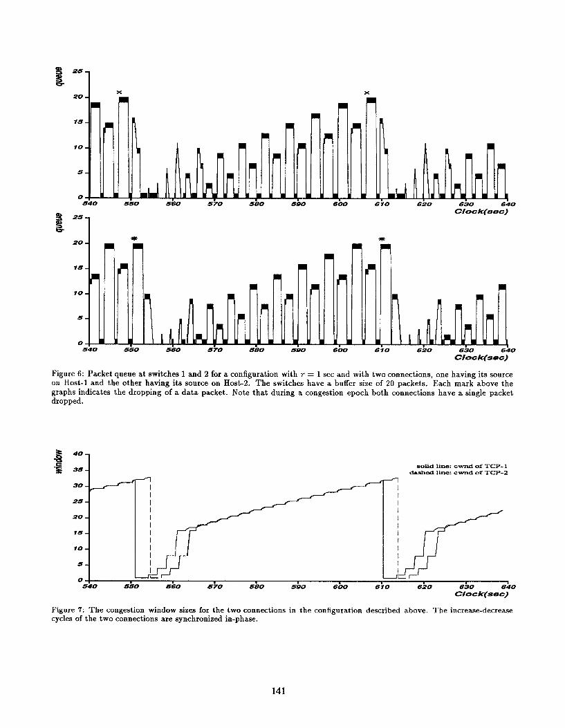
Figure 7; The congestion window sizes for the two connections in the configuration described above. The increase-decreasecycles of the two connections are synchronized in-phase.

141

60.34

so .

40.

30. 1 25

20

70

10 1 , , , I

S40 542 544 546 S48 550 5S2 664 556 5S8 560Clockf-see)

60

1so

40 11 25

20-

10-

0-540 542 544 546 54s 560 5s2 554 5s6 55B 560

cIock{sec)

Figure 8: Packet queues at switches 1 and 2 for a configuration with r = 0.01 sec. There are two connections, one having itssource on Host-1 and the other having its source on Host-2, with fixed window sizes of 30 and 25 respectively. The switches

have infinite buffers. Note that the t~o queues have different maximum heights.

3.

4.

5.

at rate RA, while the Al’s are still arriving at rate RD,

causing the length of Q2 to drop suddenly. At Q1, D1’s

are arriving at rate RA (due to the Al’s leaving Q2 atthat rate) while D1’s are leaving at rate RD, causing

the length of Q1 to increase suddenly.

Q2 has just emptied; now the Al’s that arrive at rate

RD leave at rate RD since there is no queue. At Ql,D1’s are both leaving and arriving at the same rate

RD. The queue lengths are essentially constant duringthis period. Note that all of connections 2’s packets arein Q1 (as ACK’S) during this phase, with D1’s bothahead and behind them in the queue.

The A2’s have reached the front of Q1; A2’s are leavingat rate RA and D 1‘s are arriving at rate RD, causinga sudden drop in the length of Q 1. At Q2, D2’s are

arriving at rate RA (due to the A2’s leaving Q1 atthat rate) while D2’s are leaving at rate RD, causing

a sudden increase in the length of Q2.

All of the A2’s have left Q1 and the last D2 has reachedQ2; now D1’s are leaving Q1 at rate RD and A2’s arearriving at rate RD. At Q2, Al’s are arriving at rate

RD and D2’s are leaving at rate RD. This completesthe cycle.

The explanation of the ACK-compression phenomenaused only the folIowing two assumptions: (1) ACK pack-

ets are significantly smaller than data packets, and (2) the

packets from different connections are clustered. The first

of these assumptions is almost universally valid; the sec-ond, as d~cussed in Section 3.1, is valid in th~ configu-

ration for a wide range of congestion control algorithms.Thus, we expect the phenomena of ACK-compression to

be rather common in configurations like those we have de-scribed. ACK-compression is the only effect we are aware ofwhich, in steady state, gives rise to large rapid changes inqueue lengths.

The fact that not all packets are spaced out by the trans-mission time of a data packet renders invalid our analysis in

[16] about the capacity C of the path. With two-way traf-fic, the number of packets that can be in flight at any one

time depends on how many compressed ACK’S are in thepipe. Thus, there is no longer a well defined capacity Cthat can reliably predict the occurrence of the congestionepochs. For one-way traffic, the line is fully utilized in thecongested direction (though almost completely idle in the

other direction) whenever the sum of the window sizes klarger than 2P (with data packets filling up the pipe in one

direction and ACK packets, which are spaced out by onedata packet transmission time, filling up the pipe in the

other direction). One might naively expect that with two-way traffic both lines would be fully utilized whenever thk

condition was met. This is clearly not the case. In Figure 8where P = 0.125 and the sum of the window sizes is 55,

142

25-

20.

75.

10-

s-

0 Jllwllll540 542 5M S46 S48 5s0 882 854 5S6 8S8 S60

25

4?0 -

7s -

70.

5-

Clock(sec)

0 I II 11~1 1111 11-

540 842 S44 546 548 550 552 5s4 556 8581

SfvoClock(sec)

Figure 9: Packet queue at switches 1 and 2 for a configuration with T = 1 sec and with two connections, which have sources

on- Host-1 and Host-2 and have fixed window sizes of 30 and 25, respectively. The switches have infinite buffers. Note thatthe two queues have the same maximum height, and that there is an alternation pattern in the plateau heights,

there is significant idle time when the queue for switch 2 isempty (the corresponding line has a utilization of 86%). In

Figure 9 where P = 12.5, both queues have times when theyare empty (the lines have utilization of 81 YOand 70% respec-

tively). Why does this idle time occur? We do not yet havea complete explanation, and do not have room to explain

what we do know, but the following remarks may providesome intuition. Whenever an ACK packet has to wait in

a queue, the queueing delay has the same effect as increas-ing the pipe size. Thus, even though the window sizes are

large enough to fill the actual pipes, they are not able to fillthe eflectbe pipes, Note that the size of the effective pipe

seen by a connection is a function of the window size of theother connection. Thus, increasing a connection’s window

will increase the utilization of one line, but will decrease theutilization of the other line.

We are not yet able to precisely characterize the idletime in this fixed-window system. A system which is easier

to analyze is one in which the ACK’S are of zero length. We

discuss this system again in Section 4.3.3, but make the fol-lowing observations here. As long as the pipe has nonzero

size there are no conditions in which both lines are fully uti-lized, In such a system, when the difference in window sizesis less than 2P, both lines are underutilized (as in Figure 9).When the difference is greater than 2P. onlv one line is un-

derutilized (as inReturning to

Figur~ 8).the adjustable window case, the square

wave oscillations in Figures 4 and 6 are due to the sameACK-compression phenomena just described for the fixed-window case. The only difference is that the increase in thewindow sizes in each epoch causes the plateau heights toincrease in each epoch. The observation that ACK packetsalways arrive at a queue spaced out by the data packet trans-

mission time implies that no ACK packets are ever dropped.Since a nonempty queue has decreased by at least one be-

tween every two ACK arrivals, we know that if the first ACKpacket was not dropped the second cannot be dropped ei-

ther. The first ACK packet in a cluster won’t be droppedbecause it must follow the previous data packet by at least

a data packet transmission time. This remark will be useful

in the next section, where we focus on the behavior of cwnd.

4.3 Synchronization Modes

The graphs in Figures 4-7 exhibit two different synchroniza-tion modes. When the propagation delay is small (Figures 4and 5), the connections are synchronized out-of-phase. InFigure 5, one cwnd value is rising while the other is falling.

Similarly, the two queues are out-of-phase with each other

in Figure 4. This is much like the synchronization behav-ior in the Figure 3. However, when the propagation delaysare large (Figures 6 and 7) the connections are in phasewith each other; the queue lengths rise and fall togetheras do the two cwnd values. This is much like the in-phsae

143

window-synchronization we saw in the one-way traffic cam.Simulation of other configurations reveals that typically fora fixed buffer size, the synchronization is in-phase for largeP and out-of-phase for small P. Similarly, for a fixed pipesize, the synchronization is usually in-phase for small buffersand out-of-phase for large buffers. We now discuss the out-

of-phase and in-phase synchronization behaviors separately.

4.3.1 Out-of-Phase

We first consider Figures 4 and 5 where the propagation de-

lay r of the bottleneck link is 0.01 sec. The symbols abovethe graph of the queue length in Figure 4 indicate the oc-

currence of packet drops. During each congestion epoch oneconnection loses two packets while the other connection loses

none. In the next congestion epoch, the roles are reversedand the connection which escaped without packets drops in

the previous congestion epoch now suffers the double packet

drop. Thus, in every congestion epoch the total numberof packets lost is equal to the total acceleration, but the

losses are not distributed evenly. Because one connectionloses while the other doesn’t, the window increase-decreasecycles of the two connections are synchronized out-of-phase.The current implementation of the window adjustment algo-rithm is such that, if two data packets are lost in a row, thevalue for ssthresh is reduced to its minimal value of 2.9 It

takes a long time for the connection to build its window back

up; during this time the other connection is getting most ofthe bandwidth. In fact, cwnd increases as the square root

of time over the whole cycle, rather than having an initialexponential and then linear growth periods (see [16] for a

fuller discussion of the congestion window growth iaws).The utilization of the bottleneck line is 7070 (compared

to nearly 100% for the one-way traffic case). Note that withtwo-way traffic there is considerable idle time, even herewhere the pipe is very small. This idle time is similar to

what we saw in Figure 8; since the pipe size is so small, thewindows rdways differ by more than 2P and thus only one

line is underutilized at any given time.

The presence of significant idle time remains true even ifwe increase the buffer size; when the buffer size is increased

to 60 and 120 the utilization remains at roughly 70%. Forthe various one-way configurations analyzed in [16] the frac-

tion of idle time on the bottleneck line approaches zero inthe limit of infinite buffers. This was because, as discussed

in Section 3.1, the length of a window increase-decrease cy-cle increases as one increases the buffer size, but the idletime in a cycle remains constant because it is just a func-

tion of the pipe size. This is no longer true when we havetwo-way traffic. The idle time in a cycle is a function of the

eflective pipe size which, since it is determined by the otherconnection’s window, increases with the buffer size. In fact,

the increase in the effective pipe size is proportional to the

increase in the cycle time, so that in the limit of infinitebuffers the utilization remains less than optimal.

4.3.2 In-Phase

We now turn to Figures 6 and 7 where the propagation delayr of the bottleneck link is 1 sec. Again, packet drops are in-dicated by the symbols above the graph of the queue length

‘When the first loss is detected, s.rthresh is reduced to cwnd/2,

and cw n d is reduced to 1. Upon detection of the second loss, cw n d’s

value is still 1, and ssthresh is set to its minimal allowed value which

is 2

in Figure 6. In each congestion epoch, each connection losesa single packet. Thus, even though the assumption of awell defined path capacity C which underlay the analysis in

Section 3.1 is no longer valid here, the results about eachconnection losing an acceleration’s worth of packets duringthe corr~estion eDoch seems to hold. Since the drorm are

close to each other in time, the increase-decrease cycles ofthe cwnd values and the queue lengths are all synchronizedin-phase. There are repeating periods of idle time when the

compressed ACK’s are in the pipe; the average utilizationof the line is roughly 60~0 (compared to 9070 in the one-waytraffic case with the same pipe size). Note that there are

times when both lines are idle, as in Figure 9. This is dif-ferent from the small pipe case where only one line is idle at

any moment.

4.3.3 Analysis

An obviously relevant question is: why do these two differ-

ent synchronization modes arise? Surprisingly, one can seethe root causes of these two modes in the fixed window data

in Figures 8 and 9. Consider Figure 8; in each epoch queue 1reaches a maximum of 55 while queue 2 reaches a maximumof 23. If one were to fix the buffer size to be 55 and thensuddenly increase the window sizes of both connections byone, connection 1 would suffer two losses while connection

2 would not suffer any losses. This follows from three ob-servations: (1) two packets must be dropped in order to fitin the buffer size of 55, (2) ACK packets are never dropped

(as explained in Section 4.2), and (3) packets are never lost

from queue 2 because its maximum length is well below thebuffer size. This behavior resembles the out-of-phase syn-chronization mode.

In contrast, the queues in Figure 9 both reach the samemaximal height of 23. If one were to fix the buffers sizesto be 23 and then suddenly increase both window sizes byone, both queues would overflow and thus both connections

would experience a single packet loss. This is reminiscent ofthe in-phase synchronization mode.

We are not yet able to completely characterize the dy-namics of this fixed window system. However, we do have

a conjecture for a system in which the ACK packets are of10 Let WI and ~z denote the fixed window sizeszero length ,

and assume, without loss of generality, that WI z W2. Thenlwe conjecture that there are only the following two cases.

1. WI > wz + 2P: The two queues are synchronized out-of-phase, and only one line is fully utilized.

2. WI < wz + 2P: The two queues are synchronized in-phase, and neither line is fully utilized when the in-

equality is strict.

This simple criterion completely characterizes the relevant

behavior when we have negligible size ACK’S. It appearsthat with nonzero-sized ACK’S the system continues to ex-

hibit only these two behaviors, but the simple criterion nolonger applies.

What role does the congestion control algorithm play indetermining which synchronization mode is present? Thewindow-adjustment algorithm controls the relative windowsizes during the congestion epoch; these window sizes de-termine which fixed-window case we are in. Increasing the

10Due to space limitations, we only present the content of the con-

jecture here; a fuller explanation will appear in a future publication,

144

buffers with a fixed P tends to increase the difference be-tween the window sizes at the congestion epoch, thus pro-

ducingthe out-of-phase synchronization. Increasing Pwithfixed buffers makes the criterion WI > W2+2P harder to

satisfy, thus producing the in-phase synchronization.We have simulated other configurations. Upon varying

the buffer size or the pipe size P (by adjusting the propa-gation delay r), one usually sees one of the two cases de-

scribed above. However, we have also observed behaviorwhich which does not fit neatly into our in-phase/out-of-

phase taxonomy. Usually these problematic behaviors areeither synchronized in-phase or out-of-phase, but often the

pattern of dropped packets is more complicated than we de-scribed above and violates the acceleration analysis (which

we knew was not appropriate for two-way traffic). For in-stance, there is an in-phase mode in which both connec-tions experience double drops every congestion epoch. Somemodes alternate between the single drop and double dropbehavior. Also, there is a mode in which an anomalouslylarge number (roughly 10) of packets are dropped every few

congestion epochs. We do not understand the behavior inthese other, less common, modes; they are the subject of

future work.

5 Discussion

One of the purposes of this paper is to understand the results

in [19], which we reviewed briefly in Section 3.2. Are thoseresults explained by what we have seen in our simple two-

way traffic configurations? Compare Figure 3 with Figure 4.

The rapid queue fluctuations in Figure 3 are similar to thosein Figure 4, indicating the presence of ACK-compression.Furthermore, the synchronization and idle time apparent in

Figure 3 resembles those of the out-of-phase synchronizationmode in Figure 4. These were the key features we wanted tounderstand. There are some differences, however, betweenthe data in Figure 3 and that in Figure 4; in Figure 3 the

plateaus of the square-wave-like fluctuations are narrower,the queue length rise more rapid, and the dynamics signifi-

cantly less regular.

The widths of the plateaus reflect the sizes of packet clus-

ters. Recall that the configuration analyzed in Figure 3 hada buffer of size 30, with five connections in each direction and

r = 0.01 sec. Thus, if the dynamics were completely regu-

lar and symmetric, each connection would have a maximumwnd x 6 during the congestion epoch. Thw is in contrastto the maximum wnd values of roughly 17 aud 33 (see Fig-

ures 5 and 7) for the simpler configurations considered inthis paper. This explains the narrowness of the plateaus.

The rate at which the queue size rises is related to thetotal acceleration and the total acceleration during a con-

gestion epoch is just the total number of connections. Sincewe have 10 connections in the configuration for Figure 3compared to just 2 for Figure 4, we would expect the queuelerwth to rise much more raDidlv in Fimre 3.

“The regularity in the simile ~onfigu~ations considered in

this paper is due to the complete clustering of the packets.We have explained in [16] why this clustering occurs for

one-way traffic configurations. It also holds when there isa single connection in each direction. 11 However, completeclustering does not always occur when there are multipleconnections in each direction because not all connections

11 The argument in [16] can easily be extended to include this case;

for the sake of brevity, we have omitted this argument.

lose packets during the same congestion epoch. There is stillsome degree of clustering, in that most packets are followed

in the queue by packets from the same connection, but theclustering is no longer complete nor regular. This causes the

dynamics in Figure 3 to be somewhat irregular.

We have spent considerable time focusing on the phe-nomena of ACK-compression and synchronization modes.It is natural to ask how general these results are. The pree-

ence of the two phenomena relied on two crucial properties:(1) ACK packets are significantly smaller than data pack-

ets, and (2) the packets from each connection are clusteredtogether. We therefore expect that any configuration which

satisfies these two properties will exhibit the phenomena ofACK-compression and synchronization modes. There are

two aspects of a configuration; the flow control algorithmsand the net work topology.

In thw paper we have only considered the BSD 4.3-TahoeTCP congestion control algorithm. However, we expect ourresults to be more generally applicable. Other nonpacedwindow adjustment algorithms will also have the clustering

effect, and thus we would expect to see ACK-compressionand synchronization modes for those algorithms as well.

Similarly, we have only considered one very simple net-work topology. But, once again, as long as some degree of

packet clustering exists, we expect the phenomena of ACK-compression and synchronization modes to be important as-

pects of the traffic dynamics. Therefore a crucial questionis: for what kinds of network configurations are the packets

at least partially clustered? We do not yet know the an-swer to this question. However, for a topology considered in

[19] consisting of four switches, with a traffic pattern of 50connections whose path lengths were roughly equally splitbetween 1, 2, and 3 hops, the queue length data displayed

both the ACK-compression and out-of-phase synchroniza-tion phenomena. Thus, even in thw rather complicatedtopology where a detailed analysis of the dynamics is in-feasible, the basic aspects of the behavior are due to the

phenomena we have discussed here.

On the other hand, we know at least two kinds of modifi-cations to the configuration that can reduce packet cluster-ing to some extent. First, the fact that the two connections

had the same round-trip time was crucial to the completepacket clustering in our simulation. When the round-trip

times of different connections differ by more than a packettransmission time at the bottleneck point, the clustering will

no longer be perfect, although partial clustering may still ex-ist. Secondly, the delayed-ACK option (see Section 2.1) in

the current BSD 4.3-Tahoe TCP implementation introducessome elements of pacing, not by changing what the source

does but by modifying how soon the receiver responds to ar-rived data. With the delayed-ACK option on, the receiverwill hold back the acknowledgment to an arrived data packetuntil a second data packet arrives or until a timer, whichhas a rather conservative timeout value, expires; both ofthese actions effectively delay the ACK to the first packet

by at least a packet transmission time. We have simulatedthe behavior with this option on. For small window sizes

(e.g., rnaxwnd = 8), the packets in the window are cut intoa few small partial clusters minimizing the effect of ACK-

compression. When the window sizes are large, however,some partial clusters are of appreciable size, and the effectof ACK-compression becomes significant again. Thus, thedelayed-ACK option reduces the degree of clustering, andhence the effect of ACK-compression, to some degree butdoes not eliminate it.

145

It is reasonable to ask if the phenomena we have de-scribed here are merely artifacts of our unrealistically sim-

ple simulation model. A piece of closely related work byWilder et al. ([17]), which we received after the completionof our work, describes some measurements on an 0S1 testbednetwork. The testbed configuration was somewhat similar

to those considered here, but with longer paths and variousnumbers of connections going in each direction. The hosts in

the testbed run an implementation of the 0S1 transport pro-tocol TP4 enhanced with the CE-bk congestion avoidancealgorithm ([1 5]). Even though this congestion control algo-rithm has shown fair throughput allocations in previous testswith one-way traffic configurations (on the same testbed),

the two-way traffic measurements revealed extreme unfair-

ness. This unfairness was ascribed to rapid queue lengthfluctuations caused by ACK-compression, which seriouslyinterfered with the switch’s load averaging aJgorithm. It wasalso noted that, as we have seen here, the lines were signif-

icantly underutilized. These measurements on a real net-work suggest that the phenomena we described: (1) are not

simulator artifacts, (2) exist in reaJ implementations withdifferent window-based congestion control algorithms, and(3) can have a significant and harmful effect on congestioncontrol algorithms which were designed with the assump-

tion that ACK’S would provide sufficient clocking to keepthe queue length fluctuations minimal.

6 Summary

This paper addressed the nature of network dynamics in asimple network with two-way traffic controlled by the BSD

4.3-Tahoe TCP implementation. Two-way traffic exhibitsseveral of the same phenomena that we found in one-way

traffic. The packets from each connection are clustered to-gether, and the number of losses can be roughly estimated

by the acceleration analysis. However, there are two phe-nomena that are new to two-way traffic. First, there isACK-compression caused by the interaction of ACK anddata packets in a queue. ACK-compression produces rapidand large fluctuations in the queue length. It also rendersinvalid the assumption that ACK’S provide reliable clocksfor data transmissions. In addition, ACK-compression cangive rise to significant idle time even when the flow con-

trol windows are large compared to the pipe size. Second,two-way traffic has two synchronization modes. The out-of-

phase synchronization mode has the counterintuitive prop-erty that increasing the buffer size does not always result in

higher throughput.

Even though our analysis was restricted to a very spe-

cial case, it appears that the insight gained from these simplenetworks appears to apply, at least in part, to more generaJ

situations. However, there are many unresolved issues. Thedynamics in more complicated networks is still very poorlyunderstood. Also, it is not clear what relevance our results

have for the Internet or other similar large-scale networks.

For instance, is ACK-compression a common phenomenon

in these networks? Are the packets from different connec-tions clustered in network queues, or or are they mostlyinterleaved? These questions await careful measurement.

Finally, one can ask whether what we have seen here hasany implications for the design of new congestion control

algorithms. We have seen that a standard rule-of-thumb

is not valid with t we-way traffic; ACK’s are not reliableclocks, even in steady state. Thus, future designs must find

more reliable means to supply this clocking function. Per-haps most importantly, we have also seen that minor mod-

ifications in protocol implementations can have a profoundand unintended impact on the performance. For instance,the delayed-ACK option was originally intended solely to

decrease the network overhead by reducing the number of

ACK’S. However, this slight change to the ACK’ing behav-ior can significantly alter the traffic dynamics. When seem-

ingly minor implementation changes can have unintendedand unexpected consequences, how does one separate the

implementation specific details of an algorithm from the es-sential features needed for adequate performance?

References

[1]

[2]

[3]

[4]

[5]

[6]

[7]

[8]

[9]

[10]

[11]

[12]

R. Braden (editor). Requirements for Inter-net hosts -communication layers, RFC-1122, October 1989.

J. Davin and A. Heybey. A Simulation Stw-lg of FairQueueing and Policy Enforcementj In ACM Com-

puter Communication Review, 20(4), pp. 23-29, Oc-tober, 1990.

A. Demers, S. Keshav, and S. Shenker. Anai@s and

Simulation of a Fair Queueing Algorithm, In Journalof Internetworking: Research and Experience, 1, pp.

3-26, 1990.

S. Floyd and V. Jacobson. Trafic Phase E#ects inPacket-Switched Gateways, In ACM Computer Com-munication Review, 21(2), pp. 26-42, April, 1991.

E. Haahem. Analysis of Random Drop for Gateway

Congestion Control, In Report LCS TR-465, Labora-

tory for Computer Science, Massachusetts Instituteof Technology, 1989.

V. Jacobson. Congestion Avoidance and Control. InProceedings of SIGCOMM ’88, pp. 314-329, August

1988.

V. Jacobson. Berkeley TCP evolution from i.$tahoeto i.3-reno. In Proceedings of the Eighteenth In-

ternet Engineering Task Force, Vancouver, BritishColumbia, August, 1990.

R. Jain, K. K. Ramakrishnan, and D.-M. Chiu. Conges-tion Avoidance in Computer Networks with a Connec-tionless Network Layer, In Innovations in Network-

ing, edited by Craig Partridge, Artech House, Boston,

1988.

A. Mankin and K. Thompson. Limiting Factors inthe Performance of the Slow-Start TCP Algorithms,

In Proceedings of USENIX Winter’89 Conference,1989.

A. Mankin. Random Drop Congestion Control, In F’ro-

ceedings of SIGCOMM ‘9o, pp. 1-7, September 1990.

D. Mitra and J. Seery private communication

D. Mitra and J. Seery Dynamic Adaptive Windows forHigh Speed Data Networks: Theory and Simulation In

Proceedings of SIGCOMM ‘9o, pp. 30-40, September1990.

146

[13] J. Nagle. Congestion Control in TCP\IP Internet-works, ACM Computer Communication Review,

14(4), October, 1984.

[14] J. Postel. DoD Standard Transmission Control Proto-

col Net work Information Center RF C-793, SRI Inter-

national, September 1981.

[15] K. Ramakrishnan and R. Jain A Binary Feedback

Scheme for Congestion Avoidance in Computer Net-

works ACM Transactions of Computer Systems, Vol

8, No.2, May 1990.

[16] S. Shenker, L. Zhang, and D. Clark. Some Observations

on the Dynamics of a Congestion Control Algorithm, InACM Computer Communication Review, 20(4), pp.

30-39, October, 1990.

[17] R. Wilder, K. K. Ramakrishnan, and A. Mankin Dy-namics of a Congestion Control and Avoidance of Two-Way Trajic in an OSI Testbed, In ACM Computer

Communication Review, 21(2), pp. 43-49, April, 1991.

[18] L. Zhang. A New Architecture for Packet Switching

Network Protocols, In Technical Report TR-455, Lab-oratory for Computer Science, Massachusetts Insti-

tute of Technology, 1989.

[19] L. Zhang and D. Clark. Oscillating Behavior of Net-work Trafic: A Case Study Simulation, In Journalof Internetworking: Research and Experience, 1, pp.

101-112, 1990.

147