Working Paper SeriesCongressional Budget Office

Washington, D.C.

OCCUPATIONAL EMPLOYMENT RISKAND ITS CONSEQUENCES FOR UNEMPLOYMENT DURATION AND WAGES

Ignez M. TristaoCongressional Budget Office

Washington, D.C.E-mail: ignez.tristao@cbo.gov

January 20072007-01

Working papers in this series are preliminary and are circulated to stimulate discussionand critical comment. These papers are not subject to CBO’s formal review and editingprocesses. The analysis and conclusions expressed in them are those of the authors andshould not be interpreted as those of the Congressional Budget Office. References inpublications should be cleared with the authors. Papers in this series can be obtained athttp://www.cbo.gov/publications/.

Abstract

There are substantial differences in unemployment durations and reemployment outcomesfor workers in different occupations. This paper shows thatthis variation can be explained inpart by differences in occupational employment risk that arise from two sources: (1) thediversification of occupational employment across industries, and (2) the volatility ofindustry employment fluctuations, including sectoral comovements. The analysis combinesdata from the Quarterly Census of Employment and Wages with the National LongitudinalSurvey of Youth 1979 male sample. Applying a competing risk duration model, this analysisfinds that unemployed workers in high employment risk occupations have 5.2% lower hazardratios of leaving unemployment to a job in the same occupation and have 4.9% higher wagelosses upon reemployment than workers in low employment risk occupations. Amongoccupational switchers, workers in higher employment riskoccupations have 11% higherwage losses than workers in lower employment risk occupations.

1. Introduction 1

This paper documents substantial differences in unemployment durations and

reemployment outcomes across workers in different occupations. It also argues that this

variation comes in part from the fact that some occupations have a more diversified portfolio

of employment choices than others. For instance, occupations common to many industries,

like accountants, have a well-diversified portfolio of employment opportunities, while

occupations common to only a handful of quite volatile industries, like earth drillers, have a

much more concentrated portfolio of employment options.

Looking at the data, one can observe a large variation in average unemployment

durations and wage losses across occupations (see Table 1 and Figure 1).2 A striking aspect

of these numbers is that differences in unemployment duration and wage losses are present

even among closely related occupations with seemingly similar levels of skills, education,

training, and work performed. For instance, there are largedifferences in duration and wage

outcomes both among low-skill blue-collar occupations (e.g.,between “fabricators and

assemblers” and “handlers and laborers”) and among high-skill white-collar occupations

(e.g., “engineering and science technicians” and “other technicians”). This suggests that

variation in workers’ characteristics alone, especially in educational attainment, cannot

explain why individuals in some occupations face longer unemployment spells and greater

wage losses than individuals in other closely related occupations. Figure 2 presents

1I would like to thank John Rust, Seth Sanders, John Shea, BillEvans, Mark Duggan, Jeffrey Smith, JudithHellerstein, Audrey Light, Jay Zagorsky, Steve McClaskie,Alex Whalley, and Juan Contreras for invaluablecomments and suggestions.

2These averages are reported for 45 detailed occupational codes, an intermediate occupational classification(between two- and three-digit codes), established by the Current Population Survey (CPS).

1

occupational differences in average wage change upon reemployment for occupational

stayers and occupational switchers.3 We can see from this figure that wage loss variation is

present regardless of whether workers switch occupations or not upon reemployment.4

Past studies of unemployment duration and wage determination have acknowledged the

relevance of an individual’s occupation by differentiating workers either between blue- and

white-collar occupations or by their main occupational groups. However, only recently have

studies tried to investigate why occupations are importantto employment and wages. For a

long time, economists have considered firm-specific skills to play a major role in earnings

determination.5 Conflicting findings regarding the magnitude of tenure effects on earnings

profile led Neal (1995) and later Parent (2000) to examine whether industry-specific human

capital is more important in explaining earnings than firm-accumulated skills. Both studies

find evidence in favor of industry-specific skills.

Most recently, a growing line of work has emphasized occupation rather than industry

as the level of human capital specificity that is relevant to earnings. Kambourov and

Manovskii (2002) and Poletaev and Robinson (2003 and 2004) show that the evidence for

industry-specific capital is weak and that the data are consistent with a more general skill

measure of human capital, like occupation. They find that when occupation or a set of skills

specific to an occupation is taken into account, industry andfirm-specific human capital lose

3Occupational stayers are workers reemployed in the same occupation they held in their previous job, whileoccupational switchers are those that change occupation upon reemployment.

4I also examined whether this observed variation on wage losses was due to an uneven distribution of dis-placed workers across occupations, since they may suffer greater wage losses upon reemployment than non-displaced workers. However, even for displaced workers I still find the same large variation, whether or not theyswitched occupations upon reemployment. Displaced workers are those that report losing their jobs due to layoffor plant closing.

5See Abraham and Faber (1987), Altonji and Shakotko (1987), and Topel (1991). For a complete discussionof the literature see Willis (1986).

2

their importance in explaining earnings. Their results suggest occupation captures an

important component of human capital that is relevant for earnings determination.6 Thus

unemployed workers have an incentive to look for a job in the occupation they held

previously so that they can retain and therefore capitalizeon their occupation-specific human

capital.

Another aspect of human capital that has attracted attention in recent years is the labor

income risk associated with different skills. It has becomecommon in the literature to

assume that individuals with different skills or levels of accumulated human capital face

different labor income risk.7 In this paper, however, I show that there is another aspect of

human capital risk that has not been studied and that seems tohave an important role in

explaining observable differences in unemployment duration and wage losses across

occupations. In particular, I analyze differences in the diversification of employment

opportunities faced by each occupation. I argue that differences in this risk arise from the

large variation in the distribution of occupational employment across industries and from the

fact that industries have different employment volatilities.

The combination of these two facts implies that some occupations have a more

diversified portfolio of employment opportunities than others. This suggests that individuals

employed in more diversified occupations potentially face lower unemployment risk than

those in occupations with lower diversification, and may thus experience shorter

6Occupations are, in general, classified based on an exclusive set of specific skills and skill demands thatuniquely define them. Among this set of specific skills are thenature of work performed, education, training, andwork credentials.

7Most studies measure human capital risk as differences in the variance of labor income associated withdifferent levels of skills. See, for example, Grossmann (2005) and Huggett, Yaron, and Ventura (2005).

3

unemployment spells and/or lower wage losses upon reemployment. I call this phenomenon

occupational employment risk (OER).

Regarding the distribution of occupational employment, occupations can differ both in

the number of different industries that employ them8 and in their concentration across these

industries. Looking at the data, one can see that there is a quite large variation in the number

of industries that employ different occupations (see column 1, Table 2). For instance, in the

1990 Census data “accountants” are employed by 157 out of 158three-digit industries, while

“earth drillers” are employed by only 13 of these industries(see Figure 3).9

In addition, occupations vary enormously in the concentration of their employment

across industries. It is not uncommon to see occupations with more than 75% of their

employment concentrated in one or two industries, regardless of how many industries employ

the occupation. These differences in occupational employment concentration across

industries can be well summarized by a Herfindahl index of employment concentration.10

Table 2 presents the Herfindahl index for each occupation. Similar to unemployment duration

and wage loss, there is large variation in the concentrationof occupational employment

across industries. Some occupations, like “handlers and laborers” and those in “financial

records”, have very low Herfindahl values and therefore low industry employment

concentration, while occupations like “teachers” and “construction laborers” are highly

concentrated in a few industries. Figure 4 graphs the Herfindahl values for all occupations

8In a sense this captures how transferable occupational skills are across industries.9Appendix A.2 provides details on occupational and industrycodes.

10A Herfindahl index of employment concentration can be obtained for each occupation by summing, acrossall industries, the squared shares of the occupation’s employment in each industry. This index is bounded between0 and 1; the higher its value, the more concentrated across industries the occupational employment.

4

shown in Table 2. Even within major occupational groups, there is large variation in the

concentration of occupational employment (see, for example, the difference between

“teachers” and “engineers”).

Aside from differences in the distribution of occupationalemployment, variation in

industries’ employment fluctuations is also important to occupational employment

opportunities and should be taken into account when studying occupational employment risk.

Given the uneven distribution of occupational employment across industries, differences in

industries’ employment fluctuations11 can greatly affect the portfolio of employment

opportunities faced by each occupation. Returning to the case illustrated by Figure 3, both

“accountants” and “earth drillers” are employed by the construction industry, which is highly

volatile. We can see from the figure that more than 80% of “earth drillers” are employed by

the construction sector and that only a few other industriesemploy them. Among those are

“metal mining”, “nonmetal mining”, and “cement, concrete,and plaster products”, all of

which are very volatile and exhibit strong temporal comovement with construction. So if the

construction sector is hit by an idiosyncratic shock and lays off many workers, including

“earth drillers” and “accountants”, “earth drillers” would probably have a harder time finding

a new job in the same occupation, since the construction industry is their main employer, and

the other industries that employ them are probably comovingwith construction (being

affected by the same shock). Unemployed earth drillers can change occupation in order to

shorten their unemployment spell; however, we know from Kambourov and Manovskii

(2002) and Poletaev and Robinson (2003 and 2004) that if theydo so they are likely to have a

11Some industries face more frequent and/or larger shocks than others. For example, low aggregate demandor high oil prices can affect some industries more heavily than others. Sectors like construction, transportation,and services, for instance, are usually more volatile than other sectors.

5

higher wage loss, since they lose their occupation-specifichuman capital. Accountants,

however, can more easily leave the construction sector and look for an accountant job in a

different industry. In fact, only 5.2% of accountants are employed in construction and they

can work for any other industry in the economy, many of which will not be comoving with

construction.

In this paper, I combine the specific- human capital preservation motive with

employment risk variation to explain differences in unemployment duration and wage losses

across occupations. In order to do so, I define a measure of occupational employment risk,

which I estimate using data from the Quarterly Census of Employment and Wages, years

1979-2000. I then relate this measure to unemployment duration and wage loss using a

constructed weekly panel of employment and demographic histories for 5,579 males in the

National Longitudinal Survey of Youth 1979 (NLSY79), whichincludes employer

characteristics for up to five jobs each individual held during any year in the period

1979-2000. I find, as expected, that workers in high-risk occupations, as defined by the OER

measure, have lower hazard ratios of leaving unemployment to a job in the same occupation

and have higher wage losses than workers in low-risk OER occupations, especially if they

switch occupations.

The paper is divided into five sections. Section 2 discusses the methodology used in

order to measure occupation employment risk. Section 3 estimates the effect of OER on

unemployment duration, while Section 4 relates this risk measure to wage losses. Section 5

presents conclusions and suggestions for future work.

6

2. Measuring Occupational Employment Risk (OER)

In this section, I define and construct a measure that dependsboth on the diversification

of occupational employment across industries and on the level of industry employment

volatility, including comovements. The employment opportunities of an occupation can be

seen as a portfolio of industries where the weights are the shares of occupational employment

in each industry and the rates of return are the industry volatilities.

To my knowledge, this study is the first to define and calculatea measure of

employment risk associated with particular occupations, although a number of studies have

estimated either the risk associated with aggregate employment volatility or different

industries’ unemployment risk. Neumann and Topel (1991) measure unemployment risk for

workers in a particular locality as the variance of the within-market local demand uncertainty,

e′V, wheree is the vector of local industry employment shares andV the vector of estimated

sectoral local employment shocks. Based on the assumption that workers are mobile within

local markets,12 they show that the sectoral composition of the market forms an implicit

“portfolio of employment opportunities in which less specialized markets may achieve lower

unemployment.” The authors find that their measure explainsdifferences in unemployment

rates among geographically distinct labor markets.13 Through the use of a similar measure,

Shea (2002) finds that interindustry comovement is responsible for 95% of the variance of

manufacturing employment.14 Using 126 three-digit U.S. manufacturing industries over the

12Their argument is based on the assumption that if there are many goods and if skills are transferable, workersare mobile within local markets.

13In addition, they show that within-market changes in demanduncertainty had positive but only minor effectson within-market changes in unemployment.

14Shea estimates that the average pairwise correlation of annual employment growth is 0.34 and that, evenafter aggregating industries to 20 two-digit industry codes, comovement is still responsible for over 86% of

7

period 1959-1986, he estimates aggregate employment risk by decomposing annual

employment growth into an average of industry growth rates,weighted by the industries’

share of employment.

My idea builds on the fact that occupational employment is distributed unevenly across

industries: some occupations are employed in many industries, while others are employed in

only a small number of industries. Furthermore, different industries have different

cyclicalities. In this context, it is reasonable to expect that different occupations may have

diverse levels of employment risk associated with them. Occupations common to a larger

number of industries may face a lower employment risk given that they have more diversified

employment opportunities. In order to examine whether thisis really the case, I construct a

measure of occupational employment risk (OER) that considers two important dimensions of

risk: the concentration of occupational employment acrossindustries and the volatility and

comovement of disaggregated industry employment. The OER measure is calculated in a

fashion similar to the calculations of Neumann/Topel and Shea.

The concentration component of the OER measure is obtained by calculating the shares

of occupational employment in each industry.Sv j is the share of occupationv in industry j,

defined as follows:

Sv j =empv j

empv, (1)

whereempv j is the employment of occupationv in industry j andempv is the total

employment in occupationv. I assume the shares to be in steady-state and compute them

manufacturing employment variation. For more on comovements, see Long and Plosser (1983) and Horvath(1998).

8

from the 1990 Census Public Use Microdata Series (PUMS) by constructing an

occupation-by-industry employment matrix. I must make a steady-state assumption due to

the lack of annual data on occupational employment by industry for the time period I

consider. The limitation of making such an assumption is that if the occupational

employment shares change significantly over time, my measure of OER will not capture

these trends.15 However, given that I am using a more aggregated occupational classification,

these shares should be more robust to changes over time. Nevertheless, as a robustness check,

I also estimated a version of OER using 1980 Census shares andobtained similar results.16 I

use 1990 shares since 1990 is the midpoint of my analysis.

The volatility component,Ωε, is constructed using the variance-covariance matrix of

disaggregated industry employment growth rates,ε jt , j = 1, ...J, andt = 1978, ...2000, which

I estimate using data from the Quarterly Census of Employment and Wages (QCEW) over

the period 1978 to 2000.17 In particular, note thatΩε incorporates not only the variance of

industry employment but also comovements among industries.18 The QCEW contains

information on the number of establishments, employment, and total wages of employees

covered by various unemployment insurance programs. A nicefeature of this data set is that

it provides industry employment data for every four-digit industry at national, state,

15Note that the steady-state assumption of the shares of occupational employment in each industry is consis-tent with the well-known phenomenon of skill upgrading within industries, as long as all industries are sheddingless-skilled workers at the same rate.

16The overall correlation of the shares of occupational employment in each industry between 1980 and 1990is 0.98. Calculating this correlation separately for each occupation, I find the lowest correlation to be quite high(0.79 for “personal services occupations”).

17Specifically,ε jt =∆log(empjt ).18I have tried different specifications for estimatingΩε. In particular, using industry employment shocks

estimated by controlling for industry-specific characteristics with and without year dummies, I obtain similarresults, regardless of the specification I use, so I opted forthe simplest specification.

9

metropolitan statistical area (MSA), and county levels forthe period 1975-2004.19 The main

limitation, however, is the change in industry codes over the time period (years 1975-1987

use the 1972 SIC, 1988-2000 use the 1987 SIC, and 1990-2004 use the NAICS). I deal with

this issue by matching industry codes between the first two time periods in order to make the

industry classification consistent for 1978-2000. The criterion I used was to merge 3-digit

industry codes if one or more of their 4-digit industries arereported to be combined. Details

about the industry code matching are in the appendix.20

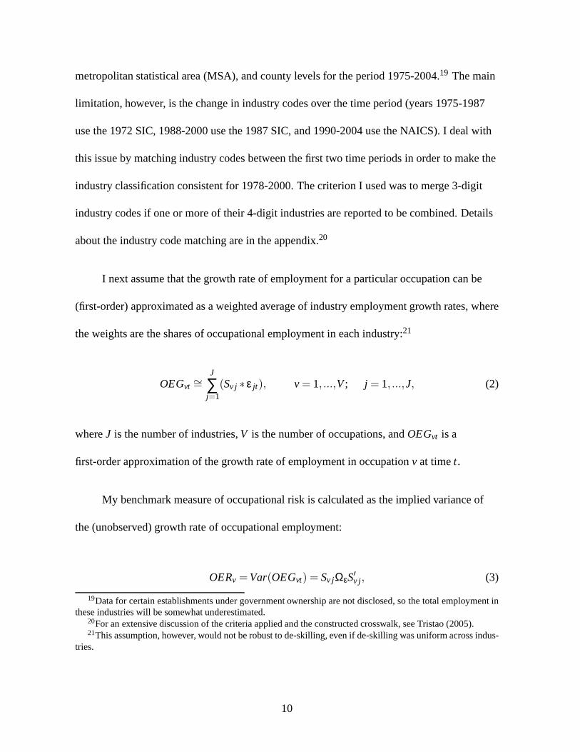
I next assume that the growth rate of employment for a particular occupation can be

(first-order) approximated as a weighted average of industry employment growth rates, where

the weights are the shares of occupational employment in each industry:21

OEGvt∼=

J

∑j=1

(Sv j ∗ ε jt ), v = 1, ...,V; j = 1, ...,J, (2)

whereJ is the number of industries,V is the number of occupations, andOEGvt is a

first-order approximation of the growth rate of employment in occupationv at timet.

My benchmark measure of occupational risk is calculated as the implied variance of

the (unobserved) growth rate of occupational employment:

OERv = Var(OEGvt) = Sv jΩεS′v j, (3)

19Data for certain establishments under government ownership are not disclosed, so the total employment inthese industries will be somewhat underestimated.

20For an extensive discussion of the criteria applied and the constructed crosswalk, see Tristao (2005).21This assumption, however, would not be robust to de-skilling, even if de-skilling was uniform across indus-

tries.

10

whereSv j is a 1×J vector of occupationv′s industry shares andΩε is aJ×J matrix of

variances and covariances ofj ′s employment growth rates. It is worth noting that this

measure has a lower bound at zero but is unbounded from above.

The OER measure is estimated for 158 3-digit industry codes and 45 “detailed”

occupational codes, an intermediate occupational classification (between two- and three-digit

codes), given by the Current Population Survey (CPS).22 There are two main advantages to

using this classification of occupations. The first is that workers may consider their skills to

fit more than one three-digit occupation, which could lead them to search for a job in a

closely related occupation. For example, a worker whose three-digit occupation is “payroll

and timekeeping clerk” may also apply for “billing Clerk” jobs.23 Second, a more aggregate

classification reduces the problem of measurement errors from occupational

misclassifications, which is an issue in other longitudinalstudies using occupations.24

Nevertheless, the CPS detailed occupational codes is stillquite a rich classification, with

three times as many occupational categories as the two-digit code.

Figure 5 presents the OER measure for different occupations. One can see that there is

a large variation in this measure of employment risk across occupations, even within closely

related occupational groups. In the next two sections, I relate this measure to unemployment

duration and wage loss in order to examine whether workers inhigher employment risk

occupations indeed face longer unemployment spells and wage losses than workers in lower

22See Appendix A.2 for a description.23These two occupations are classified as being closely related by the Occupational Outlook Handbook pub-

lished by the Bureau of Labor Statistics (BLS).24See Kambourov and Manovskii (2002 and 2005) and Neal (1995) for discussions.

11

employment risk occupations.25

3. OER Measure and Unemployment Duration

In this section, I estimate the effect of OER on the hazard rate of leaving unemployment

and, consequently, on the length of unemployment spells. Inlight of recent evidence showing

the relevance of occupation-specific human capital to earnings, unemployed workers have an

incentive to look for a job in the occupation they held previously, so they can retain and

therefore capitalize on their occupation-specific human capital. This suggests that it is

important to distinguish between two exit modes from unemployment: finding a job either in

the same or in a different occupation. In order to take these two exits into account, I use a

continuous-time competing risk model, which I estimate by using a Cox proportional hazards

model with multiple spells and time-varying covariates.26 It is worth noticing that this

procedure also takes into account the order in which these unemployment spells occur.

The main reason for choosing this specific regression model is that it allows me to

estimate the relationship between the hazard rate and explanatory variables without imposing

any parametric assumption about the shape of the baseline hazard function,h0(t).27 Not

having to parameterizeh0(t) is desirable in this context because it eliminates the need to

make assumptions on how the hazard changes over time. Incorrect assumptions on the shape

of h0(t) would produce incorrect results regarding how the covariates affect the hazard. The

25The correlations between the OER measure and the average unemployment duration and wage loss are 0.18and−0.16, respectively.

26See Jenkins (2004), chapter 8.27Cox (1972) proposes a method for estimating the covariates without having to make any assumptions about

the shape of the baseline hazard function, which in fact is not even estimated. This method relies on the assump-tion of proportional hazard and is estimated by partial likelihood rather than maximum likelihood.

12

only assumption made concerning the shape ofh0(t) is that it is the same for everyone.28 The

Cox model is often called semiparametric because the effectof the covariates is

parameterized and is assumed to shift the baseline hazard function multiplicatively. The

hazard rate for theith subject in the data is:

h(t/xi(t)) = h0(t)e(xi(t)βx), (4)

The baseline hazard can be estimated separately, conditional on the estimates ofβx. I specify

the relative hazard to be:

e(xi(t)βx) = exp(β1OERv +βxXi(t)+βzZi(t)) (5)

whereOERv is the occupational employment risk measure for occupationv. Xit is a vector of

demographic characteristics that include age, measures ofability, a dummy for race, marital

status, and educational attainment. The measures of ability are the first two principal

components of the age-adjusted Armed Services Vocational Aptitude Battery (ASVAB)

scores,29 obtained by following the two-step methodology presented by Cawley et al. (1995)

and Kermit et al. (2005). The appendix provides details.Zi(t) is a vector containing relevant

work history information, including years of work experience and tenure in the previous job,

a dummy for receiving unemployment compensation during theunemployment spell, and the

local unemployment rate.30

28See Kalbfleisch and Prentice (2002) for a rigorous treatmentand Cleves et al. (2004) for an intuitive discus-sion.

29The ASVAB is a set of ten tests measuring knowledge and skill in different areas.30In order to capture nonlinear effects, I also include quadratic terms for age, ability, experience, and tenure.

13

3.1 Construction of the Panel

The data set I use to assess the relevance of the OER measure for unemployment

duration and wages is the National Longitudinal Survey of Youth 1979 (NLSY79). The

NLSY79 is a nationally representative sample of 12,686 young men and women who were

14-22 years old when they were first surveyed in 1979. Detailed information on these

individuals’ demographic characteristics and labor forceparticipation has been collected

since 1979.31 This paper uses the unbalanced panel of civilian males, covering 1979-2000,

which contains 5,579 individuals.32

I restrict the sample to individuals who were at least 21 years old at the beginning of an

unemployment spell. In order to exclude possibly discouraged workers, in the unemployment

duration analysis, I further restrict the sample to unemployment spells whose duration were

less than 53 weeks. Furthermore, I consider only “completed” spells, which I define as a

transition from employment to unemployment and then back toemployment again, except

for the last spell in the sample, which may be censored.33 The duration of a spell is the

difference in weeks between the beginning and the end of the spell.

Relative to other micro data sets, the NLSY79 has two distinct features that make it the

best data to answer my particular question. First, the NLSY79 work history data are available

on a weekly basis. Since a significant number of unemploymentspells are very short, this

high frequency is quite important.

31Data were collected annually from 1979 to 1993, and biennially from 1994 to the present.32I restrict the sample to males in order to avoid labor force participation issues that arise when including

women in the sample.33A worker is considered unemployed by the NLSY if he or she did not work at all during the survey week

and is currently searching or has searched for a job in the four weeks prior to the survey.

14

Second, and most importantly, the NLSY79 is one of few data sets that provides a

complete work history for a specific cohort, which allows researchers to analyze completed

unemployment spells.34 This is one of the most desirable attributes of a data set for studying

labor force transitions and unemployment duration, and it constitutes a significant advantage

of the NLSY79 over the Current Population Survey (CPS) data,where unemployment spells

are incomplete and cohorts change over time. Most studies analyzing unemployment

duration in the United States use CPS data on spells in progress. Based on the steady-state

assumption that flows in and out of unemployment are constantover time, existing studies

estimate either the expected length of spell duration for a synthetic cohort of individuals

entering unemployment (using continuation rates) or the average completed spell length for

the currently unemployed workers (by “doubling” the average duration of their spells).35

However, when steady-state conditions do not hold, both estimators can be biased. Rising

unemployment will cause the steady-state method to underestimate completed spell lengths,

while decreasing unemployment will cause this method to overestimate the length of spells.36

In addition to the advantages mentioned above, the NLSY79 also has ability measures and

has lower attrition rates than other longitudinal data sets(such as the Panel Study of Income

Dynamics, or PSID). The downside of using the NLSY79 insteadof the CPS is that I am able

to analyze only individuals of a specific cohort that is stillrelatively young—in 2000, the

individuals’ age range was 35 to 43 years old.

34It is possible for the NLSY to construct a complete work history for each respondent, regardless of periodof noninterview, because its survey questions are designedto recover the start and end dates for each labor forcestatus change since the date of the last interview. See Appendix A.1 for details.

35For some of the most recent and influential papers using the CPS data see Darby et al. (1997), Baker (1992),Shimer and Abraham (2002), and Shimer (2005). Some exceptions are Dynarski and Sheffrin (1986 and 1990)using the PSID.

36For studies discussing the technical difficulties in measuring completed spells see Sider (1985) and Kieferet al. (1985).

15

The NLSY79 collects detailed information on new and previously reported employers

for whom a respondent has worked since the date of last interview. For every survey year, it

reports up to five employers.37 Using start and end dates of employment, as well as the job

number assigned to each employer in every survey round (which can vary across rounds), I

linked all employers across survey years as well as to the weekly work history files.38 This

allowed me to merge employer and job characteristics, such as industry and occupational

codes, with the work history file. I also merge employees’ main demographic characteristics,

creating a weekly panel of employment and demographic histories for up to five jobs each

individual held during any year in the period 1979-2000. Forindividuals with more than one

job at a time, I consider the primary (CPS) employer as their main job. This panel allows me

to obtain good measures of work experience and tenure with a given employer, which I

calculate weekly by accumulating the number of weeks reported both working and working

for a particular employer, respectively.

Issues that normally arise with the use of occupational codes (and to a lesser extent

industry codes) are (i) individuals doing the same job can becoded as having different

occupations and (ii) the same individual working in the sameoccupation can be coded

differently across survey rounds, generating spurious occupational mobility. As I mentioned

in the last section, in order to minimize measurement errorsfrom misclassifications of

occupational descriptions, I use a more aggregated occupational classification, which

37In fact, the NLSY79 collects information for all employers for whom a respondent has worked since thedate of last interview. According to the NLSY documentationfiles, however, the number of respondents whoreport more than five jobs in each survey is less than 1% of those interviewed.

38Since employers can receive different job numbers across years, it is necessary to use beginning and endingdates as well as a series of other supporting variables that jointly taken indicate for every current survey employerthe job number it received in the previous survey and whetherit is a new job.

16

combines closely related occupations but still contains three times as many occupational

categories as the two-digit code. Taking advantage of my panel of individual work histories

within each employer, I eliminate the second type of problemby defining the occupation in

each job to be the modal value of occupational codes ever reported for that employer, instead

of the code reported in every survey round for that job. This is a significant improvement

over previous studies that have used reported occupation codes in the NLSY79,39 provided

that one accepts the assumption that there is no genuine occupational change for individuals

working for a given employer. A similar procedure was applied to industry codes.40

Table 3 shows the basic characteristics of the sample. The last two columns present the

statistics conditional on remaining in the same occupationand switching occupation upon

reemployment, respectively.41 One can see from this table that around 44% of completed

unemployment spells end in occupational mobility and that alarger fraction of workers who

remained in the same occupation are white, single, have moreexperience and tenure, and

report having used unemployment insurance. In comparison to workers who remained in the

same occupation, more occupational switchers have a college degree and report having been

displaced.42

39Neal (1999) assumes each employer’s industry and occupational codes to be the first ever reported.40For the NLSY79 civilian male sample, I estimate a significantamount of within-employer 3-digit occupa-

tion and industry miscoding over time. In fact, 88.9% of within-employer 3-digit occupational code changes and88.4% of within-employer 3-digit industry changes are spurious, transitory changes. Genuine within-employerchanges represent, respectively, only 6.66% and 7.92% of true occupational and industry mobility at the 3-digitlevel.

41Spells for which no occupational code was reported either for the previous job or the new job, or both, areomitted.

42Displaced workers are those that report losing their job dueto layoff or plant closing.

17

3.2 Results

Table 4 shows the estimated hazard ratios of the competing risk model, obtained by

estimating a Cox PH model. The coefficients can be read as the ratio of the hazards of

leaving unemployment implied by a one-unit change in the corresponding covariate. The

proportionate change is obtained by subtracting one from the estimated hazard ratios

provided in the Table.43 One can see that, indeed, the measure of occupation employment risk

seems to affect the hazard of leaving unemployment. In particular, a one-unit increase in the

OER measure reduces the hazard of leaving unemployment to a job in the same occupation

by more than 25%. In terms of standard deviations, an increase of one standard deviation in

OER reduces the hazard of finding a job by 5.2% in each week of unemployment.44

Therefore, all else equal, workers in occupations with a less diversified portfolio of

employment opportunities (higher OER) face indeed longer unemployment spells than

workers in occupations with more employment options (lowerOER). With respect to leaving

unemployment for a job in a different occupation, however, OER seems to have no effect.

Turning to other covariates, I find that being white increases the hazard of leaving

unemployment for a job in the same occupation by 44.6%, but has no effect on leaving

unemployment for a job in a different occupation. In comparison with high school dropouts,

workers with a college degree have a 56.6% lower hazard rate of getting a job in the same

occupation. An extra year of experience and tenure increases the hazard of leaving

unemployment for a job in the same occupation by 14.7% and 23.1%, respectively. An

43Notice that the benchmark coefficient is one rather than zerosince the hazard rate is the exponentiatedcoefficient.

44The mean and standard deviation values of OER are 0.06 and 0.20, respectively.

18

additional year of experience increases the hazard of getting a job in a different occupation

by 6.1%, while an additional year of tenure reduces it by 17.7%. Having received

unemployment insurance increases by 22.8% the hazard of leaving unemployment for a job

in the same occupation, while it decreases by 27.3% the hazard of getting a job in a different

occupation. A one percentage point increase in the local unemployment rate seems to have

no effect on finding a job in the same occupation but reduces by2.7% the hazard of finding a

job in a different occupation.

4. OER Measure and Wage Change

In order to assess whether OER has any effect on earnings losses when controlling for

other covariates, I examine its impact on the change in log wage between pre- and

post-unemployment jobs. In particular, I estimate an Ordinary Least Squares regression,

where unemployment spells are the unit of observation. Since the sample includes multiple

spells per individual, I use clustered standard errors to account for the additional correlation.

I estimate the following equation:

∆lnw = β0+β1OER+β2X +β3Z+β4slength+ ε, (6)

whereX andZ are the same matrices of covariates used to estimate the effects of OER on the

hazard rate of leaving unemployment, except for the unemployment rate and insurance

compensation variables. All these covariates refer to pre-unemployment values. Total weeks

of unemployment are represented byslength, which I expect to have a negative estimated

19

coefficient, given that workers tend to lower their reservation wage as the length of their

unemployment increases. In this context, when explicitly accounting forslengthin the

regression, its coefficient measures the effect of OER on wage changes through increases in

unemployment duration and lower reservation wages while the OER coefficient measures its

direct effect on wage gain or loss upon reemployment. In order to assess the total effect of

OER on wage, I also run the regressions without spell length.

I examined the effect of OER on earnings losses for three different samples: occupation

stayers, occupational switchers, and the full sample. I expect it to increase wage losses,

especially for occupational switchers. The results are shown in Table 5. In fact, we can see

that an increase in the OER measure increases the wage loss for all three samples. However,

this effect is statistically significant only for occupational switchers (with and without spell

length). In particular, a one-unit increase in the OER measure increases the hourly wage loss

by 4.88% for all workers and by 11.5% for occupational switchers. For a one standard

deviation increase in OER, the corresponding numbers are 1%and 2.3%, respectively. In

addition, longer unemployment spells translate into higher wage losses, with each extra week

of unemployment increasing the hourly wage loss by 0.1% for the full sample and by 0.2%

for occupational stayers.45 Similarly, an extra year of tenure increases wage loss by 2.1% for

the full sample and by 6.2% for occupational switchers.

These results, combined with those for unemployment duration, suggest that workers in

high-risk occupations, as defined by the OER measure, have anincentive to remain in the

45Thus high OER occupations face a 4.88% wage loss plus 0.1% forevery extra week of unemployment,while workers in high OER occupations that switched occupations had an 11.5% wage loss of plus 0.2% forevery extra week of unemployment.

20

same occupation in order to avoid incurring higher wage losses, even if this means facing

longer unemployment spells.

5. Conclusions

This paper shows an aspect of human capital risk that seems toplay an important role

in explaining observable differences in unemployment duration and wage losses across

occupations. I argue that this risk arises from large differences in the distribution of

occupational employment across industries and from the fact that industries have different

employment volatilities. These two facts imply that some occupations have a more diversified

portfolio of employment opportunities, suggesting that individuals in these occupations

potentially face lower unemployment risk than those in occupations with less diversification.

Using data from the decennial Census and the Quarterly Census of Employment and

Wages, I estimate a measure of occupational employment risk(OER). I find a large variation

in this risk across occupations. I then relate the OER measure to occupational unemployment

durations and wage losses upon reemployment, using data from the NLSY79. Applying a

competing risk duration model, I find that workers in high-risk occupations, as defined by the

OER measure, have lower hazard ratios of leaving unemployment for a job in the same

occupation and have higher wage losses than workers in low-OER occupations, especially if

they switch occupations.

A next step in this research would be to investigate whether workers receive

compensating wage differentials for this type of risk and how this risk relates to employment

21

duration as well as to the incidence of unemployment. Preliminary exploration of this issue

indicates that workers in high-OER occupations receive compensating differentials and have

longer employment spells than workers in low-OER occupations. In particular, it would be

interesting to estimate a multiple-state transition modelwith three possible labor market

states—employment, unemployment, and out-of-the labor force—and examine the effects of

the OER measure on the probabilities of exiting and enteringthese states. As in

Martinez-Granado (2002), we could allow for unobservable individual heterogeneity,

duration dependence, lagged duration dependence and statedependence. Another possibility

would be to write a Mortensen-Pissarides model with the OER measure, which would

sugesst that high-OER jobs should be more durable and have more flexible wages than

low-OER jobs.

The type of risk documented and analyzed in this paper may affect the occupational

and career choices of individuals, the search strategy of unemployed workers, and individual

decisions about consumption and precautionary savings. With respect to career choice, we

could ask if individuals take into account the risk associated with specific occupations when

they make career choice decisions. With respect to the search strategy of unemployed

individuals, it is worth noting that OER is closely related to the tradeoff between accepting a

job today or waiting for a better offer tomorrow. As shown in this paper, the risk associated

with specific occupations affects, on one hand, the wage thatindividuals receive upon

reemployment and, on the other hand, the time they have to wait to receive an offer. It

follows, then, that occupational employment risk may implydifferent outcomes in the

optimal search of unemployed individuals.

22

Finally, it would be interesting to study whether OER affects precautionary savings

and, if so, its implications for wealth holdings and consumption behavior. In the context of a

life cycle model, the type of risk implied by occupational employment diversification can

affect the employment transition matrix, which would affect optimal asset holdings. The

relevant question would be to quantify this effect either with a realistic life cycle model or

with some other empirical strategy.

23

Appendix

A.1 Weekly Labor Status

The NLSY79 Work History Data provide week-by-week records of the respondents

labor force status from January 1, 1978, through the currentsurvey date. At each year’s

survey, information is collected on jobs held and periods ofnot working since the date of the

last interview.46 Since the NLSY questions are constructed to collect a complete history for

each respondent, regardless of period of noninterview, it is possible to construct for each

respondent a continuous, week-by-week labor force status record.47 In particular, the

respondents’ labor force history is constructed by filling in the weeks between the reported

beginning and end dates for different activities (or “inactivities”) with the appropriate labor

status code.

One of the reported issues with the weekly labor status series is the presence of “split

gaps” during unemployment, when individuals are unemployed for part of the gap and out of

the labor force for the other part of it.48 Since “split gaps” are coded such that the

unemployment spell falls between two out-of-labor force spells, they are not considered to be

completed unemployment spells and are therefore not included in the sample.

46A job held any day of a week is counted as a job for the whole week.47For example, a respondent last interviewed in 1987, and not interviewed again until 1990, will have a

complete labor force history, as information for the intervening period will be recovered in the 1990 interview.The NLSY “Work Experience” section reports that although there may be potential inconsistencies generated bythis method, it does not compromise the quality and/or completeness of the work history record. For details, seeAppendix 18 of the NLSY Documentation Files.

48Although the start and stop dates for the whole gap will be those actually reported by the respondent,the assignment of the unemployed and out-of-labor-force states will not represent actual dates reported by therespondent. Instead, they represent only the number of weeks that a respondent reported having held each status,with the unemployed status being arbitrarily assigned to the middle portion of the gap. For further details on“split gaps,” see Appendix 18 in the NLSY documentation.

24

The NLSY weekly labor status variable,wk, can assume the following values:

wk=

0, cannot account for week due to invalid start and end dates;

2, cannot determine whether unemployed or out-of-the labor force;

3, employed but cannot account for all of the time with employer;

4, unemployed;

5, out of the labor force;

7, active military service;

> 7, employed.

For about 1% of the weeks in the male, nonmilitary samplewk is equal to 0. When

employed, the assigned code is the actual survey number multiplied by 100 plus the job

number for that employer in that year. Based on this classification, I generated a weekly

employment status that assumes the following values:49

empstat=

employed if wk = 3 or>7

unemployed if wk = 4 or (wkt=2)&(2 ≤wkt−1 ≤4) or (wkt=2)&(wkt−1>7)

other if empstat6= 1 or 2

A.2 Industry and Occupational Codes

The Census defines an industry as a group of establishments that produce similar

products or provide similar services. Although many industries are closely related, each has a

unique combination of inputs and outputs, production techniques, occupations, and business

49It is worth noting that I do not include individuals who ever worked in the military.

25

characteristics. Occupations are classified based on work performed, skills, education,

training, and credentials. The classification system covers all occupations in which work is

performed for pay or profit and is intended to classify workers at the most detailed level

possible.

The universe used by the Census for occupation and industry variables comprises

individuals age sixteen or older who worked within the previous five years and are not

considered new workers.50 Occupation and industry codes report the person’s primary

occupation and industry, which are considered to be the onesin which the person earns the

most money; however, for respondents unsure about their income, their primary occupation

and industry were considered those at which they spent the most time. If a person listed more

than one occupation and/or industry, the samples use the first one listed. The occupational

codes were assigned based on the following two questions: (1) What kind of work was this

person doing? and (2) What were this person’s most importantactivities or duties? The

industry codes were assigned based on the following three questions: (1) For whom did this

person work (name of company, business, organization, or other employer)? (2) What kind of

business or industry was this? and (3) Is it mainly manufacturing, wholesale trade, retail

trade, or other?

Matching Industry Codes

In order to estimate the OER measure, I calculate the concentration of occupational

employment across industries and the volatility and comovement of disaggregated industry

50“New workers” are defined as persons seeking employment for the first time who have not yet secured theirfirst job.

26

employment. Given the fact that there is no single data set with occupational employment by

industry during the period of analysis (1979-2000), I combine data from two different

sources to compute both components of the OER measure.

I use data from the 1990 Census to calculate the concentration component of the OER

measure, which is obtained by calculating the shares of occupational employment in each

industry. The volatility component was estimated using data from the Quarterly Census of

Employment and Wages (QCEW), 1978-2000. However, these twodata sources use different

industry classification systems. The Census uses the CensusIndustrial Classification (which I

will call CIC), while the QCEW uses the Standard Industrial Classification (SIC) System. In

order to estimate OER from these two data sets, I need to matchthe industry codes across the

industry classification systems. In addition, both classification systems experience changes

over time. Therefore, it is necessary to match industry codes across classification systems

and over time in order to have consistent industry codes overthe period of analysis. An

extensive discussion of all criteria applied in this matching is given in Tristao (2005). I

choose the 1980 Census industry and occupational codes as the base codes for this study. I

discuss the occupational codes’ matching in the next subsection.

Over time changes within classification systems can be mainly classified into three

categories: (1) change in the code value assigned for a givenindustry; (2) merges and splits

in existing industry codes, resulting in the creation of a new code or disappearance of an

existing one; and (3) new industry codes due to a new industryin the economy. The changes

between the 1980 and 1990 CIC systems were minimal and the criteria I use to deal with

them can be summarized by using the corresponding 1980 code for changes of type (1),

27

Figure A: Industry Codes’ Matching

1972 SIC

1977 SIC

1987 SIC

1990 CIC

1980 CIC

Final matched industry

codes in terms of

1980 CIC

combining industry codes into a single code for changes of type (2), and adding new codes to

the closest miscellaneous category with a correspondence in 1980 codes for type (3).

The QCEW data use the 1972 SIC codes for the years 1975-1987 and the 1987 SIC

codes for the period 1988-2000. The match within the SIC system was made through the

correspondences offered by the 1987 Standard Industrial Classification manual, which

provides a 4-digit code crosswalk between the 1972 and 1977 SICs and between the 1977

and 1987 SICs. Based on this crosswalk, I merge 3-digit industry codes if one or more of

their 4-digit industries are reported to be combined. I choose the 1987 SIC codes as the base

code for this particular match.

In order to merge the Census industry codes and the Standard Industrial Classification

codes, I use a Census crosswalk between the 1990 Census industry codes and the 1987 SIC

codes. The match between these two systems required further3-digit industry code merges to

maintain group comparability across classification systems and time.51 After the matches, I

51See Census Technical Paper 65, The Relationship Between the1990 Census and Census 2000 Industry andOccupation Classification Systems.

28

obtain 158 industry codes, a 33% reduction from the number of3-digit industries in the 1980

and 1990 CIC codes. Figure A.1 illustrates the match.

Matching Occupation Codes

The OER measure is calculated for every CPS detailed occupational code based on the

1980 Census occupational codes. However, the data for calculating the shares of

occupational employment across industries come from the 1990 Census PUMS, which uses

the 1990 Census occupational codes. Therefore, in order to have consistent occupational

codes, I match the codes between both classification systems. The changes between them

were minimal and can be classified into two types: (1) a changein the code value assigned

for a given occupation, and (2) merges and splits in existingindustry codes, resulting in the

creation of a new code or the disappearance of an existing one. The procedure I apply in

matching the codes is to use the corresponding 1980 code for changes of type (1), and to

combine occupational codes into a single code for changes oftype (2).

The data set I use to assess the relevance of the OER measure for unemployment

duration and wage changes is the National Longitudinal Survey of Youth 1979 (NLSY79).

The NLSY79 uses the 1970 Census occupational codes in reporting the occupations for up to

five jobs each individual held during any survey round.52 Since the OER measure is

calculated for 1980 Census occupational codes, I match the 1970 Census occupational code

to the 1980 Census codes. It is worth noting that there are significant changes between these

two classification systems. The Bureau of Census Technical Paper 59 (The Relationship

52For the main job or CPS job only, it also provides the 1980 Census occupational codes.

29

Between the 1970 and 1980 Industry and Occupation Classification Systems) provides, for

each occupation, a quantification of the employment relationship between these two systems,

which I use in generating the correspondences between them.For each 1970 occupational

code, I assign the 1980 occupational code that received the largest share of the 1970

occupational code’s employment. For 76% of all occupationsin the 1970 code, more than

75% of their employment correspond to a single occupation code in 1980.53

A.3 Construction of Age-Adjusted Ability Measure

The measures of ability used in this paper are calculated from the Armed Services

Vocational Aptitude Battery (ASVAB), a set of ten tests thatmeasure knowledge and skill in

the following areas: (1) general science, (2) arithmetic reasoning, (3) word knowledge, (4)

paragraph comprehension, (5) numerical operations, (6) coding speed, (7) auto and shop

information, (8) mathematical knowledge, (9) mechanical comprehension, and (10)

electronics information.

Since the NLSY79 respondents had different ages and educational levels when they

took the tests, and the scores on these “ability” tests may increase with age and education, it

was necessary to adjust the ASVAB test scores for both factors. I follow the two-step

methodology presented by Cawley et al. (1995) and Kermit et al. (2005), which uses

principal components analysis in order to measure age-adjusted ASVAB scores.

The ASVAB scores are adjusted for age by regressing each testscore on age dummy

53For around 40% of all occupations in the 1970 code over 99% of their employment corresponded to a singleoccupation code in 1980, while for 86% over 50% of employmentcorresponded to a single occupation code in1980. Only 3.4% of all occupations in the 1970 code had the highest percentage of their employment assignedto a 1980 code as less than 50%.

30

Table A.1 : ASVAB Principal ComponentsComponent Eigenvalue Difference Proportion Cumulative1 6.74144 5.81295 0.6741 0.67412 0.9285 0.37823 0.0928 0.7673 0.55027 0.10989 0.055 0.8224 0.44038 0.13468 0.044 0.86615 0.30571 0.03699 0.0306 0.89666 0.26871 0.04837 0.0269 0.92357 0.22034 0.0115 0.022 0.94558 0.20884 0.02749 0.0209 0.96649 0.18134 0.02687 0.0181 0.984610 0.15448 . 0.0154 1Eigenvectors, 1st and 2nd PC 1st PC 2nd PCGeneral science residuals 0.34016 -0.17568Arithmetic reasoning residuals 0.33150 0.13789Word knowledge residuals 0.34340 -0.07447Paragraph comprehension residuals 0.32602 0.02441Numerical operations residuals 0.28267 0.52215Coding speed residuals 0.27085 0.49544Auto and shop knowledge residuals 0.29872 -0.43598Mathematical knowledge residuals 0.31038 0.23927Mechanical comprehension residuals 0.32052 -0.28386Electrical information residuals 0.32958 -0.31302

variables and an indicator variable of whether the respondent had completed high school

when the tests were administered (Kermit et al. (1995)). Principal components analysis is

performed on the ordinary least squares residuals from these regressions. See Heckman

(1995) on using the first two principal components and Kermitet al. (2005) for an application

of this procedure. The estimates are presented in Table A.1.

31

References

Abraham, K. G. and Faber, H. S. (1987). Job Duration, Seniority, and Earnings.AmericanEconomic Review, 77(3):278–297.

Altonji, J. G. and Shakotko, R. A. (1987). Do Wages Rise with Seniority? Review ofEconomic Studies, 54(3):437–459.

Baker, M. (1992). Unemployment Duration: Compositional Effects and Cyclical Variability.American Economic Review, 82(1):313–321.

Cawley, J., Conneely, K., Heckman, J., and Vytlacil, E. (1995). Measuring the Effects ofCognitive Ability. NBER Working Paper 5645.

Cleves, M. A., Gutierrez, R. G., and Gould, W. W. (2004).An Introduction to SurvivalAnalysis Using Stata. College Station, TX: Stata Press.

Cox, D. R. (1972). Regression Models and Life Tables (with discussion).Journal of theRoyal Statistic Society, Series B 34:187–220.

Darby, M. R., Haltiwanger, J. C., and Plant, M. R. (1997). TheIns and Outs ofUnemployment: The Ins Win. NBER Working Paper 1997.

Dynarski, M. and Sheffrin, S. M. (1986).New Evidence on the Cyclical Behavior ofUnemployment Durations. New York: Basil Blackwell. In Lang, Kevin and Leonard,Jonathan (eds.),Unemployment and the Structure of Labor Markets.

Dynarski, M. and Sheffrin, S. M. (1990). The Behavior of Unemployment Durations over theCycle. Review of Economics and Statistics, 72(2):350–356.

Executive Office of the President, Office of Management and Budget (1987).StandardIndustrial Classification Manual.

Grossmann, V. (2005). Risky Human Capital Investment, Income Distribution andMacroeconomics Dynamics. Institute for the Study of Labor (IZA) Discussion Paper 955.

Heckman, J. J. (1995). Lessons from the Bell Curve.Journal of Political Economy,103(5):1091–1120.

Horvath, M. (1998). Cyclicality and Sectoral Linkages: Aggregate Fluctuations fromIndependent Sectoral Shocks.Review of Economic Dynamics, 1(4):781–808.

Huggett, M., Yaron, A., and Ventura, G. (2006). Human Capital and Earnings DistributionDynamics.Journal of Monetary Economics, 53:265–290.

Jenkins, S. P. (2004).Survival Analysis. Manuscript, University of Essex.

Kalbfleisch, J. D. and Prentice, R. L. (2002).The Statistical Analysis of Failure Time Data.New York: John Wiley & Sons. 2nd edition.

32

Kambourov, G. and Manovskii, I. (2002). Occupation-Specific Human Capital: Evidencefrom the Panel Study of Income Dynamics. Mimeo, University of Western Ontario.

Kambourov, G. and Manovskii, I. (2005). Rising Occupational and Industry Mobility in theUnited States: 1968-1997. Mimeo, University of Western Ontario.

Kermit, D., Black, D., and Smith, J. (1995). College Characteristics and the Wages of YoungMen. Mimeo, University of Michigan.

Kermit, D., Black, D., and Smith, J. (2005). College Qualityand Wages in the United States.German Economic Review, 6(3):415–443.

Kiefer, N. M., Lundberg, S. J., and Neumann, G. R. (1985). HowLong Is a Spell ofUnemployment?: Illusions and Biases in the Use of CPS Data.Journal of Business andEconomic Statistics, 3(2):118–128.

Long, J. and Plosser, C. (1983). Sectoral Versus Aggregate Shocks.Journal of PoliticalEconomy, 91:39–69.

Martinez-Granado, M. (2002). Self-employment and Labor Market Transitions: A MultipleState Model. Working Paper 366, Center for Economic Policy Research.

Neal, D. (1995). Industry-Specific Human Capital: Evidencefrom Displaced Workers.Journal of Labor Economics, 13:653–677.

Neal, D. (1999). The Complexity of Job Mobility among Yuong Men. Journal of LaborEconomics, 17(2):237–261.

Neumann, G. R. and Topel, R. H. (1991). Employment Risk, Diversification, andUnemployment.Quarterly Journal of Economics, 106(4):1341–1365.

Parent, D. (2000). Industry-Specific Capital and the Wage Profile: Evidence from theNational Longitudinal Survey of Youth and the Panel Study ofIncome Dynamics.Journalof Labor Economics, 18:306–321.

Poletaev, M. and Robinson, C. (2003). Human Capital and Skill Specificity. Working Paper03-06, University of Western Ontario.

Poletaev, M. and Robinson, C. (2004). Human Capital Specificity: Direct and IndirectEvidence from Canadian and US Panels and Displaced Workers Surveys. Working Paper04-02, University of Western Ontario.

Shea, J. (2002). Complementarities and Comovements.Journal of Money, Credit andBanking, 34(2):412–433.

Shimer, R. (2005). Reassessing the Ins and Outs of Unemployment. Mimeo, University ofChicago.

33

Shimer, R. and Abraham, K. G. (2002).Changes in Unemployment Duration and LaborForce Attachment. New York: Russell Sage Foundation. In Krueger, Alan, and RobertSolow (eds.),The Roaring Nineties.

Sider, H. (1985). Unemployment Duration and Incidence: 1968-82. American EconomicReview, 75(3):461–472.

Topel, R. H. (1991). Specific Capital, Mobility, and Wages: Wages Rise with Job Seniority.Journal of Political Economy, 99(1):145–176.

Tristao, I. M. (2005). Matching Industry Codes Over Time andAcross ClassificationSystems: A Crosswalk for the Standard Industrial Classification to the Census IndustryClassification System. Mimeo, University of Maryland.

U.S. Department of Commerce, U.S. Census Bureau (1989). TheRelationship Between the1970 and 1980 Industry and Occupation Classification Systems. Technical Paper, (59).

U.S. Department of Commerce, U.S. Census Bureau (2003). TheRelationship Between the1990 Census and Census 2000 Industry and Occupation Classification Systems.TechnicalPaper 65, (65).

Willis, R. J. (1986).Wage Determinants: A Survey and Reinterpretation of Human CapitalEarnings Functions. Amsterdan: North Holland. In Ashenfelter, Orley C., and RichardLayard (eds.),Handbook of Labor Economics.

34

Table 1: Average Unemployment Duration and Wage Change by Occupation

Current Population Survey Detailed Occupation Title Duration Std. Err. Change in Std. Err.Log Wage

Public Administration 8.87 (3.03) 0.26 (0.07)Executives, Administrators, and Managers, exc. Pub. Adm. 10.04 (0.78) -0.06 (0.04)Management-Related Occupations 12.79 (1.93) -0.06 (0.06)Engineers 9.16 (1.67) -0.16 (0.11)Mathematical and Computer Scientists 14.87 (4.54) -0.05 (0.13)Natural Scientists 4.51 (1.87) - -Health Diagnosing Occupations 6.06 (3.54) - -Health Assessment and Treatment Occupations 8.27 (2.94) -0.06 (0.05)Teachers, College and University 11.06 (5.97) -0.01 (0.27)Teachers, Except College and University 5.73 (1.15) -0.07 (0.07)Lawyers and Judges 14.17 (3.04) -0.01 (0.11)Other Professional Specialty Occupations 9.15 (0.96) 0.11 (0.07)Health Technologists and Technicians 6.40 (2.02) 0.17 (0.12)Engineering and Science Technicians 10.77 (1.47) -0.05 (0.07)Technicians, Except Health, Engineering, and Science 6.94(1.50) 0.14 (0.06)Sales Representatives, Finance, and Business Service 11.35 (2.12) -0.02 (0.05)Sales Representatives, Commodities, Except Retail 10.83 (1.16) -0.17 (0.05)Sales Workers, Retail and Personal Services 12.22 (1.90) 0.03 (0.07)Supervisors - Administrative Support 9.20 (2.96) - -Computer Equipment Operators 22.41 (6.36) 0.21 (0.15)Secretaries, Stenographers, and Typists 7.37 (1.70) -0.03(0.14)Financial Records, Processing Occupations 6.44 (1.47) 0.01 (0.04)Mail and Message Distributing 10.42 (1.92) 0.04 (0.02)Other Administrative Support Occupations, Including Clerical 9.10 (0.79) 0.01 (0.04)Private Household Service Occupations 5.52 (0.64) - -Protective Service Occupations 11.95 (1.81) -0.07 (0.05)Food Service Occupations 10.57 (0.80) 0.01 (0.03)Health Service Occupations 11.23 (2.08) 0.00 (0.03)Cleaning and Building Service Occupations 13.31 (1.42) 0.05 (0.04)Personal Service Occupations 10.55 (3.34) -0.06 (0.07)Mechanics and Repairers 10.31 (0.78) 0.00 (0.03)Construction Trades 9.61 (0.58) 0.01 (0.02)Other Precision Production Occupations 11.01 (0.89) -0.01 (0.03)Machine Operators and Tenders, Except Precision 9.41 (0.71) -0.02 (0.02)Fabricators, Assemblers, Inspectors, and Samplers 9.18 (0.70) 0.02 (0.02)Motor Vehicle Operators 10.02 (0.84) 0.01 (0.04)Other Transportation Occupations and Material Moving 11.19 (1.18) -0.03 (0.02)Construction Laborers 9.72 (0.57) 0.01 (0.03)Freight, Stock and Material Handlers 11.01 (0.97) -0.02 (0.04)Other Handlers, Equipment Cleaners, and Laborers 11.62 (0.87) 0.02 (0.04)Farm Operators and Managers 9.11 (2.94) 0.40 (0.28)Farm Workers and Related Occupations 12.22 (0.79) 0.03 (0.04)Forestry and Fishing Occupations 6.49 (1.24) 0.15 (0.10)Overall 10.05 (1.86) 0.02 (0.07)Number of observations 5,425 3,619Number of clusters 2,251 1,778F-Test* 1.85 1.92Prob> F 0.0008 0.0003

*F-test for equality of duration and wage loss across occupations. Across industries, we cannot reject the null hypothesis of equality. Thereare few occupations with no observations for wage change.Source: NLSY79, 1979-2000.

35

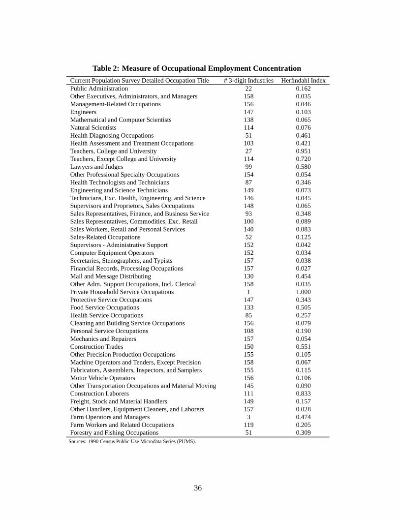
Table 2: Measure of Occupational Employment Concentration

Current Population Survey Detailed Occupation Title # 3-digit Industries Herfindahl IndexPublic Administration 22 0.162Other Executives, Administrators, and Managers 158 0.035Management-Related Occupations 156 0.046Engineers 147 0.103Mathematical and Computer Scientists 138 0.065Natural Scientists 114 0.076Health Diagnosing Occupations 51 0.461Health Assessment and Treatment Occupations 103 0.421Teachers, College and University 27 0.951Teachers, Except College and University 114 0.720Lawyers and Judges 99 0.580Other Professional Specialty Occupations 154 0.054Health Technologists and Technicians 87 0.346Engineering and Science Technicians 149 0.073Technicians, Exc. Health, Engineering, and Science 146 0.045Supervisors and Proprietors, Sales Occupations 148 0.065Sales Representatives, Finance, and Business Service 93 0.348Sales Representatives, Commodities, Exc. Retail 100 0.089Sales Workers, Retail and Personal Services 140 0.083Sales-Related Occupations 52 0.125Supervisors - Administrative Support 152 0.042Computer Equipment Operators 152 0.034Secretaries, Stenographers, and Typists 157 0.038Financial Records, Processing Occupations 157 0.027Mail and Message Distributing 130 0.454Other Adm. Support Occupations, Incl. Clerical 158 0.035Private Household Service Occupations 1 1.000Protective Service Occupations 147 0.343Food Service Occupations 133 0.505Health Service Occupations 85 0.257Cleaning and Building Service Occupations 156 0.079Personal Service Occupations 108 0.190Mechanics and Repairers 157 0.054Construction Trades 150 0.551Other Precision Production Occupations 155 0.105Machine Operators and Tenders, Except Precision 158 0.067Fabricators, Assemblers, Inspectors, and Samplers 155 0.115Motor Vehicle Operators 156 0.106Other Transportation Occupations and Material Moving 145 0.090Construction Laborers 111 0.833Freight, Stock and Material Handlers 149 0.157Other Handlers, Equipment Cleaners, and Laborers 157 0.028Farm Operators and Managers 3 0.474Farm Workers and Related Occupations 119 0.205Forestry and Fishing Occupations 51 0.309

Sources: 1990 Census Public Use Microdata Series (PUMS).

36

Table 3: Sample Statistics

Variables All sample Stayers SwitchersAge 28.12 27.56 26.63

(0.11) (0.24) (0.17)White 79.94% 84.43% 76.53%Married 45.26% 40.86% 52.00%Years Schooling 12.19 11.86 12.03

(0.06) (0.10) (0.11)HS 70.30% 72.62% 68.80%College 8.63% 4.18% 7.50%Experience 5.02 4.68 3.81

(0.10) (0.21) (0.14)Tenure 1.34 1.62 0.86

(0.07) (0.18) (0.04)Received UI 41.32% 55.49% 34.39%Displaced 19.93% 14.24% 24.40%Number of spells 5,425 1,479 1,158N. of clusters 2,251 756 746

Notes: (1) Standard deviations are in parentheses; (2) 2,741 unemployment spells (outof 5,344) did not report occupational code either for the previous or the new job or both.Source: NLSY79, 1979-2000.

Table 4: Unemployment Duration: Cox PH Estimated Hazards

Same Occupation Different Occupationcoef. std coef. std

OER 0.743 (0.124)†* 0.981 (0.196)White 1.446 (0.132)** 0.992 (0.085)Age 0.769 (0.143) 1.149 (0.257)Age2 1.004 (0.003) 0.996 (0.004)Ability Factor 1 1.031 (0.021) 1.009 (0.018)Ability Factor 12 0.997 (0.006) 0.997 (0.004)Ability Factor 2 1.049 (0.044) 0.932 (0.042)Ability Factor 22 1.017 (0.031) 0.974 (0.032)High school 1.034 (0.099) 1.012 (0.090)College 0.434 (0.120)** 0.918 (0.159)Married 0.920 (0.072) 1.020 (0.082)Experience 1.147 (0.070)* 1.061 (0.074)Experience2 0.992 (0.004)† 1.000 (0.006)Tenure 1.231 (0.063)** 0.823 (0.061)**Tenure2 0.989 (0.005)* 1.014 (0.010)Unemployment Insurance1.228 (0.095)** 0.727 (0.059)**Unemp. Rate 1.000 (0.016) 0.973 (0.013)*N. of spells 4,929 4,929N. of clusters 2,065 2,065Wald chi2(17) 121.42 48.08

**, *, †: significant at 1%, 5%, and 10%, respectively; †*: significant at 8%. Notes: (1) Standard deviationsare in parentheses; (2) Ability factors 1 and 2 are principalcomponents the first two of the age-adjusted

ASVAB scores. Source: NLSY79, 1979-2000.

37

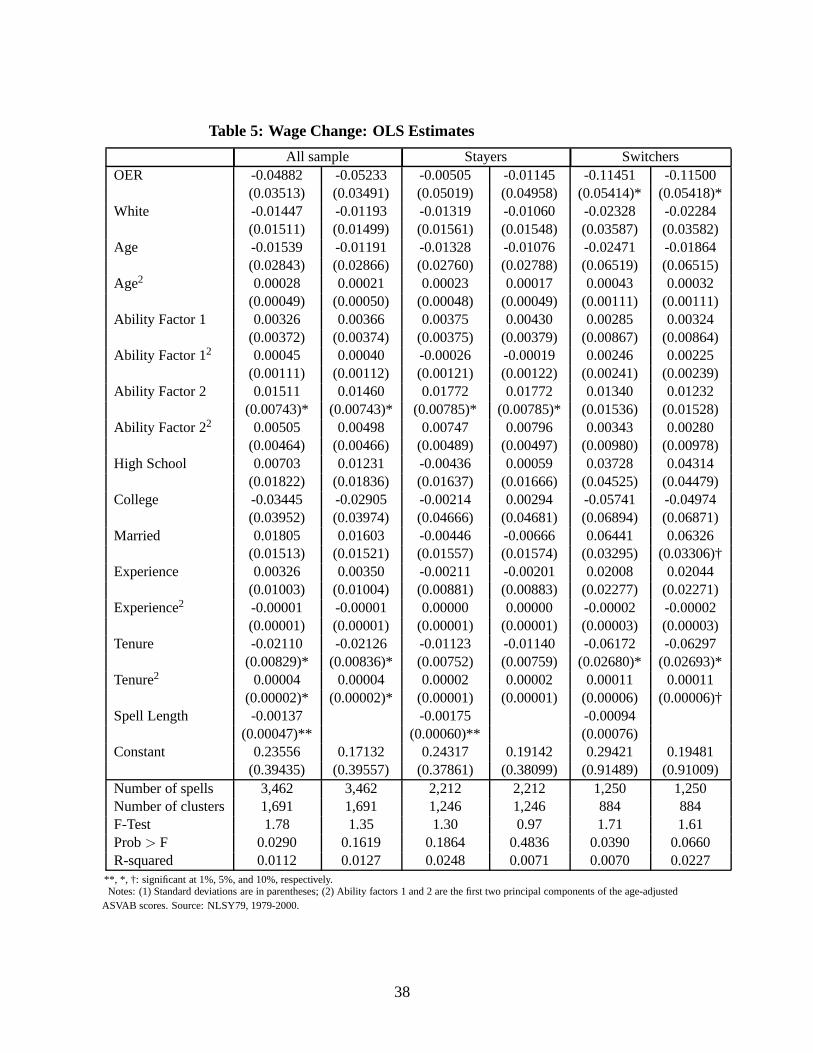
Table 5: Wage Change: OLS Estimates

All sample Stayers SwitchersOER -0.04882 -0.05233 -0.00505 -0.01145 -0.11451 -0.11500

(0.03513) (0.03491) (0.05019) (0.04958) (0.05414)* (0.05418)*White -0.01447 -0.01193 -0.01319 -0.01060 -0.02328 -0.02284

(0.01511) (0.01499) (0.01561) (0.01548) (0.03587) (0.03582)Age -0.01539 -0.01191 -0.01328 -0.01076 -0.02471 -0.01864

(0.02843) (0.02866) (0.02760) (0.02788) (0.06519) (0.06515)Age2 0.00028 0.00021 0.00023 0.00017 0.00043 0.00032

(0.00049) (0.00050) (0.00048) (0.00049) (0.00111) (0.00111)Ability Factor 1 0.00326 0.00366 0.00375 0.00430 0.00285 0.00324

(0.00372) (0.00374) (0.00375) (0.00379) (0.00867) (0.00864)Ability Factor 12 0.00045 0.00040 -0.00026 -0.00019 0.00246 0.00225

(0.00111) (0.00112) (0.00121) (0.00122) (0.00241) (0.00239)Ability Factor 2 0.01511 0.01460 0.01772 0.01772 0.01340 0.01232

(0.00743)* (0.00743)* (0.00785)* (0.00785)* (0.01536) (0.01528)Ability Factor 22 0.00505 0.00498 0.00747 0.00796 0.00343 0.00280

(0.00464) (0.00466) (0.00489) (0.00497) (0.00980) (0.00978)High School 0.00703 0.01231 -0.00436 0.00059 0.03728 0.04314

(0.01822) (0.01836) (0.01637) (0.01666) (0.04525) (0.04479)College -0.03445 -0.02905 -0.00214 0.00294 -0.05741 -0.04974

(0.03952) (0.03974) (0.04666) (0.04681) (0.06894) (0.06871)Married 0.01805 0.01603 -0.00446 -0.00666 0.06441 0.06326

(0.01513) (0.01521) (0.01557) (0.01574) (0.03295) (0.03306)†Experience 0.00326 0.00350 -0.00211 -0.00201 0.02008 0.02044

(0.01003) (0.01004) (0.00881) (0.00883) (0.02277) (0.02271)Experience2 -0.00001 -0.00001 0.00000 0.00000 -0.00002 -0.00002

(0.00001) (0.00001) (0.00001) (0.00001) (0.00003) (0.00003)Tenure -0.02110 -0.02126 -0.01123 -0.01140 -0.06172 -0.06297

(0.00829)* (0.00836)* (0.00752) (0.00759) (0.02680)* (0.02693)*Tenure2 0.00004 0.00004 0.00002 0.00002 0.00011 0.00011

(0.00002)* (0.00002)* (0.00001) (0.00001) (0.00006) (0.00006)†Spell Length -0.00137 -0.00175 -0.00094

(0.00047)** (0.00060)** (0.00076)Constant 0.23556 0.17132 0.24317 0.19142 0.29421 0.19481

(0.39435) (0.39557) (0.37861) (0.38099) (0.91489) (0.91009)Number of spells 3,462 3,462 2,212 2,212 1,250 1,250Number of clusters 1,691 1,691 1,246 1,246 884 884F-Test 1.78 1.35 1.30 0.97 1.71 1.61Prob> F 0.0290 0.1619 0.1864 0.4836 0.0390 0.0660R-squared 0.0112 0.0127 0.0248 0.0071 0.0070 0.0227

**, *, †: significant at 1%, 5%, and 10%, respectively.Notes: (1) Standard deviations are in parentheses; (2) Ability factors 1 and 2 are the first two principal components of the age-adjusted

ASVAB scores. Source: NLSY79, 1979-2000.

38

Figure 1: Average Unemployment Duration by Occupation

*Occupations omitted from the graph had no observations.

Managerial &

Professional

Tech., Sales

& Clerical

Production,

Craft & Repair

Farming,

Forestry &

Fishing

Operators,

Fabricators &

Laborers

Services

0

2

4

6

8

10

12

14

16

18

20

22

1 2 3 4 5 6 7 8 9 10 11 12 13 14 15 17 18 19 21 22 23 24 25 26 27 28 29 30 31 32 33 34 35 36 37 38 39 40 41 42 43 44 45

Weeks

Mean

Source: NLSY79, 1979-2000.

1. Public Administration 2. Other Executives, Administrators, and Managers

3. Management-Related Occupations 4. Engineers

5. Mathematical and Computer Scientists 6. Natural Scientists

7. Health Diagnosing Occupations 8. Health Assessment and Treatment Occupations

9. Teachers, College and University 10. Teachers, Except College and University

11. Lawyers and Judges 12. Other Professional Specialty Occupations

13. Health Technologists and Technicians 14. Engineering and Science Technicians

15. Technicians, Exc. Health, Eng. and Science 16. Supervisors and Proprietors, Sales Occps.

17. Sales Repres., Finance, and Business Service 18. Sales Repres., Commodities, Exc. Retail

19. Sales Workers, Retail and Personal Services 20. Sales-Related Occupations

21. Supervisors - Administrative Support 22. Computer Equipment Operators

23. Secretaries, Stenographers, and Typists 24. Financial Records, Processing Occupations

25. Mail and Message Distributing 26. Other Administrative Support, Incl. Clerical

27. Private Household Service Occupations 28. Protective Service Occupations

29. Food Service Occupations 30. Health Service Occupations

31. Cleaning and Building Service Occupations 32. Personal Service Occupations

33. Mechanics and Repairers 34. Construction Trades

35. Other Precision Production Occupations 36. Machine Operators & Tenders, Exc. Precision

37. Fabricators, Assemblers, Inspec. & Samplers 38. Motor Vehicle Operators

39. Other Transportation & Material Moving Occps 40. Construction Laborers

41. Freight, Stock and Material Handlers 42. Other Handlers, Equip. Cleaners, & Laborers

43. Farm Operators and Managers 44. Farm Workers and Related Occupations

45. Forestry and Fishing Occupations

Source: NLSY79, 1979-2000.

39

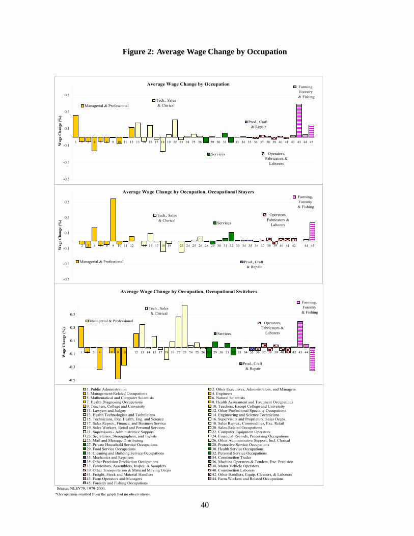
Figure 2: Average Wage Change by Occupation

*Occupations omitted from the graph had no observations.

Average Wage Change by Occupation, Occupational Stayers

Managerial & Professional

Tech., Sales

& Clerical

Operators,

Fabricators &

Laborers

Prod., Craft

& Repair

Farming,

Forestry

& Fishing

Services

-0.5

-0.3

-0.1

0.1

0.3

0.5

2 3 4 5 8 9 10 11 12 14 15 17 18 19 23 24 25 26 28 29 30 31 32 33 34 35 36 37 38 39 40 41 42 44 45

Wa

ge

Ch

an

ge

(%)

Average Wage Change by Occupation, Occupational Switchers

Services

Farming,

Forestry

& Fishing

Prod., Craft

& Repair

Operators,

Fabricators &

Laborers

Tech., Sales

& Clerical

Managerial & Professional

-0.5

-0.3

-0.1

0.1

0.3

0.5

1 2 3 4 8 9 10 12 13 14 15 17 18 19 22 23 24 25 26 28 29 30 31 32 33 34 35 36 37 38 39 40 41 42 43 44 45

Wa

ge

Ch

an

ge

(%)

Source: NLSY79, 1979-2000.

Average Wage Change by Occupation

Services

Farming,

Forestry

& Fishing

Prod., Craft

& Repair

Operators,

Fabricators &

Laborers

Tech., Sales

& ClericalManagerial & Professional

-0.5

-0.3

-0.1

0.1

0.3

0.5

1 2 3 4 5 8 9 10 11 12 13 14 15 17 18 19 22 23 24 25 26 28 29 30 31 32 33 34 35 36 37 38 39 40 41 42 43 44 45

Wa

ge

Ch

an

ge

(%)

1. Public Administration 2. Other Executives, Administrators, and Managers3. Management-Related Occupations 4. Engineers5. Mathematical and Computer Scientists 6. Natural Scientists7. Health Diagnosing Occupations 8. Health Assessment and Treatment Occupations9. Teachers, College and University 10. Teachers, Except College and University11. Lawyers and Judges 12. Other Professional Specialty Occupations13. Health Technologists and Technicians 14. Engineering and Science Technicians15. Technicians, Exc. Health, Eng. and Science 16. Supervisors and Proprietors, Sales Occps.17. Sales Repres., Finance, and Business Service 18. Sales Repres., Commodities, Exc. Retail19. Sales Workers, Retail and Personal Services 20. Sales-Related Occupations21. Supervisors - Administrative Support 22. Computer Equipment Operators23. Secretaries, Stenographers, and Typists 24. Financial Records, Processing Occupations25. Mail and Message Distributing 26. Other Administrative Support, Incl. Clerical27. Private Household Service Occupations 28. Protective Service Occupations29. Food Service Occupations 30. Health Service Occupations31. Cleaning and Building Service Occupations 32. Personal Service Occupations33. Mechanics and Repairers 34. Construction Trades35. Other Precision Production Occupations 36. Machine Operators & Tenders, Exc. Precision37. Fabricators, Assemblers, Inspec. & Samplers 38. Motor Vehicle Operators39. Other Transportation & Material Moving Occps 40. Construction Laborers41. Freight, Stock and Material Handlers 42. Other Handlers, Equip. Cleaners, & Laborers43. Farm Operators and Managers 44. Farm Workers and Related Occupations45. Forestry and Fishing Occupations

40

Figure 3: Accountants and Earth Drillers Employment Distri bution across Industries

!"# $%#

!"# $%#

Source:1990 Census Public Use Microdata Series(PUMS).

41

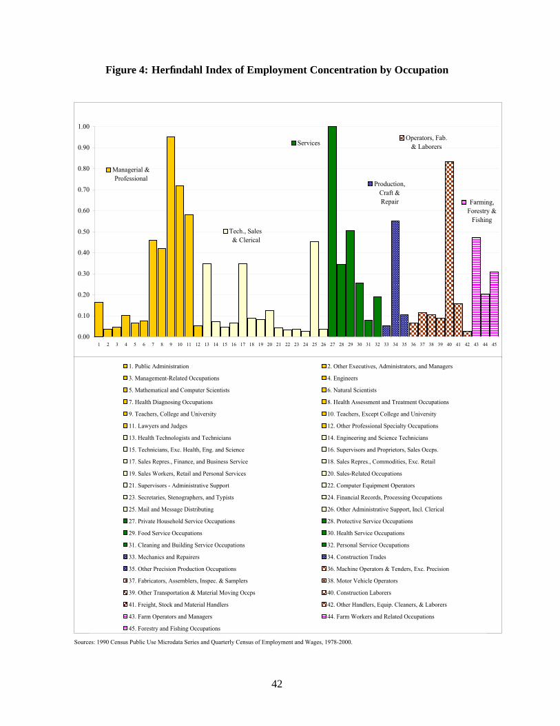
Figure 4: Herfindahl Index of Employment Concentration by Occupation

Operators, Fab.

& Laborers

Farming,

Forestry &

Fishing

Production,

Craft &

Repair

Services

Tech., Sales

& Clerical

Managerial &

Professional

0.00

0.10

0.20

0.30

0.40

0.50

0.60

0.70

0.80

0.90

1.00

1 2 3 4 5 6 7 8 9 10 11 12 13 14 15 16 17 18 19 20 21 22 23 24 25 26 27 28 29 30 31 32 33 34 35 36 37 38 39 40 41 42 43 44 45

Sources: 1990 Census Public Use Microdata Series and Quarterly Census of Employment and Wages, 1978-2000.

1. Public Administration 2. Other Executives, Administrators, and Managers

3. Management-Related Occupations 4. Engineers

5. Mathematical and Computer Scientists 6. Natural Scientists

7. Health Diagnosing Occupations 8. Health Assessment and Treatment Occupations

9. Teachers, College and University 10. Teachers, Except College and University

11. Lawyers and Judges 12. Other Professional Specialty Occupations

13. Health Technologists and Technicians 14. Engineering and Science Technicians

15. Technicians, Exc. Health, Eng. and Science 16. Supervisors and Proprietors, Sales Occps.

17. Sales Repres., Finance, and Business Service 18. Sales Repres., Commodities, Exc. Retail

19. Sales Workers, Retail and Personal Services 20. Sales-Related Occupations

21. Supervisors - Administrative Support 22. Computer Equipment Operators

23. Secretaries, Stenographers, and Typists 24. Financial Records, Processing Occupations

25. Mail and Message Distributing 26. Other Administrative Support, Incl. Clerical

27. Private Household Service Occupations 28. Protective Service Occupations

29. Food Service Occupations 30. Health Service Occupations

31. Cleaning and Building Service Occupations 32. Personal Service Occupations

33. Mechanics and Repairers 34. Construction Trades

35. Other Precision Production Occupations 36. Machine Operators & Tenders, Exc. Precision

37. Fabricators, Assemblers, Inspec. & Samplers 38. Motor Vehicle Operators

39. Other Transportation & Material Moving Occps 40. Construction Laborers

41. Freight, Stock and Material Handlers 42. Other Handlers, Equip. Cleaners, & Laborers

43. Farm Operators and Managers 44. Farm Workers and Related Occupations

45. Forestry and Fishing Occupations

42

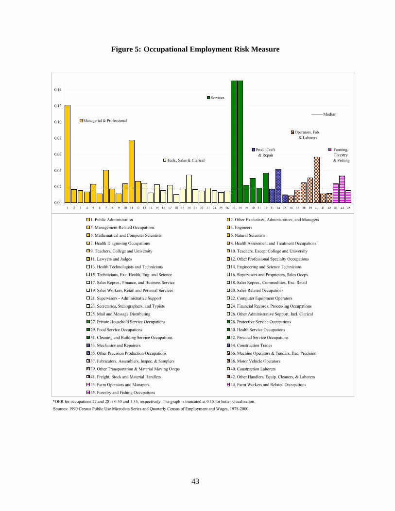
Figure 5: Occupational Employment Risk Measure

*OER for occupations 27 and 28 is 0.30 and 1.35, respectively. The graph is truncated at 0.15 for better visualization.

Managerial & Professional

Tech., Sales & Clerical

Prod., Craft

& Repair

Services

Farming,

Forestry

& Fishing

Operators, Fab.

& Laborers

0.00

0.02

0.04

0.06

0.08

0.10

0.12

0.14

1 2 3 4 5 6 7 8 9 10 11 12 13 14 15 16 17 18 19 20 21 22 23 24 25 26 27 28 29 30 31 32 33 34 35 36 37 38 39 40 41 42 43 44 45

Median

Sources: 1990 Census Public Use Microdata Series and Quarterly Census of Employment and Wages, 1978-2000.

1. Public Administration 2. Other Executives, Administrators, and Managers

3. Management-Related Occupations 4. Engineers

5. Mathematical and Computer Scientists 6. Natural Scientists

7. Health Diagnosing Occupations 8. Health Assessment and Treatment Occupations

9. Teachers, College and University 10. Teachers, Except College and University

11. Lawyers and Judges 12. Other Professional Specialty Occupations

13. Health Technologists and Technicians 14. Engineering and Science Technicians

15. Technicians, Exc. Health, Eng. and Science 16. Supervisors and Proprietors, Sales Occps.

17. Sales Repres., Finance, and Business Service 18. Sales Repres., Commodities, Exc. Retail

19. Sales Workers, Retail and Personal Services 20. Sales-Related Occupations

21. Supervisors - Administrative Support 22. Computer Equipment Operators

23. Secretaries, Stenographers, and Typists 24. Financial Records, Processing Occupations

25. Mail and Message Distributing 26. Other Administrative Support, Incl. Clerical

27. Private Household Service Occupations 28. Protective Service Occupations

29. Food Service Occupations 30. Health Service Occupations

31. Cleaning and Building Service Occupations 32. Personal Service Occupations

33. Mechanics and Repairers 34. Construction Trades

35. Other Precision Production Occupations 36. Machine Operators & Tenders, Exc. Precision

37. Fabricators, Assemblers, Inspec. & Samplers 38. Motor Vehicle Operators

39. Other Transportation & Material Moving Occps 40. Construction Laborers

41. Freight, Stock and Material Handlers 42. Other Handlers, Equip. Cleaners, & Laborers

43. Farm Operators and Managers 44. Farm Workers and Related Occupations

45. Forestry and Fishing Occupations

43