1

DISTRIBUTION STATEMENT A. Approved for public release; distribution is unlimited.

Ocean Basin Impact of Ambient Noise on Marine Mammal Detectability, Distribution, and Acoustic Communication - YIP

Jennifer L. Miksis-Olds

Applied Research Laboratory The Pennsylvania State University

PO Box 30 Mailstop 3510D State College, PA 16804

phone: (814) 865-9318 fax: (814) 863-8783 email: jlm91@psu.edu

Award Number: N000141110619

LONG-TERM GOALS The ultimate goal of this research is to enhance the understanding of global ocean noise and how variability in sound level impacts marine mammal acoustic communication and detectability. How short term variability and long term changes of ocean basin acoustics impact signal detection will be considered by examining 1) the variability in low-frequency ocean sound levels and sources, and 2) the relationship of sound variability on signal detections as it relates to marine mammal active acoustic space and acoustic communication. This work increases the spatial range and time scale of prior studies conducted at a local or regional scale. The comparison of acoustic time series from different ocean basins provides a synoptic perspective for observing and monitoring ocean noise on multiple times scales in both hemispheres as economic and climate conditions change. Quantified changes in the acoustic environment can then be applied to the investigation of ocean noise issues related to general signal detection tasks, as well as marine mammal acoustic communication and impacts. OBJECTIVES The growing concern that ambient ocean sound levels are increasing and could impact signal detection of important acoustic signals being used by animals for communication and by humans for military and mitigation purposes will be addressed. The overall goal of the study is to gain a better understanding of how low frequency sound levels vary over space and time. This knowledge will then be related to the range over which marine mammal vocalizations can be detected over different time scales and seasons. Over a decade of passive acoustic time series from the Indian and Pacific Oceans will be used to address the following project objectives: 1. Determine the major sources (or drivers) of variation in low frequency ambient sound levels

on a regional and ocean basin scale. A. What are the regional source contributions to low frequency ambient sound levels?

B. Is there variation in source characteristics of the major low frequency source components over space and time?

C. Is low frequency sound level uniformly increasing on a global scale?

Report Documentation Page Form ApprovedOMB No. 0704-0188

Public reporting burden for the collection of information is estimated to average 1 hour per response, including the time for reviewing instructions, searching existing data sources, gathering andmaintaining the data needed, and completing and reviewing the collection of information. Send comments regarding this burden estimate or any other aspect of this collection of information,including suggestions for reducing this burden, to Washington Headquarters Services, Directorate for Information Operations and Reports, 1215 Jefferson Davis Highway, Suite 1204, ArlingtonVA 22202-4302. Respondents should be aware that notwithstanding any other provision of law, no person shall be subject to a penalty for failing to comply with a collection of information if itdoes not display a currently valid OMB control number.

1. REPORT DATE 30 SEP 2013 2. REPORT TYPE

3. DATES COVERED 00-00-2013 to 00-00-2013

4. TITLE AND SUBTITLE Ocean Basin Impact of Ambient Noise on Marine Mammal Detectability,Distribution, and Acoustic Communication - YIP

5a. CONTRACT NUMBER

5b. GRANT NUMBER

5c. PROGRAM ELEMENT NUMBER

6. AUTHOR(S) 5d. PROJECT NUMBER

5e. TASK NUMBER

5f. WORK UNIT NUMBER

7. PERFORMING ORGANIZATION NAME(S) AND ADDRESS(ES) Pennsylvania State University,Applied Research Laboratory,PO Box30,State College,PA,16804

8. PERFORMING ORGANIZATIONREPORT NUMBER

9. SPONSORING/MONITORING AGENCY NAME(S) AND ADDRESS(ES) 10. SPONSOR/MONITOR’S ACRONYM(S)

11. SPONSOR/MONITOR’S REPORT NUMBER(S)

12. DISTRIBUTION/AVAILABILITY STATEMENT Approved for public release; distribution unlimited

13. SUPPLEMENTARY NOTES

14. ABSTRACT

15. SUBJECT TERMS

16. SECURITY CLASSIFICATION OF: 17. LIMITATION OF ABSTRACT Same as

Report (SAR)

18. NUMBEROF PAGES

20

19a. NAME OFRESPONSIBLE PERSON

a. REPORT unclassified

b. ABSTRACT unclassified

c. THIS PAGE unclassified

Standard Form 298 (Rev. 8-98) Prescribed by ANSI Std Z39-18

2

2. Investigate the impacts of variation in low frequency ambient sound levels on signal detection range, marine mammal communication, and distribution.

A. How does species specific detection range (acoustic active space) vary on a daily, weekly, monthly, and yearly time scale?

B. Are low-frequency vocalization detections related to changes in ambient sound level?

C. Do marine mammals exhibit any changes in calling behavior to compensate for noise?

APPROACH The originally proposed effort was a comparative study of passive acoustic time series from the Comprehensive Nuclear Test Ban Treaty Organization International Monitoring System (CTBTO IMS) locations in the Indian (H08) and Pacific (H11) Oceans over the past decade (Figure 1, Table 1). An additional site at Ascension Island (H10) in the Atlantic Ocean was added because it provides an additional southern hemisphere site for comparing noise trends to the Wake Island site in the northern hemisphere (Figure 1, Table 1). CTBTO monitoring stations consist of two sets of three omni-directional hydrophones (0.002-125 Hz) on opposite sides of an island. Two triads of hydrophones eliminate the acoustic shadow created by the island to ensure full area coverage of an ocean basin. The hydrophones are located in the SOFAR channel at a depth of 600 to 1200 m, depending on location. The hydrophones are cabled to land 50-100 km away and connected to shore stations for data transmission. The sites are under the national control of the countries to which the hydrophones are cabled and data is available via AFTAC/US NDC (Air Force Tactical Applications Center/ US National Data Center) for US citizens. Individual datasets are calibrated to absolute sound pressure levels (SPL) in standard SI units, removing site-specific hydrophone responses. Many of the acoustic signals present have been well characterized for various species of marine mammals, physical events, and anthropogenic sources such as seismic array signals, allowing for development of automated spectrogram correlation detectors that are being run on long batches of recorded data to detect the presence of sounds produced by particular species or sources (i.e. Mellinger & Clark, 2000, 2006). These automated detection methods make it practical to survey the large dataset in this study which would be prohibitively time consuming for a manual search. The cornerstone of project success is the appropriate time series analyses and comparisons over time at a single location and across locations. While there is great scientific merit in quantifying the acoustic relationship between physical and biological parameters of the marine ecosystem, the integration of the acoustic datasets with ancillary data sets further enhances the value of the research by ensuring the appropriate comparisons are made between locations and over time at the same location. Remotely sensed chorolophyll concentration and sea surface temperature are being modeled for the targeted ocean regions to provide insight on the level of primary productivity within each area. Historical vessel data and movements were purchased through Lloyd’s Marine Intelligence Unit (MIU). The database extends back to 1997, which is appropriate for obtaining shipping data over the same time periods and scales of the acoustic data and other ancillary datasets. An initial key question that must be addressed when interpreting passively collected ambient noise is: “What is the most appropriate unit of analysis or size window over which the data is being examined?” Long-term analyses of ambient sound levels require particular care in selecting the unit of analysis

3

because sources contribute to the ambient sound level on different time and spatial scales. The optimal unit of analysis and sub-sampling interval should capture the true variation of the system while excluding redundant data in order to minimize processing time (Curtis et al., 1999). Data processing in previous ambient sound studies range from using all data acquired with continuously recording systems to sparsely subsampled data from remotely deployed autonomous systems. There are currently no standards for sub-sampling intervals, averaging window lengths, or other parameters related to the analysis of long-term ambient noise data, which is necessary in order to compare and interpret data sets recorded from different systems, in different places, and at different times. The unit of analyses that have been previously used in ambient sound studies was either arbitrarily selected, defined by system limitations, or selected based on criteria other than results of statistical tests exploring the data variability. Hence, one of this year’s project efforts focused on developing methods to identify the optimal unit of analysis for data from a single location (H08 in the Indian Ocean) by determining at what point sub-sampling of the ambient sound level caused a significant deviation from the actual sound level. Results of this effort are being applied to the analysis of ambient sound data from the other two oceans, used in the development of mixed-models to identify significant drivers of ambient sound variability, and translated to calculations of detection ranges for defining the relationship of sound variability on signal detection as it relates to marine mammal active acoustic space and acoustic communication. A second focus of this year’s efforts applied knowledge gained from the unit of analysis results to the examination of ambient sound levels over time. Deep water ambient sound levels have increased in the North Pacific Ocean over the past 60 years (Ross, 1993, 2005; Andrew et al., 2002; McDonald et al., 2006; Chapman and Price, 2011). The rate of increase was measured at approximately 3 dB/decade (0.55 dB/yr) up until the 1980s and then slowed to 0.2 dB/yr. The rising sound levels in the North Pacific have sparked concern about the related environmental impacts as well as whether these trends are indicative of global sound level increases. Very recent studies have started to contribute information from locations outside the North Pacific to answer the question of whether the trends observed in the North Pacific are indicative of an overall global or hemispheric increase in low frequency ambient noise (Van der Schaar et al., 2013; Miksis-Olds et al., 2013). This on-going work selectively decomposed the long-term time series by frequency and sound level percentile to provide insight relating to conditions ranging from the quietest conditions (sound floor) to the most extreme acoustic events in the Indian, South Atlantic, and Equatorial Pacific Ocean. Rate, direction, and magnitude of changes were examined within each percentile as opposed to using the percentiles as only a means to estimate and display variance. WORK COMPLETED Research efforts this past year focused on: 1) identifying the optimal unit of analysis for processing long-term acoustic time series, 2) assessing long-term patterns and trends in ambient sound level at the three CTBTO IMS locations, 3) developing a rapid acoustic survey method to assess biodiversity, and 4) generating acoustic, shipping, and oceanographic time series needed to develop predictive models of ambient sound and signal detection ranges. Data from three different CTBTO sites have been downloaded from the AFTAC/US NDC to ARL Penn State. The site locations and current data acquisition are shown in Table 2. Data continues to be downloaded on a monthly basis to keep the database current. In-depth analysis of the acoustic time series at Diego Garcia was conducted to identify the point at which longer averaging windows and sub-sampling intervals result in a significant deviation from the

4

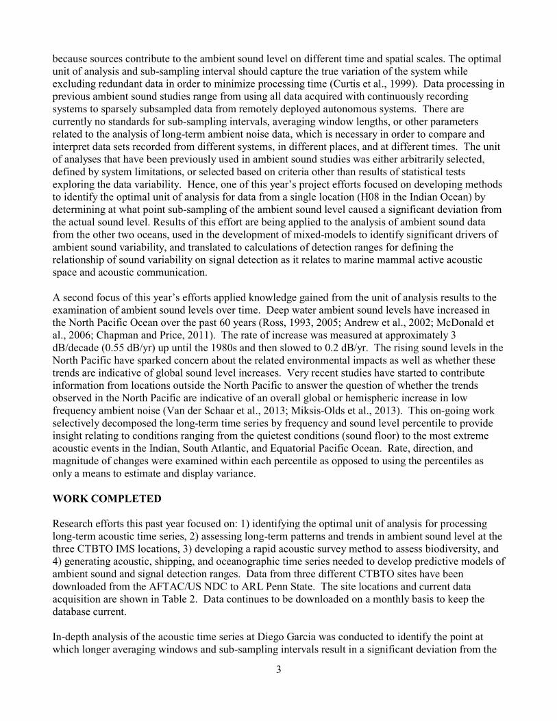
actual sound levels and variation. Mean rank and sound level probability distributions were assessed for differences across window lengths of 10, 15, 30, 60, and 200 s. The subsampling analysis examined mean rank and sound level probability distribution difference at 5 subsampling intervals. Sixty second averages were sub-sampled at intervals of 1, 5, 10, 30, and 60 minutes, and 200s averages were subsampled at 3.3, 10, 16.6, 33.3, and 50 min intervals. Sound levels were estimated for the full CTBTO spectrum and three 20-Hz bandwidths: 10-30 Hz, 40-60 Hz, and 85-105 Hz. The 10-30 Hz band was selected as representative of low frequency vocalizations from large whales (e.g. blue and fin whales). The 40-60 Hz band reflects energy contributions from shipping, animal vocalizations, and seismic airguns making this a “transitional” band. The 85-105 Hz band was selected as representative of the dominant frequencies of distant shipping. Differences in the mean ranks of the average sound level across subsampling intervals and window lengths within each frequency category were assessed with a Kurskal-Wallis test, a nonparametric generalization of the ANOVA appropriate for non-Gaussian data (Lix et al., 1996). Based on the unit of analysis results from Diego Garcia, time series of daily averages were calculated for all sites from the date of site inception to January 2013. Mean spectral levels were calculated using a 15,000 point DFT Hann window and no overlap to produce sequential 1-min power spectrum estimates over the duration of the datasets. Averages were computed using intensity levels and were then converted back to dB units. Five daily percentile parameters (P1, P10, P50, P90, P99) were identified from 1440 one-minute power spectrum estimates calculated each day. Each daily percentile value represents the level below which a certain percent of measurements fall within a single day. The P1 value is representative of the sound floor (quietest ambient conditions). The P50 value is the daily median, and the P99 value reflects the most extreme sound levels occurring within a day. Acoustic trends were assessed using all data available from the date of inception at each island location to 11 January 2013 (Table 1). A linear regression model of sound level with date was fit for each of the time series to explore the long-term trend of the sound level. No inferential conclusions were drawn from the linear regression models due to the non-Gaussian distribution and serial correlation of the data. Initial exploration and development of methods to measure biodiversity at each CTBTO IMS locations was assessed for a week long time series at each of the three location in each season over the course of a year. An acoustic biodiversity index following the procedure in Sueur et al. (2008) was computed using a custom script written in MATLAB. Temporal (Ht) and spectral (Hf) acoustic entropies were computed and then multiplied to obtain the acoustic biodiversity index (H). The spectral entropy calculation used a Fourier transform window length of 1024 points resulting in a frequency resolution of 0.25 Hz. Acoustic entropy values were generated over one hour time periods from 01-02 Jan at the H08-Indian Ocean location as a detailed exploration to determine how reflective the acoustic entropy values were of biodiversity in the marine environment. The detailed exploration of data on 01-02 Jan 2008 produced time series of hourly whale calls, seismic activity, and entropy estimates. Initial analyses revealed that the entropy values were highly influenced by the presence of anthropogenic seismic exploration signals on 02 Jan and not consistent with the level of biodiversity observed over the same time period (Figure 2a) hence, a method of removing the influence of anthropogenic seismic signals through a background removal technique was developed (Bendat and Piersol, 2000; Wu and Jeng, 2002). The presence of anthropogenic seismic exploration signals was compensated for by creating an average complex spectrum of characteristic seismic exploration signals. The window length of the average spectrum was the same as the window for the calculation of the biodiversity index (1024 points). The seismic spectrum was subtracted from the average spectra of each period analyzed that

5

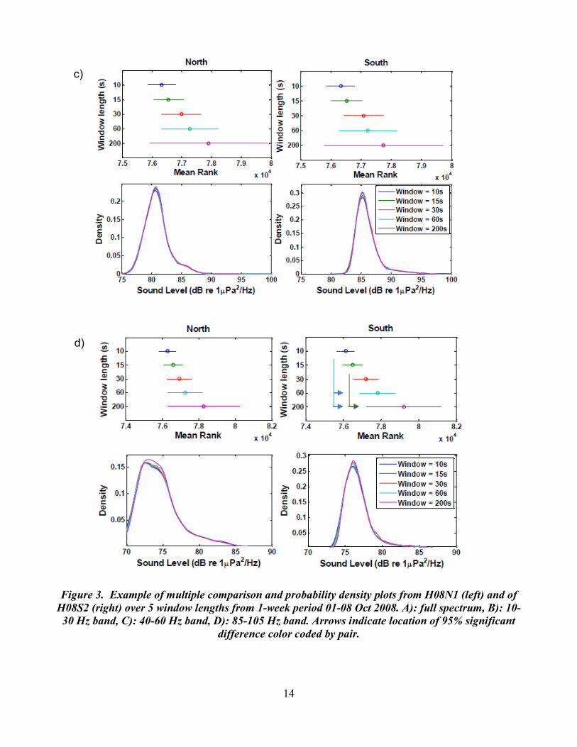
contained seismic signals. The spectral entropy (Hf ) was then recalculated using this adjusted spectrum when the analysis period contained seismic exploration signals and the default spectral entropy when no seismic was present. The combined compensated entropy values was denoted as HN and more accurately reflected changes in the acoustic activity of biological sound sources (Figure 2b). Acoustic entropy values (H and HN) were generated over six hour time periods for each week long time series at each location and in each season (4 time periods x 7 days x 4 seasons x 3 locations) for a total of 336 analysis periods. Six hour time periods were selected to be consistent with the temporal scale of the classified biologic signals and reflective of daily photoperiods (00:00-6:00, 6:00-12:00, 12:00-18:00, 18:00-24:00). Comparisons within and between sites and seasons were assessed using a nonparametric Kruskal-Wallis test. The Kruskal-Wallis test determines whether the mean ranks of distributions are equal across different categories. This test was used to test the null hypothesis that acoustic diversity (HN) was equal across sites and seasons. RESULTS Unit of analysis Results illustrate the degree of uncertainty in sound levels based on different units of analysis. The window length analysis was performed over 10 randomized 1-week time periods on both H08N1 and H08S2 throughout the decade spanning 2002 to 2012. The mean ranks at both H08N1 and H08S2 were not equal over the five window lengths examined (10, 15, 30, 60, and 200 s) (N1: X2= 62.7, df=4, p < 0.001, S2: X2 = 47.9, df=4, p < 0.001) (Figure 3). The results of the ten randomized tests showed that 100% of the tests over the 10-30 Hz band showed significant differences between the mean sound pressure levels over the different temporal windows, and 80% of the tests over the 5-110 Hz band showed significant differences. The 40-60 Hz and 85-105 Hz bands showed no significant differences in mean sound level across the temporal window the majority of the time. 90% of the tests over the 85-105 Hz band showed no significant difference, and 70% of the tests over the 40-60 Hz band showed no significant difference. The largest difference between the maximum and minimum sound level estimates as a function of window length over all analyses was approximately 1 dB re 1 μPa2/Hz, and larger windows were more susceptible to variation due to subsampling; hence a 60 second window length was used for subsequent analyses of patterns and trends over long time periods. [Full details of this work can be found in the MS Thesis by Russell Hawkins (Hawkins, 2013) and in the resulting publications submitted to JASA (Hawkins & Miksis-Olds, 2013). The subsampling interval analyses tested the null hypothesis that mean ranks and distributions of data were equal over five subsampling intervals. The analysis was conducted twice using a short window length (60 s) with subsampling intervals of 1, 5, 15, 30, and 60 min, and a long window length (200 s) with subsampling intervals of 3.3, 10, 16.6, 33.3, and 50 min. The overall trend direction observed in each frequency category and for each of the two window lengths was that mean rank of the average sound level decreased with longer subsampling intervals (Figure 4).The subsampling interval analyses were performed over 100 randomized 6-week periods throughout the decade, and differences in the mean ranks of the average sound level across subsampling intervals within each frequency category were assessed with a Kruskal-Wallis test (Figure 5). Significance of the observed proportions was tabulated via a normalized cumulative probability density function. The average difference between sound level estimates in the 10-30 Hz band due to subsampling was 2 dB re 1 μPa2/Hz and as high as 4 dB re 1 μPa2/Hz. The average difference in the full band (5-110 Hz) was approximately 1 dB re 1 μPa2/Hz and as high as 6 dB re 1 μPa2/Hz (Figure 6).

6

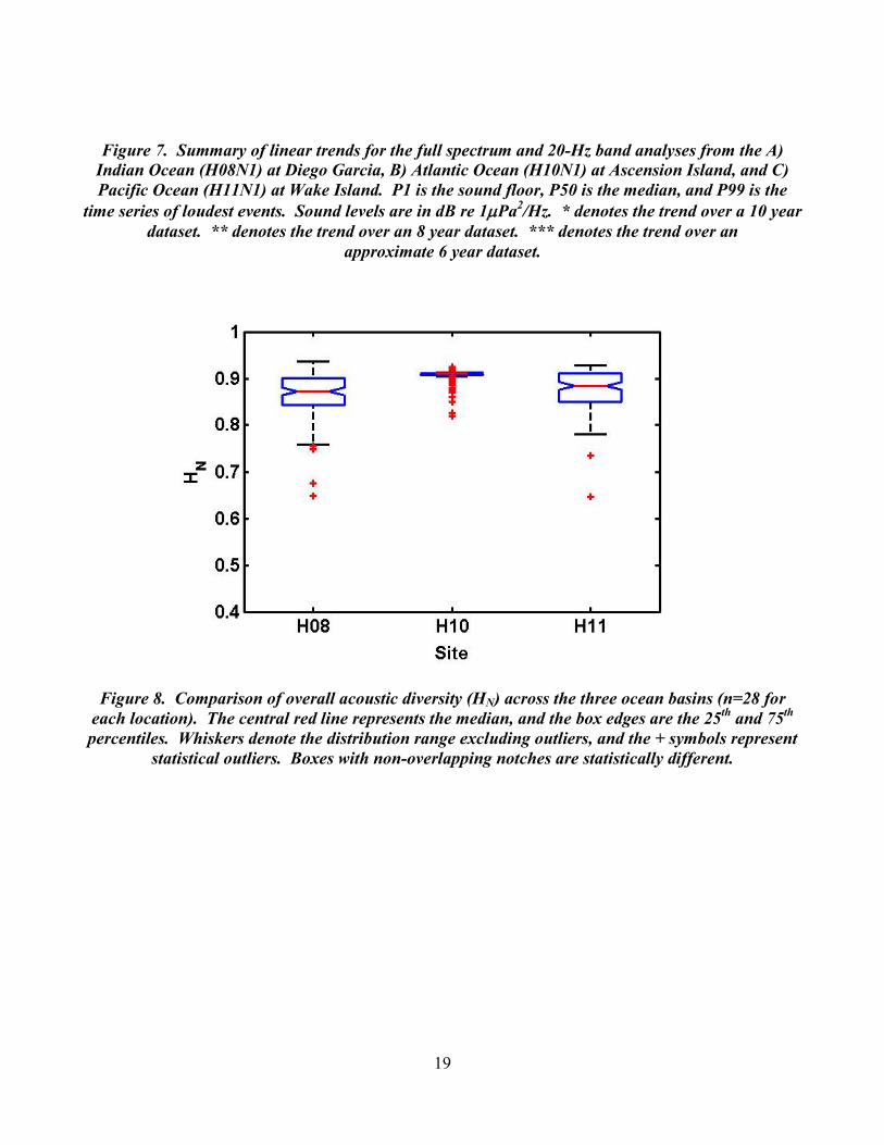
Long term patterns/trends Decomposing the acoustic time series by frequency and sound level afforded the opportunity to examine details of the ambient sound that would not have been observed with traditional descriptive statistics of the full spectrum. Linear regression analyses on the full time series at each location showed no consistent trends across ocean basins, and trends within an ocean were frequency dependent (Figure 7). In the Indian Ocean at Diego Garcia, there has been a consistent increase in the sound floor (P1), but the P99 levels decreased over the past decade. The P50 trend from Diego Garcia showed a strong increase in the 85-105 Hz band, whereas the trend minimally increased for the other 3 frequency categories. In the Atlantic Ocean at Ascension Island, there was an overall decreasing trend for the sound floor in the full spectrum, 40-60 Hz band, and 85-105 Hz band. There was no change in the 10-30 Hz sound floor at this location over the past 8 years. The median (P50) levels over the same time period increased 0.5-1 dB in the full spectrum and 10-30 Hz band while remaining approximately the same in the 40-60 Hz and 85-105 Hz bands. The most extreme levels at Ascension Island showed the greatest difference in the 40-60 Hz band level, most likely associated with an increase in air gun activity (Nieukirk et al., 2012). The extreme sound levels either decreased slightly or remained the same for the other three frequency categories. The Pacific Ocean time series at Wake Island spanned 5.5 years. During this time there was an overall decrease in sound level for the P1 and P50 sound levels. The exception to this overall trend was no change in the 40-60 Hz band for the P50 levels. There was no consistent trend in the P99 levels in the Pacific Ocean at Wake Island. The full spectrum showed the greatest increase, whereas the 40-60 Hz showed the greatest decrease of approximately -1.9 dB. [Full details of the Indian Ocean trends at Diego Garcia can be found in Miksis-Olds et al., in press for Nov 2013 publication in JASA. Summary of the trends in all three oceans at the CTBTO locations was submitted as a book chapter to Springer (Miksis-Olds, 2014).] Assessing biodiversity Acoustic recordings from all three ocean basins contained numerous acoustic signals. Natural seismic activity, including earthquakes and volcanic activity, was detected at all three sites. Acoustic calls from 3 species of baleen whales were detected among the three sites. These include fin whales, blue whales, and sei whales. In the Atlantic (H10), whale calls were detected consistently in the austral summer and not at all in other seasons. Whale calls were detected in all seasons in the Indian Ocean (H08) with the minimum number of fin and blue whale detections occurring in austral summer-fall and winter, respectively. In the Pacific Ocean (H11), the number of detected whale calls peaked in the fall-winter seasons with a minimum in the summer. Ship noise was most prevalent in the Pacific, whereas anthropogenic seismic was detected most often in the Atlantic Ocean (H10). Calculated acoustic entropy (HN) values for six hour time periods for each week long time series at each location indicated that site H10 in the Atlantic Ocean had significantly higher acoustic diversity and greater number of outliers compared to the other two ocean locations (Kruskal-Wallis df=2, Χ2=63.48, p<0.001). The diversity and magnitude of outliers estimated at H08 and H11 were equal (Figure 8). Comparison of the acoustic diversity across seasons at a single location revealed location H10 in the Atlantic Ocean as the most stable over the course of the year. There was no significant difference in acoustic diversity across seasons at H10 (df=3, Χ2=6.11, p=0.11). No whale calls were detected at H10 in three of the four seasons, with detections of blue whale signals only in the austral summer (January) recording. Acoustic diversity measurements at locations H08 and H11 did show differences related to season. In the Indian Ocean (H08), acoustic diversity was significantly higher in fall (April) and spring (October) than in austral summer (January) and winter (June-July) (df=3, Χ2=18.26, p= 0.004). Acoustic diversity measurements at H08 were the lowest in winter, which

7

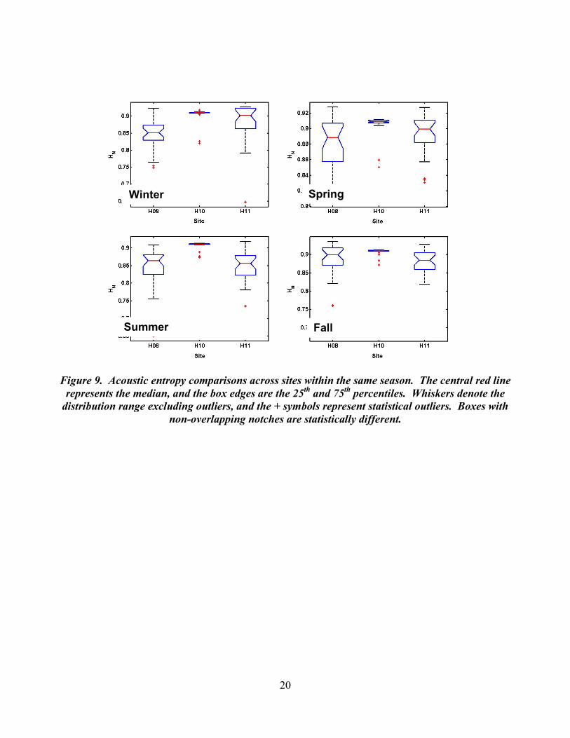
corresponds well to the decrease in the dominant blue whale call counts during this time. Acoustic diversity in the Pacific Ocean was lowest in the summer (July) and highest in the winter (January) and fall (October) which accurately reflects the pattern of whale call counts observed in each season. The final analysis performed was a comparison of acoustic diversity across locations within the same season. During winter and summer, the acoustic entropies were significantly higher at H10 and H11 compared to H08 (winter: df=2, Χ2=26.33, p<0.001, summer: df=2, Χ2=41.27, p< 0.001). There was no statistical difference in the distribution of acoustic entropy between sites H10 and H11 in winter, whereas H10 had a greater acoustic entropy value than H11 in summer (Figure 9). In spring, the acoustic entropy estimates at H10 were significantly higher than at H08 and H11 (df=2, Χ2=8.73, p=0.012). During the fall, the distribution of acoustic entropy estimates at H08 and H10 was similar (df=2, Χ2=9.56, p=0.008). Likewise, the distributions of H08 and H11 were the same (Figure 9). [Full details of the biodiversity assessment can be found in an accepted manuscript at Ecological Informatics (Parks et al., 2013, in press).] IMPACT/APPLICATIONS The unit of analysis effort has shown a significant degree of uncertainty in ambient sound level estimates based on different units of analysis, yet no universally accepted procedure exists for selecting window length or sampling method. The shift in the sound level estimates between comparative ocean ambient sound studies can be substantial if signal processing parameters are not statistically accounted for to confirm interpretation of results and observed trends. The rise in North Pacific ambient sound levels at a rate of 2-3 dB per decade from the 1960’s to the early 2000s has sparked concern about the impact of rising sound levels on the marine environment, but there has been a lack of detailed studies on ambient sound trends in other areas for comparison. The long-term trend work presents results from regions of the Equatorial Pacific, South Atlantic, and Indian Oceans over the past 5-10 years. Parsing the soundscape into frequency categories and sound level percentiles allowed for detailed examination of the acoustic environment that would not have been possible with a single analysis of the full spectrum or with a single sound level parameter. The use of percentiles was valuable in discriminating between trends in the sound floor, median levels, and loudest sound levels. Analysis of the different sound level parameters indicated that a single parameter trend analysis is not sufficient for a comprehensive understanding of sound level dynamics at any one location. Based on the inconsistency of patterns and trends across sound level parameters and frequency at a single location, it is recommended that the soundscape of any region be decomposed into multiple frequency and sound level components to obtain a full understanding of the acoustic dynamics. The preliminary study of biodiversity assessment allowed us to evaluate the feasibility of discriminating levels of bioacoustic signal production both seasonally within a single location and among different sampling stations in three separate ocean basins. The selected dataset, while limited in overall signal bandwidth and species richness, provided a variety of acoustic conditions including recordings that were dominated by human generated sounds, natural abiotic sources, and those dominated by natural biotic signals produced by large baleen whales. With modest signal processing for noise removal, a modified entropy estimate (HN) did provide a potentially useful metric for rapidly assessing the acoustic biodiversity in the marine environment from long-term acoustic recordings though further refinement is necessary.

8

TRANSITIONS This project represents a transition from the acoustic characterization of local and regional areas to the characterization of ocean basins. Detailed knowledge of noise statistics and variation will contribute to reducing error associated with marine animal density estimates generated from passive acoustic datasets, signal detection and localization, and propagation models. RELATED PROJECTS The current project is directly related to and collaborative with ONR Ocean Acoustics Award N00014-11-1-0039 to David Bradley titled “Ambient Noise Analysis from Selected CTBTO Hydroacoustic Sites”. Patterns and trends of ocean sound observed in this study will also be directly applicable to the International Quiet Ocean Experiment being developed by the Scientific Committee on Oceanic Research (SCOR) and the Sloan Foundation (www.iqoe-2011.org). Data being processed and analyzed in this study from the Ascension Island location in the Atlantic continues to be combined with data from Holger Klinck (Oregon State University) to quantify ambient sound across the Atlantic from pole to pole. Data from the Arctic was collected by H. Klinck under Marine Mammal Commission, National Fish and Wildlife Foundation Grant No. 2010-0073-003 and the NOAA Vents Program. Antarctic data was also collected by H. Klinck under a Korea Polar Research Institute award. Sound level analysis of data from the Wake Island location is also to be used in a collaborative study of deep water sound propagation with Michael Ainslie, TNO. Collaborative efforts were joined to better understand the contribution and variation in distant shipping noise to local soundscapes (Ainslie & Miksis-Olds, 2013) REFERENCES Andrew, RK, Howe, BM, Mercer, JA, and MA Dzieciuch. 2002. Ocean ambient sounds: Comparing

the 1960’s with the 1990’s for a receiver off the California coast. ARLO 3: 65-70.

Bendat JS AG Piersol. 2000. Random data: Analysis and measurement procedures/ 3rd edition. Wiley & Sons, New York , NY.

Chapman, NR and A Price. 2011. Low frequency deep ocean ambient noise trend in the Northeast Pacific Ocean. Journal of the Acoustical Society of America 129: EL161-EL165.

Curtis, KR, Howe, BM and JA Mercer. 1999. Low-frequency ambient sound in the North Pacific: Long time series observations. Journal of the Acoustical Society of America 106: 3189-3200.

Hawkins RS. 2013. Variation in low-frequency underwater ambient sound level estimates based on different temporal units of analysis. MS Thesis, The Pennsylvania State University. State College, PA.

Hawkins RS and JL Miksis-Olds. 2103 submitted 7/13. Variation in low-frequency ocean sound estimates based on different temporal units of analysis. Journal of the Acoustical Society of America.

9

Lix, LM, Keselman, JC and HJ Keselman. 1996. Consequences of assumption violations revisited: A quantitative review of alternatives to the one-way analysis of variance F test. Review of Educational Research 66: 579-619.

McDonald, MA, Hildebrand, JA and SM Wiggins. 2006. Increases in deep ocean ambient noise in the Northwest Pacific west of San Nicolas Island, California. Journal of the Acoustical Society of America 120: 711-717.

Mellinger DK and CW Clark. 2000. Recognizing transient low-frequency whale sounds by spectrogram correlation. J. Acoust. Soc. Am.107: 3518-29.

Mellinger DK and CW Clark. 2006. MobySound: A reference archive for studying automatic recognition of marine mammal sounds. Applied Acoustics 67:1226-1242.

Miksis-Olds JL. 2014, accepted. Global trends in ocean noise. The Effects of Sound on Aquatic Life. Springer.

Miksis-Olds JL, Bradley DL, and XM Niu. 2013, in press. Decadal trends in the Indian Ocean ambient sounds. Journal of the Acoustical Society of America.

Nieukirk SL, Mellinger DK, Moore SE, Klinck K, Dziak RP and J Goslin. 2012. Sounds from airguns and fin whales recorded in the mid-Atlantic Ocean, 1999-2009. Journal of the Acoustical Society of America 131: 1102-1112.

Parks SE, Miksis-Olds JL and SL Denes. 2013, in press. Assessing marine ecosystem acoustic diversity across ocean basins. Ecological Informatics.

Ross D. 1993. On ocean underwater ambient noise. Acoustic Bulletin 18: 5-8.

Ross D. 2005. Ship sources of ambient noise. IEEE Journal of Oceanic Engineering 30: 257-261.

Sueur J, Pavoine S, Hamerlynck O and Duvail S. 2008. Rapid acoustic survey for biodiversity appraisal. PLoS ONE, 3: e4065.

Van der Schaar M, Ainslie MA, Robinson SP, Prior MK, and M Andre. 2013 Changes in 63 Hz third-octave band sound levels over 42 months recorded at four deep-ocean observatories. Journal of Marine Systems (in press). Available online 29 July 2013.

Wu Q and B Jeng. 2002. Background subtraction based on logarithmic intensities. Pat. Recog. Let., 23: 1529-1536.

PUBLICATIONS Miksis-Olds JL (2014, accepted). Global trends in ocean noise. The Effects of Sound on Aquatic Life.

Springer.

Hawkins, RS, Miksis-Olds, JL (submitted 7/13). Variation in low-frequency ocean sound estimates based on different temporal units of analysis. Journal of the Acoustical Society of America.

Parks, SE, Miksis-Olds, JL, Denes, SL (2013, in press). Assessing marine ecosystem acoustic diversity across ocean basins. Ecological Informatics.

Miksis-Olds, JL, Bradley, DL, Niu, XM (2013, in press for Nov 2013 publication). Decadal trends in Indian Ocean ambient sound. Journal of the Acoustical Society of America.

10

Miksis-Olds JL (2013). What is an underwater soundscape? In: Proceedings of the 2013 Underwater Acoustics International Conference and Exhibition, Corfu, Greece, June 23-38 2013.

Hawkins, RS (2013). Variation in low-frequency underwater ambient sound level estimates based on different temporal units of analysis. MS Thesis, The Pennsylvania State University. State College, PA.

Miksis-Olds JL, Smith CM, Hawkins RS and Bradley DL (2012). Seasonal soundscapes from three ocean basins: what is driving the differences? Conference Proceedings of the 11th European Conference on Underwater Acoustics 34: 1583- 1587. ISBN 978-1-906913-13-7.

Hawkins RS, Miksis-Olds JL, Bradley DL and Smith CM (2012). Periodicity in ambient noise and variation based on different temporal units of analysis. Conference Proceedings of the 11th European Conference on Underwater Acoustics 34: 1417- 1423. ISBN 978-1-906913-13-7. (First author is student of Miksis-Olds)

Nichols SM, Bradley DL, Miksis-Olds JL and Smith CM (2012). Are the world’s oceans really that different? Conference Proceedings of the 11th European Conference on Underwater Acoustics 34: 338- 345. ISBN 978-1-906913-13-7.

PRESENTATIONS Ainslie, MA, Miksis-Olds, JL (2013). Periodic changes in deep ocean shipping noise: Possible causes

and their implications. Bioacoustics Day, Leiden, Netherlands, September 18, 2013.

Miksis-Olds JL (2013). Global trends in ocean noise. The Effects of Sound on Aquatic Animals, Budapest, Hungary, August 12-16, 2013.

Miksis-Olds JL (2013). What is an underwater soundscape? 2013 Underwater Acoustics International Conference and Exhibition, Corfu, Greece, June 23-38 2013.

HONORS/AWARDS/PRIZES Office of Naval Research Young Investigator Program (YIP) Award – 2011

11

Table 1. Acoustic sensor location summary. Latitude areas in parentheses under Latitude Region indicate acoustic focus of sensors on opposite sides of island.

Site Element Acoustic Focus System Location

Latitude Region of

Sensor

Major Oceanogrphic

Process

HA08 N Equatorial Indian CTBTO Diego Garcia,

UK Low Equatorial Current

S Indian CTBTO Diego Garcia, UK

Low (Mid)

Equatorial Current

HA11 N W Pacific CTBTO Wake Is., USA Low (Mid)

N Equatorial Current

S Equatorial Pacific CTBTO Wake Is., USA Low N Equatorial

Current

HA10 N Equatorial Atlantic CTBTO Ascension Is.,

UK Low S Equatorial Current

S S Atlantic CTBTO Ascension Is., UK

Low (Mid)

S Equatorial Current

Table 2. Data successfully downloaded and available to ARL Penn State.

Site/Location Start Day Most Recent Download

# Missing Days Total Days Total Years

HA08/Diego Garcia

01/21/2002 06/13/2013 40 4122 11.3

HA10/Ascension Island

11/04/2004 06/13/2013 4 3140 8.6

HA11/Wake Island

04/25/2007 06/13/2013 14 2227 6.1

Figure 1. Location of CTBTO Hydroacoustic Sites. H sites denote hydrophone sites, moored in the water column at sound channel depths. T sites denote seismic “T-phase” sensors. This project will

use data from H08, H10, and H11.

12

Figure 2. a) H values and the related number of whale calls for 1-2 Jan 2008 from H08N in the Indian Ocean. b) HN values and related number of whale calls. Note the HN values increase with

increased numbers of whale calls, while H shows no relationship with biological signal levels.

a) b)

13

a)

b)

:E 10

J: 15

~ .! 30

~ "C 60 c: :!: 200

7.3

North

----&--

~J

7.4 7.5 7.6 7.7 7.8

Mean Rank x 104

0.4 ,....-----.------.---.....------,

0.3

>---~ 0.2 Q)

c 0.1

--Window= 10s --Window= 15s --Window = 30s --Window= 60s --Window= 200s

South

:E 10 ----&--

J: 15 j c, c: .! 30

~ 60 "C c: :!: 200

7.3 7.4 7 .5 7.6 7.7 7.8

Mean Rank X 104

0.3....------~----------,

0.25

>- 0.2 -·~ 0.15 Q)

c 0.1

0.05

0~-d~~----~~~ .. --~ 90 95 100 105 85 90 95 100 105

:E 10 J: c, 15 c:

..9:! 30

~ "C

60 c: ~ 200

0.3

0.25

~ 0.2 'ij) s::: 0.15 ~

0.1

0.05

Sound Level (dB re 1,_.Pa2/Hz)

North

-€-

E1t-c 7.5 a a.5

Mean Rank

0~~~--~~~----------~ 75 80 85 90 95 100

Sound Level (dB re 1JJPa2/Hz)

~ 10 .s::: .... C) 15 s::: ~ 30

~ 60 "C s::: :: 200

0.25

~ 0.2 Iii s::: 0.15 Ql

c 0.1

0.05

Sound Level (dB re 1,_.Pa2/Hz)

South

-e-

E~~ 7.5 8 8.5

Mean Rank

--Window = 10s --Window = 15s --Window = 30s --Window = 60s --Window = 200s

75 80 85 90 Q5 100

Sound Level (dB re 1JtPa2/Hz)

14

Figure 3. Example of multiple comparison and probability density plots from H08N1 (left) and of H08S2 (right) over 5 window lengths from 1-week period 01-08 Oct 2008. A): full spectrum, B): 10-30 Hz band, C): 40-60 Hz band, D): 85-105 Hz band. Arrows indicate location of 95% significant

difference color coded by pair.

c)

d)

15

Figure 4. Example of multiple comparison and probability density plots from H08N1 (left)

and of H08S2 (right) over 5 subsample rates from 6-week period 01 Jan 2005 to 12 Feb 2005. A) shows full spectrum results for the 60 s window length analysis at subsampling intervals of 1, 5, 10,

30, and 60 min. B) shows full spectrum results for the 200 s window length analysis for subsampling intervals of 3.3, 10, 16.6, 33.3, and 50 min. Arrows indicate location

of 95% significant difference color coded by pair.

a)

b)

16

Figure 5. Proportion of significant/non-significant results from 100 randomized Kruskal-Wallis tests in each frequency category for the 60 s and 200 s window length analyses. The bar graph is organized into groups by frequency category, and each group contains both window size (60s and

200s) analyses over 5 subsampling intervals The 60s analysis tested 1, 5, 10, 30, and 60 s subsampling intervals. The 200 s analysis tested 3.3, 10, 16.6, 33.3 and 50 min subsampling

intervals. Significance of the observed proportions at a 95% significance level was tabulated via a normalized cumulative probability density function.

5-110 Hz

17

Figure 6. Maximum differences between highest and lowest 6-week sound level estimates across subsampling interval (n=100) for the 60 s (top) and 200 s (bottom) window length analyses. The

median is designated by the horizontal red line with the 25th and 75th percentiles bounding the blue box. Red (+) symbols indicate outliers and are shown to demonstrate overall variation, while the

whiskers indicate the range of data points not considered outliers.

5-110 Hz 5-110 Hz

18

A) Indian Ocean (H08)*

B) Atlantic Ocean (H10)**

C) Pacific Ocean (H11)***

2/04 11/06 8/09 5/12 2/04 11/06 8/09 5/12

Soun

d Le

vel

-1

.0

0

1

.0

Soun

d Le

vel

-1

.0

0

1

.0

-1.0

0

1.0

-1.0

0

1.0

Soun

d Le

vel

-0

.5

0

0.

5

Soun

d Le

vel

-0

.5

0

0.5

-0

.5

0

0.

5

-0.5

0

0

.5

7/05 11/06 4/08 8/09 12/10 5/12 7/05 11/06 4/08 8/09 12/10 5/12

Soun

d Le

vel

-1

.0

0

1.0

Soun

d Le

vel

-1

.0

0

1.0

-1.0

0

1.

0

-1.0

0

1.

0

4/08 8/09 12/10 5/12 4/08 8/09 12/10 5/12

19

Figure 7. Summary of linear trends for the full spectrum and 20-Hz band analyses from the A) Indian Ocean (H08N1) at Diego Garcia, B) Atlantic Ocean (H10N1) at Ascension Island, and C) Pacific Ocean (H11N1) at Wake Island. P1 is the sound floor, P50 is the median, and P99 is the

time series of loudest events. Sound levels are in dB re 1µPa2/Hz. * denotes the trend over a 10 year dataset. ** denotes the trend over an 8 year dataset. *** denotes the trend over an

approximate 6 year dataset.

Figure 8. Comparison of overall acoustic diversity (HN) across the three ocean basins (n=28 for each location). The central red line represents the median, and the box edges are the 25th and 75th percentiles. Whiskers denote the distribution range excluding outliers, and the + symbols represent

statistical outliers. Boxes with non-overlapping notches are statistically different.

20

Figure 9. Acoustic entropy comparisons across sites within the same season. The central red line represents the median, and the box edges are the 25th and 75th percentiles. Whiskers denote the

distribution range excluding outliers, and the + symbols represent statistical outliers. Boxes with non-overlapping notches are statistically different.

Winter Spring

Summer Fall