ocean conditions and salmon survival in the northern ... · 2032 s marine science drive newport,...

Ocean Conditions and Salmon Survival in the Northern California Current

William T. Peterson,1 Rian C. Hooff,2 Cheryl A. Morgan,3 Karen L. Hunter,3

Edmundo Casillas,1 and John W. Ferguson1

1Fish Ecology Division Northwest Fisheries Science Center National Marine Fisheries Service

Newport Research Station 2032 S Marine Science Drive Newport, Oregon 97365-5275

2Aquatic Ecology Lab Department of Biological and Environmental Sciences

Washington State University, Vancouver

3Cooperative Institute for Marine Resource Studies Hatfield Marine Science Center

Oregon State University 2030 S Marine Science Drive

Newport, Oregon 97365

November 2006

EXECUTIVE SUMMARY

Over the past three decades, physical and biological oceanographic conditions have varied greatly in continental shelf waters of the northern California Current (CC) off the Pacific Northwest. Between 1977 and 1998, the northern CC was in a warm and relatively unproductive phase; as a result, salmon numbers in the Pacific Northwest declined significantly. Two of the largest tropical El Niño events of the century occurred during these 22 years: one in 1983 and a second during 1997-1998. These remote events contributed to exceptionally warm ocean temperatures in the northern CC.

During the past 10 years, conditions in the northern CC have been particularly variable, with the 1997-1998 El Niño followed by 4 years of tropical La Niña events, which contributed to a period of cool and productive ocean conditions. During this period, Pacific Northwest salmon numbers rebounded dramatically. However, in late 2002, oceanographic conditions again reversed, and warm conditions prevailed for the next four years. This recent return to a warm phase coincided with a decline in adult return rates of both coho and yearling Chinook salmon, reversing the trend of high adult returns observed from 2000 to 2003.

As many scientists and salmon managers have noted, variations in marine survival of both coho and Chinook salmon correspond with periods of alternating cold and warm ocean conditions. Cold conditions are generally good for Chinook and coho salmon, whereas warm conditions are not. Our research is focused on identifying the ecological linkages that accompany warm vs. cold ocean conditions, and on how changes in ocean conditions affect salmon survival.

This report provides an overview of these topics for the non-specialist. We include a discussion of basic oceanography and of the interactions between physical and biological ocean processes as appendices. Three sets of ecosystem indicators are presented to aid in understanding the ecological interactions presented here and for use in predicting adult salmon returns. The first set is based on large-scale oceanic and atmospheric conditions in the North Pacific Ocean, and consists of the Pacific Decadal Oscillation and the Multivariate El Niño Southern Oscillation Index. These metrics help gauge the influence of basin-scale winds and ocean currents on local ocean dynamics off the Pacific Northwest.

The second set of indicators is based on local observations of physical and biological ocean conditions off Newport, Oregon. These observations were recorded during oceanographic research cruises by NOAA Fisheries scientists since 1996. They

iii

include measures of upwelling, water temperature and salinity characteristics, and plankton species compositions, among other elements. The third set of indicators is based on biological sampling of plankton, juvenile salmonids, forage fish, and Pacific hake. These indices were developed from recorded observations of biological conditions in coastal waters off Oregon and Washington since 1998. Additional indicators are being developed or considered for development, and their status is discussed as well.

From this combination of physical and biological indicators, we attempt to produce forecasts of adult salmon returns. At this time, these forecasts are qualitative in nature, in that we rate each indicator in terms of “good,” “bad,” or “neutral,” based on its relative impact on marine survival of juvenile salmon. Two caveats to these forecasts should be noted: first, relative forecast indicators must be viewed within a historical context. That is, a “good” forecast for coho or spring Chinook is made relative to returns observed over the past 10 years. Second, at this time forecasts are focused on hatchery coho salmon. Columbia River spring Chinook are discussed, but data for the species was not divided by stock. In future years we plan to compare and contrast hatchery vs. wild coho, as well as the different Chinook stocks, including subyearling Chinook. In Table 1, we summarize all of the indices discussed here and present a simple color system that codes the qualitative influence of each indicator.

As shown in Table 1, almost all ecosystem indices measured in 2005 point to low adult returns of hatchery coho salmon in 2006 and spring Chinook salmon in 2007. From late 2002 through 2005, the PDO has been positive, and coastal ocean temperatures have remained 1-2°C above normal. Both of these indicators signal unfavorable ocean conditions for these two salmon species.

In addition, the spring transition date was very late (i.e., strong and sustained upwelling did not start until mid-July) and copepod species diversity was high. Also in 2005, a large negative anomaly in the northern (cold water) copepod biomass occurred. This anomaly was nearly as large as the largest yet recorded, which occurred during the 1998 El Niño. Moreover, we collected the fewest numbers of juvenile salmon during June and September 2005 than during any of our previous trawl surveys, even those conducted during the 1998 El Niño. Thus, nearly all indicators suggest smolt-to-adult returns rates of no more than 1% for both coho salmon in 2006 and spring Chinook salmon in 2007.

iv

Table 1. Ocean and ecosystem conditions in the Northern California Current. Colored dots indicate whether the index was positive (green), neutral (yellow), or negative in the year salmon entered the ocean. The last two columns forecast adult returns based on ocean conditions in 2005. We include the year 2000 as an example of conditions during a "good" year, in contrast to the "poor" conditions observed in recent years, 2004-2006.

Juvenile migration year Forecast of adult returns

Coho Chinook 2000 2004 2005 2006 2006 2007

Large-scale ocean and atmospheric indicators

PDO ■ ■ ■ ■ ● ● MEI ■ ■ ■ ■ ● ● Local and regional physical indicators

Sea surface temperature ■ ■ ■ ■ ● ● Coastal upwelling ■ ■ ■ ■ ● ● Physical spring transition ■ ■ ■ ■ ● ● Deep water temp. & salinity ■ ■ ■ ■ Local biological indicators

Copepod biodiversity ■ ■ ■ ■ ● ● Northern copepod anomalies ■ ■ ■ ■ ● ● Biological spring transition ■ ■ ■ ■ ● ● Spring Chinook--June ■ ■ ■ ■ ● ● Coho--September ■ ■ ■ ■ ● ●

Key ■ good conditions for salmon marine survival ● good returns expected ■ intermediate conditions for salmon marine survival ■ poor conditions for salmon marine survival ● poor returns expected

v

CONTENTS

EXECUTIVE SUMMARY ............................................................................................... iii

INTRODUCTION .............................................................................................................. 1

LARGE-SCALE OCEAN AND ATMOSPHERIC INDICATORS .................................. 3 Pacific Decadal Oscillation (PDO) ......................................................................... 3 Multivariate El Niño Southern Oscillation Index (MEI) ........................................ 5

LOCAL AND REGIONAL PHYSICAL INDICATORS .................................................. 7 Sea Surface Temperature Anomalies...................................................................... 7 Coastal Upwelling Index (CUI) .............................................................................. 9 Spring Transition in Physical Oceanographic Conditions .................................... 11 Deep-Water Temperature and Salinity ................................................................. 13

LOCAL BIOLOGICAL INDICATORS........................................................................... 17 Copepod Biodiversity ........................................................................................... 17 Northern and Southern Copepod Anomalies ........................................................ 19 The Biological Spring Transition.......................................................................... 22 Catches of Spring Chinook and Coho Salmon during June and September Trawl Surveys.................................................................................................................. 23

INDICATORS UNDER DEVELOPMENT..................................................................... 25 A Second Mode of North Pacific Sea Surface Temperature Variation ................ 25 Phytoplankton Biomass ........................................................................................ 25 Interannual Variations in Habitat Area ................................................................. 26 Copepod Community Structure ............................................................................ 26 Forage Fish and Pacific Hake Abundance ............................................................ 26 Salmon Predation Index........................................................................................ 28 Potential Indices for Future Development ............................................................ 28

FORECAST of COHO and CHINOOK ADULT RETURNS in 2006 and 2007............. 29

REFERENCES ................................................................................................................. 31

APPENDIX A: Introduction to the Local Oceanography................................................ 33

APPENDIX B: At-Sea Sampling Methods...................................................................... 39

APPENDIX C: Web Sites for Addtional Information..................................................... 44

vii

INTRODUCTION

This report describes how physical and biological oceanographic conditions may affect the growth and survival of juvenile salmon in the northern California Current off Oregon and Washington. We present a number of physical, biological, and ecosystem metrics that specifically define the term “ocean conditions.” More importantly, these metrics can be used to forecast the survival of salmon 1-2 years in advance. Most of the information is based on our own (NOAA Fisheries) observations during frequent oceanographic cruises made since 1996 to study the coastal upwelling ecosystem off the Pacific Northwest.

Using information derived from more than 10 years of physical and biological ocean observations, we developed environmental indicators to provide ecosystem-based forecasts of salmon returns. These forecasts are presented as a practical example of how ocean ecosystem indicators can be used to inform management decisions for endangered salmon.

These ocean indicators compliment three existing physical indicators that can be used to predict adult salmon runs: (1) jack salmon returns, (2) the Logerwell et al. (2003) index of coho salmon returns and (3) Scheuerell and Williams (2005) index of Snake River Chinook salmon returns. The latter two methods are based on the strength of upwelling, sea surface temperature, and sea level. Each of these indicators has shown utility in predicting adult salmon returns. However components of each, such as upwelling, have at times proven to be poor indicators.

To improve forecasting of salmon returns, we utilize a suite of indicators, based on measurements of both physical and biological oceanographic conditions. The strength of this approach is that biological indicators are directly linked to the success of salmon during their first year at sea through food chain processes. These biological indicators, coupled with physical oceanographic data, offer new insight into the mechanisms that lead to success or failure for salmon runs.

In addition to forecasting salmon returns, the indicators presented here may be of use to those trying to understand how variations in ocean conditions might affect recruitment of fish stocks, seabirds, and other marine animals. We reiterate that trends in salmon survival track regime shifts in the North Pacific Ocean, and that these shifts are transmitted up the food chain in a more-or-less linear and bottom-up fashion as follows:

upwellingÆ nutrients Æ plankton Æ forage fish Æ salmon.

___________________________________________

La Push

Queets River

Grays Harbor

Willapa Bay

Columbia River

Cape Meares

Cascade Head

^

Cape Falcon

Cape Perpetua

Newport

Washington

Oregon

The same regime shifts that affect Pacific salmon also affect the migration of Pacific hake and the abundance of sea birds, both of which prey on migrating juvenile salmon. Therefore, climate variability can also have “top down” impacts on salmon through predation by hake and sea birds (terns and murres). Both “bottom up” and “top down” linkages are explored here.

Data used here are from several sources. First, the in situ ocean observations, most of which resulted from the more than 250 oceanographic cruises conducted by NOAA Fisheries from 1996 to 2006 in the coastal waters off Newport, Oregon.

These are combined with earlier observations made off Newport during 1969-1973, 1983, and 1991-1992.

Second, we include results of measurements collected during broad-scale surveys of ocean conditions and juvenile salmon abundance in the continental shelf waters off Oregon and Washington. These surveys were conducted each June and September from 1998 to present. The sampling grid established from these surveys is shown in Figure 1. Finally, we incorporate data from websites reporting on the Pacific Decadal Oscillation (PDO) and El Niño Southern Oscillation (ENSO), as well as date from NOAA weather126° W 125° W 124° W 123° W126° W 125° W 124° W 123° Wbuoys.1

Figure 1. Transects sampled during trawling surveys off the coast of Oregon and Washington.

1 Readers of this report may be interested in a similar document produced annually by marine scientists from the Pacific Region of Canada’s Fisheries and Ocean group on Vancouver Island: http://www-sci.pac.dfo-mpo.gc.ca/psarc/OSRs/Ocean_SSR_e.htm.

45° N

46° N

47° N

48° N

_

45° N

46° N

47° N

48° NLa Push

Queets River

Grays Harbor

Willapa Bay

Columbia River

Cape Meares

Cascade Head

_̂

Cape Falcon

Cape Perpetua

Newport

Washington

Oregon

2

http://www-sci.pac.dfo-mpo.gc.ca/psarc/OSRs/Ocean_SSR_e.htm

LARGE-SCALE OCEAN AND ATMOSPHERIC INDICATORS

Pacific Decadal Oscillation (PDO)

The Pacific Decadal Oscillation is a climate index based upon patterns of variation in sea surface temperature of the North Pacific from 1900 to the present (Mantua et al. 1997). While derived from sea surface temperature data, the PDO index is well correlated with many records of North Pacific and Pacific Northwest climate and ecology, including sea level pressure, winter land-surface temperature and precipitation, and stream flow. The index is also correlated with salmon landings from Alaska, Washington, Oregon, and California.

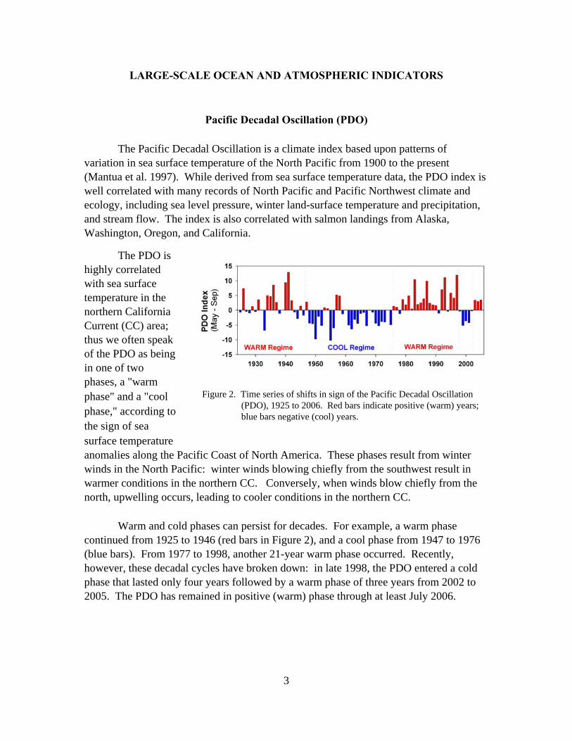
The PDO is highly correlated with sea surface temperature in the northern California Current (CC) area; thus we often speak of the PDO as being in one of two phases, a "warm phase" and a "cool phase," according to the sign of sea surface temperature anomalies along the Pacific Coast of North America. These phases result from winter winds in the North Pacific: winter winds blowing chiefly from the southwest result in warmer conditions in the northern CC. Conversely, when winds blow chiefly from the north, upwelling occurs, leading to cooler conditions in the northern CC.

Warm and cold phases can persist for decades. For example, a warm phase continued from 1925 to 1946 (red bars in Figure 2), and a cool phase from 1947 to 1976 (blue bars). From 1977 to 1998, another 21-year warm phase occurred. Recently, however, these decadal cycles have broken down: in late 1998, the PDO entered a cold phase that lasted only four years followed by a warm phase of three years from 2002 to 2005. The PDO has remained in positive (warm) phase through at least July 2006.

Figure 2. Time series of shifts in sign of the Pacific Decadal Oscillation (PDO), 1925 to 2006. Red bars indicate positive (warm) years; blue bars negative (cool) years.

3

Dr. Nathan Mantua and his colleagues were the first to show that adult salmon catches in the Northeast Pacific were correlated with the Pacific Decadal Oscillation (Mantua et al. 1997). They noted that in the Pacific Northwest, the cool PDO years of 1947-1976 coincided with high returns of Chinook and coho salmon to Oregon rivers. Conversely, during the warm PDO cycle that followed (1977-1998), salmon numbers declined steadily.

The listing of several salmon stocks as threatened or endangered under the U.S. Endangered Species Act coincides with a prolonged period of poor ocean conditions

that began in the early 1990s. This is illustrated in Figure 2, which shows average PDO values in summer vs. anomalies in counts of adult spring Chinook at Bonneville Dam. Also shown are percentages of hatchery juvenile coho salmon that returned as adults to hatcheries in SW Washington and NE Oregon during this period. These percentages have been recorded since 1961 as the Oregon Production Index, Hatchery (OPIH).

The OPIH includes fish taken the fishery as well as those that returned to hatcheries. Figure 3 shows a clear visual correlation between the PDO, adult spring Chinook counts and hatchery coho adult returns note that during the 22-year cool phase of the PDO (1955 to 1977), below-average counts of spring Chinook at Bonneville Dam were seen in only 5 years (1956, 1958-60, and 1965).

In contrast, below-average counts were common from 1977 to 1998, when the PDO was in warm phase: below-average counts were observed in 16 of these 21 years. The dramatic increase in counts from 2000 to 2004 coincided with the return to a cool phase PDO in late 1998. Note also from Figure 3 that a time lag of up to 2 years exists between PDO phase changes and spring Chinook returns: Chinook runs remained above average in 1977 and 1978, 2 years after the 1976 PDO shift. Similarly, increased returns of spring Chinook adults in 2000 lagged 2 years behind the PDO shift of 1998.

Figure 3. Summer average PDO (top) vs. adult spring Chinook passing Bonneville Dam (middle) and survival of hatchery coho salmon (bottom), 19552006. Vertical lines indicate climate-shift points in 1977 and 1998.

4

_________________________________

Multivariate El Niño Southern Oscillation Index (MEI)

Coastal waters off the Pacific Northwest are influenced by atmospheric conditions not only in the North Pacific Ocean (as indexed by the PDO), but also in equatorial waters, especially during El Niño events. Strong El Niño events result in the transport of warm equatorial waters northward along the coasts of Central America, Mexico, and California and into the coastal waters off Oregon and Washington. Thus, these events affect weather in the Pacific Northwest, often resulting in stronger winter storms and transport of warm, offshore waters into the coastal zone. The transport of warm waters toward the coast, either from the south or from offshore, also results in the presence of unusual mixes of zooplankton and fish species.

El Niño events have variable and unpredictable effects on coastal waters off Oregon and Washington. While we do not fully understand how El Niño signals are transmitted northward from the equator, we do know that signals can travel through the ocean via Kelvin waves.2 Kelvin waves propagate northward along the coast of North America and result in transport of warm waters from south to north.

El Niño signals can also be transmitted through atmospheric teleconnections,3 in that El Niño conditions can strengthen the Aleutian Low, a persistent low-pressure air mass over the Gulf of Alaska. Thus adjustments in the strength and location of low-pressure atmospheric cells at the equator can affect our local weather, resulting in more frequent large storms in winter and possible disruption of upwelling winds in spring and summer.

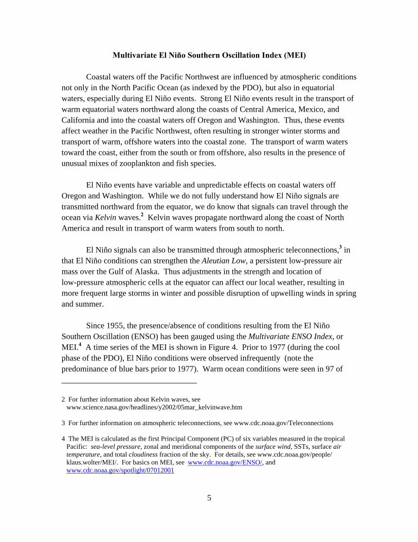
Since 1955, the presence/absence of conditions resulting from the El Niño Southern Oscillation (ENSO) has been gauged using the Multivariate ENSO Index, or MEI.4 A time series of the MEI is shown in Figure 4. Prior to 1977 (during the cool phase of the PDO), El Niño conditions were observed infrequently (note the predominance of blue bars prior to 1977). Warm ocean conditions were seen in 97 of

2 For further information about Kelvin waves, see www.science.nasa.gov/headlines/y2002/05mar_kelvinwave.htm

3 For further information on atmospheric teleconnections, see www.cdc.noaa.gov/Teleconnections

4 The MEI is calculated as the first Principal Component (PC) of six variables measured in the tropical Pacific: sea-level pressure, zonal and meridional components of the surface wind, SSTs, surface air temperature, and total cloudiness fraction of the sky. For details, see www.cdc.noaa.gov/people/ klaus.wolter/MEI/. For basics on MEI, see www.cdc.noaa.gov/ENSO/, and www.cdc.noaa.gov/spotlight/07012001

5

the 269 months from 1955 to 1976, with moderate-to-strong El Niño events observed in 1957-1958, 1966, 1969, and 1972.

In contrast, the warm phase of the PDO from 1976 to 1998 was characterized by nearly continuous favorable ENSO conditions. During these 22 years,cool conditions were observed in only 98 of 266 months.

Figure 4. The MEI from 1955 to 2006. Vertical lines delineate climate shifts in 1976, 1998, and 2002. Red bars indicate El Niño conditions. Note the +3 anomaly associated with the 1983 and 1998 events, and the prolonged “weak event” from 1989 to 1996. Note also the return to negative (cool) anomalies in 2005. Vertical lines delineate years in which the PDO changed phase (1977, 1998, 2002)

During this same warm phase of the PDO, both the equatorial and northern North Pacific oceans experienced two very large El Niño events (1983-1984 and 1997-1998). There were also two smaller events in 1986 and 1987 and a prolonged event from 1990 to 1995. Beginning in September 1998, MEI values turned negative and remained so for nearly four years, similar to the trend observed in the PDO. The MEI returned to positive in April 2002 and remained so through September 2005, after which negative values returned.

Both the PDO and MEI can be viewed as “leading indicators,” since after a persistent change in sign of either index, ocean conditions in the California Current soon begin to change. Most recently, the MEI (September 2005) appears to have signaled a return to cold ocean conditions in the Pacific Northwest, as is being observed during the summer of 2006. However, if the positive sign persists, warm conditions can be expected in the future.

The impact of El Niño events on survival of coho salmon is well documented (Pearcy 1992). For example, the large events of both 1983 and 1998 were followed by low adult return rates for coho salmon during 1983-1984 and 1999, respectively. Likewise, the extended period of El Niño conditions in 1977-1983 was accompanied by declines in adult coho returns during the same years. A second extended El Niño period during 1990-1996 was followed by extremely low returns of adult fish that migrated to sea as juveniles from 1991 to 1998. For spring Chinook, the two large (but brief) El Niño events resulted in lower than average smolt-to-adult return rates, but the lowest adult return rates were observed during the weaker but prolonged El Niño events of 1990-1998.

6

LOCAL AND REGIONAL PHYSICAL INDICATORS

Sea Surface Temperature Anomalies

Given that the Pacific Decadal Oscillation is a basin-scale index of North Pacific sea surface temperatures (SST), how closely does the PDO match local sea surface temperatures off the Pacific Northwest? We examined this using data from NOAA Weather Buoy 46050, located 22 miles off Newport, Oregon.

Figure 5 shows monthly PDO values vs. monthly average sea surface temperatures at NOAA Weather Buoy 46050 from 1996 to 2006. This is the period during which we have been measuring ocean conditions off the coast of Oregon.

Correspondence between the PDO and local temperature anomalies is very high. For example, the four years of negative PDO values from late 1998 until late 2002 closely match the negative SST anomalies measured off Newport. Timing of the positive PDO values also matches that of the positive SST anomalies.

This suggests that changes in basin-scale forcing result in local SST changes, and that local changes may be due to differences in transport of water out of the North Pacific into the northern California Current. The data also verify that we can often use local SST as a proxy for the PDO. However, there are periods in which local and regional changes in the northern CC may diverge from the basin-scale PDO pattern for short periods (usually less than a few months).

Figure 5. The PDO and monthly sea surface temperature anomalies at NOAA Buoy 46050, 22 miles west of Newport OR. Data gaps in the records resulted from damage to the buoy by winter storms.

7

Buoy temperatures clearly identify warm and cold ocean conditions. During the 1997-1998 El Niño event, summer water temperatures were 1-2°C above normal, whereas during 1999-2002, they were 2°C cooler than normal. The summers of 2003-2005 were again warm, and some months showed positive SST anomalies that exceeded even those seen during the 1998 El Niño event. Some marine scientists refer to 2003-2005 as having “El Niño-like” conditions.

Note also in Figure 5 that there are time lags between a change in sign of the PDO and change in SST off Newport. In 1998, the PDO changed to negative in July, and SSTs changed to negative in December. In 2002, the opposite pattern was seen, with the PDO change in August followed by SSTs in December. Thus, it takes 5-6 months for the signal in the North Pacific to propagate to coastal waters.

Figure 5 demonstrates that basin-scale indicators such as the Pacific Decadal Oscillation (PDO) do manifest themselves locally: local SSTs change in response to physical shifting on a North Pacific basin scale. Other local changes associated with basin-scale indicators include the source waters that feed into the northern California Current, zooplankton and forage-fish community types, and abundance of salmon predators such as hake and sea birds. Thus, local variables change in response to change that occurs on a broad spectrum of spatial scales. These range from basin-scale changes, which are indexed chiefly by the PDO, to local and regional changes, such as those related to shifts in the jet stream, atmospheric pressure, and surface wind patterns.

8

____________________________________

Coastal Upwelling Index (CUI)

Perhaps the most important process affecting plankton production off the Pacific Northwest is coastal upwelling. Upwelling is caused by northerly winds that dominate from April to September along the Oregon coast. These winds transport offshore surface water southward (yellow arrow in Figure 6), with a component transported away from the coastline (to the right of the wind, light blue arrow). This offshore, southward transport of surface waters is balanced by onshore northward transport of cool, high-salinity, nutrient-rich water (blue arrow).

The strength of an upwelling process can be calculated based on estimates of wind speed. Using such data, Dr. Andy Bakun developed the Coastal Upwelling Index (Bakun 1973).5

Figure 6. Forces affecting coastal upwelling. Drawing courtesy of Environmental Research Division, Pacific Fisheries Environmental Research Laboratory, NOAA.

The CUI is, as its name implies, a measure of the volume of water that upwells along the coast; it identifies the amount of offshore transport of surface waters due to geostrophic wind fields. These wind fields are calculated from surface atmospheric pressure fields measured and reported provided by the U.S. Navy.6 The CUI is calculated in 3-degree intervals from 21°N to 60°N latitude, and

data is available from 1947 to present. For the northern California Current, relevant values are from 42, 45, and 48°N. Year-to-year variations in upwelling off Newport (45°N) are shown as CUI anomalies in Figure 7. The years of strongest upwelling were

Figure 7. Anomaly of the Coastal Upwelling Index from 1947 to 2006, averaged for May-September.

5 Further information on the CUI and a listing of daily and monthly values are available at: http://www.pfel.noaa.gov/products/PFEL/modeled/indices/PFELindices.html.

6 Data available from U.S. Navy Fleet Numerical Meteorological and Oceanographic Center (FNMOC) in Monterey, CA: www.fnmoc.navy.mil/

9

http://www.pfel.noaa.gov/products/PFEL/modeled/indices/PFELindices.html

Figure 8. Scattergram of coho survival vs. CUI anomaly for 45°N, 1960-2004. Panel A shows values during April; panel B shows values during April and May. combined

1965-1967. Upwelling was anomalously weak in all but 8 of the 21 years from summer 1976 to summer 1997, and this is expected during warm PDO phases. When the PDO was in a cool phase (late 1998-2003), upwelling strengthened. With the change in PDO sign to positive in 2004-2005, upwelling again weakened.

Many studies have shown correlations between the amount of coastal upwelling and production of various fisheries. The first to show a predictable relationship between coho survival and upwelling were Gunsolus (1978) and Nickelson (1986).

Knowledge of upwelling alone does not always provide good predictions of salmon returns. For example, during the 1998 El Niño event, upwelling was relatively strong, as measured by the CUI; however, plankton production was weak. This occurred because the deep-source waters for upwelling were warm and nutrient-poor. Low levels of plankton production may have impacted all trophic levels up the food chain. This observation demonstrates the importance of interpreting the upwelling index in light of the type of source water that upwells in the northern California Current.

The relationship between coho salmon survival and upwelling is shown in Figure 8. The strongest correlations with survival were found with upwelling in April and upwelling in April and May combined. A significant, but weaker correlation was also found between upwelling and survival during the months of April, May, and June combined.

Using regression analysis and the value of the upwelling anomaly for April 2006 (which was -9), the 95% confidence intervals suggest a return of coho salmon between 2.8 and 4.5% in 2007. Scheuerell and Williams (2005) showed that the upwelling index in April, September, and October is also related to returns of Snake River spring Chinook salmon. Moreover, they developed a one-year forecast of spring Chinook returns using the CUI.

10

Spring Transition in Physical Oceanographic Conditions

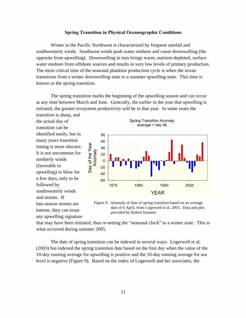
Winter in the Pacific Northwest is characterized by frequent rainfall and southwesterly winds. Southwest winds push water onshore and cause downwelling (the opposite from upwelling). Downwelling in turn brings warm, nutrient-depleted, surface water onshore from offshore sources and results in very low levels of primary production. The most critical time of the seasonal plankton production cycle is when the ocean transitions from a winter downwelling state to a summer upwelling state. This time is known as the spring transition.

The spring transition marks the beginning of the upwelling season and can occur at any time between March and June. Generally, the earlier in the year that upwelling is initiated, the greater ecosystem productivity will be in that year. In some years the transition is sharp, and the actual day of transition can be identified easily, but in many years transition timing is more obscure. It is not uncommon for northerly winds (favorable to upwelling) to blow for a few days, only to be followed by southwesterly winds and storms. If late-season storms are intense, they can erase any upwelling signature that may have been initiated, thus re-setting the “seasonal clock” to a winter state. This is what occurred during summer 2005.

The date of spring transition can be indexed in several ways. Logerwell et al. (2003) has indexed the spring transition date based on the first day when the value of the 10-day running average for upwelling is positive and the 10-day running average for sea level is negative (Figure 9). Based on the index of Logerwell and her associates, the

Figure 9. Anomaly of date of spring transition based on an average date of 6 April, from Logerwell et al. 2003. Data and plot provided by Robert Emmett.

11

____________________________________

mean date of the transition is 6 April, but it can range from early February to early July.7

Note from Figure 10 the following four points:

(1) Most spring transition dates prior to the 1977 cool-phase PDO were early.

(2) Spring transition dates from the 1980s and 1990s did not reflect changes in either the PDO (Figure 2) or the Multivariate ENSO index (Figure 5);

(3) The brief, 4-year shift to a cool-phase PDO from 1999 to 2002 was characterized by early spring transition dates, whereas the warm-phase PDO years of 2003-2005 had late spring transition dates.

(4) The period of early transition dates from 1985 to 1990 correlates well with the high salmon survival in the late 1980s (see Figure 2).

Figure 10 shows that hatchery adult coho salmon returns are correlated with the spring transition (Logerwell et al. 2003). A similar analysis using spring Chinook counts at Bonneville or Snake River smolt-to-adult return rates (from Scheuerell and Williams 2005) did not reveal any significant correlations.

Another measure of the spring transition comes from monitoring of ocean currents on a daily basis. Dr. Mike Kosro, College of Oceanic and Atmospheric Sciences, Oregon State University, operates an array of coastal

Figure 10. Coho salmon survival vs. day of spring transition, 1969-2005 (Logerwell et al. 2003).

radars that are designed to track the speed and direction of currents at the sea surface. He produces daily charts showing ocean-surface current vectors, and from those one can clearly see when surface waters are moving south (due to upwelling) or north (due to downwelling). By scanning progressive images, the date of transition can be visualized.8

7 For details, see www.blackwell-synergy.com/doi/abs/10.1046/j.1365-2419.2003.00238.x

8 For further detail, see www.bragg.oce.orst.edu

12

We developed a measure of the spring transition based on measurements of temperature taken during our bi-weekly sampling cruises off Newport, Oregon. We define the spring transition as the date after which deep water at the mid-shelf is cooler than 8°C. This indicates the presence of cold, nutrient-rich water that will upwell at the coast, signaling the potential for high plankton production rates.

Figure 11 shows relationships between this index and coho salmon. Survival is higher in years with an early transition date and vice versa. The transition to an "upwelling" water type on 28 July 2005 (Julian date 209) was particularly late, suggesting coho returns in 2006 of around 1%.

Figure 11. Coho survival vs. spring transition (Logerwell et al. 2003).

Deep-Water Temperature and Salinity

Phase changes of the Pacific Decadal Oscillation are associated with alternating changes in wind speed and direction over the North Pacific. Northerly winds result in upwelling (and a negative PDO) and southerly winds, downwelling (and a positive PDO) throughout the Gulf of Alaska. These winds in turn affect transport of water into the northern California Current (CC). Northerly winds transport water from the north whereas southwesterly winds transport water from the west (offshore) and south.

Thus, the phase of the PDO can both express itself and be identified by the presence of different water types in the northern CC. This led us to develop a “water type indicator,” the value of which is that it points to the type of water that will upwell at the coast. Again, cold and salty water of subarctic origin is nutrient-rich, whereas the relatively warm and fresh water of the offshore West Wind Drift is nutrient-depleted (see Appendix A for further detail).

13

Figure 12 shows average salinity and temperature measured at the 50-m depth from station NH 05. These measurements were taken during biweekly sampling cruises that

began in 1997 and continue to the present.

From these data, two patterns have become clear: first, the years 1997 and 1998 (and to a lesser extent 2004 and 2005) were warmer than average, and corresponded to a warm phase of the PDO. Second, the years 1999-2002 (and to a lesser extent 2003) were colder than average and corresponded to a cool-phase PDO (and to negative SST anomalies at Buoy 46050).

Also from these data, we note that before upwelling was initiated in 2005, the spring/early summer resembled the summer of 1997, when thecoastal ocean was dominated by warm (+0.6°C anomaly) and fresh water. However, once upwelling became established, the water properties resembled the cooler conditions (-0.3°C anomaly) seen during 1999-2002.

Figure 12. May-September average salinity (upper) and temperature (lower) at the 50-m depth at Station NH-05 (water depth 62 m). Heavy black dash on the salinity bar for 2005 separates is the value of salinity averaged over May-early July (33.6) before upwelling began vs. averaged for May-September (33.79); heavy black dash on the temperature bar separates temperature anomaly from May-early July, +0.49°C vs. the May-September average anomaly of +0.05°C.

14

Coho salmon survival is high when cold salty water is present in continental shelf waters, and vice versa (Figure 13, upper panel). That is, during the summer when coho first enter the ocean, if deep waters are relatively cold and salty, we can expect good coho salmon survival. Conversely, if deep water is relatively warm and fresh, coho salmon survival is poor. Thus, we can use presence of different water types as a leading indicator of coho survival. Note that when coho entered the ocean in May-June 2005, deep waters were warm and fresh, signaling poor returns in fall 2006.

Such a relationship was not as clear for spring Chinook salmon. Figure 13 (lower panel) shows the smolt-to-adult return rates of Snake River spring Chinook (data from Scheuerell and Williams 2005). Although smolt-to-adult returns are high when waters are cold and salty, they are not necessarily low when waters are warm and fresh. This suggests that other factors may be influencing returns of these stocks. The "plus" sign indicates summer-averaged temperature and salinity for 2004.

Figure 13. Coho survival (upper panel) and Chinook adult returns (lower panel) shown proportional to bubble diameter vs. temperature and salinity at the 50-m depth at hydrographic station NH 05. Coho survival (upper panel) is high when a “cold salty” water type is present on the continental shelf.

15

LOCAL BIOLOGICAL INDICATORS

Copepod Biodiversity

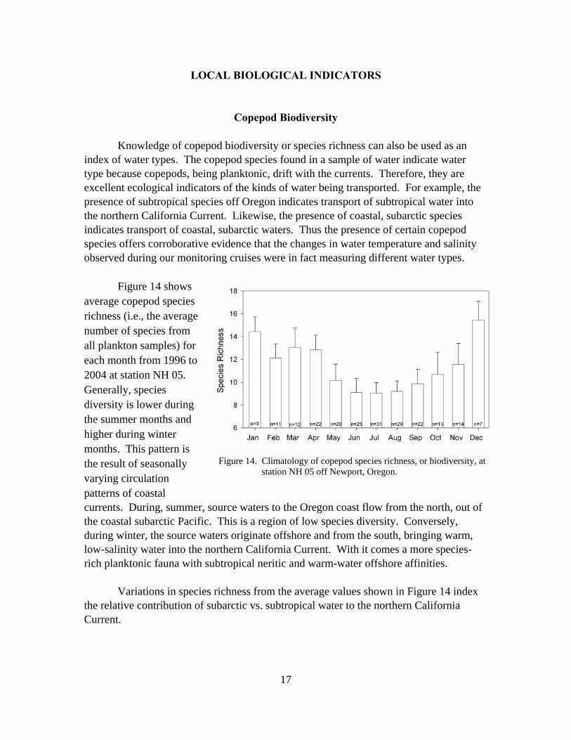
Knowledge of copepod biodiversity or species richness can also be used as an index of water types. The copepod species found in a sample of water indicate water type because copepods, being planktonic, drift with the currents. Therefore, they are excellent ecological indicators of the kinds of water being transported. For example, the presence of subtropical species off Oregon indicates transport of subtropical water into the northern California Current. Likewise, the presence of coastal, subarctic species indicates transport of coastal, subarctic waters. Thus the presence of certain copepod species offers corroborative evidence that the changes in water temperature and salinity observed during our monitoring cruises were in fact measuring different water types.

Figure 14 shows average copepod species richness (i.e., the averagenumber of species from all plankton samples) for each month from 1996 to 2004 at station NH 05. Generally, species diversity is lower during the summer months and higher during winter months. This pattern is the result of seasonally varying circulation patterns of coastal

currents. During, summer, source waters to the Oregon coast flow from the north, out of the coastal subarctic Pacific. This is a region of low species diversity. Conversely, during winter, the source waters originate offshore and from the south, bringing warm, low-salinity water into the northern California Current. With it comes a more species-rich planktonic fauna with subtropical neritic and warm-water offshore affinities.

Variations in species richness from the average values shown in Figure 14 index the relative contribution of subarctic vs. subtropical water to the northern California Current.

Figure 14. Climatology of copepod species richness, or biodiversity, at station NH 05 off Newport, Oregon.

17

Figure 15. Time series of the PDO (red and blue bars, upper panel) and the MEI (dots and line) versus copepod species richness (lower panel) from 1996 to present. Vertical lines indicate the time lag between long-term persistent shifts in the PDO/MEI, and copepod species richness.

Figure 15 shows monthly anomalies of copepod species richness during 1996-2006. This time series is derived by taking the average number of species for each month, then subtracting the observed monthly average for that month. Also shown in Figure 15 are time-series of the Pacific Decadal Oscillation and Multivariate ENSO Index and copepod species richness. Comparisons among these time series show clear relationships between interannual variability in basin-scale physical climate indicators (PDO and MEI) and copepod species richness anomalies at Newport Oregon.

Note that twopronounced changes in copepod species richness lagged the PDO and MEI by about 6 months. The first of these was in 1998, when a change to a negative anomaly of species richness in December was preceded by sign changes of the PDO in July and the MEI in August. The second pronounced change was seen in 2002, with the shift to a positive anomaly of copepod

species richness in November, which followed changes in the PDO and MEI in August and April, respectively.

We saw earlier (Figure 5) that local sea surface temperatures off Newport showed strong correspondence with the PDO. The interpretation of simultaneous change in sea surface temperature and copepod species richness is that when the PDO is in a cool phase, cold water from the subarctic Pacific dominates the northern California Current. Moreover, there is a time-lag of about 6 months between a changes in the PDO sign and changes in water temperature and copepod species composition. For further detail on the relationships between copepod species richness and oceanographic conditions, see Hooff and Peterson (2006).

18

Northern and Southern Copepod Anomalies

To explore the relationship between water type, copepod species richness, and the PDO, we developed two indices based on the affinities of copepods for different water types. The dominant copepod species occurring off Oregon at NH 05 were classed into two groups: those with cold-water and those with warm-water affinities. The cold-water (boreal or northern) group included the copepods Pseudocalanus mimus, Acartia longiremis, and Calanus marshallae. The warm-water group included the subtropical or southern species Mesocalanus tenuicornis, Paracalanus parvus, Ctenocalanus vanus, Clausocalanus pergens, C. arcuicornis and C. parapergens, Calocalanus styliremis, and Corycaeus anglicus.

The cold-water group usually dominates the Washington/Oregon coastal zooplankton community in summer, whereas the warm-water group usually dominates during winter (Peterson and Miller 1977; Peterson and Keister 2003). This pattern is altered during summers with El Niño events and/or when the PDO is in a positive (warm) phase. At such times the cold-water group has negative abundance anomalies and the warm group positive anomalies. Figure 16 shows the time series of the PDO, along with biomass anomalies of northern and southern copepod species averaged over the months of May through September. Changes in biomass among years can range over more than one order of magnitude. When the PDO is negative, the biomass of northern copepods is high (positive) and biomass of southern copepods is low (negative), and vice versa.

Figure 16. The Pacific Decadal Oscillation (upper), northern copepod biomass anomalies (middle) and southern copepod anomalies (lower), from 1969 through 2005. Biomass values are log base-10 in units of mg carbon m-3 .

19

Figure 17. Regression of northern (upper) and southern copepod anomalies (lower) vs. the PDO. Units of biomass are mg carbon m3 .

Figure 17 shows the same data, but as a scatter gram, with copepod anomalies plotted against the PDO. In both cases, the northern and southern copepod species anomalies are correlated with the PDO. We suggest that the correspondence between PDO and northern and southern copepod anomalies is due to physical coupling between the sign of the PDO, coastal winds, water temperatures, and the types of source waters (and the zooplankton which they contain) that enter into the northern California Current and the coastal waters off Oregon.

When winds are strong from the north (leading to cool water conditions and a PDO with a negative sign), cold-water copepod species dominate the ecosystem. During summers characterized by weak northerly or easterly winds, (such as during 1996, 1997, 2004 and 2005, the PDO is positive, warm water conditions dominate, and offshore animals move onshore into the coastal zone.

Perhaps the most significant aspect of the northern copepod index is that two of the cold water species, Calanus marshallae and Pseudocalanus mimus are lipid-rich species. Therefore, an index of northern copepod biomass may also index the amount of wax-esters and fatty acids being fixed in the food chain. These fatty compounds appear to be essential for many pelagic fishes if they are to grow and survive through the winter successfully. Beamish and Mahnken (2001) provide an example of this for coho salmon.

Conversely, the years dominated by warm-water, or southern copepod species can be significant because these species are smaller and have low lipid reserves. This could result in lower fat content in the bodies of small pelagic fish that feed on these species as opposed to cold-water species. Therefore, salmon feeding on pelagic fish, which have in turn fed on warm-water copepod species, may experience a relatively lower probability surviving the winter.

20

Figure 18. Regression of OPI coho survival on the northern copepod biomass anomalies. The regression excludes the ocean entry years 1970 and 1973. Note that high survival anomalies were seen only in the early 1970s data.

Figure 19. Regression of Snake River Chinook smolt-to-adult return rates (from Scheuerell and Williams 2005) against the northern copepod biomass index. The regression excludes the datum from the year 1998. Predicted SARs are shown by the red circles.

The “northern copepod index” appears to be a good predictor of the survival of hatchery coho salmon. Figure 18 shows the correlation between OPIH coho and anomalies of the biomass of northern copepod biomass. The correlation is based on the year of ocean entry. That is, OPIH values for year + 1 are regressed on copepod biomass in year 1.

Using the relationship shown in Figure 18, and the value of the northern copepod anomaly for summer 2005, we can predict that the percent survival of coho salmon that return in fall 2006 will be very low, on the order of less than 1% of the 2005 juvenile migrant population. This value is comparable to the lowest values ever recorded since the OPIH times series began in 1969. We attribute such low survival to the late spring transition in 2005, anomalously warm ocean conditions, and low plankton biomass that persisted from May through mid-July 2005, a critical period for juvenile coho salmon.

A similar analysis was performed for Snake River spring Chinook (Figure 19) using the smolt-to-adult return rates published by Scheuerell and Williams (2005). The

regression was not as strong as that for coho, being significant only at the P = 0.02 level, and accounted for only 28% of the variability. Snake River spring Chinook that went to sea in 2004 could return at a rate of 2%, similar to returns in 2001 and 2002. However, given the extremely low value of the northern copepod index in 2005, we may expect one of the lowest returns of Snake River spring Chinook in 2007.

21

Figure 20. Hatchery coho survival as a function of the date of spring transition at NH 05 (as indicated by the day of first appearance of a cold-water copepod community).

The Biological Spring Transition

We suggested earlier that the spring transition could be defined in several ways, one of which was the date that cold water first appeared in mid-shelf waters. In Figure 11, we saw coho survival correlated with the date when cold water first appeared at our baseline station, NH 05.

Figure 20 shows a similar relationship, but using the date when a northern (cold-water) copepod community first appeared at station NH 05. This date can also be used to index the spring transition. We believe this date may be a more useful indicator of the transition in ocean conditions because it also indicates the first appearance of the kind of food chain that coho and Chinook salmon seem to prefer; that is, one dominated by by large, lipid-rich copepods, euphausiids, and juvenile forage fish.

Thus we suggest that potential feeding conditions for juvenile salmon are more accurately indexed using both the northern copepod biomass and the biological spring transition date (as compared to an upwelling index, which is presumed to serve as an index of feeding conditions). We say this in light of the following two instances wherein the upwelling index alone fails to correctly indicate feeding conditions.

First, during El Niño years, or years with extended periods of weak El Niño-like conditions, upwelling can still be strong (as in 1998), but can produce a warm, low-salinity, and low-nutrient water type (rather than the expected cold, salty, and nutrient-rich water). Upwelling of this water type results in poor plankton production. A second example of upwelling as a misleading indicator occurred during 2005, when mean total upwelling levels from May to September were “average." However, the zooplankton community did not transition to a cold water community until August. Therefore, in spite of this positive indicator, conditions for salmon feeding, growth, and survival were unfavorable throughout all of the spring and most of the summer.

22

160

140 June

120

100

80

60

40

20

0

Num

ber /

km

2

60

50

40

30

20

10

0

September

1998 1999 2000 2001 2002 2003 2004 2005 2006 1998 1999 2000 2001 2002 2003 2004 2005 2006

Catches of Spring Chinook and Coho Salmon during June and September Trawl Surveys

The number of juvenile salmon caught during trawl surveys can serve as an index of the survival for both spring Chinook and coho salmon. These catches of juvenile fish are shown in Figure 21.

Figure 21. Average catches of juvenile coho (solid bars) and Chinook salmon (hatched bars) during trawl surveys off the coast of Washington and Oregon: June (left) and September (right) 1998-2005.

Figure 22 shows correlations between catches of yearling Chinook salmon in June and adult Chinook returns two years later, and between catches of yearling coho in September and adult coho returns the following year. Catches of both coho and Chinook in 2005 were the lowest of our study, which began in 1998. This suggests that we should anticipate low returns of coho in 2006 (~1.5%) and low returns of spring Chinook in 2007 (below-average counts at Bonneville).

Figure 22. Catches of juvenile spring Chinook in June (left) are correlated with adult returns of Chinook 2 years later. Catches in June 2005 were the lowest of our time series, at 4.3 fish per km2. Catches of juvenile coho in September (right) are correlated with adult returns of coho 1 year later. Catches in September 2005 were also the lowest of our time series, at 1.0 fish per km2.

23

INDICATORS UNDER DEVELOPMENT

A Second Mode of North Pacific Sea Surface Temperature Variation

Changes in sign of the PDO tend to follow an east/west dipole; that is, when the North Pacific is cold in the west, it is warm in the east, and vice versa. Bond et al. (2003) showed that variability of sea surface temperature has a second mode, which reflects north/south variations. This pattern first appeared in 1989 and continues to the present.

We have not yet investigated this pattern fully because the negative phase of the first mode (the PDO) indicates favorable conditions in the northern California Current, as does the negative phase of the second mode (called the “Victoria” mode). However, oscillation in the second mode would index good vs. poor ecological conditions between the Gulf of Alaska and northern California. Therefore, it is possible that this second mode may serve as a better index of conditions for spring Chinook salmon, as conventional wisdom is that spring Chinook resides in the Gulf of Alaska during most of its years at sea.

Phytoplankton Biomass

Based on samples collected along the Newport Hydrographic Line, we developed time series of both total chlorophyll and the fraction of chlorophyll smaller than 10 µm. These data serve as estimates of phytoplankton biomass, and both data types will be used to describe interannual variation in timing of the spring bloom (which can occur between February and April), as well as blooms in summer during July-August upwelling. These measures should give an index of the potential conditions (good vs. poor) for spawning of copepods and euphausiids.

Euphausiid Egg Concentration Adult Biomass, and Production Rates

Euphausiids are a key prey item for juvenile coho and Chinook salmon. Sampling along the Newport Hydrographic Line has also yielded a time series of euphausiid egg abundance. These data may serve as an adult euphausiid biomass index, which should prove useful in comparisons of interannual variation in abundance, survival, and growth for these salmon species.

25

Since 2000, we have also been sampling at night along the Newport Line in order to capture adult euphausiids. The long-term goal of this sampling is to produce an index of euphausiid biomass in the northern California Current. We are also measuring rates of molting and egg production in living animals in anticipation that these data can be used to calculate euphausiid production.

Interannual Variations in Habitat Area

From the salmon trawl surveys conducted in June and September, we are developing “Habitat Suitability Indices” which we hope will prove useful in providing more precise predictors of the potential success or failure for a given year-class of juvenile salmonids. For example, we have determined that chlorophyll and copepod biomasses are the best predictors of habitat size for juvenile Chinook. Interannual variation in potential habitat area may also serve as a correlate for salmon survival during the first summer at sea.

Copepod Community Structure

We are developing habitat indices based on use of presence/absence of specific copepod community types observed during the juvenile salmon surveys in June and September. That is, we are attempting to determine if copepod species or community structure are a better descriptor of habitat suitability than bulk measures of biomass such as chlorophyll and copepod biomass.

Forage Fish and Pacific Hake Abundance

We plan to develop an index that describes food-web interactions between juvenile salmon and their fish predators, chiefly Pacific whiting, also known as Pacific hake. The index will be based on interactions between forage fish (e.g., anchovies, smelt and herrings), juvenile salmon, and hake.

This interaction is somewhat complex and probably non-linear: the hypothesis is that during most warm years, hakes move into continental shelf waters, where salmon may be more susceptible to predation. During cold years, hakes feed in deeper waters offshore, near the shelf break; thus they may not be actively feeding in water inhabited by juvenile salmon.

26

During cold conditions, where zooplankton production is high, small forage-fish biomass increases. The advantage to salmon of high forage-fish abundance is that predators are more likely to “see” forage fish than salmon because there are far more of them present in the water column. Since forage-fish populations do well during cold conditions but tend to crash during warm conditions, there will likely be time lags of one or more years between boom and bust periods. Thus, the interaction among zooplankton production, forage-fish abundance, juvenile salmon survival, and hake predation is likely to be non-linear.

Forage Fish density anomalies Pacific Hake density anomalies

-4000

-3000

-2000

-1000

0

1000

2000

3000

4000

Ano

mal

y (N

x 1

06/m

3)

-100

-50

0

50

100

150

Ano

mal

y (N

x 1

06/m

3)

1998 1999 2000 2001 2002 2003 2004 2005 1998 1999 2000 2001 2002 2003 2004 2005

Figure 23. Anomalies in forage fish and Pacific whiting (hake) abundance, 1996-2006.

We have not yet initiated any sophisticated analysis or modeling of these interactions. Figure 23 shows the time series data, and from these it is clear that there are pronounced interannual differences in abundance, and that they are in part related to the ocean-condition cycles discussed in this report.

For Pacific hake, (Figure 23) note that low abundances were observed during the 4-year cool period of 1999-2002, and high abundances occurred during two of the warm years (1998 and 2003). These correspond respectively to “good” and “poor” periods for coho survival. We expected high abundance levels for hake in 2004 and 2005, but this expectation was not met, due possibly to the timing of its northward migration. That is, hake may have moved further north (off Canada) during the warm years of 2004 and 2005, and thus may have been a key predator on salmon only early in the season (May rather than June/July).

Forage fish on the other hand, clearly show a 1-year lag between change in ocean phases and population response: anomalously low abundances were observed during the first year of a “cool phase” (1999), and anomalously high abundances were observed during the first year of “warm phase” (2003). Given the failure of hake to maintain high abundances in 2003 and 2005, and the 1-year lag in response of forage fish to changes in ocean conditions, there were no simple linear relationships between either salmon catches or survival and forage fish or hake.

27

Salmon Predation Index

A salmon predation index will integrate four variables found to influence predation rates of Columbia River salmon in the ocean (Emmett 2006). These variables are based on the following spring (May/June) measurements:

(1) Abundance of Pacific whiting (hake) off the Columbia River (2) Abundance of forage fish off the Columbia River (3) Turbidity of the Columbia River (4) Columbia River flows

Predator and forage fish abundances are estimated annually from the Predator/Forage Fish Survey, and turbidity will be estimated using satellite imagery, Secchi disc readings, and transmissometer measurements, each of which has been collected since 1998. Initial analyses indicates that during years when hake abundance is low and forage-fish abundance, turbidity, and Columbia River flows are high, salmon marine survival is high. However, if even one variable has an opposite value, salmon marine survival declines.

Potential Indices for Future Development

Remaining indices are in very early stages of development or have not yet begun to be developed. These include:

(1) An index of Columbia River flow

(2) Predictors of coho and spring Chinook jack returns

(3) Indices based on salmon feeding and growth

(4) Indices based on salmon health (diseases and parasites)

(5) Indices that estimate zooplankton production rates, such as

• Euphausiid growth rates from direct measurement of molting rates • Euphausiid growth rates from cohort developmental rates • Copepod growth rates from direct measurement of Calanus egg

production rates • Copepod growth rates from empirical growth equations

28

FORECAST of COHO and CHINOOK ADULT RETURNS in 2006 and 2007

Almost all ecosystem indices measured in 2005 point to low adult returns of coho salmon in 2006 and spring Chinook salmon in 2007. From late 2002 through 2005, the PDO has been positive, and coastal ocean temperatures have remained 1-2°C above normal. Both of these indicators signal unfavorable ocean conditions for these two salmon species.

In addition, the spring transition date was very late (i.e., strong and sustained upwelling did not start until mid-July) and copepod species diversity was high. Also in 2005, a large negative anomaly in the northern (cold water) copepod biomass occurred. This anomaly was nearly as large as the largest yet recorded, which occurred during the 1998 El Niño. Moreover, we collected the fewest numbers of juvenile salmon during June and September 2005 than during any of our previous trawl surveys, even those conducted during the 1998 El Niño. Thus, nearly all indicators suggest smolt-to-adult returns rates of no more than 1% for both coho salmon in 2006 and spring Chinook salmon in 2007. Below we examine and interpret the indicators presented in this report as an example of their practical application.

Physical Ocean Conditions

La Niña. In late 2005, NOAA scientists issued a prediction that a La Niña event was developing at the equator. This is a positive indicator because such events usually lead to an earlier start to the northern California Current upwelling season, increased ocean productivity, and greater reproductive success for many species.

However, we know that time lags exist between initiation of an El Niño or La Niña event and a response in Pacific Northwest waters. For example, in 1999, a period of strong upwelling and colder upper-ocean temperatures followed two exceptionally warm years in the northern CC. Yet, this cooler period did not lead to immediate increases in zooplankton, forage fish, or salmon abundance. Rather, there was a 1-year lag, so that it was not until 2000 that a rebound was observed in zooplankton, forage fish, and salmon numbers. Therefore, although early indicators point to favorable physical ocean conditions in 2006, expectations for a quick rebound of salmon stocks should be viewed with caution because ecological conditions have yet to change in salmon-friendly ways. Also, if the recent change in sign of the MEI to positive (in June 2006) continues, we can expect warm ocean conditions to return.

29

Spring Transition. The time when the northern California Current changes from a winter state to a summer state is known as the “spring transition.” If the transition arrives early (March-April), we can expect a lengthy and productive upwelling season. If the transition is late (June-July) we can expect less production and disappointing salmon returns. In 2006, the transition occurred on or before 3 May. This was a relatively early date; a positive indicator for salmon that entered the ocean this spring. However, winter-like storms persisted for 3 weeks (late May to mid-June) and may have reset the ecosystem to a winter state. Sustained coastal upwelling did become established by the end of June 2006.

Biological Indicators

Copepod Biodiversity. Copepod biodiversity, or species richness, has been anomalously high since November 2002, and has remained high through 2006. This is a negative indicator.

Northern Copepod Biomass Index. The northern copepod index tracks anomalies in the summer-averaged biomass of three cold-water copepod species. Because the index is based on average biomass from May to September, it will not be available until late 2006. We can report that the northern “cold water" copepod community did not dominate the zooplankton until late June 2006. This is a negative indicator for early ocean survival of coho salmon smolts and points to below-average returns of coho in 2007 and Chinook in 2008.

June Trawl Survey. Catches of spring Chinook salmon in June are correlated with adult spring Chinook returns two years later. Because these catches were very low during our June 2005 survey, we anticipate low adult returns in spring 2007. Catches from June 2006 were moderate, a positive sign for 2008.

September Trawl Survey. Catches of coho salmon in our September trawl survey are correlated with adult coho returns the following year. Catches in September 2005 were the lowest of our 9-year time series, suggesting poor returns in fall 2006. Catches in our September 2006 survey were also low, a negative indicator.

Forage Fish Abundance. As of July 2006, forage fish abundance continued to remain at low levels, similar to those observed in 1999. This is a negative indicator.

30

REFERENCES

Bakun, A. 1973. Coastal upwelling indices, west coast of North America, 1946–71. U.S. Department of Commerce, NOAA Technical Report NMFS-SSRF-671.

Bakun, A. 1996. Patterns in the ocean: ocean processes and marine population dynamics. California Sea Grant Program, University of California, La Jolla.

Beamish, R. J., and C. Mahnken. 2001. A critical size and period hypothesis to explain natural regulation of salmon abundance and the linkage to climate and climate change. Progress in Oceanography 49:423–437.

Bond, N. A., J. E. Overland, M. Spillane, and P. Stabeno. 2003. Recent shifts in the state of the North Pacific. Geophysical Research Letters: 30(23)2183.

Emmett, R. L. 2006. The relationships between fluctuations in oceanographic conditions, forage fishes, predatory fishes, predator food habits, and juvenile salmonid marine survival off the Columbia River. Ph.D. Thesis, Oregon State University, Corvallis.

Fessenden, L. M. 1996. Calanoid copepod diet in an upwelling system: phagotrophic protists vs. phytoplankton. Ph.D. Thesis, Oregon State University, Corvallis.

Gunsolus, R. T. 1978. The status of Oregon coho and recommendations for managing the production, harvest, and escapement of wild and hatchery-reared stocks. Oregon Department of Fish and Wildlife, Clackamas, OR.

Hooff, R. C., and W. T. Peterson. 2006. Copepod biodiversity as an indicator of changes in ocean and climate conditions of the northern California current ecosystem. Limnology and Oceaonography 51(6):2607-2620. (Available via the internet at www.ASLO.org).

Logerwell, E. A., N. J. Mantua, P. W. Lawson, R. C. Francis, and V. N. Agostini. 2003. Tracking environmental processes in the coastal zone for understanding and predicting Oregon coho (Oncorhynchus kisutch) marine survival. Fisheries Oceanography 12(6):554-568.

31

Mantua, N. J., S. R. Hare, Y. Zhang, J. M. Wallace, and R. C. Francis. 1997. A Pacific decadal climate oscillation with impacts on salmon. Bulletin of the American Meteorological Society 78:1069-1079.

Miller, C. B., H. P. Batchelder, R. D. Brodeur, and W. G. Pearcy. 1985. Response of the zooplankton and ichthyoplankton off Oregon to the El Niño event of 1983. Pages 185-187 in Worster, W. W., and D. L. Fluharty, editors. El Niño North. Washington Sea Grant Program, University of Washington, Seattle.

Nickelson, T. E. 1986. Influences of upwelling, ocean temperature, and smolt abundance on marine survival of coho salmon (Oncorhynchus kisutch) in the Oregon Production Area. Canadian Journal of Fisheries and Aquatic Sciences 43:527-535.

Pearcy, W. G. 1992. Ocean Ecology of North Pacific Salmonids. Washington Sea Grant Program, University of Washington Press, Seattle.

Peterson, W. T., and J. E. Keister. 2003. Interannual variability in copepod community composition at a coastal station in the northern California Current: a multivariate approach. Deep Sea Research Part II: Topical Studies in Oceanography 50(14-16):2499-2517.

Peterson, W. T., and C. B. Miller. 1975. Year-to-year variations in the planktology of the Oregon upwelling zone. Fishery Bulletin, U.S. 73:642-653.

Peterson, W. T., and C. B. Miller. 1977. Seasonal cycle of zooplankton abundance and species composition along the central Oregon coast. Fishery Bulletin, U.S. 75:717-724.

Scheuerell, M. D., and J. G. Williams. 2005. Forecasting climate-induced changes in the survival of Snake River spring/summer Chinook salmon (Oncorhynchus tshawytscha). Fisheries Oceanography 14(6):448-457.

Ware, D. M., and G. A. McFarlane. 1989. Fisheries production domains in the Northeast Pacific Ocean. Pages 359-379 in Beamish, R. J., and G. A. McFarlane, editors. Effects of ocean variability on recruitment and an evaluation of parameters used in stock assessment models. Canadian Special Publication of Fisheries and Aquatic Sciences 108, Ottawa, Ontario.

32

APPENDIX A

Introduction to the Local Oceanography

Physical Oceanographic Considerations

The marine and anadromous faunae over which NOAA Fisheries exercises stewardship occupy diverse habitats in the coastal ocean off Washington, Oregon, and California. This biogeographic region has been collectively termed the Coastal Upwelling Domain (Ware and McFarlane 1989). Dominant fisheries species within this domain include market squid, northern anchovy, Pacific sardine, Pacific hake, Pacific mackerel, jack mackerel, Pacific herring, rockfish, flatfish, sablefish, and coho and Chinook salmon.

Within this domain, several smaller-scale physical zones are recognized, including

(a) A near-shore zone where juvenile fall Chinook salmon, sand lance, and smelts reside

(b) The upper 10-20 m of the water column across the continental shelf and slope, where many pelagic fishes reside, including juvenile coho and Chinook

(c) The benthic and demersal habitats on the continental shelf (English sole), at the shelf break (whiting, rockfish), and beyond the shelf break to depths of 1500 m (sablefish, Dover sole, and thornyheads).

Each of these physical zones has unique circulation patterns that affect spawning and larval transport, and each is subject to different physical conditions. These differing conditions lead to species-specific variations in growth, survival, and recruitment. Moreover, since many species have pelagic larvae/juvenile stages, recruitment is affected by boad-scale variations both in ocean productivity, which affects the feeding environment of larval and juvenile fish, and in ocean circulation, which affects the transport of eggs and larvae.

The Coastal Upwelling Domain is part of the California Current system, a broad, slow, meandering current that flows south from the northern tip of Vancouver Island (50EN) to Punta Eugenia near the middle of Baja, California (27EN). The California Current extends laterally from the shore to several hundred miles from land. In deep oceanic waters off the continental shelf, flows are usually southward all year round. However, over the continental shelf, flows are southward only in spring, summer, and

33

fall: during winter, flow over the shelf reverses, and water moves northward as the Davidson Current.

These biannual transitions between northward and southward flow over the shelf occur in during March-April and October-November and are respectively termed the "spring transition" and "fall transition." Another important feature of circulation within the Coastal Upwelling Domain is the deep, poleward-flowing undercurrent found year-round at depths of 100-300 m over the outer shelf and slope. This current seems to be continuous from Southern California (33ºN) to the British Columbia coast (50ºN).

Coastal upwelling is the dominant physical element affecting production in the Coastal Upwelling Domain. In the continental shelf waters off Washington and Oregon, upwelling occurs primarily from April to September, whereas upwelling can occur year-round off the coasts of northern and central California. Upwelling in offshore waters also occurs through Ekman pumping and surface divergence in the centers of cyclonic eddies, but these processes will not be discussed further here.

Coastal upwelling works as follows: winds that blow from the north (towards the equator) result in the offshort transport of waters within the upper 15-m of the water column. This offshore transport of surface waters is balanced by onshore movement of cold, nutrient-rich waters from a depth of about 100-125 m at the shelf-break region. When winds are strong, this cold (8EC), nutrient-rich water surfaces within 5 miles of the coast. The result is high production of phytoplankton from April through September fueled by a nearly continuous supply of nutrients and concomitant high biomass of copepods, euphausiids, and other zooplankton during summer.

Coastal upwelling is not a continuous process. Rather, it is episodic, with favorable (equatorward) winds blowing for 1-2 week periods, interspersed by periods of either calm or reversals in wind direction. These pulses in the winds produce what are called “upwelling events.” Interannual variations in the length and number of upwelling events result in striking variations in the level of primary and secondary production. Thus, the overall level of production during any given year is highly variable, and is dependent on local winds.

34

We do not yet know if there is an optimal frequency in upwelling event cycles, but one can easily imagine scenarios in which prolonged periods of continuous upwelling would favor production in offshore waters because nutrient-rich waters would be transported far to sea. The other extreme is one in which winds are weak and produce upwelling only in the very nearshore zone, within a mile or two of the coast. In this case, animals living in waters off the shelf would be disadvantaged. Any process that leads to reduction in the frequency and duration of northerly winds will result in decreased productivity and vice versa. The most extreme of these processes is El Niño, which disrupts coastal ecosystems every 5-10 years.

Despite the existence of high plankton biomass and productivity, coastal upwelling environments present unique problems to fish and invertebrate populations who must complete their life cycles there. This is because the upwelling process transports surface waters and the associated pelagic larvae and juvenile life stages away from the coast and towards the south, away from productive habitats. Typical transport rates of surface waters are 1 km per day in an offshore direction and 20-30 km per day southward.

Zooplankton and larval and juvenile fishes, which live in the food-rich surface layers (i.e., the upper 15 m of the water column ), can be transported rapidly offshore, out of the upwelling zone, and into relatively oligotrophic waters. Bakun (1996) argues that for any animal to be successful in such environments, the adults must locate habitats that are characterized by enrichment, with some mechanism for concentrating food (for larvae), and that offer a way for larvae to be retained within the system.

Perhaps because of its problems related to transport (and loss), many species do not spawn during the upwelling season. Species such as Dover sole, sablefish, Dungeness crab, and pink shrimp each spawn during the winter months, before the onset of upwelling. Other species perform an extended migration to spawn in regions where there is no upwelling.

Hake, for example, undertakes an extended spawning migration, during which adults swim south to spawn in the South California Bight in autumn and winter, outside of the upwelling region and season. This migration extends from Vancouver Island (ca. 49EN) to southern California (35EN), a distance of several thousand kilometers. The return migration of adults and the northward drift of larvae and juveniles take place at depth, where fish take advantage of the poleward undercurrent.

Still other species, such as English sole, spawn in restricted parts of an upwelling system where advective losses are minimized, such as in bays or estuaries. Salmonids

35

and eulachon smelt spawn in rivers, completely outside the upwelling system. Finally, species such as rockfish simply bypass the egg and larval stages and give birth to live precocious "juvenile" individuals.

Variability in the Physical Environment at Climatic Scales

Variability in productivity of the California Current occurs at climatic time scales, each of which must be taken into account when considering recruitment variability and fish growth. The North Pacific experiences dramatic shifts in climate every 10-20 years. These shifts occurred in 1926, 1947, 1977, and 1998 and were caused by eastward-westward jumps in the location of the Aleutian Low5 in winter, which result in changes in wind strength and direction. Changes in large-scale wind patterns lead to alternating states of either “a warm ocean climate regime” or “cold water regime,” with a warm ocean being less productive than a cold ocean.

Changes in biological productivity are best documented for the period since the 1950s, and this understanding is largely due to measurements made by the California Cooperative Oceanic Fisheries Investigations (CalCOFI) program. Zooplankton biomass, for example, was high from the 1950s through 1977, but during the warm regime of 1977-1998, zooplankton biomass in the southern sector of the California Current declined by nearly one order of magnitude. In the northern California Current, the change in zooplankton biomass between regimes was not as dramatic, ranging just over one-half an order of magnitude in coastal waters off Newport Orgeon. Zooplankton biomass was higher than average during the cool regime prior to 1977 and lower than average durring the warm regime from 1977 to 1998. During 2000-2004, zooplankton biomass rebounded to levels comparable to those seen prior to 1977.

Since the early 1980s, the California Current has been experiencing an increased frequency of El Niño events, with large El Niño events occurring every 5-6 years: 1976-77, 1982-83, 1986-87, 1991-92, 1997-98 and again in 2002-2004. A higher frequency of El Niño events appears to be a characteristic of the extended periods of warm ocean conditions. From 1992 to 1998, the Oregon and Washington coasts experienced almost continuous El Niño-like conditions during summer (i.e., reduced upwelling and warmer ocean conditions). Since 1998, ocean conditions have improved markedly, and it appears that another regime shift may have been initiated in late 1998. Thus the California Current now appears to have returned to a cool, productive phase. The shift to productive conditions was interrupted for three years (late 2002-late 2005), but the ocean has once again cooled (in early 2006). Whether or not short-term (3-4 year) variability will become the norm remains to be seen.

36

__________________________________

Alaska

BritishColumbia

U.S.

ALASKACURREN

Cold Phase

CALIFO

NI

CU

RR

ENT

Alaska

BritishColumbia

U.S.A

ALASKACURRE

T

Warm Phase

CA

IFN

IA

CU

RR

ET

Alaska

BritishColumbia

U.S.

T

ALASKACURREN

Cold Phase

CALIFO

NI

CU

RR

ENT

C

Alaska

BritishColumbia

U.S.A

N

ALASKACURRE

T

Warm Phase

CA

IFN

IA

CU

RR

ET

656565 656565

606060 606060

555555 555555

505050 505050

454545 454545

404040 404040

353535 353535

303030 303030

171717000 111666000 111555000 111404040 130130130 121212000 111101010252525

170170170 160160160 150150150 140140140 130130130 120120120 110110110252525

A.WEST WIND DRIFT

R

A

A.WEST WIND DRIFT

T

RA

Alaska

British olumbia

U.S.A.WEST WIND DRIFT

ALASKACURRENT

Cold Phase

CALIFO

RN

IAC

UR

REN

T

. WEST WIND DRIFT

L O

RN

.WEST WIND DRIFT

N

LO

RN

Alaska

British Columbia

U.S.A.WEST WIND DRIFT

ALASKACURRENT

Warm Phase

CALIFO

RN

IA

CU

RR

ENT

It is unclear why ENSO activity has a variable impact on the Pacific Northwest, but one problem is that we do not know precisely how ENSO signals are transmitted from the equator to the PNW. Signals can arrive through the ocean via Kelvin waves, †

which propagate up the coast of North America. ENSO signals can also be transmitted through atmospheric teleconnections. El Niño conditions can strengthen the Aleutian Low pressure system over the Gulf of Alaska; thus, adjustments in the strength and location of low-pressure atmospheric cells at the equator can affect our local weather. This results in more frequent large storms in winter and disruption of upwelling winds in spring and summer.‡

Appendix Figure Al. A working hypothesis on how changes in the Pacific Decadal Oscillation affect productivity in the northern California Current.

We hypothesize that during “cold PDO” (such 1999-2002), a larger amount of water enters the California Current from the Gulf of Alaska, whereas during “warm PDO” such as 2003-2005, smaller amounts of water enter from the Gulf of Alaska and more enters from the West Wind Drift ¥ offshore or from the south. The changes in the type of source water yield the results shown in Appendix Table A1.

† Kelvin waves ‡ For additional details, see www.cdc.noaa.gov/spotlight/07012001¥ Also known as the Antarctic Circumpolar Current; for further information see the US Office of Naval

Research web page at: www.onr.navy.mil/Focus/ocean/motion/currents1.htm.

37

These simple relationships only hold during years of persistent recurrence of one phase of the PDO or the other. During transitional years, such as 1998-1999, 2002-2003, and possibly 2006, there are time-lags in the ecosystem responses. For example, after the 1998 and 2002 climate shifts, water temperatures lagged the PDO by 1-2 months, changes in copepod biodiversity lagged the PDO index by 4-6 months, and changes in copepod biomass lagged the PDO by two years. Similarly, increases in abundances of forage fish and juvenile salmon lagged the PDO index changes by 1-2 years. If the year 2006 is classified as a “cool phase” year, we might expect a 1-year time lag in response by the salmon to a renewal of “good ocean conditions.”

Appendix Table A1. Summary of the manner in which the sign of the PDO influences broad-scale and local physical ocean condition indicators as well as biological indicators.

Cool PDO Warm PDO

Broad-scale ocean Pacific Decadal Oscillation values negative positive Multivariate ENSO Index values negative positive Local physical indicators

Upwelling not necessarily related to either phase Physical spring transitiona not necessarily related to either phase Sea surface temperatures cold warm Water type in continental shelf waters cold and salty warm and fresh

Local and regional biological indicators Copepod species richness low high

Northern copepod biomass positive anomaly negative anomaly Southern copepod biomass negative anomaly positive anomaly

Euphausiid egg abundance in shelf water usually high usually low Biological spring transition early late

Trawl surveys Coho abundance high low

Spring Chinook abundance high low Coho survival b high low Developing indicators Snake River Chinook SAR c high low

Forage fish abundances many few Pacific hake abundances few many

a (Logerwell et al. 2003) b (OPIH) Oregon production index, hatcher:c Smolt-to-adult returns (see Scheurell and Williams 2005)

38

APPENDIX B:

At-Sea Sampling Methods

Hydrography, Zooplankton, and Ichthyoplankton

Much of the oceanographic data shown in this report came from sampling along the Newport Hydrographic Line (arrow in figure below). During the upwelling season in spring, summer, and fall, we sample the coastal waters off Newport at biweekly intervals. Sampling cruises are conducted monthly during stormy winter months. This program began in 1996, but we also have data from these same stations from sampling conducted in 1973 (Peterson and Miller 1975), 1983 (Miller et al. 1985), and summer 1990-1992 (Fessenden 1995). Most data presented here are from the cruises initiated in May 1996.

From May 1996 through September 2001, all cruises were made during daylight hours because our research vessel, the RV Sacajawea was only 37 ft in length rendering it unsafe to work at night. With the acquisition of a new (and larger, 55 ft) research vessel in September 2000, we were able to sample at night. Thus in fall 2000, we began collecting data for an adult euphausiid time series.

This work includes measurements of copepod and euphausiid egg production and molting rates. Thus we are also developing a long time-series of copepod and euphausiid production, which should prove useful in evaluating if in fact there are measurable differences in zooplankton production in association with changes in sign of the Pacific Decadal Oscillation. Appendix Figure B1. Transects and stations sampled during

cruises by the NOAA Fisheries Service.

39

At each station, a CTD profile (conductivity, temperature, and depth) is taken (Seabird SBE 19+ CTD), and transparency of surface waters is measured (Secchi disc). A bucket of seawater is collected from the surface for analysis of chlorophyll-a and nutrients. A vertical plankton net fitted with a flowmeter is towed from near the sea floor to the surface (or from 100 m to the surface in deeper waters). The plankton net is 0.05 m in diameter with a mesh size of 202 Fm. A double-oblique tow‡ is made for ichthyoplankton (1-m-diameter net with 333-Fm mesh) over the upper 20 m. Since 2005, CTD casts have included fluorometry (WetLabs fluorometer) and oxygen (Seabird oxygen sensor).

From 1998 to 2003, we sampled each transect line five times per year as part of the U.S. Global Ocean Ecosystem Dynamics (GLOBEC) program. Since the GLOBEC project ended, we have continued to sample these same transect lines as frequently as possible. Thus far, we have been able to sample each transect in May (2004-2006), along with several visits to the Newport Line, out to 85 miles from shore, in summer 2004. As a result, the Newport biweekly data are nested within larger-scale quarterly surveys, an approach that is useful in helping us interpret locally derived data from the inner portions of the Newport Line.

Nutrients are analyzed using a Technicon Autoanalyzer. Chlorophyll-s is extracted from glass-fiber filters in 90% acetone then analyzed using a Turner Designs Fluorometer. Zooplankton samples are processed in the laboratory by subsampling with a Stempel pipette. Species and developmental stage of copepods are enumerated with the aid of a dissecting microscope. Counts are converted to number of individuals per m3 of water using appropriate conversion factors. Biomass is estimated by multiplying the number of individuals per m3 by the dry weight of the taxa (using values from either literature or our own measurements). Carbon content is calculated assuming carbon is 40% of dry weight.

Juvenile Salmon Sampling Program

Methods--We have been sampling juvenile salmon off the coasts of Washington and Oregon at the stations shown in the figure below, in June and September, since 1998. Pelagic fish are collected within the upper 20 m of the water column with a NET Systems Model 264 rope trawl (30 m wide × 20 m high × 100 m long), at stations ranging from Newport, Oregon north to La Push, Washington (Appendix Figure B2). For each trawl sample, all fish and invertebrates are identified and enumerated. Lengths of 50 randomly

‡ An oblique tow is made by pulling the net at a slow tow speed from the sea floor to the surface. Under this configuration, the angle between the net and sea floor is oblique .

40

selected individuals are measured. For juvenile salmon, up to 200 individuals of each species and size class (i.e., subyearling and yearling Chinook based on size) are measured and individually frozen at -20°C.

Oceanographic data collected at each station include continuous underway sampling of sea surface temperature and salinity, depth profiles of salinity and temperature with a CTD (Seabird SBE-19 plus) and water transparency (Secchi depth and transmissometer). A water sample is collected from a depth of 3 m for analysis of chlorophyll-a (filtered through glass-fiber filters). The filtrate is frozen for later analysis of nutrient concentrations (nitrate, silicate, phosphate). BPA Plume Study

LaPush

Astoria

Tillamook

Newport

LP04

LP06

LP09

LP12

LP17

LP22

LP27

QR0

3

QR0

6

QR1

0

QR1

4

QR1

9

QR2

4

QR2

9

QR3

4

GH0

3

GH0

6W

B05

Cape Meares

La Push

GH1

0

GH1

6

GH2

1

GH2

6

GH3

1

GH3

6

WB0

9

WB1

4

WB1

9

WB2

3

WB3

0

CR04

CR07

CR10

CR15

CR20

CR25

CR30

CR35

CR40

CR45

CR50

CF01

CF03

CF07

CF10

CF15

CF20

CF25

CF30

CM

01C

M03

CM

05

CM

10

CM

15

CM

20

CM

25

CH0

1C

H02

CH0

5

CH1

0

CH1

5

CH2

0

CH2

5

NH03

NH05

NH10

NH15

NH20

NH25

Washington

Oregon

Newport

Cascade Head

Columbia River

Willapa Bay

Grays Harbor

Cape Falcon

Queets River

Target Station Locations

48° N

47° N

46° N

45° N

125° W 124° W 123° W

Zooplankton is collected by vertical plankton tow (0.5-m diameter, 200-µm mesh) and an oblique bongo tow (60-cm diameter, 333-µm mesh bongo) from 20 m to the surface.

We (Robert Emmett) also carry out cruises every 10 days during which pelagic fish are sampled at night along transects off the Columbia River and Willapa Bay. This work provides data to index the abundance of fish predators (such as hake) and forage fish (which can serve as an alternate prey of the fish predators).

From 1998 to 2005, we have collected samples over a wide range of ocean conditions. These data have provided many insights into the role of ocean conditions in controlling survival and growth of coho and Chinook salmon. For example, we sampled during a very strong El Niño (June 1998) and a strong La Niña (cold-water) (1999), under very high Columbia River flows (June 1999) and extremely low flows (June 2001), and during anomalously warm conditions in the coastal ocean due to lack of upwelling (June 2005). Also during this 8-year

Appendix Figure B2. Transects sampled for coho andyearling and subyearlingChinook salmon, 1998-2006.

period, the Pacific Decadal Oscillation moved from warm phase (pre-1999), to cool phase (1999-2002), then to warm phase again (2003-2005). Thus, nature has handed us a grand experiment that allows us to determine in what ways and how quickly salmon and other ecosystem components respond to short-term climate variability.

41

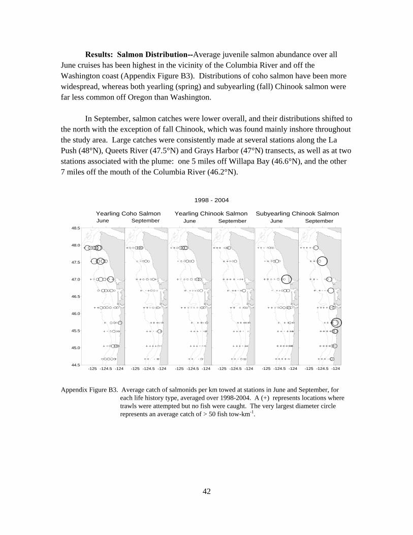
Results: Salmon Distribution--Average juvenile salmon abundance over all June cruises has been highest in the vicinity of the Columbia River and off the Washington coast (Appendix Figure B3). Distributions of coho salmon have been more widespread, whereas both yearling (spring) and subyearling (fall) Chinook salmon were far less common off Oregon than Washington.

In September, salmon catches were lower overall, and their distributions shifted to the north with the exception of fall Chinook, which was found mainly inshore throughout the study area. Large catches were consistently made at several stations along the La Push (48°N), Queets River (47.5°N) and Grays Harbor (47°N) transects, as well as at two stations associated with the plume: one 5 miles off Willapa Bay (46.6°N), and the other 7 miles off the mouth of the Columbia River (46.2°N).

1998 - 2004

Yearling Coho Salmon Yearling Chinook Salmon Subyearling Chinook Salmon June September June September June September

-125 -124.5 -124 -125 -124.5 -124 -125 -124.5 -124 -125 -124.5 -124 44.5

45.0

45.5

46.0

46.5

47.0

47.5

48.0

48.5

-125 -124.5 -124 -125 -124.5 -124

Appendix Figure B3. Average catch of salmonids per km towed at stations in June and September, for each life history type, averaged over 1998-2004. A (+) represents locations where trawls were attempted but no fish were caught. The very largest diameter circle represents an average catch of > 50 fish tow-km-1.

42

Catches in both June and September were also very patchy in that we generally caught half of the fish in less than 5 trawls per cruise and did not catch any fish in 40% of the trawls. Patches most generally occurred for both yearling Chinook and coho off the Washington coast in June (Appendix Figure B3) and very near shore for yearling and subyearling Chinook in September.

Results: Year-to-year variations in salmon abundance--The lowest June catches of Chinook and coho salmon were associated with an El Niño event in 1998 and an anomalously low upwelling period during May and June 2005 (Appendix Figure B4). Highest catches were during the cold phase of the Pacific Decadal Oscillation (1999-2003). Catches of yearling Chinook began to decline in September 2003 in concert with persistent warming, which began that summer and continued through 2005. The number of yearling Chinook caught in September was lower than in June, whereas subyearling Chinook was more abundant in September than June.

Plume Studies Juvenile Salmon

1998 1999 2000 2001 2002 2003 2004 2005 Year

No.

/ km

0

50

100

150

200

250 Coho yearling Chinook yearling Chinook subyearling

Appendix Figure B4. Annual variation in catches of juvenile coho and Chinook salmon during June trawl surveys, 1998-2005.

2

43

APPENDIX C: Web Sites for Addtional Information

http://www.cdc.noaa.gov/ENSO NOAA/El Niño information

http://www.cses.washington.edu/cig/pnwc/cc.shtml University of Washington Climate Impacts Group

http://www.cdc.noaa.gov/people/klaus.wolter/MEI/mei.html Multivariate ENSO index (MEI)

http://www.cses.washington.edu/cig/fpt/orcohofc.shtml, Forecasting of Oregon coho by Logerwell et al.

http://www.pices.int/publications/brochures/PICES%20Advisory%20Report.pdf PICES Marine Ecosystems of the North Pacific

http://www.pac.dfo-mpo.gc.ca/sci/psarc/OSRs/Ocean_SSR_f.htm. Canadian Department of Fisheries and Oceans

http://www.iphc.washington.edu/Staff/hare/html/decadal/post1977/ophi.html Data from the OPIH (Oregon Production Index, Hatchery)

44

http://www.cdc.noaa.gov/ENSO

http://www.cses.washington.edu/cig/pnwc/cc.shtml

http://www.cdc.noaa.gov/people/klaus.wolter/MEI/mei.html

http://www.cses.washington.edu/cig/fpt/orcohofc.shtml

http://www.pices.int/publications/brochures/PICES%20Advisory%20Report.pdf

http://www.pac.dfo-mpo.gc.ca/sci/psarc/OSRs/Ocean_SSR_f.htm

http://www.iphc.washington.edu/Staff/hare/html/decadal/post1977/ophi.html

ocean conditions and salmon survival in the northern ... · 2032 s marine science drive newport,...

Documents