odysseus2015 - koç hastanesihome.ku.edu.tr/~daksen/aksen_odysseus2015.pdf · » there must be...
TRANSCRIPT

Battlefield VRP: Clash of Formulations, Valid Inequalities, Commercial Solvers and Solver Options
Temel Öncan
Galatasaray University Dept. of Industrial Engineering
Ortaköy, İSTANBUL
Deniz Aksen
Koç University College of Admin. Sci. and Econ.
Sarıyer, İSTANBUL
Mir Ehsan Hesam Sadati
Koç University IEOM PhD Program
Sarıyer, İSTANBUL
05 June 2015 Friday

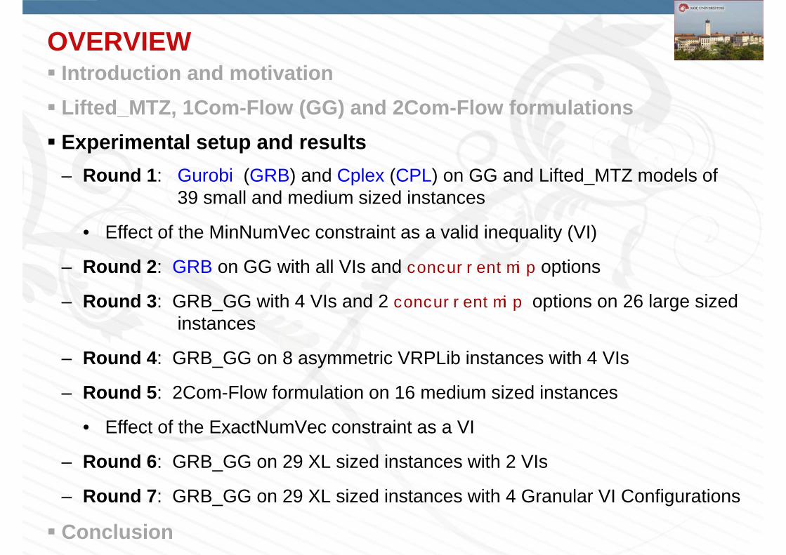
OVERVIEW Introduction and motivation Lifted_MTZ, 1Com-Flow (GG) and 2Com-Flow formulations Experimental setup and results
– Round 1: Gurobi (GRB) and Cplex (CPL) on GG and Lifted_MTZ models of 39 small and medium sized instances
• Effect of the MinNumVec constraint as a valid inequality (VI)
– Round 2: GRB on GG with all VIs and concurrentmip options
– Round 3: GRB_GG with 4 VIs and 2 concurrentmip options on 26 large sized instances
– Round 4: GRB_GG on 8 asymmetric VRPLib instances with 4 VIs
– Round 5: 2Com-Flow formulation on 16 medium sized instances
• Effect of the ExactNumVec constraint as a VI
– Round 6: GRB_GG on 29 XL sized instances with 2 VIs
– Round 7: GRB_GG on 29 XL sized instances with 4 Granular VI Configurations
Conclusion

What motivated us (actually me ;-)
Formulation with polynomial number of subtour elimination orconnectivity constraints:
Only Miller-Tucker-Zemlin (MTZ) inequalities
Everybody knows GG, the Single Commodity Flow Formulation firstproposed by Gavish and Graves (1978)
Almost nobody uses it (except me ;-)
Lack of standards when it come to valid inequalities (VIs).
Everybody devises his or her own VIs. No rigorous testing!
As if Cplex was a combination of iPhone 6 and Mercedes S Klasse.
Haven’t seen any computational OR paper in the past 10years defying this norm!
» There must be quite a few, but they remain in oblivion.
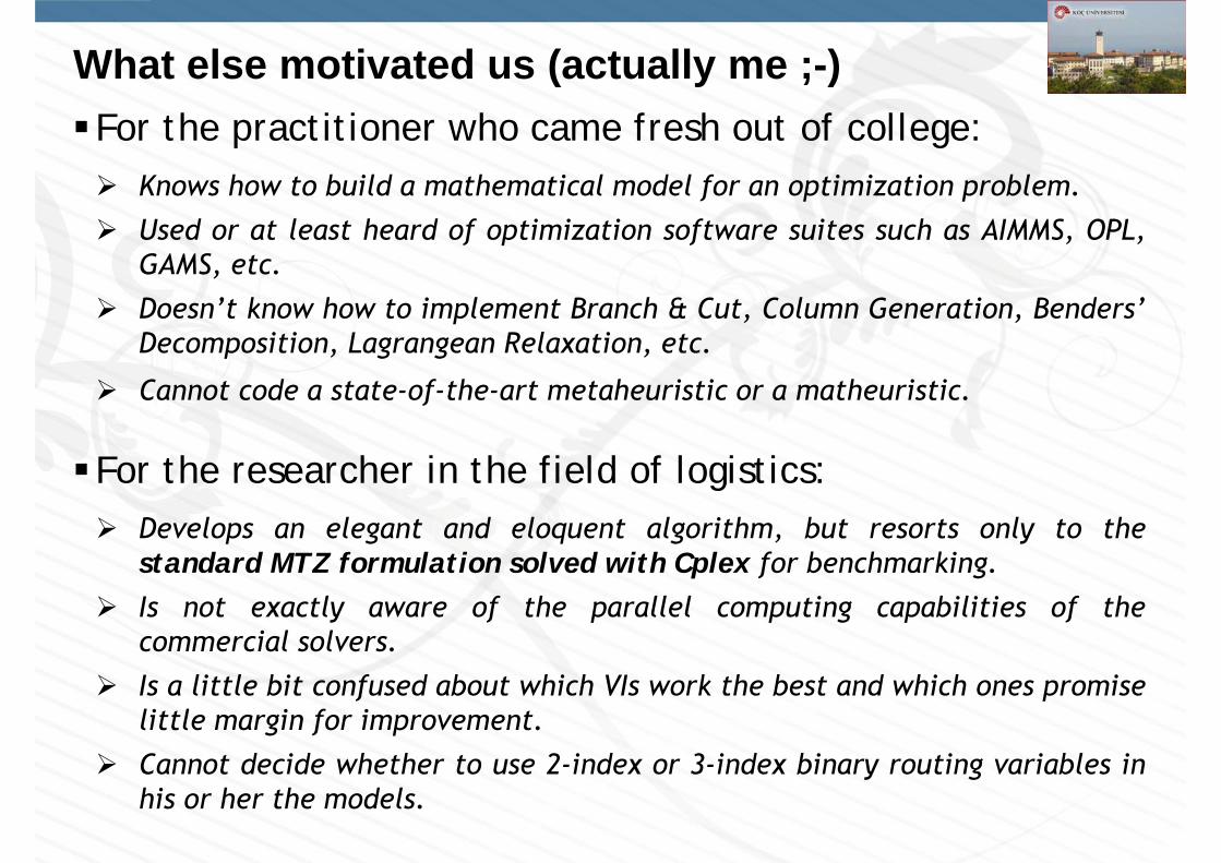
What else motivated us (actually me ;-)For the practitioner who came fresh out of college: Knows how to build a mathematical model for an optimization problem.
Used or at least heard of optimization software suites such as AIMMS, OPL,GAMS, etc.
Doesn’t know how to implement Branch & Cut, Column Generation, Benders’Decomposition, Lagrangean Relaxation, etc.
Cannot code a state-of-the-art metaheuristic or a matheuristic.
For the researcher in the field of logistics: Develops an elegant and eloquent algorithm, but resorts only to the
standard MTZ formulation solved with Cplex for benchmarking.
Is not exactly aware of the parallel computing capabilities of thecommercial solvers.
Is a little bit confused about which VIs work the best and which ones promiselittle margin for improvement.
Cannot decide whether to use 2-index or 3-index binary routing variables inhis or her the models.

OVERVIEW Introduction and motivation Lifted_MTZ, 1Com-Flow (GG) and 2Com-Flow formulations Experimental setup and results
– Round 1: Gurobi (GRB) and Cplex (CPL) on GG and Lifted_MTZ models of 39 small and medium sized instances
• Effect of the MinNumVec constraint as a valid inequality (VI)
– Round 2: GRB on GG with all VIs and concurrentmip options
– Round 3: GRB_GG with 4 VIs and 2 concurrentmip options on 26 large sized instances
– Round 4: GRB_GG on 8 asymmetric VRPLib instances with 4 VIs
– Round 5: 2Com-Flow formulation on 16 medium sized instances
• Effect of the ExactNumVec constraint as a VI
– Round 6: GRB_GG on 29 XL sized instances with 2 VIs
– Round 7: GRB_GG on 29 XL sized instances with 4 Granular VI Configurations
Conclusion
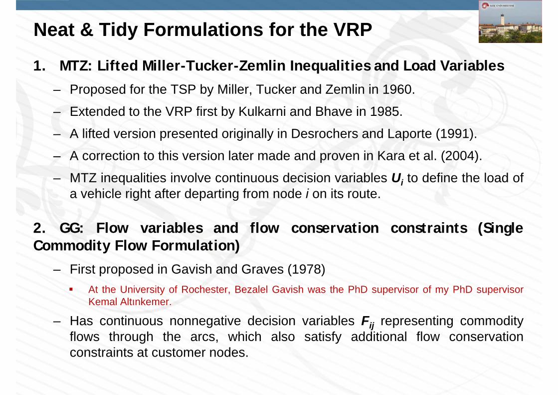
Neat & Tidy Formulations for the VRP
1. MTZ: Lifted Miller-Tucker-Zemlin Inequalities and Load Variables
– Proposed for the TSP by Miller, Tucker and Zemlin in 1960.
– Extended to the VRP first by Kulkarni and Bhave in 1985.
– A lifted version presented originally in Desrochers and Laporte (1991).
– A correction to this version later made and proven in Kara et al. (2004).
– MTZ inequalities involve continuous decision variables Ui to define the load ofa vehicle right after departing from node i on its route.
2. GG: Flow variables and flow conservation constraints (SingleCommodity Flow Formulation)
– First proposed in Gavish and Graves (1978) At the University of Rochester, Bezalel Gavish was the PhD supervisor of my PhD supervisor
Kemal Altınkemer.
– Has continuous nonnegative decision variables Fij representing commodityflows through the arcs, which also satisfy additional flow conservationconstraints at customer nodes.

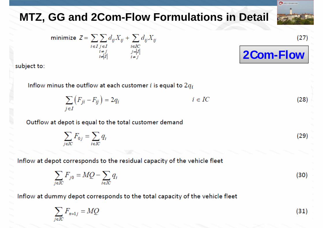
Neat & Tidy Formulations for the VRP 3. 2Com-Flow: Two-Commodity Network Flow Formulation
– Originally introduced by Finke et al. (1984) for the TSP.
– Extended by Langevin et al. (1993) to the TSPTW (TSP with time windows).
– VRP version proposed by Baldacci, Hadjiconstantinou and Mingozzi(the Legendary Troika) in 2004.
– Applies to the symmetric VRP.
We are working on its extension to the asymmetric VRP.
– Uses a dummy depot (n+1) juxtaposed with the original depot (node 0).
– Each customer node including the two depot nodes have one incoming andone outgoing arc the flows of which add up to the uniform vehicle capacity Q.
– For every vehicle route in the solution, the original and dummy depot nodesboth receive a pair of incoming and outgoing arcs.
– The outflow at depot 0 is equal to the total customer demand, and the inflow atthe dummy depot (n+1) corresponds to the total capacity of the vehicle fleet.
– Needs no flow conservation (balance of flow) constraints.
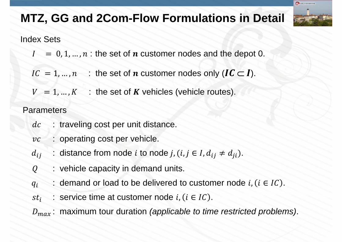
MTZ, GG and 2Com-Flow Formulations in DetailIndex Sets
0, 1, … , : the set of customer nodes and the depot 0.
1, … , : the set of customer nodes only ( ).
1, … , : the set of vehicles (vehicle routes).
Parameters
: traveling cost per unit distance.
: operating cost per vehicle. : distance from node to node , , ∈ , .
: vehicle capacity in demand units.
: demand or load to be delivered to customer node , ∈ .
: service time at customer node , ∈ .
: maximum tour duration (applicable to time restricted problems).

MTZ, GG and 2Com-Flow Formulations in Detail Decision Variables
: total traveling distance (objective function value).
: binary variable indicating if arc , is traversed by a vehicle , ∈ .
: service completion time at node i, i I. 0 is fixed for the depot.
: load of the vehicle right after departing from location i ∈ .
: the amount of goods flowing from node i to node j after collecting the“supply” at node i.
Defining as well as as such as if the VRP is a collection problem ratherthan a delivery problem seems to work better. In other words, variables getbigger from the start of a route towards its end.
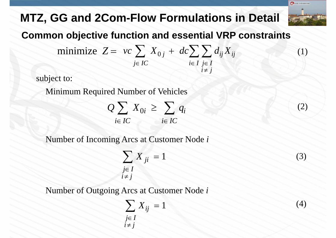
MTZ, GG and 2Com-Flow Formulations in DetailCommon objective function and essential VRP constraints
0
j ij ijj IC i I j I
i j
vc X dc d Xminimize Z (1)
subject to:Minimum Required Number of Vehicles
(2)
Number of Incoming Arcs at Customer Node i
(3)
0
i ii IC i IC
Q X q
1
jij Ii j
X
D 6 Q Total Demand
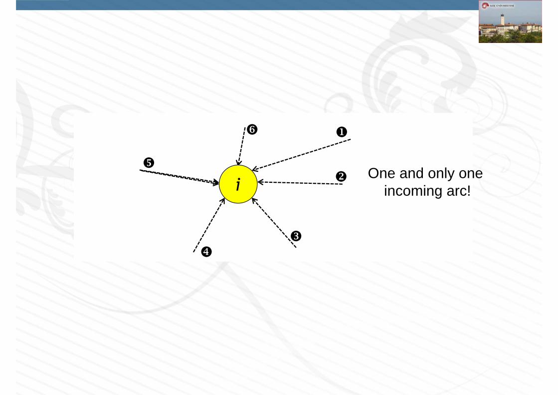
One and only one incoming arc!
i
MTZ, GG and 2Com-Flow Formulations in DetailCommon objective function and essential VRP constraints
0
j ij ijj IC i I j I
i j
vc X dc d Xminimize Z (1)
subject to:Minimum Required Number of Vehicles
(2)
Number of Incoming Arcs at Customer Node i
(3)
Number of Outgoing Arcs at Customer Node i(4)
0
i ii IC i IC
Q X q
1
jij Ii j
X
1
ijj Ii j
X
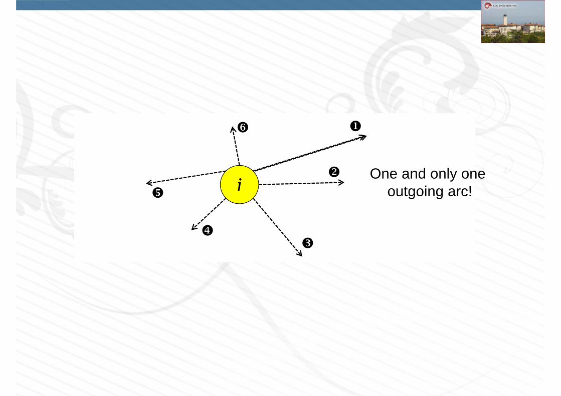
One and only one outgoing arc!
i
MTZ, GG and 2Com-Flow Formulations in Detail
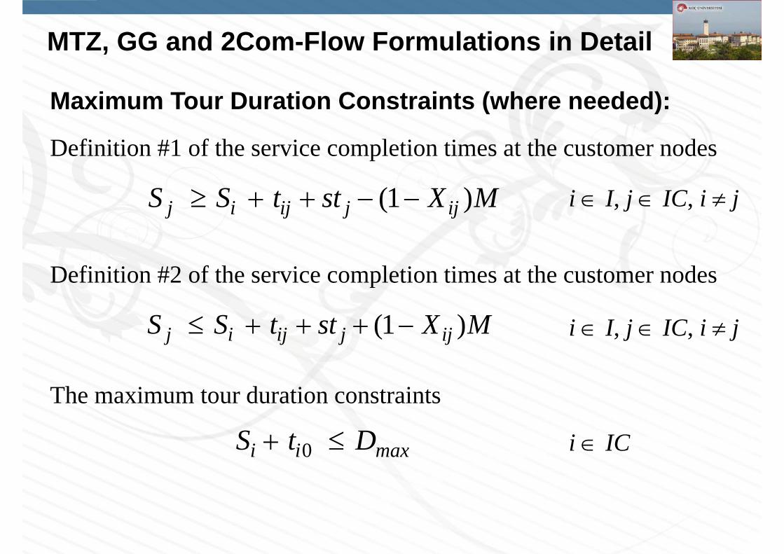
Maximum Tour Duration Constraints (where needed):
Definition #1 of the service completion times at the customer nodes
(1 ) j i ij j ijS S t st X M
(1 ) j i ij j ijS S t st X M
0 i i maxS t D
Definition #2 of the service completion times at the customer nodes
The maximum tour duration constraints
i I, j IC, i j
i I, j IC, i j
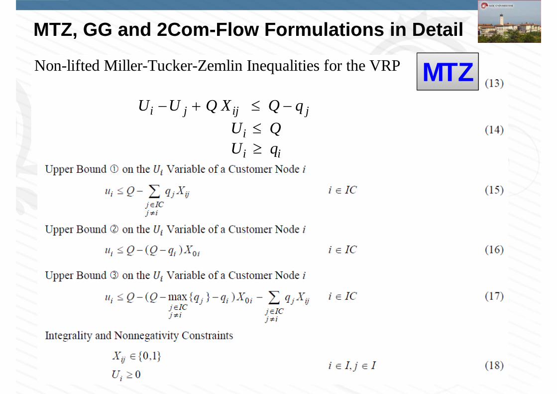
i IC

Ui qi
Ui
qj
MTZ, GG and 2Com-Flow Formulations in Detail
MTZ
i
Xij = 1
qi
Ui
qj
j
MTZ, GG and 2Com-Flow Formulations in Detail
MTZNon-lifted Miller-Tucker-Zemlin Inequalities for the VRP
i j ij j
i
i i
U U Q X Q qU QU q
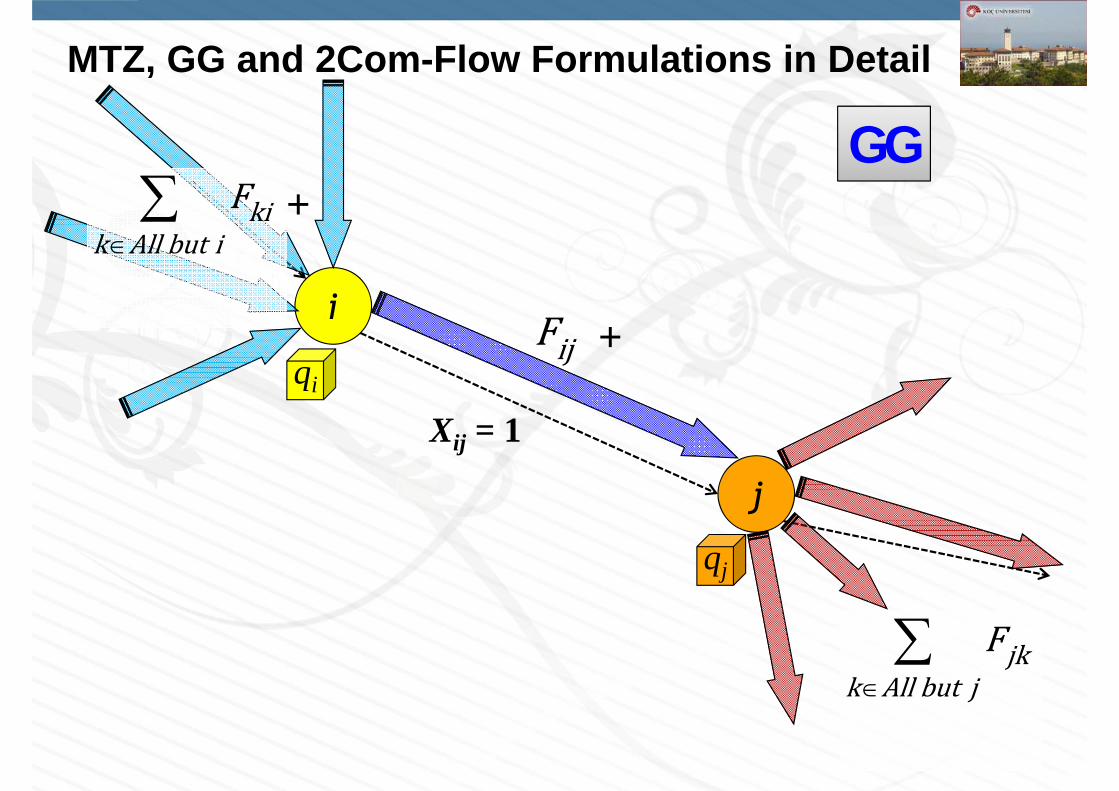
MTZ, GG and 2Com-Flow Formulations in Detail
GG
i
Xij = 1
qj
j
kik All but i
ij
jkk All but j
qi
+
+
MTZ, GG and 2Com-Flow Formulations in Detail
GG
Non-lifted Bounds on the Flow Variables
0
ij
ij
FF Q
, ,
ji i ijj I j i j I j i
F q F i IC
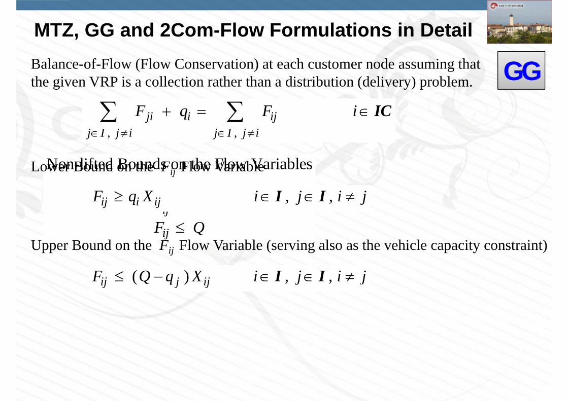
Balance-of-Flow (Flow Conservation) at each customer node assuming that the given VRP is a collection rather than a distribution (delivery) problem.
Lower Bound on the Fij Flow Variable
ij i ijF q X i , j j, iI I
Upper Bound on the Fij Flow Variable (serving also as the vehicle capacity constraint)
( ) ij j ijF Q q X i , j , j iI I
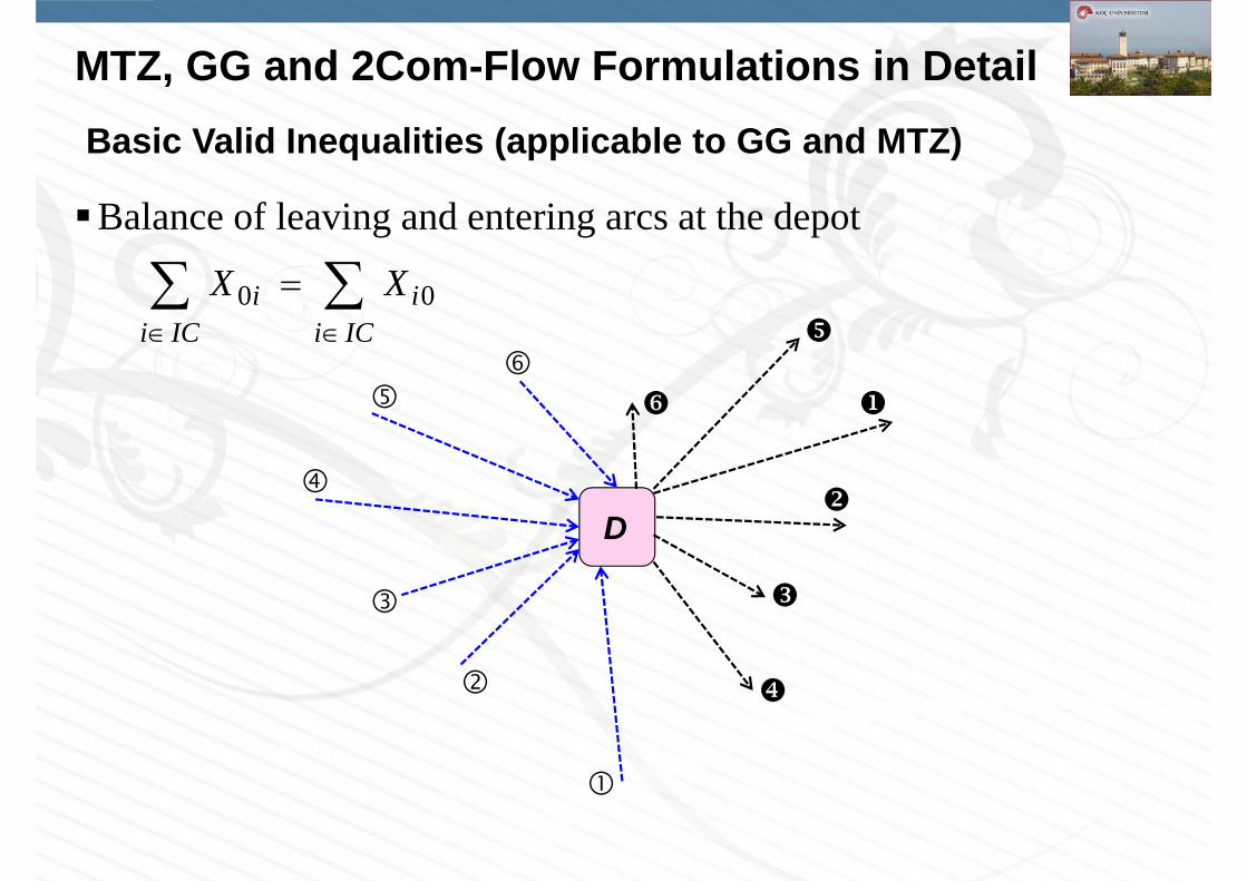
MTZ, GG and 2Com-Flow Formulations in DetailBasic Valid Inequalities (applicable to GG and MTZ)
Balance of leaving and entering arcs at the depot
0 0
i ii IC i IC
X X
D
MTZ, GG and 2Com-Flow Formulations in DetailBasic Valid Inequalities (applicable to GG and MTZ)
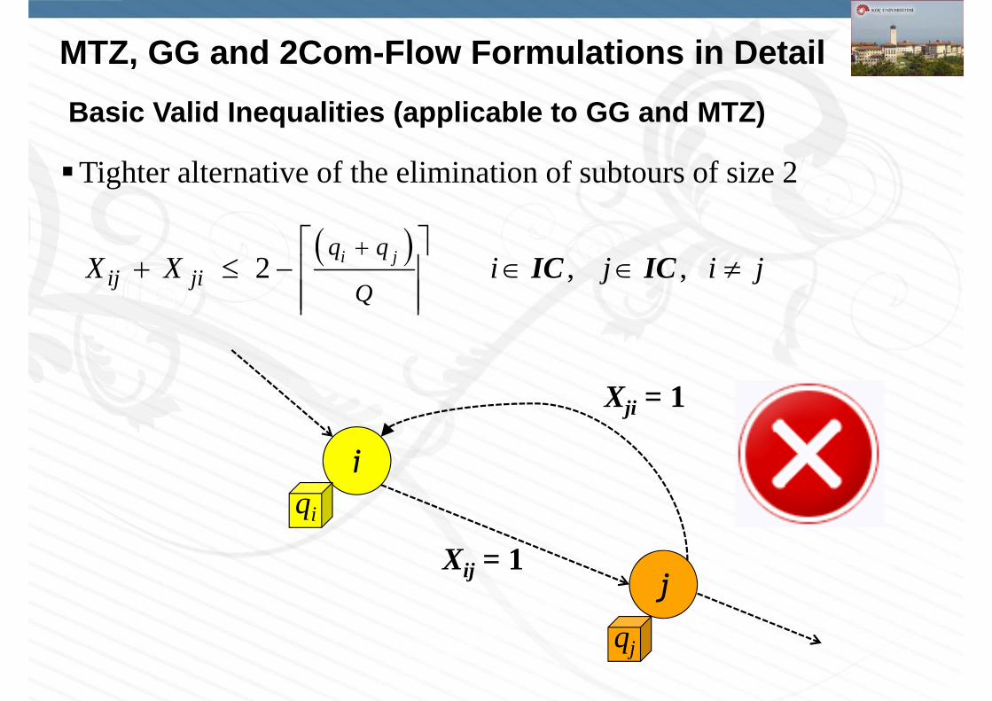
Tighter alternative of the elimination of subtours of size 2
2 , ,
i j
ij jiq q
QX X i j i j IC IC
i
Xij = 1
qi
qj
j
Xji = 1
MTZ, GG and 2Com-Flow Formulations in DetailBasic Valid Inequalities (applicable to GG and MTZ)
Tighter alternative of the elimination of subtours of size 3
3 , , ,
i j k
ij jk kiq q q
QX X X jj k ki iIC IC IC
i
Xij = 1
qi
qj
j
Xki = 1
kXjk = 1qk
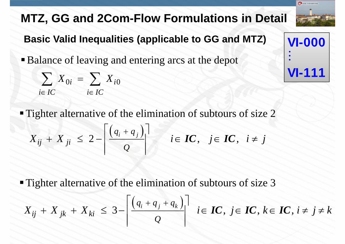
MTZ, GG and 2Com-Flow Formulations in DetailBasic Valid Inequalities (applicable to GG and MTZ) VI-000
VI-111
Balance of leaving and entering arcs at the depot
0 0
i ii IC i IC
X X
Tighter alternative of the elimination of subtours of size 2
2 , ,
i j
ij jiq q
QX X i j i j IC IC
Tighter alternative of the elimination of subtours of size 3
3 , , ,
i j k
ij jk kiq q q
QX X X jj k ki iIC IC IC
MTZ, GG and 2Com-Flow Formulations in Detail
2Com-Flow
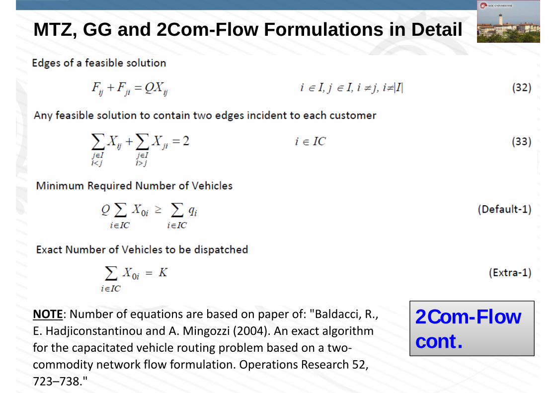
MTZ, GG and 2Com-Flow Formulations in Detail
2Com-Flow cont.
NOTE: Number of equations are based on paper of: "Baldacci, R., E. Hadjiconstantinou and A. Mingozzi (2004). An exact algorithm for the capacitated vehicle routing problem based on a two‐commodity network flow formulation. Operations Research 52, 723–738."
OVERVIEW Introduction and motivation Lifted_MTZ, 1Com-Flow (GG) and 2Com-Flow formulations Experimental setup and results
– Round 1: Gurobi (GRB) and Cplex (CPL) on GG and Lifted_MTZ models of 39 small and medium sized instances
• Effect of the MinNumVec constraint as a valid inequality (VI)
– Round 2: GRB on GG with all VIs and concurrentmip options
– Round 3: GRB_GG with 4 VIs and 2 concurrentmip options on 26 large sized instances
– Round 4: GRB_GG on 8 asymmetric VRPLib instances with 4 VIs
– Round 5: 2Com-Flow formulation on 16 medium sized instances
• Effect of the ExactNumVec constraint as a VI
– Round 6: GRB_GG on 29 XL sized instances with 2 VIs
– Round 7: GRB_GG on 29 XL sized instances with 4 Granular VI Configurations
Conclusion
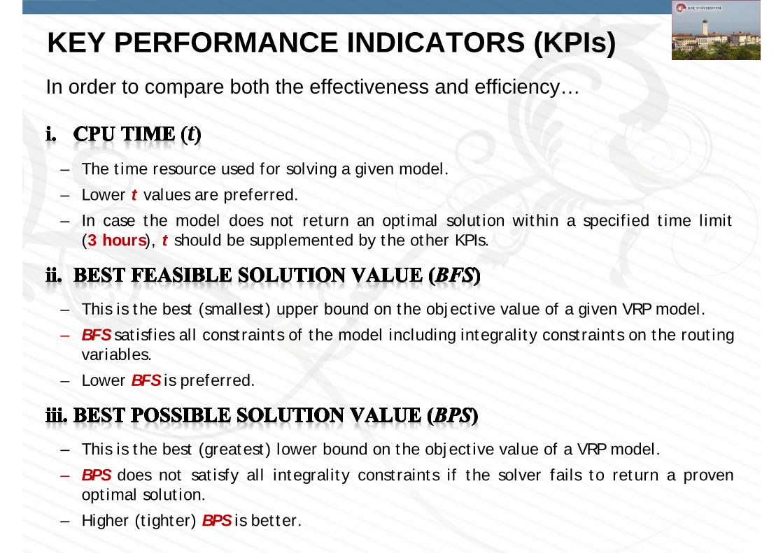
KEY PERFORMANCE INDICATORS (KPIs)In order to compare both the effectiveness and efficiency…
t– The time resource used for solving a given model.
– Lower t values are preferred.
– In case the model does not return an optimal solution within a specified time limit(3 hours), t should be supplemented by the other KPIs.
– This is the best (smallest) upper bound on the objective value of a given VRP model.
– BFS satisfies all constraints of the model including integrality constraints on the routingvariables.
– Lower BFS is preferred.
– This is the best (greatest) lower bound on the objective value of a VRP model.
– BPS does not satisfy all integrality constraints if the solver fails to return a provenoptimal solution.
– Higher (tighter) BPS is better.

KEY PERFORMANCE INDICATORS (KPIs)In order to compare both the effectiveness and efficiency…
– It is computed as (BFSBPS)/BFS100%.
– In a proven optimal VRP solution it will be zero.
– Smaller gap_GAMS values mean better effectiveness.
– It is computed as (BFSBKS)/BKS100% where BKS implies the objective value of the Best Known Solution in the literature.
– Smaller gap_BKS values mean better effectiveness.
in lieu of BFS
in lieu of BPS

READY TO EXPLORE DEEPER!
What do we have?
3 formulations: MTZ, GG, 2Com-Flow
1+3+1 VIs:i. MinNumVec (applicable to all three models)
ii. ExactNumVec (applicable to 2Com-Flow only)
iii. Balance_of_Degree at the depot (applicable to MTZ and GG)
iv. Elimination_of_Subtours_of_size_2 (applicable to MTZ and GG)
v. Elimination_of_Subtours_of_size_3 (applicable to MTZ and GG)
2 solvers: Cplex, Gurobi
• Parallel Computing Options (1 set applicable to both)
• concurrentmip 1 or 2 (applicable to Gurobi only)
– concurrentmip 3 (no marginal gain, yes marginal deterioration!)
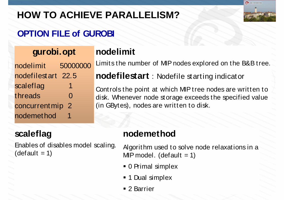
HOW TO ACHIEVE PARALLELISM?
OPTION FILE of GUROBI
gurobi.optnodelimit 50000000nodefilestart 22.5scaleflag 1 threads 0concurrentmip 2nodemethod 1
nodelimitLimits the number of MIP nodes explored on the B&B tree.
nodefilestart : Nodefile starting indicator
Controls the point at which MIP tree nodes are written to disk. Whenever node storage exceeds the specified value (in GBytes), nodes are written to disk.
nodemethodAlgorithm used to solve node relaxations in a MIP model. (default = 1)
0 Primal simplex
1 Dual simplex
2 Barrier
scaleflagEnables of disables model scaling. (default = 1)

HOW TO ACHIEVE PARALLELISM?
OPTION FILE of GUROBI
threads (to be set to 0)Controls the number of threads to apply to parallel MIP or Barrier. Default number of parallel threads allowed for any solution method.
Non-positive values are interpreted as the number of cores to leave free, so setting threads to 0 uses all available cores while setting threads to 1 leaves one core free for other tasks.
concurrentmipThis parameter enables the concurrent MIP solver. When the parameter is set to value n, the MIP solver performs n independent MIP solves in parallel, with different parameter settings for each. Optimization terminates when the first solve completes. Gurobi chooses the parameter settings used for each independent solve automatically.
The intent of concurrent MIP solving is to introduce additional diversity into the MIP search. This approach can sometimes solve models much faster than applying all available threads to a single MIP solve, especially on very large parallel machines.
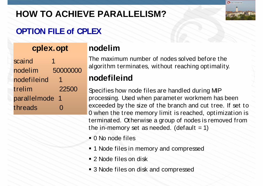
HOW TO ACHIEVE PARALLELISM?
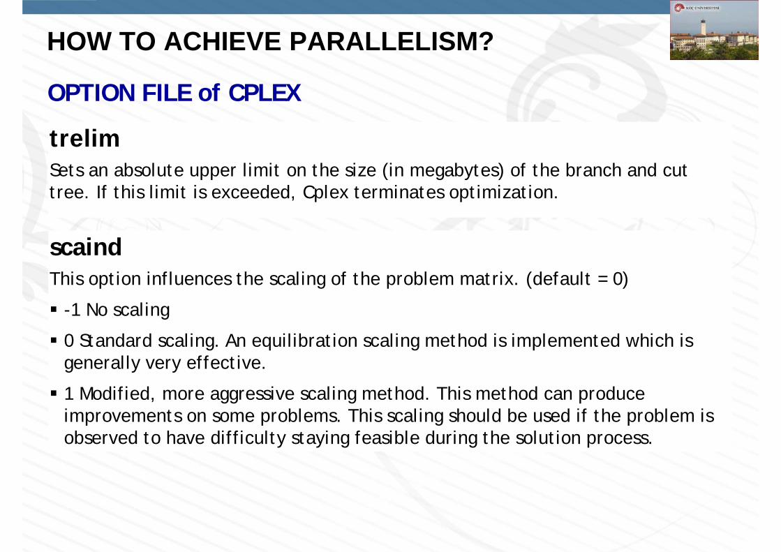
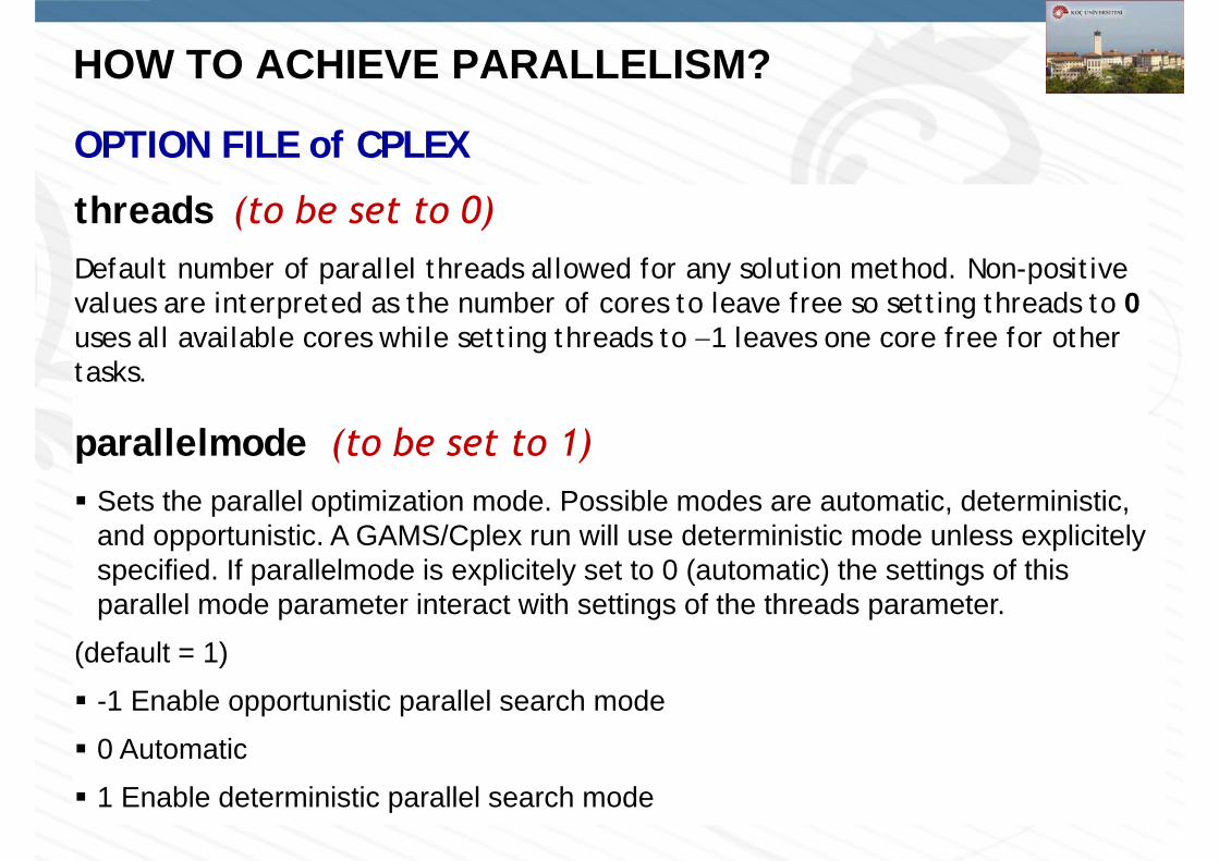
OPTION FILE of CPLEX
cplex.optscaind 1nodelim 50000000nodefileind 1trelim 22500parallelmode 1threads 0
nodelimThe maximum number of nodes solved before the algorithm terminates, without reaching optimality.
nodefileindSpecifies how node files are handled during MIP processing. Used when parameter workmem has been exceeded by the size of the branch and cut tree. If set to 0 when the tree memory limit is reached, optimization is terminated. Otherwise a group of nodes is removed from the in-memory set as needed. (default = 1)
0 No node files
1 Node files in memory and compressed
2 Node files on disk
3 Node files on disk and compressed
HOW TO ACHIEVE PARALLELISM?
OPTION FILE of CPLEX
scaindThis option influences the scaling of the problem matrix. (default = 0)
-1 No scaling
0 Standard scaling. An equilibration scaling method is implemented which is generally very effective.
1 Modified, more aggressive scaling method. This method can produce improvements on some problems. This scaling should be used if the problem is observed to have difficulty staying feasible during the solution process.
trelimSets an absolute upper limit on the size (in megabytes) of the branch and cut tree. If this limit is exceeded, Cplex terminates optimization.
HOW TO ACHIEVE PARALLELISM?
OPTION FILE of CPLEX
threads (to be set to 0)Default number of parallel threads allowed for any solution method. Non-positive values are interpreted as the number of cores to leave free so setting threads to 0uses all available cores while setting threads to 1 leaves one core free for other tasks.
parallelmode (to be set to 1) Sets the parallel optimization mode. Possible modes are automatic, deterministic,
and opportunistic. A GAMS/Cplex run will use deterministic mode unless explicitelyspecified. If parallelmode is explicitely set to 0 (automatic) the settings of this parallel mode parameter interact with settings of the threads parameter.
(default = 1)
-1 Enable opportunistic parallel search mode
0 Automatic
1 Enable deterministic parallel search mode
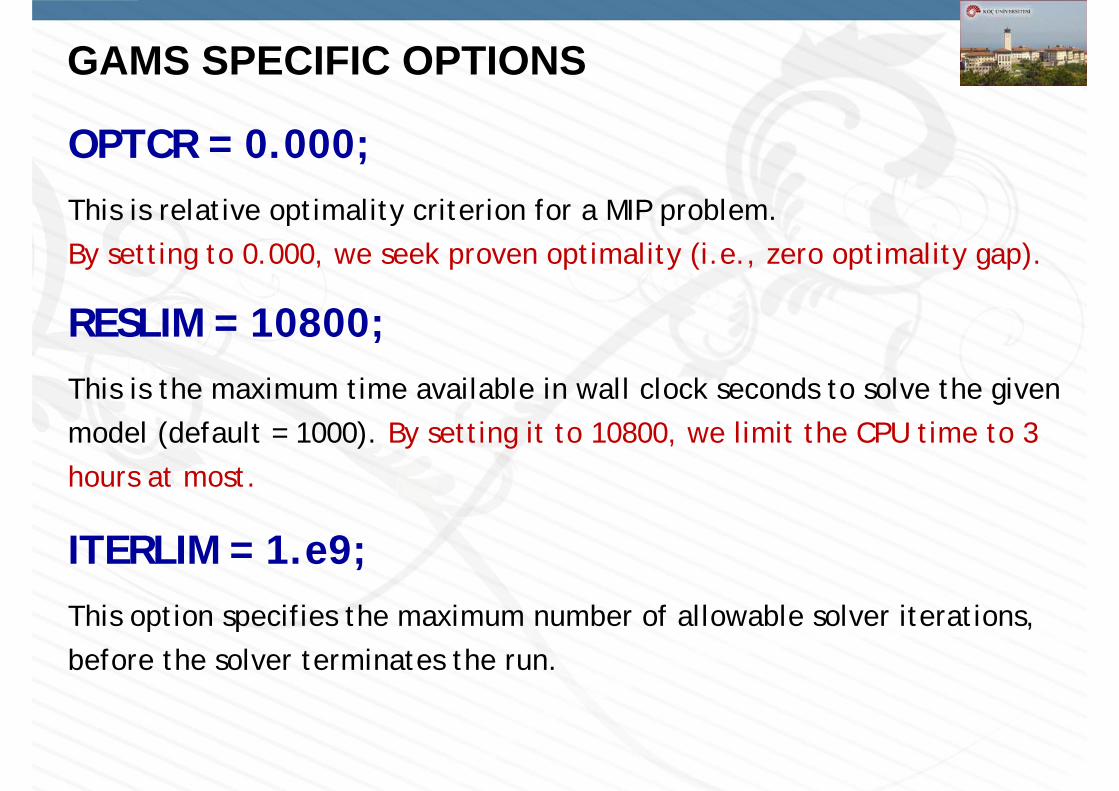
GAMS SPECIFIC OPTIONS
OPTCR = 0.000;This is relative optimality criterion for a MIP problem. By setting to 0.000, we seek proven optimality (i.e., zero optimality gap).
RESLIM = 10800;This is the maximum time available in wall clock seconds to solve the given model (default = 1000). By setting it to 10800, we limit the CPU time to 3 hours at most.
ITERLIM = 1.e9;This option specifies the maximum number of allowable solver iterations, before the solver terminates the run.
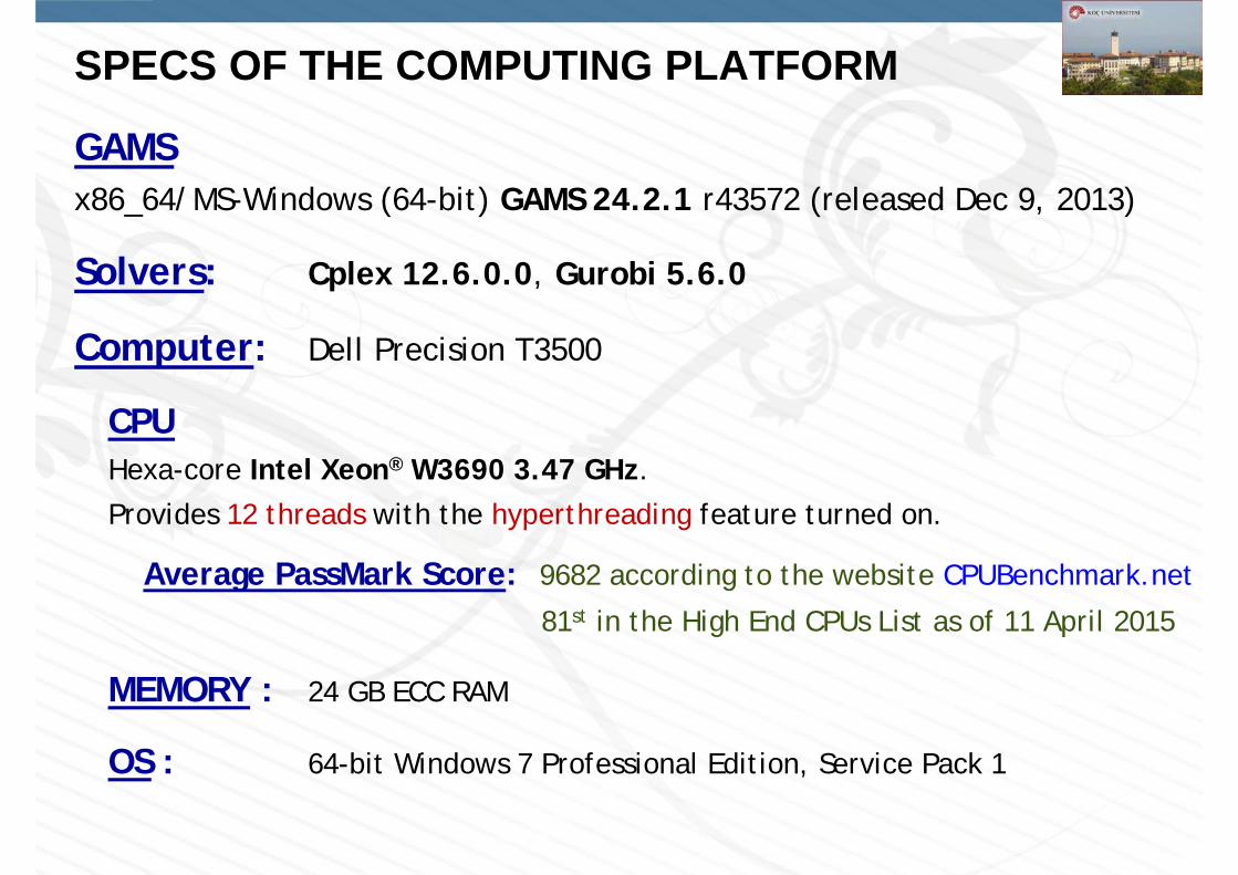
SPECS OF THE COMPUTING PLATFORM
GAMSx86_64/MS-Windows (64-bit) GAMS 24.2.1 r43572 (released Dec 9, 2013)
Solvers: Cplex 12.6.0.0, Gurobi 5.6.0
Computer: Dell Precision T3500
CPUHexa-core Intel Xeon® W3690 3.47 GHz.
Provides 12 threads with the hyperthreading feature turned on.
Average PassMark Score: 9682 according to the website CPUBenchmark.net
81st in the High End CPUs List as of 11 April 2015
MEMORY : 24 GB ECC RAM
OS : 64-bit Windows 7 Professional Edition, Service Pack 1
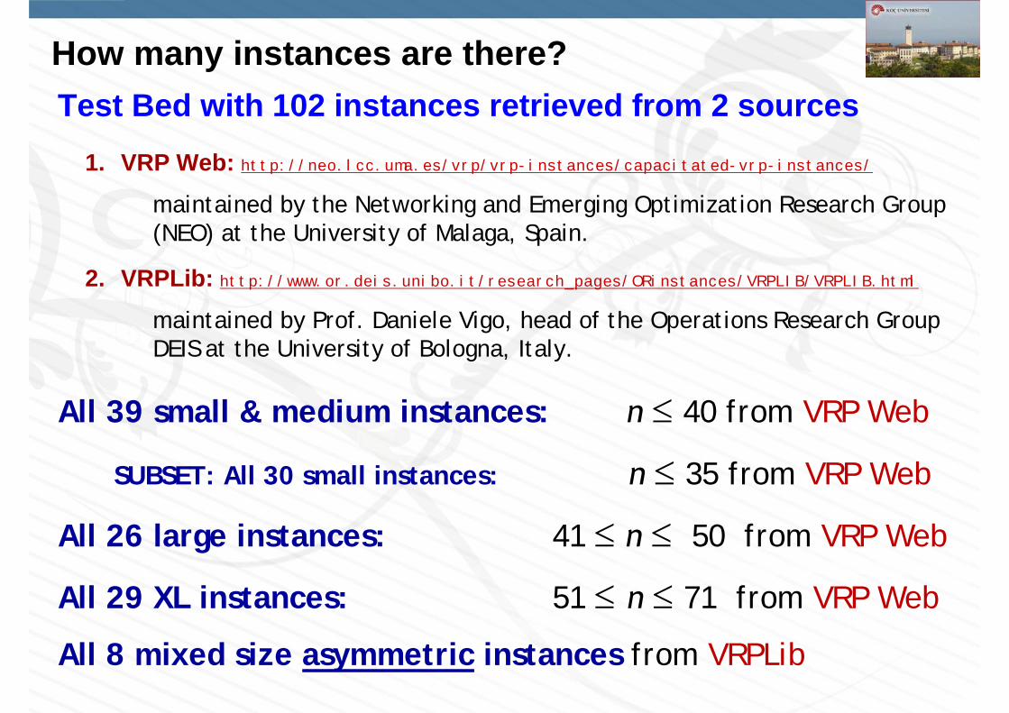
How many instances are there?Test Bed with 102 instances retrieved from 2 sources
1. VRP Web: http://neo.lcc.uma.es/vrp/vrp-instances/capacitated-vrp-instances/
maintained by the Networking and Emerging Optimization Research Group (NEO) at the University of Malaga, Spain.
2. VRPLib: http://www.or.deis.unibo.it/research_pages/ORinstances/VRPLIB/VRPLIB.html
maintained by Prof. Daniele Vigo, head of the Operations Research Group DEIS at the University of Bologna, Italy.
All 39 small & medium instances: n 40 from VRP Web
SUBSET: All 30 small instances: n 35 from VRP Web
All 26 large instances: 41 n 50 from VRP Web
All 29 XL instances: 51 n 71 from VRP Web
All 8 mixed size asymmetric instances from VRPLib
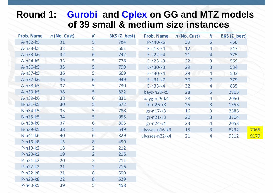
Round 1: Gurobi and Cplex on GG and MTZ models of 39 small & medium size instances
Prob. Name n (No. Cust) K BKS (Z_best)A‐n32‐k5 31 5 784A‐n33‐k5 32 5 661A‐n33‐k6 32 6 742A‐n34‐k5 33 5 778A‐n36‐k5 35 5 799A‐n37‐k5 36 5 669A‐n37‐k6 36 6 949A‐n38‐k5 37 5 730A‐n39‐k5 38 5 822A‐n39‐k6 38 6 831B‐n31‐k5 30 5 672B‐n34‐k5 33 5 788B‐n35‐k5 34 5 955B‐n38‐k6 37 6 805B‐n39‐k5 38 5 549B‐n41‐k6 40 6 829P‐n16‐k8 15 8 450P‐n19‐k2 18 2 212P‐n20‐k2 19 2 216P‐n21‐k2 20 2 211P‐n22‐k2 21 2 216P‐n22‐k8 21 8 590P‐n23‐k8 22 8 529P‐n40‐k5 39 5 458
Prob. Name n (No. Cust) K BKS (Z_best)P‐n40‐k5 39 5 458E‐n13‐k4 12 4 247E‐n22‐k4 21 4 375E‐n23‐k3 22 3 569E‐n30‐k3 29 3 534E‐n30‐k4 29 4 503E‐n31‐k7 30 7 379E‐n33‐k4 32 4 835
bays‐n29‐k5 28 5 2963bayg‐n29‐k4 28 4 2050fri‐n26‐k3 25 3 1353gr‐n17‐k3 16 3 2685gr‐n21‐k3 20 3 3704gr‐n24‐k4 23 4 2053
ulysses‐n16‐k3 15 3 8232 7965ulysses‐n22‐k4 21 4 9312 9179
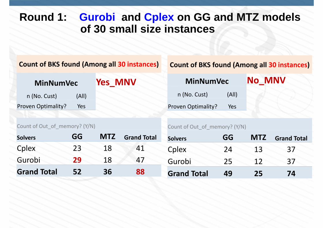
Round 1: Gurobi and Cplex on GG and MTZ models of 30 small size instances
Count of BKS found (Among all 30 instances)
MinNumVec Yes_MNVn (No. Cust) (All)
Proven Optimality? Yes
Count of Out_of_memory? (Y/N)
Solvers GG MTZ Grand Total
Cplex 23 18 41Gurobi 29 18 47Grand Total 52 36 88
Count of BKS found (Among all 30 instances)
MinNumVec No_MNVn (No. Cust) (All)
Proven Optimality? Yes
Count of Out_of_memory? (Y/N)
Solvers GG MTZ Grand Total
Cplex 24 13 37Gurobi 25 12 37Grand Total 49 25 74
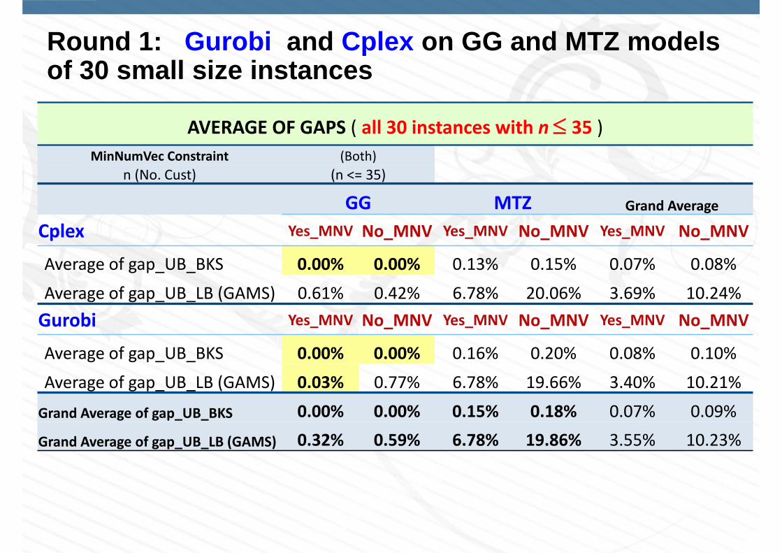
Round 1: Gurobi and Cplex on GG and MTZ models of 30 small size instances
AVERAGE OF GAPS ( all 30 instances with n 35 )MinNumVec Constraint (Both)
n (No. Cust) (n <= 35)
GG MTZ Grand Average
Cplex Yes_MNV No_MNV Yes_MNV No_MNV Yes_MNV No_MNV
Average of gap_UB_BKS 0.00% 0.00% 0.13% 0.15% 0.07% 0.08%
Average of gap_UB_LB (GAMS) 0.61% 0.42% 6.78% 20.06% 3.69% 10.24%Gurobi Yes_MNV No_MNV Yes_MNV No_MNV Yes_MNV No_MNV
Average of gap_UB_BKS 0.00% 0.00% 0.16% 0.20% 0.08% 0.10%
Average of gap_UB_LB (GAMS) 0.03% 0.77% 6.78% 19.66% 3.40% 10.21%
Grand Average of gap_UB_BKS 0.00% 0.00% 0.15% 0.18% 0.07% 0.09%
Grand Average of gap_UB_LB (GAMS) 0.32% 0.59% 6.78% 19.86% 3.55% 10.23%

Round 1: Gurobi and Cplex on GG and MTZ models of 30 small size instances
CPU TIME ANALYSES ( all 30 instances with n 35 )MinNumVec Constraint (Both)
n (No. Cust) (n <= 35)
GG MTZ Grand Average
Cplex Yes_MNV No_MNV Yes_MNV No_MNV Yes_MNV No_MNV
Average of CPU (s) 2,545 2,401 4,440 6,104 3,492 4,253
Gurobi Yes_MNV No_MNV Yes_MNV No_MNV Yes_MNV No_MNV
Average of CPU (s) 429 1,926 4,869 7,651 2,649 4,789
Grand Average of CPU (s) 1,487 2,164 4,654 6,878 3,071 4,521
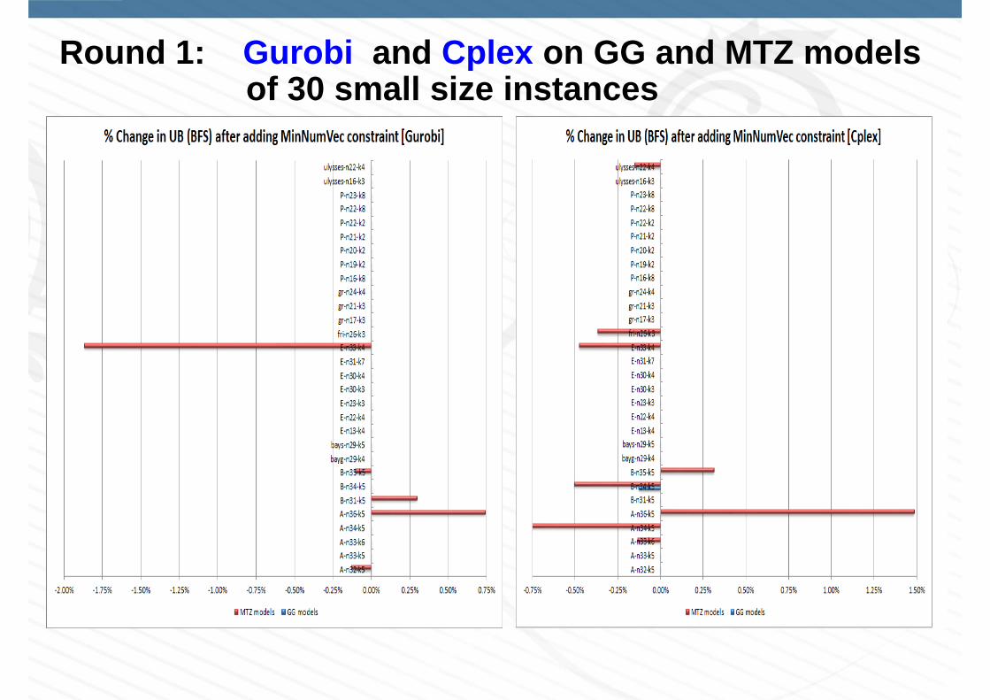
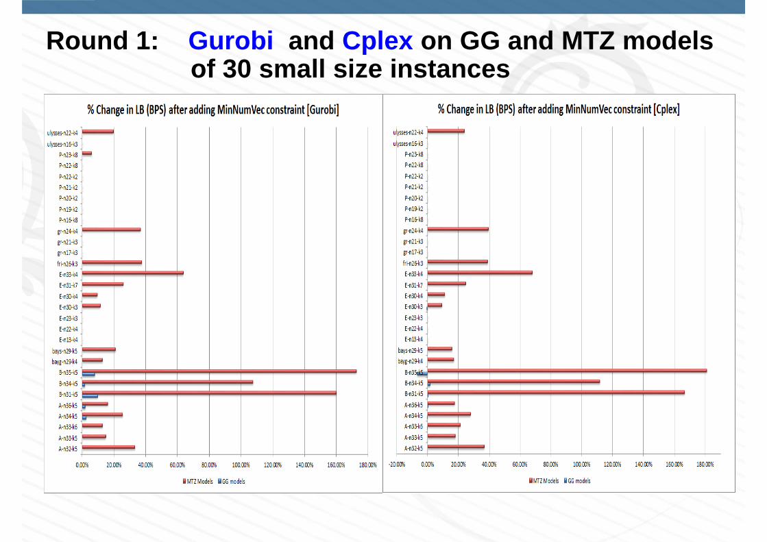
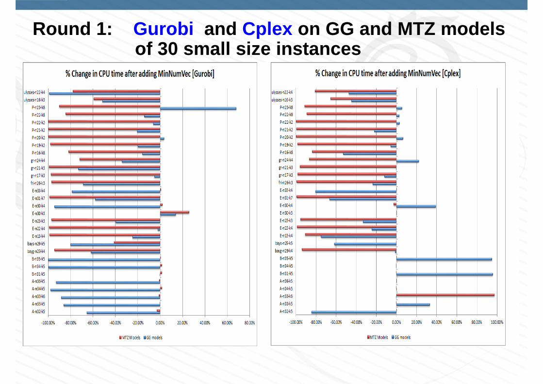
Round 1: Gurobi and Cplex on GG and MTZ models of 30 small size instances
Round 1: Gurobi and Cplex on GG and MTZ models of 30 small size instances
Round 1: Gurobi and Cplex on GG and MTZ models of 30 small size instances
Round 1: Gurobi and Cplex on GG and MTZ models of 39 small & medium size instances
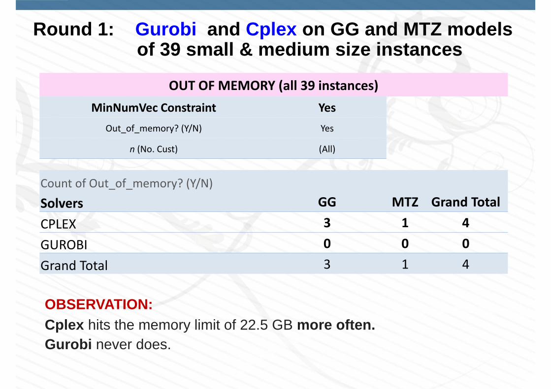
OUT OF MEMORY (all 39 instances)MinNumVec Constraint Yes
Out_of_memory? (Y/N) Yes
n (No. Cust) (All)
Count of Out_of_memory? (Y/N)
Solvers GG MTZ Grand TotalCPLEX 3 1 4GUROBI 0 0 0Grand Total 3 1 4
OBSERVATION:Cplex hits the memory limit of 22.5 GB more often. Gurobi never does.
Round 1: Gurobi and Cplex on GG and MTZ models of 39 small & medium size instances
MinNumVec Constraint : Present Instances : All 39 instances
GG is better than MTZ MTZ is better than GG
gap_UB_BKS gap_GAMS CPU time gap_UB_BKS gap_GAMS CPU time
Cplex 11 21 27 0 0 12
Gurobi 13 21 37 0 0 2
Total 24 42 64 0 0 14
MinNumVec Constraint : Present Instances : All 39 instances
Gurobi is better than Cplex Cplex is better than Gurobi
gap_UB_BKS gap_GAMS CPU time gap_UB_BKS gap_GAMS CPU time
GG 3 14 31 0 0 8
MTZ 4 8 2 6 13 37
Total 7 22 33 6 13 45
WHO IS BETTER?
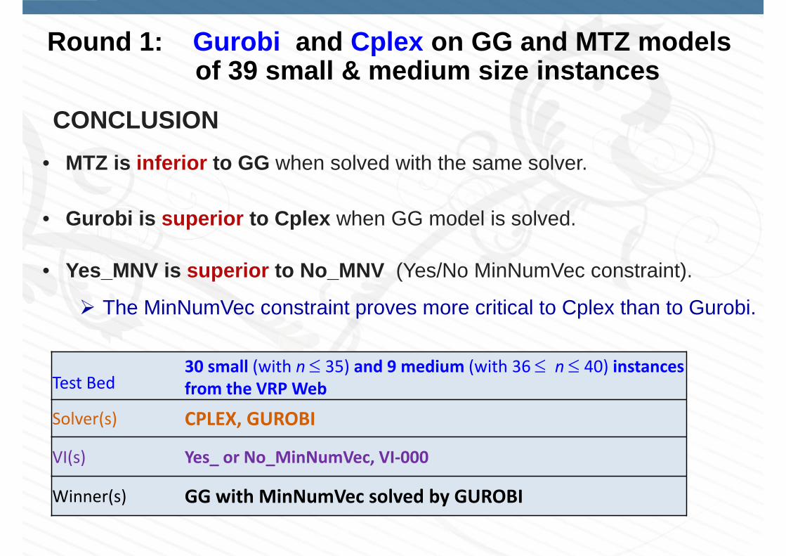
• MTZ is inferior to GG when solved with the same solver.
• Gurobi is superior to Cplex when GG model is solved.
• Yes_MNV is superior to No_MNV (Yes/No MinNumVec constraint).
The MinNumVec constraint proves more critical to Cplex than to Gurobi.
Test Bed30 small (with n 35) and 9 medium (with 36 n 40) instances from the VRP Web
Solver(s) CPLEX, GUROBI
VI(s) Yes_ or No_MinNumVec, VI‐000
Winner(s) GG with MinNumVec solved by GUROBI
CONCLUSION
Round 1: Gurobi and Cplex on GG and MTZ models of 39 small & medium size instances
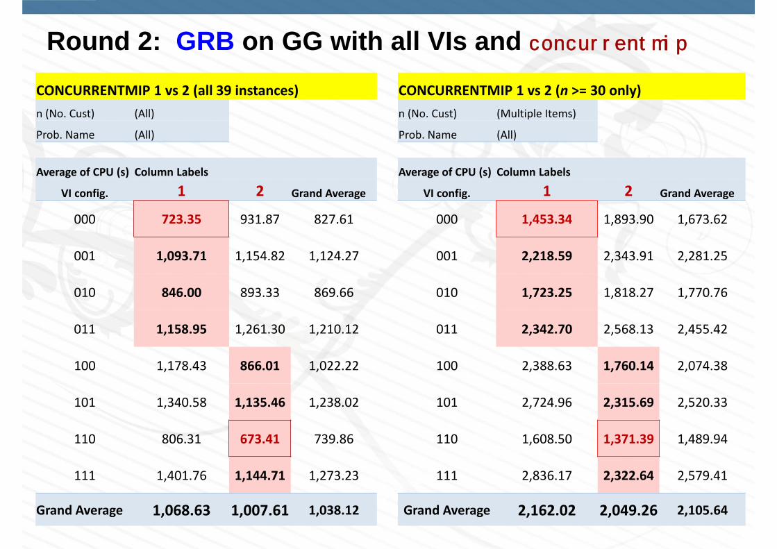
Round 2: GRB on GG with all VIs and concurrentmipCONCURRENTMIP 1 vs 2 (all 39 instances) CONCURRENTMIP 1 vs 2 (n >= 30 only)n (No. Cust) (All) n (No. Cust) (Multiple Items)
Prob. Name (All) Prob. Name (All)
Average of CPU (s) Column Labels Average of CPU (s) Column Labels
VI config. 1 2 Grand Average VI config. 1 2 Grand Average
000 723.35 931.87 827.61 000 1,453.34 1,893.90 1,673.62
001 1,093.71 1,154.82 1,124.27 001 2,218.59 2,343.91 2,281.25
010 846.00 893.33 869.66 010 1,723.25 1,818.27 1,770.76
011 1,158.95 1,261.30 1,210.12 011 2,342.70 2,568.13 2,455.42
100 1,178.43 866.01 1,022.22 100 2,388.63 1,760.14 2,074.38
101 1,340.58 1,135.46 1,238.02 101 2,724.96 2,315.69 2,520.33
110 806.31 673.41 739.86 110 1,608.50 1,371.39 1,489.94
111 1,401.76 1,144.71 1,273.23 111 2,836.17 2,322.64 2,579.41
Grand Average 1,068.63 1,007.61 1,038.12 Grand Average 2,162.02 2,049.26 2,105.64
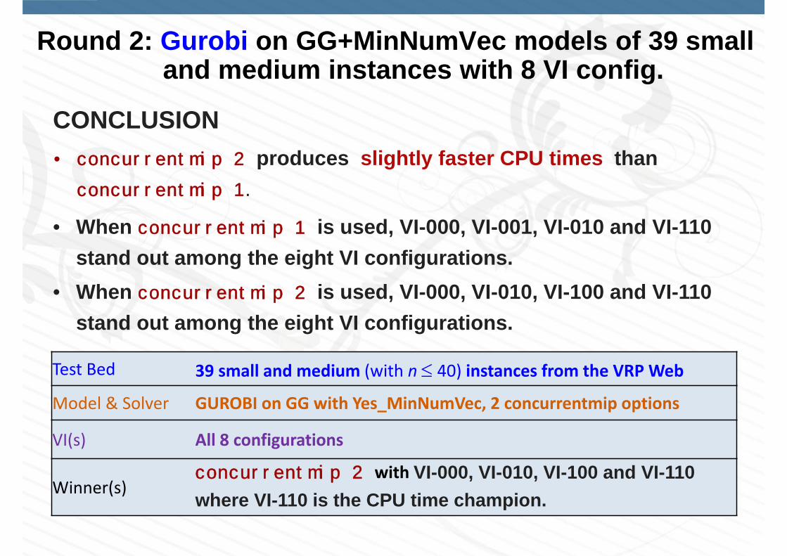
Round 2: Gurobi on GG+MinNumVec models of 39 small and medium instances with 8 VI config.
• concurrentmip 2 produces slightly faster CPU times than concurrentmip 1.
• When concurrentmip 1 is used, VI-000, VI-001, VI-010 and VI-110stand out among the eight VI configurations.
• When concurrentmip 2 is used, VI-000, VI-010, VI-100 and VI-110stand out among the eight VI configurations.
Test Bed 39 small and medium (with n 40) instances from the VRP Web
Model & Solver GUROBI on GG with Yes_MinNumVec, 2 concurrentmip options
VI(s) All 8 configurations
Winner(s)concurrentmip 2 with VI-000, VI-010, VI-100 and VI-110where VI-110 is the CPU time champion.
CONCLUSION
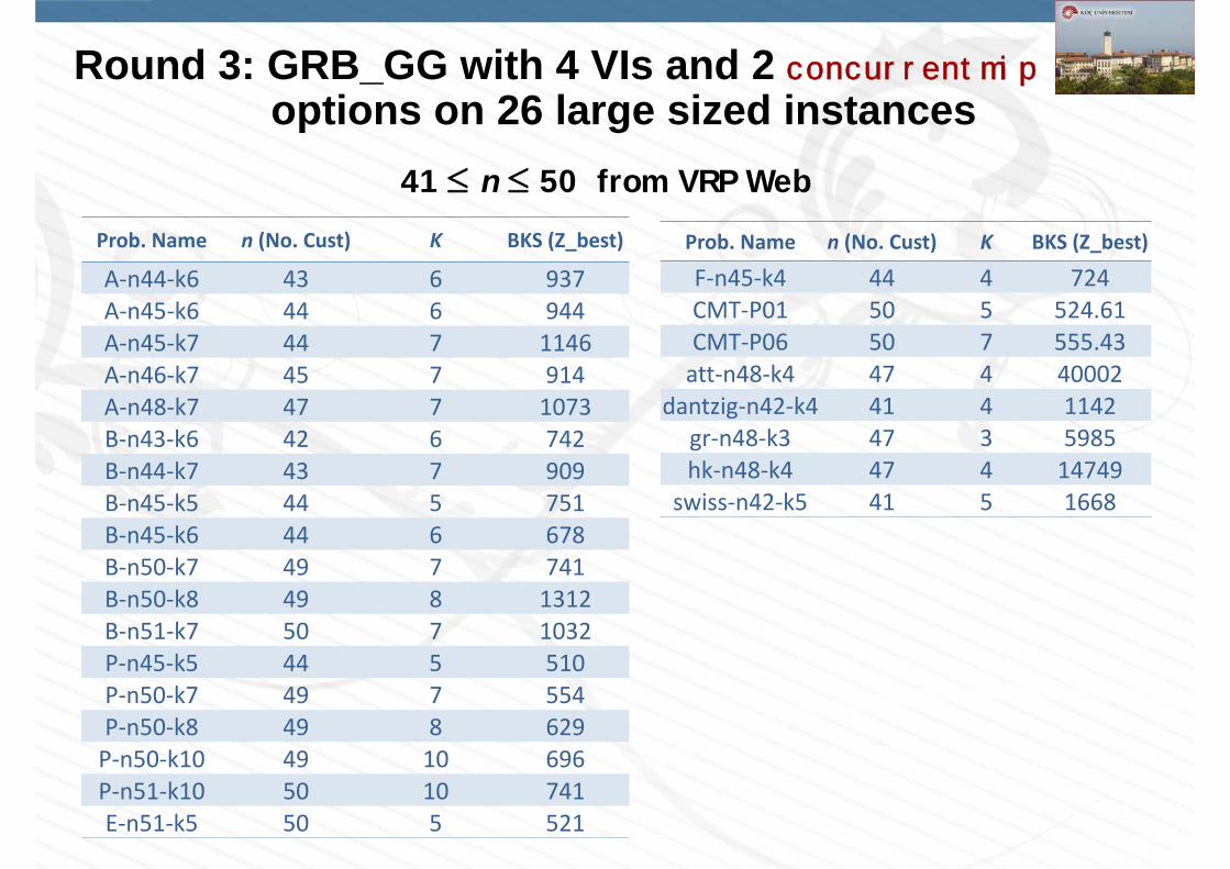
Round 3: GRB_GG with 4 VIs and 2 concurrentmipoptions on 26 large sized instances
Prob. Name n (No. Cust) K BKS (Z_best)
A‐n44‐k6 43 6 937A‐n45‐k6 44 6 944A‐n45‐k7 44 7 1146A‐n46‐k7 45 7 914A‐n48‐k7 47 7 1073B‐n43‐k6 42 6 742B‐n44‐k7 43 7 909B‐n45‐k5 44 5 751B‐n45‐k6 44 6 678B‐n50‐k7 49 7 741B‐n50‐k8 49 8 1312B‐n51‐k7 50 7 1032P‐n45‐k5 44 5 510P‐n50‐k7 49 7 554P‐n50‐k8 49 8 629P‐n50‐k10 49 10 696P‐n51‐k10 50 10 741E‐n51‐k5 50 5 521
Prob. Name n (No. Cust) K BKS (Z_best)
F‐n45‐k4 44 4 724CMT‐P01 50 5 524.61CMT‐P06 50 7 555.43att‐n48‐k4 47 4 40002
dantzig‐n42‐k4 41 4 1142gr‐n48‐k3 47 3 5985hk‐n48‐k4 47 4 14749
swiss‐n42‐k5 41 5 1668
41 n 50 from VRP Web
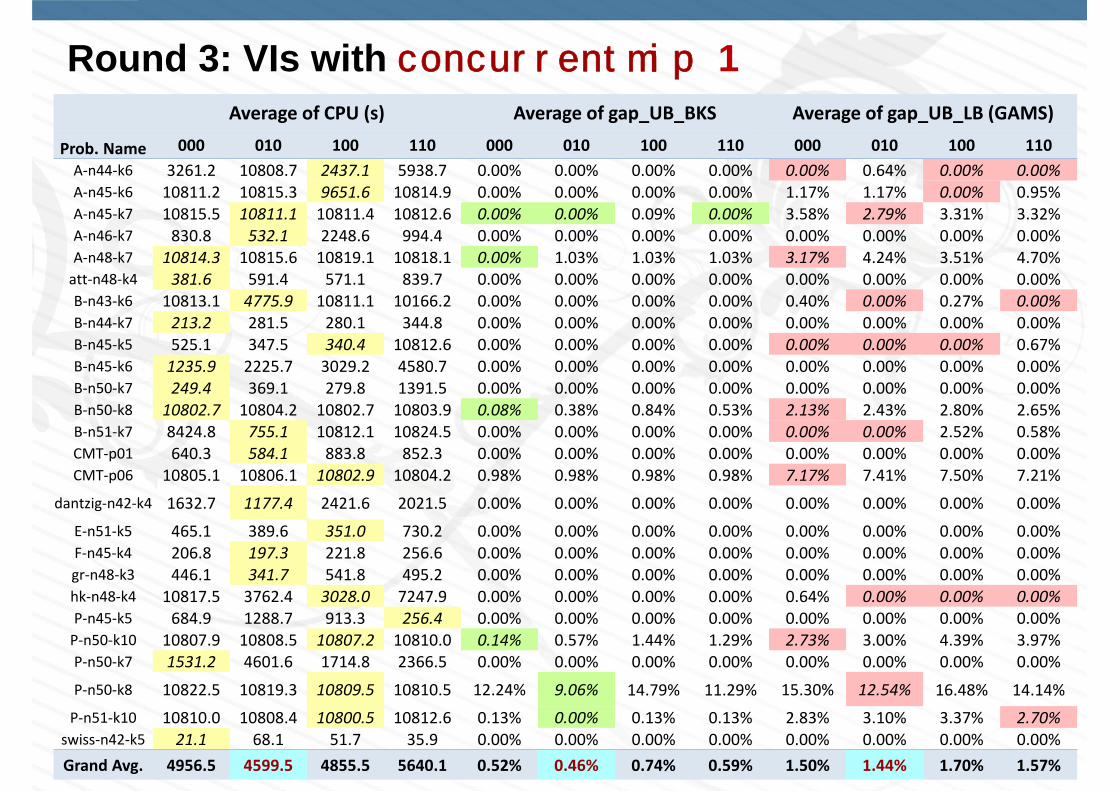
Round 3: VIs with concurrentmip 1Average of CPU (s) Average of gap_UB_BKS Average of gap_UB_LB (GAMS)
Prob. Name 000 010 100 110 000 010 100 110 000 010 100 110A‐n44‐k6 3261.2 10808.7 2437.1 5938.7 0.00% 0.00% 0.00% 0.00% 0.00% 0.64% 0.00% 0.00%A‐n45‐k6 10811.2 10815.3 9651.6 10814.9 0.00% 0.00% 0.00% 0.00% 1.17% 1.17% 0.00% 0.95%A‐n45‐k7 10815.5 10811.1 10811.4 10812.6 0.00% 0.00% 0.09% 0.00% 3.58% 2.79% 3.31% 3.32%A‐n46‐k7 830.8 532.1 2248.6 994.4 0.00% 0.00% 0.00% 0.00% 0.00% 0.00% 0.00% 0.00%A‐n48‐k7 10814.3 10815.6 10819.1 10818.1 0.00% 1.03% 1.03% 1.03% 3.17% 4.24% 3.51% 4.70%att‐n48‐k4 381.6 591.4 571.1 839.7 0.00% 0.00% 0.00% 0.00% 0.00% 0.00% 0.00% 0.00%B‐n43‐k6 10813.1 4775.9 10811.1 10166.2 0.00% 0.00% 0.00% 0.00% 0.40% 0.00% 0.27% 0.00%B‐n44‐k7 213.2 281.5 280.1 344.8 0.00% 0.00% 0.00% 0.00% 0.00% 0.00% 0.00% 0.00%B‐n45‐k5 525.1 347.5 340.4 10812.6 0.00% 0.00% 0.00% 0.00% 0.00% 0.00% 0.00% 0.67%B‐n45‐k6 1235.9 2225.7 3029.2 4580.7 0.00% 0.00% 0.00% 0.00% 0.00% 0.00% 0.00% 0.00%B‐n50‐k7 249.4 369.1 279.8 1391.5 0.00% 0.00% 0.00% 0.00% 0.00% 0.00% 0.00% 0.00%B‐n50‐k8 10802.7 10804.2 10802.7 10803.9 0.08% 0.38% 0.84% 0.53% 2.13% 2.43% 2.80% 2.65%B‐n51‐k7 8424.8 755.1 10812.1 10824.5 0.00% 0.00% 0.00% 0.00% 0.00% 0.00% 2.52% 0.58%CMT‐p01 640.3 584.1 883.8 852.3 0.00% 0.00% 0.00% 0.00% 0.00% 0.00% 0.00% 0.00%CMT‐p06 10805.1 10806.1 10802.9 10804.2 0.98% 0.98% 0.98% 0.98% 7.17% 7.41% 7.50% 7.21%
dantzig‐n42‐k4 1632.7 1177.4 2421.6 2021.5 0.00% 0.00% 0.00% 0.00% 0.00% 0.00% 0.00% 0.00%
E‐n51‐k5 465.1 389.6 351.0 730.2 0.00% 0.00% 0.00% 0.00% 0.00% 0.00% 0.00% 0.00%F‐n45‐k4 206.8 197.3 221.8 256.6 0.00% 0.00% 0.00% 0.00% 0.00% 0.00% 0.00% 0.00%gr‐n48‐k3 446.1 341.7 541.8 495.2 0.00% 0.00% 0.00% 0.00% 0.00% 0.00% 0.00% 0.00%hk‐n48‐k4 10817.5 3762.4 3028.0 7247.9 0.00% 0.00% 0.00% 0.00% 0.64% 0.00% 0.00% 0.00%P‐n45‐k5 684.9 1288.7 913.3 256.4 0.00% 0.00% 0.00% 0.00% 0.00% 0.00% 0.00% 0.00%P‐n50‐k10 10807.9 10808.5 10807.2 10810.0 0.14% 0.57% 1.44% 1.29% 2.73% 3.00% 4.39% 3.97%P‐n50‐k7 1531.2 4601.6 1714.8 2366.5 0.00% 0.00% 0.00% 0.00% 0.00% 0.00% 0.00% 0.00%
P‐n50‐k8 10822.5 10819.3 10809.5 10810.5 12.24% 9.06% 14.79% 11.29% 15.30% 12.54% 16.48% 14.14%P‐n51‐k10 10810.0 10808.4 10800.5 10812.6 0.13% 0.00% 0.13% 0.13% 2.83% 3.10% 3.37% 2.70%
swiss‐n42‐k5 21.1 68.1 51.7 35.9 0.00% 0.00% 0.00% 0.00% 0.00% 0.00% 0.00% 0.00%Grand Avg. 4956.5 4599.5 4855.5 5640.1 0.52% 0.46% 0.74% 0.59% 1.50% 1.44% 1.70% 1.57%

Round 3: VIs with concurrentmip 2Average of CPU (s) Average of gap_UB_BKS Average of gap_UB_LB (GAMS)
Prob. Name 000 010 100 110 000 010 100 110 000 010 100 110A‐n44‐k6 9838.8 4268.4 6785.8 6027.3 0.00% 0.00% 0.00% 0.00% 0.00% 0.00% 0.00% 0.00%A‐n45‐k6 10815.1 9875.2 10816.0 10823.6 0.00% 0.00% 0.00% 0.42% 0.95% 0.00% 0.74% 2.11%A‐n45‐k7 10812.6 10816.8 10815.9 10816.6 0.00% 0.00% 0.00% 0.00% 3.14% 3.32% 3.32% 3.66%A‐n46‐k7 1281.3 4129.6 1118.6 646.4 0.00% 0.00% 0.00% 0.00% 0.00% 0.00% 0.00% 0.00%A‐n48‐k7 10827.5 10822.6 10824.8 10820.8 1.03% 1.96% 0.00% 0.00% 3.87% 5.21% 2.70% 3.73%att‐n48‐k4 653.3 724.9 840.8 1296.8 0.00% 0.00% 0.00% 0.00% 0.00% 0.00% 0.00% 0.00%B‐n43‐k6 10814.0 3950.4 2381.1 2893.1 0.00% 0.00% 0.00% 0.00% 0.27% 0.00% 0.00% 0.00%B‐n44‐k7 261.5 333.0 316.0 252.8 0.00% 0.00% 0.00% 0.00% 0.00% 0.00% 0.00% 0.00%B‐n45‐k5 635.5 479.6 406.2 747.2 0.00% 0.00% 0.00% 0.00% 0.00% 0.00% 0.00% 0.00%B‐n45‐k6 5934.8 6070.0 4281.1 5030.6 0.00% 0.00% 0.00% 0.00% 0.00% 0.00% 0.00% 0.00%B‐n50‐k7 254.4 287.3 299.5 333.1 0.00% 0.00% 0.00% 0.00% 0.00% 0.00% 0.00% 0.00%B‐n50‐k8 10804.7 10808.7 10804.2 10805.3 0.23% 0.46% 0.08% 0.00% 2.43% 2.58% 2.06% 2.13%B‐n51‐k7 535.7 3126.1 3809.5 10814.2 0.00% 0.00% 0.00% 0.00% 0.00% 0.00% 0.00% 0.48%CMT‐p01 1067.5 903.5 1173.9 550.4 0.00% 0.00% 0.00% 0.00% 0.00% 0.00% 0.00% 0.00%CMT‐p06 10805.2 10805.4 10804.9 10804.4 0.00% 0.00% 0.98% 0.00% 6.50% 6.62% 7.54% 6.35%
dantzig‐n42‐k4 2368.8 1798.8 1898.0 1984.5 0.00% 0.00% 0.00% 0.00% 0.00% 0.00% 0.00% 0.00%
E‐n51‐k5 527.7 936.8 799.9 546.6 0.00% 0.00% 0.00% 0.00% 0.00% 0.00% 0.00% 0.00%F‐n45‐k4 188.8 182.1 169.3 118.5 0.00% 0.00% 0.00% 0.00% 0.00% 0.00% 0.00% 0.00%gr‐n48‐k3 573.4 313.4 767.4 515.3 0.00% 0.00% 0.00% 0.00% 0.00% 0.00% 0.00% 0.00%hk‐n48‐k4 2695.4 6854.7 1462.2 10820.6 0.00% 0.00% 0.00% 0.00% 0.00% 0.00% 0.00% 1.15%P‐n45‐k5 390.1 903.7 356.2 1169.0 0.00% 0.00% 0.00% 0.00% 0.00% 0.00% 0.00% 0.00%P‐n50‐k10 10807.6 10817.6 10810.6 10814.1 0.57% 0.86% 0.14% 1.58% 3.43% 3.85% 3.01% 4.81%P‐n50‐k7 3466.0 2468.1 3989.0 3902.5 0.00% 0.00% 0.00% 0.00% 0.00% 0.00% 0.00% 0.00%
P‐n50‐k8 10820.0 10812.6 10815.2 10820.6 4.77% 3.18% 9.06% 4.77% 8.80% 7.55% 12.24% 8.80%
P‐n51‐k10 10810.4 10813.6 10806.7 10814.0 0.00% 0.13% 1.35% 1.21% 2.97% 3.10% 4.53% 4.27%swiss‐n42‐k5 29.5 58.6 45.2 51.1 0.00% 0.00% 0.00% 0.00% 0.00% 0.00% 0.00% 0.00%Grand Avg. 4923.8 4744.7 4515.3 5162.3 0.25% 0.25% 0.45% 0.31% 1.24% 1.24% 1.39% 1.44%
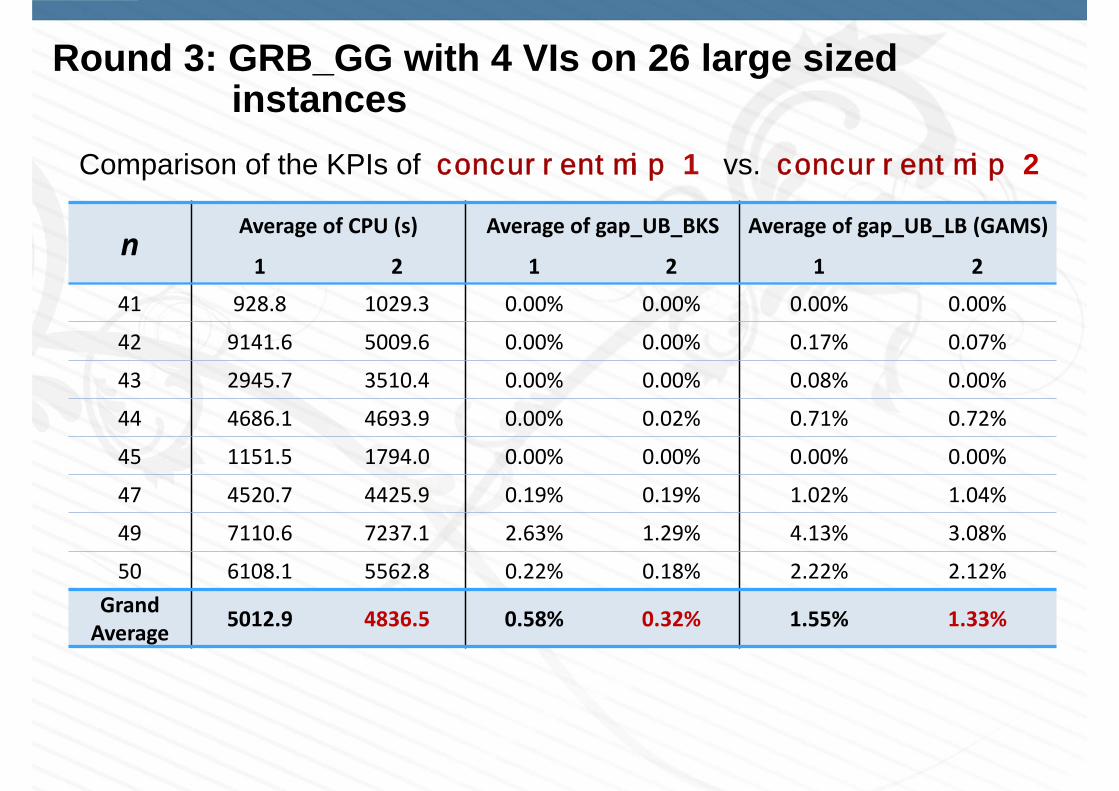
Round 3: GRB_GG with 4 VIs on 26 large sized instances
nAverage of CPU (s) Average of gap_UB_BKS Average of gap_UB_LB (GAMS)
1 2 1 2 1 2
41 928.8 1029.3 0.00% 0.00% 0.00% 0.00%
42 9141.6 5009.6 0.00% 0.00% 0.17% 0.07%
43 2945.7 3510.4 0.00% 0.00% 0.08% 0.00%
44 4686.1 4693.9 0.00% 0.02% 0.71% 0.72%
45 1151.5 1794.0 0.00% 0.00% 0.00% 0.00%
47 4520.7 4425.9 0.19% 0.19% 1.02% 1.04%
49 7110.6 7237.1 2.63% 1.29% 4.13% 3.08%
50 6108.1 5562.8 0.22% 0.18% 2.22% 2.12%Grand Average 5012.9 4836.5 0.58% 0.32% 1.55% 1.33%
Comparison of the KPIs of concurrentmip 1 vs. concurrentmip 2
Round 3: GRB_GG with 4 VIs and 2 concurrentmipoptions on 26 large sized instances
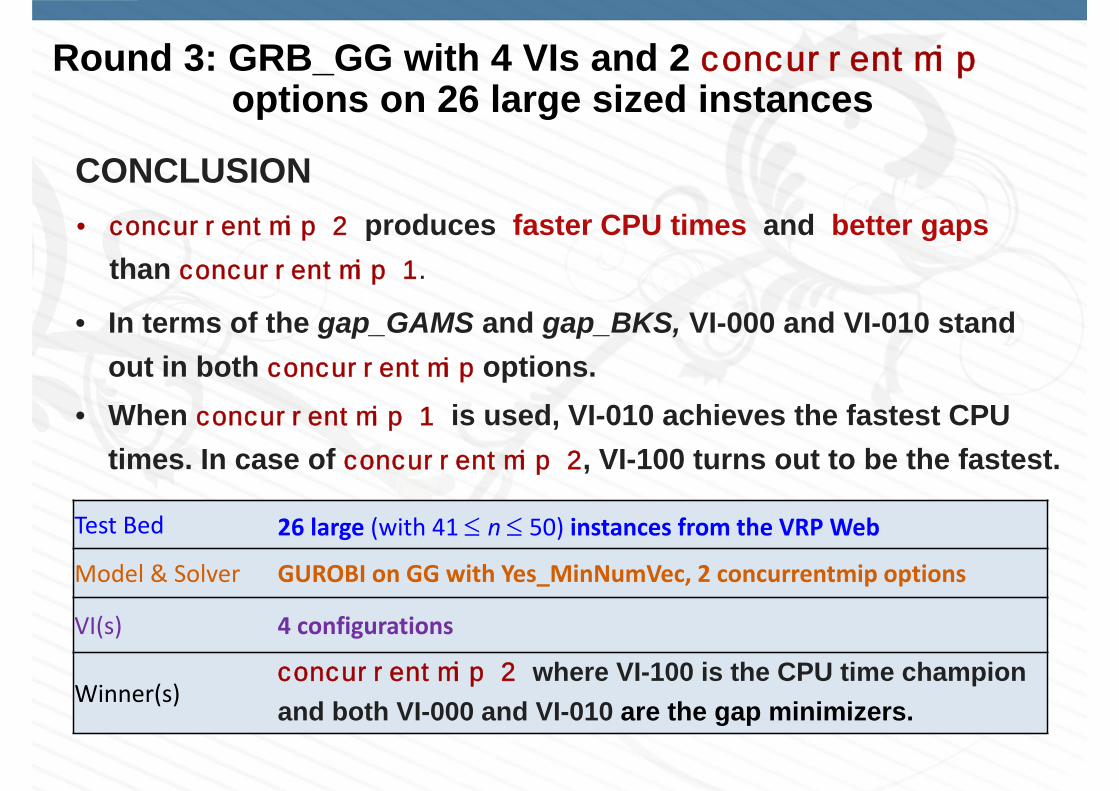
• concurrentmip 2 produces faster CPU times and better gaps than concurrentmip 1.
• In terms of the gap_GAMS and gap_BKS, VI-000 and VI-010 stand out in both concurrentmip options.
• When concurrentmip 1 is used, VI-010 achieves the fastest CPU times. In case of concurrentmip 2, VI-100 turns out to be the fastest.
Test Bed 26 large (with 41 n 50) instances from the VRP Web
Model & Solver GUROBI on GG with Yes_MinNumVec, 2 concurrentmip options
VI(s) 4 configurations
Winner(s)concurrentmip 2 where VI-100 is the CPU time champion and both VI-000 and VI-010 are the gap minimizers.
CONCLUSION

Round 4: GRB_GG on 8 asymmetric VRPLib instances with 4 VIs
Prob. Name n (No. Cust) K (No. Vehicles) BKS (Z_best)
A034‐02f 33 2 1406A036‐03f 35 3 1644A039‐03f 38 3 1654A045‐03f 44 3 1740A048‐03f 47 3 1891A056‐03f 55 3 1739A065‐03f 64 3 1974A071‐03f 70 3 2054
Note the relatively small K value (no. vehicles varying between 2 and 3)!

concurrentmip 1Average of CPU (s) Average of gap_UB_BKS Average of gap_UB_LB (GAMS)
Prob. Name 000 010 100 110 000 010 100 110 000 010 100 110
A034‐02f 2.50 2.79 5.34 3.49 0.00% 0.00% 0.00% 0.00% 0.00% 0.00% 0.00% 0.00%
A036‐03f 2.34 8.11 5.33 5.93 0.00% 0.00% 0.00% 0.00% 0.00% 0.00% 0.00% 0.00%
A039‐03f 2.27 1.25 2.16 1.25 0.00% 0.00% 0.00% 0.00% 0.00% 0.00% 0.00% 0.00%
A045‐03f 6.02 6.37 2.00 2.34 0.00% 0.00% 0.00% 0.00% 0.00% 0.00% 0.00% 0.00%
A048‐03f 4.35 4.06 3.91 4.54 0.00% 0.00% 0.00% 0.00% 0.00% 0.00% 0.00% 0.00%
A056‐03f 13.60 12.84 16.75 6.62 0.00% 0.00% 0.00% 0.00% 0.00% 0.00% 0.00% 0.00%
A065‐03f 21.84 8.25 17.20 19.13 0.00% 0.00% 0.00% 0.00% 0.00% 0.00% 0.00% 0.00%
A071‐03f 8.61 9.46 9.24 7.67 0.00% 0.00% 0.00% 0.00% 0.00% 0.00% 0.00% 0.00%Grand Average 7.69 6.64 7.74 6.37 0.00% 0.00% 0.00% 0.00% 0.00% 0.00% 0.00% 0.00%
Round 4: GRB_GG on 8 asymmetric VRPLib instances with 4 VIs

concurrentmip 2Average of CPU (s) Average of gap_UB_BKS Average of gap_UB_LB (GAMS)
Prob. Name 000 010 100 110 000 010 100 110 000 010 100 110
A034‐02f 2.82 2.14 2.72 3.67 0.00% 0.00% 0.00% 0.00% 0.00% 0.00% 0.00% 0.00%
A036‐03f 3.84 3.97 5.70 7.98 0.00% 0.00% 0.00% 0.00% 0.00% 0.00% 0.00% 0.00%
A039‐03f 1.89 1.12 2.14 1.25 0.00% 0.00% 0.00% 0.00% 0.00% 0.00% 0.00% 0.00%
A045‐03f 6.81 3.01 1.98 2.17 0.00% 0.00% 0.00% 0.00% 0.00% 0.00% 0.00% 0.00%
A048‐03f 4.19 3.17 3.68 5.98 0.00% 0.00% 0.00% 0.00% 0.00% 0.00% 0.00% 0.00%
A056‐03f 15.77 5.74 11.44 5.56 0.00% 0.00% 0.00% 0.00% 0.00% 0.00% 0.00% 0.00%
A065‐03f 22.83 6.12 17.46 7.57 0.00% 0.00% 0.00% 0.00% 0.00% 0.00% 0.00% 0.00%
A071‐03f 8.45 7.26 8.62 7.19 0.00% 0.00% 0.00% 0.00% 0.00% 0.00% 0.00% 0.00%Grand Average 8.32 4.06 6.72 5.17 0.00% 0.00% 0.00% 0.00% 0.00% 0.00% 0.00% 0.00%
Round 4: GRB_GG on 8 asymmetric VRPLib instances with 4 VIs

• Due to very few vehicles in the asymmetric VRP instances, GRB_GG with MinNumVec produces optimal solutions within seconds
regardless of the VI configuration and concurrentmip option.
• Best average CPU time is attained by VI-110 as 6.37 seconds when concurrentmip 1 is used. In case of concurrentmip 2, VI-010reduces this time to 4.06 seconds.
Test Bed 8 asymmetric instances from the VRPLib (with 33 n 70)
Model & Solver GUROBI on GG with Yes_MinNumVec, 2 concurrentmip options
VI(s) 4 configurations
Winner(s) concurrentmip 2 with VI-010
CONCLUSION
Round 4: GRB_GG on 8 asymmetric VRPLib instances with 4 VIs
Round 5: 2Com-Flow on 16 small & medium instanceswhich required at least 1 min with GRB_GG
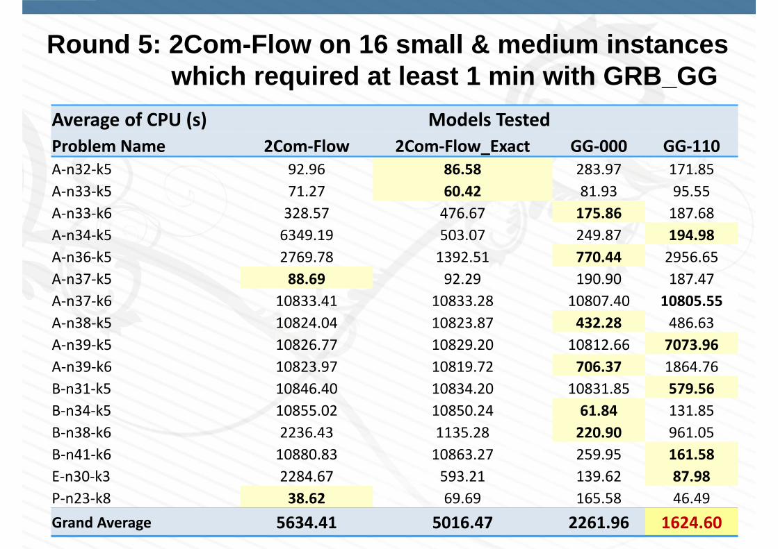
Average of CPU (s) Models TestedProblem Name 2Com‐Flow 2Com‐Flow_Exact GG‐000 GG‐110A‐n32‐k5 92.96 86.58 283.97 171.85A‐n33‐k5 71.27 60.42 81.93 95.55A‐n33‐k6 328.57 476.67 175.86 187.68A‐n34‐k5 6349.19 503.07 249.87 194.98A‐n36‐k5 2769.78 1392.51 770.44 2956.65A‐n37‐k5 88.69 92.29 190.90 187.47A‐n37‐k6 10833.41 10833.28 10807.40 10805.55A‐n38‐k5 10824.04 10823.87 432.28 486.63A‐n39‐k5 10826.77 10829.20 10812.66 7073.96A‐n39‐k6 10823.97 10819.72 706.37 1864.76B‐n31‐k5 10846.40 10834.20 10831.85 579.56B‐n34‐k5 10855.02 10850.24 61.84 131.85B‐n38‐k6 2236.43 1135.28 220.90 961.05B‐n41‐k6 10880.83 10863.27 259.95 161.58E‐n30‐k3 2284.67 593.21 139.62 87.98P‐n23‐k8 38.62 69.69 165.58 46.49Grand Average 5634.41 5016.47 2261.96 1624.60
Round 5: 2Com-Flow on 16 small & medium instanceswhich required at least 1 min with GRB_GG
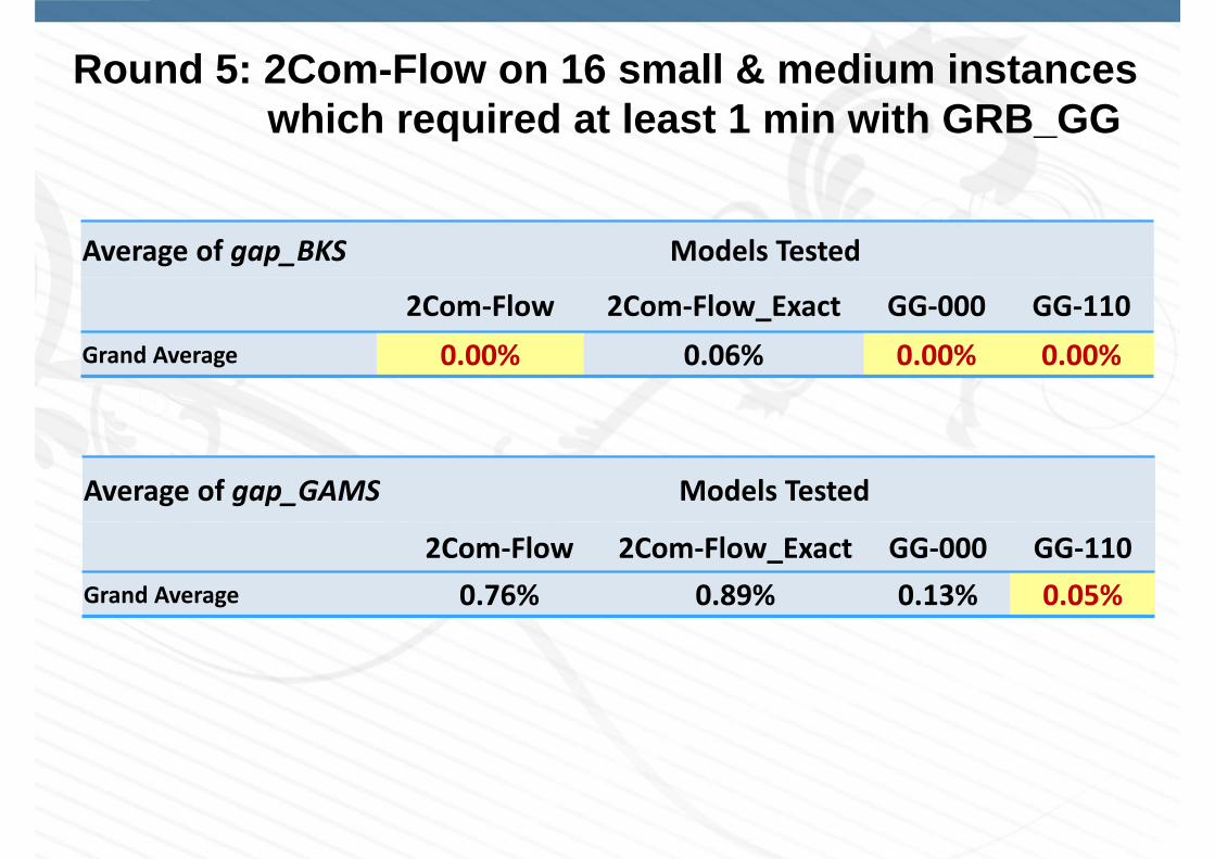
Average of gap_BKS Models Tested
2Com‐Flow 2Com‐Flow_Exact GG‐000 GG‐110Grand Average 0.00% 0.06% 0.00% 0.00%
Average of gap_GAMS Models Tested
2Com‐Flow 2Com‐Flow_Exact GG‐000 GG‐110Grand Average 0.76% 0.89% 0.13% 0.05%
Round 5: 2Com-Flow on 16 small & medium instanceswhich required at least 1 min with GRB_GG
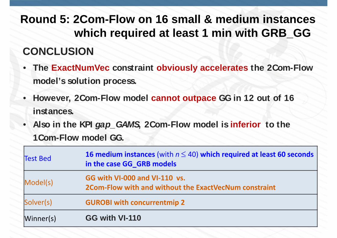
• The ExactNumVec constraint obviously accelerates the 2Com-Flow model’s solution process.
Test Bed 16 medium instances (with n 40) which required at least 60 seconds in the case GG_GRB models
Model(s) GG with VI‐000 and VI‐110 vs. 2Com‐Flow with and without the ExactVecNum constraint
Solver(s) GUROBI with concurrentmip 2
Winner(s) GG with VI-110
CONCLUSION
• However, 2Com-Flow model cannot outpace GG in 12 out of 16 instances.
• Also in the KPI gap_GAMS, 2Com-Flow model is inferior to the 1Com-Flow model GG.
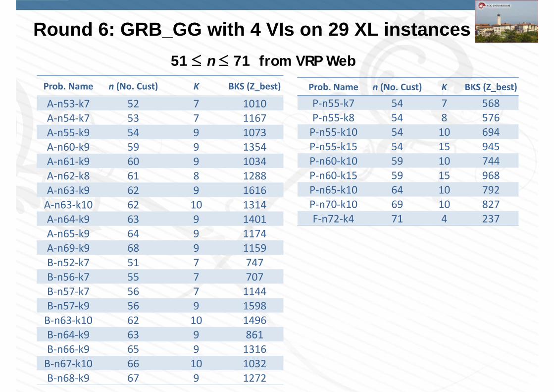
Round 6: GRB_GG with 4 VIs on 29 XL instances
Prob. Name n (No. Cust) K BKS (Z_best)
A‐n53‐k7 52 7 1010A‐n54‐k7 53 7 1167A‐n55‐k9 54 9 1073A‐n60‐k9 59 9 1354A‐n61‐k9 60 9 1034A‐n62‐k8 61 8 1288A‐n63‐k9 62 9 1616A‐n63‐k10 62 10 1314A‐n64‐k9 63 9 1401A‐n65‐k9 64 9 1174A‐n69‐k9 68 9 1159B‐n52‐k7 51 7 747B‐n56‐k7 55 7 707B‐n57‐k7 56 7 1144B‐n57‐k9 56 9 1598B‐n63‐k10 62 10 1496B‐n64‐k9 63 9 861B‐n66‐k9 65 9 1316B‐n67‐k10 66 10 1032B‐n68‐k9 67 9 1272
Prob. Name n (No. Cust) K BKS (Z_best)
P‐n55‐k7 54 7 568P‐n55‐k8 54 8 576P‐n55‐k10 54 10 694P‐n55‐k15 54 15 945P‐n60‐k10 59 10 744P‐n60‐k15 59 15 968P‐n65‐k10 64 10 792P‐n70‐k10 69 10 827F‐n72‐k4 71 4 237
51 n 71 from VRP Web
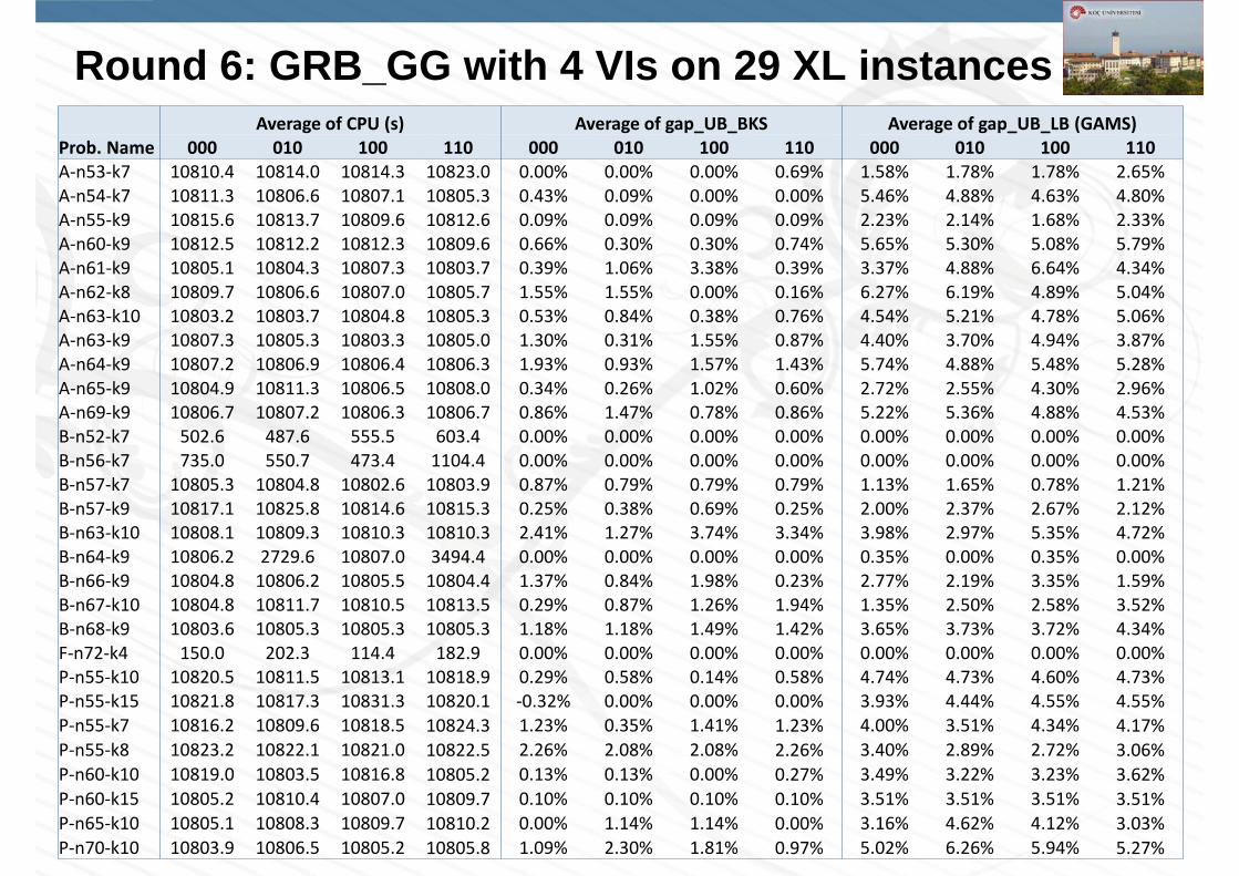
Round 6: GRB_GG with 4 VIs on 29 XL instancesAverage of CPU (s) Average of gap_UB_BKS Average of gap_UB_LB (GAMS)
Prob. Name 000 010 100 110 000 010 100 110 000 010 100 110A‐n53‐k7 10810.4 10814.0 10814.3 10823.0 0.00% 0.00% 0.00% 0.69% 1.58% 1.78% 1.78% 2.65%A‐n54‐k7 10811.3 10806.6 10807.1 10805.3 0.43% 0.09% 0.00% 0.00% 5.46% 4.88% 4.63% 4.80%A‐n55‐k9 10815.6 10813.7 10809.6 10812.6 0.09% 0.09% 0.09% 0.09% 2.23% 2.14% 1.68% 2.33%A‐n60‐k9 10812.5 10812.2 10812.3 10809.6 0.66% 0.30% 0.30% 0.74% 5.65% 5.30% 5.08% 5.79%A‐n61‐k9 10805.1 10804.3 10807.3 10803.7 0.39% 1.06% 3.38% 0.39% 3.37% 4.88% 6.64% 4.34%A‐n62‐k8 10809.7 10806.6 10807.0 10805.7 1.55% 1.55% 0.00% 0.16% 6.27% 6.19% 4.89% 5.04%A‐n63‐k10 10803.2 10803.7 10804.8 10805.3 0.53% 0.84% 0.38% 0.76% 4.54% 5.21% 4.78% 5.06%A‐n63‐k9 10807.3 10805.3 10803.3 10805.0 1.30% 0.31% 1.55% 0.87% 4.40% 3.70% 4.94% 3.87%A‐n64‐k9 10807.2 10806.9 10806.4 10806.3 1.93% 0.93% 1.57% 1.43% 5.74% 4.88% 5.48% 5.28%A‐n65‐k9 10804.9 10811.3 10806.5 10808.0 0.34% 0.26% 1.02% 0.60% 2.72% 2.55% 4.30% 2.96%A‐n69‐k9 10806.7 10807.2 10806.3 10806.7 0.86% 1.47% 0.78% 0.86% 5.22% 5.36% 4.88% 4.53%B‐n52‐k7 502.6 487.6 555.5 603.4 0.00% 0.00% 0.00% 0.00% 0.00% 0.00% 0.00% 0.00%B‐n56‐k7 735.0 550.7 473.4 1104.4 0.00% 0.00% 0.00% 0.00% 0.00% 0.00% 0.00% 0.00%B‐n57‐k7 10805.3 10804.8 10802.6 10803.9 0.87% 0.79% 0.79% 0.79% 1.13% 1.65% 0.78% 1.21%B‐n57‐k9 10817.1 10825.8 10814.6 10815.3 0.25% 0.38% 0.69% 0.25% 2.00% 2.37% 2.67% 2.12%B‐n63‐k10 10808.1 10809.3 10810.3 10810.3 2.41% 1.27% 3.74% 3.34% 3.98% 2.97% 5.35% 4.72%B‐n64‐k9 10806.2 2729.6 10807.0 3494.4 0.00% 0.00% 0.00% 0.00% 0.35% 0.00% 0.35% 0.00%B‐n66‐k9 10804.8 10806.2 10805.5 10804.4 1.37% 0.84% 1.98% 0.23% 2.77% 2.19% 3.35% 1.59%B‐n67‐k10 10804.8 10811.7 10810.5 10813.5 0.29% 0.87% 1.26% 1.94% 1.35% 2.50% 2.58% 3.52%B‐n68‐k9 10803.6 10805.3 10805.3 10805.3 1.18% 1.18% 1.49% 1.42% 3.65% 3.73% 3.72% 4.34%F‐n72‐k4 150.0 202.3 114.4 182.9 0.00% 0.00% 0.00% 0.00% 0.00% 0.00% 0.00% 0.00%P‐n55‐k10 10820.5 10811.5 10813.1 10818.9 0.29% 0.58% 0.14% 0.58% 4.74% 4.73% 4.60% 4.73%P‐n55‐k15 10821.8 10817.3 10831.3 10820.1 ‐0.32% 0.00% 0.00% 0.00% 3.93% 4.44% 4.55% 4.55%P‐n55‐k7 10816.2 10809.6 10818.5 10824.3 1.23% 0.35% 1.41% 1.23% 4.00% 3.51% 4.34% 4.17%P‐n55‐k8 10823.2 10822.1 10821.0 10822.5 2.26% 2.08% 2.08% 2.26% 3.40% 2.89% 2.72% 3.06%P‐n60‐k10 10819.0 10803.5 10816.8 10805.2 0.13% 0.13% 0.00% 0.27% 3.49% 3.22% 3.23% 3.62%P‐n60‐k15 10805.2 10810.4 10807.0 10809.7 0.10% 0.10% 0.10% 0.10% 3.51% 3.51% 3.51% 3.51%P‐n65‐k10 10805.1 10808.3 10809.7 10810.2 0.00% 1.14% 1.14% 0.00% 3.16% 4.62% 4.12% 3.03%P‐n70‐k10 10803.9 10806.5 10805.2 10805.8 1.09% 2.30% 1.81% 0.97% 5.02% 6.26% 5.94% 5.27%
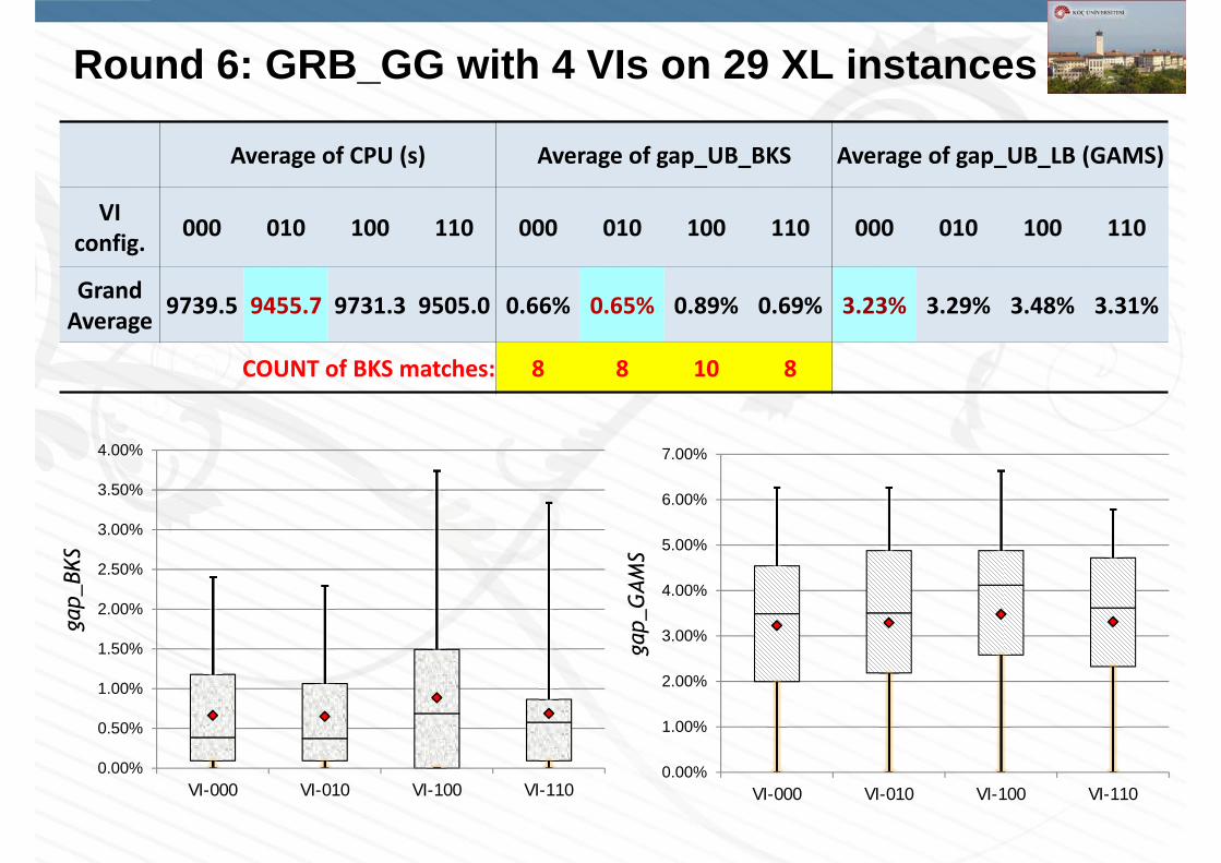
Round 6: GRB_GG with 4 VIs on 29 XL instances
Average of CPU (s) Average of gap_UB_BKS Average of gap_UB_LB (GAMS)
VI config. 000 010 100 110 000 010 100 110 000 010 100 110
Grand Average 9739.5 9455.7 9731.3 9505.0 0.66% 0.65% 0.89% 0.69% 3.23% 3.29% 3.48% 3.31%
COUNT of BKS matches: 8 8 10 8
0.00%
0.50%
1.00%
1.50%
2.00%
2.50%
3.00%
3.50%
4.00%
VI-000 VI-010 VI-100 VI-110
gap_
BKS
0.00%
1.00%
2.00%
3.00%
4.00%
5.00%
6.00%
7.00%
VI-000 VI-010 VI-100 VI-110
gap_
GA
MS
Round 6: GRB_GG with 4 VIs on 29 XL instances
• GRB_GG with MinNumVec and no other VIs can yield an average gap_GAMS of 3.23% at the end of 3 hours.
Test Bed 29 XL size instances (with 51 n 71) from VRP Web
Model(s) GG with MinNumVec constraint and four VI configurations.
Solver(s) GUROBI with concurrentmip 2
Winner(s) GG with VI-010
CONCLUSION
• GRB_GG with MinNumVec and VI-010 achieves an average gap_BKSof 0.65% at the end of 3 hours. When the 2nd VI is omitted (i.e., with VI-000), this KPI value rises to 0.66%.
• Not only is GRB_GG with MinNumVec and VI-010 a tiny bit better in BFS quality, but also slightly faster than the other three VIs.
Round 7: GRB_GG with 4 Granular VIs on 29 XL instances
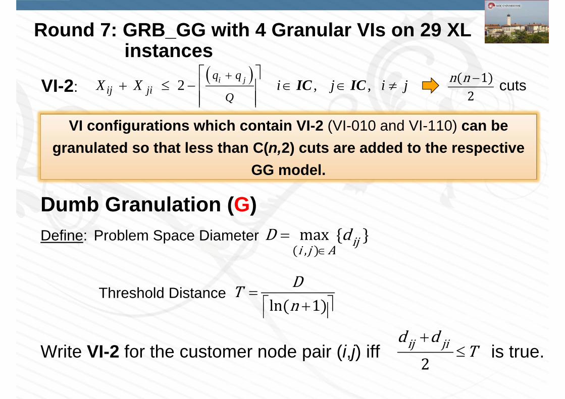
VI-2:
2 , ,
i jij ji
q q
QX X i j i j IC IC cuts1
2n n
Dumb Granulation (G)Define: Problem Space Diameter
Threshold Distance
Write VI-2 for the customer node pair (i,j) iff is true.
,max iji j A
D d
ln 1DTn
2ij jid d
T
VI configurations which contain VI-2 (VI-010 and VI-110) can be granulated so that less than C(n,2) cuts are added to the respective
GG model.

Round 7: GRB_GG with 4 Granular VIs on 29 XL instances
VI-2:
Smart Granulation through Clustering (GC)Design: K clusters using a greedy clustering algorithm in O(n2) time.
Extract: The distance values dij for each customer node pair (i,j IC) that is intracluster (both i and j are located within the same cluster).
Sort: All intracluster distance values dij in ascending order.
Write VI-2 only for the (i,j) pairs corresponding to the FIRST (smallest) K(n+1) dij values.
2 , ,
i j
ij jiq q
QX X i j i j IC IC cuts1
2n n
Round 7: GRB_GG with 4 Granular VIs on 29 XL instances
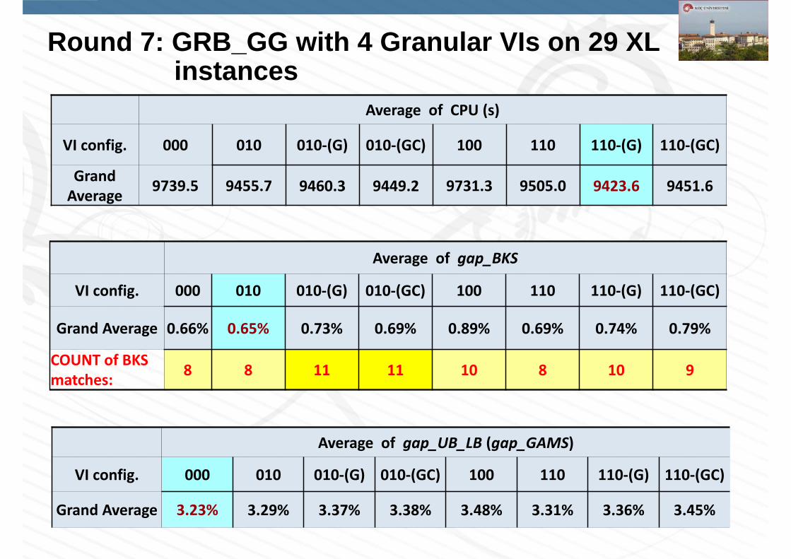
Average of CPU (s)
VI config. 000 010 010‐(G) 010‐(GC) 100 110 110‐(G) 110‐(GC)
Grand Average 9739.5 9455.7 9460.3 9449.2 9731.3 9505.0 9423.6 9451.6
Average of gap_UB_LB (gap_GAMS)
VI config. 000 010 010‐(G) 010‐(GC) 100 110 110‐(G) 110‐(GC)
Grand Average 3.23% 3.29% 3.37% 3.38% 3.48% 3.31% 3.36% 3.45%
Average of gap_BKS
VI config. 000 010 010‐(G) 010‐(GC) 100 110 110‐(G) 110‐(GC)
Grand Average 0.66% 0.65% 0.73% 0.69% 0.89% 0.69% 0.74% 0.79%
COUNT of BKS matches: 8 8 11 11 10 8 10 9
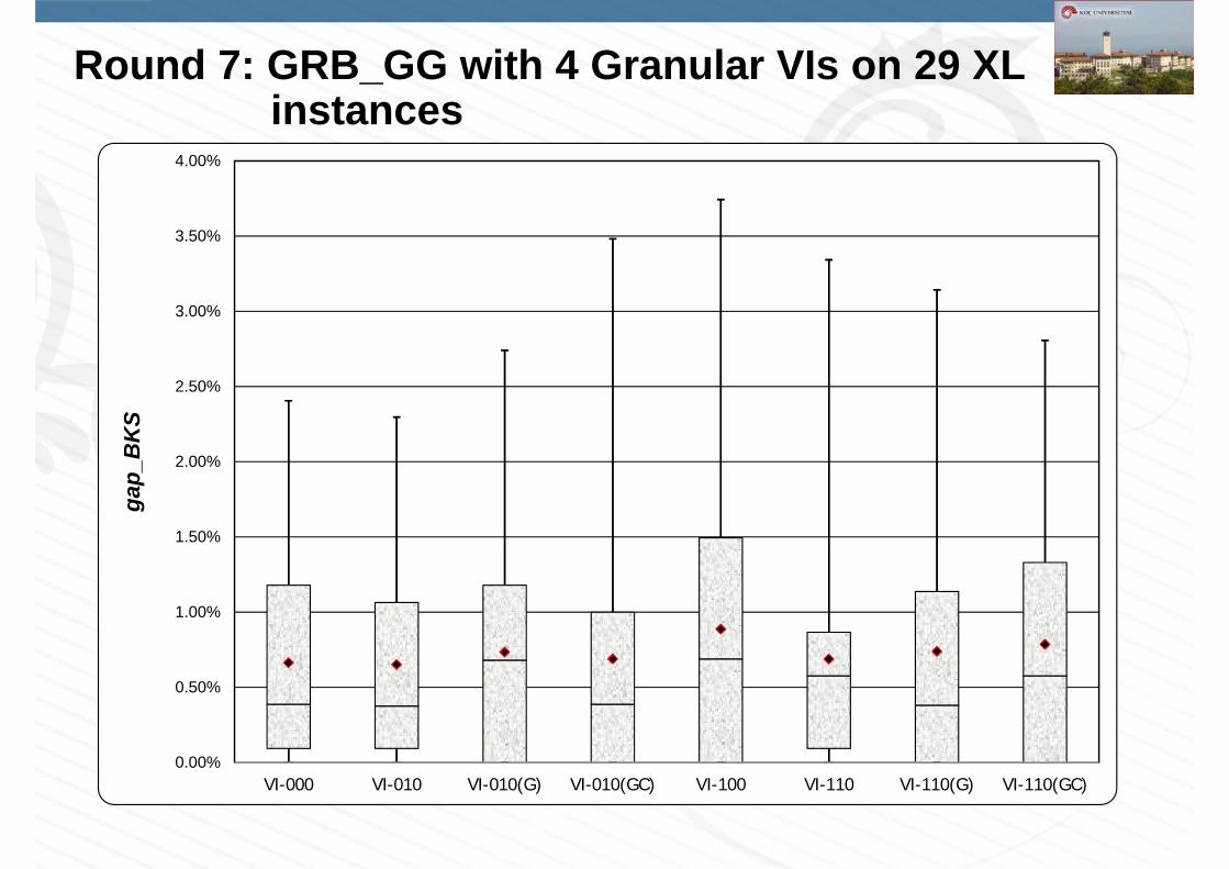
Round 7: GRB_GG with 4 Granular VIs on 29 XL instances
0.00%
0.50%
1.00%
1.50%
2.00%
2.50%
3.00%
3.50%
4.00%
VI-000 VI-010 VI-010(G) VI-010(GC) VI-100 VI-110 VI-110(G) VI-110(GC)
gap_
BK
S
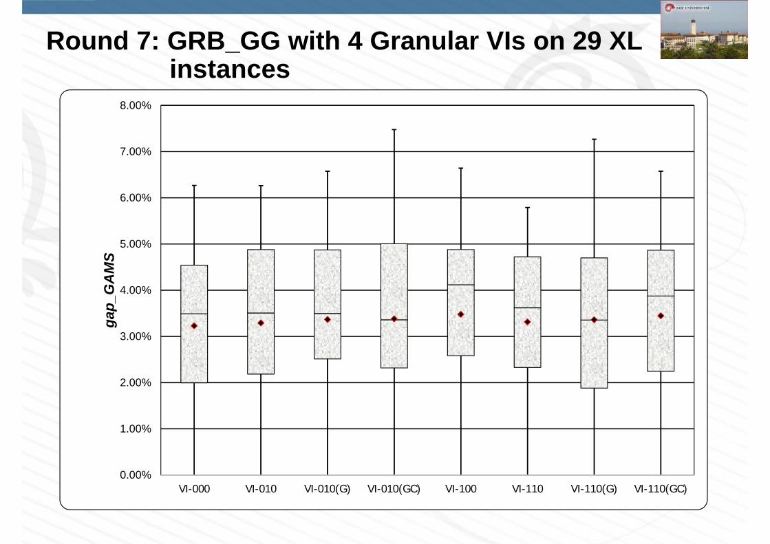
Round 7: GRB_GG with 4 Granular VIs on 29 XL instances
0.00%
1.00%
2.00%
3.00%
4.00%
5.00%
6.00%
7.00%
8.00%
VI-000 VI-010 VI-010(G) VI-010(GC) VI-100 VI-110 VI-110(G) VI-110(GC)
gap_
GA
MS
OVERVIEW Introduction and motivation Lifted_MTZ, 1Com-Flow (GG) and 2Com-Flow formulations Experimental setup and results
– Round 1: Gurobi (GRB) and Cplex (CPL) on GG and Lifted_MTZ models of 39 small and medium sized instances
• Effect of the MinNumVec constraint as a valid inequality (VI)
– Round 2: GRB on GG with all VIs and concurrentmip options
– Round 3: GRB_GG with 4 VIs and 2 concurrentmip options on 26 large sized instances
– Round 4: GRB_GG on 8 asymmetric VRPLib instances with 4 VIs
– Round 5: 2Com-Flow formulation on 16 medium sized instances
• Effect of the ExactNumVec constraint as a VI
– Round 6: GRB_GG on 29 XL sized instances with 2 VIs
– Round 7: GRB_GG on 29 XL sized instances with 4 Granular VI Configurations
Conclusion
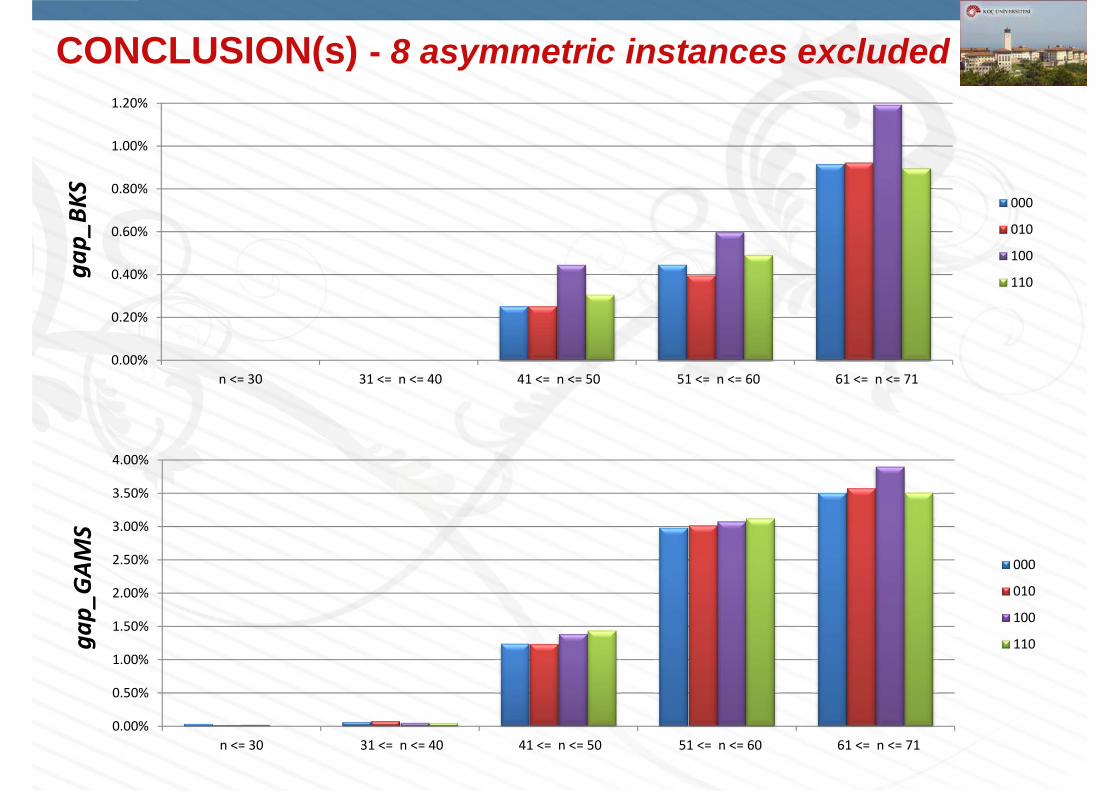
CONCLUSION(s) - 8 asymmetric instances excluded
0.00%
0.20%
0.40%
0.60%
0.80%
1.00%
1.20%
n <= 30 31 <= n <= 40 41 <= n <= 50 51 <= n <= 60 61 <= n <= 71
gap_
BKS
000
010
100
110
0.00%
0.50%
1.00%
1.50%
2.00%
2.50%
3.00%
3.50%
4.00%
n <= 30 31 <= n <= 40 41 <= n <= 50 51 <= n <= 60 61 <= n <= 71
gap_
GAM
S
000
010
100
110
CONCLUSION(s) - 8 asymmetric instances excluded
0
1000
2000
3000
4000
5000
6000
7000
8000
9000
10000
n <= 30 31 <= n <= 40 41 <= n <= 50 51 <= n <= 60 61 <= n <= 71
CPU times (s)
000
010
100
110
0%
10%
20%
30%
40%
50%
60%
70%
80%
90%
100%
n <= 30 31 <= n <= 40 41 <= n <= 50 51 <= n <= 60 61 <= n <= 71
Ratio
of B
KS fo
und
000
010
100
110
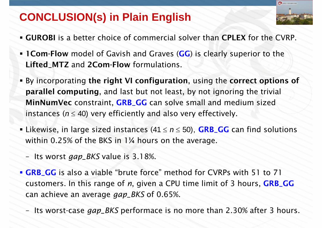
CONCLUSION(s) in Plain English
GUROBI is a better choice of commercial solver than CPLEX for the CVRP.
1Com-Flow model of Gavish and Graves (GG) is clearly superior to the Lifted_MTZ and 2Com-Flow formulations.
By incorporating the right VI configuration, using the correct options of
parallel computing, and last but not least, by not ignoring the trivial MinNumVec constraint, GRB_GG can solve small and medium sized instances (n 40) very efficiently and also very effectively.
Likewise, in large sized instances (41 n 50), GRB_GG can find solutions within 0.25% of the BKS in 1¼ hours on the average.
– Its worst gap_BKS value is 3.18%.
GRB_GG is also a viable “brute force” method for CVRPs with 51 to 71 customers. In this range of n, given a CPU time limit of 3 hours, GRB_GG
can achieve an average gap_BKS of 0.65%.
– Its worst-case gap_BKS performace is no more than 2.30% after 3 hours.

Questions?