oec 1 4 1972 transverse diffusion of solutes in natural ... · transverse diffusion of solutes in...

Transverse Diffusion of

Solutes in Natural Streams

OEC 1 4 1972

GEOLOGICAL SURVEY PROFESSIONAL PAPER 582-C

Transverse Diffusion of

Solutes in Natural Streams By NOBUHIRO YOTSUKURA and ERNEST D. COBB

DISPERSION IN SURFACE WATER

GEOLOGICAL SURVEY PROFESSIONAL PAPER 582-C

UNITED STATES GOVERNMENT PRINTING OFFICE. WASHINGTON : 1972

UNITED STATES DEPARTMENT OF THE INTERIOR

ROGERS C. B. MORTON, Secretary

GEOLOGICAL SURVEY

V. E. McKelvey, Director

Library of Congress catalog-card No. 72-600198

For sale by the Superintendent of Documents, U.S. Government Printing Office Washington, D.C. 20402- Price 55 cents (paper cover)

Stock Number 2401-2147

CONTENTS

Page

Abstract___________________________________________________________________ C1 Introduction_______________________________________________________________ 1 Acknowledgments____________________________________________________________ 2 Equation of transverse diffusion______________________________________________ 2 Analytical solutions_________________________________________________________ 4 Procedure for verification by stream data______________________________________ 6 South River test____________________________________________________________ 6 Atrisco Feeder Canal test____________________________________________________ 9 Bernardo Conveyance Channel test___________________________________________ 12 Missouri River test_________________________________________________________ 13 Applications_______________________________________________________________ 15 Conclusions________________________________________________________________ 19 References_________________________________________________________________ 19

ILLUSTRATIONS

Page

FIGURE 1. Sketch of an infinitesimal stream tube in a natural stream_______________________________________________ C2 2. Effects of variable diffusion factor on the solutions to diffusion equation _______________________ ------------ 4

3-5. Comparison of observed and theoretical concentration distribution: 3. South River test L ___ _ __ _ _ _ _ _ _ _ _ _ __ __ _ __ ___ _ ____ __ __ __ _ _ ___ __ __ ____ __ __ __ __ __ ___ _ _ ____ __ __ __ 7

4. South River test 2--------------------------------------------------------------------------- 8 5. South River test 3_ ___ _ _ _ _ _ _ _ _ _ _ __ __ __ __ __ _ _ __ _ _ __ _ __ _ __ ___ _ _ _ _ _ _ __ _ _ ___ ____ __ __ _ ___ ____ ___ _ _ 8

6. Comparison of concentration-transverse distance curve and concentration-cumulative discharge curve, South River test 2----------------------------------------------------------------------------------- 9

7-10. Comparison of observed and theoretical concentration distribution: 7. Atrisco Feeder Canal test L _ _ __ _ _ _ __ __ __ _ _ __ __ __ __ __ __ _ _ _ _ __ _ __ _ _ _ _ _ _ _ _ __________ _ _ _ __ _ _ _ __ _ _ 10

8. Atrisco Feeder Canal test 2------------------------------------------------------------------- 11 9. Atrisco Feeder Canal test 3 _ _ _ _ _ _ _ _ _ _ _ _ _ _ _ _ _ _ _ _ _ _ _ _ _ _ _ _ _ _ _ _ _ _ _ _ _ _ _ _ _ _ _ _ _ _ _ _ _ _ _ _ _ _ _ _ _ _ _ _ _ _ _ _ _ _ _ 11

10. Bernardo Conveyance Channel________________________________________________________________ 13 11. Relation of relative cumulative discharge to relative transverse distance, Missouri River near Blair, Nebr _ _ _ _ _ 14 12. Comparison of observed and theoretical concentration distribution, Missouri River near Blair, Nebr__________ 14

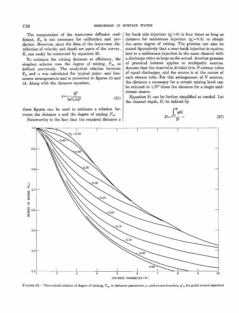
13-14. Theoretical relation of degree of mixing, Pm: 13. To distance parameter, a, and source location q/, for point source injections_______________________ 16 14. To distance parameter, a, and source location, qat' and q82 ', for line source injections________________ 17

TABLES

TABLE 1-4. Computation of best-fit transverse diffusion coefficients: Page 1. South River_________________________________________________________________________________ C9 2. Atrisco Feeder Canal_________________________________________________________________________ 12 3. Bernardo Conveyance Channel________________________________________________________________ 12 4. Missouri River near Blair, N ebr_ _______________________________________________________ ------- 15

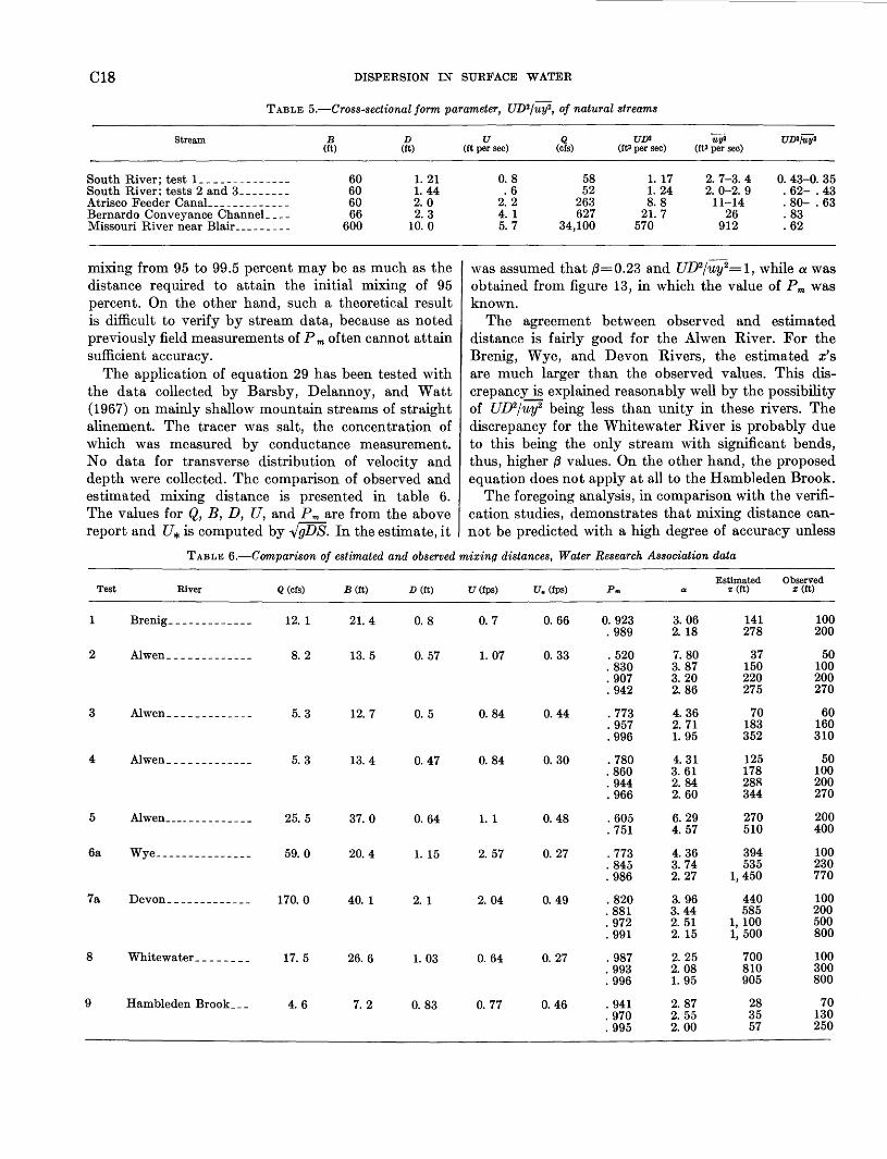
5. Cross-sectional form parameter, UD2juy2, of natural streams___________________________________________ 18 6. Comparison of estimated and observed mixing distances, Water Research Association data ____ ------------- 18

III

DISPERSION IN SURFACE WATER

TRANSVERSE DIFFUSION OF SOLUTES IN NATURAL STREAMS

By N OBUHIRO YoTSUKURA and ERNEST D. CoBB

ABSTRACT

An analytical model is developed for the transverse diffusion of solutes from steady sources placed in a natural stream with steady discharge.

In theoretical derivations, the steady-state convective diffusion equation for a natural stream is convertEd into an approximate equation suitable for analytical treatment by the introduction of cumulative partial discharge as an independent variable. Analytical solutions for the latter equation are obtained for point and line source injections of solutes.

The validity of the model is tested using data from four natural streams, three of which are alined straight, while one has mild curves. The verification was satisfactory for the three straight channels, and the constant in Elder's formula for the transverse diffusion coefficient ranged from 0.2 to 0.3. In the curved channel, the model appears workable, but an increase of the diffusion coefficient in the downstream direction is observed.

The applications to stream problems are discussed in the final section. The model may be employed for the description and prediction of thermal and other waste disposal problems, simulation studies by tracers, and the determination of transverse diffusion coefficient. Another use of the model, the estimation of mixing distances, is explained and demonstrated using the data of the Water Research Association, England.

INTRODUCTION

The transverse diffusion (mixing) of soluble material in natural streams is an important mechanism of transport in the disposal and dispersal of industrial and municipal wastes in streams. Thanks to the frequent reporting of mass media, the public is now familiar with infrared photography of polluted streams in which a plume of hot waste water is often shown hugging a bank for miles downstream without substantial mixing with the rest of the flow. A careful observer traveling by airplane will sometimes notice the same phenomenon dowstream from the junction of a clear main stream and a sediment-laden tributary. Observations on the behavior of pollutants and tracers have established that, while v-ertical mixing is completed in a relatively short downstream distance, a much longer distance is

required for the completion of transverse mixing in natural water courses.

Despite most waste releases being in the form of a point source, which induces highly nonuniform distribution of waste concentration in a cross section, the design of an outfall and the evaluation of downstream pollution have often been !>ased on the vague concept that the waste is somehow dispersed uniformly throughout an arbitrary volume of receiving water. There appears to be no standard to evaluate the merit of point release against line release or that of bank-side release against midstream release. Many ordinances for thermal loading of streams refer to the so-called mixing zone without any quantitative definition of the zone. Again there is no accepted method of estimating the distance and degree of mixing under various loading conditions.

There obviously is a need to establish a workable model of transverse diffusion in natural streams to provide answers to the above problems, as well as other questions pertaining to efficient pollution control. Knowledge of the transverse diffusion coefficient is a prerequisite in assessing the total dispersive capacity of a stream. As the recent study of Fischer (1967a) has shown, longitudinal dispersion in open channel flow is due to the combined action of variable longitudinal convection along the transverse axis and turbulent diffusion in the transverse direction. Whether the longitudinal dispersion is described in terms of the effective dispersion coefficient or by means of numerical simulation, knowing the transverse diffusion coefficient is vital.

A review of the literature on transverse diffusion is helpful to delineate further the objectives of the present study. A basic source of information on transverse diffusion is Elder (1959), who found from his flume experiment that the transverse distribution of solute in two-dimensional flow is Gaussian and that the

Cl

C2 DISPERSION IN SURFACE WATER

transverse diffusion coefficient, Ez, is given by

(1)

where D is the depth of flow and U * is the average shear velocity. The constant, {3, was given by Elder as 0.23. Orlob (1959), Sayre and Chamberlain (1964), Sayre and Chang (1968), Engelund (1969), and Prych (1970) investigated the diffusion of plastic particles floating on the surface of a two-dimensional flume flow and obtained the value of {3 ranging from 0.17 to 0.26. According to Prych's (1970) summary of the depthaveraged transverse diffusion coefficient, the values of {3 in a laboratory flume range from 0.11 (Sullivan, 1968), to 0.18 (Sayre and Chang, 1968). Prych also shows that the correct value of {3 for Elder's data is 0.16 rather than 0.23 and is in good agreement with his and Okoye's measured value of 0.14. Fischer (1967a) confirmed that the transverse solute distribution in a three-dimensional flume flow can be predicted satisfactorily by the use of {3=0.23. Sayre and Chang (1968) concluded that the Fickian diffusion theory including the reflectionsuperposition technique is satisfactory in describing the transverse diffusion of solute in a rectangular flume. Recently Fischer (1969) proposed a method of estimating the transverse diffusion coefficient in stream bends and showed that t.he secondary currents could increase the constant of equation 1 as much as tenfold.

In comparison with laboratory flume studies, information on diffusion in natural streams is rather limited. Glover (1964) obtained {3=0.72 in a reach of the Columbia River by using a mixture of radioisotopes as a tracer. He then used the reflection-superposition principle to predict the diffusion at a large distance from the source and obtained fair agreement with observed data. Fischer (1967b) reported a {3 value of 0.24 measured in a straight reach of the Atrisco Feeder Canal, an irrigation canal 2 feet deep and 60 feet wide. Lately, Yotsukura, Fischer, and Sayre (1970) reported the value of Ez=0.6DU* as observed in the Missouri River. In contrast to the moment method used by Glover and Fischer, Yotsukura, Fischer, and Sayre used a numerical simulation of the diffusion equation to determine the transverse diffusion coefficient.

Two points about transverse diffusion are apparent from the above review. The first is that the form of the transverse diffusion coefficient is now well established by equation 1, even though the value of the constant, ~' may vary considerably between laboratory flumes and natural streams. The second is that, as long as there is no appreciable convective transport in the transverse direction, application of the Fickian theory

with much basic information compiled, it appears feasible and appropriate to integrate it into a workable model of transverse diffusion which is directly applicable to waste disposal problems.

This report presents a comprehensive study on the steady-state transverse diffusion of solute in natural streams. The theoretical part of the study derives an appropriate diffusion equation and then red~ces itt? a form suitable for analytical treatment by IntroduCing the cumulative partial discharge, q, as the independent variable replacing the transverse distance, z. The transformation provides a convenient means of accounting for the solute mass balance and of adapting the analytical solutions as adequate approximations to stream conditions with variable velocity u(z). A set of analytical solutions for a point source and a line source are obtained by the method of images. The theoretical development is then compared with diffusion data from a number of streams, and the results are presented as a table of computed transverse diffusion coefficient and as a graphic comparison of observed versus theoretical concentration distribution. Several applications of the theory are presented in the final section.

ACKNOWLEDGMENTS

The dye diffusion tests in Atrisco Feeder Canal and , Bernardo Conveyance Channel were conducted under the direction of James K. Culbertson. H. B. Fischer, D. R. Dawdy, and C. F. Nordin participated in the tests. M. A. Kennan rendered valuable assistance throughout the present study. Contributions of the above-mentioned U.S. Geological Survey personnel are gratefully acknowledged.

EQUATION OF TRANSVERSE DIFFUSION

Consider a uniform section of a steady natural stream as sketched in figure 1. The coordinate x is measured in the longitudinal (downstream) direction, y is directe.d vertically downward from the water surface, and z IS

is satisfactory for transverse diffusion problems. Now FIGURE 1.-An infinitesimal stream tube in a natural stream

TRANSVERSE DIFFUSION OF SOLUTES IN NATURAL STREAMS C3

measured transversely from the left bank along the water surface. It is assumed that the section is far enough downstream from the solute injection site that the vertical distribution of solute concentration is already uniform. The problem is thus restricted to two space dimensions and the vertical variation of such quantities as velocity, diffusion coefficients, and solute concentration is neglected through the use of depthaveraged values. Density of water is assumed to be homogeneous through the system. The symbol y is used to denote the flow depth measured from the water surface to the channel bed and is thus a function of z.

The transport (convective diffusion) equation of a solute is derived for an elementary volume yt::.zt::.x containing a solute concentration, c, by noting that the mass continuity of solute within the volume must be satisfied at any time. The net inflow rate of solute due to the convective velocity u(z) into the volume yt::.zt::.x is given by

The net inflow rate due to transverse diffusion, for which the diffusion coefficient is designated by Ez(z), is expressed by

The time rate of increase of solute mass within the volume is given by

a(cyt::.xt::.z) -at-·

The sum of inflow rates of solute through all boundaries is now equated to the time rate of change in order to satisfy the mass continuity, and the following equation of solute transport is obtained

(2)

In this derivation the convective velocity is assumed to act only in the longitudinal direction so the volume yt::.zt::.x forms a stream tube. Also the turbulent diffusion in the longitudinal direction is neglected because the transport due to this diffusion is very small relative to the transport by the convection and transverse diffusion.

The equation of steady-state transverse diftusion is a special case of equation 2 when it is assumed that the solute is injected into the stream continuously at a uniform rate. Since the solute concentration c at any

downstream location will give a value which is independent of time, the time derivative term in equation 2 is dropped. Furthermore, since u, y, and Ez are assumed to be functions of z alone, equation 2 is simplified to the form

(3)

The boundary conditions at the banks are given by

ac EzYaz =0 at z=O and B (4)

where B is the channel width. Because of the steady state of solute distribution, the inflow rate of solute at the injection site must be equal to the outflow rate at a downstream cross section or

M='Y J: cuydz, (5)

where M is the time rate of solute inflow by weight and 'Y is the specific weight of water.

When u andy vary transversely as in typical natural streams, it is impossible to obtain closed-form analytical solutions to equations 3, 4, and 5. The only feasible method of solving them directly is to use a finite-difference technique with a digital computer. In various applications, however, it is desirable to have analytical solutions which can be used for the approximation of real problems, because direct numerical simulation which normally requires time-consuming preparation of input data may not be justified in terms of time and cost.

A new independent variable q will be defined by

(6)

It is seen that q is the cumulative discharge measured from the left bank and becomes Q at z=B, where Q is the total discharge. By introducing q in place of z, equations 3, 4, and 5 are transformed to

OC 0 ( 20C) ox= oq EzUY oq (7)

oc Ezuy2

0q =0 at q=O and Q (8)

M="fiQcdq· (9)

Equation 7 may "be considered as the diffusion equation with convective velocity of unity and transverse diffusion coefficient of EzUY 2

• Even though equation 7 appears more suitable for analytical treatments than


equation 3, such analytical solutions have not been 1

obtained and the solution must still be sought through numerical techniques.

Fortunately there is strong empirical evidence that the solution to equation 7 having a variable coefficient e,uy2 (henceforth called diffusion factor to differentiate it from the diffusion coefficient e2) can be approximated sufficiently by the solution of another equation having a constant factor EzUY2

, or

de -- d2c dX =ezUY2 (jq2' (10)

where e2uy2 is the constant diffusion factor defined by

- 1.J:Q E2Uy2=Q 0

E2Uy2dq. (11)

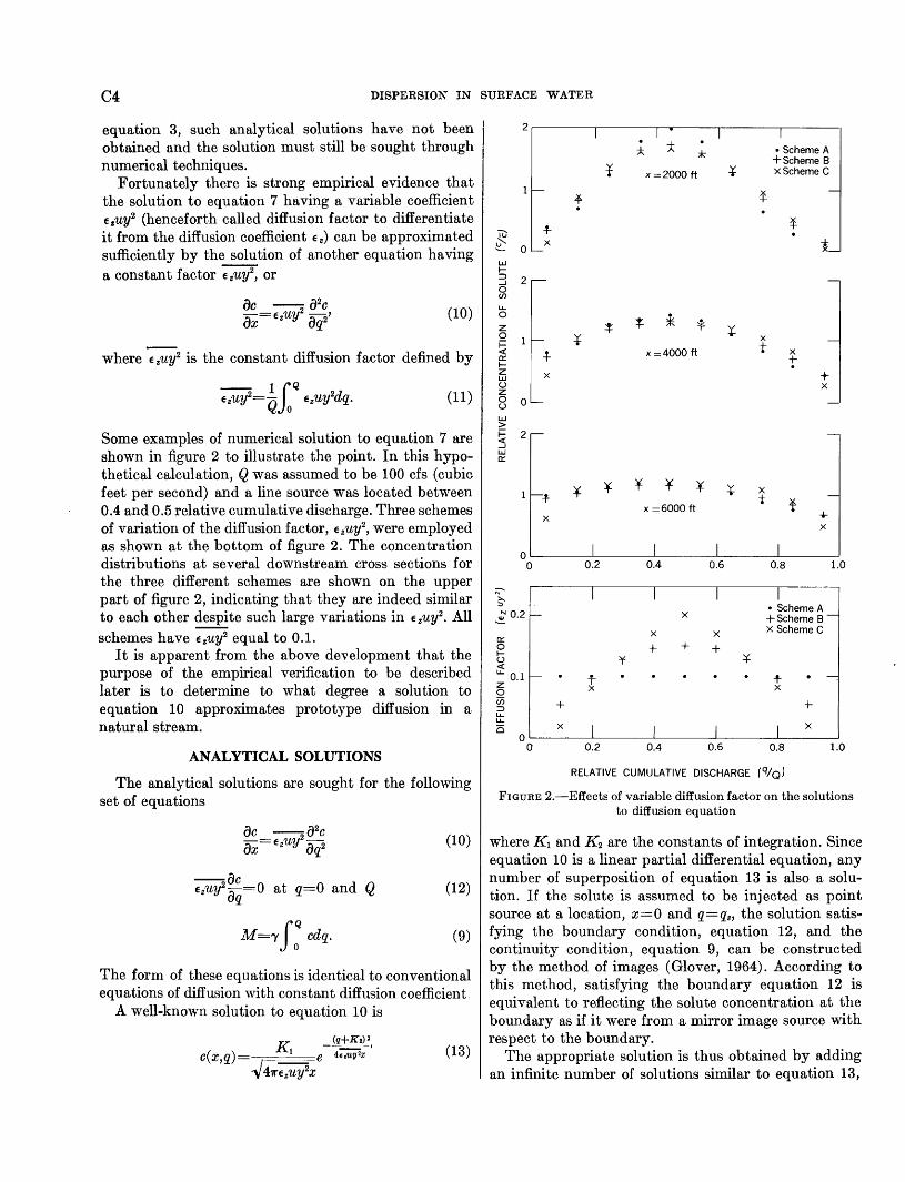
Some examples of numerical solution to equation 7 are shown in figure 2 to illustrate the point. In this hypo-thetical calculation, Q was assumed to be 100 cfs (cubic feet per second) and a line source was located between 0.4 and 0.5 relative cumulative discharge. Three schemes of variation of the diffusion factor, e2uy2

, were employed as shown at the bottom of figure 2. The concentration distributions at several downstream cross sections for the three different schemes are shown on the upper part of figure 2, indicating that they are indeed similar to each other despite such large variations in e2uy2

• All schemes have EzUY2 equal to 0.1.

It is apparent from the above development that the purpose of the empirical verification to be described later is to determine to what degree a solution to equation 10 approximates prototype diffusion rn a natural stream.

ANALYTICAL SOLUTIONS

The analytical solutions are sought for the following set of equations

(10)

--ac EzUY2 dq =0 at q=O and Q (12)

M=-r J: cdq. (9)

The form of these equations is identical to conventional equations of diffusion with constant diffusion coefficient.

A well-known solution to equation 10 is

(13)

2 . :!;:

* * • Scheme A

:r +Scheme 8 X =2000 ft -¥ X Scheme C

.ol' f-. f.

10 . ~ 0 i I.JJ f-::> 2 _, 0 en LL. 0 . z -* t * ~ ~ 0 1 -¥ X f= t <( X =4000 ft X a:: + f- . z I.JJ (..) z 0 0 (..)

I.JJ > f= 2 <( _, I.JJ a::

¥ ¥ ¥ ¥ ¥ -¥ X

X =6000 ft t t

X .... X

0 0 0.2 0.4 0.6 0.8 1.0

"' I I I I >-. :;:,

• Scheme A ~0.2 ~ X +Scheme 8-

X X x Scheme C 0::: + 0 + + f-(..) ¥ -¥ <(

LL. 0.1 - . + + . - . z X X 0 U5 + + ::> LL. LL.

C5 X I I I I X

0 0 0.2 0.4 0.6 0.8 1.0

RELATIVE CUMULATIVE DISCHARGE (q/Q)

FIGURE 2.-Effects of variable diffusion factor on the solutions to diffusion equation

where K1 and K 2 are the constants of integration. Since equation 10 is a linear partial differential equation, any number of superposition of equation 13 is also a solution. If the solute is assumed to be injected as point source at a location, x=O and q=q8 , the solution satisfying the boundary condition, equation 12, and the continuity condition, equation 9, can be constructed by the method of images (Glover, 1964). According to this method, satisfying the boundary equation 12 is equivalent to reflecting the solute concentration at the boundary as if it were from a mirror image source with respect to the boundary.

The appropriate solution is thus obtained by adding an infinite number of solutions similar to equation 13,


each solution representing the concentration from an actual source and successive image sources which come into play whenever the solute is reflected at the boundary. The series solution is written as

c(x,q)= Kl ± e- -- 4~~uY2x--[ {

(2nQ+q.-q) 2

"\147rEzUY2X n=O

(14)

In order to satisfy equation 9, equation 14 is integrated from q=O to Q and the result is equated to Mf'Y· The constant K 1 is fixed in this manner as

M Kl=--·

'Y

If the average concentration is defined by

- 1 fQ M c=Q)o cdq= 'YQ'

(15)

(16)

it will be more convenient to express the concentration cas a relative value to;. Also q and qs may be expressed as fractions of Q.

Equation 14 is thus reduced to the nondimensional form

af en { -~(2n+q',-q')Z c'(a,q')=- ~ e 2

.J2; n=O

where

+e -~'Cln+o'.+o'l'}

+ ± {e -~(2n-q',-q')2 n=l

a2 } +e 2 --(2n-q',+q')2 J

I C c =;;;;

c

(17)

(18)

(19)

(20)

and

(21)

It is useful to note that, as a consequence of normalization of variables and parameters, ff,c' dq' = 1. Equation 17 is similar to the solution obtained by Sayre and Chang (1968) through the time integration of an unsteady solution to the Fickian diffusion equation, which includes a time derivative term as well as a diffusion term in the longitudinal direction. Also, equation 21 is the nondimensional parameter used by Sayre (1965). Sayre's developments, however, are for a rectangular channel flow and use a different set of variables and constants.

When the solute is injected as a line source, the new solution may be constructed by the superposition of the point source solution, equation 17. Let the line source be located between q' s1 and q' s2 (q' s2>q' si) and assume that it consists of m point sources equally spaced at q' s~, q' s1 +Aq' s, q' s1 +2Aq' s, ... , q' s1 + (m-2)Aq' s, and q' s2· If the solute injection rate isM for all sources combined, each point source will produce the concentration distribution which is 1/m times equation 17, which, however, is adjusted for each source location. The superposition of all concentration distribution from the m sources will yield, for example, an expression corresponding to the first term of equation 17 such as

a ± {:i:_!_e -~(q'11+(i-1)..:1q',+2n-q')2} •

.J2~=o i=lm

B b . . 1 Aq~ d . . y su stitutmg , , +A , an Increasing m to m qs2-qsl qs

infinity and reducing Aq' s to zero at the same time, the above term is reduced to a limit form

(22)

By repeating a similar superposition and limit process to all other terms appearing in equation 17, the solution for a line source is finally obtained as


When diffusion is complete and the concentration, c, is uniform across the channel, P m attains the value of unity. The definition is compatible with the principle of mass continuity and is easily calculated from the plot of nondimensional concentration c(C against nondimensional cumulative discharge q/Q. Since the transverse distribution of solute is analytically determined as a function of a, q;t' q' s2' and q', the cross-sectional degree of mixing, P m' can likewise be determined analytically. This relation between P m and a, q;t' and q;2 is discussed later in connection with the estimation of mixing distances.

PROCEDURE FOR VERIFICATION BY STREAM (23) DATA

where erf designates the error function defined by

2 rq erf q= .J;Jo e-P 2dp,

and q;2 and q;1 are two end points of the line source expressed as fractions of total discharge Q. Equation 23 is again similar to the solution obtained by Sayre (1970) by the convolution of the point source solution with a line input function. It is also noted that equation 23

is normalized and !a1

c' dq' = 1·

Parameters representing the progress of transverse diffusion are used frequently in the following sections. One is the parameter a defined in equation 21. Even though this parameter is obtained by converting to nondimensional terms the parts of equation 14, its meaning is clear if it is noted that 2 E2'1ty2 x is approximately equal to the variance, u:, of the transverse solute distribution which is obtained in a channel without transverse boundaries and that equation 21 is reduced accordingly to

(21)

As the distance x increases, the time xj U increases and so does u:. Therefore a decreases as the distance increases and the diffusion becomes more complete as the result of solute reflection at boundaries.

The degree of mixing, P m' originally defined as percent mixing by E. D. Cobb and J. F. Bailey (written commun., 1965), may be written as

where

- 1 rQ c=Q )o cd.q

(24)

(16)

The procedure for testing the theoretical model by stream data consisted of (1) seeking and obtaining the best matching analytical solution to cross sectional data in terms of transverse solute distribution and degree of mixing, P m' (2) computing EzUY2 from the equation

(21)

(3) examining the consistency of computed EzUY2 for all cross sections used in a particular test, (4) computing the average diffusion coefficient E z by

--2 E =EzUY

z uy2 (25)

where the averaging means discharge weighting as defined in equation 11, and finally, (5) comparing the values of E z with Elder's formula as well as with values determined by other methods independent of the present model. The results are presented as a table of computed values of EzUY2 and Ez, and a graphic comparison of observed versus theoretical solute concentration distributions.

SOUTH RIVER TEST

The first verification study was made on the South River just upstream from the town of Waynesboro, V a. Three separate tests were made at this site. The reach was 2,300 feet long with a few very slight bends. The upper 1,000 feet of the reach was characterized by a large pool followed by two small riffies immediately downstream from the pool. The streambed was primarily sand and gravel with a few cobbles and larger rocks. There were a number of water-plant clumps in the reach. The stream width varied from about 40 to 80 feet with a mean width of about 60 feet. The average depth was from 1.0 to 1.5 feet. The flow during the study varied from 50 to 58 cfs. The average velocity in


the upper 1,200 feet of the reach was about 0.8 fps (feet per second), while that in the lower 1,100 feet was about 0.6 fps.

The solute used for the study was a fluorescent dye, Rhodamine WT. For the first test, the dye was injected continuously at the center of the stream by an airpowered, spring-diaphragm-regulated constant-rate injection unit. Once the dye entered the stream, a cross current in the channel caused the dye to flow toward the right bank. The stream was sampled at four downstream cross sections located at 800, 1,200, 1,600, and 2,000 feet from the injection site. Ten evenly spaced points were sampled at each cross section; three successive samples were obtained at each point.

The dye was injected for the second and third tests at a site 1,000 feet downstream from the first injection site to avoid the effect of the pool and riffles mentioned earlier. The same constant-rate-injection unit was used. In the second test, the dye, injected at the center of the channel, moved toward the left bank. In the third test the dye was injected at one-quarter of the width of the stream from each bank, the flow rate of the dye solution being approximately split between the two points. Samples for the second and third tests were obtained at cross sections located 400, 600, 1,000, and 1,290 feet downstream from the injection site. Sampling was done in a manner similar to sampling in the first test. Velocity and depth data were obtained at each sampling point by the standard current-meter method of the U.S. Geological Survey.

The concentrations of Rhodamine WT in the samples were determined by a Turner model 111 fluorometer after the samples were stored a few days to allow for the settling of sediment and adjusting to room temperature. All concentrations were temperature corrected as necessary and adjusted for effective background concentrations. The average concentration of the three samples obtained at each point was considered representative of that point. The degree of mixing P m and the cross-sectional average concentration c were computed at each cross section by equations 24 and 16.

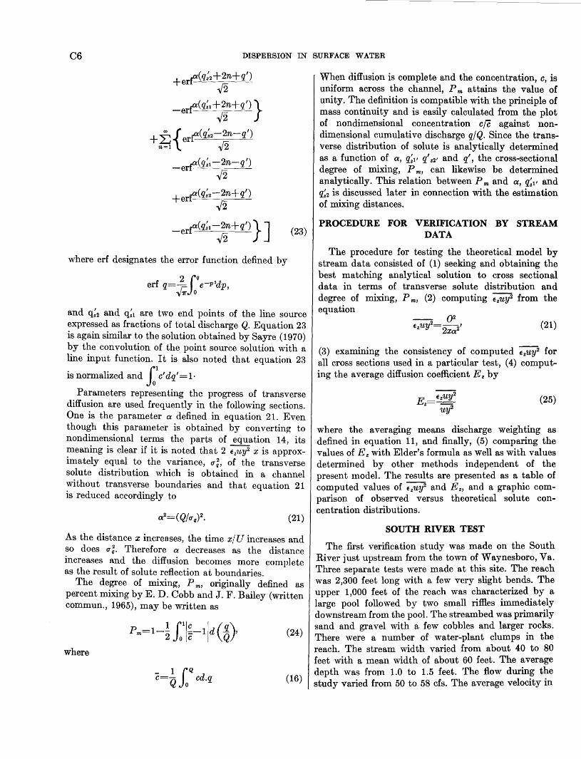
All concentration data are presented graphically in figures 3, 4, and 5. Since the relative concentration c' is computed by discharge weighting, the area underneath each distribution curve is unity and is directly comparable with theoretical solutions. To find the bestfit solution, however, a theoretical source location must be matched to the actual source location. Since the data included only geometric information of the source and not qs', the matching was accomplished empirically. Each observed distribution, c' vs q', was compared with several theoretical solutions, c' vs q', having the same degree of mixing, P m' as the data but having different source locations, q/. A representative qs' was

selected as giving the overall best-fit among all cross sections for a particular run. On the basis of this common source location, the best-fit theoretical solution for each cross section was taken as having the same degree of mixing as the data. These theoretical solutions are superimposed on the data in figures 3, 4, and 5. The agreement between the theoretical curves and the data points is satisfactory in most cross sections.

1.3 .-------.----r--,-----.----.--~-y-------,.--,..----,

1.1

1.0

0.8

1.2

1.1

~ '<- 1.0 z 0 f= 0.9 <( c:: f-

t5 0.8 ~ .. 0 () 1.2 LLJ > ~ 1.1 ...J LLJ c::

1.0

0.9

0.8

1.2

1.1

1.0

0.9

• Observed

-Theoretical

X =800ft

x= 1200 ft

x=1600ft

•

0.1 0.2 0.3 0.4 0.5 0.6 0.7 0.8 0.9 1.0

RELATIVE CUMULATIVE DISCHARGE (q!Q)

FIGURE 3.-Comparison of observed and theoretical concentration distribution, South River test 1

The data plotted by discharge weighting as used in this report present a much clearer picture of diffusion than do the data plotted by conventional distance weighting (c' vs z'=z/B). The data of test 2 are presented as examples in figure 6. The cross-sectional


• Observed

-Theoretical

il, ~1 z 0 ~ <( 0:: I-

0 -z w () 2 z 0 ()

w > ~ <(

1 ....J w 0::

o~~--~--~--~---L--~---L--~--.....1-~ 0 0.1 0.2 0.3 0.4 0.5 0.6 0.7 0.8 0.9 1.0

RELATIVE CUMULATIVE DISCHARGE' (q!Q)


average c based on distance weighting fluctuates a great deal from section to section, while that based on discharge weighting remains fairly steady. The degree of mixing also tends to be less consistent when it is based on the c' vs z' plot than when it is computed from c' vs q' plot. Furthermore, the transverse location of the peak concentration in the c' vs z' plot fluctuates between z' =0.2 to 0.5, while in the c' vs q' plot it remains steady at about q' =0.35. It is obvious from the velocity data that the meandering of high velocity threads caused irregular shifting of the peak in the c' vs z' plot while it produced no similar effect on the c' vs q' plot. These and other similar plottings confirmed that the c' vs q' plot that Cobb and Bailey proposed is sound from the concept of mass continuity and is also appropriate for the nondimensional presentation of natural stream data. Since the location of the peak concentration normally corresponds to the location of the source, the

0

2

~1 ~

z 0 ~ <( 0:: 0 I-z w ()

6 2 ()

w > ~ <( ....J

~ 1

0

2

• Observed

-Theoretical

o~~--~--~---L---L--~---L--~--.....1-~

0 0.1 0.2 0.3 0.4 0.5 0.6 0.7 0.8 0.9 1.0

RELATIVE CUMULATIVE DISCHARGE (q!Q)


representative source location determined from the plot of c' vs q' was considered to be the most reliable.

After the best-fit theoretical solution was chosen for a particular cross-section, the value of diffusion factor e2uy2 was computed by equation 21 from known values Q, x, and a, the last being determined from the bestfit solution. Before computing the average diffusion coefficient Ez by equation 25, the effective value of ·uy2 for the cross section was determined by weighting each upstream cross-sectional uy2 by appropriate longitudinal distance. Such weighting was necessary because the stream was not uniform and the observed diffusion pattern represented the sum effe.£!_ of the nonuniformity. The cross-sectional value of uy2 varied from 0.9 ft3 per sec at the middle of the reach to 4.0


2

0

2

lv ~ - 1 z 0 ;:::::: <X: a:: I-

~ 0 u a 2 u w > ;::::::

::5 ~ 1

0 2

\ \ ~ .......

............... -..

o~~--~--~--~--~--~--~--~~--~ 0 0.1 0.2 0.3 0.4 0.5 0.6 0.7 0.8 0.9 1.0

TRANSVERSE COORDINATE (ZfB or q/Q)

FIGURE 6.·-Comparison of concentration-transverse distance curve and concentration-cumulative discharge curve, South River test 2-

toward the end of the 2,300-foot long reach. The values of the pertinent parameters as well as the calculated Ez are tabulated in table 1. The consistency of Ez is satisfactory except in the first cross section of both test 1 and 2, where the values of P m show some anomaly. With an average Ez for tests 2 and 3 of 0.05 ft2 per sec, the calculated constant of Elder's formula is about 0.3 based on the estimate that u* is 0.13 fps and Dis 1.3 feet in this particular reach. On the other hand, Ez for test 1 is about three times the value of Ez for tests 2 and 3. Undoubtedly this represents a composite effect of high diffusion in the pool and riffles of the upper reach and less intense mixing in the lower reach. Since the theory does not accommodate such abrupt change of diffusion characteristic in the reach, test 1 should not be considered part of the verification. Nevertheless, the information is of considerable interest. Examination of figures 4 and 5 and table 1 shows that the verification of the theory by this set of tests is satisfactory.

ATRISCO FEEDER CANAL TEST

The second set of data used for verification was from diffusion tests on the Atrisco Feeder Canal near Bernalillo, about 15 miles north of Albuquerque, N. Mex. Part of the data was published and discussed by Fischer (1967b) and Yotsukura (1968). The present analysis, however, will examine all of the data. The study reach on this canal was much more uniform than that of the South River and had a straight alinement for about 12,000 feet. The stream cross section had a nearly rectangular shape for the entire length. The bed consisted of sand dunes, approximately 10 feet long and 0.8 to 1 foot high. The stream width varied from about 51 to 65 feet with an average width of about 60 feet. The average depth in the reach was about 2.2 feet, the mean velocity was 2.2 fps, and the discharge during the study varied from 255 cfs to 269 cfs.

TABLE !.-Computation of best-fit transverse diffusion coefficients, South River

Test Date z', q', Q (cfs) X (ft) Pm a ";.Uyi ;;yr E. (fV per sec2) (ft3 per sec) (ft2 per sec)

1 June 8, 1966 0. 5 0. 75 58 800 0. 934 1. 60 0. 821 3. 3 0.249 1,200 . 936 1. 58 . 561 3.4 . 165 1, 600 . 944 1. 53 . 449 3.0 . 150 2,000 . 949 1. 50 . 374 2. 7 . 139

2 June 9, 1966 0. 5 0.35 54 400 . 781 3. 63 . 277 2. 9 . 096 600 . 735 4.40 . 126 2.4 . 053

1,000 . 771 3. 80 . 101 2.0 . 051 1, 290 . 829 2.97 . 128 2. 2 . 058

3 June 9, 1966 0. 25 0. 10 50 400 . 825 4. 62 . 146 2.9 . 050 and and 600 . 872 3.98 . 132 2.4 . 055

0. 75 0.85 1,000 . 921 3. 37 . 110 2. 0 . 055 1,290 . 944 3.09 . 101 2. 2 . 046

4-66-743 0-72~2

ClO DISPE'RSION IN SURFACE WATER

Rhodamine WT dye was injected at a constant rate into the stream by a Mariotte constant-head tank. For the first and second tests, the dye was injected at the center of the stream; whereas, for the third test, it was injected at a point 1 foot from the left bank. The stream was sampled at eight to ten cross sections, located between 200 and 6,500 feet downstream from the injection site. All samples in a cross section were obtained simultaneously by submerging a set of 24 milliliter vials suspended from a nylon cord stretched across the channel. The vials were spaced at a uniform interval of 2 feet. Velocity data were obtained at every sampling cross section within 1,200 feet from the injection site, but only at a few sections further downstream. Depth data were obtained at each sampling section. A more detailed description of the study reach and the test procedure was given by Fischer (1967b).

The concentrations of the samples were determined in a manner similar to that for the South River data. Since only one sample was obtained at each point, the concentration of that sample was considered steadystate concentration at that point. The procedure of data analysis was the same as for the South River data.

The results of tests are given in figures 7, 8, and 9, and table 2. Several cross-sectional data from test 3 (side injection test) are not presented because the deviations of the computed c for these sections were more than 10 percent of the average c of all cross sections and were considered excessive for solute mass continuity. The error in c for the side injection test tends to be large relative to the error inc for the midstream injection, because the high solute concentration which contributes heavily to c, is in the region of slow bank-side flow where velocity and its measurement tend to be erratic. The source location was determined as in the South River tests. For tests 1 and 2, however, velocity measurements made within 50 feet of the injection site indicate that, at the center of the channel where the injection nozzle was located, the relative cumulative discharge from the left bank, q/, was about 0.45, which agrees well with the value determined from the concentration data.

The agreement of observed and theoretical solute distributions appears quite satisfactory. The theoretical distributions are based on the best matching values of q' s and a (P m) tabulated in table 2. Especially noticeable is the result that the solute distributions at distances less than 1,000 feet from the injection site show typical Gaussian pattern. Comparison of such distributions with the typically skewed distributions of the plot, c' vs z', again demonstrated that the present analytical approach using the cumulative discharge q' as the transverse variable is indeed com-

patible with the conditions in natural streams. In this connection, the equation relating the variance of the

TU .:;-...

z 0 t= <( a:: 1-z UJ u z 0 u UJ > t= <( _J

UJ a::

2

0 2

0

X =800ft

X =3200 ft

i i • • • •x~~=== •I• J 1.0 0.2 0.3 0.4 0.5 0.6 0.7 0.8 0.9 1.0

RELATIVE CUMULATIVE DISCHARGE. (q!Q)

FIGURE 7.-Comparison of observed and theoretical concentration distribution, Atrisco Feeder Canal test 1

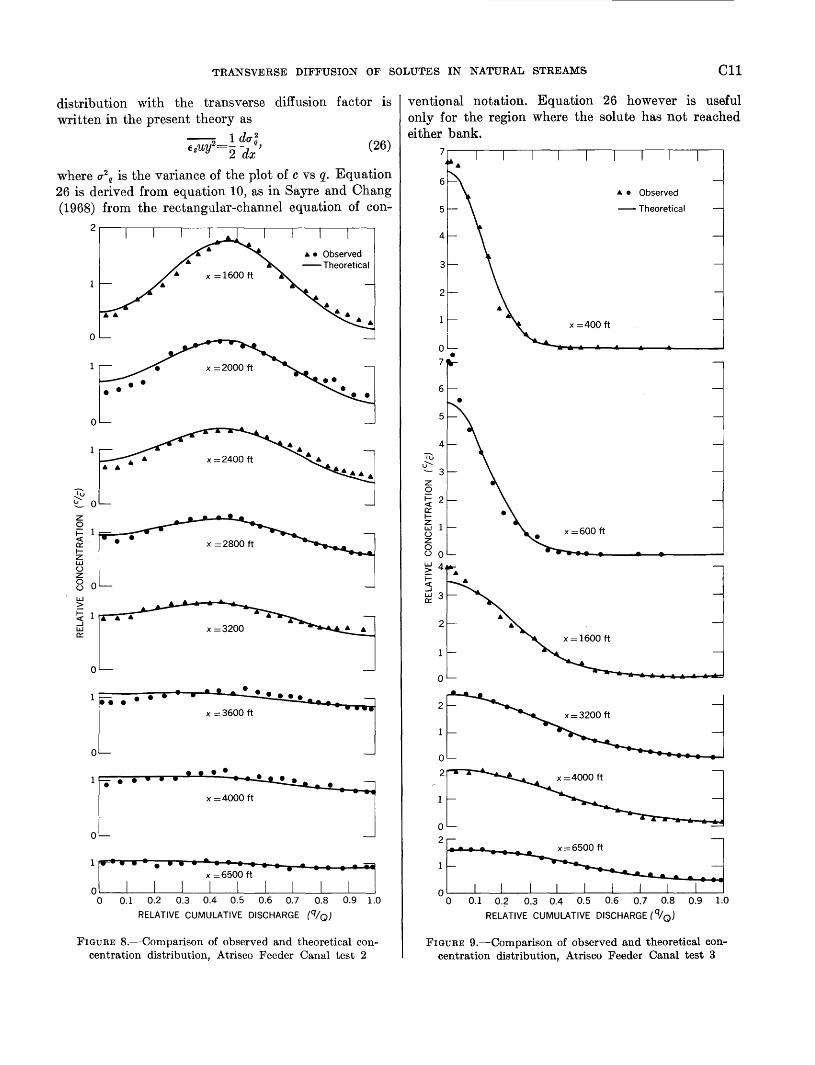
TRANSVERSE DIFFUSION OF SOLUTES IN NATURAL STREAMS Cll

distribution with the transverse diffusion factor is written in the present theory as

(26)

where u 2 q is the variance of the plot of c vs q. Equation 26 is derived from equation 10, as in Sayre and Chang (1968) from the rectangular-channel equation of con-

~ ;:;..:

z 0 i= <( a:: I-z w (.) z 0 (.)

w > i= <( _J

w a::

2.---.---.---~---r---.--~--~~------.-~

0

0

8 e I • ••• . ..... J I W W

:r • • • • •

X =3600 ft

• • • • •

1r······~······~····· X =6500 ft

0 I I I I I I 0 0.1 0.2 0.3 0.4 0.5 0.6 0.7 0.8

RELATIVE CUMULATIVE DISCHARGE (qiQ)

FIGURE B.-Comparison of observed and theoretical concentration distribution, Atrisco Feeder Canal test 2

ventional notation. Equation 26 however is useful only for the region where the solute has not reached either bank.

z 0 i= <( a:: I-z w (.) z 0 (.)

w > i= <( _J

w a::

7,---,---.---.---.---.---~---.---,---.--~

6

5

4

3

2

2

0 4

3

2

0

2

X =400ft

• • Observed

- Theoretical

0

2

1 ~ 0

- x-6500 ft l [ ~ .. ~----.........~. ·, ·~·~· ~ 0 0.1 0.2 0.3 0.4 0.5 0.6 0.7 0.8 0.9 1.0


FIGURE 9.-Comparison of observed and theoretical concentration distribution, Atrisco Feeder Canal test 3


TABLE 2.-Computation of best-fit transverse diffusion coefficients, Atrisco Feeder Canal

Test Date z', q', Q (cfs)

1 June 21, 1966 0. 5 0.4 269

2 June 22, 1966 0. 5 0.45 258

3 June 23, 1966 0. 0 0. 0 263

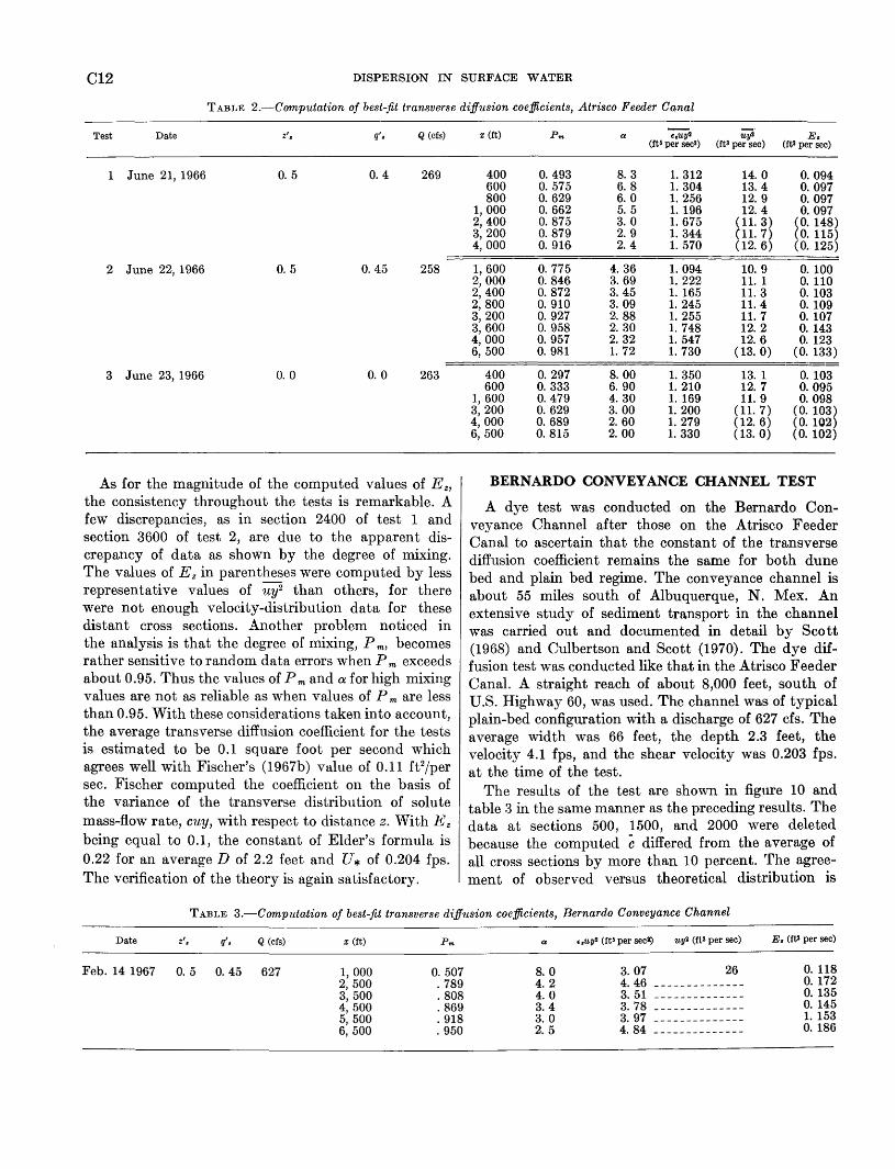
As for the magnitude of the computed values of Ez, the consistency throughout the tests is remarkable. A few discrepancies, as in section 2400 of test 1 and section 3600 of test 2, are due to the apparent discrepancy of data as shown by the degree of mixing. The values of Ez in parentheses were computed by less representative values of uy2 than others, for there were not enough velocity-distribution data for these distant cross sections. Another problem noticed in the analysis is that the degree of mixing, P m' becomes rather sensitive to random data errors when P m exceeds about 0.95. Thus the values of P m and a for high mixing values are not as reliable as when values of P m are less than 0.95. With these considerations taken into account, the average transverse diffusion coefficient for the tests is estimated to be 0.1 square foot per second which agrees well with Fischer's (1967b) value of 0.11 ft2/per sec. Fischer computed the coefficient on the basis of the variance of the transverse distribution of solute mass-flow rate, cuy, with respect to distance z. With Ez being equal to 0.1, the constant of Elder's formula is 0.22 for an averageD of 2.2 feet and U* of 0.204 fps. The verification of the theory is again satisfactory.

·-----------------X (ft) Pm a E,uy2 uy;· E,

(ft3 per sec2) (ft3 per sec) (ft2 per sec)

400 0.493 8. 3 1. 312 14. 0 0. 094 600 0. 575 6. 8 1. 304 13.4 0.097 800 0.629 6. 0 1. 256 12. 9 0. 097

1,000 0. 662 5. 5 1. 196 12.4 0. 097 2,400 0.875 3. 0 1. 675 (11.3) (0. 148) 3, 200 0.879 2. 9 1. 344 (11. 7) (0. 115) 4, 000 0. 916 2.4 1. 570 ( 12. 6) (0. 125)

1,600 0. 775 4. 36 1. 094 10. 9 0. 100 2,000 0. 846 3. 69 1. 222 11. 1 0. 110 2,400 0. 872 3.45 1. 165 11. 3 0. 103 2,800 0. 910 3. 09 1. 245 11. 4 0. 109 3, 200 0. 927 2. 88 1. 255 11. 7 0. 107 3, 600 0. 958 2. 30 1. 748 12. 2 0. 143 4,000 0. 957 2. 32 1. 547 12.6 0. 123 6, 500 0. 9Rl 1. 72 1. 730 ( 13. 0) (0. 133)

400 0. 297 8. 00 1. 350 13. 1 0. 103 600 0. 333 6. 90 1. 210 12. 7 0.095

1, 600 0.479 4. 30 1. 169 11. 9 0. 098 3, 200 0. 629 3. 00 1. 200 (11. 7) (0. 103) 4,000 0. 689 2. 60 1. 279 (12. 6) ( 0. 102) 6, 500 0. 815 2.00 1. 330 ( 13. 0) (0. 102)

BERNARDO CONVEYANCE CHANNEL TEST

A dye test was conducted on the Bernardo Conveyance Channel after those on the Atrisco Feeder Canal to ascertain that the constant of the transverse diffusion coefficient remains the same for both dune bed and plain bed regime. The conveyance channel is about 55 miles south of Albuquerque, N. Mex. An extensive study of sediment transport in the channel was carried out and documented in detail by Scott (1968) and Culbertson and Scott (1970). The dye diffusion test was conducted like that in the Atrisco Feeder Canal. A straight reach of about 8,000 feet, south of U.S. Highway 60, was used. The channel was of typical plain-bed configuration with a discharge of 627 cfs. The average width was 66 feet, the depth 2.3 feet, the velocity 4.1 fps, and the shear velocity was 0.203 fps. at the time of the test.

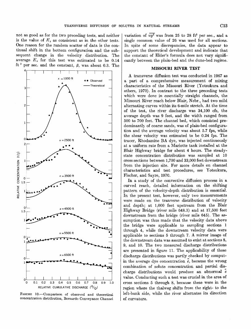
The results of the test are shown in figure 10 and table 3 in the same manner as the preceding results. The data at sections 500, 1500, and 2000 were deleted because the computed c differed from the average of all cross sections by more than 10 percent. The agreement of observed versus theoretical distribution is

TABLE 3.-Computation of best-fit transverse diffusion coefficients, Bernardo Conveyance Channel

Date z', q'. Q (cfs) X (ft) Pm a E,uy2 (ft5 per sect) uy2 (fta per sec) E. (ft2 per sec)

Feb. 14 1967 0. 5 0. 45 627 1,000 0. 507 8. 0 3. 07 26 0. 118 2, 500 . 789 4. 2 4.46 -------------- 0. 172 3, 500 . 80R 4. 0 3. 51 -------------- 0. 135 4, 500 . 869 3.4 3. 78 ------- 0. 145 5, 500 . 918 3. 0 3. 97 -------------- 1. 153 6, 500 . 950 2. 5 4. 84 -------------- 0. 186


not as good as for the two preceding tests, and neither is the value of E z as consistent as in the other tests. One reason for the random scatter of data is the continual shift in the bottom configuration and the subsequent change in the velocity distribution. The average Ez for this test was estimated to be 0.14 ft 2 per sec. and the constant, {1, was about 0.3. The

:@ ~

z 0 i= <( a:: 1-z UJ () z 0 ()

UJ > i= <( _J

UJ a::

4.--.---,---,--~--~--~--~~--~--~

2

0

2

0 1.5

0 1.5

X = 1000 ft

X =2500 ft

• • Observed

-Theoretical

I 0.1 0.2 0.3 0.4 0.5 0.6 0.7 0.8 0.9 1.0


FIGURE 10.-Comparison of observed and theoretical concentration distribution, Berna.rdo Conveyance Channel

variation of 11.y2 was from 25 to 28 ft3 per sec., and a single common value of 26 was used for aH sections. In spite of some discrepancies, the data appear to support the theoretical development and indicate that the constant of Elder's formula does not vary significantly between the plain-bed and the dune-bed regime.

MISSOURI RIVER TEST

A transverse diffusion test was conducted in 1967 as a part of a comprehensive measurement of mixing characteristics of the Missouri River (Yotsukura and others, 1970). In contrast to the three preceding tests which were done in essentially straight channels, the Missouri River reach below Blair, Nebr., had two mild alternating curves within its 6-mile stretch. At the time of the test, the river discharge was 34,100 cfs, the average depth was 9 feet, and the width ranged from 500 to 700 feet. The channel bed, which consisted predominantly of coarse sands, was of plain-bed configuration and the average velocity was about 5.7 fps, while the shear velocity was estimated to be 0.24 fps. The tracer, Rhodamine BA dye, was injected continuously at a uniform rate from a Mariotte tank installed at the Blair Highway bridge for about 4 hours. The steadystate concentration distribution was sampled at 10 cross sections between 1,700 and 33,000 feet downstream from the injection site. For more details on channel characteristics and test procedures, see Yotsukura, Fischer, and Sayre, 1970.

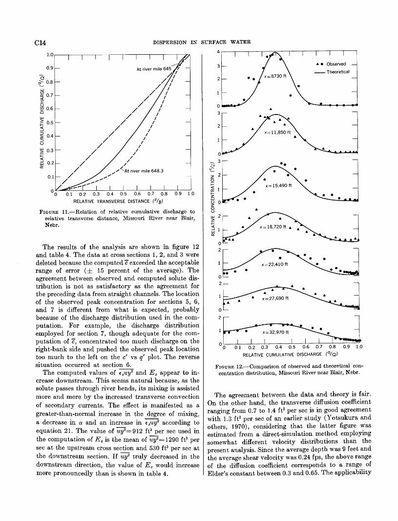
In a study of the convective diffusion process in a curved reach, detailed information on the shifting pattern of the velocity-depth distribution is essential. In the present test, however, only two measurements were made on the tranverse distribution of velocity and depth; at 1,000 feet upstream from the Blair Highway Bridge (river mile 648.3) and at 17,500 feet downstream from the bridge (river mile 645). The assumption was thus made that the velocity data above the bridge were applicable to sampling sections 1 through 4, while the downstream velocity data were applicable to sections 5 through 7. A mirror image of the downstream data was assumed to exist at sections 8, 9, and 10. The two measured discharge distributions are presented in figure 11. The applicability of these discharge distributions was partly checked by computin the average dye concentration c, because the wrong combination of solute concentration and partial discharge distributions would produce an abnormal c value. Conducting such a test was crucial in the area of cross sections 5 through 8, because these were in the region where the thalweg shifts from the right- to the left-bank side, while the river alternates its direction of curvature.


0.9

a ;;:- 0.8 -

l.LJ

~ 0.7 <( I (.)

~ 0.6 Cl

l.LJ

~ 0.5 ::5 ~ 0.4 :::> (.)

~ 0.3 ;::: <( _J

l.LJ 0::

0.1 0.2 0.3 0.4 0.5 0.6 0.8

RELATIVE TRANSVERSE DISTANCE (z/8)

FIGURE H.-Relation of relative cumulative discharge to relative transverse distance, Missouri River near Blair, Nebr.

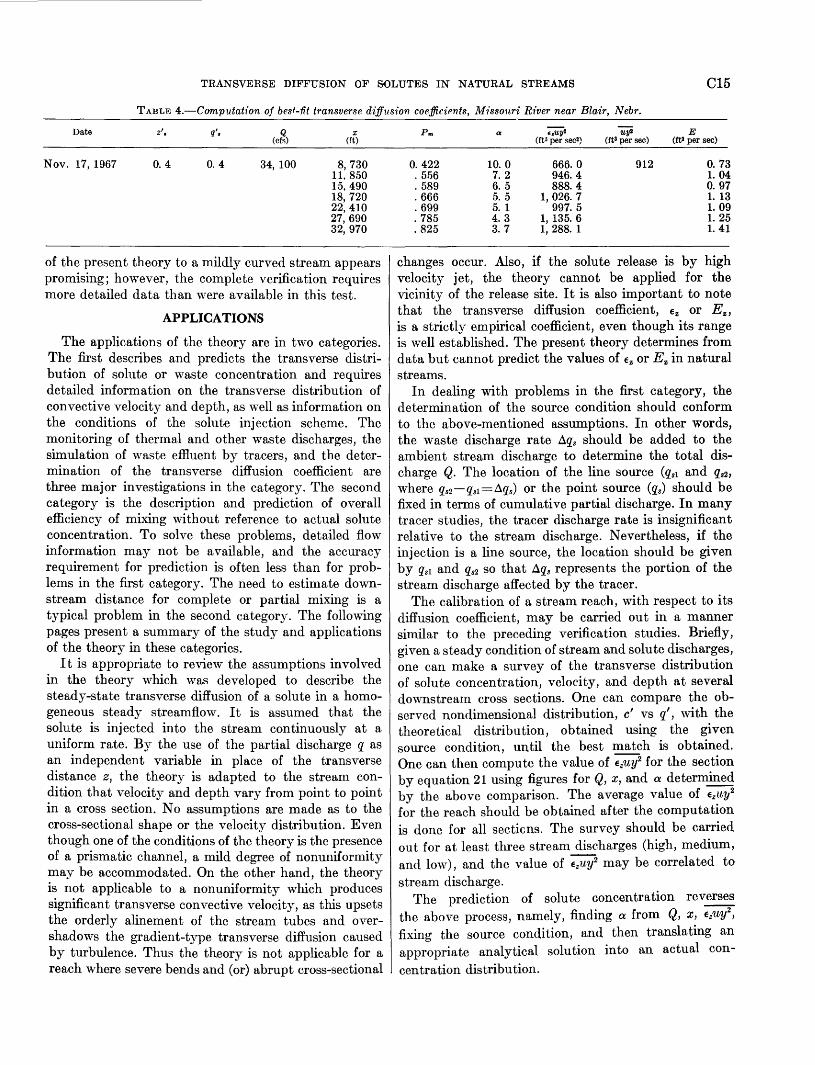
The results of the analysis are shown in figure 12 and table 4. The data at cross sections 1, 2, and 3 were deleted because the computed c exceeded the acceptable range of error ( ± 15 percent of the average). The agreement between observed and computed solute distribution is not as satisfactory as the agreement for the preceding data fron1 straight channels. The location of the observed peak concentration for sections 5, 6, and 7 is different from what is expected, probably because of the discharge distribution used in the computation. For example, the discharge distribution employed for section 7, though adequate for the computation of c, concentrated too much discharge on the right-bank side and pushed the observed peak location too much to the left on the c' vs q' plot. The reverse situation occurred at section 6.

The computed values of e2uy2 and Ez appear to increase downstream. This seems natural because, as the solute passes through river bends, its mixing is assisted more and more by the increased transverse convection of secondary currents. The effect is manifested as a greater-than-normal increase in the degree of mixing, a decrease in a and an increase in e zUY2 according to equation 21. The value of uy2=912 ft3 per sec used in the computation of E z is the mean of uy2= 1290 ft3 per sec at the upstream cross section and 530 ft3 per sec at the downstream section. If uy2 truly decreased in the downstream direction, the value of E z would increase more pronouncedly than is shown in table 4.

4·~~--~--~--~---.---.---r---,--,---,

3 A • Observed

2

2

IU 3

~ z 2 0 ;::: <(

1 0:: I-z l.LJ (.) 0 z 0 A (.)

l.LJ 2 > ;::: <(

w::l 1 0::

0 2

• x=22,410 ft

0 2

• x=27,690 ft

0

FIGURE 12.-Comparison of observed and theoretical concentration distribution, Missouri River near Blair, Nebr.

The agreement between the data and theory is fair. On the other hand, the transverse diffusion coefficient ranging from 0. 7 to 1.4 ft2 per sec is in good agreement with 1.3 ft2 per sec of an earlier study (Yotsukura and others, 1970), considering that the latter figure was estimated from a direct-simulation method employing somewhat different velocity distributions than the present analysis. Since the average depth was 9 feet and the average shear velocity was 0.24 fps, the above range of the diffusion coefficient corresponds to a range of Elder's constant between 0.3 and 0.65. The applicability


TABLE 4.-Computat1'on of besf-fit transver.c;e diffusion coefficif>nts, M1'ssouri R1'ver near Blair, Nebr.

Date z', q'. Q X (cfs) (ft)

Nov. 17, 1967 0.4 0. 4 34, 100 8, 730 11. 8.50 15,490 18, 720 22,410 27,690 32, 970

of the present theory to a mildly curved stream appears promising; however, the complete verification requires more detailed data than were available in this test.

APPLICATIONS

The applications of the theory are in two categories. The first describes and predicts the transverse distribution of solute or waste concentration and requires detailed information on the transverse distribution of convective velocity and depth, as well as information on the conditions of the solute injection scheme. The monitoring of thermal and other waste discharges, the simulation of waste effluent by tracers, and the determination of the transverse diffusion coefficient are thrHe major investigations in the category. The second category is the description and prediction of overall efficiency of mixing without reference to actual solute concentration. To solve these problems, detailed flow information may not be available, and the accuracy requirement for prediction is often less than for problems in the first category. The need to estimate downstream distance for complete or partial mixing is a typical problem in the second category. The following pages present a summary of the study and applications of the theory in these categories.

It is appropriate to review the assumptions involved in the theory which was developed to describe the steady-state transverse diffusion of a solute in a homogeneous steady streamflow. It is assumed that the solute is injected into the stream continuously at a uniform rate. By the use of the partial discharge q as an independent variable in place of the transverse distance z, the theory is adapted to the stream condition that velocity and depth vary from point to point in a cross section. No assumptions are made as to the cross-sectional shape or the velocity distribution. Even though one of the conditions of the theory is the presence of a prismatic channel, a mild degree of nonuniformity may be accommodated. On the other hand, the theory is not applicable to a nonuniformity which produces significant transverse convective velocity, as this upsets the orderly alinement of the stream tubes and overshadows the gradient-type transverse diffusion caused by turbulence. Thus the theory is not applicable for a reach where severe bends and (or) abrupt cross-sectional

Pm a E,uy2 uy2 E (fts per sec2) (ft3 per sec) (ft2 per sec)

0. 422 10.0 666. 0 912 0. 73 . 5.56 7. 2 946.4 1. 04 . 589 6. 5 888.4 0. 97 . 666 5. 5 1,026. 7 1. 13 . 699 5. 1 997.5 1. 09 . 785 4. 3 1, 135. 6 1. 25 . 825 3. 7 1, 288. 1 1. 41

changes occur. Also, if the solute release is by high velocity jet, the theory cannot be applied for the vicinity of the release site. It is also important to note that the transverse diffusion coefficient, Ez or Ez,

is a strictly empirical coefficient, even though its range is well established. The present theory determines from data but cannot predict the values of Ez or Ez in natural streams.

In dealing with problems in the first category, the determination of the source condition should conform to the above-mentioned assumptions. In other words, the waste discharge rate !::t.q8 should be added to the ambient stream discharge to determine the total discharge Q. The location of the line source (qsl and qs2, where q82 -qsl =!::t.q8) or the point source (qs) should be fixed in terms of cumulative partial discharge. In many tracer studies, the tracer discharge rate is insignificant relative to the stream discharge. Nevertheless, if the injection is a line source, the location should be given by qsl and q82 so that !::t.qs represents the portion of the stream discharge affected by the tracer.

The calibration of a stream reach, with respect to its diffusion coefficient, may be carried out in a manner similar to the preceding verification studies. Briefly, given a steady condition of stream and solute discharges, one can make a survey of the transverse distribution of solute concentration, velocity, and depth at several downstream cross sections. One can compare the observed nondimensional distribution, c' vs q', with the theoretical distribution, obtained using the given source condition, until the best match is obtained. One can then compute the value of EzUY

2 for the section by equation 21 using figures for Q, x, and a determined by the above comparison. The average value of Eztty

2

for the reach should be obtained after the computation is done for all secticns. The survey should be carried out for at least three strean1 discharges (high, medium, and low), and the value of EzU.Y2 may be correlated to stream discharge.

The prediction of solute concentration reverses the above process, namely, finding a from Q, x, EzUY

2,

fixing the source condition, and then translating an appropriate analytical solution into an actual concentration distribution.


The computation of the transverse diffusion coefficient, Ez, is not necessary for calibration and prediction. However, since the data of the transverse distribution of velocity and depth are parts of the survey, Ez can easily be computed by equation 25.

To estimate the mixing distance or efficiency, the simplest scheme uses the degree of mixing, P m' as defined previously. The analytical relation between P m and a was calculated for typical point- and linesource arrangements and is pre sen ted in figures 13 and 14. Along with the distance equation,

(21)

these figures can be used to estimate a relation between the distance x and the degree of mixing P m·

Noteworthy is the fact that the required distance x

E ~

0.9

(.!) 0.7 z x ~ LL. 0 LLJ

::::! 0.6 (.!) LLJ 0

0.5

0.4

for bank side injection (q;=O) is four times as long as distance for midstream injection (q;=0.5) to obtain the same degree of mixing. The premise can also be stated figuratively that a near-bank injection is equivalent to a midstream injection in the same channel with a discharge twice as large as the actual. Another premise of practical interest applies to multipoint sources. Assume that the channel is divided into N stream tubes of equal discharges, and the source is at the center of each stream tube. For this arrangement of N sources, the distance x necessary for a certain mixing level can be reduced to 1/N2 times the distance for a single midstream source.

Equation 21 can be further simplified as needed. Let the channel depth, D, be defined by

D~J.B ydz, B

(27)

DISTANCE PARAMETER (a)

FIGURE 13.-Theoretical relation of degree of mixing, P m. to distance parameter, a, and source location, q' ,, for point source injection


where B is the width at the water surface. Also the average U is defined

foBuydz Q U-- -=--·

fo B BD ydz

0

(28)

With these average quantities and equation 1 for the transverse diffusion coefficient, equation 21 is transformed to

1 UD2 U B 2

X=--·--·-·-· 2a2

{3 'UY2 u* D (29)

To use equation 29, two expressions, UD2juy 2 and 1/2a 2{3, need to be evaluated. The nondimensional ratio UD 2/uy 2 accounts for the deviation of flow and geometry of a natural stream from that of an idealized rectangular channel. The data tabulated in table 5

were obtained from the streams used for the vertification, and the ratio UD 2/uy 2 ranges from 0.3 to 0.9. As for the other expression 1/2a 2{3, {3 ranges from 0.2 to 0.3 for a straight channel but can go up to 0.6 for channels with mild bends. The value of a should be chosen from figures 13 and 14 if the conditions are known for Pm and q;.

The choice of a value for P m for so-called complete mixing depends on the nature of a particular study. For discharge measurements by dye dilution methods a mixing distance based on the value of P m of 98 percent is recommended because this mixing insures that the theoretical maximum deviation of concentration from the mean is about 3 percent. For less accurate predictions, a P m of 95 percent is adequate. In this connection, figures 13 and 14 indicate that the mixing distance is very sensitive to P m for high mixing values. For example, the distance required to improve the

1.0~-------=~------~--------.--------,--------.--------,,--------.--------,--------,

E ~

0.8

(.!l 0.7 z x ~ LJ.. 0 UJ

~ 0.6 (.!l UJ 0

0.5

DISTANCE PARAMETER (a)

FIGURE 14.-Theoretical relation of degree of mixing, P m' to distance parameter, a, and source location, q' •1 and q' d, for line source injections


TABLE 5.-Cross-sectional form parameter, UD2fuy2, of natural streams

Stream

South River; test L ____________ _ South River: tests 2 and 3 _______ _ Atrisco Feeder CanaL ___________ _ Bernardo Conveyance ChanneL __ _ Missouri River near Blair ________ _

B (ft)

60 60 60 66

600

D (ft)

1. 21 1. 44 2. 0 2.3

10. 0

mixing from 95 to 99.5 percent may be as much as the distance required to attain the initial mixing of 95 percent. On the other hand, such a theoretical result is difficult to verify by stream data, because as noted previously field measurements of P m often cannot attain sufficient accuracy.

The application of equation 29 has been tested with the data collected by Barsby, Delannoy, and Watt (1967) on mainly shallow mountain streams of straight alinement. The tracer was salt, the concentration of which was measured by conductance measurement. No data for transverse distribution of velocity and depth were collected. The comparison of observed and estimated m1x1ng distance 1s presented in table 6. The values for Q, B, D, U, and P m. are from the above report and U* is computed by -JgDS. In the estimate, it

u (ft per sec)

0. 8 .6

2. 2 4. 1 5. 7

Q (cfs)

58 52

263 627

34,100

UIJ2 (fta per sec)

1. 17 1. 24 8.8

21. 7 570

uy2 (ft3 per sec)

2. 7-3.4 2. 0-2. 9

11-14 26

912

0.43-0.35 . 62- . 43 . 80- . 63 . 83 . 62

was assumed that 13=0.23 and UD2fuy 2= 1, while a was obtained from figure 13, in which the value of P m was known.

The agreement between observed and estimated distance is fairly good for the Alwen River. For the Brenig, Wye, and Devon Rivers, the estimated x's are much larger than the observed values. This discrepancy is explained reasonably well by the possibility of UD2/uy2 being less than unity in these rivers. The discrepancy for the Whitewater River is probably due to this being the only stream with significant bends, thus, higher 13 values. On the other hand, the proposed equation does not apply at all to the Hambleden Brook.

The foregoing analysis, in comparison with the verification studies, demonstrates that mixing distance cannot be predicted with a high degree of accuracy unless

TABLE 6.-C omparison of estimated and observed mixing distances, Water Research Association data

Test River Q (cfs) B (ft) D (ft) U (fps)

1 Brenig ____________ _ 12. 1 21.4 0.8 0. 7

2 Alwen ____________ _ 8. 2 13. 5 0. 57 1. 07

3 Alwen ____________ _ 5. 3 12. 7 0. 5 0.84

4 Alwen ____________ _ 5. 3 13.4 0.47 0.84

5 Alwen _____________ _ 25.5 37. 0 0. 64 1.1

6a VVye ______________ _ 59.0 20.4 1. 15 2. 57

7 a Devon ____________ _ 170.0 40. 1 2. 1 2. 04

8 VVhi tewa ter _______ _ 17. 5 26. 6 1. 03 0. 64

9 Hambleden Brook __ _ 4. 6 7. 2 0. 83 0. 77

u. (fps)

0. 66

o. 33

0.44

0.30

0.48

0. 27

0.49

0. 27

0.46

Pm

0. 923 . 989

. 520 . 830 . 907 . 942

. 773

. 957

. 996

. 780 . 860 . 944 . 966

. 605

. 751

. 773 . 845 . 986

. 820 . 881 . 972 . 991

. 987 . 993 . 996

. 941

. 970

. 995

a

3.06 2. 18

7.80 3. 87 3. 20 2.86

4.36 2. 71 1. 95

4. 31 3. 61 2. 84 2. 60

6.29 4. 57

4.36 3. 74 2.27

3. 96 3.44 2. 51 2. 15

2. 25 2.08 1. 95

2.87 2. 55 2.00

Estimated X (ft)

141 278

37 150 220 275

70 183 352

125 178 28R 344

270 510

394 535

1,450

440 585

1, 100 1, 500

700 810 905

28 35 57

Observed :t (ft)

100 200

50 100 200 270

60 160 310

50 100 200 270

200 400

100 230 770

100 200 500 800

100 300 800

70 130 250


detailed information of channel geometry and velocity is available. Nonetheless, equation 29 is useful if the limitations of the formula are fully understood.

When the assumptions are that a=2.3, /3=0.23, and UD2juy2=0.6 for complete mixing resulting from a midstream injection, equation 29 is reduced to the simplest form

U B2

x=0.25 u*. n· (30)

Equation 30 is comparable to the formula derived by G. M. Rimmar (British Standards Institution, 1964)

B2 x=0.130z(0.70z+11) gD' (31)

where Oz is the Chezy coefficient of channel roughness. Equation 31 is written for the foot-pound-second system and is equivalent to assuming, in equation 29,

th t 2 UD2j-2-1 d f.l __ {g__ h R a a= , uy- , an fJ- (0.70z+ 11)' w ere fJ

ranges from 0.11 to 0.37, as Oz varies from 60 to 6. Both equations 30 and 31 are valid only for conditions of eomplete mixing of solutes by midstream injection in a straight channel.

CONCLUSIONS

The preceding section summarized the present study concerning application to practical problems. This section is devoted only to the essential conclusions derived frmn the field verifications of the proposed model. 1. The proposed model enables steady-state transverse

diffusion of solutes in natural streams to be described satisfactorily by analytical solutions of the diffusion equation. It is satisfactory insofar as present knowledge on transverse diffusion coefficients prescribes the use of a cross-sectional average value, Ez, rather than use of local values, Ez(z), in diffusion models.

2. The study established that the cumulative partial discharge, q, rather than the transverse distance, z, is the prime variable to be considered in transverse diffusion processes.

3. The model enables the reduction of transverse diffusion data in terms of nondimensional variables consistent with the mass balance of solutes in natural streams.

4. Calculated diffusion coefficients by the model are in good agreement with Elder's formula (/3=0.23) and are consistent within straight shallow reaches of a natural stream.

REFERENCES

Barsby, A., Delannoy, C., and Watt, J. P. C., 1967, River gaging by dilution techniques-!: Tech. Paper 58, Water Research Association, Buchinghamshire, England, 34 p.

British Standards Institution, 1964, Methods of measurement of liquid flow in open channels, Part 2A, dilution methods, constant rate inj~ction: British Standard 3680, 39 p.

Culbertson, J. K., and Scott, C. H., 1970, Sandbar development and movement in an alluvial channel: U.S. Geol. Survey Prof. Paper 700-B, p. B237-B241.

Elder, J. W., 1959, The dispersion of marked fluid in turbulent shear flow: Jour. Fluid Mechanics, v. 5, no. 4, p. 544-560.

Engelund, Frank, 1969, Dispersion of floating particles in uniform channel flow: Am. Soc. Civil Engineers, Jour. Hydraulics Div., v. 95, no. HY4, p. 1149-1162.

Fischer, H. B., 1967a, The mechanics of dispersion in natural streams: Am. Soc. Civil Engineers, Jour. Hydraulics Div., v. 93, no. H Y6, p. 187-216.

--- 1967b, Transverse mixing in a sand-bed channel: U.S. Geol. Survey Prof. Paper 575-D, p. D267-D272.

--- 1969, The effect of bends on dispersion in streams: Am. Geophysical Union, Water Resources Research, v. 5, no. 2, p. 496-506.

Glover, R. E., 1964, Dispersion of dissolved or suspended materials in flowing streams: U.S. Geol. Survey Prof. Paper 433-B, 32 p.

Orlob, G. T., 1959, Eddy diffusion in open channel flow: unpub. Ph.D. thesis, California Univ., Dept. Civil Eng., 151 p.

Prych, E. A., 1970, Effects of density differences on lateral mixing in open channel flows: Report KH-R-21, California Inst. Technology, W. M. Keck Lab. Hydraulics and Water Resources, 225 p.

Sayre, W. W., 1965, Discussion of canal discharge measurements with radioisotopes by J. C. Schuster: Am. Soc. Civil Engineers Proc. Hydraulics Div., v. 91, no. H Y6, pt 1, p. 185-192.

--- 1970, Natural mixing processes in rivers: Proceedings of the conference "Shall we survive-A confrontation with pollution:" Iowa State Univ., 32 p.

Sayre, W. W., and Chamberlain, A. R., 1964, Exploratory laboratory study of lateral turbulent diffusion at the surfacf of an alluvial channel: U.S. Geol. Survey Cir. 484, 18 p.

Sayre, W. W., and Chang, F. M., 1968, A laboratory investiga~ tion of open-channel dispersion processes for dissolved, suspended, and floating dispersants: U.S. Geol. Survey Prof. Paper 433-E, 71 p.

Scott, C. H., 1968, Flow resistance in plane-bed alluvial channels: Colorado State Univ., Civil Eng. Dept., unpub. M.S. thesis, 70 p.

Sullivan, P. J., 1968, Dispersion in a turbulent shear flow: Unpub. Ph. D. thesis, Cambridge Univ., Churchill College, London, England, 197 p.

Yotsukura, Nobuhiro, 1968, Discussion of the mechanics of dispersion in natural streams by H. B. Fischer: Am. Soc. Civil Engineers, Jour. Hydraulics Div., v. 94, no. HY6, p. 1556-1559.

Yotsukura, Nobuhiro, Fischer, H. B., and Sayre, W. W., 1970, Measurement of mixing characteristics of the Missouri River between Sioux City, Iowa, and Plattsmouth, Nebraska: U.S. Geol. Survey Water-Supply Paper 1899-G, 29 p.

U.S. GOVERNMENT PRINTING OFFICE: 1972 0-466-743