Oersted Medal Lecture 2002: Reforming

the Mathematical Language of Physics

David HestenesDepartment of Physics and AstronomyArizona State University, Tempe, Arizona 85287-1504

The connection between physics teaching and research at its deepest levelcan be illuminated by Physics Education Research (PER). For students andscientists alike, what they know and learn about physics is profoundly shapedby the conceptual tools at their command. Physicists employ a miscellaneousassortment of mathematical tools in ways that contribute to a fragmenta-tion of knowledge. We can do better! Research on the design and use ofmathematical systems provides a guide for designing a unified mathemati-cal language for the whole of physics that facilitates learning and enhancesphysical insight. This has produced a comprehensive language called Geo-metric Algebra, which I introduce with emphasis on how it simplifies andintegrates classical and quantum physics. Introducing research-based re-form into a conservative physics curriculum is a challenge for the emergingPER community. Join the fun!

I. Introduction

The relation between teaching and research has been a perennial theme inacademia as well as the Oersted Lectures, with no apparent progress on re-solving the issues. Physics Education Research (PER) puts the whole matterinto new light, for PER makes teaching itself a subject of research. This shiftsattention to the relation of education research to scientific research as the centralissue.

To many, the research domain of PER is exclusively pedagogical. Coursecontent is taken as given, so the research problem is how to teach it most effec-tively. This approach to PER has produced valuable insights and useful results.However, it ignores the possibility of improving pedagogy by reconstructingcourse content. Obviously, a deep knowledge of physics is needed to pull offanything more than cosmetic reconstruction. It is here, I contend, in addressingthe nature and structure of scientific subject matter, that PER and scientificresearch overlap and enrich one another with complementary perspectives.

The main concern of my own PER has been to develop and validate a sci-entific Theory of Instruction to serve as a reliable guide to improving physicsteaching. To say the least, many physicists are dubious about the possibility.Even the late Arnold Arons, patron saint of PER, addressed a recent AAPTsession with a stern warning against any claims of educational theory. Againstthis backdrop of skepticism, I will outline for you a system of general principlesthat have guided my efforts in PER. With sufficient elaboration (much of which

1

already exists in the published literature), I believe that these principles providequite an adequate Theory of Instruction.

Like any other scientific theory, a Theory of Instruction must be validated bytesting its consequences. This has embroiled me more than I like in developingsuitable instruments to assess student learning. With the help of these instru-ments, the Modeling Instruction Program has amassed a large body of empiricalevidence that I believe supports my instructional theory. We cannot review thatevidence here, but I hope to convince you with theoretical arguments.

A brief account of my Theory of Instruction sets the stage for the mainsubject of my lecture: a constructive critique of the mathematical language usedin physics with an introduction to a unified language that has been developedover the last forty years to replace it. The generic name for that languageis Geometric Algebra (GA). My purpose here is to explain how GA simplifiesand clarifies the structure of physics, and thereby convince you of its immenseimplications for physics instruction at all grade levels. I expound it here insufficient detail to be useful in instruction and research and to provide an entreeto the published literature.

After explaining the utter simplicity of the GA grammar in Section V, Iexplicate the following unique features of the mathematical language:

(1) GA seamlessly integrates the properties of vectors and complex numbersto enable a completely coordinate-free treatment of 2D physics.

(2) GA articulates seamlessly with standard vector algebra to enable easycontact with standard literature and mathematical methods.

(3) GA Reduces “grad, div, curl and all that” to a single vector derivativethat, among other things, combines the standard set of four Maxwell equationsinto a single equation and provides new methods to solve it.

(4) The GA formulation of spinors facilitates the treatment of rotations androtational dynamics in both classical and quantum mechanics without coordi-nates or matrices.

(5) GA provides fresh insights into the geometric structure of quantum me-chanics with implications for its physical interpretation.

All of this generalizes smoothly to a completely coordinate-free language forspacetime physics and general relativity to be introduced in subsequent papers.

The development of GA has been a central theme of my own research intheoretical physics and mathematics. I confess that it has profoundly influencedmy thinking about PER all along, though this is the first time that I have madeit public. I have refrained from mentioning it before, because I feared that myideas were too radical to be assimilated by most physicists. Today I am comingout of the closet, so to speak, because I feel that the PER community has reacheda new level of maturity. My suggestions for reform are offered as a challengeto the physics community at large and to the PER community in particular.The challenge is to seriously consider the design and use of mathematics as animportant subject for PER. No doubt many of you are wondering why, if GA isso wonderful – why have you not heard of it before? I address that question inthe penultimate Section by discussing the reception of GA and similar reformsby the physics community and their bearing on prospects for incorporating GA

2

into the physics curriculum. This opens up deep issues about the assimilationof new ideas – issues that are ordinarily studied by historians, but, I maintain,are worthy subjects for PER as well.

II. Five Principles of Learning

I submit that the common denominator of teaching and research is learning– learning by students on the one hand – learning by scientists on the other.Psychologists distinguish several kinds of learning. Without getting into thesubtleties in the concept of “concept,” I use the term “conceptual learning” forthe type of learning that concerns us here, especially to distinguish it from “rotelearning.” Here follows a brief discussion of five general principles of conceptuallearning that I have incorporated into my instructional theory and applied re-peatedly in the design of instruction:

1. Conceptual learning is a creative act.This is the crux of the so-called constructivist revolution in education, most

succinctly captured in Piaget’s maxim: “To understand is to invent!”1 Its mean-ing is best conveyed by an example: For a student to learn Newtonian physics isa creative act comparable to Newton’s original invention. The main differenceis that the student has stronger hints than Newton did. The conceptual tran-sition from the student’s naive physics to the Newtonian system recapitulatesone of the great scientific revolutions, rewriting the codebook of the student’sexperience. This perspective has greatly increased my respect for the creativepowers of individual students. It is antidote for the elitist view that creativityis the special gift of a few geniuses.

2. Conceptual learning is systemic.This means that concepts derive their meaning from their place in a co-

herent conceptual system. For example, the Newtonian concept of force is amultidimensional concept that derives its meaning from the whole Newtoniansystem.2 Consequently, instruction that promotes coordinated use of Newton’sLaws should be more effective than a piecemeal approach that concentrates onteaching each of Newton’s Laws separately.

3. Conceptual learning depends on context.This includes social and intellectual context. It follows that a central problem

in the design of instruction is to create a classroom environment that optimizesstudent opportunities for systemic learning of targeted concepts.3 The contextfor scientific research is equally important, and it is relevant to the organizationand management of research teams and institutes.

4. The quality of learning is critically dependent on conceptualtools at the learner’s command.

The design of tools to optimize learning is therefore an important subjectfor PER. As every physical theory is grounded in mathematics, the design ofmath tools is especially important. Much more on that below.

3

5. Expert learning requires deliberate practice with critical feed-back.

There is substantial evidence that practice does not significantly improveintellectual performance unless it is guided by critical feedback and deliberateattempts to improve.4 Students waste an enormous amount of time in rotestudy that does not satisfy this principle.

I believe that all five principles are essential to effective learning and instruc-tional design, though they are seldom invoked explicitly, and many efforts ateducational reform founder because of insufficient attention to one or more ofthem. The terms “concept” and “conceptual learning” are often tossed aboutquite cavalierly in courses with names like “Conceptual Physics.” In my expe-rience, such courses fall far short of satisfying the above learning principles, soI am skeptical of claims that they are successful in teaching physics conceptswithout mathematics. The degree to which physics concepts are essentiallymathematical is a deep problem for PER.

I should attach a warning to the First (Constructivist) Learning Principle.There are many brands of constructivism, differing in the theoretical contextafforded to the constructivist principle. An extreme brand called “radical con-structivism” asserts that constructed knowledge is peculiar to an individual’sexperience, so it denies the possibility of objective knowledge. This has radi-calized the constructivist revolution in many circles and drawn severe criticismfrom scientists.5 I see the crux of the issue in the fact that the constructivistprinciple does not specify how knowledge is constructed. When this gap isclosed with the other learning principles and scientific standards for evidenceand inference, we have a brand that I call scientific constructivism.

I see the five Learning Principles as equally applicable to the conduct ofresearch and to the design of instruction. They support the popular goal of“teaching the student to think like a scientist.” However, they are still toovague for detailed instructional design. For that we need to know what countsas a scientific concept, a subject addressed in the next Section.

III. Modeling Theory

Modeling Theory is about the structure and acquisition of scientific knowledge.Its central tenet is that scientific knowledge is created, first, by constructingand validating models to represent structure in real objects and processes, andsecond, by organizing models into theories structured by scientific laws. In otherwords, Modeling Theory is a particular brand of scientific epistemology thatposits models as basic units of scientific knowledge and modeling (the processof creating and validating models) as the basic means of knowledge acquisition.

I am not alone in my belief that models and modeling constitute the coreof scientific knowledge and practice. The same theme is prominent in recentHistory and Philosophy of Science, especially in the work of Nancy Nercessianand Ronald Giere,6 and in some math education research.7 It is also proposed asa unifying theme for K-12 science education in the National Science Education

4

Standards and the AAAS Project 2061. The Modeling Instruction Project hasled the way in incorporating it into K-12 curriculum and instruction.3

Though I first introduced the term “Modeling Theory” in connection withmy Theory of Instruction,8 I have always conceived of it as equally applicableto scientific research. In fact, Modeling Theory has been the main mechanismfor transferring what I know about research into designs for instruction.

In so far as Modeling Theory constitutes an adequate epistemology of sci-ence, it provides a reliable framework for critique of the physics curriculum anda guide for revising it. From this perspective, I see the standard curriculum asseriously deficient at all levels from grade school to graduate school. In partic-ular, the models inherent in the subject matter are seldom clearly delineated.Textbooks (and students) regularly fail to distinguish between models and theirimplications.2 This results in a cascade of student learning difficulties. However,we cannot dwell on that important problem here.

I have discussed Modeling Theory and its instructional implications at somelength elsewhere,2,8–10 although there is still more to say. The brief accountabove suffices to set the stage for application to the main subject of this lecture.Modeling Theory tells us that the primary conceptual tools mentioned in the 4th

Learning Principle are modeling tools. Accordingly, I have devoted considerablePER effort to classification, design, and use of modeling tools for instruction.Heretofore, emphasis has been on the various kinds of graphs and diagrams usedin physics, including analysis of the information they encode and comparisonwith mathematical representations.9,10 All of this was motivated and informedby my research experience with mathematical modeling.

In the balance of this lecture, I draw my mathematics research into the PERdomain as an example of how PER can and should be concerned with basicphysics research.

IV. Mathematics for Modeling Physical Reality

Mathematics is taken for granted in the physics curriculum—a body of im-mutable truths to be assimilated and applied. The profound influence of math-ematics on our conceptions of the physical world is never analyzed. The pos-sibility that mathematical tools used today were invented to solve problems inthe past and might not be well suited for current problems is never considered.I aim to convince you that these issues have immense implications for physicseducation and deserve to be the subject of concerted PER.

One does not have to go very deeply into the history of physics to discoverthe profound influence of mathematical invention. Two famous examples willsuffice to make the point: The invention of analytic geometry and calculus wasessential to Newton’s creation of classical mechanics.2 The invention of tensoranalysis was essential to Einstein’s creation of the General Theory of Relativity.

Note my use of the terms “invention” and “creation” where others mighthave used the term “discovery.” This conforms to the epistemological stanceof Modeling Theory and Einstein himself, who asserted that scientific theories

5

“cannot be extracted from experience, but must be freely invented.”11 Note alsothat Einstein’s assertion amounts to a form of scientific constructivism in accordwith the Learning Principles in Section II.

The point I wish to make by citing these two examples is that withoutessential mathematical concepts the two theories would have been literally in-conceivable. The mathematical modeling tools we employ at once extend andlimit our ability to conceive the world. Limitations of mathematics are evidentin the fact that the analytic geometry that provides the foundation for classicalmechanics is insufficient for General Relativity. This should alert one to thepossibility of other conceptual limits in the mathematics used by physicists.

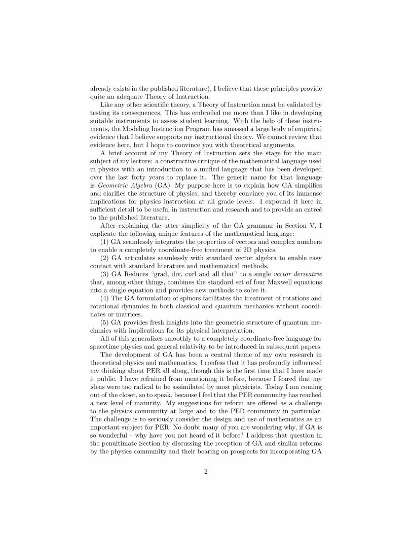
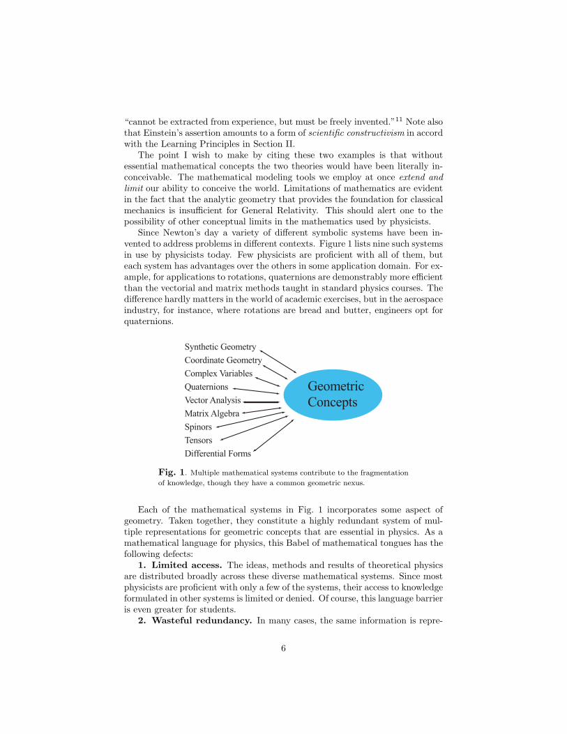
Since Newton’s day a variety of different symbolic systems have been in-vented to address problems in different contexts. Figure 1 lists nine such systemsin use by physicists today. Few physicists are proficient with all of them, buteach system has advantages over the others in some application domain. For ex-ample, for applications to rotations, quaternions are demonstrably more efficientthan the vectorial and matrix methods taught in standard physics courses. Thedifference hardly matters in the world of academic exercises, but in the aerospaceindustry, for instance, where rotations are bread and butter, engineers opt forquaternions.

Fig. 1. Multiple mathematical systems contribute to the fragmentation

of knowledge, though they have a common geometric nexus.

Each of the mathematical systems in Fig. 1 incorporates some aspect ofgeometry. Taken together, they constitute a highly redundant system of mul-tiple representations for geometric concepts that are essential in physics. As amathematical language for physics, this Babel of mathematical tongues has thefollowing defects:

1. Limited access. The ideas, methods and results of theoretical physicsare distributed broadly across these diverse mathematical systems. Since mostphysicists are proficient with only a few of the systems, their access to knowledgeformulated in other systems is limited or denied. Of course, this language barrieris even greater for students.

2. Wasteful redundancy. In many cases, the same information is repre-

6

sented in several different systems, but one of them is invariably better suitedthan the others for a given application. For example, Goldstein’s textbook onmechanics12 gives three different ways to represent rotations: coordinate matri-ces, vectors and Pauli spin matrices. The costs in time and effort for translationbetween these representations are considerable.

3. Deficient integration. The collection of systems in Fig. 1 is not anintegrated mathematical structure. This is especially awkward in problems thatcall for the special features of two or more systems. For, example, vector algebraand matrices are often awkwardly combined in rigid body mechanics, while Paulimatrices are used to express equivalent relations in quantum mechanics.

4. Hidden structure. Relations among physical concepts represented indifferent symbolic systems are difficult to recognize and exploit.

5. Reduced information density. The density of information aboutphysics is reduced by distributing it over several different symbolic systems.

Evidently elimination of these defects will make physics easier to learn andapply. A clue as to how that might be done lies in recognizing that the varioussymbolic systems derive geometric interpretations from a common coherent coreof geometric concepts. This suggests that one can create a unified mathematicallanguage for physics by designing it to provide an optimal representation ofgeometric concepts. In fact, Hermann Grassmann recognized this possibilityand took it a long way more than 150 years ago.13 However, his program tounify mathematics was forgotten and his mathematical ideas were dispersed,though many of them reappeared in the several systems of Fig. 1. A centurylater the program was reborn, with the harvest of a century of mathematicsand physics to enrich it. This has been the central focus of my own scientificresearch.

Creating a unified mathematical language for physics is a problem in thedesign of mathematical systems. Here are some general criteria that I haveapplied to the design of Geometric Algebra as a solution to that problem:

1. Optimal algebraic encoding of the basic geometric concepts: magni-tude, direction, sense (or orientation) and dimension.

2. Coordinate-free methods to formulate and solve basic equations ofphysics.

3. Optimal uniformity of method across classical, quantum and relativis-tic theories to make their common structures as explicit as possible.

4. Smooth articulation with widely used alternative systems (Fig. 1) tofacilitate access and transfer of information.

5. Optimal computational efficiency. The unified system must be atleast as efficient as any alternative system in every application.

Obviously, these design criteria ensure built-in benefits of the unified lan-guage. In implementing the criteria I deliberately sought out the best availablemathematical ideas and conventions. I found that it was frequently necessaryto modify the mathematics to simplify and clarify the physics.

This led me to coin the dictum: Mathematics is too important to beleft to the mathematicians! I use it to flag the following guiding principlefor Modeling Theory: In the development of any scientific theory, a

7

major task for theorists is to construct a mathematical language thatoptimizes expression of the key ideas and consequences of the theory.Although existing mathematics should be consulted in this endeavor, it shouldnot be incorporated without critically evaluating its suitability. I might add thatthe process also works in reverse. Modification of mathematics for the purposesof science serves as a stimulus for further development of mathematics. Thereare many examples of this effect in the history of physics.

Perhaps the most convincing evidence for validity of a new scientific theoryis successful prediction of a surprising new phenomenon. Similarly, the mostimpressive benefits of Geometric Algebra arise from surprising new insights intothe structure of physics.

The following Sections survey the elements of Geometric Algebra and itsapplication to core components of the physics curriculum. Many details andderivations are omitted, as they are available elsewhere. The emphasis is onhighlighting the unique advantages of Geometric Algebra as a unified mathe-matical language for physics.

V. Understanding Vectors

A recent study on the use of vectors by introductory physics students summa-rized the conclusions in two words: “vector avoidance!”14 This state of mindtends to propagate through the physics curriculum. In some 25 years of graduatephysics teaching, I have noted that perhaps a third of the students seem inca-pable of reasoning with vectors as abstract elements of a linear space. Rather,they insist on conceiving a vector as a list of numbers or coordinates. I havecome to regard this concept of vector as a kind of conceptual virus, because itimpedes development of a more general and powerful concept of vector. I callit the coordinate virus! 15

Once the coordinate virus has been identified, it becomes evident that theentire physics curriculum, including most of the textbooks, is infected with thevirus. From my direct experience, I estimate that two thirds of the graduatestudents have serious infections, and half of those are so damaged by the virusthat they will never recover. What can be done to control this scourge? I suggestthat universal inoculation with Geometric Algebra could eventually eliminatethe coordinate virus altogether.

I maintain that the origin of the problem lies not so much in pedagogyas in the mathematics. The fundamental geometric concept of a vector asa directed magnitude is not adequately represented in standard mathematics.The basic definitions of vector addition and scalar multiplication are essentialto the vector concept but not sufficient. To complete the vector concept weneed multiplication rules that enable us to compare directions and magnitudesof different vectors.

8

A. The Geometric Product

I take the standard concept of a real vector space for granted and define thegeometric product ab for vectors a, b, c by the following rules:

(ab)c = a(bc) , associative (1)a(b + c) = ab + ac , left distributive (2)(b + c)a = ba + ca , right distributive (3)

a2 = |a |2 . contraction (4)

where |a | is a positive scalar called the magnitude of a, and |a | = 0 impliesthat a = 0.

All of these rules should be familiar from ordinary scalar algebra. The maindifference is absence of a commutative rule. Consequently, left and right dis-tributive rules must be postulated separately. The contraction rule (4) is pecu-liar to geometric algebra and distinguishes it from all other associative algebras.But even this is familiar from ordinary scalar algebra as the relation of a signednumber to its magnitude.

The rules for multiplying vectors are the basic grammar rules for GA, andthey can be applied to vector spaces of any dimension. The power of GA derivesfrom

• the simplicity of the grammar,• the geometric meaning of multiplication,• the way geometry links the algebra to the physical world.My next task is to elucidate the geometric meaning of vector multiplication.

From the geometric product ab we can define two new products, a symmetricinner product

a ·b = 12 (ab + ba) = b ·a, (5)

and an antisymmetric outer product

a ∧ b = 12 (ab − ba) = −b ∧ a. (6)

Therefore, the geometric product has the canonical decomposition

ab = a ·b + a ∧ b . (7)

From the contraction rule (4) it is easy to prove that a ·b is scalar-valued, soit can be identified with the standard Euclidean inner product. The formallegitimacy and geometric import of adding scalars to bivectors as well as tovectors is discussed in Section VIA.

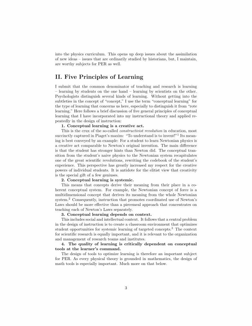
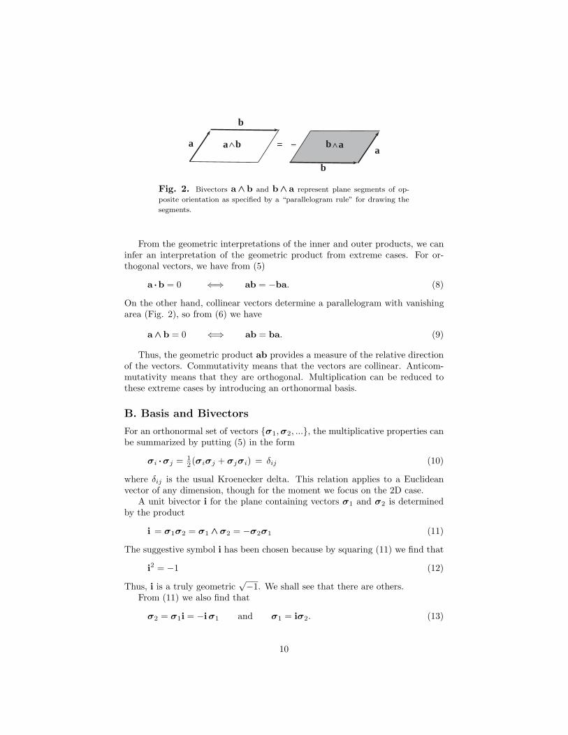
The geometric significance of the outer product a ∧ b should also be familiarfrom the standard vector cross product a × b. The quantity a ∧ b is called abivector, and it can be interpreted geometrically as an oriented plane segment, asshown in Fig. 2. It differs from a × b in being intrinsic to the plane containinga and b, independent of the dimension of any vector space in which the planelies.

9

a

b

a

b

= =a b ab

Fig. 2. Bivectors a ∧ b and b ∧ a represent plane segments of op-

posite orientation as specified by a “parallelogram rule” for drawing the

segments.

From the geometric interpretations of the inner and outer products, we caninfer an interpretation of the geometric product from extreme cases. For or-thogonal vectors, we have from (5)

a ·b = 0 ⇐⇒ ab = −ba. (8)

On the other hand, collinear vectors determine a parallelogram with vanishingarea (Fig. 2), so from (6) we have

a ∧ b = 0 ⇐⇒ ab = ba. (9)

Thus, the geometric product ab provides a measure of the relative directionof the vectors. Commutativity means that the vectors are collinear. Anticom-mutativity means that they are orthogonal. Multiplication can be reduced tothese extreme cases by introducing an orthonormal basis.

B. Basis and Bivectors

For an orthonormal set of vectors σ1,σ2, ..., the multiplicative properties canbe summarized by putting (5) in the form

σi ·σj = 12 (σiσj + σjσi) = δij (10)

where δij is the usual Kroenecker delta. This relation applies to a Euclideanvector of any dimension, though for the moment we focus on the 2D case.

A unit bivector i for the plane containing vectors σ1 and σ2 is determinedby the product

i = σ1σ2 = σ1 ∧ σ2 = −σ2σ1 (11)

The suggestive symbol i has been chosen because by squaring (11) we find that

i2 = −1 (12)

Thus, i is a truly geometric√−1. We shall see that there are others.

From (11) we also find that

σ2 = σ1i = −iσ1 and σ1 = iσ2. (13)

10

In words, multiplication by i rotates the vectors through a right angle. It followsthat i rotates every vector in the plane in the same way. More generally, itfollows that every unit bivector i satisfies (12) and determines a unique plane inEuclidean space. Each i has two complementary geometric interpretations: Itrepresents a unique oriented area for the plane, and, as an operator, it representsan oriented right angle rotation in the plane.

C. Vectors and Complex Numbers

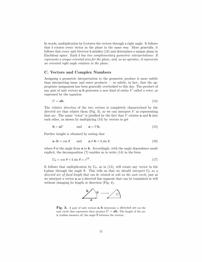
Assigning a geometric interpretation to the geometric product is more subtlethan interpreting inner and outer products — so subtle, in fact, that the ap-propriate assignment has been generally overlooked to this day. The product ofany pair of unit vectors a,b generates a new kind of entity U called a rotor, asexpressed by the equation

U = ab. (14)

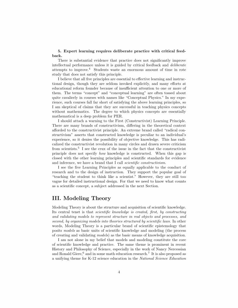
The relative direction of the two vectors is completely characterized by thedirected arc that relates them (Fig. 3), so we can interpret U as representingthat arc. The name “rotor” is justified by the fact that U rotates a and b intoeach other, as shown by multiplying (14) by vectors to get

b = aU and a = Ub . (15)

Further insight is obtained by noting that

a ·b = cos θ and a ∧ b = i sin θ, (16)

where θ is the angle from a to b. Accordingly, with the angle dependence madeexplicit, the decomposition (7) enables us to write (14) in the form

Uθ = cos θ + i sin θ = ei θ . (17)

It follows that multiplication by Uθ, as in (15), will rotate any vector in thei-plane through the angle θ. This tells us that we should interpret Uθ as adirected arc of fixed length that can be rotated at will on the unit circle, just aswe interpret a vector a as a directed line segment that can be translated at willwithout changing its length or direction (Fig. 4).

.b

a. θ

Fig. 3. A pair of unit vectors a,b determine a directed arc on the

unit circle that represents their product U = ab. The length of the arc

is (radian measure of) the angle θ between the vectors.

11

.

a a

a

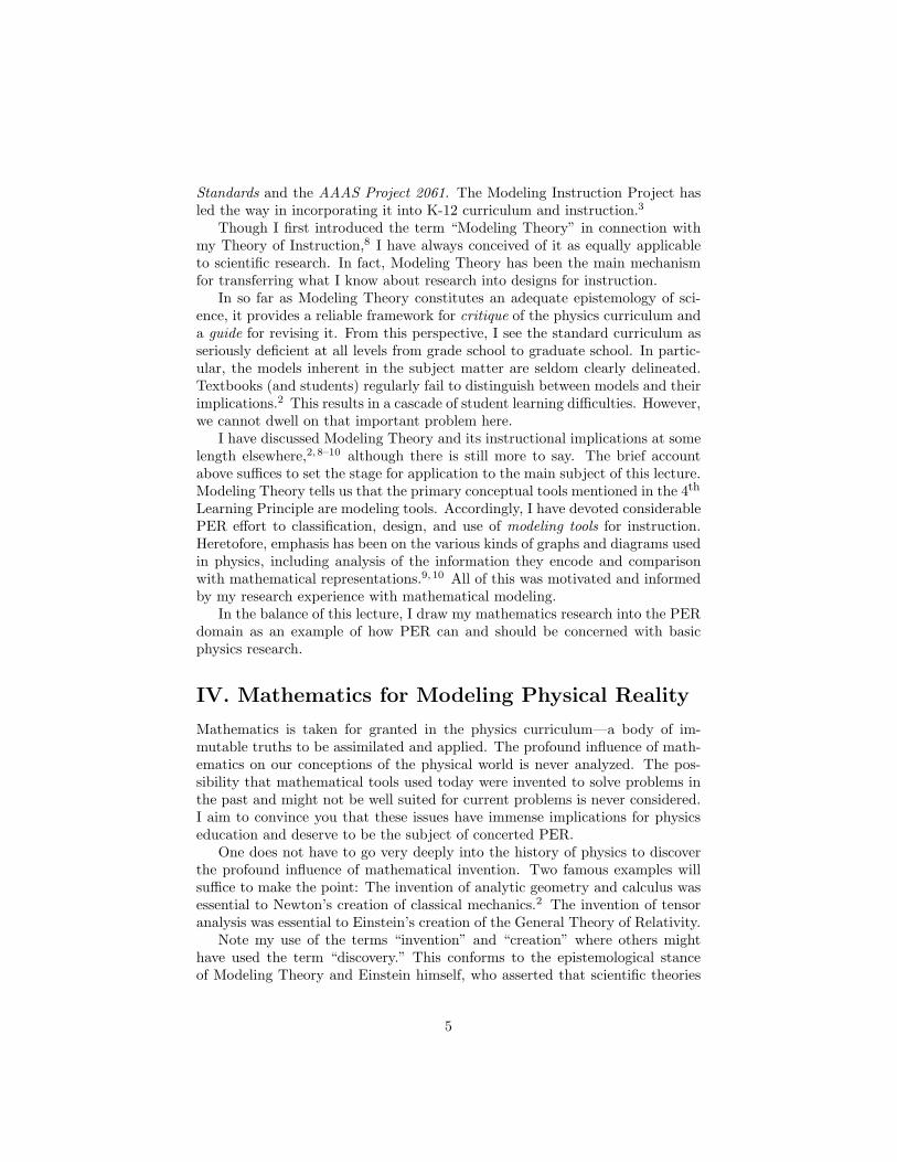
Fig. 4. All directed arcs with equivalent angles are represented by a

single rotor Uθ , just as line segments with the same length and direction

are represented by a single vector a.

ϕϕθ θ +

Fig. 5. The composition of 2D rotations is represented algebraically by

the product of rotors and depicted geometrically by addition of directed

arcs.

With rotors, the composition of 2D rotations is expressed by the rotor prod-uct

UθUϕ = Uθ+ϕ (18)

and depicted geometrically in Fig. 5 as addition of directed arcs.The generalization of all this should be obvious. We can always interpret

the product ab algebraically as a complex number

z = λU = λeiθ = ab, (19)

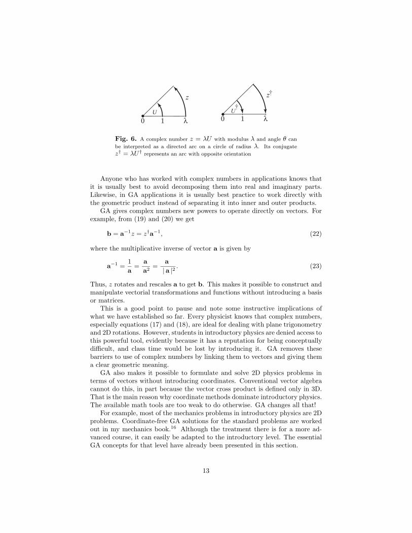
with modulus | z | = λ = |a ||b |. And we can interpret z geometrically as adirected arc on a circle of radius | z | (Fig. 6). It might be surprising that thisgeometric interpretation never appears in standard books on complex variables.Be that as it may, the value of the interpretation is greatly enhanced by its usein geometric algebra.

The connection to vectors via (19) removes a lot of the mystery from complexnumbers and facilitates their application to physics. For example, comparisonof (19) to (7) shows at once that the real and imaginary parts of a complexnumber are equivalent to inner and outer products of vectors. The complexconjugate of (19) is

z† = λU† = λe−i θ = ba, (20)

which shows that it is equivalent to reversing order in the geometric product.This can be used to compute the modulus of z in the usual way:

| z |2 = zz† = λ2 = baab = a2b2 = |a |2|b |2 (21)

12

U.0 1 λ

.0 1 λ

Fig. 6. A complex number z = λU with modulus λ and angle θ can

be interpreted as a directed arc on a circle of radius λ. Its conjugate

z† = λU† represents an arc with opposite orientation

Anyone who has worked with complex numbers in applications knows thatit is usually best to avoid decomposing them into real and imaginary parts.Likewise, in GA applications it is usually best practice to work directly withthe geometric product instead of separating it into inner and outer products.

GA gives complex numbers new powers to operate directly on vectors. Forexample, from (19) and (20) we get

b = a−1z = z†a−1, (22)

where the multiplicative inverse of vector a is given by

a−1 =1a

=aa2

=a|a |2 . (23)

Thus, z rotates and rescales a to get b. This makes it possible to construct andmanipulate vectorial transformations and functions without introducing a basisor matrices.

This is a good point to pause and note some instructive implications ofwhat we have established so far. Every physicist knows that complex numbers,especially equations (17) and (18), are ideal for dealing with plane trigonometryand 2D rotations. However, students in introductory physics are denied access tothis powerful tool, evidently because it has a reputation for being conceptuallydifficult, and class time would be lost by introducing it. GA removes thesebarriers to use of complex numbers by linking them to vectors and giving thema clear geometric meaning.

GA also makes it possible to formulate and solve 2D physics problems interms of vectors without introducing coordinates. Conventional vector algebracannot do this, in part because the vector cross product is defined only in 3D.That is the main reason why coordinate methods dominate introductory physics.The available math tools are too weak to do otherwise. GA changes all that!

For example, most of the mechanics problems in introductory physics are 2Dproblems. Coordinate-free GA solutions for the standard problems are workedout in my mechanics book.16 Although the treatment there is for a more ad-vanced course, it can easily be adapted to the introductory level. The essentialGA concepts for that level have already been presented in this section.

13

Will comprehensive use of GA significantly enhance student learning in in-troductory physics? We have noted theoretical reasons for believing that itwill. To check this out in practice is a job for PER. However, mathematicalreform at the introductory level makes little sense unless it is extended to thewhole physics curriculum. The following sections provide strong justificationfor doing just that. We shall see how simplifications at the introductory levelget amplified to greater simplifications and surprising insights at the advancedlevel.

VI. Classical Physics with Geometric Algebra

This section surveys the fundamentals of GA as a mathematical frameworkfor classical physics and demonstrates some of its unique advantages. Detailedapplications can be found in the references.

A. Geometric Algebra for Physical Space

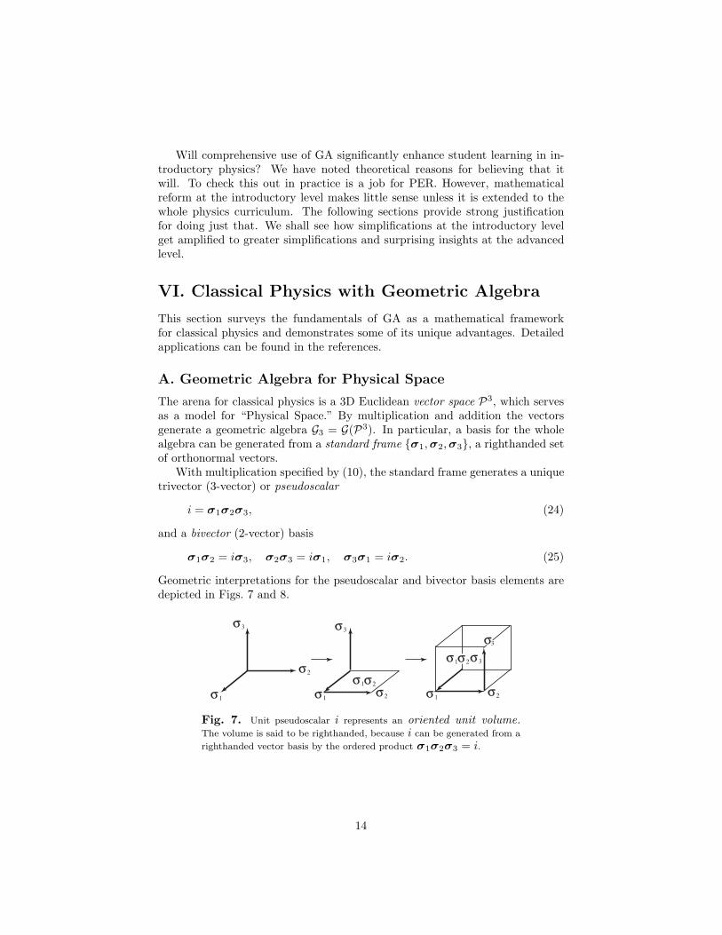
The arena for classical physics is a 3D Euclidean vector space P3, which servesas a model for “Physical Space.” By multiplication and addition the vectorsgenerate a geometric algebra G3 = G(P3). In particular, a basis for the wholealgebra can be generated from a standard frame σ1,σ2,σ3, a righthanded setof orthonormal vectors.

With multiplication specified by (10), the standard frame generates a uniquetrivector (3-vector) or pseudoscalar

i = σ1σ2σ3, (24)

and a bivector (2-vector) basis

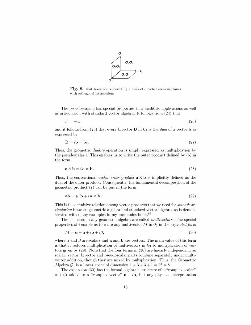
σ1σ2 = iσ3, σ2σ3 = iσ1, σ3σ1 = iσ2. (25)

Geometric interpretations for the pseudoscalar and bivector basis elements aredepicted in Figs. 7 and 8.

σ2

σ1σ2

σ2

σ1σ1

σ2

σ1σ2

σ1

σ3

σ3

σ3σ3

Fig. 7. Unit pseudoscalar i represents an oriented unit volume.The volume is said to be righthanded, because i can be generated from a

righthanded vector basis by the ordered product σ1σ2σ3 = i.

14

σ1

σ1

σ2σ2

σ2σ3σ3σ1

σ3

Fig. 8. Unit bivectors representing a basis of directed areas in planes

with orthogonal intersections

The pseudoscalar i has special properties that facilitate applications as wellas articulation with standard vector algebra. It follows from (24) that

i2 = −1, (26)

and it follows from (25) that every bivector B in G3 is the dual of a vector b asexpressed by

B = ib = bi . (27)

Thus, the geometric duality operation is simply expressed as multiplication bythe pseudoscalar i. This enables us to write the outer product defined by (6) inthe form

a ∧ b = ia × b . (28)

Thus, the conventional vector cross product a × b is implicitly defined as thedual of the outer product. Consequently, the fundamental decomposition of thegeometric product (7) can be put in the form

ab = a ·b + ia × b . (29)

This is the definitive relation among vector products that we need for smooth ar-ticulation between geometric algebra and standard vector algebra, as is demon-strated with many examples in my mechanics book.16

The elements in any geometric algebra are called multivectors. The specialproperties of i enable us to write any multivector M in G3 in the expanded form

M = α + a + ib + iβ, (30)

where α and β are scalars and a and b are vectors. The main value of this formis that it reduces multiplication of multivectors in G3 to multiplication of vec-tors given by (29). Note that the four terms in (30) are linearly independent, soscalar, vector, bivector and pseudoscalar parts combine separately under multi-vector addition, though they are mixed by multiplication. Thus, the GeometricAlgebra G3 is a linear space of dimension 1 + 3 + 3 + 1 = 23 = 8.

The expansion (30) has the formal algebraic structure of a “complex scalar”α + iβ added to a “complex vector” a + ib, but any physical interpretation

15

attributed to this structure hinges on the geometric meaning of i. The mostimportant example is the expression of the electromagnetic field F in terms ofan electric vector field E and a magnetic vector field B:

F = E + iB . (31)

Geometrically, this is a decomposition of F into vector and bivector parts. Instandard vector algebra E is said to be a polar vector while B is an axial vector,the two kinds of vector being distinguished by a difference in sign under spaceinversion. GA reveals that an axial vector is just a bivector represented by itsdual, so the magnetic field in (31) is fully represented by the complete bivectoriB, rather than B alone. Thus GA makes the awkward distinction betweenpolar and axial vectors unnecessary. The vectors E and B in (31) have thesame behavior under space inversion, but an additional sign change comes fromspace inversion of the pseudoscalar.

To facilitate algebraic manipulations, it is convenient to introduce a specialsymbol for the operation (called reversion) of reversing the order of multiplica-tion. The reverse of the geometric product is defined by

(ab)† = ba. (32)

We noted in (20) that this is equivalent to complex conjugation in 2D. From(24) we find that the reverse of the pseudoscalar is

i† = −i. (33)

Hence the reverse of an arbitrary multivector in the expanded form (30) is

M† = α + a − ib − iβ, (34)

The convenience of this operation is illustrated by applying it to the electro-magnetic field F in (31) and using (29) to get

12FF † = 1

2 (E + iB)(E − iB) = 12 (E2 + B2) + E × B, (35)

which is recognized as an expression for the energy and momentum density ofthe field. Note how this differs from the field invariant

F 2 = (E + iB)2 = E2 − B2 + 2i(E·B), (36)

which is useful for classifying EM fields into different types.You have probably noticed that the expanded multivector form (30) violates

one of the basic math strictures that is drilled into our students, namely, that“it is meaningless to add scalars to vectors,” not to mention bivectors andpseudoscalars. On the contrary, GA tells us that such addition is not onlygeometrically meaningful, it is essential to simplify and unify the language ofphysics, as can be seen in many examples that follow.

Shall we say that this stricture against addition of scalars to vectors is amisconception or conceptual virus that infects the entire physics community?

16

At least it is a design flaw in standard vector algebra that has been almostuniversally overlooked. As we have just seen, elimination of the flaw enables usto combine electric and magnetic fields into a single electromagnetic field. Andwe shall see below how it enables us to construct spinors from vectors (contraryto the received wisdom that spinors are more basic than vectors)!

B. Reflections and Rotations

Rotations play an essential role in the conceptual foundations of physics as wellas in many applications, so our mathematics should be designed to handle themas efficiently as possible. We have noted that conventional treatments employan awkward mixture of vector, matrix and spinor or quaternion methods. Mypurpose here is to show how GA provides a unified, coordinate-free treatmentof rotations and reflections that leaves nothing to be desired.

The main result is that any orthogonal transformation U can be expressedin the canonical form16

Ux = ±UxU†, (37)

where U is a unimodular multivector called a versor, and the sign is the parityof U , positive for a rotation or negative for a reflection. The condition

U†U = 1. (38)

defines unimodularity. The underbar notation serves to distinguish the linearoperator U from the versor U that generates it. The great advantage of (37)is that it reduces the study of linear operators to algebraic properties of theirversors. This is best understood from specific examples.

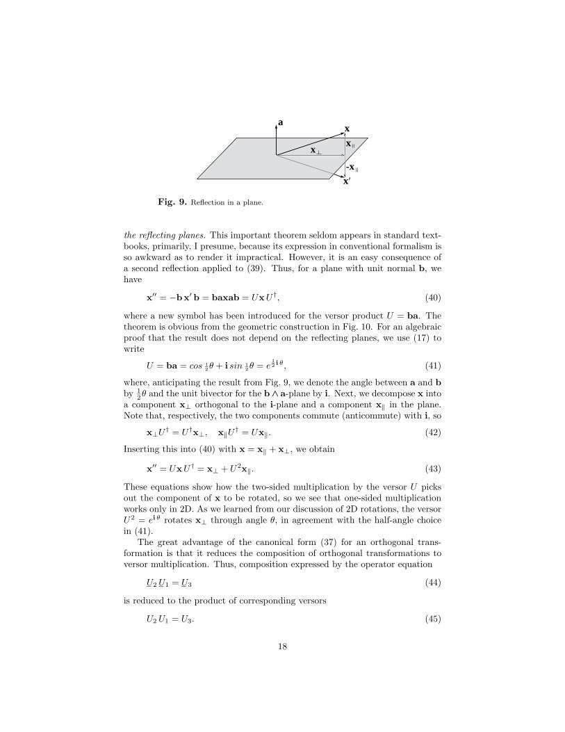
The simplest example is reflection in a plane with unit normal a (Fig. 9),

x′ = −axa = −a(x⊥ + x‖)a = x⊥ − x‖. (39)

To show how this function works, the vector x has been decomposed on theright into a parallel component x‖ = (x ·a)a that commutes with a and anorthogonal component x⊥ = (x ∧ a)a that anticommutes with a. As can beseen below, it is seldom necessary or even advisable to make this decompositionin applications. The essential point is that the normal vector defining the direc-tion of a plane also represents a reflection in the plane when interpreted as aversor. A simpler representation for reflections is inconceivable, so it must bethe optimal representation for reflections in every application, as shown in someimportant applications below. Incidentally, the term versor was coined in the19th century for an operator that can re-verse a direction. Likewise, the term isused here to indicate a geometric operational interpretation for a multivector.

The reflection (39) is not only the simplest example of an orthogonal trans-formation, but all orthogonal transformations can be generated by reflections ofthis kind. The main result is expressed by the following theorem: The productof two reflections is a rotation through twice the angle between the normals of

17

a

xx

x

x-x'

Fig. 9. Reflection in a plane.

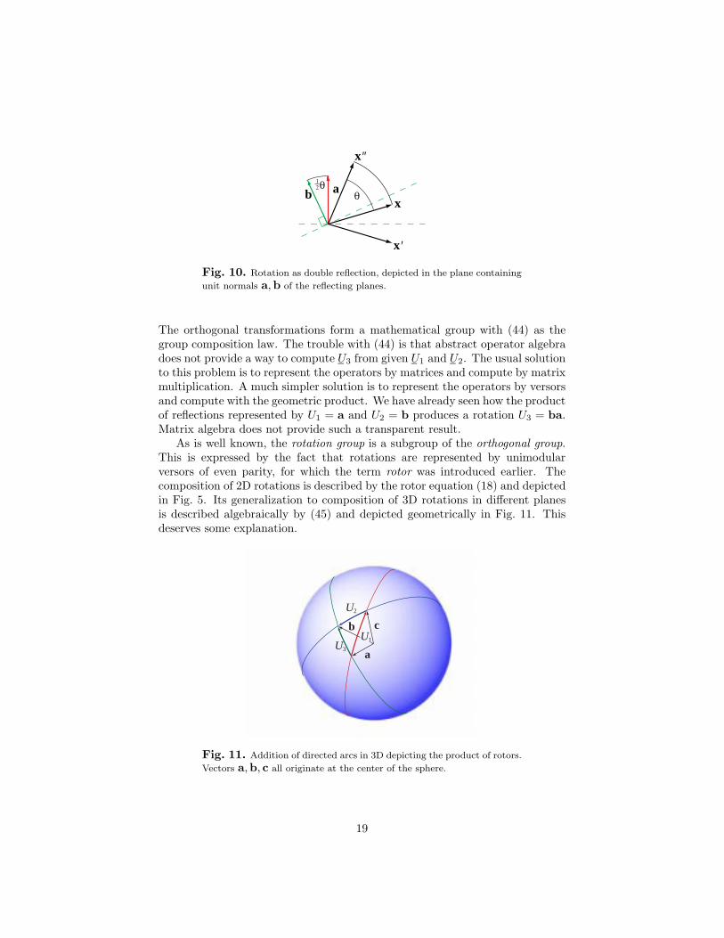
the reflecting planes. This important theorem seldom appears in standard text-books, primarily, I presume, because its expression in conventional formalism isso awkward as to render it impractical. However, it is an easy consequence ofa second reflection applied to (39). Thus, for a plane with unit normal b, wehave

x′′ = −bx′ b = baxab = UxU†, (40)

where a new symbol has been introduced for the versor product U = ba. Thetheorem is obvious from the geometric construction in Fig. 10. For an algebraicproof that the result does not depend on the reflecting planes, we use (17) towrite

U = ba = cos 12θ + i sin 1

2θ = e12 i θ, (41)

where, anticipating the result from Fig. 9, we denote the angle between a and bby 1

2θ and the unit bivector for the b ∧ a-plane by i. Next, we decompose x intoa component x⊥ orthogonal to the i-plane and a component x‖ in the plane.Note that, respectively, the two components commute (anticommute) with i, so

x⊥U† = U†x⊥, x‖U† = Ux‖. (42)

Inserting this into (40) with x = x‖ + x⊥, we obtain

x′′ = UxU† = x⊥ + U2x‖. (43)

These equations show how the two-sided multiplication by the versor U picksout the component of x to be rotated, so we see that one-sided multiplicationworks only in 2D. As we learned from our discussion of 2D rotations, the versorU2 = ei θ rotates x⊥ through angle θ, in agreement with the half-angle choicein (41).

The great advantage of the canonical form (37) for an orthogonal trans-formation is that it reduces the composition of orthogonal transformations toversor multiplication. Thus, composition expressed by the operator equation

U2 U1 = U3 (44)

is reduced to the product of corresponding versors

U2 U1 = U3. (45)

18

abx

x'

x''

θθ1

2

Fig. 10. Rotation as double reflection, depicted in the plane containing

unit normals a,b of the reflecting planes.

The orthogonal transformations form a mathematical group with (44) as thegroup composition law. The trouble with (44) is that abstract operator algebradoes not provide a way to compute U3 from given U1 and U2. The usual solutionto this problem is to represent the operators by matrices and compute by matrixmultiplication. A much simpler solution is to represent the operators by versorsand compute with the geometric product. We have already seen how the productof reflections represented by U1 = a and U2 = b produces a rotation U3 = ba.Matrix algebra does not provide such a transparent result.

As is well known, the rotation group is a subgroup of the orthogonal group.This is expressed by the fact that rotations are represented by unimodularversors of even parity, for which the term rotor was introduced earlier. Thecomposition of 2D rotations is described by the rotor equation (18) and depictedin Fig. 5. Its generalization to composition of 3D rotations in different planesis described algebraically by (45) and depicted geometrically in Fig. 11. Thisdeserves some explanation.

U

a

cb

2

U3

U1

Fig. 11. Addition of directed arcs in 3D depicting the product of rotors.

Vectors a,b, c all originate at the center of the sphere.

19

In 3D a rotor is depicted as a directed arc confined to a great circle on theunit sphere. The product of rotors U1 and U2 is depicted in Fig. 11 by connectingthe corresponding arcs at a point c where the two great circles intersect. Thisdetermines points a = cU1 and b = U2c, so the rotors can be expressed asproducts with a common factor,

U1 = ca, U2 = bc. (46)

Hence (44) gives us

U3 = U2U1 = (bc)(ca) = ba, (47)

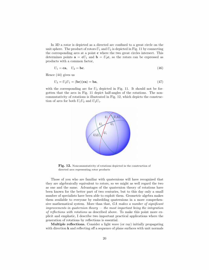
with the corresponding arc for U3 depicted in Fig. 11. It should not be for-gotten that the arcs in Fig. 11 depict half-angles of the rotations. The non-commutativity of rotations is illustrated in Fig. 12, which depicts the construc-tion of arcs for both U1U2 and U2U1.

U2 U2

U1

U1

U1

U2

U2U1

Fig. 12. Noncommutativity of rotations depicted in the construction of

directed arcs representing rotor products

Those of you who are familiar with quaternions will have recognized thatthey are algebraically equivalent to rotors, so we might as well regard the twoas one and the same. Advantages of the quaternion theory of rotations havebeen known for the better part of two centuries, but to this day only a smallnumber of specialists have been able to exploit them. Geometric algebra makesthem available to everyone by embedding quaternions in a more comprehen-sive mathematical system. More than that, GA makes a number of significantimprovements in quaternion theory — the most important being the integrationof reflections with rotations as described above. To make this point more ex-plicit and emphatic, I describe two important practical applications where thegeneration of rotations by reflections is essential.

Multiple reflections. Consider a light wave (or ray) initially propagatingwith direction k and reflecting off a sequence of plane surfaces with unit normals

20

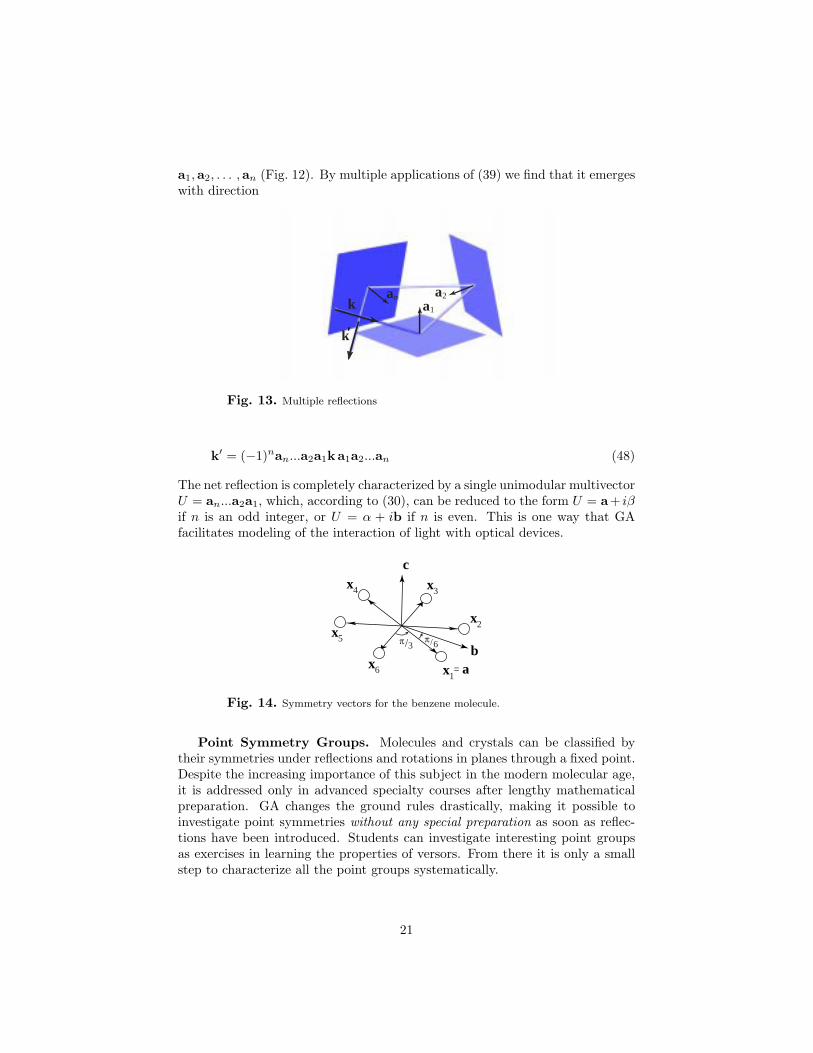
a1,a2, . . . ,an (Fig. 12). By multiple applications of (39) we find that it emergeswith direction

k

k

1ana 2a

'

Fig. 13. Multiple reflections

k′ = (−1)nan...a2a1ka1a2...an (48)

The net reflection is completely characterized by a single unimodular multivectorU = an...a2a1, which, according to (30), can be reduced to the form U = a+ iβif n is an odd integer, or U = α + ib if n is even. This is one way that GAfacilitates modeling of the interaction of light with optical devices.

axb

c

=1

x6

x5

x4

6

x3

3

x2

π π//

Fig. 14. Symmetry vectors for the benzene molecule.

Point Symmetry Groups. Molecules and crystals can be classified bytheir symmetries under reflections and rotations in planes through a fixed point.Despite the increasing importance of this subject in the modern molecular age,it is addressed only in advanced specialty courses after lengthy mathematicalpreparation. GA changes the ground rules drastically, making it possible toinvestigate point symmetries without any special preparation as soon as reflec-tions have been introduced. Students can investigate interesting point groupsas exercises in learning the properties of versors. From there it is only a smallstep to characterize all the point groups systematically.

21

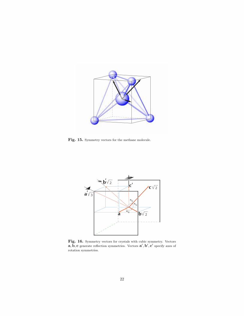
Fig. 15. Symmetry vectors for the methane molecule.

c

π/3

π/2

2

b 2a

c'b 2'

3a'

π/4

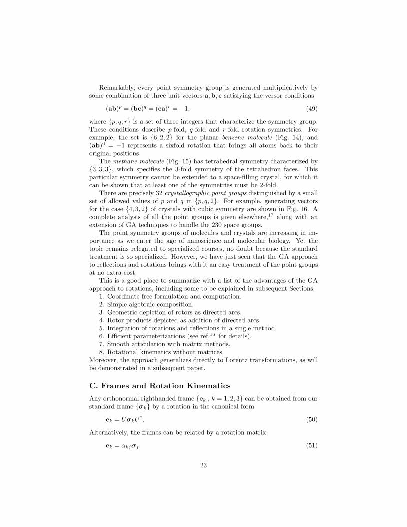
Fig. 16. Symmetry vectors for crystals with cubic symmetry. Vectors

a,b, c generate reflection symmetries. Vectors a′,b′, c′ specify axes of

rotation symmetries.

22

Remarkably, every point symmetry group is generated multiplicatively bysome combination of three unit vectors a,b, c satisfying the versor conditions

(ab)p = (bc)q = (ca)r = −1, (49)

where p, q, r is a set of three integers that characterize the symmetry group.These conditions describe p-fold, q-fold and r-fold rotation symmetries. Forexample, the set is 6, 2, 2 for the planar benzene molecule (Fig. 14), and(ab)6 = −1 represents a sixfold rotation that brings all atoms back to theiroriginal positions.

The methane molecule (Fig. 15) has tetrahedral symmetry characterized by3, 3, 3, which specifies the 3-fold symmetry of the tetrahedron faces. Thisparticular symmetry cannot be extended to a space-filling crystal, for which itcan be shown that at least one of the symmetries must be 2-fold.

There are precisely 32 crystallographic point groups distinguished by a smallset of allowed values of p and q in p, q, 2. For example, generating vectorsfor the case 4, 3, 2 of crystals with cubic symmetry are shown in Fig. 16. Acomplete analysis of all the point groups is given elsewhere,17 along with anextension of GA techniques to handle the 230 space groups.

The point symmetry groups of molecules and crystals are increasing in im-portance as we enter the age of nanoscience and molecular biology. Yet thetopic remains relegated to specialized courses, no doubt because the standardtreatment is so specialized. However, we have just seen that the GA approachto reflections and rotations brings with it an easy treatment of the point groupsat no extra cost.

This is a good place to summarize with a list of the advantages of the GAapproach to rotations, including some to be explained in subsequent Sections:

1. Coordinate-free formulation and computation.2. Simple algebraic composition.3. Geometric depiction of rotors as directed arcs.4. Rotor products depicted as addition of directed arcs.5. Integration of rotations and reflections in a single method.6. Efficient parameterizations (see ref.16 for details).7. Smooth articulation with matrix methods.8. Rotational kinematics without matrices.

Moreover, the approach generalizes directly to Lorentz transformations, as willbe demonstrated in a subsequent paper.

C. Frames and Rotation Kinematics

Any orthonormal righthanded frame ek , k = 1, 2, 3 can be obtained from ourstandard frame σk by a rotation in the canonical form

ek = UσkU†. (50)

Alternatively, the frames can be related by a rotation matrix

ek = αkjσj . (51)

23

These two sets of equations can be solved for the matrix elements as a functionof U , with the result

αkj = ek ·σj = 〈UσkU†σj〉, (52)

where 〈...〉 means scalar part. Alternatively, they can be solved for the rotor asa function of the frames or the matrix.16 One simply forms the quaternion

ψ = 1 + ekσk = 1 + αkjσjσk (53)

and normalizes to get

U =ψ

(ψψ†)12. (54)

This makes it easy to move back and forth between matrix and rotor representa-tions of a rotation. We have already seen that the rotor is much to be preferredfor both algebraic computation and geometric interpretation.

Let the frame ek represent a set of directions fixed in a rigid body, perhapsaligned with the principal axes of the inertia tensor. For a moving body the ek =ek(t) are functions of time, and (50) reduces the description of the rotationalmotion to a time dependent rotor U = U(t). By differentiating the constraintUU† = 1, it is easy to show that the derivative of U can be put in the form

dU

dt= 1

2ΩU, (55)

where

Ω = −iω (56)

is the rotational (angular) velocity bivector. By differentiating (50) and using(55), (56), we derive the familiar equations

dek

dt= ω × ek (57)

employed in the standard vectorial treatment of rigid body kinematics.The point of all this is that GA reduces the set of three vectorial equations

(57) to the single rotor equation (55), which is easier to solve and analyze forgiven Ω = Ω(t). Specific solutions for problems in rigid body mechanics arediscussed elsewhere.16 However, the main reason for introducing the classicalrotor equation of motion in this lecture is to show its equivalence to equationsin quantum mechanics given below.

24

D. Maxwell’s Equation

We have seen how electric and magnetic field vectors can be combined into asingle multivector field

F (x, t) = E(x, t) + iB(x, t) (58)

representing the complete electromagnetic field. Standard vector algebra forcesone to consider electric and magnetic parts separately, and it requires four fieldequations to describe their coordinated action. GA enables us to put HumptyDumpty together and describe the complete electromagnetic field by a singleequation. But first we need to learn how to differentiate with respect to theposition vector x.

We can define the derivative ∇ = ∂x with respect to the vector x mostquickly by appealing to your familiarity with the standard concepts of divergenceand curl. Then, since ∇ must be a vector operator, we can use (29) to definethe vector derivative by

∇E = ∇·E + i∇ × E = ∇·E + ∇ ∧ E . (59)

This shows the divergence and curl as components of a single vector derivative.Both components are needed to determine the field. For example, for the fielddue to a static charge density ρ = ρ(x), the field equation is

∇E = ρ. (60)

The advantage of this form over the usual separate equations for divergence andcurl is that ∇ can be inverted to solve for

E = ∇−1ρ. (61)

Of course ∇−1 is an integral operator determined by a Green’s function, but GAprovides new insight into such operators. For example, for a source ρ with 2Dsymmetry in a localized 2D region R with boundary ∂R, the E field is planarand ∇−1 can be given the explicit form18,19

E(x) =12π

∫R

| d2x′ | 1x′ − x

ρ(x′) +1

2πi

∮∂R

1x′ − x

dx′E(x′), (62)

where i is the unit bivector for the plane. In the absence of sources, the firstintegral on the right vanishes and the field within R is given entirely by a lineintegral of its value over the boundary. The resulting equation is precisely equiv-alent to the celebrated Cauchy integral formula, as is easily shown by changingto the complex variable z = xa, where a is a fixed unit vector in the plane thatdefines the “real axis” for z. Thus GA automatically incorporates the full powerof complex variable theory into electromagnetic theory. Indeed, formula (62)generalizes the Cauchy integral to include sources and the generalization can beextended to 3D with arbitrary sources.18,19 But this is not the place to discusssuch matters.

25

An electromagnetic field F = F (x, t) with charge density ρ = ρ(x, t) andcharge current J = J(x, t) as sources is determined by Maxwell’s Equation

( 1c

∂t + ∇ )F = ρ − 1

cJ . (63)

To show that this is equivalent to the standard set of four equations, we employ(58), (59) and (30) to separate, respectively, its scalar, vector, bivector, andpseudoscalar parts:

∇·E = ρ, (64)

1c

∂tE − ∇ × B = −1cJ, (65)

i1c

∂tB + ∇ × E = 0, (66)

i∇·B = 0 (67)

Here we see the standard set of Maxwell’s equations as four geometrically dis-tinct parts of one equation. Note that this separation into several parts is similarto separately equating real and imaginary parts in an equation for complex vari-ables.

Of course, it is preferable to solve and analyze Maxwell’s Equation withoutdecomposing it into parts. This is especially true for propagating wave solutions.For example, monochromatic plane waves in a vacuum have solutions with thefamiliar form

F (x, t) = fe±i(ωt−k·x). (68)

What may not be so familiar to physicists is that

F 2 = f2 = 0 (69)

is required here, the i is the unit pseudoscalar and the two signs in (68) representthe two states of circular polarization. A more detailed GA treatment of planewaves was published in this journal three decades ago.20

VII. Real Quantum Mechanics

Schroedinger’s version of quantum mechanics requires that the state of an elec-tron be represented by a complex wave function ψ = ψ(x, t), and Born addedthat the real bilinear function

ρ = ψψ† (70)

should be interpreted as a probability density for finding the electron at pointx at time t. This mysterious relation between probability and a complex wave

26

function has stimulated a veritable orgy of philosophical speculation about thenature of matter and our knowledge of it. Curiously, virtually all philosophizingabout the interpretation of quantum mechanics has been based on Schroedingertheory, despite the fact that electrons, like all other fermions, are known tohave intrinsic spin. We shall see that that is a serious mistake, for it is only ina theory with electron spin that one can see why the wave function is complex.You may wonder why this fact is not common knowledge.

The reason is that the geometric meaning of the wave function lies buriedin the standard matrix version of the Pauli theory. We shall exhume it bytranslating the matrix wave function Ψ into a real spinor ψ in GA where, aswe have seen, every

√−1 has a geometric meaning. We discover then that the√−1 in Schroedinger theory emerges in the real Pauli version as a bivector thatis related to spin in an essential way. In other words, we see that geometrydictates that spin is not a mere add-on in quantum mechanics, but an essentialfeature of fermion wave functions.

By reformulating quantum mechanics in terms of real spinors, we establishGA as a common mathematical language for quantum mechanics and classicalmechanics as formulated in preceding Sections. This simplifies and clarifies therelation of classical theory to quantum theory. In particular, we find that thespinor wave function operates as a rotor in essentially the same way as rotors inclassical mechanics. This suggests that the bilinear dependence of observableson the wave function is not unique to quantum mechanics — it is equally naturalin classical mechanics for geometrical reasons.

Though the relation of spin to the unit imaginary was first discovered in theDirac theory,21,22 it is easiest to see in the Pauli theory. The resulting real spinorwave equation leads to the surprising conclusion that spin was inadvertentlyincorporated into the original Schroedinger equation in the guise of the distinctivefactor

√−1h. Extension to the Dirac theory will be covered in a sequel to thispaper.

A. Vectors vs. Matrices

No doubt some of you noticed in Section VB the similarity of the basis vectors σi

to the Pauli spin matrices. Indeed, the Pauli algebra is a matrix representationof the geometric algebra G3. I have co-opted the standard symbols σi for Paulimatrices to make the correspondence as obvious as possible. To emphasize thatcorrespondence, I use the same symbols σi for the basis vectors and the Paulimatrices that represent them.

My purpose is to lay bare some serious misconceptions that complicate quan-tum mechanics and obscure its relation to classical mechanics. The most basic ofthese misconceptions is that the Pauli matrices are intrinsically related to spin.On the contrary, I claim that their physical significance is derived solely fromtheir correspondence with orthogonal directions in space. The representation ofσi by 2×2 matrices is irrelevant to physics. That being so, it should be possibleto eliminate matrices altogether and make the geometric structure of quantummechanics explicit through direct formulation in terms of GA. How to do that

27

is explained below. For the moment, we note the potential for this change inperspective to bring classical mechanics and quantum mechanics closer together.

Texts on quantum mechanics describe the three σi as a vector σ with ma-trices for components. They combine σ with an ordinary vector a with scalarcomponents ai by writing

σ ·a = aiσi. (71)

(sum over repeated indices). Then they derive the identity

σ ·a σ ·b = a ·b I + iσ · (a × b). (72)

where I is the identity matrix. This formula relating vector algebra to Paulialgebra is a prime example of wasteful redundancy in standard physics, for weknow that the two algebras have common geometric content. GA eliminatesthis redundancy entirely. Indeed, (72) is the matrix representation of the GAproduct formula (29), where it is seen not as a relation between different algebrasbut between different geometric products.

B. Pauli’s Matrix Theory

To set the stage for deriving the GA version of nonrelativistic quantum me-chanics, a brief review of Pauli’s matrix theory is in order. To describe anelectron with spin, Pauli generalized Schroedinger’s complex wave function toa column matrix Ψ with two complex components representing “spin up” and“spin down” states. The two spin states with Ψ± are eigenstates of a hermitianspin operator

σ3Ψ± = ±Ψ±. (73)

A complete set of hermitian spin operators is given by the Pauli matrices

σ1 =(

0 11 0

), σ2 =

(0 −i′

i′ 0

), σ3 =

(1 00 −1

), (74)

where i′ =√−1 is a scalar imaginary with no geometric significance, so (as we

shall see) no physical significance!To describe the interaction of electron spin with an external magnetic field

B, Pauli added an interaction term to Schroedinger’s equation for his two com-ponent wave function, with the result

i′h ∂tΨ = HS Ψ − eh

2mcσ ·BΨ (75)

where HS is the Schroedinger hamiltonian and σ ·B is as defined in (71). Pauliinserted the coefficient of the interaction term “by hand,” assuming a gyromag-netic ratio g = 2 to agree with experiment. When Dirac derived it shortlythereafter, the result was regarded as confirmation of the Dirac equation and aconsequence of relativity theory. However, it was realized much later that the

28

coefficient can be derived by mimicking Dirac’s argument in the nonrelativisticdomain, so spin is not a “relativistic phenomenon” after all. The trick is todefine a momentum operator

σ · p = σ · (−i′h∇ − e

cA) (76)

and assume a hamiltonian of the form

HP =1

2m(σ · p )2 + V (x) . (77)

When this is expanded with the help of the identity (72), it gives the resultin (75). I do not know who originated this argument, but I learned it fromFeynman, who gave me the impression that he had devised it himself. As wesee below, the definition (76) of the momentum operator is less mysterious inGA, where it is apparent that the appearance of σ in it has nothing to do withspin. Indeed, the “trick” (76) is justified by GA, where σi appear naturally asbasis for the vector A and the vector derivative ∇.

C. Real Pauli-Schroedinger Theory

This section proves that the Pauli wave function can be represented as a realspinor (or quaternion) satisfying a real wave equation in the geometric algebraG3 = G(P3) introduced in Section VI for classical physics. The resulting realversion of Pauli-Schroedinger electron theory is isomorphic to the standard ma-trix version, but it has a more transparent geometric structure that elucidatesand simplifies physical interpretation and relations to classical mechanics. Theobjective here is to develop the “real theory” to the point where it is ready tobe used in applications with no further appeal to the matrix theory, except tomake contact with the literature.

We can extract the “real” version of the Pauli theory from the matrix versionin the following way.23 Consistent with the representation of Pauli matrices (74),let u be a basis spinor for the “spin-up” eigenstate of σ3, so we can write

σ3u = u, where u =(

10

). (78)

Then(74) gives us

σ1σ2u = i′u. (79)

Now write Ψ in the form

Ψ = ψu, (80)

where ψ is a polynomial in the Pauli matrices. The coefficients in this polynomialcan be taken as real, for if there is a term with an imaginary coefficient, we canuse (79) to replace i′ by multiplication with σ1σ2 on the right side of the term.

29

Furthermore, the polynomial can be taken as an even multivector, for if anyterm is odd, then (78) allows us to make it even by multiplying it on the rightby σ3. Therefore, we can assume with complete generality that ψ in (80) is areal even multivector. Now we can reinterpret the σk in ψ as vectors in GAinstead of matrices. Thus, we have established a one-to-one correspondencebetween Pauli spinors Ψ and even multivectors ψ in GA.

Since the ungeometrical imaginary i′ has been thereby eliminated, I refer toψ as a real spinor (or quaternion). Note that ψ has four degrees of freedom, onefor its scalar part and three for its bivector part, as does Ψ in its two complexmatrix components. The big gain in replacing Ψ by ψ is that the latter has amore transparent geometric interpretation, as shown below.

Now, it is easy to extract a real wave equation for the real spinor wavefunction from the matrix equation (75). Thus we arrive at the real Pauli-Schroedinger (PS) equation

∂t ψ iσ3h = HS ψ − eh

2mcBψσ3, (81)

where i is now the unit pseudoscalar so iσ3 = σ1σ2, and σ ·B is replaced byB for reasons explained above. I have inserted Schroedinger’s name here toemphasize the fact (explained below) that in this real theory the Schroedingerwave function is the same real spinor, and (81) reduces to the Schroedingerequation by dropping the last term. In the same way, equations (76) and (77)can be re-expressed in the real theory, but we will not have need of them below.

The equivalence of (81) to the matrix equation (75) is easily proved byinterpreting (81) as a matrix equation, multiplying on the right by the basisspinor u and using (78), (79) and (80). Note that the σ3 on the right side of(81) is essential to make the last term have even parity, for the vector B is oddwhile ψ is an even multivector. Thus all terms in (81) are even.

It should be noted that the condition imposed in the Pauli theory by as-suming that the Pauli spin matrices are hermitian is equivalent to the definition(34) of reversion in GA. Thus we see that the standard association of “spinobservables” with hermitian operators amounts to declaring that they representvectors. Evidently, this is an assumption about geometry rather than spin —a critical geometric assumption that has been inadvertently incorporated intoquantum mechanics. Spin must get into the theory some other way. This raisesserious questions about the physical significance of the common association ofphysical observables with hermitian operators.

The explicit σ3 in equation (81) may make it look less general than (75),but that is an illusion, because σ3 is an arbitrarily chosen constant vector. Itcan be related to any other choice σ′

3 by a constant rotation

σ′3 = CσkC†, (82)

Thus, multiplication of (81) on the right by C† gives

(ψσ3)C† = ψC†Cσ3C† = ψ′σ′

3, (83)

30

where ψ′ = ψC† is the wave function relative to the alternative quantizationaxis σ′

3. The matrix analog of this transformation is a change in matrix repre-sentation for the column spinor Ψ.

D. Interpretation of the Real Wave Function.

Having established equivalence to the standard matrix theory, from now on wecan work with the real theory alone. Our main objective is to establish thephysical meaning of the real wave function ψ = ψ(x, t). Adopting the Bornprobability assumption (70), we can write

ψ = ρ12 U, where UU† = 1. (84)

This determines a frame of bilinear “local observables”

ψσkψ† = ρ ek, (85)

where σk is a standard frame and, of course,

ek = UσkU†. (86)

These observables are invariant under the change in choice of standard frameψσkψ† = ψ′σ′

kψ′† defined by (82). Thus, the wave function determines aninvariant time-dependent field of frames ek(x, t) attached to each position x.We show below that

s = 12 h e3 = 1

2 h Uσ3U† (87)

can be interpreted as a spin vector, so ρ s is a spin density. Actually, angularmomentum is a bivector quantity, so it is more correct to represent spin by thebivector

S = i s =h

2U iU† =

h

2e1e2, (88)

where

i ≡ iσ3 = σ1σ2 (89)

plays the role of√−1 in the real PS equation (81).

The hidden relation of spin to the imaginary i′ in the matrix theory can bemade more manifest by regarding S = Sijσjσi as a spin operator on the wavefunction. Multiplying (88) on the right by (84) we get

Sψ = ψih

2. (90)

Regarding this as a matrix equation, we use (80) and (79) to get

SΨ = 12 i′h Ψ. (91)

31

Thus, 12 i′h is the eigenvalue of the “spin operator” S. Otherwise said, the factor

i′h in the Pauli matrix equation (75) is a representation of the spin bivector byits eigenvalue. The eigenvalue is imaginary because the spin tensor Sij = −Sji

is skewsymmetric. We can conclude, therefore, that spin was originally intro-duced into quantum mechanics with the factor i′h in the original Schroedingerequation.

Spin components sk = s ·σ3 = 〈sσ3〉 are related to conventional matrixelements by

ρsk =h

2〈σkψσ3ψ

†〉 =h

2Tr (σkΨΨ†) =

h

2Ψ†σkΨ, (92)

where the scalar part 〈M〉 of a real multivector M corresponds to the TraceTr (M) of its matrix representation.

In conventional Pauli theory,31 the σk are regarded as “spin operators” witheigenvalues corresponding to results of spin measurements in orthogonal direc-tions. However, (92) shows that in Real PS Theory the σk are operators onlyin the trivial sense of basis vectors that pick out components of the spin vectordetermined by the wave function. Conventional theory also interprets the non-vanishing commutator [σ1,σ2] = σ1σ2 −σ2σ1 as a measure of incompatibilityin spin measurements. Whereas, according to (11) and (25), the real theoryinterprets

[σ1,σ2] = 2σ1 ∧ σ2 = 2iσ3 (93)

as a geometric product with no particular relation to spin. This raises seriousquestions about the conventional view of spin in quantum mechanics. Morequestions are raised by further study of the real theory.24

The role of spin in the PS equation (81) can be made explicit by using (87)to write the last term in the form

− eh

2mcBψσ3 = 1

2

( e

mciB

)ψih = − e

mcBsψ. (94)

Note that

Bs = B · s + i(B × s) (95)

splits into terms proportional to magnetic energy and torque.A physical interpretation of the PS equation is supplied by Schroedinger’s

assumption that the energy E of a stationary state is given by the eigenvalueequation

∂t ψ ih = Eψ. (96)

Pauli’s additional term changes this to

E = ES − e

mcB · s, (97)

32

where ES is the Schroedinger energy. For a stationary solution with B × s = 0,s must be parallel or antiparallel to B and we have

B · s = ± h

2|B |. (98)

This is the basis for declaring that spin is “two-valued.” However, when B isvariable the vectorial nature of s becomes apparent.

We can generalize (96) to arbitrary states by interpreting

ρE = 〈∂t ψ iσ3hψ†〉. (99)

as energy density. Here the energy E = E(x, t) can be a variable function, andwe see that an energy eigenstate is defined by the assumption that E is uniform.Inserting (84) into (99), we discover that the density ρ drops out to give us

E = 〈∂t U iσ3hU†〉. (100)

To interpret this expression we need to relate it to observables, in particular,the spin.

As we have seen before, the unimodularity condition on U implies that itsderivative can be written in the form

∂t U = −12 iωU, (101)

so that (86) gives us

∂t ek = ω × ek, (102)

in exact correspondence with the classical equations (55) and (57). In particular,(102) gives us the kinematic equation for spin precession

∂t s = ω × s. (103)

Inserting (101) into (100) and using (87) we get

E = ω · s =12ω ·2s. (104)

This is identical to the classical expression for the rotational kinetic energy ofa rigid body with angular momentum 2s.16 All this suggests that the rotor Udescribes continuous kinematics of electron motion rather than a probabilisticcombination of spin-up and spin-down states as asserted in conventional Paulitheory.

The most surprising thing about the energy expression (104) is that it appliesto any solution of the Schroedinger equation, where ω × s = 0. But, accordingto (102), e1 and e2 are spinning about the spin axis with angular velocity ω,and (104) associates energy with the rotation rate. The big question is, “What isthe physical meaning of this spinning?” I have discussed one intriguing answer

33

at some length before,24 and I will return to it in a subsequent paper within thecontext of the Dirac theory.

When the magnetic field B = B(t) is a function of time alone, we can definea rotor D by assuming that it satisfies the equation

dD

dt= 1

2

( e

mciB

)D. (105)

and factoring the wave function into

ψ = ψ(x, t) = D(t)ψS(x, t). (106)

Substituting this into the PS-equation (81) separates the factors so that Dsatisfies (105) and ψS satisfies Schroedinger’s equation

∂t ψS ih = HS ψS . (107)

The rotor equation (105) exhibits a magnetic torque (e/m)B in perfect agree-ment with the classical model of magnetic resonance discussed in my book.16

This exact analogy with classical physics is a great help in interpreting magneticresonance experiments, and it raises more questions about the interpretation ofelectron spin.

Note that the factor 12 on the right side of (105) is the same factor that,

following Pauli, was attributed to spin in (87) and (98). However, (105) and(101) suggest that the 1

2 is more correctly associated with the rotational velocityin a rotor equation.

Although our real version of the Pauli theory gives new insight into thegeometric properties of the wave function, spin and interaction with the mag-netic field, it is mathematically isomorphic with the standard matrix version,so no new physical consequences are to be expected, and it is straightforwardto translate results from one version to the other. More details about the realPS theory have been published in this journal before.24

Standard techniques for analyzing angular momentum and solving the Pauliequation31 can be converted to GA,25 where they yield some surprises andsimplifications that deserve further study.

Without delving into the complexities of angular momentum analysis, it isobvious that the standard Schroedinger wave function is a solution the Schroe-dinger equation (107), but with the bivector i = iσ3 as unit imaginary, so thereis no way to eliminate spin from the theory without eliminating complex num-bers. It must be concluded, therefore, that standard Schroedinger theory doesnot describe electrons without spin, but rather electrons with constant spin (or,equivalently, electrons in a spin eigenstate).

The difference between Pauli and Schroedinger solutions of (107) is in theclass of eigenfunctions allowed. The simple Schroedinger hamiltonian HS doesnot discriminate between them. A distinction is forced when the hamiltonian isgeneralized to include spin-orbit interactions,31 but this is not the place to gointo details.

34

This discussion has been limited to single particle Pauli theory. But inclosing, it should be mentioned that GA methods for spin representations ofmany particle systems is currently an area of active research,32,38 where GAgives fresh insights into entangled states, quantum computing and the like.

To summarize, let me highlight the most provocative conclusions from thissection:

• The explicit√−1 in fermion wave functions represents a bivector specifying

the direction of spin.

• ih = iσ3h represents spin in Schroedinger’s equation. This implies thatspin is not a simple add-on in quantum mechanics but an essential ingredientof the theory. That is likely to be true for all fermions and bosons that arecomposites of fermions.

• Pauli matrices represent vectors, not spin operators in quantum mechanics.

• Bilinear observables are geometric consequences of rotational kinematics,so they are as natural in classical mechanics as in quantum mechanics.

• The real spinor wave function is easier to interpret and solve than thematrix version.

VIII. Prospects for Curriculum Reform

Our physics curriculum has been largely shaped by the efforts of “lone wolf”textbook writers, and we owe them a debt of gratitude for their fine contribu-tions. Nevertheless, the curriculum would be well served by scholarly critiqueand analysis to identify weaknesses and promote constructive innovation. I sub-mit that this is worthy activity for the PER community. A community is neededto incubate innovations and promote them when they are ready for wide adop-tion. The prevailing laissez-faire process of textbook adoption has suppressedmany fine contributions. It also fails to address problems of integration andcoherence of the whole curriculum, as textbook reform tends to be confined to asingle course. As a case in point, I submit the problem of integrating geometricalgebra into the physics curriculum.

Assuming, for the sake of argument, that there is strong support for GA inthe physics community, what will it take to integrate it into the curriculum?History tells us that it will take a long time if left to normal evolutionary pro-cesses. In a perceptive essay on “fashionable pursuits” in science,28 FreemanDyson argues that innovations in mathematical physics are almost always un-fashionable when they are introduced, and he estimates that it takes fifty toa hundred years for them to achieve general recognition. It is clear that newmechanisms for curriculum reform will be needed to accelerate adoption of GA,or any other substantial reform for that matter. As an indicator of difficultiesinvolved and prospects for success, I offer a brief account of my own experiencewith GA and discuss some hurdles to broad adoption.

35

A. History and reception of geometric algebra

Geometric algebra originated in the work of Hermann Grassmann (1809–1877)and William Kingdon Clifford (1845–1879). Clifford provided the axiomaticformulation for the geometric product in Section VA, so the system is calledClifford algebra in most of the mathematics literature. However, Clifford him-self called it geometric algebra, and he acknowledged the primary contributionof Grassmann. He recognized its unique significance as an algebraic represen-tation of geometric concepts as conceived by Grassmann. Unfortunately, hisdeep insight into the geometric foundations of algebra did not survive his earlydeath. Mathematicians abstracted Clifford algebra from its geometric origins,and, for the better part of a century, it languished as a minor subdiscipline ofmathematics — one more algebra among so many others.

Grassmann’s program to develop a universal geometric algebra for mathe-matics and physics was revived in 1966 with my book Space Time Algebra.21

Actually, it was many years later before I realized how much of my own researchprogram for developing a universal mathematical language had been anticipatedby Grassmann.13 Of course, I had an additional century of mathematics andphysics to draw on, so geometric algebra today is vastly more developed with ascope that was inconceivable in Grassmann’s day.

My 1966 book introduced the critical innovations that made the unifiedlanguage in this paper possible. It developed a coordinate-free formulation ofspacetime physics that will be discussed in the sequel to this paper. Afteremploying it exclusively in my research and teaching over the next few years,my own perspective on GA in physics was consolidated around the essentialform and content in this lecture. I found GA so empowering that ever since Ihave not been satisfied with my understanding of any subject in physics until Ihave formulated it in terms of GA. Invariably I have found that GA simplifiesand illuminates every subject.

My 1966 book had a serious limitation. Though it simplified the funda-mental equations of physics, applications required access to the great repertoireof available mathematical methods, and translation into standard formulationsoften destroyed the advantages of geometric algebra. This motivated me toextend geometric algebra to a unified language for mathematics that incorpo-rated all the methods needed in physics. Besides, I must confess to an abidinginterest in pure mathematics for its own sake. I consider myself equal partsmathematician and physicist. This ambitious program to redesign mathematicswas greatly stimulated by an amazing early success: the realization that GAenables a natural generalization and extension to arbitrary dimension of thecentral result of complex variable theory, Cauchy’s integral formula.18 This re-sult has been independently discovered by several others, and mathematicianshave developed it in recent years into a vigorous new branch of mathematicscalled Clifford analysis. Unfortunately, most practitioners in this field pay insuf-ficient attention to the geometric meaning of their results that is needed for easyapplication to physics. Consequently, the evolution of geometric algebra into acomprehensive Geometric Calculus to serve as a unified language for both math-

36

ematics and physics has so far proceeded independently of Clifford analysis.29

The development of Geometric Calculus culminated in the 1986 publication ofa comprehensive mathematics monograph19 and has continued to this day. Tomy knowledge, no other mathematical system integrates such a broad range ofmathematics, just about all the mathematics needed for physics.

For the first 20 years of my professional life my research on developing andapplying geometric algebra proceeded in almost complete isolation, except forinteraction with a few students. During that period I published regularly, butthere were only a handful of citations to my papers and no positive feedback fromcolleagues. I learned to be very careful about when, where and how I presentedmy work to other physicists, because the reaction was invariably dismissive assoon as they detected deviation from standard practice or beliefs.27

I did not even try to publish in Physical Review. Instead, I conducteda sociological experiment by submitting proposals to the NSF for support ofmy work on relativistic electron theory. After the first couple of tries I wasconvinced that it would never get funded, but I continued to submit 12 times inall as an experiment on how the system works. I found that there was alwaysa split opinion on my proposal that typically fell into three groups. Aboutone third dismissed me outright as a crank. About one third was intriguedand sometimes gave my proposal an Excellent rating. The other third wasnoncommittal, mainly because they were not sure they understood what I wastalking about. The fate of the proposal was always decided by averaging thescores from the reviewers, despite the fact that the justifications for differentscores were blatantly contradictory. Such is the logic of the funding process.I thought that my last proposal was particularly strong. But one reviewertorpedoed it with an exceptionally long and impressively documented negativeopinion that overwhelmed the positive reviews. He was factually and logicallywrong, however, and I could prove it. So I decided to appeal the decision. Iwanted to challenge the NSF to resolve serious contradictions among reviewsbefore making a funding decision. I learned that the first two stages of theappeal process were entirely procedural without considering merits of the case.In the third stage, the appeal had to be submitted through the Office of Researchat my university. The functionaries in the Office worried that the appeal wouldirritate the NSF, so it was delayed until the deadline passed. Such is the politicsof grant proposals.

The prospects for dissemination of GA were suddenly changed about 1986by two new developments. The first was an “International Conference on Clif-ford Algebras and their Applications in Mathematical Physics” conceived andorganized by Roy Chisholm.30 I was invited as keynote speaker on the strengthof my STA book. There I learned that my book had impressed a lot of people,though they did not see how to use it in their own work. I was fortunate tohave it published in a series with many distinguished authors that was affordablypriced and widely marketed. Chisholm’s conference precipitated the formationof an international community of researchers in mathematics and physics, andthe sixth in the series of international conferences that he started was held inMay 2002.

37

The second new development to enhance dissemination of GA was publi-cation of my mechanics and mathematics books.16,19 Early in my career, Inaively thought that if you give a good idea to competent mathematicians orphysicists, they will work out its implications for themselves. I have learnedsince that most of them need the implications spelled out in utter detail. Forexample, I published the ideas in Section V in a 1971 AJP article20 with theexpectation that others would find them as compelling as I do. But there wasno noticeable reaction until the implications for mechanics were fully workedout in my book.16 To be fair, the implications turned out to be a lot richer thanI had anticipated. I learned that only when I taught the graduate mechanicscourse where I was forced to work out the details.

I measure the impact of my work, not by words of praise or approval, butby evidence of influence in the published work of others, not including paperswhere GA has been incompetently used. I regard the impact as strong when GAis employed in essentially the way that I would do it, and exceptional when GAis used in a way that surprises me. By those criteria, my work had little impactbefore the late 1980s, but its impact has accelerated during the 1990s as moreand more able researchers adopt GA as their mathematical language of choice.During the last decade GA has started spreading to engineering and computerscience with applications to robotics, computer vision, space flight navigationand control, collision detection, optical design and much more. In the last yearalone, several volumes of applications have been published.33–35 This lively useof GA in the research domain has convinced me at last that it is time to pressfor GA in the physics curriculum.

B. GA in the physics curriculum.

At most universities it is easy to introduce GA into graduate courses, giventhe autonomy for structuring the course that professors enjoy. I was able tonegotiate an agreement allowing me to do that immediately when I was hiredin 1966. Since that time I have employed GA exclusively in graduate coursesin mechanics, E&M and relativity over more than twenty years. I adopted thetextbooks Goldstein for mechanics and Jackson for E&M and assigned mostof the problems in them, because they set the standard for problems on thegraduate comprehensive exams prepared by my colleagues. In my lectures, Ioften used GA as a framework for critique of the textbooks, and I emphasizedhow smoothly GA articulates with standard methods while demonstrating itsadvantages.

The response of the graduate students was the usual mixed bag. About athird were very excited about it; another third was opposed to learning anythingthat is not required for the comprehensive exam; the remaining third just wentthrough the motions. Unbeknownst to my colleagues or the students, I trackedthe exam performance of every student who went through my courses. Thoughwe have a high failure rate on our comprehensive exams, no student who tookmy courses on mechanics or E&M failed that portion of the exam. At least myteaching with GA was not impeding their careers.

38

Many of the theoretically inclined students in my courses wanted to pursuedoctoral research with me. Unfortunately, it takes something like three years todevelop sufficient proficiency with GA to use it in research (unless one has anexceptionally strong background in mathematical physics). Since GA was notused in any courses besides mine, the students had to get the rest by independentstudy. This meant an exceptionally long induction time before starting research.Besides, I was acutely aware of the reception they were likely to get for a GAbased dissertation. Consequently, I took on only a few of the most dedicatedstudents. Then when I took my turn teaching introductory physics the supplyof doctoral students dried up completely.

I have not ventured to teach GA in undergraduate courses. However, oneyoung professor at a prestigious liberal arts college adopted my mechanics bookfor an upper division mechanics course and published two pedagogical papers onGA in the AJP36 that editor Bob Romer put on the list of his favorite papersin 1993. His reward was denial of tenure. This is not an unfamiliar fate foruntenured faculty who attempt teaching innovation of any kind.

There is really no point in introducing GA into the core undergraduatecurriculum unless it is employed in a sufficient number of courses to developproficiency in the language. That requires collaboration of several faculty mem-bers, at least, and the blessing of the rest of the physics department — a nearimpossibility in most departments. However, we have already noted two goodreasons why departments need not fear that introducing GA in the undergrad-uate curriculum will impede students in subsequent graduate studies where GAis not used. First, after a working proficiency with GA has been acquired, itis easy to translate to other formalisms. Second, such translation is a powerfulstimulant to understanding.

The usual mechanism for curriculum reform through textbooks is as slow asit is perilous for the author. Any GA-based textbook is unlikely to be takenon by a major textbook publisher, no matter how superb it might be, becausethe prevailing demand is near zero. For that reason, I was forced to publish mymechanics textbook in a series for advanced monographs in physics. Since fewsuch monographs are purchased by anyone but libraries, prices are necessarilyhigh for the publisher to break even on most books, too high for the competitivetextbook market. Moreover, the advertising does not reach the textbook market.Though my book has been a continual best seller in the series for well over adecade, it is still unknown to most teachers of mechanics in the U.S. To besuitable for the series, I had to design it as a multipurpose book, including ageneral introduction to GA and material of interest to researchers, as well asproblem sets for students. It is not what I would have written to be a mechanicstextbook alone. Most students need judicious guidance by the instructor to getthrough it.

Despite the perils, there are other authors writing GA based textbooks.37,38

But history tells us that incremental change is the most we can expect fromtextbooks, while revolutionary change will be needed to give GA a powerfulpresence in the curriculum within, say, ten years. That will require a newmechanism for curriculum change. I suggest that PER can play that role with a

39

strong program of scholarly research and consensus building. I suggest furtherthat GA is only one among many topics that need to be addressed. The physicscurriculum has many other deficiencies that should be subjected to scholarlyscrutiny.

C. GA in the mathematics curriculum

If GA is to be adopted throughout the physics curriculum, there must be con-comitant reform of the mathematics curriculum for physics majors. Even todaythe math curriculum is not well matched to the needs of physics, so most physicsdepartments have their own course in mathematical methods for physicists.Anyway, theoretical physicists are confident in their ability to teach any maththat physicists need, so it will not be necessary to reform the mathematicians,who may be even more recalcitrant to reform than physicists.

My monograph on Geometric Algebra and Calculus as a unified languagefor mathematics19 is the most comprehensive reference on the subject, but itis not suitable as a textbook, except perhaps for a graduate course in mathe-matics. Besides there have been some important developments since it was firstpublished. A GA textbook for physics students is soon to be published.38 Ofcourse, it will take more than one book to define a full curriculum.

As it does for physics, GA provides a framework for critique of the currentmath curriculum. I mention only courses that are mainstays of mathematicalphysics. A full critique of these courses requires much more space than wecan afford here. By first introducing GA as the basic language, the course inlinear algebra can be simplified and enriched.39 For example, we have seenhow GA facilitates the treatment of rotations and reflections. GA will thensupplant matrix algebra as the basic computation system. Of course, matrixalgebra is a very powerful and well-developed system, but it is best developedfrom GA rather than the other way around. Courses on advanced calculusand multivariable calculus with differential forms and differential geometry areunified and simplified by geometric calculus.26 Likewise, GA unifies courses onreal and complex analysis. Group theory can also be developed within the GAframework,17,40 but much work remains to incorporate the full range of methodsand results used by physicists.

X. Challenge

Let me close with a challenge to PER and the physics community to criticallyexamine the following claims supported by the argument in this paper:

• GA provides a unified language for the whole of physics that is conceptu-ally and computationally superior to alternative mathematical systems in everyapplication domain.

• GA can enhance student understanding and accelerate student learning ofphysics.

40

• GA is ready to incorporate into the physics curriculum.

• GA provides new insight into the structure and interpretation of quantummechanics as well as its relation to quantum mechanics.

• Research on the design and use of mathematical tools is equally importantfor instruction and for theoretical physics.

• Reforming the mathematical language of physics is the single most essen-tial step toward simplifying physics education at all levels from high school tograduate school.

Note. Most of my papers listed in the references are available on line.PER papers can be accessed from <http://modeling.asu.edu>. GA papers canbe accessed from <http://modelingnts.la.asu.edu>. Many fine papers on GAapplications in physics and engineering are available at the Cambridge website<http://www.mrao.cam.ac.uk/˜clifford/>.

References

[1] J. Piaget, To Understand Is To Invent (Grossman, New York, 1973). pp.15–20.

[2] D. Hestenes, “Modeling Games in the Newtonian World,” Am. J. Phys. 60:732–748 (1992).

[3] M. Wells, D. Hestenes, and G. Swackhamer, “A Modeling Method for HighSchool Physics Instruction,” Am. J. Phys. 63: 606-619 (1995).

[4] K. Ericsson & J. Smith (Eds.), Toward a general theory of expertise:prospects and limits (Cambridge Univ. Press, Cambridge, 1991).

[5] A. Cromer, Connected Knowledge (Oxford, New York, 1997).

[6] L. Magnani, N. Nercessian & P. Thagard (Eds). Model-Based Reasoningin Scientific Discovery (Kluwer Academic, Dordrecht/Boston, 1999).

[7] H. Doerr, “Integrating the Study of Trigonometry, Vectors and ForceThrough Modeling,” School Science and Mathematics 96, 407–418 (1996).

[8] D. Hestenes, “Toward a Modeling Theory of Physics Instruction,” Am. J.Phys. 55, 440–454 (1987).

[9] D. Hestenes, “Modeling Methodology for Physics Teachers.” In E. Redish& J. Rigden (Eds.) The changing role of the physics department in modernuniversities, Part II. (American Institute of Physics, 1997). pp. 935–957.

[10] D. Hestenes, Modeling Software for learning and doing physics. In C.Bernardini, C. Tarsitani & M. Vincentini (Eds.), Thinking Physics forTeaching (Plenum, New York, 1996). pp. 25–66.

41

[11] A. Einstein, Ideas and Opinions (Three Rivers Press, New York, 1985). p.274.

[12] H. Goldstein, Classical Mechanics, Second Edition (Addison-Wesley, Read-ing MA, 1980).

[13] D. Hestenes, “Grassmann’s Vision.” In G. Schubring (Ed.), HermannGunther Grassmann (1809–1877) — Visionary Scientist and NeohumanistScholar (Kluwer Academic, Dordrecht/Boston, 1996). pp. 191–201.

[14] E. Redish & G. Shama, “Student difficulties with vectors in kinematicsproblems,” AAPT Announcer 27, 98 (July 1997).

[15] D. Hestenes, “Mathematical Viruses.” In A. Micali, R. Boudet, J. Helm-stetter (Eds.), Clifford Algebras and their Applications in MathematicalPhysics. (Kluwer Academic, Dordrecht/Boston, 1991). p. 3–16.

[16] D. Hestenes, New Foundations for Classical Mechanics, (Kluwer, Dor-drecht/Boston, 1986). Second Edition (1999).

[17] D. Hestenes, “Point Groups and Space Groups in Geometric Algebra,” In L.Doerst, C. Doran & J. Lasenby (Eds.), Applications of Geometric Algebrain Computer Science and Engineering (Birkhauser, Boston, 2002). pp. 3–34

[18] D. Hestenes, “Multivector Functions,” J. Math. Anal. and Appl. 24, 467–473 (1968).

[19] D. Hestenes & G. Sobczyk, CLIFFORD ALGEBRA to GEOMETRICCALCULUS, a Unified Language for Mathematics and Physics (KluwerAcademic, Dordrecht/Boston, 1986).

[20] D. Hestenes,“Vectors, Spinors and Complex Numbers in Classical andQuantum Physics,” Am. J. Phys. 39, 1013–1028 (1971).

[21] D. Hestenes, Space-Time Algebra, (Gordon & Breach, New York, 1966).

[22] D. Hestenes, “Real Spinor Fields,” J. Math. Phys. 8, 798–808 (1967).

[23] D. Hestenes & R. Gurtler, “Local Observables in Quantum Theory,” Am.J. Phys. 39, 1028–1038 (1971).

[24] D. Hestenes, “Spin and Uncertainty in the Interpretation of Quantum Me-chanics,” Am. J. Phys. 47, 399–415 (1979).

[25] C. Doran, A. Lasenby, S. Gull, S. Somaroo & A. Challinor, “SpacetimeAlgebra and Electron Physics,” Adv. Imag. & Elect. Phys. 95, 271–365(1996).

[26] D. Hestenes, “Differential Forms in Geometric Calculus.” In F. Brackx etal. (eds), Clifford Algebras and their Applications in Mathematical Physics(Kluwer Academic, Dordrecht/Boston, 1993). pp. 269–285.

42

[27] D. Hestenes, “Clifford Algebra and the Interpretation of Quantum Me-chanics.” In J.S.R. Chisholm & A. K. Common (eds.), Clifford Algebrasand their Applications in Mathematical Physics, (Reidel Publ. Co., Dor-drecht/Boston, 1986), pp. 321–346.

[28] F. Dyson, From Eros to Gaia (Pantheon books, New York, 1992). Chap.14.

[29] D. Hestenes, “A Unified Language for Mathematics and Physics.” In J.S.R.Chisholm & A. K. Common (eds.), Clifford Algebras and their Applicationsin Mathematical Physics, (Reidel Publ. Co., Dordrecht/Boston, 1986), pp.1–23.

[30] In J. Chisholm & A. Common (eds.), Clifford Algebras and their Applica-tions in Mathematical Physics (Reidel Publ. Co., Dordrecht/Boston, 1986).

[31] D. Bohm, Quantum Theory (Prentice-Hall, New York, 1951).

[32] T. Havel, D. Cory, S. Somaroo, C.-H. Tseng, “Geometric Algebra Methodsin Quantum Information Processing by NMR Spectroscopy. In E. BayroCorrochano & G. Sobczyk (Eds.), Geometric Algebra with Applications inScience and Engineering (Birkhauser, Boston 2001). pp. 281–308.

[33] R. Ablamowicz & B. Fauser (Eds.), Clifford Algebras and their Applicationsin Mathematical Physics, Vol. 1 & 2 (Birkhauser, Boston, 2000).

[34] E. Bayro Corrochano & G. Sobczyk (Eds.), Geometric Algebra with Appli-cations in Science and Engineering (Birkhauser, Boston 2001).

[35] L. Doerst, C. Doran & J. Lasenby (Eds.), Applications of Geometrical Al-gebra in Computer Science and Engineering (Birkhauser, Boston, 2002).

[36] T. Vold, “An introduction to geometric algebra with an application torigid body mechanics,” Am. J. Phys. 61, 491 (1993); “An introduction togeometric calculus and its application to electrodynamics,” Am. J. Phys.61, 505 (1993).

[37] W. Baylis, Electrodynamics: A Modern Geometric Approach (Birkhauser,Boston, 1999).

[38] A. Lasenby & C. Doran, Geometric Algebra for Physicists (Cambridge U.Press, Cambridge 2002).

[39] D. Hestenes, “The Design of Linear Algebra and Geometry,” Acta Appli-canda Mathematicae 23, 65–93 (1991).

[40] C. Doran, D. Hestenes, F. Sommen & N. Van Acker, “Lie Groups as SpinGroups,” J. Math. Phys. 34, 3642–3669 (1993).

43