This paper is a postprint (author produced version) of a paper submitted to and accepted for publication in IET Electric Power Applications and is subject to Institution of Engineering and Technology Copyright. The copy of record is available at IET Digital Library.

Optimised design of permanent magnetassisted synchronous reluctance motorseries using combined analytical–finiteelement analysis based approach

Stjepan Stipetic, Damir Zarko, Marinko Kovacic

stjepan.stipetic@fer.hr,damir.zarko@fer.hr,marinko.kovacic@fer.hrUniversity of ZagrebFaculty of Electrical Engineering and Computing,Department of Electrical Machines, Drives and AutomationAddress: Unska 3, 10000 Zagreb, Croatia

This paper presents a comprehensive approach to design of seriesof permanent magnet assisted synchronous reluctance motors usingcombined analytical and finite element calculations. A global optimizationmetaheuristic algorithm (Differential Evolution) is utilized in orderto achieve optimal design in terms of maximum torque per volumewith numerous specific boundaries imposed on motor geometry andperformance. A novel approach to calculation of the specified constantpower speed range and demagnetization effect in sudden symmetricalshort circuit using iterative finite element magnetostatic simulations ispresented. Based on the results of optimized design, a 100 kW prototypewas built and tested.

Introduction: Permanent magnet (assisted) synchronous reluctance(PMSynRM, PMSynRel, PMASR, PMSR) machines attract moreattention due to high efficiency and wide constant power speed rangewhich make this motor type an alternative to both interior permanentmagnet (IPM) motors and induction motors in terms of cost andperformance [1, 2]. A weak definition considers that PMSynRM motor isan IPM motor characterized by high magnetic anisotropy and a reducedPM volume while a stronger definition considers that the higher torquecomponent of the motor is the reluctance torque [3, 4]. As stated in [5],this motor is ideal for traction applications such as electrical vehicles.

Various authors conducted recent studies on topics related toPMSynRM machines: rotor design [6–8], usage of ferrite [9] or NdFeBmagnets [10], flux weakening performance [11], rotor bridge design [12],acoustic behaviour [13] etc.

This research was motivated by the requirement to design a seriesof PMSynRM motors of power ratings 50 kW, 75 kW and 100 kW at3000 rpm and 400 V which will fit into the housing (IEC180 frame size)of an existing 2 pole 30 kW induction motor. All the machines shouldhave constant power range up to 4500 rpm (CPSR - constant power speedratio of 1.5) and the highest rated machine should comply with the IE4efficiency requirement (95.6 %). All the machines in the series will havethe same lamination design but different stack length and number of turnsconnected in series depending on the torque rating or the rated speed.

A mathematical optimization procedure utilizing combined analytical-finite element (FE) electromagnetic calculation is used to obtain so calledreference design, described in detail in [14]. Analytical axial scaling laws( [14, 15]) are then used to recalculate the parameters of the referencedesign for all the required power ratings. The objective (goal, cost) functionof the optimization algorithm is maximization of torque per volume.Although thermal and mechanical calculations can be introduced insidean optimization loop to fully utilize the multiphysics approach, theywere conducted in post-optimization stage, i.e. as single shot calculationsperformed on the optimized design. A 100 kW prototype was built basedon the results of optimization procedure and tested.

Optimization setup: Finding an electrical machine design that will satisfyall the requirements and constraints can be an overwhelming task due to alarge number of parameters whose effects on the motor performance andquality of the design are strongly coupled. There is an obvious need for asystematic approach to decision making in the design process based on aniterative scheme that would gradually lead to a solution which satisfiesthe imposed constraints and minimizes (or maximizes) some objectivefunction (e.g. torque density, active volume, cost, efficiency etc.). Thisapproach is called mathematical optimization, a very important design

tool which helps designers to push the existing invisible design boundarieswhile using available materials and technology.

An optimization problem is set up to find the vector of variables

X = (x1, . . . , xD), X∈RD (1)

where every variable is bounded by lower and upper boundary x(L) andx(U), i.e.

x(L)j ≤ xj ≤ x

(U)j j = 1, . . . , D, (2)

which minimizes the objective function

f(X), (3)

and satisfies m inequality constraints

gj (X)≤ 0, j = 1, . . . ,m. (4)

The algorithm that was used in this case is Differential Evolution (DE),first introduced by Price and Storn [16] in 1995, which belongs to the classof evolutionary algorithms and is widely utilized in the field of electricalmachines ( [14, 17–22]).

In short, the DE method works on a population (generation) whichis a set of NP individuals (members), where each individual presentsone machine design. Initial population is randomly populated inside theboundary constraints x(L) and x(U) of each vector. The candidate (trial)population is obtained by crossover and mutation processes from theexisting population. The next generation is obtained by comparing theexisting and candidate population and choosing members that satisfyinequality constraints and yield better value of the objective function.

It is a good practice to choose variables which are given as non-dimensional ratios of related geometrical parameters, for example ratio ofslot depth to difference between stator outer radius and stator inner radiusetc. This helps in creating geometrically feasible or "drawable" geometrieswithout negative lengths or incorrect intersections of various geometricregions, and allows the extension of results from the studied configurationto a similar one with different number of poles and slots [23].

In this particular case, the vector of machine variables (X) is:

1. Ds/Dout - ratio of stator inner diameter to stator outer diameter,

2. hys/[(Dout −Ds)/2] - ratio of yoke thickness to difference betweenstator outer and inner radius,

3. bt/τu - ratio of tooth width to slot pitch at stator inner diameter,

4. λm - ratio of total cavity (space in the radial direction occupied bypermanent magnets) to total rotor depth (space between rotor surfaceand inner diameter of rotor lamination),

5. λmd1 - percentage of total rotor depth for the outermost rotor coresection (space between rotor surface and the outer layer of cavities),

6. λmd2 - percentage of total rotor depth for middle rotor core section(space between inner and outer layer of cavities),

7. β/β0 - angle of the slanted magnet relative to the maximum allowedangle of the slanted magnet (β0 = 0.5π(1− 1/p)),

8. λp - angular span of the inner cavity relative to the pole pitch.

Lower and upper boundary constraints of the variables are:

0.45≤Ds/Dout ≤ 0.75,

0.2≤hys/[(Dout −Ds)/2]≤ 0.6,

0.3≤bt/τu ≤ 0.7,

0.05≤λm ≤ 0.5,

0.2≤λmd1 ≤ 0.6,

0.05≤λmd2 ≤ 0.4,

0.5≤β/β0 ≤ 1.0,

0.75≤λp ≤ 0.95.

Variables with constant value, i.e. design parameters that do not changeduring the optimization procedure (preset parameters) according to Fig. 1are:

1. δ = 0.8 mm - air-gap length,

IET Journal Vol. No.

2. Dout = 270 mm - stator outer diameter,

3. lstk = 312 mm - stack length,

4. Din = 85 mm - rotor inner diameter (shaft diameter),

5. bo = 2.5 mm - slot opening width,

6. do = 1 mm - slot opening height,

7. rc = 1.2 mm - slot bottom radius,

8. Ns = 33 - number of stator slots,

9. p = 4 - number of pole pairs,

10. kCu = 0.4 - slot fill factor,

11. J = 6 A/mm2 - slot current density,

12. Nm1 = 2 - number of magnet plates in outer layer,

13. Nm2 = 3 - number of magnet plates in inner layer,

14. db = 4 mm - rotor bolt diameter,

15. ap = 1 - number of parallel paths,

16. nc= 1 - number of turns per coil,

17. nn = 3000 min−1 - rated speed,

18. nmax = 4500 min−1 - maximum speed in constant power range,

19. dr0 = 1 mm - rotor bridge thickness (at the rotor surface),

20. dr1 = 1 mm - rotor bridge thickness (between magnets in the outerlayer),

21. dr2 = 0.8 mm - rotor bridge thickness (between magnets in the innerlayer).

dr0dr1

dr2

bodo

rc

hys

bt

δ

β

db

Fig. 1: Lamination cross section of a reference design

As advised in [24], constraint functions may be of widely differingmagnitudes. Such differences may make some boundary functions moresensitive than others in the optimization process, possibly leading tofailures to converge. For this reason, it is advisable to normalize allfunctions by choosing suitable base values and expressing all quantitiesin per unit of those base values.

A good base value is in fact the minimum or maximum value of theimposed constraint. For example, for the minimum efficiency boundarythe constraint function would be

ηcon(X) = 1−η(X)

ηmin, (5)

and for the maximum tooth flux density

Bst,con(X) =Bst(X)

Bst,max− 1 (6)

where η(X) and Bst(X) are the efficiency and the tooth flux density ofthe motor design defined by vector X, ηmin is the minimum allowedefficiency and Bst,max is the maximum allowed tooth flux density.

Inequality constraint functions in this particular case are:

• Bst ≤ 1.8 T - maximum allowed average stator tooth flux density

• Bsy ≤ 1.3 T - maximum allowed stator yoke flux density

• η ≥ 95.6 % - minimum required efficiency (IE4)

• A ≤ 55000 A/m - maximum allowed linear current density along statorbore

• Ptot ≤ 4590 W - maximum allowed total loss (limited by heat transfercapability of the fan cooled housing),

• Poutωmax ≥ Poutωr - power output at maximum speed in constantpower speed range must be at least equal to rated power,

• cosϕ ≥ 0.8 - minimum required power factor at rated load

• Bm ≥ 0.2 T - minimum allowed magnet flux density during suddenshort circuit at rated speed and load

Widely accepted technique to efficiently handle boundary functions inDE is Lampinen’s criterion [25]. The main advantages of this approachare: it forces the selection towards feasible regions where constraintsare satisfied thus resulting in faster convergence, it saves time since noevaluation of the objective function occurs if constraints are violated.

Furthermore, if any of the boundary constraints is violated, otherboundary constraints are not even calculated at all, which is especiallyinteresting for computationally expensive calculations. In this particularcase the boundary constraints are listed from computationally leastexpensive (g1) to computationally most expensive (g4), which is also thesequence in which they are evaluated during optimization process.

• g1 - analytical calculation of linear current density

• g2 - rated load

• g3 - CPSR (power at maximum speed)

• g4 - demagnetization

Quite often a number of turns per coil is selected as an optimizationparameter when dealing with synchronous PM or reluctance machines.This is essentially a bad approach for optimization procedures that usecurrent driven FE simulations (both magnetostatic and transient). Sincemagnetic field solution and torque production depend on the currentdensity imposed through conductive regions and on their area, it isenough to use the winding with one turn per coil and one parallel pathas described in [14, 26]. In that case current density can be set to aconstant value or it can be varied as an optimization variable. When theperformance parameters are to be extracted (e.g. inductance, behaviour influx weakening region, back EMF), it is easy to find the appropriate numberof turns per coil and parallel paths to match the inverter or grid voltagecapability [15].

However, if the optimization procedure involves multiphysicssimulations with coupled electromagnetic-thermal calculations, thenumber of turns per coil may be important in some cases like the drivecycle simulations of a traction motor as described in [27]. In addition, thenumber of conductors (in form wound stator coils) or conductor strands(in random wound stator coils) in the slot may be required for accuraterepresentation of the winding by the layered or cuboid thermal model.

The consideration of IPM current control angle γ (angle betweencurrent vector and q axis with permanent magnet flux vector aligned withthe d axis) is addressed differently throughout the literature. One approachis to make a simulation for several current angles γ, do a polynomial fit,find an optimum angle to achieve the maximum torque per amp (MTPA)operation, then resolve the model using this optimal angle [14]. This isparticularly significant if additional simulations with optimal angle γ are tobe performed (e.g. demagnetization check, calculation of iron losses, toothor yoke flux density etc.). This angle for MTPA operation can be calculatedfrom minimum number of calculations using approximate relations [28]or can be included as an optimization parameter [29]. Sometimes currentvector is kept the same as in the reference solution [30], which saves time,but affects the accuracy.

Optimization procedure and novelties: The order of operations insideoptimization procedure required for calculation of one specific design(population member of one generation of vectors) using finite elementmethod, is as follows:

1. calculation of geometric parameters from the vector of machinevariables and geometrical feasibility check

2

2. FE pre-processing stage which includes parametrized creation of motorgeometry, definition of motor regions depending on assigned material(air, iron, magnet, coil), setting of current densities in the coil regionsand directions of magnetization for permanent magnets, generating FEmesh

3. analytical calculation of linear current density

4. iterative magnetostatic FE calculation of flux linkages, electromagnetictorque, inductances and iron losses at rated speed and angle γdetermined to satisfy MTPA - max torque per amp for a given slotcurrent density

5. analytical calulation of end winding inductance

6. analytical calculation of winding resistance and terminal voltage

7. iterative magnetostatic FE calculation of flux linkages, electromagnetictorque, current vector (defined by angle γωmax and magnitude) andshaft power at maximum speed of CPSR with maximum utilization ofthe available DC link voltage

8. iterative magnetostatic FE calculation of demagnetization of PMs atsudden three-phase short circuit at motor terminals

9. approximate magnetostatic FE calculation of back EMF THD

10. analytical calculation of copper losses, mechanical losses andefficiency

Finite element magnetostatic calculation of demagnetization effect

One particular requirement for this motor design is the capability towithstand a symmetrical short circuit (SSC) at its terminals in the motoringoperation mode without irreversible demagnetization of its permanentmagnets. The level of demagnetization will depend on the peak transientvalue of the short-circuit current producing armature winding flux in thedirection of negative d axis, thus opposing the permanent magnet flux andcausing potentially hazardous demagnetization below the knee point of themagnet’s temperature dependent BH curve. The peak transient SSC currentdepends on the operating point of the motor at the time instant when theshort circuit is triggered. The detailed analysis presented in [31] indicatesthat the worst operating point resulting in the highest peak current is thepoint at rated speed and torque in regenerative operation mode. The termrated speed refers to the speed at which the maximum available voltagefrom the inverter has been reached. Beyond that speed the flux weakeningmust be utilized to maintain constant voltage at motor terminals whileconstant torque can no longer be maintained.

The transient FE simulation with rotor motion is time consuming soit cannot be used during optimization to calculate the peak transient SSCcurrent. Instead, an iterative scheme is used in this case relying only onmagnetostatic simulations with fixed rotor position. This scheme consistsof the following steps:

1 Create and solve a magnetostatic FE model of the motor (one candidatevector in the optimization scheme) at rated speed with current vector setto an optimal position for MTPA operation. The magnitude of the currentvector is defined by current density (set to a constant value in our case)multiplied with slot area and slot fill factor.

2 Calculate complex stator flux vector Ψs = Ψsejαs from the FE model. Adetailed description of the procedure for calculating Ψs from 2D FE modelis available in [32].

3 Freeze permeabilities in the nodes of the FE mesh and calculateinductances Ld, Lq and complex permanent magnet flux vector Ψm =Ψmejαm using the method from [32].

4 Calculate initial peak value of the transient SSC current using [31]

Iscmax =|Ψm|Ld

+ e−tmaxτ|Ψs|Ld

(7)

tmax =π + αs − αm

ω(8)

τ =2LdLq

Rs (Ld + Lq)(9)

where RS is the stator winding resistance, τ is the decaying time constantof transient stator current magnitude, and tmax is the time needed for

the rotating PM flux vector (assuming that rotor retains its synchronousspeed) to reach the position where it points in the opposite directionfrom the direction of stator flux vector at the time instant (t= 0) whenSSC occurred. In this position the maximum stator current will flow tocompensate the difference between stator and PM flux vectors as indicatedin Fig. 2. An approximation is used in these equations which assumes thatthe angle of the stator flux vector in stator-fixed coordinate system (αβ)remains unchanged while its magnitude is decaying with the time constantτ [31].

Thus calculated initial peak transient SSC current is not correct since itwas obtained using Ld, Lq , Ψs and Ψm extracted from the rated operatingpoint prior to short circuit. Therefore, the saturation level in the motor didnot correspond to the actual saturation level when maximum SSC currentis flowing.

5 New FE simulation is carried out using initially calculated Iscmax asthe phase current magnitude with instantaneous phase currents in slotsset to values that will result in the stator current vector pointing in thenegative d axis direction (opposing the permanent magnet field) as shownin Fig. 2. By freezing the permeabilities from this simulation the steps2, 3 and 4 are repeated and new value of Iscmax is calculated. The newpeak transient SSC current is compared to its predecessor and if theirdifference is smaller than some initially prescribed margin, e.g. 0.5 %,the last calculated Iscmax is the result. If the difference is greater thanthe margin, step 5 is repeated always using Iscmax from the previousiteration until the difference between peak transient SSC currents from twoconsecutive iterations is smaller than the margin.

In our case it took only six magnetostatic simulations in step 5 to calculateIscmax within the margin of 0.5 %. The peak transient SSC currentcalculated using this procedure for the optimized motor geometry in Fig.7a equals 1109 A. For comparison, a transient 2D FE simulation of SSCwith rotor motion carried out using Infolytica MagNet software producesthe transient current response shown in Fig. 3 with peak current equal to1138 A, which is a 2.5% difference from the current obtained from iterativemagnetostatic simulations.

6 From the last FE simulation in step 5 with current vector magnitudeIscmax pointing in the direction of negative d axis calculate minimumflux density across every magnet and compare to a predefined constraint.This constraint represents the minimum allowed flux density in the magnetBPMmin at the steady state working temperature of magnets. The valueof BPMmin should be set to a flux density in the 2nd quadrant of themagnet’s BH demagnetization curve where the straight portion of the curveends before the knee of the curve start forming (BPMdemag) increased bya safety margin (in our case 0.2 T).

r

rIdsdr

IqsXq

Is

γ

qr

IdsXd

φ

Us

Ψm(t=0)

E0

r

Ψs

LdIds

LqIqsIqsr

Ψm(t)

ω

α

β

αm

αs

r

r

Fig. 2: Phasor diagram at rated load and flux vectors at various time instantsduring SSC

3

0 5 10 15−1500

−1000

−500

0

500

1000

t, ms

I, A

IAIBIC

Fig. 3: Waveform of sudden three-phase short-circuit current calculatedusing transient 2D FE simulation with rotor motion

Magnetostatic calculation of power at maximum speed

The PMSynRMs are typically designed for wide speed operation inconstant power mode. The speed range within which it will be possible tomaintain constant power is dependent on motor geometry, i.e. primarily onper-unit permanent magnet flux and saliency ratio. Therefore, the CPSR isset as a design requirement that needs to be fulfilled and as such is includedin the list of inequality constraints of the optimization problem. The CPSRis checked by calculating the maximum shaft power that a particularpopulation member (motor design) develops at maximum required speedutilizing maximum available voltage from the inverter while magnitudeof the current vector is limited by rated current of the motor. A goodindicator of flux weakening capability of a PMSynRM is per-unit value ofits characteristic current defined as Ic = Ψm/(LdImr), where Ψm is themagnitude of permanent magnet flux vector, Ld is the d axis inductanceand Imr is the magnitude of rated stator current vector. According tothe theory presented in [33] and [34], a PMSynRM can have either finiteor infinite theoretical maximum speed limit. In the case of finite speedlimit (motors with Ic > 1), the drive is operated with rated current at theminimum current angle required to give rated terminal voltage, i.e. at theintersection of the voltage and current-limit loci. In that case it is sufficientto keep the current at rated value and find the position of the current vector(angle γ) at which rated terminal voltage is reached. In the case of infinitespeed limit (motors with Ic ≤ 1), the drive operates to give maximumtorque with a limited voltage, which is also known as Maximum Torqueper Voltage (MTPV) control strategy. In that case the current vector angleγωmax and the its magnitude Imωmax must be varied to calculate the pointwhere the constant torque hyperbola is tangent to the voltage-limit ellipse.The algorithm described hereafter is suitable for finding the operating pointat maximum speed for either finite or infinite speed motors because itvaries simultaneously the control angle and the magnitude of the currentvector and finds their values at which maximum available voltage from theinverter is fully utilized and maximum available torque is produced by themotor.

Finding the position γωmax and magnitude Imωmax of the currentvector for which the voltage limit is reached and maximum attainablepower and torque output are obtained at maximum required speed is not aproblem that can be solved in a single FE simulation. An iterative approachis required which can be done in the following steps assuming that Matlabis used as a programming environment:

1 In an initial step the values for d and q axis components of PM flux linkage(Ψmd, Ψmq), stator inductances (Ld, Lq), including cross saturationcomponent (Ldq), should be extracted by freezing the permeabilities fromFE magnetostatic simulation at rated speed [32]. Using a constrainednonlinear optimization (Matlab function fmincon) subjected to thenonlinear equality constraint ceq(x) = 0 (voltage at maximum speed equalto voltage at rated speed) to solve an optimization problem with costfunction equal to

Fc =Pemωr − Pemωmax

Pemωr(10)

where Pemωr is the electromagnetic power output at rated speed andPemωmax is the electromagnetic power output at maximum speed. Theminimization of this cost function actually maximizes Pemωmax whichis our goal. The term electromagnetic power refers to the power outputwithout subtracting the power loss components due to core losses andmechanical losses. This subtraction is normally done if one wants tocalculate the actual shaft power. The electromagnetic power is used toavoid calculation of core losses within constrained nonlinear optimization(CNO), since core loss calculation requires running FE simulations. In thismanner the CNO is performed very quickly since it uses constant motorparameters extracted using permeability freezing.

The power output Pemωmax is calculated within Matlab function calledby fmnicon command using the following equations:

Idmωmax = Imωmax sin (γωmax ) (11)

Iqmωmax = Imωmax cos (γωmax ) (12)

Ψdωmax = Ψmd + LdIdmωmax + LdqIqmωmax (13)

Ψqωmax = Ψmq + LqIqmωmax + LdqIdmωmax (14)

Temωmax =3

2p (ΨdωmaxIqmωmax −ΨqωmaxIdmωmax ) (15)

Pemωmax = Temωmaxωmax

p(16)

where Temωmax is the electromagnetic torque at maximum speed, pis the number of pole pairs, and ωmax is the maximum electricalsynchronous speed. The values of Imωmax and γωmax are varied insidethe optimization algorithm to minimize Fc. The electromagnetic poweroutput at rated speed Pemωr is used as an input parameter and is calculatedoutside CNO using the same equations, but with rated current magnitudeImr and rated current control angle γr . The angle γr is calculated usingthe polynomial approach described in the previous section.

In addition, the nonlinear equality constraint ceq(x) = 0 must be satisfiedwhich is defined in a separate Matlab function using equations

Idmωmax = Imωmax sin (γωmax ) (17)

Iqmωmax = Imωmax cos (γωmax ) (18)

Ψdωmax = Ψmd + LdIdmωmax + LdqIqmωmax (19)

Ψqωmax = Ψmq + LqIqmωmax + LdqIdmωmax (20)

Ψsωmax = Ψdωmax + jΨqωmax (21)

Vωmax = jωmaxΨsωmax + (22)

(Rs + jLewωmax) Imωmaxej(π2 +|γωmax |) (23)

ceq = |Vr| − |Vωmax | (24)

where Lew is the analytically calculated end winding leakage inductance(normally not directly extracted from 2D FE simulations), and Vr is thecomplex voltage vector at motor terminals calculated using the sameequations, but with rated current magnitude Imr and rated current controlangle γr . The voltage Vr is calculated outside constrained nonlinearoptimization and is used as an input parameter. This internal optimizationwithin the global optimization performed using DE algorithm consumesvery little time since it uses constant motor parameters and algebraicequations.

2 The values of γωmax and Imωmax calculated in step 1 are not quitecorrect since they use motor parameters extracted from FE simulationat rated speed, current and control angle. Therefore, in this step a newmagnetostatic 2D FE simulation must be performed with current vectordefined by γωmax and Imωmax from step 1. From this simulation, afterfreezing the permeabilities, new values of PM flux and inductances areextracted. The CNO is used again to calculate new values of γωmaxand Imωmax which are compared to the values from the previous step.If their difference is smaller than some initially prescribed margin, e.g.0.1 %, the last calculated γωmax and Imωmax are the results used forcalculation of Pemωmax . If the difference is greater than the margin, step2 is repeated always using γωmax and Imωmax from the previous iterationin magnetostatic FE simulation to calculate new values of PM flux andinductances until the difference between current control angle and current

4

vector magnitude at maximum speed from two consecutive iterations issmaller than the margin.

3 From the last FE simulation core losses should be calculated and togetherwith mechanical losses used to calculate the output shaft power

Poutωmax = Pemωmax − Pcωmax − Pmech,wωmax (25)

4 Thus calculated Poutωmax is used to evaluate the inequality constraintwhich requires that Poutωmax ≥ Poutωr .

Optimization results: The result of the optimization procedure is alamination cross-section of a reference design, shown in Fig. 7a (weldingchannels are added on outer stator and rotor side). With a prescribed stacklength of 312 mm and slot current density of 6 A/mm2, this motor hasoutput power of 106 kW, which is more than the required output power ofthe largest motor in the series. To match the output power of 100 kW, stacklength or current density can be reduced. It is better to use the maximumstack length for the prototype motor and leave some current density margin(thermal margin) for the testing phase.

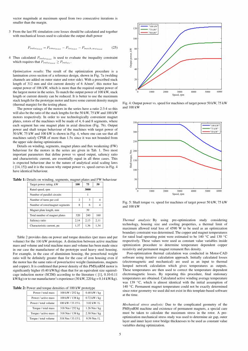
The power ratings of the motors in the series have a ratio 2:3:4 so thiswill also be the ratio of the stack lengths for the 50 kW, 75 kW and 100 kWmotors respectively. In order to use technologically convenient magnetplates, rotors of the machines will be made of 4, 6 and 8 segments, whereeach segment has one magnet plate in axial direction (Fig. 7b). Outputpower and shaft torque behaviour of the machines with target power of50 kW, 75 kW and 100 kW is shown in Fig. 4, where one can see that allmachines satisfy CPSR of more than 1.5x since it was not bounded fromthe upper side during optimization.

Details on winding, segments, magnet plates and flux weakening (FW)behaviour for the motors in the series are given in Tab. 1. Two mostimportant parameters that define power vs speed output, saliency ratioand characteristic current, are essentially equal in all three cases. Thisis expected behaviour due to the nature of analytical axial scaling laws( [14, 15]) and it is the reason why output power vs. speed curves in Fig. 4have identical behaviour.

Table 1: Details on winding, segments, magnet plates and FW behaviourTarget power rating, kW 100 75 50

Rated speed, rpm 3000

Number of parallel circuits 1

Number of turns per coil 2 3 4

Number of rotor/magnet segments 8 6 4

Magnet plate length, mm 39

Total number of magnet plates 320 240 160

Saliency ratio 2,14 2,13 2,11

Characteristic current, pu 1,37 1,36 1,34

Table 2 provides data on power and torque densities (per mass and pervolume) for the 100 kW prototype. A distinction between active machinemass and volume and total machine mass and volume has been made sincein our case the manufacturer of the prototype used heavy steel housing.For example, in the case of aluminium housing, the power/total weightratio will be definitely greater than for the case of iron housing even ifthe motor has the same ratio of power/active weight (laminations, magnetsand copper). It is confirmed that power density of this PMSynRM motor issignificantly higher (0.40 kW/kg) than that for an equivalent size squirrel-cage induction motor (SCIM) according to the literature ( [1], 0.10-0.11kW/kg) or to our manufacturer’s experience (30 kW, 220 kg = 0.14 kW/kg).

Table 2: Power and torque densities of 100 kW prototypePower / total mass 100 kW / 252 kg 0.40 kW / kg

Power / active mass 100 kW / 138 kg 0.72 kW / kg

Power / total volume 100 kW / 33.15 L 3.02 kW / L

Torque / total mass 318 Nm / 252 kg 1.26 Nm / kg

Torque / active mass 318 Nm / 138 kg 2.30 Nm / kg

Torque / total volume 318 Nm / 33.15 L 9.59 Nm / L

0 1000 2000 3000 4000 5000 6000

20

40

60

80

100

120

Speed, rpm

Out

put p

ower

, kW

0

"100 kW""75 kW" "50 kW"

Fig. 4: Output power vs. speed for machines of target power 50 kW, 75 kWand 100 kW

0 1000 2000 3000 4000 5000 6000

50

100

150

200

250

300

350

Speed, rpm

Shaf

t tor

que,

Nm

0

"100 kW""75 kW""50 kW"

Fig. 5: Shaft torque vs. speed for machines of target power 50 kW, 75 kWand 100 kW

Thermal analysis: By using pre-optimization study consideringtechnology, housing size and cooling properties, a thermal limit ofmaximum allowed total loss of 4590 W to be used as an optimizationboundary constraint was determined. The copper and magnet temperaturesfor rated load operating point were estimated to be 140 ◦C and 130 ◦Crespectively. These values were used as constant value variables insideoptimization procedure to determine temperature dependent copperresistivity and permanent magnet remanent flux density.

Post-optimization thermal calculation was conducted in Motor-CADsoftware using iterative calculation approach. Initially calculated losses(electromagnetic and mechanical) are used as an input to thermallumped network calculation which gives temperatures as outputs.These temperatures are then used to correct the temperature dependentelectromagnetic losses. By repeating this procedure, final stationarytemperatures are obtained. Calculated active winding average temperaturewas 139 ◦C, which is almost identical with the initial assumption of140 ◦C. Permanent magnet temperature could not be exactly determinedsince rotor geometry we used did not exist in this template-based softwareat the time.

Mechanical stress analysis: Due to the complicated geometry of thePMSynRM machine and existence of permanent magnets, a special caremust be taken to calculate the maximum stress in the rotor. A pre-optimization mechanical stress study was used to determine air gap, outerlayer and inner layer rotor bridge thicknesses to be used as constant valuevariables during optimization.

5

Fig. 6: Mechanical stress at 4500 rpm

The post-optimization stress analysis was preformed using 2D FEcalculation in COMSOL Multiphysics at the speed 50 % above rated speed(4500 rpm). In order to take into account the centrifugal force on the ironpart of the rotor, the load components were set parametrically using therelation

Fx = ρFeω2mx

Fy = ρFeω2my (26)

where ρFe is the density of the rotor material and ωm is the rotationalspeed of the rotor. Symmetry boundaries are used along the edges whererotor was cut to model the remainder of the rotor.

An additional stress to the rotor iron caused by the centrifugal force onthe magnets is taken into account as the pressure to the outer radial contactbetween magnet and rotor cavity. The pressure can be expressed as

Fy = ρPMω2m ·Ri (27)

where ρPM is the density of the permanent magnet material and Ri is thedistance between center of rotation and the ith magnet.

As it is shown in (26) and (27), the load forces depend only on squareof the rotational speed, assuming there is no significant deformation in thedisplacement (x and y). The rotor material was modelled using Young’smodulus (E = 200 GPa) and Poisson’s ratio (ν = 0.3). The maximal stressof 77.8 MPa occurred at one of the bridges, shown in Fig. 6. Yield strengthof 282 MPa was used to calculate safety factor ks=3.6. Due to the usageof the linear isotropic material in the solver and the assumption of smalldeformation, it is possible to recalculate maximal stress for the centrifugalloading at any speed

Snew =

(ωnew

ωcalc

)2

Scalc (28)

Using (28) it is possible to calculate maximum speed of the rotor for thedefined safety factor (ks).

ωmax = ωcalc

√Smax

ks · Scalc(29)

In this case, the theoretically highest speed for safety factor ks = 1 is8567 rpm.

Measurements: A 100 kW machine (IEC 180 frame size, forced aircooling) was built as a test prototype. A detail from manufacturing ofrotor segment before insertion of magnets is shown in Fig. 7b. Theprototype was tested in the laboratory equipped with 450 kW IPM loadmachine (Fig. 8) and ABB ACS800 Multidrive system. The details onprecision of measurement equipment are given in Tab. 3. In other words,the inverters for both the tested machine and the load machine aresharing the DC link which allows the energy between the motor (testedmachine) and the generator (load machine) to circulate while the lossesare supplied from the mains. Along with the measurement of electricalquantities, temperature, torque and speed, special measurement subsystemwas created for estimation of current control angle. Since inverters usedirect torque control (DTC), the exact position of current vector is notknown, therefore current waveform and rotor position from encoder wereused in order to decompose current vector into components to confirm

the calculated MTPA parameters. It was not possible to extract the exactvalue of magnet losses and mechanical windage and friction losses (themachine is cooled by an external fan) during load test. It was consideredthat these values are accurately calculated in the design stage. Therefore,the iron losses were determined as a difference between total measuredlosses, copper losses and estimated sum of magnet losses and friction andwindage losses.

The comparison of measured and calculated results is shown in Table 4.The difference in measured and calculated copper losses occurs primarilydue to the difference in measured and calculated current needed to producethe required shaft torque. The winding is made of Litz wire so proximityand eddy current losses are neglected although if the PWM shaped currentwaveform can be predicted in the design stage, those additional losses canbe accounted for, without the loss of generality of the presented approach.

The difference in measured and calculated iron losses is less than10 %, which can be considered a good match taking into account the keyuncertainties in iron loss calculation. The first uncertainty comes from thepower loss curves of steel lamination manufacturer which are normally notavailable for higher frequencies (5th or 7th harmonic with respect to ratedfundamental frequency of 200 Hz in this case). The second uncertaintycomes from the loss increase due to motor lamination manufacturingprocess: laser cutting or stamping. These processes severely deteriorateelectromagnetic properties of the electrical steel in the vicinity of statorslots and rotor cavities. The third uncertainty comes from PWM controland its effect on the current waveform shape and added harmonics in themagnetic field. These three influences are taken into the account by usinga correcting factor of 1.5 (experience based) which multiplies core lossescalculated using FE model. It is easy to conclude that if this factor wereonly 6.8 % larger (i.e. equal to 1.602), which is still realistic consideringthe current waveform shape of the inverter used, we would have obtained aperfect match in the calculation of core losses. Efficiency vs. speed curveat constant rated load 318 Nm is shown in Fig. 9, while power factor vs.speed is shown in Fig. 10.

(a) Lamination cross section (b) Rotor segment without magnets

Fig. 7: Manufactured prototype

Fig. 8: 100 kW prototype and 450 kW load machine

6

Table 3: Test-bench detailsSensor Type Accuracy

Torque HBM T40, 3000 Nm 0,05 %

Current ABB ES500-9647, 500 A 0,5 %

Voltage built-in LEM NORMA 4000 0,1 %

Speed encoder WACHENDORFF WDG 58B 0,01 %

500 1000 1500 2000 2500 3000 350060

65

70

75

80

85

90

95

100

Speed, rpm

Eff

icie

ncy

, %

measured

calculated

Fig. 9: Efficiency vs. speed curve at constant rated load 318 Nm

500 1000 1500 2000 2500 3000 35000.75

0.8

0.85

0.9

0.95

Speed, rpm

Po

wer

fac

tor

measured

calculated

Fig. 10: Power factor vs. speed curve at constant rated load 318 Nm

Table 4: Comparison of calculated and measured results at 100 kW, 3000 rpmCalculation Measurement Difference

T , Nm 317,9 318,3 0,1 %

I1, A 204,9 212,6 3,8 %

I , A 207,1 215,0 3,8 %

γ, ◦ -44,8 -39,9 -10,9 %

Pout, kW 99,9 100,0 0,1 %

Pel, kW 104,5 104,9 0,4 %

η, % 95,60 95,32 -0,3 %

Ploss, W 4597 4911 6,8 %

PCu, W 2016 2172 7,8 %

PFe, W 2522 2679 6,2 %

Pmag , W 35,7

Pmech, W 23,5

Conclusion: This paper presents a reliable and effective methodology foroptimizing a series of PMSynRMs using combined analytical-FE modelof the motor. It combines some of the best practices for definition and

execution of optimization problems found in literature with some originalcontributions presented in detail in the paper. Those already establishedpractices include definition of optimization variables as non-dimensionalratios, normalization of inequality constraints and their handling withoutusing penalty functions embedded into cost function, and optimizationwithout variation of the number of turns per coil and/or the number ofparallel paths.

The first contribution introduced in the paper is a time effective andaccurate method for calculation of peak transient stator winding short-circuit current to determine the level of demagnetization of permanentmagnets during sudden three-phase short circuit at the motor terminalsusing only magnetostatic FE calculations. This calculation is useful fordesigning fault tolerant motors. The second contribution is an accuratemethod for calculation of maximum power output at maximum speed usingmagnetostatic FE simulation considering the voltage and current limitsof the power supply and motor. The method is suitable for PMSynRMswith either finite or infinite theoretical maximum speed limit and is veryuseful for verifying whether or not the motor’s CPSR meets the designspecifications. Both methods are computationally efficient so they can beused for every population member of a stochastic optimization algorithm,like Differential Evolution used in this paper.

The optimization approach presented in the paper was used to designa PMSynRM rated 100 kW with excellent torque per volume capabilities,fitted into an IEC180 frame size housing previously used for an existing 2pole, 30 kW IE1 induction motor. A prototype was built and tested in orderto verify the calculation results by comparing them to measurements.

Acknowledgment: The research and prototype manufacturing has beensupported by electric machine manufacturing companies Koncar-MESd.o.o. and TEMA d.o.o.

References

1 A. de Almeida, F. Ferreira, and A. Quintino Duarte, “Technical andeconomical considerations on super high-efficiency three-phase motors,”Industry Applications, IEEE Transactions on, vol. 50, no. 2, pp. 1274–1285, March 2014.

2 A. de Almeida, F. Ferreira, and G. Baoming, “Beyond inductionmotors;technology trends to move up efficiency,” Industry Applications,IEEE Transactions on, vol. 50, no. 3, pp. 2103–2114, May 2014.

3 M. Barcaro, N. Bianchi, and F. Magnussen, “Permanent-magnetoptimization in permanent-magnet-assisted synchronous reluctancemotor for a wide constant-power speed range,” IEEE Transactions onIndustrial Electronics, vol. 59, no. 6, pp. 2495–2502, June 2012.

4 J. Haataja and J. Pyrhönen, “Permanent magnet assisted synchronousreluctance motor: an alternative motor in variable speed drives,” in EnergyEfficiency in Motor Driven Systems, F. Parasiliti and P. Bertoldi, Eds.Springer Berlin Heidelberg, 2003, pp. 101–110.

5 I. Boldea, L. Tutelea, and C. Pitic, “Pm-assisted reluctance synchronousmotor/generator (pm-rsm) for mild hybrid vehicles: electromagneticdesign,” IEEE Transactions on Industry Applications, vol. 40, no. 2, pp.492–498, March 2004.

6 P. Niazi, H. Toliyat, D.-H. Cheong, and J.-C. Kim, “A low-costand efficient permanent-magnet-assisted synchronous reluctance motordrive,” IEEE Transactions on Industry Applications, vol. 43, no. 2, pp.542–550, March 2007.

7 T. Tokuda, M. Sanada, and S. Morimoto, “Influence of rotor structureon performance of permanent magnet assisted synchronous reluctancemotor,” in International Conference on Electrical Machines and Systems,ICEMS, Nov 2009, pp. 1–6.

8 K. Khan, M. Leksell, and O. Wallmark, “Design aspects onmagnet placement in permanent-magnet assisted synchronous reluctancemachines,” in 5th IET International Conference on Power Electronics,Machines and Drives (PEMD), April 2010, pp. 1–5.

9 A. Vagati, B. Boazzo, P. Guglielmi, and G. Pellegrino, “Ferrite assistedsynchronous reluctance machines: A general approach,” in InternationalConference on Electrical Machines (ICEM), Sept 2012, pp. 1315–1321.

10 R. Vartanian, Y. Deshpande, and H. Toliyat, “Performance analysisof a rare earth magnet based nema frame permanent magnet assistedsynchronous reluctance machine with different magnet type andquantity,” in IEEE International Electric Machines Drives Conference(IEMDC), May 2013, pp. 476–483.

11 H. de Kock and M. Kamper, “Dynamic control of the permanentmagnet-assisted reluctance synchronous machine,” IET Electric PowerApplications, vol. 1, no. 2, pp. 153–160, March 2007.

12 S. Rick, M. Felden, M. Hombitzer, and K. Hameyer, “Permanentmagnet synchronous reluctance machine - bridge design for two-layer applications,” in IEEE International Electric Machines DrivesConference (IEMDC), May 2013, pp. 1376–1383.

7

13 S. Rick, A. Putri, D. Franck, and K. Hameyer, “Permanent magnetsynchronous reluctance machine; design guidelines to improve theacoustic behavior,” in International Conference on Electrical Machines(ICEM, Sept 2014, pp. 1383–1389.

14 D. Zarko and S. Stipetic, “Criteria For Optimal Design Of InteriorPermanent Magnet Motor Series,” in XXth International Conference OnElectrical Machines (ICEM), 2012, Sept 2012, pp. 1242–1249.

15 S. Stipetic, D. Zarko, and M. Popescu, “Scaling Laws for SynchronousPermanent Magnet Machines,” in Tenth International Conference onEcological Vehicles and Renewable Energies (EVER), 2015, April 2015,pp. 1–7.

16 R. Storn and K. Price, “Differential Evolution - a Simple and EfficientAdaptive Scheme for Global Optimization over Continuous Spaces,”Technical Report TR-95-012, ICSI, March 1995.

17 D. Zarko, D. Ban, and T. Lipo, “Design Optimization of InteriorPermanent Magnet (IPM) Motors with Maximized Torque Output in theEntire Speed Range,” in European Conference on Power Electronics andApplications, 2005, pp. 10 pp.–P.10.

18 W. Ouyang, D. Zarko, and T. Lipo, “Permanent Magnet Machine DesignPractice and Optimization,” in Conference Record of the 2006 IEEEIndustry Applications Conference, vol. 4, Oct 2006, pp. 1905–1911.

19 G. Sizov, D. Ionel, and N. Demerdash, “Multi-objective optimization ofPM AC machines using computationally efficient - FEA and differentialevolution,” in IEEE International Electric Machines Drives Conference(IEMDC), May 2011, pp. 1528–1533.

20 Y. Duan and D. Ionel, “A Review of Recent Developments in ElectricalMachine Design Optimization Methods With a Permanent-MagnetSynchronous Motor Benchmark Study,” IEEE Transactions on IndustryApplications, vol. 49, no. 3, pp. 1268–1275, May 2013.

21 P. Zhang, D. Ionel, and N. Demerdash, “Saliency Ratio and PowerFactor of IPM Motors Optimally Designed for High Efficiency and LowCost Objectives,” in IEEE Energy Conversion Congress and Exposition(ECCE), Sept 2014, pp. 3541–3547.

22 P. Zhang, G. Sizov, D. Ionel, and N. Demerdash, “Establishing theRelative Merits of Interior and Spoke-Type Permanent Magnet Machineswith Ferrite or NdFeB Through Systematic Design Optimization,” IEEETransactions on Industry Applications, vol. PP, no. 99, pp. 1–1, 2015.

23 Y. Duan and D. Ionel, “Nonlinear Scaling Rules for Brushless PMSynchronous Machines Based on Optimal Design Studies for a WideRange of Power Ratings,” IEEE Transactions on Industry Applications,vol. 50, no. 2, pp. 1044–1052, March 2014.

24 X. Liu and G. Slemon, “An Improved Method of Optimization forElectrical Machines,” IEEE Transactions on Energy Conversion, vol. 6,no. 3, pp. 492–496, Sep 1991.

25 J. Lampinen, “Multi-Constrained Nonlinear Optimization By TheDifferential Evolution Algorithm,” in 6th On-Line World Conference OnSoft Computing In Industrial Applications (Wsc6), 2001, pp. 1–19.

26 K.-C. Kim, J. Lee, H. J. Kim, and D.-H. Koo, “Multiobjective OptimalDesign for Interior Permanent Magnet Synchronous Motor,” IEEETransactions on Magnetics, vol. 45, no. 3, pp. 1780–1783, March 2009.

27 M. Martinovic, D. Zarko, S. Stipetic, T. Jercic, M. Kovacic, Z. Hanic,and D. Staton, “Influence of winding design on thermal dynamics ofpermanent magnet traction motor,” in International Symposium on PowerElectronics, Electrical Drives, Automation and Motion (SPEEDAM),2014, June 2014, pp. 397–402.

28 P. Zhang, G. Sizov, M. Li, D. Ionel, N. Demerdash, S. Stretz, andA. Yeadon, “Multi-Objective Tradeoffs in the Design Optimizationof a Brushless Permanent-Magnet Machine With Fractional-SlotConcentrated Windings,” IEEE Transactions on Industry Applications,vol. 50, no. 5, pp. 3285–3294, Sept 2014.

29 G. Pellegrino and F. Cupertino, “FEA-based Multi-ObjectiveOptimization of IPM Motor Design Including Rotor Losses,” inIEEE Energy Conversion Congress and Exposition (ECCE), Sept 2010,pp. 3659–3666.

30 N. Bianchi, D. Durello, and E. Fornasiero, “Multi-Objective Optimizationof a PM Assisted Synchronous Reluctance Machine, IncludingTorque and Sensorless Detection Capability,” in 6th IET InternationalConference on Power Electronics, Machines and Drives (PEMD 2012),March 2012, pp. 1–6.

31 M. Meyer and J. Bocker, “Transient peak currents in permanent magnetsynchronous motors for symmetrical short circuits,” in InternationalSymposium on Power Electronics, Electrical Drives, Automation andMotion, SPEEDAM, May 2006, pp. 404–409.

32 D. Zarko, D. Ban, and R. Klaric, “Finite Element Approach to Calculationof Parameters of an Interior Permanent Magnet Motor,” Automatika,vol. 46, no. 3–4, pp. 113–122, 2005.

33 W. L. Soong and T. J. E. Miller, “Field-weakening performance ofbrushless synchronous ac motor drives,” IEE Proceedings - ElectricPower Applications, vol. 141, no. 6, pp. 331–340, Nov 1994.

34 R. Schiferl and T. Lipo, “Power Capability Of Salient Pole PermanentMagnet Synchronous Motors In Variable Speed Drive Applications,”IEEE Transactions On Industry Applications, vol. 26, no. 1, pp. 115–123,1990.

8