of agriculture habitat production from - fs.fed.us · united states department of agriculture...

United StatesDepartment of AgricultureForest Service

Pacific SouthwestResearch Station

Research PaperPSW-RP-249

Economic Value of Big GameHabitat Production fromNatural and Prescribed Fire

Armando González-Cabán John B. Loomis Dana GriffinEllen Wu Daniel McCollum Jane McKeever Diane Freeman

Pacific Southwest Research Station

Forest ServiceU.S. Department of Agriculture

AbstractGonzález-Cabán, Armando; Loomis, John B.; Griffin, Dana; Wu, Ellen; McCollum, Daniel;

McKeever, Jane; Freeman, Diane. 2003. Economic value of big game habitat produc-tion from natural and prescribed fire. Res. Paper PSW-RP-249. Albany, CA: PacificSouthwest Research Station, Forest Service, U.S. Department of Agriculture; 38 p.

A macro time-series model and a micro GIS model were used to estimate a productionfunction relating deer harvest response to prescribed fire, holding constant other environ-mental variables. The macro time-series model showed a marginal increase in deerharvested of 33 for an increase of 1,100 acres of prescribed burn. The marginal deerincrease for the micro GIS model was 16. An additional 3,710 acres of prescribed burnwould produce an additional eight deer harvested regardless of the model. For an addi-tional 3,700 acres more of prescribed burn the marginal increase in deer harvested is fourand five deer respectively for the macro time-series and micro GIS models. Using theTravel Cost Method the change in consumer surplus or net willingness-to-pay was $257per additional deer harvested due to the additional trips in response to increasing deerharvest. The consumer surplus estimate using the Contingent Valuation Method was$222. Depending on the production function model used the initial deer hunting benefitresponse to a prescribed burning of 1,100 acres ranges from $3,840 to $7,920. An addition-al increase of 3,710 acres of prescribed burning would produce benefits of $1,920regardless of the model used. An extra 3,700 acres more would produce only between$960 and $1,200 depending on the model. When compared to the cost of conducting theprescribed burning, the benefits derived from an increase in deer harvest represent nomore than 3.4 percent of the total costs of the first 1,100 acres.

Retrieval terms: contingent valuation, deer hunting benefits, fire economics, prescribedburning costs, travel cost method, willingness-to-pay

The AuthorsArmando González-Cabán is Economist with the Pacific Southwest Research Station,USDA Forest Service, 4955 Canyon Crest Drive, Riverside, CA 92507. John B. Loomis isProfessor at the Department of Agricultural and Resource Economics, Colorado StateUniversity, Fort Collins, CO 80523. Dana Griffin and Ellen Wu at the time of the studywere graduate students at the Department of Agricultural and Resource Economics,Colorado State University, Fort Collins, CO 80523. Daniel McCollum is Economist withthe Rocky Mountain Research Station, 2150 Center Avenue, Fort Collins, CO 80526. JaneMcKeever is Wildlife Biologist with the California Department of Fish and Game, EasternSierra Inland Deserts Region, 330 Golden Shore, Suite 210, Long Beach, CA 90802. DianeFreeman is Wildlife Biologist with the San Bernardino National Forest, San JacintoDistrict Ranger, Idyllwild, CA 92349.

AcknowledgmentsWe thank Lucas Bair for research assistance regarding the cost of prescribed burning andeditorial assistance.

Thanks also to the California Department of Fish and Game for cover photographs: deerin the meadow (front) and the northern slope of Rouse Ridge in the San Jacinto RangerDistrict prescribed burn (front and back).

Publisher

Albany, CaliforniaMailing address:

PO Box 245, BerkeleyCA 94701-0245

(510) 559-6300

http://www.fs.fed.us/psw

April 2003

Contents

In Brief . . . . . . . . . . . . . . . . . . . . . . . . . . . . . . . . . . . . . . . . . . . . . . . . . . . . . . . . . . . . . . . iii

Introduction. . . . . . . . . . . . . . . . . . . . . . . . . . . . . . . . . . . . . . . . . . . . . . . . . . . . . . . . . . . . 1

Study Area . . . . . . . . . . . . . . . . . . . . . . . . . . . . . . . . . . . . . . . . . . . . . . . . . . . . . . . . . . . . 2

Two Production Function Modeling Approaches. . . . . . . . . . . . . . . . . . . . . . . . . . . 2

Literature Review. . . . . . . . . . . . . . . . . . . . . . . . . . . . . . . . . . . . . . . . . . . . . . . . . . . . . . . 3Deer Habitat and Prescribed Burning . . . . . . . . . . . . . . . . . . . . . . . . . . . . . . . . . . 3Geographic Information Systems . . . . . . . . . . . . . . . . . . . . . . . . . . . . . . . . . . . . . . 3Multiple Regression Models for Estimating the Production Function. . . . . . . 4Economic Evaluation. . . . . . . . . . . . . . . . . . . . . . . . . . . . . . . . . . . . . . . . . . . . . . . . . 5

Production Function Modeling Approaches . . . . . . . . . . . . . . . . . . . . . . . . . . . . . . . 6Time-Series, Macro Scale Production Function . . . . . . . . . . . . . . . . . . . . . . . . . . 6Micro GIS Approach to Estimating the Production Function . . . . . . . . . . . . . . 7Description of GIS-Based Micro Regression Variables . . . . . . . . . . . . . . . . . . . . 9

Estimated Production Functions. . . . . . . . . . . . . . . . . . . . . . . . . . . . . . . . . . . . . . . . . . 9Macro Time-Series San Jacinto Ranger District Equations . . . . . . . . . . . . . . . . . 9San Jacinto Ranger District Log-Log Model . . . . . . . . . . . . . . . . . . . . . . . . . . . . 10Summary of Micro Regressions Based on GIS Analysis . . . . . . . . . . . . . . . . . . 11Percent of Hunting Location Area Burned, Micro Model. . . . . . . . . . . . . . . . . 11Micro GIS-Based Equation Using Total Acres Burned . . . . . . . . . . . . . . . . . . . 11Micro GIS-Based Equation Using OLS Log-Log Form of

Harvest Per Acre . . . . . . . . . . . . . . . . . . . . . . . . . . . . . . . . . . . . . . . . . . . . . . . . . 12

Applying the Regression Production Functions . . . . . . . . . . . . . . . . . . . . . . . . . . . 14Applying Results of Macro Time-Series Production Function Model . . . . . . 14Applying Results of Micro GIS Production Function Model. . . . . . . . . . . . . . 14

Valuation of Deer Hunting . . . . . . . . . . . . . . . . . . . . . . . . . . . . . . . . . . . . . . . . . . . . . 15Valuation Methodologies . . . . . . . . . . . . . . . . . . . . . . . . . . . . . . . . . . . . . . . . . . . . 15CVM and TCM Comparisons . . . . . . . . . . . . . . . . . . . . . . . . . . . . . . . . . . . . . . . . 18

Data for TCM and CVM Models . . . . . . . . . . . . . . . . . . . . . . . . . . . . . . . . . . . . . . . . 19Survey Mailing and Response Rate . . . . . . . . . . . . . . . . . . . . . . . . . . . . . . . . . . . 19Descriptive Statistics . . . . . . . . . . . . . . . . . . . . . . . . . . . . . . . . . . . . . . . . . . . . . . . . 19

iUSDA Forest Service Research Paper PSW-RP-249. 2003.

Economic Value of Big GameHabitat Production from Naturaland Prescribed FireArmando González-Cabán John B. Loomis Dana GriffinEllen Wu Daniel McCollum Jane McKeever Diane Freeman

Pacific SouthwestResearch Station

USDA Forest ServiceResearch PaperPSW-RP-249

April 2003

Statistical Results of TCM and CVM Valuation Models . . . . . . . . . . . . . . . . . . . 20Travel Cost Method . . . . . . . . . . . . . . . . . . . . . . . . . . . . . . . . . . . . . . . . . . . . . . . . . 20Contingent Valuation Method . . . . . . . . . . . . . . . . . . . . . . . . . . . . . . . . . . . . . . . . 22Comparing the Consumer Surplus from TCM and CVM . . . . . . . . . . . . . . . . 22

Applications of Values to Estimate Benefits of Prescribed Burning. . . . . . . . . 23Comparison to Costs . . . . . . . . . . . . . . . . . . . . . . . . . . . . . . . . . . . . . . . . . . . . . . . 24

Conclusion . . . . . . . . . . . . . . . . . . . . . . . . . . . . . . . . . . . . . . . . . . . . . . . . . . . . . . . . . . . . 24

References . . . . . . . . . . . . . . . . . . . . . . . . . . . . . . . . . . . . . . . . . . . . . . . . . . . . . . . . . . . . 26

Appendix I. Survey Instrument Used in the Study . . . . . . . . . . . . . . . . . . . . . . . . 29

Appendix II. San Bernardino National Forest, San Jacinto Ranger District . . . . . . . . . . . . . . . . . . . . . . . . . . . . . . . . . . . . . . . . . . . 37

ii USDA Forest Service Research Paper PSW-RP-249. 2003.

In Brief González-Cabán, Armando; Loomis, John B.; Griffin, Dana; Wu, Ellen; McCollum, Daniel;

McKeever, Jane; Freeman, Diane. 2003. Economic value of big game habitat produc-tion from natural and prescribed fire. Res. Paper PSW-RP-249. Albany, CA: PacificSouthwest Research Station, Forest Service, U.S. Department of Agriculture; 38 p.

Retrieval terms: contingent valuation, deer hunting benefits, fire economics, prescribedburning costs, travel cost method, willingness-to-pay

On the San Jacinto Ranger District (SJRD) of the San Bernardino National Forestin southern California prescribed burning is an important resource managementprogram. Prescribed burning is used to provide many multiple use benefitsincluding improved deer habitat, opportunities for dispersed recreation, andreduced hazardous fuels in the chaparral that surround several residential com-munities and associated watersheds.

The main objective of this research was to quantify the economic value of theimproved deer hunting resulting from prescribed burning. Previous prescribedfirework has shown that fire positively enhances deer habitat. Enhanced deerhabitat increases deer population hence better hunting. Two approaches wereused to estimate a production function relating deer harvest response to pre-scribed burning, holding constant other environmental variables. We compareda macro level, time-series model that treated the entire SJRD as one area, and amicro geographic information system (GIS) model that disaggregated the RangerDistrict into the 37 hunting locations reported by hunters. Both modelingapproaches gave somewhat mixed results in that some statistical specificationsshowed no statistically significant effect of prescribed burning. However, thebetter fitting (68 percent of variation explained) log-log model functional form ofthe macro time-series model did show a statistically significant effect of the com-bined prescribed fire and wildfire acres on deer harvest over the 20 year periodof 1979-1998.

All technical information on prescribed fire and fire effects was obtainedfrom USDA Forest Service personnel in the SJRD and California Department ofFish and Game and was used in development of the hunter’s survey question-naire used in this work.

During the 1999 deer hunting season, a mail questionnaire was sent to arandom sample of deer hunters with licenses for deer in Zone D19, whichincludes the SJRD. Of the 762 questionnaires mailed to deer hunters inCalifornia, a total of 356 deer hunters’ responses were collected after two mail-ings for a response rate of approximately 47 percent.

Two of the three micro GIS model specifications showed that the initial effectof prescribed burning on deer harvest in the 37 hunting locations within theSJRD was statistically significant. Lagged effects of prescribed burning wereconsistently insignificant in our models, suggesting that most of the responseoccurs in the year of the burn. The macro time-series model estimated a largerresponse to burning of the first 1,100 acres than the micro GIS model did; but forincreases in fire of more than 1,100 acres, the two models provided nearly iden-tical estimates.

The net economic value of the resulting additional deer hunting benefitswas estimated by using the Travel Cost Method (TCM) and the ContingentValuation Method (CVM). By using TCM analysis, we found the change in con-sumer surplus or net willingness-to-pay (WTP) is $257 per additional deerharvested due to the additional trips the hunter took in response to increasingdeer harvest. From CVM, we found the change in consumer surplus of $222 peradditional deer harvested. The mid-point marginal consumer surplus of TCMand CVM, therefore, is $240 per deer harvested.

iiiUSDA Forest Service Research Paper PSW-RP-249. 2003.

The initial deer hunting benefit response to the current magnitude of pre-scribed burning of 1,100 acres ranges from $3,840 to $7,920, depending on themodel. However, the incremental gains for additional prescribed burning arequite similar across models: the annual economic hunting benefits of increasingprescribed burning from its current magnitude of 1,100 acres to 4,810 acres is$1,920, regardless of the model used. Likewise, for a second increase of 3,700acres of prescribed burning to 8,510 acres, the deer hunting benefits are calculat-ed to be between $960 and $1,200 each year, which are fairly similar despite thedifferent modeling approaches.

The costs of prescribed burning on the San Bernardino National Forest rangefrom $210 to $240 per acre. Using the information in this research, the full incre-mental costs of burning the first 1,100 acres would be $231,000, with eachadditional 3,710 acres burned costing $779,100. The deer hunting benefits repre-sent at most about 3.4 percent of the total costs of the first 1,100 acres ofprescribed burning. This finding can be used in two ways. First, the incrementalcosts of including deer objectives in a prescribed burn of 1,100 acres should notexceed $8,000, as the incremental benefits are no larger than this. Second, theother multiple use benefits—such as watershed, recreation, and the hazard fuelreduction benefits to adjacent communities—would need to make up the differ-ence if the prescribed burning program is to pass a benefit-cost test. For example,if prescribed burning 1,100 acres prevented as few as two residential structuresfrom burning, the prescribed burning program would likely pass a benefit-costtest. However, such an assessment was beyond the scope of this study.Nonetheless, we can conclude that incremental deer-hunting benefits from pre-scribed fire appear to be relatively small, compared to the cost of prescribedburning in the SJRD.

iv USDA Forest Service Research Paper PSW-RP-249. 2003.

IntroductionEstimating the impact of fire on resources and the economic consequences of itis very difficult. This difficulty arises because of the multiple outputs of the for-est and the strong interdependence between the present output choice and thecapital stock level of natural resources (González-Cabán 1993). The problem isfurther complicated because the effects of fire on the production stream of manygoods and services from the forest, particularly nonmarket outputs, is largelyunknown (SAF 1985).

This research makes a methodological contribution to the development ofmodels for evaluating ecological effects of fire as well as providing results for theSan Jacinto Ranger District (SJRD) in the San Bernardino National Forest locat-ed in southern California. In her recent review of the economics of prescribedburning, Hesseln (2000) posed the problem as “a lack of economic models toevaluate short-and long-term ecological benefits of prescribed fire. Withoutunderstanding the relationship between economic outcomes and ecologicaleffects, it will be difficult to make effective investment decisions. Researchshould focus on defining a production function to identify long-term relation-ships between prescribed burning and ecological effects. Identifying productionfunctions relationships will form the basis for future cost-benefit analysis withrespect to prescribed burning …” (Hesseln 2000, p. 331-332). To make a firstmodest step in the direction suggested by Hesseln, this study estimates produc-tion relationships between prescribed burning and deer harvest by usingtime-series data and geographic information system (GIS) approaches. Previouswork has shown an increase in deer population as a result of forage qualityimprovement from burning their habitat (Klinger and others 1989). The modelsdeveloped were then used to predict the resulting increases in deer harvest fromprescribed burning and, subsequently, to measure the economic benefits of thisenvironmental improvement (increase in deer harvests) using nonmarket valu-ation techniques.

The SJRD is located in southern California’s San Bernardino National Forestbetween Palm Springs and Idyllwild, California. As noted by the USDA ForestService: “Some of the best deer hunting in Riverside County is found in thisarea. It is also a very valuable watershed that includes the South Fork of theSan Jacinto River” (Gibbs and others 1995, p. 6). The SJRD is an ideal area todemonstrate and compare different approaches to estimating a production func-tion between prescribed burning and deer harvest, because prescribed fire hasbeen used for more than 20 years to stem the long-term decline in deer popula-tions since the 1970s (Gibbs and others 1995, Paulek 1989). Previous research onprescribed burning shows that fire positively enhances deer habitat and popula-tions (CDFG 1998), but the economic benefits have not been quantified. TheUSDA Forest Service has a detailed database of fire history for this area predat-ing the 1970s. The California Department of Fish and Game (CDFG) has hunterdeer-harvest records for the SJRD back to 1974. These two agencies provide thefundamental data sets for modeling a relationship between deer harvest andfire, whether prescribed burns or wildfires. Information from our analysis maybe relevant to policy because the SJRD plans to increase the amount of pre-scribed burning by 50 to 100 percent over the next few years (Gibbs and others1995, Walker 2001).

The positive effect of prescribed fire on enhancing deer habitat and popula-tions has been shown (CDFG 1998, Klinger and others 1989), but the resultingeconomic benefits of the treatments have not been quantified. We hypothesizedthat prescribed burning has a systematic positive effect on deer harvest and willuse two nonmarket valuation methods to estimate the economic value of addi-tional deer harvest.

USDA Forest Service Research Paper PSW-RP-249. 2003. 1

Study AreaIn general, southern California is characterized by a Mediterranean climate, withhot and dry summers and cool, humid winters. There is a significant amount ofvariation in temperatures and local site conditions in the SJRD. Elevation in theSJRD ranges from 3,500 feet up to 10,800 feet. Below 5,000 feet elevation, thedominant vegetation within the SJRD is chaparral. Annual rainfall for the chap-arral biome is approximately 15 to 16 inches. Areas higher than 5,000 feet tend tobe dominated by hardwoods and conifers, such as live oak and Douglas-fir, withannual rainfall reaching up to 30 inches.

Within the SJRD, primarily the USDA Forest Service manages the land, withsmall amounts of land administered by the Bureau of Land Management (BLM)as well as the State of California. Mount San Jacinto State Park lies on the north-eastern boundary of the SJRD and is owned by the State of California. There aretwo state game refuges, one located in the Mount San Jacinto State Park and theother in the southern portion of the Ranger District around the Santa RosaMountains. Hunting is prohibited within the refuges.

The SJRD is an area that evolved with fire as a natural environmental factor.Declining abundance of successional vegetation communities is considered tohave the greatest long-term effects on deer populations (CDFG 1998).Historically, fire, either prescribed or natural, has been the primary mechanismfor establishing these vegetation communities. Studies in California have notedthat after a burn, increased deer numbers can be attributed to individuals mov-ing into the area to feed (Klinger and others 1989). These increased deer numbershave been thought to improve reproduction due to increased forage quality andan increase in fawn survival rates. The CDFG has noted a significant increase inbuck harvest from 1987 to 1996 in hunt locations that had large fires versus huntlocations that did not have large fires (CDFG 1998). To improve deer habitat inCalifornia, controlled burns have been underway in all the major parks andforests for many years (Kie 1984). Efforts including controlled burning to removebrush have been part of a program to create desirable deer habitat (i.e., chapar-ral in the open scrubland) and to mitigate the loss of deer habitat resulting fromcommercial and residential development.

Two Production Function ModelingApproachesTo test whether prescribed burning has a systematic effect on deer harvest weused a macro or aggregate time-series approach and a micro, spatial approach.To estimate the economic value of additional harvest resulting from prescribedburning treatments we used two nonmarket valuation methods. By examiningprescribed burning effects on deer harvest with two different approaches—amacro or aggregate time-series approach and a micro, spatial approach (e.g.,GIS)—comparisons can be made between the results for consistency betweenthese two approaches. A macro approach would be able to test the effects of fire,prescribed and natural, across the entire study area over a long period of time.Although more aggregate in geographic space, data availability allows us tocover a longer time frame, and hence test long dynamic effects. Using a microapproach provides greater spatial detail to elements such as the influence of ameadow or ridge, but a less temporal time frame is covered because of data lim-itations. Thus, each approach to estimating the production function has itsrelative strengths and weaknesses.

USDA Forest Service Research Paper PSW-RP-249. 2003.2

Literature ReviewDeer Habitat and Prescribed Burning There have been just a few studies indicating the positive results of fire on deerhabitat and populations. In one northern California study it was reported thatthe number of deer in stands of pure chaparral that were burned by fire quadru-pled during the first growing season after the burn, then gradually decreased topre-burn levels over the next 4 years (Klinger and others 1989). These increaseddeer numbers were attributed to the movement of deer into the burned standswhere forage quality was improved and fawn survival rate was up. Using pre-scribed fire to benefit deer should occur during the season when the greatestlikelihood of achieving the desired plant response will occur. According to theCDFG, dry season burns tend to result in better regeneration of shrub speciesfrom seed than wet season burns. Fire adapted shrub species, such as chaparral,respond best to prescribed burns during the time of year when fire occurs natu-rally, usually in late summer or early fall.

In arid regions such as southern California, vegetation change does notconform to traditional patterns. Vegetation is always in a state of flux due toharsh environmental factors and extreme events such as fire that cause a sud-den shift in vegetation composition. Fire can cause the germination of seedsthat would otherwise be dormant and create changes in relative abundance ofvegetation such as chaparral. In the southern California area, there are differ-ent types of chaparral: seeding species and sprouting species. According to apast study (Zedler and others 1983) on the impacts of fire in chaparral, firescan produce a varying degree of results depending on the species of chaparral.This implies that fire regimes in chaparral produce a variety of responses invegetation communities depending upon the type of species that exist (Zedlerand others 1983). In terms of deer harvest, this difference in chaparral vegeta-tion may suggest that certain areas will be more productive for hunting after afire, depending on what type of vegetation was burned, e.g., the sprouting orseeding species. The biotic zonation in the San Jacinto Mountains where theSJRD is located includes coastal sage scrub up to 2,500 feet, hard (lower andupper) chaparral from 2,500 to 5,000 feet, yellow pine forest from 5,000 to 8,000feet, lodgepole pine forest from 8,000 to 9,500 feet, and subalpine and alpineforest from 9,500 to 11,000 feet.

Prescribed burns have become a management tool for improving chaparralfor deer habitat. As a result, the use of prescribed fire has become a technicallyviable solution for improving the carrying capacity of chaparral deer ranges suchas those in southern California. Hence, it is important to document and quantifythe magnitude of the benefits from prescribed burning compared to its costs.

Deer hunting is considered a necessary element of deer management (Paulek1989). Hunting is a tool to restrict deer herds to the carrying capacity of theirrange. This type of herd restriction prevents “boom or bust” cycles among pop-ulations and helps maintain a balance of forage across a deer herd’s range. Deerhunting also provides economic activity to local economies in California. Arecent study using survey data compared the economic contribution of deerhunting in 1997 to a previous survey in 1987 in northeastern California. Theresults indicated that hunters’ expenditures (not adjusted for inflation) in Lassen,Modoc, and Plumas counties have dropped significantly, from $5.4, $4.7, and$0.76 million, respectively, in 1987 to $0.83, $0.55, and $0.17 million, respective-ly, in 1997 (Loft, 1998). Nonetheless, even in 1997, deer hunters in these threecounties still accounted for an estimated $1.5 million in local expenditures.

Geographic Information SystemsA geographic information system (GIS) is a system for working with spatialdata. The Environmental Systems Research Institute (ESRI) (1995) describes GIS


as an organized collection of computer hardware, software, geographic data,and personnel designed to efficiently capture, store, update, manipulate, ana-lyze, and display all forms of geographically referenced information.

GIS can also be described by its ability to carry out spatial operations,known as queries, through linking different data sets together. These functionsare what make a GIS a powerful tool for data analysis. Typically, a GIS linksdifferent data sets to reveal some new or unknown relationship (Chou 1997).For example, in the case of fires, it is possible through a GIS to discover howmany acres were burned in a particular region by examining overlaying datasetsin a spatial context.

In order to design a digital database, some key questions must be answered:What will be the study area or boundary? What types of data files or layers(e.g., vegetation cover, prescribed burned areas, roads, etc.) will be needed inorder to solve the problem? What attributes are needed for each layer and howwill these attributes be stored? After these questions are answered, then spatialdata should be obtained for inputting into the database and making it usable.The last part of building a spatial database involves specifying what necessaryattribute information will be needed by the various data layers and then addingit on. This is usually done by relating a common item or joining the attributesonto a particular data layer.

Multiple Regression Models for Estimating theProduction FunctionEstimating a production function that relates deer harvest to acres of prescribedburning must also control for other inputs that influence the production of deerfor harvest. This includes wildfire, elevation (used as a proxy for vegetationdata that was incomplete), total precipitation, temperature, and distance toroads. Thus, multiple regression analysis is an appropriate technique. The sim-plest form used in this study is ordinary least squares regression. This can beimproved upon for modeling deer harvest, especially at the micro level whereharvest in any small spatial unit is a non-integer variable, by using a count datamodel. Count data models are based on probability distributions that have massonly at non-negative integers, and it is impossible for the distribution to have afractional outcome or a negative outcome (Hellerstein 1992). This is certainlythe case of deer harvest, as hunters cannot harvest a fraction of a deer. The clas-sic example of a count distribution is the Poisson process. The counts describedconsist of numerical quantities, Lambda, which is the mean number of eventsper unit of progression (specified as an exponential link function that ensuresnonnegativity) and is equal to the variance. As Lambda increases, the Poissondistribution approaches the normal distribution, with a decreasing probabilitymass at zero (Forsythe 1999).

Given the stringency of the mean variance equality restriction imposed bythe Poisson distribution, a more generalized count model, such as the negativebinomial distribution, is often more consistent with the data. The negative bino-mial version allows the variance to move freely. Both the Poisson and thenegative binomial distributions yield the equivalent of a semi-log form wherethe log of the dependent variable is regressed against the explanatory variables.

Using ordinary least squares (OLS), it is not possible to take the log of azero-valued observation of the dependent variable; but if the negative binomialcount data model is used, the probability distribution allows for this—similar toa non-linear least squares that avoids the need for transformations (Hellerstein1992). Therefore, these features make the Poisson and negative binomial distri-butions useful in our micro GIS-based analysis since the variable we are tryingto explain—deer harvest in 1 of 37 sub-hunting location areas—is a non-negativeinteger. The number of harvested deer recorded in specific hunting areas tends


to be small, such as 0, 1, and 2 or 3, rather than larger numbers like 10, 20, or 50.Therefore, the count data is more efficient with the distribution mass at smallintegers than OLS (Hellerstein 1992).

However, when modeling the aggregate harvest for all of the SJRD, themean number of deer harvested is much larger and varies between 80 and 157deer in any given year; therefore, using OLS is an acceptable approach for themacro time-series modeling.

Economic EvaluationWildlife such as deer are commonly considered nonmarket goods in much ofthe western United States. Although natural resources have both use andnonuse values (e.g., existence values), the widespread distribution of deer sug-gests that the incremental benefits of more deer are use values. For deer, usevalues are those associated with tangible uses in recreational hunting or view-ing benefits. Because of difficulty in identifying deer viewers, this study focuseson deer hunters.

Kahn (1995) categorizes two major techniques for estimating nonmarketgoods: indirect and direct techniques. Indirect techniques (revealed preferenceapproaches) can be used to analyze decisions or actions in response to changesin an environmental amenity to reveal the value of the amenity. Indirect tec-niques such as hedonic pricing and travel cost models are mostly useful forestimating the use value of nonmarket goods. Direct valuation techniques elic-it values (stated preference approaches) from individuals through surveymethods, which can be used to measure both use and nonuse values. In thisstudy, we will apply both the Contingent Valuation Method (CVM) and theTravel Cost Method (TCM) to estimate the use-value in deer hunting. Althoughthere is a substantial amount of literature comparing TCM and CVM estimatesof the value of a recreation day (Carson and others 1996), there are fewer com-parisons for a change in recreation quality.

Production Function Modeling Approaches Two primary methods for estimating a deer harvest production function wereapplied in this study. Both methods were looking for a statistical relationshipbetween deer harvest and fire, both wildfires and prescribed fires, that occurredin southern California’s SJRD. The distinguishing difference between the twomethods applied is the variation in spatial scale. The GIS-based approach canbe considered a micro, spatial scale examination, while the macro time- seriesapproach looks at the entire SJRD at a more aggregate level, using the entireranger district as one unit of observation in each year. This more aggregate ormacro method tests a time-series relationship between deer harvest and fire inSJRD. The GIS-based method disaggregates fewer years of fire data and deerharvest into a much finer level of spatial detail, breaking the SJRD into the 37hunting locations reported by hunters (see appendix II for a general map ofSJRD).

Time-Series, Macro Scale Production Function The first statistical approach is based on a time-series regression model to testfor a relationship between deer harvest (the dependent variable) and prescribedfire, controlling for other independent variables such as annual precipitationand temperature during the hunting season (table 1). This approach used adataset for SJRD, provided by the CDFG and the USDA Forest Service. The firerecords provided data from 1975 for natural wildfire but only from 1979 forprescribed burns within the SJRD. This ranger district represents the majority ofpublicly accessible land for deer hunting in Riverside County. Deer harvestdata from 1975 were provided by CDFG.


A time-series model was established with this data and weather informationfrom the University of Nevada at Reno’s Western Climate Center database thatcontains temperature and precipitation data from the SJRD dating back to 1975.The model attempts to directly explain deer harvest within the SJRD as a func-tion of wildfire, prescribed fire, temperatures during the October huntingseason, and total precipitation in a given year (table 1).

The full model (equation 1) is given, and then a lagged model (equation 2)is included that allows for harvest to be sensitive to previous years’ prescribedfire and wildfire. In past research, the use of burned areas by deer has beenshown to increase dramatically during the subsequent years (Klinger and oth-ers 1989). Therefore, this model takes into account these subsequent years byusing lagged variables.

The SJRD time-series production function model is:

[1] SJRD deer harvest in yeart = func (RxFiret, WildFiret, TotPrecipt,OctTempt, Yeart)

RxFiret is the acres of prescribed fire in year t, WildFiret is the acres of wild-fire in year t, TotPrecipt is the sum of precipitation for year t, OctTempt is thetemperature in October during the hunting season, and Yeart is a trend variable,with 1975 = 1, 1976 = 2, etc.

The SJRD time-series production function lagged model is:

[2] SJRD deer harvest in yeart = func (RxFiret-1, WildFiret-1, TotPrecipt,OctTempt, Yeart)

Using the log-log form represents the non-linear forms of equations 1 and 2.This format allows for a non-linear relationship, and the coefficients for fire canbe interpreted as elasticities: the percent change in deer harvest with a 1 percentchange in acres burned.

Micro GIS Approach to Estimating the ProductionFunctionThe second statistical approach taken in this study focused on using a GIS forintegrating spatial data into an economic relationship. A similar multiple regres-sion approach was used as in the first method, except that the study area wasdivided into 37 individual hunting locations reported by hunters (see appendix I).Thus, the primary distinction to the macro time-series model is that with theGIS-based micro model, deer harvest was modeled for 37 smaller hunting loca-tions instead of by using just one large hunting zone that encompassed the SJRD.This allowed for the incorporation of other influences on deer harvest that var-ied spatially across individual hunting locations such as distance to roads andelevation.

All of the spatial data for this method came either from the United StatesGeological Survey (USGS) 1:100,000 digital line graphs (DLG) files or from theUSDA Forest Service Arc/Info and Arc/View files, which were provided by theSan Bernardino National Forest Supervisor’s Office. The data for all the files usethe Universal Transverse Mercator (UTM) coordinate system (Zone 11, DatumNAD 27). The scale of the data is at 1:250,000. These spatial data files contain pre-scribed fire, wildfire, elevation, roads, and trails information. The CDFG mapsand tally sheets provided the hunting location information. The areas on theCDFG maps were aligned with areas on USGS 7.5 minute topographical quads.

The function of the GIS portion of this project was to provide the detaileddata at a micro level, which could be used to regress the relationship betweendeer harvest and prescribed fire or wildfire. Using a spatial database to identify


Table 1—Data for macro time-series production function model.

Acres BurnedYear SJRD-Harvest Prescribed Fire Wildfires Oct-Temp Annual

Precipitation

No. Deer °F inches1975 105 NA1 5231 70.48 19.941976 145 NA 0 69.23 27.221977 113 NA 3948 74.32 22.631978 101 NA 2049 74.32 46.991979 148 40.00 1987 70.73 29.621980 139 194.10 3,7627 73.68 45.651981 155 291.90 1,5016 67.00 15.811982 157 228.00 6279 69.42 49.471983 143 3,119.90 7206 69.52 56.871984 120 971.00 13 64.42 16.961985 119 1,311.80 2,1128 67.29 23.581986 162 1,309.00 0 65.19 23.921987 131 181.50 1432 69.58 23.491988 103 1,954.00 1615 75.52 18.251989 128 2,009.60 2121 68.65 15.981990 104 423.00 119 74.19 19.121991 83 0.00 91 72.19 31.491992 117 77.70 1458 70.00 23.441993 93 383.00 269 69.13 43.641994 132 25.40 2,2416 66.68 20.841995 82 975.20 7116 73.84 45.091996 131 822.00 1,2338 68.10 28.361997 126 4.94 NA 69.06 24.961998 99 0.00 NA NA 28.47

1NA=not available

and describe a spatial pattern and distribution between deer harvest and fires isvery useful. The focus of building a GIS was to provide data on variables toestimate the deer production function.

The first step was to identify the necessary layers needed to run a regressionbetween deer harvest and fires. A hunting layer was constructed for the regres-sion model, which contains deer harvest by hunting locations. Then layers wereadded for the independent variables, including prescribed burn, wildfire, aver-age elevation, temperature, distance to trails, dirt roads and roads from eachhunting location, and distance to wildfires from each hunting location.Vegetation type would have been desirable, but this information was incom-plete and will not be completed for the entire area until the distant future.

The next step in constructing a spatial model is deciding on how to deter-mine the delineation of geographic units (Chou 1997). Decisions on size ofgeographic units must balance consistent data availability as well as meaningfulunits. Although a 640-acre section grid had some attractive features, deer harvestdata at that level of resolution was only available for 4 years. Further, deer herdmovement may often be larger than a 640-acre section. Therefore, we relied upondeer harvest locations reported by hunters within the SJRD. These hunt locationsare defined by topographic features, such as streams, steep ridgelines, or some-times features created by people, including towns or major roads. Theselocations were often much larger than a single section and encompassed areas


where deer herds and hunters might move within but not between areas. In addi-tion, CDFG had a much longer time-series of deer harvest at the harvest locationlevel as compared to the section level. Because of the different size of each harvestlocation, some basic assumptions had to be made when calculating distances toroads, trails, or recently burned areas. These assumptions included finding a cen-tral point within each harvest location to serve as a point to calculate distances.Therefore, all distance calculations are based on averages from a central point. Inaddition, regressions accounted for the size of the hunting location as one of theexplanatory variables.

All relevant GIS data had to be exported into spreadsheet format and pre-pared for regression analysis. A count data model was estimated that regresseddeer harvest per hunting zone against prescribed fire and wildfire burned from1975 to 1998.

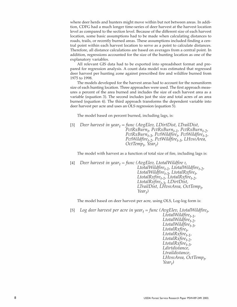
The models developed for the harvest areas had to account for the nonuniformsize of each hunting location. Three approaches were used. The first approach meas-ures a percent of the area burned and includes the size of each harvest area as avariable (equation 3). The second includes just the size and total acres of an areaburned (equation 4). The third approach transforms the dependent variable intodeer harvest per acre and uses an OLS regression (equation 5).

The model based on percent burned, including lags, is:

[3] Deer harvest in yeart = func (AvgElev, LDirtDist, LTrailDist, PctRxBurnt, PctRxBurnt-1, PctRxBurnt-2, PctRxBurnt-3, PctWildfiret, PctWildfiret-1, PctWildfiret-2, PctWildfiret-3, LHvstArea, OctTempt, Yeart)

The model with harvest as a function of total size of fire, including lags is:

[4] Deer harvest in yeart = func (AvgElev, LtotalWildfire t, LtotalWildfiret-1, LtotalWildfiret-2, LtotalWildfiret-3, LtotalRxfiret, LtotalRxfiret-1, LtotalRxfiret-2, LtotalRxfiret-3, LDirtDist, LTrailDist, LHvstArea, OctTempt, Yeart)

The model based on deer harvest per acre, using OLS, Log-log form is:

[5] Log deer harvest per acre in yeart = func (AvgElev, LtotalWildfiret,LtotalWildfiret-1, LtotalWildfiret-2, LtotalWildfiret-3, LtotalRxfiret, LtotalRxfiret-1, LtotalRxfiret-2, LtotalRxfiret-3, Ldirtdistance, Ltraildistance, LHvstArea, OctTempt, Yeart)


Description of GIS-Based Micro Regression VariablesElevations (AvgElev) (meters) are based on USGS digital elevation models(DEMs) and act as a proxy for vegetation types that were not available.However, we do not have an expected sign on elevation, but simply wish tocontrol for elevation differences between the 37 individual hunting areas with-in the SJRD. Both fire variables, wildfire (WildFire) and prescribed fire (RxBurn)(total acres/year), are expected to have a positive sign (Kie 1984, Zedler andothers 1983).

The distance (meters) to road (LDirtDist) and trail (LTrailDist) variables arebased on the distances from a central point in each hunting location. Two argu-ments can be made about the sign’s direction. One argument is based onaccessibility for hunters, in which having a close proximity to either a trail orroad would make hunting easier, more desirable, and would positively affectdeer harvest. The second argument is based on the intrusion of deer habitat bya road or trail. This perspective would lead to a decline in deer harvest becauseroads cause a break in habitat and pose a threat. Therefore, the expectation isambiguous.

The distance (meters) to fire variable (LDistFire) is a measure of how closefire comes to burning into the interior of the hunting area’s vegetation. A valueof zero would indicate a fire in that year burned into the center of the hunt area.This variable sign may be either positive or negative.

Harvest area (LHvstArea) (acres) accounts for the size of each hunting loca-tion and is expected to have a positive sign. The rationale is that as huntingareas become larger, then the amount of deer habitat increases, which attractsmore deer; therefore, the probability of hunter success increases. October tem-perature (OctTemp) (degrees Fahrenheit) and year (Year) are the other variablesused in the GIS models. October is when hunting season is open, and based onhunters’ surveys, when temperatures are high deer tend to bed down and seekcover. Therefore, harvest rates decline, which gives the October temperature anegative sign. Year is a trend variable to capture any temporally varying effectsand does not carry any expected sign.

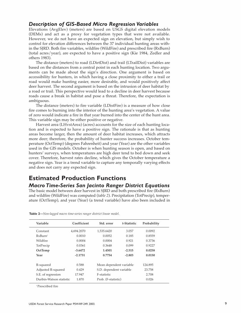
Estimated Production FunctionsMacro Time-Series San Jacinto Ranger District EquationsThe basic model between deer harvest in SJRD and both prescribed fire (RxBurn)and wildfire (WildFire) was computed (table 2). Precipitation (TotPrecip), temper-ature (OctTemp), and year (Year) (a trend variable) have also been included in


Table 2—Non-lagged macro time-series ranger district linear model.

Variable Coefficient Std. error t-Statistic Probability

Constant 4,694.2070 1,535.6420 3.057 0.0092RxBurn1 0.0010 0.0052 0.185 0.8559Wildfire 0.0004 0.0004 0.921 0.3736TotPrecip 0.0361 0.3648 0.099 0.9227OctTemp -3.6472 1.4501 -2.515 0.0258Year -2.1731 0.7754 -2.803 0.0150

R-squared 0.588 Mean dependent variable 124.895Adjusted R-squared 0.429 S.D. dependent variable 23.758S.E. of regression 17.947 F-statistic 2.708Durbin-Watson statistic 1.870 Prob. (F-statistic) 0.0261 Prescribed fire

the equation. In this linear equation there appears to be no strong statistical sig-nificance between the dependent variable and either type of fire. The coefficienton prescribed fire is 0.0009 and has a 0.18 t-statistic, indicating this variable hasminimal effect on deer harvest and is insignificant. Wildfire is very similar to theprescribed fire variable: the coefficient is 0.0004 and the t-statistic is 0.92, bothinsignificant and insubstantial. The only significant variables are October tem-perature and year.

October temperature is negative and has a significant t-statistic of 2.5. Thissign is consistent with hunter surveys indicating that when the temperature ishigh, the deer harvest goes down because deer are bedded to avoid the heat.Year has a 2.8 t-statistic and a negative coefficient of 2.17. This would indicatethat some systematic trend does exist within the data set. Possibly this variableis capturing other influences contributing to the decline in deer population with-in the SJRD. Total precipitation was expected to have a strong positive effect onvegetation growth and forage availability for deer; however, it does not show upas being significant. The R-squared value for this model is 0.58, and adjusted R-squared is 0.42. These values indicate some ability to explain the effects of fire ondeer harvest, as about half the variation in deer harvest is explained by “year”and “October” temperature. At this scale and with untransformed harvest andfire variables, there is no indication that the fire variables are related to variationin deer harvest.

A 1-year lag-on-acres-burned model was estimated to determine if the yearafter a fire allows for an increase in deer harvest. This lag is based on the expec-tation that new vegetation growth occurs in the year after a fire. Previousliterature found that the number of deer occupying burned stands of chaparralquadrupled the first growing season after the burn (Klinger and others 1989).However, a 1-year lag did not make a difference in deer harvest using thismodel. The 1-year lagged value of prescribed fire (-0.0047) and wildfire (0.0003)were both insignificant, with t-statistics of –0.70 and 0.72 respectively. Octobertemperature and year are almost the same as the previous model without a lag.The R-squared values for this model were similar to the previous model, at 0.58and 0.42.

San Jacinto Ranger District Log-Log ModelTaking the log of the dependent variable and the log of the combined wildfireand prescribed burn variable (LTotFire) results in a statistically significant effect.The coefficient for total fire shows a small magnitude of 0.048, but it has a signif-icant t-statistic of 2.3 (table 3). This appears to be in line with a previous studywhere the density of deer increased after wildfire (Klinger and others 1989). The


Table 3—Macro time-series ranger district log-log model.


Constant 41.8087 11.0701 3.7767 0.002LTotFire 0.0487 0.0205 2.3719 0.033TotPrecip -0.0001 0.0026 -0.3666 0.719OctTemp -0.0270 0.0107 -2.5362 0.024Year -0.0179 0.0056 -3.1993 0.006

R-squared 0.677 Mean dependent variable 4.809Adj. R-squared 0.585 S.D. dependent variable 0.202S.E. of regression 0.130 F-statistic 6.343Durbin-Watson statistic 2.066 Prob. (F-statistic) 0.002

sign on this variable is positive, and the coefficient can be interpreted as elastic-ities by using the log-log form. Therefore, a 1 percent increase in acres burnedwill lead to a 0.048 percent increase in deer harvest. The other significant vari-ables are October temperature (OctTemp) and year (Year). Again, a negative signon the October coefficient relates to observations that an increase in temperatureresults in a decrease in the number of deer harvested. The year variable indicatesthat a systematic effect exists within the model. This model’s explanatory poweris better with an R-square value of 0.67. The Durbin-Watson statistic of 2.06 indi-cates that autocorrelation is not a problem.

The same model (table 2) was also estimated with a 1-year lag. The coeffi-cient on the log of total fire lagged 1 year was 0.01 and had a t-statistic of 0.44,which indicates the lag is insignificant. The R-squared value did not changefrom the previous model.

Summary of Micro Regressions Based on GIS AnalysisThree regression models were estimated by using GIS-derived data (tables 4, 5,6). Two of these regression models—count data and OLS—show prescribedburns had a statistically significant effect on deer harvest. The count datamodel based on total fires is used for calculating the marginal benefits of addi-tional burning on deer harvest in the next section because of its superiorexplanatory power.

Percent of Hunting Location Area Burned, Micro ModelThis model describes the relationship between deer harvest (dependent vari-able) in each of the 37 hunting locations as a function of average elevation(AvgElev), the distance to dirt roads (LDirtDist) and trails (LTrailDist), the per-centage of hunting area experiencing a prescribed fire (PctRxBurn) and wildfire(PctWildfire) in the time period considered and the size of each hunting location(LHuntArea), the temperature in October (OctTemp) of that year, and year (Year)(table 4). The significant variables with t-statistics over 2.0 are distance to trailsand dirt roads, the size of the harvest area, and temperature in October. Wildfiresfor year one—the year during which the fire occurred—have a t-statistic of 1.8,which is considered statistically significant at the 10 percent level. However, thecoefficient on the wildfire is negative (-1.6), which would indicate that firesdecrease the probability of harvesting a deer in that year. The rest of the wildfireand all of the prescribed fire variables for each hunting area are not considered significant for any of the years using this percent-burned method. According tothese fire variables across time, their insignificance demonstrates that differ-ences in deer harvest cannot be attributed to fire. In this model, the distance todirt roads, distance to the nearest trail, the size of a hunting area and the temper-ature statistically influence deer harvest in October. The R-squared value of 0.18and the adjusted R-squared value of 0.17 indicate this model has relatively lowexplanatory power of deer harvest (table 4).

Micro GIS-Based Equation Using Total Acres Burned The second count data model (table 5) presents a different specification by usingtwo separate fire variables: the log of total acres of prescribed fire in the individ-ual hunting area during the time period, and the log of total acres of wildfire inthe individual hunting area during the time period. This equation controls forthe different size of the individual hunting areas by including a hunting area(acres) size variable. Total acres of prescribed fire (LTotRxFires) are significantduring the year of the prescribed fire, and its significance declines over the next 3 years. During the first year, the prescribed fire coefficient is 0.044 with a t-sta-tistic of 2.4. Because this count data model logs the fire acreage variables, it isequivalent to a log-log model. As such, the 0.044 is the elasticity. Total acres ofwildfire (LTotWFires) were not significant for any of the years in this equation.


This model has more explanatory power of the effect of fire on deer harvestthan the previous model based on a percent burn of each harvest area. This totalarea count data model R-squared value of 0.25 and the adjusted R-square 0.24 isalmost 40 percent greater than the percent burn count data model.

Micro GIS-Based Equation Using OLS Log-Log Form ofHarvest Per AcreThis equation was used as an alternative method to account for the differentsizes of hunting location. Using OLS regression of deer harvest per acre as afunction of fire and the other variables provides a similar pattern of signs andsignificance as the total area count data equation. In this model, a double logform was also used, but the dependent variable acted as a control measure forthe size of each hunting location by dividing harvest in each hunting location bythe number of acres in each location. The results of this model (table 6) show thatprescribed burns (LTotRxFires) have a statistically significant effect on deer har-vest in the first year with a t-statistic of 2.25. During the years after the fire,prescribed burn areas become less significant, which corresponds to the previouscount data model. The only time wildfire has a significant impact is during the second year (LTotWFires(-2)) after the burn. The sign of the coefficient for wild-fire in the second year is negative and less than one, which would imply anegative effect on deer harvest in that year. Distance to dirt roads (LDirtDist) isalso significant, a t-statistic of 5.17 and a negative coefficient -0.013. This maymean that hunting locations further away from dirt roads have a lower probabil-ity of the occurrence of hunters harvesting a deer or possibly that many hunters


Table 4—Count data model based on GIS with percent burned with lags.


Constant 2.7350 13.2598 0.2063 0.837LAvgElev -0.1989 0.1337 -1.4872 0.137PctRxBurn 1.6726 1.5733 1.0631 0.288PctRxBurn (-1) 1.5721 1.5961 0.9850 0.325PctRxBurn (-2) 2.1253 1.4669 1.4488 0.147PctRxBurn (-3) -0.3572 1.7741 -0.2013 0.840PctWildfire -1.6569 0.8893 -1.8631 0.063PctWildfire (-1) -1.1365 0.8064 -1.4094 0.159PctWildfire (-2) -0.4622 0.7290 -0.6340 0.526PctWildfire (-3) -1.5480 0.8390 -1.8451 0.065LDirtDistance -0.2429 0.0386 -6.2893 0.000LTrailDistance 0.4096 0.0426 9.6125 0.000LFireDist 0.0426 0.0467 0.9118 0.362LHuntArea 0.9377 0.0882 10.6355 0.000OctTemp -0.0343 0.0147 -2.3412 0.019Year -0.0035 0.0065 -0.5416 0.588

Overdispersion parameter

Alpha:C(17) -0.1999 0.103823 -1.925655 0.054

R-squared 0.186 Mean dependent variable 1.759Adj. R-squared 0.170 S.D. dependent variable 2.611S.E. of regression 2.379 Avg. log likelihood -1.629Restr. log likelihood -1922.63 LR index (Pseudo-R2) 0.300

Table 5—Count data model based on GIS using total acres burned with lags.


Constant 62.9643 23.1158 2.7239 0.007LAvgElev -0.2373 0.1307 -1.8154 0.070LTotWFires 0.0107 0.0171 0.6249 0.532LTotWFires (-1) 0.0083 0.0170 0.4877 0.626LTotWFires (-2) -0.0277 0.0155 -1.7903 0.073LTotWFires (-3) -0.0247 0.0156 -1.5830 0.113LTotRxFires 0.0441 0.0179 2.4609 0.014LTotRxFires (-1) 0.0275 0.0270 1.0193 0.308LTotRxFires (-2) 0.0115 0.0222 0.5169 0.605LTotRxFires (-3) 0.0115 0.0187 0.6155 0.538LDirtDist -0.2338 0.0377 -6.1944 0.000LTrailDist 0.3952 0.0418 9.4633 0.000LFireDist 0.0727 0.0474 1.5335 0.125LHuntArea 0.9407 0.0870 10.8128 0.000OctTemp -0.0121 0.0168 -0.7179 0.473Year -0.0347 0.0118 -2.9535 0.003

Overdispersion parameter

Alpha:C (17) -0.281 0.1081 -2.598621 0.009

R-squared 0.257 Mean dependent variable 1.759Adjusted R-squared 0.242 S.D. dependent variable 2.611S.E. of regression 2.273 Avg. log likelihood -1.618Restr. log likelihood -1920.633 LR index (Pseudo-R2) 0.305

Table 6—Least squares deer harvest per acre using GIS data model with lags.


Constant 1.3418 1.5883 0.8448 0.398LAvgElev -0.0097 0.0093 -1.0461 0.296LTotWFires 0.0012 0.0012 0.9632 0.336LTotWFires (-1) 0.0005 0.0012 0.4293 0.668LTotWFires (-2) -0.0022 0.0011 -2.0862 0.037LTotWFires (-3) -0.0018 0.0011 -1.6276 0.104LTotRxFires 0.0026 0.0012 2.2548 0.024LTotRxFires (-1) 0.0021 0.0019 1.1349 0.257LTotRxFires (-2) 0.0013 0.0015 0.8620 0.389LTotRxFires (-3) 0.0012 0.0013 0.9262 0.355LDirtDist -0.0130 0.0025 -5.1748 0.000LTrailDist 0.0183 0.0022 8.2132 0.000LFireDist 0.0051 0.0032 1.6072 0.108LHuntArea -0.0087 0.0062 -1.4098 0.159LOctTemp -0.0504 0.0860 -0.5859 0.558Year -0.0028 0.0008 -3.4364 0.001

R-squared 0.139 Mean dependent variable -4.533Adjusted R-squared 0.123 S.D. dependent variable 0.093S.E. of regression 0.087 F-statistic 8.684


do not venture very far from roads. This lower probability may be due to poach-ing along roads and/or to lower deer populations as a result of roadsfragmenting habitat. The positive coefficient on the distance to trails variable(LTrailDist) implies that having a distant proximity to trails increases the prob-ability of a deer harvest. All the other variables in this model fail to be significantindicators of deer harvest, except for the trend variable, year. Therefore, someunidentifiable systematic temporal change is occurring within the model.Overall, this model has a lower level of explanatory power than the total areamicro count data model. The R-squared value by using OLS is 0.13 and theadjusted R-squared value is 0.12 compared to twice this level of explanatorypower in the total area count data model (table 5).

Applying the Regression Production Functions To calculate the incremental effects of different levels of prescribed burning ondeer harvest, the acres-burned variable is increased from one level to a higherlevel in the regression model. We used the double-log macro time-series model(table 2) and the micro GIS-based double-log count data models (table 5), as thesetwo models have the highest explanatory power. The resulting predicted changein deer harvest will be valued in dollar terms.

Applying Results of Macro Time-Series ProductionFunction ModelThe double log Macro Time Series Production Function Model (table 3) is used toestimate the change in deer harvest. This model has a high explanatory powergiven that it explains almost 68 percent of the variation in deer harvest. As willbe recalled in this model, the lag effect proved insignificant. Therefore, the pre-scribed burning component of the total fire variable in this model is increased tothree different levels (1100, 4810, and 8510 acres, respectively) and the predictedlog of deer harvest is calculated at the mean of the other variables. The anti-logof harvest is then calculated to provide the estimate of the deer harvest withthat level of prescribed burning (table 7).

Applying Results of Micro GIS Production Function ModelThe results of both the count data model (table 5) and the least squares model (table 6) pro-vide positive evidence on the desirable effects of prescribed burning programs on deerharvest. Because the count data model has nearly double the R-squared value of the leastsquares model, the economic implications from prescribed burn programs will beevaluated by using the prescribed burn coefficients (table 5), the GIS count datamodel. By using this model it is possible to calculate the additional harvest fromadditional prescribed burn acres on deer harvest. In table 7, the first row forecaststhe estimated number of deer that would be harvested if only one acre of landwould burn. By using the current mean number of acres burned in each individ-ual hunting location for the GIS micro model (table 5), 30 acres, and thenmultiplying this by the total number of individual hunting locations, 37, a SJRD-wide deer harvest level is calculated. The forecast feature in the statisticalsoftware package EViews (Quantitative Micro Software 1997) does this. Theother variables are set at their mean levels. In the GIS micro model the effect offurther increasing prescribed burning is then calculated by increasing the num-ber of acres burned in each hunting location by 100 acres and then 200 acres toprovide a wide range of prescribed burning levels in the SJRD. The first level(1,100 acres) is about the average acres of prescribed burning over the last 20years in the SJRD. Maintaining this level of prescribed burning does provide anincrease in deer harvest over the no burning level. However, the gain in deerharvest increases more slowly with additional increases in burning in each huntarea (table 7).

14 USDA Forest Service Research Paper PSW-RP-249. 2003.

Table 7—Comparison of deer harvest response to prescribed burning using the macro time- series modeland GIS micro model.

Macro time-series model GIS micro model

1 NA 83 NA 1 42 NA1,100 1,100 116 33±3.99 2 1,100 58 16±4.454,810 3,710 124 8±3.99 3,710 66 8±4.458,510 3,700 128 4±3.99 3,700 71 5±4.45

1Although the variable Total Acres Burned reflects the combined prescribed acres and wildfire acres,for this simulation only, the prescribed burn acres are being changed because prescribed burned isthe management variable. 2 Because the dependent variable is the log of deer harvested, the 95 percent confidence interval wascomputed taking the antilog of the S.E. of the regression (0.13) (table 3) and multiplying it by 1.96(antilog 0.13 = -2.04 x 1.96 = ± 3.99).

The results suggest there is a substantial gain in deer harvest with the first1,100 acres burned (table 7), especially as calculated from the macro time-seriesmodel. However, a very similar diminishing marginal effect is evident fromboth the macro time-series production function regression and the micro GISproduction function regression after burning more than 1,100 acres. In otherwords, regardless of the spatial level of detail adopted, burning an additional3,710 acres is expected to result in about eight more harvested deer in the SJRD.

To determine the economic efficiency of additional prescribed burning, it isnecessary to compare the benefits of additional prescribed burning in the formof the economic value of deer harvest against the costs.

Valuation of Deer HuntingIn the SJRD the deer hunting regulation allows for a 1-month hunting seasonand a one-deer bag limit. According to CDFG, deer hunting is considered one ofthe major outdoor recreation activities in SJRD every year. Deer hunting hasoffered opportunities for recreational enjoyment as well as produced economicbenefits to the town of Idyllwild, California. Previous research on deer huntingin California showed that increased success rates and opportunities to har-vest a trophy deer (Creel and Loomis 1992) increase the economic value ofdeer hunting.

Linking hunter trips and success to economic values will result in a bio-economic relationship that ties fire management decisions to economics. Thus,we estimated the economic value of the additional deer harvest resulting fromthe prescribed burning program in the SJRD. By using both the travel costmethod (TCM) and the contingent valuation method (CVM) we can comparethe estimates of the change in consumer surplus for harvesting another deer inthe SJRD. This economic information will be useful to future policy decisionsregarding funding and implementation of a prescribed burning program.

Valuation MethodologiesContingent Valuation MethodCVM uses simulated (hypothetical) markets to quantify monetary values simi-lar to actual markets (Loomis and Walsh 1997). The method uses surveyquestions to elicit people’s net economic value or consumer surplus for an

15USDA Forest Service Research Paper PSW-RP-249. 2003.

Total acres1

burnedAdditional

acres burnedNo. deer

harvestedMarginal

increase indeer harvested

Prescribedacres

burned

No. deerharvested

Marginalincrease in

deer harvested

improvement in environmental or site quality by asking what additional amountthey would pay for a specified improvement. Thus, the method aims at elicitingpeople’s willingness-to-pay (WTP) in dollar amounts. In our application, CVMpresents hunters with a hypothetical market in which they can pay higher tripcosts to receive an increase in deer harvest opportunities. For simplicity in sur-vey design and administration, an open-ended WTP question was asked. Inaddition, the accumulated evidence to date is that the open-ended formats tendto produce conservative WTP estimates relative to dichotomous choice (Schulzeand others 1996). Although open-ended questions are more difficult to answerthan dichotomous-choice questions, hunters who have completed the deer-hunt-ing season at this area are quite familiar with the goods (deer) they are asked tovalue. Therefore, we felt this simplification was acceptable. The basic improve-ment being valued is the deer hunter’s consumer surplus per trip for aguaranteed deer harvest during the season, which is the difference between peo-ple’s maximum WTP per trip with guaranteed deer harvest (i.e., 100 percentchance of harvesting a deer) and people’s current maximum WTP per deer hunt-ing trip (i.e., deer hunting demand with around 9 percent deer harvest successrate).

The CVM model is specified as (equation 6):

[6] MWTPDeer = MaxWTPKill – MaxWTPCur

In which MWTPDeer is the change in hunter’s WTP for increasing deer har-vest rate, MaxWTPKill is the maximum WTP per trip with certainty of deerharvest, and MaxWTPCur is the current maximum WTP per trip.

Travel Cost MethodThe TCM has been a primary indirect approach for valuing environmentalresources associated with recreation activity over the last several decades.Clawson (1959) was the first to empirically estimate benefits using a travel-costframework. The basic concept of TCM is that travel cost (i.e., transportationcost, travel time) to the site is used as the proxy for the price of access to the site.When recreationists are surveyed and asked questions about the number of tripsthey take and their travel cost to the site, enough information can be generatedto estimate a demand curve. From the demand curve, net WTP or consumersurplus can be calculated. The explanatory variables that are often included intravel cost demand curves include age, income, family size, educational level,and other socioeconomic variables (Kahn 1995). Since we are interested in thebenefits of improvements at just one site with no changes at other sites, a single site TCM demand model will suffice for empirical analyses, and more complexmulti-site models such as hedonic TCM (Hybrid hedonic travel cost methoddeveloped by Brown and Mendelsohn 1984) or multinomial logit models(Sometimes called Random Utility Models [RUMs]) are more costly and complexthan warranted.

Definitions of TCM Price VariableBesides variable travel cost or its proxy, travel distance, many articles discuss theinclusion of a travel time variable in the demand function. Knetsch (1963) wasthe first to point out the opportunity cost of time is part of travel costs as well.Cesario (1976) suggested one-fourth the wage rate as an appropriate estimate ofthe opportunity cost of time based on commuting studies. For individuals withfixed workweeks, recreation takes place on weekends or during pre-designatedannual vacation and cannot be traded for leisure at the margin. In such cases,Bockstael and others (1987), Shaw (1992), and Shaw and Feather (1999) suggestthe opportunity cost of time no longer need be related to the wage rate. These


studies suggest that both the travel cost and travel time be included as separatevariables, along with their respective constraints—income and total time avail-able for recreation.

This study chooses its variables according to the consumer demand theoryand past literature (table 8). For instance, private hunting land serves as a substi-tute (or complement) for public hunting land in SJRD. Hunters were not askedthe distance to substitute sites nor to identify if there was a substitute site for theSJRD deer hunting. Because there are two other deer hunting areas in southernCalifornia that could be substitutes, our TCM estimates of consumer surplusmay overstate hunter’s net WTP for the SJRD by a slight amount. Hunters whohunt on opening day, belong to hunting organizations, hunted in previous sea-sons, and had a successful deer harvest may take potentially more hunting tripsbecause such hunters have higher preferences, experience, or skill in deer hunt-ing recreation. Because a majority of hunters in our dataset work a fixedworkweek, we assume the deer hunters maximize utility level subject to theirincome and time constraints (Shaw 1992). In other words, time is a constraintlike income for time intensive activities like hunting. Total time budget is con-structed for the TCM model according to the demographic time information.

For example, for a person who took a paid vacation to hunt, his/her totaltime budget (days) is obtained by 8 weekend days during the month of the hunt-ing season plus the number of weeks of paid vacation of the individualmultiplied by 5 days per week, for up to a maximum total of 30 days, which isthe length of the hunting season. For a person who took unpaid vacation time orreduced work hours to hunt, his/her total time budget is 16 days. For thosewho work their usual amount and hunt when they can, their total time budgetis 8 days, the number of weekend days during the October hunting season.Furthermore, for those unemployed and retirees, their total time budget is 31days. In this study, the total time budget ranges from 8 to 31 days, since thedeer-hunting season in SJRD lasted for 1 month only.

Table 8—Variables included in Regression Models and their Definitions.

Variable Definition

Dependent: NUMTRIPS Number of primary purpose of deer hunting trips taken to

the SJRD during 1999 deer hunting season.Independent: Age Hunter’s ageDeerKill Did you harvest a deer in this area during this hunting season?

1= YES, 0 = NOHuntOpen Did you hunt on opening day of the D-19 season?

1= YES, 0 = NOHuntOrg Are you a member of a Sportsman’s organization?

1= YES, 0 = NOPrevSeas Have you hunted in this area in a previous season?

1= YES, 0 = NOPrivLand Did you hunt on private land?

1= YES, 0 = NORTravMiles Round-trip travel miles from home to the hunt locationPcInc Hunter incomeToTimeBud Total time budget. TravTime Number of hours one-way travel time


Count Data Nature of TCM Dependent VariableThe non-negative integer characteristic in every observation for the dependentvariable (i.e., NUMTRIPS) is the so-called “count data.” Given the count dataform of the dependent variable, a preferred estimation model should be able tocontrol for integer nature of the dependent variable (Creel and Loomis 1990). Inthis study, the negative binomial count model was used to estimate the demandfunction. The negative binomial is the more generalized form of the Poisson dis-tribution, which allows the mean of trips to be different from its variance. Thenegative binomial and Poisson count data models are equivalent to a semi-log ofthe dependent variable functional form.

The count data TCM model is specified in equation 7:

[7] NUMTRIPS = EXP (C(1) + C(2) x Age + C(3) x DeerKill + C(4) xHuntOpen + C(5) x HuntOrg + C(6) x PrevSeas +C(7) x PrivLand - C(8) x RTravMiles + C(9) x PcInc + C(10) x ToTimeBud - C(11) x TravTime)

In equation 7, we expected the coefficient for DeerKill [C(3)] to have a posi-tive sign, since hunters would likely take more hunting trips if the huntingquality had been good. Also, if hunters hunted on the opening day [C(4)], privateland [C(7)], and/or previous seasons [C(6)] and belong to hunting organizations[C(5)], then we expected a positive effect on the number of trips the hunter took,as these variables indicated a strong preference for the deer hunting activity. Forthose hunters with a higher income level [C(9)] and/or higher total time budg-et [C(10)], we expected more hunting trips as well, as a result of less bindingincome and time constraints. However, round-trip travel distance [C(8)] andtravel time [C(11)] are expected to have negative effects on the number of hunt-ing trips because increases of these two variables increase hunter’s expense.

Calculation of Consumer Surplus in TCM The consumer surplus from deer hunting is computed from the demand curve asthe difference between people’s WTP (e.g., the entire area under the demandcurve) and what they actually pay (e.g., their travel costs). Because the countdata model is equivalent to a semi-log functional form, consumer surplus froma trip is calculated as the reciprocal of the coefficient on round-trip travel milestimes the average cost per mile, expressed in RTravMiles x $0.30/mile (see equa-tion 9) (Sorg and others 1985).

CVM and TCM ComparisonsLiteratures in CVM and TCM comparisons have usually just compared the averageconsumer surplus for existing conditions. For example, Carson and others (1996)found in their study that on average, CVM-derived values were usually smallerthan revealed preference estimates like TCM. To test the consistency between twononmarket good valuation methods, we compared the CVM and TCM in thisstudy for the improvement in deer hunting quality due to the prescribed burningprogram. A Tobit model was used for the analysis of open-ended WTP responsesfrom CVM because our open-ended dependent variable only has a single bound at0. The Tobit model uses the open-ended WTP response as the dependent variablein CVM (i.e., people’s current WTP), and the independent variables similar toTCM. The same variables are used because both methods are trying to explainconsumer surplus. For TCM, this is done via the demand curve. Meanwhile, forCVM, it may be thought of as the inverse demand function.


The CVM Tobit model is equation 8:

[8] MaxWTPCur = C(1) + C(2) x Age + C(3) x DeerKill + C(4) x HuntOpen + C(5) x HuntOrg + C(6) x PrevSeas + C(7) x PrivLand - C(8) x RTravMiles + C(9) x PcInc + C(10) x ToTimeBud - C(11) x TravTime

For the same reasons as in the TCM equation, we expected round-triptravel miles and travel time to hold negative signs in equation 8.

Data for TCM and CVM ModelsFor cost effectiveness in data collection, a mail questionnaire was used. Therewere six sections along with one demographic section. The first section gave abrief introduction of the questionnaire and then asked about the number ofhunting trips taken this season to the SJRD and prior hunting experiences inthe SJRD. The second section gathered information on the land ownership of thearea hunted, weapon type used, and information on deer harvest characteristicsif the hunter had been successful. The third section asked about the hunter’sinvolvement in opening day of the hunting season. Section four inquired aboutthe travel distance and travel time to the hunting area. The fifth section askedquestions about the hunter’s expenses as well as the hunter’s WTP higher tripcosts for the hunting experience on the most recent trip. Specifically, hunterswere asked an open-ended question pertaining to the maximum increase in deerhunting expenses before they would not have taken this trip. Also, the CVManalysis was used to measure hunter increases in WTP associated with increas-ing deer harvest success, including a 100 percent chance of harvesting a deerduring the season. Our WTP estimate from CVM is compensating variation,rather than consumer surplus, but the two measures are nearly identical in mostapplications since the income effect is quite small for deer hunting. The sixth sec-tion asked about the characteristics of the hunter’s preferred hunting area. Thefinal section of the survey detailed demographic information such as age,income, family size, educational level, and other socioeconomic variables fromthe respondents.

Survey Mailing and Response RateDuring the 1999 deer hunting season, a mail questionnaire (appendix I) was sentto a random sample of deer hunters with licenses for deer in Zone D19, whichincludes the SJRD. Of 762 questionnaires mailed to deer hunters in Californiaduring the 1999 hunting season, 7 were undeliverable. A total of 356 deerhunters’ responses were collected after two mailings. Response rate is, there-fore, approximately 47 percent. Among these respondents, 69 did not hunt deerin the San Bernardino National Forest, SJRD.

Descriptive StatisticsMore than 72 percent of respondents did hunt on opening day. The average deerhunter is around 43 years old, with a mean income slightly more than $33,000dollars (table 9).


The distribution of dependent variable observations reflects how manyhunting trips the hunter took during the 1999 deer-hunting season:

Number of trips Number of deer hunters

NA 580 21-5 207

6-10 5311-15 1316-20 1021-30 631-40 041-50 1

Above 50 1Total 351

The majority of deer hunters took at least one hunting trip during the sea-son. Two hunters indicate they did not take any hunting trip in the 1999deer-hunting season. Fifty-eight hunters did not answer this question becausethey did not hunt within the SJRD. In addition more than 70 hunters took morethan 6 hunting trips in the 1999 deer-hunting season. One reasonable explana-tion for this is that those deer hunters live close by the SJRD.

Statistical Results of TCM and CVM ValuationModelsTravel Cost MethodA negative binomial count data model was used to estimate the statistical rela-tionship between number of trips and all the independent variables (table 10).There is a negative effect of travel miles (RTravMiles), travel time (TravTime),and income (PcInc): increase in travel distance and time results in a decrease inthe number of trips the hunter will take. The negative coefficient explains the


Table 9—Statistical information of TCM variables.

Variable1 Mean Median Maximum Minimum Std. Deviation

NUMTRIPS 5.56 4.0 62.0 1.0 6.26Age 43.0 42.0 80.0 13.0 13.40PctDeerKill 9.7 0.0 NA NA 0.29HuntOpen (Pct) 72.3 NA NA NA 0.45HuntOrg (Pct) 35.0 NA NA NA 0.48PrevSeas (Pct) 81.3 NA NA NA 0.39PrivLand (Pct) 15.0 NA NA NA 0.36RTravMiles 103.80 80.0 800.0 0.5 95.11PcInc $33,148.00 $32,500.00 $100,000.00 $833.00 $18,287.00ToTimeBudget 19.78 23.0 31.0 0.0 10.27TravTime 1.43 1.2 9.0 0.10 0.98

1 See table 8 for definition of variables

disutility effect caused by travel time and travel cost increases. Income, in thisstudy, is insignificant. Also, regression results of this study indicate whether ahunter successfully harvested a deer during the hunting season (i.e., DeerKill),whether the individual hunted on opening day (i.e., HuntOpen), whether thehunter hunted in this area in a previous season (i.e., PrevSeas), and whether totaltime budget (i.e., ToTimeBud) had significant effects on the number of huntingtrips hunters took. Indeed, hunters who hunted the opening day hunted in thisarea last year, harvested a deer, had a larger time budget, and took more huntingtrips. Consistent with economic theory, hunters with longer round-trip travelmiles (RTravMiles) and travel time (TravTime) tended to take fewer hunting trips.

The consumer surplus is calculated by using Sorg and others’ (1985)method (equation 9) in which the $0.30 is the 30 cents per mile sample aver-age cost per mile.

[9] Consumer Surplus = 1/β (i.e. coefficient of distance) x $0.30/mile (i.e. cost per mile) = 1/0.002230 x $0.30

= 448.43 x $0.30 = $134.53/trip

Finally, the 90 percent confidence interval (table 10) is obtained by equation 10:

[10] 90 percent confidence interval on Consumer Surplus per Trip = 1/(βDIST ± 1.64 x 0.000895) x $0.30/mile = $81.13 - $393.59 per trip

Estimating the Benefits of Harvesting an Additional DeerThe average number of trips per hunter is 5.56 trips, and 1 out of 10 deer hunterssuccessfully harvests a deer. Therefore, average consumer surplus per deer har-vested is 10 x 5.56 x 134.53 = $7,480 per deer harvested. To calculate theincremental or marginal value of an additional deer suitable to compare to mar-ginal costs, we can use the TCM demand equation to predict the extra number of trips deer hunters would take if they knew they would harvest a deer that sea-son. This essentially shifts the demand curve out by the amount of the coefficient


Table 10—Estimated negative binomial count data TCM demand equation.

Variable1 Coefficient Std. Error Z-Stats Probability

Constant 1.325 0.216 6.123 0.00Age 0.001 0.004 0.369 0.71DeerKill 0.367 0.155 2.370 0.02HuntOpen 0.524 0.115 4.564 0.00HuntOrg 0.068 0.106 0.639 0.52PrevSeas 0.285 0.135 2.122 0.03PrivLand 0.038 0.132 0.289 0.77RTravMiles -0.002 0.0009 -2.490 0.01PcInc -1.00E-06 2.78E-06 -0.360 0.72ToTimeBud 0.010 0.005 2.099 0.04TravTime -0.289 0.087 -3.334 0.00

R2 = 0.21, Adjusted R2 = 0.17

Consumer surplus = $134.53/trip 90 Pct confidence interval: $81.13 - 393.60Marginal consumer surplus per deer harvested = $257.17/deer 90 Pct confidence interval: $155 - $752


on deer harvest. The equation predicts that each hunter would take 1.9116 moretrips each season if hunters knew they would harvest a deer. Therefore, the mar-ginal value of another deer harvested (i.e., marginal consumer surplus) is equalto $134.53 x 1.9116 = $257.17 per deer harvested. Finally, the 90 percent confi-dence interval (CI) in table 10 for an additional deer harvested is obtained byapplying the 90 percent CI on the value per trip times the additional number oftrips taken by the hunter:

[11] 90 percent confidence interval of the value of harvesting an additional deer = 1.9116 x $81.13 - 1.9116 x 393.59 = $155 - $752

per deer harvested.

Contingent Valuation MethodIn the survey, people were asked their maximum WTP for their most recent tripunder current conditions, and their maximum WTP per trip for a 100 percentguaranteed chance to harvest a deer over the season. The consumer surplus andpeople’s maximum WTP per trip were computed (table 11). The CVM estimate ofconsumer surplus under current low success rate (9 percent) conditions was$17.59 per trip, while with 100 percent chance of harvesting a deer over the sea-son the consumer surplus estimate rose to $116.19 per trip. The per trip figurerequires multiplying by the change in number of trips over the season to allowcomparison with TCM, since TCM indicates a change of 1.9116 trips when deerharvest is certain over the season. In CVM, therefore, consumer surplus is equalto MaxWTPKill (at the mean) multiplied by 1.9116 trips, or $222/deer.

Table 11—CVM results (dollars per trip). 1

MaxWTPKill MaxWTPCur MWTPDeer

Mean 116.19 17.59 98.60Median 50.00 0.00 50.00Maximum 2300.00 500.00 2300.00Minimum 0.00 0.00 0.00Std. dev. 200.24 58.68 191.99

Marginal consumer surplus per deer harvested = $222/deer, 90 Pct confidence interval: $178 - $265

1 See table 8 for definition of variablesThe 90 percent Confidence Interval (C.I.) on seasonal consumer surplus for

harvesting an additional deer is:

[12] 90 pct C.I. = DTrips x Mean ± (t-value@90Pct) x ((St. Dev.) /√n)= 1.9116 x [$116.19 ± 1.64 x (200.2411/√210)]= $178 - $265 per deer harvested,

in which D is the change in number of trips when deer harvest is certain.

Comparing the Consumer Surplus from TCM and CVMThe marginal consumer surplus of harvesting an additional deer estimated byTCM is $257 (table 10), and the marginal consumer surplus estimated by CVM is$222 a deer (table 11). Comparing the 90 percent confidence intervals, TCM has arange from $154 to $752, and CVM ranges from $178 to $265 per deer harvested.

Table 12—CVM inverse demand curve.

Variable1 Coefficient Std. Error Z-Stats Probability

Constant -143.8908 66.9346 -2.1497 0.032Age -0.0958 1.0850 -0.0883 0.930DeerKill 123.0983 42.4801 2.8978 0.004HuntOpen 15.4554 32.3074 0.4784 0.632HuntOrg 34.3721 29.8438 1.1517 0.249PrevSeas -44.9252 35.8284 -1.2539 0.210Privland -19.1205 39.4412 -0.4848 0.628RTravMiles 0.3784 0.2262 1.6727 0.094PcInc 0.0004 0.0008 0.5516 0.581ToTimeBud 0.7401 1.4302 0.5175 0.605TravTime -27.7475 24.8721 -1.1156 0.265

Marginal value per deer harvest = 1.9116 trips x 123.0983 = $235/deer1 See table 8 for definition of variables

To estimate the CVM inverse demand curve, 246 observations were usedafter 103 observations were dropped due to one or more missing variables. Theresults (table 12) show consistency between the CVM inverse demand functionand the TCM demand function for most independent variables except whetherthe hunter had hunted in this area in a previous season (i.e., PrevSeas), whetherthe hunter had hunted on private land (i.e., Privland), and round-trip travel milesfrom home to the hunt location (i.e., RTravMiles). Specifically, the remainingseven variables were either the same sign or insignificant in both TCM andCVM. The comparison results indicate that the variable “whether the huntersuccessfully harvested a deer” (i.e., DeerKill) plays a vital role in influencingpeople’s current WTP (i.e., MaxWTPCur) for deer hunting in the SJRD—similarto the TCM demand function. The coefficient on whether the hunter harvested adeer (i.e., DeerKill) (table 12) offers a second CVM way to calculate the margin-al value per deer harvest per hunter. By multiplying $123/deer/trip with 1.911trips, marginal value per deer harvest is $235/deer. This value is still consistentwith previous TCM and CVM analysis in tables 10 and 11.

Applications of Values to Estimate Benefits ofPrescribed BurningBoth CVM and TCM were used to evaluate the change in deer hunting benefitsdue to an increase in deer harvest resulting from additional prescribed burning.In the TCM analysis, we found the change in consumer surplus is $257 withadditional trips the hunter took in response to increasing deer harvest. FromCVM, we found the change in consumer surplus is slightly less than the TCMresult: $222 per deer harvested. The mid-point marginal consumer surplus ofTCM and CVM, therefore, is $239.5 per deer harvested, or $240 with rounding.

The annual deer hunting benefit of additional acres of prescribed burningwas computed (table 13). While the initial deer hunting benefit response to pre-scribed burning of 1,100 acres ranges from $3,840 to $7,920 depending on themodel, the incremental gain for more than the current acreage of prescribedburning is quite similar across models. In other words, the annual economichunting benefit of increasing prescribed burning from its current level of 1,100acres to 4,810 acres is $1,920, regardless of the model used. Likewise for an addi-


tional 3,700 acres of prescribed burning, to 8,510 acres, the deer hunting benefitis between $960 and $1,200 each year, which is fairly similar despite the differ-ent modeling approaches. Table 13 Annual deer hunting benefits from increased prescribed burning: macro time-series model and GISmicro model results.

Macro time-series model GIS micro model

NA NA NA NA NA NA1,100 33 $7,920 1,100 16 $3,8403,710 8 $1,920 3,710 8 $1,9203,700 4 $960 3,700 5 $1,200

Comparison to CostsThe costs of prescribed burning on the San Bernardino National Forest rangefrom $210 to $240 per acre (Walker 2001). This is a much lower total cost per acrethan reported by González-Cabán and McKetta (1986) but substantially higherthan the direct costs per acre for southwestern National Forests reported inWood (1988). Nonetheless, if we use the $210 per acre figure, the full incre-mental costs of burning the first 1,100 acres would be $231,000, with eachadditional 3,710 acres burned costing $779,100. The deer hunting benefits rep-resent, at most, about 3.4 percent of the total costs of the first 1,100 acres ofprescribed burning.

This finding can be used in two ways. First, the incremental costs of includ-ing deer objectives in the prescribed burn should not exceed $8,000, as theincremental benefits are no larger than this. Second, the other multiple use ben-efits such as watershed and recreation as well as hazardous fuel reductionbenefits to adjacent communities would need to make up the difference if theprescribed burning program is to pass a benefit-cost test. If prescribed burningof 1,100 acres prevented as few as two residential structures from burning, theprescribed burn program would likely pass a benefit-cost test. Such an assess-ment is beyond the scope of this study, however. Many of these multiple usebenefits from a prescribed fire are received for at least 5 years and as many as 10-12 years (Gibbs and others 1995). Thus, a simple annualization of the costsbrings the 1,100-acre figure down to $23,100. Deer hunting benefits would coverbetween 16 and 34 percent of the annual costs of the first 1,100 acres. However,deer hunting benefits would only be minimal (less than 1 percent) compared tofurther increases in prescribed burning.

ConclusionThis study evaluated the response of deer harvest and deer hunting benefits toprescribed burning in the SJRD of California. To estimate hunters’ benefits orWTP for harvesting an additional deer, the individual observation TCM andopen-ended CVM were used. The mean WTP to harvest another deer is about$257 for TCM and $222 for CVM. One reason for such consistency may be due tothe respondents’ hunting in the SJRD in previous years. About 80 percent of thedeer hunters in SJRD hunted there in the previous season. Also, the changes intrips for the increase in harvest estimated from TCM were used to scale up both TCM and CVM per trip benefits to get a seasonal change. Because TCM containsno hypothetical bias and the TCM result is consistent with the CVM estimate, itmay be that the hypothetical bias in this study was minimal for CVM.


Additionalacres

burned

Marginal increase in

deer harvest

Annual increasein deer hunting

benefits

Additionalprescribed

acres burned

Marginalincrease in

deer harvest

Annual increasein deer hunting

benefits

With regard to the response of deer harvest to prescribed fire and wildfire,we compared a macro level, time-series model that treated the entire SJRD as onearea and a micro GIS model that disaggregated the SJRD into the 37 huntinglocations reported by hunters. Both models gave somewhat mixed results in thatsome statistical specifications showed no statistically significant effect of pre-scribed burning and/or a negative effect of lagged wildfire. However, the betterfitting (68 percent of variation explained) log-log model functional form of themacro time-series model did show a statistically significant effect of the com-bined prescribed fire and wildfire acres on deer harvest over the 20-year periodof 1979-1998. Two of the three micro GIS model specifications indicate that theinitial effect of prescribed burning had a statistically significant effect on deerharvest in the 37 hunting locations within the SJRD. Lagged effects of prescribedburning were consistently insignificant in our models, suggesting that most ofthe benefits occur in the year of the burn. The macro time-series model estimat-ed a larger response to burning of the first 1,100 acres than the micro GIS modeldid, but for increases in fire beyond 1,100 acres, the two models provided near-ly identical estimates.

Combining the average of the TCM and CVM estimated economic benefitswith the deer harvest response to fire yields annual economic benefits rangingfrom $3,840 to $7,920 for the first 1,100 acres burned. For 3,710 additional acresburned, the gain is $1,920 annually, while for an additional 3,700 acres theincrease ranges from $960 to $1,200 per year.

The costs of prescribed burning on the San Bernardino National Forest rangefrom $210 to $240 per acre. Thus, the costs to burn an additional 1,100 acres are$231,000, which is an order of magnitude larger than the deer hunting benefitsgained. Specifically, the deer hunting benefits of the first 1,100 acres representabout 3.4 percent of the total costs. Thus, the other multiple use benefits of pre-scribed burning, such as providing opportunities for dispersed recreation,protecting watershed, and reducing hazardous fuel in surrounding communi-ties, would have to cover the rest. Investigating the extent of these benefitswould be a logical next step in evaluating the economic efficiency of prescribedburning in the SJRD.

Although fire management practices have been identified as having wide-spread impacts on deer habitats, many other factors that affect deer habitat exist.These other factors include livestock grazing, timber harvesting, urban develop-ment, diseases, and habitat loss along with annual weather patterns (CDFG1998). This study attempted to take into account as many factors as possible.However, the amount of data and time available for modeling were a constraint.

The macro time-series model demonstrated positive and significant effectsfrom total fire when both wildfire and prescribed fire variables were combined.This appears to be in line with a previous study where the density of deerincreased the growing season after the burn (Klinger and others 1989). A studyof prescribed burning in northern California found prescribed burning to onlyhave modest effects of increasing deer habitat use and mentioned that anyincreases in use are difficult to quantify (Kie 1984).

Some future improvements in our modeling effort that may better isolate theeffects of prescribed burning on deer habitat include controlling for the severi-ty of wildfire because different fire severities will have different effects onvegetation and soils (Ryan and others 1983). Furthermore, including a vegetationand soils layer in the GIS model, rather than using elevation as a proxy, couldimprove the predictive ability of the GIS-based model as well.

Subject to these caveats, this paper has demonstrated two approaches toestimate a production function relating prescribed burning to effects on deerharvest. We found positive and significant effects on deer harvest for two of thethree GIS models and the positive impact of fire using a macro time-seriesmodel. The USDA Forest Service and CDFG can make use of these approachesfor future cost benefit analysis of prescribed burning.


References Bockstael, Nancy E.; Strand, Ivar E.; Hanemann, W. Michael. 1987. Time and the recreation demand

model. American Journal of Agricultural Economics 69 (May): 293- 302.Brown, Gardner; Mendelsohn, Robert. 1984. The hedonic travel cost method. Review of Economics

and Statistics 66: 427-433.California Department of Fish and Game. 1998. An assessment of mule and black-tailed deer habi-

tats and populations in California, with special emphasis on public lands administered by theBureau of Land Management and the United States Forest Service. Report to the CaliforniaFish and Game Commission; February 1998. Sacramento, CA: California Department of Fishand Game; 56 p.

Carson, Richard; Flores, Nicholas; Martin, Kerry; Wright, Jennifer. 1996. Contingent valuation andrevealed preference methodologies: comparing the estimates for quasi-public goods. LandEconomics 72 (1): 80-99.

Cesario, F. J. 1976. Value of time in recreation benefit studies. Land Economics 52(1): 32-41. Chou Yue-Hong. 1997. Exploring spatial analysis in geographic information systems. Santa Fe,

NM: OnWord Press; 474 p.Clawson, Marion. 1959. Methods for measuring the demand for and value of outdoor recreation.

Reprint no. 10, Washington, DC: Resources for the Future, Inc.Creel, M. D.; Loomis, J. 1990. Theoretical and empirical advantages of truncated count data estima-

tors for analysis of deer hunting in California. American Agricultural Economics Association(May): 434-441.

Creel, M. D.; Loomis, J. 1992. Modeling hunting demand in the presence of a bag limit with testsof alternative specifications. Journal of Environmental Economics and Management 22: 99-113.

Environmental Systems Research Institute, Inc. 1995. Understanding GIS, the ARC/INFO method.Redlands, CA: ESRI; 608 p.

Forsythe, Kenneth. 1999. Using conditional probabilities to evaluate animal and animal productimport requests: Part II—background and theory. Washington, DC: U.S. Department ofAgriculture, APHIS Technical Report; 149 p.

Gibbs, P.; Freeman, D.; Harvey, C.; Lawson, R.; Valenzuela, K.; Pumphrey, D. 1995. Area analysis andplan for prescribed burning. Idyllwild, CA: San Jacinto Ranger District, Forest Service, U.S.Department of Agriculture; 38 p.

González-Cabán, A. 1993. Improving the US Forest Service’s fire management planning systemcapabilities to use nonmarket values. Wildfire 2: 16-21.

González-Cabán, Armando; McKetta, Charles. 1986. Analyzing fuel treatment costs. WesternJournal of Applied Forestry 1(4): 116-121.

Hellerstein, Daniel. 1992. The treatment of nonparticipants in travel cost analysis and otherdemand models. Water Resources Research 28(8): 1999-2004.

Hesseln, Hayley. 2000. The economics of prescribed burning: A research review. Forest Science46(3): 322-334.

Kahn, James R. 1995. The economic approach to environmental and natural resources. Orlando, FL:Dryden Press; 536 p.

Kie, John G. 1984. Deer habitat use after prescribed burning in northern California. Res. NoteRN-PSW-369. Albany, CA: Pacific Southwest Forest and Range Experiment Station, ForestService, U.S. Department Agriculture; 3 p.

Klinger, Robert C.; Kutilek, Michael J.; Shellhammer, Howard S. 1989. Population responses ofblack-tailed deer to prescribed burning. Journal of Wildlife Management 53 (4) 1989: 863-870.

Knetsch, J.L. 1963. Outdoor recreation demand and benefit. Land Economics 39 (November): 387-396.

Loft, Eric R. 1998. Economic contribution of deer, pronghorn antelope and sage-grouse hunting tonortheastern California and implications to the overall “value” of wildlife. California WildlifeConservation Bulletin (11); 42 p.


Loomis, John B.; Updike, D.; Unkel, W. 1989. Consumptive and non-consumptive values of a gameanimal: The case of California deer. Transactions of the 54th North American Wildlife andNatural Resources Conference. Washington, DC: Wildlife Management Institute; 640-650.

Loomis, John B.; Walsh, Richard G. 1997. Recreation economic decisions: Comparing benefits andcosts. Second ed.; State College, PA: Venture Publishing, Inc.; 440 p.

Paulek, Tom. 1989. San Jacinto/Santa Rosa Mountains deer herd management plan. Sacramento,CA: California Department of Fish and Game. Technical Report; 66 p.

Quantitative Micro Software, LLC. 1997. Eviews 3.0 user's guide. Irvine, CA: Quantitative MicroSoftware, LLC; 692 p.

Ryan, Kevin C.; Noste, Nonan V. 1983. Evaluating prescribed fires. In: Lotan, James E., editor.Proceedings, symposium and workshop on wilderness fire; 1983 November 15-18. Gen. Tech.Rep. GTR-INT-182. Missoula, MT: Intermountain Forest and Range Experiment Station, ForestService, U.S. Department of Agriculture; 434 p.

Schulze, W.; McLelland, G.; Waldman, D.; Lazo, D. 1996. Sources of bias in contingent valuation. In:Bjornstad, D.; Kahn, J., eds. The contingent valuation of environmental resources:Methodological issues and research needs. Cheltham, UK: Edward Elgar; 97-116.

Shaw, W.D. 1992. Searching for the opportunity cost of an individual’s time. Land Economics 68(February): 107-15.

Shaw, W. Douglas; Feather, Peter. 1999. Possibilities for including the opportunity of time in recre-ation demand systems. Land Economics 75(4): 592-602.

Society of American Foresters. 1985. A question of values: Below-cost timber sales in the nationalforests. The 1985 report of the below-cost timber sales task force of the Society of AmericanForesters. Bethesda, MD: Society of American Foresters; 63 p.

Sorg, Cindy; Loomis, J.; Donnelly, Dennis M.; Peterson, George; Nelson, Louis J. 1985. Net economicvalue of cold and warm water fishing in Idaho. Resource Bulletin RM-RB-11. Fort Collins, CO:Rocky Mountain Forest and Range Experiment Station, Forest Service, U.S. DepartmentAgriculture; 66 p.

Walker, Norm. 2001. Prescribed fire costs. Email from Norm Walker, Division Chief, San JacintoRanger District to Lucas Bair, Colorado State University. January 26, 2001.

Wood, Donald B. 1988. Costs of prescribed burning in southwestern ponderosa pine. WesternJournal of Applied Forestry 3(4): 115-119.

Zedler, Paul H.; Gautier, Clayton R.; McMaster, Gregory S. 1983. Vegetation change in response toextreme events: The effect of a short interval between fires in California chaparral and coastalshrub. Ecology 64(4): 809-818.



Appendix 1. Survey instrument used in the study


Appendix 2. San Bernardino National Forest

The Forest Service, U.S. Department of Agriculture, is responsible for Federal leadershipin forestry. It carries out this role through four main activities:

• Protection and management of resources on 191 million acres of National ForestSystem lands;

• Cooperation with State and local governments, forest industries, and private land-owners to help protect and manage non-Federal forest and associated range andwatershed lands;

• Participation with other agencies in human resource and community assistance programs to improve living conditions in rural areas; and

• Research on all aspects of forestry, rangeland management, and forest resources utilization.

The Pacific Southwest Research Station• Represents the research branch of the Forest Service in California, Hawaii, American

Samoa, and the western Pacific.

The United States Department of Agriculture(USDA) prohibits discrimination in all its pro-grams and activities on the basis of race, color,national origin, gender, religion, age, disabili-ty, political beliefs, sexual orientation, andmarital or familial status. (Not all prohibitedbases apply to all programs.) Persons with dis-abilities who require alternative means forcommunication of program information(Braille, large print, audiotape, etc.) shouldcontact USDA’s TARGET Center at:

202-720-2600 (voice and TDD)

To file a complaint of discrimination, write:USDA DirectorOffice of Civil RightsRoom 326-WWhitten Building14th & Independence Avenue, SWWashington, DC 20250-9410

or call:(202) 720-5964 (voice or TDD)

USDA is an equal opportunity provider andemployer.

Federal Recycling Program Printed on Recycled Paper

United States

Departm

ent of A

gricultureForest Service

Pacific S

outhw

estR

esearch Statio

n

Research Paper

PSW-R

P-249

Eco

no

mic V

alue o

f Big G

ame H

abitat

Pro

du

ction

from

Natu

ral and

Prescrib

ed F

ire

of agriculture habitat production from - fs.fed.us · united states department of agriculture...

Documents