RD-RI68 169 LONG-TERN EFFECTS OF DREDGING OPERRTIONS PROORRM THE 1/1DUHANISH URTERNRY CA..(U) ARHY ENGINEER NATERUNYSEXPERIMENT STATION VICKSBURG HS ENVIR.. C L TRUITT

UNCLASSIFIED MRR 96 IES/TR/D-86-2 F/B 13/2 NL

moonsUUUhnhhUUlllE-llllllEEEmhmlhihml~Uln~n"EKEnunull~

., ~ ~ ~ ~ ~ ~ ~ ~ ~ ~ ~~~J U."'.-tW:- . .9."r1... a.. g. r t, -

'wry T - -4

i7

U.,.'

'W.2

4'.

-~~ Jc -

LONG-TERM EFFECTS OF DREDGINGOPERATIONS PROGRAM

1 ECANICAL RE PORT D-86-2

T-HE DUWAMISH WATERWAY CAPPINGDEMONSTRATION PROJECT: ENGINEERING

ANALYSIS AND RESULTS OF00 PHYSICAL MONITORING

Cp.,( L. Tr it

L iv i r il v y

PE PA H 1"11 N.! OF TH L /ARI 'Y~t t pewnt-\ r i t SOtion, (2 ~ of Fnqin( -

P , 1, Vick',)ro Missis ' pp 39180-06'31

3: ELE,'TE

MAY 2 8 986

Matrch 1986~A £ Final Report-

4-~ I ~ ' ' US Army Engineer District, Seattle

0 AZOSeattle, Washington 98124-2255

DEPARTMENT OF THE ARMY r.L~e :::,US Army Corps of Enginters

Washington, DC 20314-1000A

Ud.Work Unit 31774

86 5 27 08 7

0 ~ ~ ~ ~ ~ ~ ~ ~ w jcJ *1-*-0 . - .D1-at' - - - Pla' ,-f.4:jt

-OIPUa] leo s'.ejaeqp b aC)b ie I

JD alb~OPOL1a" O U0VOIUM pat Auabealu

suolvjad b~paj] tI s~;J3 iai-uoA

(waadUILCJOA pia9WsdA~e~ajv uolds JO jg PdbqJ~PLQ bu~iIenje

io1 soboioowav so1 ;,.O ~ JO p tai iAaabe"u

suo'ieied11b0,bpa i jo ~ so jO wia6uo

uo~~~~dns~ 0~t0lsoaiio6'pi

.swujboj 1~~~~~~~ buba j4S313IsuwaIu

a~jj;o uot~~t~nd spngu' poda ;oS~iJS-QO-V

UnclassifiedSECURITY CLASSIFICATION OF THIS PAGE (When De. Entered)

TDOCUMENTATION PAGE READ INSTRUCTIONSREPORT DBEFORE COMPLETING FORM

1. REPORT NUMBER 2. GOVT ACCESSION NO. 3. RECIPIENT'S CATALOG NUMBERTechnical Report D-86-2

4. TITLE (and Subt.t) S TYPE OF REPORT & PERIOD COVERED

THE DUWAMISH WATERWAY CAPPING DEMONSTRATION Final reportPROJECT: ENGINEERING ANALYSIS AND RESULTS

OF PHYSICAL MONITORING 6. PERFORMING ORG. REPORT NUMBER

7. AUTHOR(.) S. CONTRACT OR GRANT NUMBER(.)

Clifford L. Truitt ,

9. PERFORMING ORGANIZATION NAME AND ADDRESS 10. PROGRAM ELEMENT. PROJECT. TASK

AREA & WORK UNIT NUMBERSUS Army Engineer Waterways Experiment Station Long-Term Effects ofEnvironmental Laboratory Dredging Opcratiolis Program

PO Box 631, Vicksburg, Mississippi 39180-0631 Work Unit 31774II. CONTROLLING OFFICE NAME AND ADDRESS 12. REPORT DATE

US Army Engineer District, Seattle, March 1986

Seattle, Washington 98124-2255 and ..N ERAGDEPARTMENT OF THE ARMY, US Army Corps 54

of Engineers, Washington, DC 20314-1000 --.U-ii

14. MONITORING AGENCY NAME & ADDRESS(If different from Controlling Office)

IS. DECL ASSI Fl CATION/ DOWNGRADING

16. DISTRIBUTION STATEMENT (of this Report)

Approved for public release; distribution unlimited.

17. DISTRIBUTION STATEMENT (of the. abstract entered In Block 20, If different from, Report)

18. SUPPLEMENTARY NOTES

Available from National Technical Information Service, 5285 Port Royal Road,Springfield, Virginia 22161.

19. KEY WOROS (Continue o., reverse de lfnoce.ary nd identify by block number)

Capping Open-water DisposalContaminated SedimentsDredging -- Disposal TechniquesDuwamish Waterway

20. Al TRA T '- fJ ...er f etc nI ,,-.# mV *d I dent t by. block n,~.ber). .

The US Army Engineer District, Seattle, and the US Army Engineer WaterwaysExperiment Station have cooperated in a project in the Duwamish Waterway thatsuccessfully demonstrated the engineering aspects of subaqueous disposal andcapping of contaminated dredged material. Approximately 1,100 cu yd of silty,clayey shoal material was removed by clamshell dredge, transported by barge, andbottom dumped through 70 ft of water inco an existing depression. The site was

(Continued)

J AN 147 E73TIoOINOV6SISOOLETE Unclassified

SECURITY CLASSIFICATIOR OF THIS PAGE (Wmcn Dta Enter,.d)

%4

,. I , -- : 1 . . .. .

Unclassified j-3

SECURITY CLASSIFICATION OF THIS PAGE(Whan Date Enatrd) b *i

20. ABSTRACT (Continued).

then capped with successive loads of clean sandy cover. The technique has been

termed contained aquatic disposal.

)This paper summarizes the initial fieldwork and presents results through

the first (6-month) monitoringeffoU The engineering effectiveness of thematerial placement and capping operation is examined using comparisons of rep-licate bathymetry and side scan sonar. The analysis indicates that the con-taminated material exited the barge rapidly and descended to the bottom quicklyas a well-defined, cohesive mass. Clean sand was applied successfully as a capwithout displacing the softer contaminated material. A volumetric balance ofmaterials is presented together with an error analysis for the calculated vol-

umes based on the precision of the surveys used. Sufficient geotechnical infor-mation was also collected to allow for an approximate mass balance calculation.Sources for potential losses of material during the operation are examined. Inparticular, resuspension of sediment was measured during both the dredging and

the disposal operations. A computer-aided method was developed to allow forrapid comparisons of suspended solids levels at differenr depths in the watercolumn and at various sampling stations. * .

" 'I -, " , , , .t. " °

L__ __-

I h . '

Unclassified

SECURITY CLASSIF'CATION -F 'IS PAGEW7.,, 1Par. 1 F @'d'

Li '.......................... .

'.."''."'i.". " " -,".",.. , ' : ;," . .: '. •..'.- < ._. - ,'_; ,;, .',,'-- ",:.' '.,-,- .- -,*.-.. .- , . -. ".: ,

.I

PREFACE.7.a

This paper was prepared and published as part of the Long-Term Effects

of Dredging Operations (LEDO) Program, which is sponsored by the Office, Chief

of Engineers (OCE), US Army. LEDO Work Unit 31774 addresses the effectiveness

of capping as a means of reducing the environmental impact during aquatic dis-

posal of contaminated dredged material.

The analyses and documentation were performed by the Water Resources

Engineering Group (WREG), Environmental Engineering Division (EED), Environ-

mental Laboratory (EL), US Army Engineer Waterways Experiment Station (WES).

The principal investigator for WREG and the author of this paper was

Mr. Clifford L. Truitt. This portion of the WES work was performed under the

general supervision of Dr. Michael R. Palermo, Chief, WREG, and Dr. Raymond L.

Montgomery, Chief, EED. The Chief of EL was Dr. John Harrison. LEDO is man-

aged within EL's Environmental Effects of Dredging Programs, Dr. Robert M.

Engler, Manager, and Mr. Robert L. Lazor, LEDO Coordinator. The Technical

Monitors were Dr. Robert Pierce and Dr. William Klesch, OCE, and Mr. Charles

Hummer, Water Resources Support Center, Fort Belvoir, Va.

The project on which this paper is based was conceived, planned, and

initially designed by the US Army Engineer District, Seattle, and the cooper-

ation of Mr. Alex Sumeri is gratefully acknowledged. In addition, the author

recognizes the efforts of MAJ Gene L. Raymond, EL, who planned and supervised

the initial monitoring fieldwork, Dr. James M. Brannon, EL, who is performing

the related portion of the work involving sediment chemistry, Mr. James

Clausner, Coastal Engineering Research Center, WES, who conducted the side

scan sonar investigation, and Ms. Kathy Smart, WREG, who provided technical

assistance. The report was edited by Ms. Jamie W. Leach of the WES Publica-

tions and Graphic Arts Division.

Director of WES was COL Allen F. Grum, USA. Technical Director was

Dr. Robert W. Whalin.

The paper should be cited as follows:

Truitt, Clifford L. 1986. "The Duwamish Waterway Capping .\

Demonstration Project: Engineering Analysis and Resultsof Physical Monitoring," Technical Report D-86-2, US ArmyEngineer Waterways Experiment Station, Vicksburg, Miss.

I " "..: : : _,-_~~~~~~~~~~.......... -...............'' ,,- ",.. -'-."' -.- ".".... .- - ,-. .- ''."....

CONTENTS

Page

PREFACE .. ................................. 1

LIST OF TABLES ............................... 3

LIST OF FIGURES. .............................. 3

CONVERSION FACTORS, NON-SI TO SI (METRIC) UNITS OFMEASUREMENT. ............................... 4

PART I: INTRODUCTION. ........................... 5

Background. .............................. 5Purpose and Scope ........................... 6

PART II: DREDGING AND DISPOSAL SITE MONITORING. .............. 7

Disposal Site Conditions. ....................... 7Description of Sediments .. ..................... 12Dredging and Disposal Operations .. ................. 14Scope of Sampling and Monitoring .. ................. 16

PART III: CONFIGURATION OF COMPLETED MOUND AND CAP .. .......... 18

Dredged Material Mound .. ...................... 18

Cap Placement. ........................... 19

PART IV: VOLUME AND MASS BALANCE .. ................... 22

Volumetric Considerations. .. .................... 22Mass Balance Considerations. .. ................... 23Mound Consolidation. .. ....................... 33

PART V: SIDE SCAN SONAR MONITORING .. .................. 35 *.-

General. .. ............................. 35Operations .. ............................ 35Summary. .. ............................. 44

PART VI: CHEMICAL STUDIES. ....................... 45

PART VII: SUMMARY. ........................... 47

REFERENCES. ............................... 49

APPENDIX A: ERROR ANALYSIS OF BATHYMETRY .. ............... Al

APPENDIX B: BACKGROUND AND PRINCIPLES OF SIDE SCANSONAR OPERATION .. ............................ I

How a Side Scan Sonar Works. .................... BIHow to Interpret a Sonograph .. .................... I

2

LIST OF TABLES 14

No._ Page

I Chemical Analysis of Background Water Samples . .......... .. 12

2 Engineering Properties of Sediments .... ............... . 13

3 Grain Size ............................ 13

4 Bulk Sediment Analyses from the Contaminated Shoal to beDredged . . . . . . . . . . . . . . . . . . . . . . . . . . . . 14

LIST OF FIGURES

No. Page

I Vicinity map ............. ........................... 8

2 Bathymetry at disposal site ......... ................... 93 General view at disposal site ......... ................. 9

4 Physical parameters measured at disposal site .. .......... .... 11

5 Typical composite profiles through completed disposal mound . . . 19

6 Contours of the thickness of contaminated material in the

disposal mound ......... ......................... .. 20

7 Thickness contours of the completed cap over thedisposal mound ......................... 20

8 Clamshell loading barge during dredging operation . ........ . 26

9 Contaminated material in barge prior to disposal .......... .. 26

10 Typical representation of total suspended solidsfrom single sampling event ...... ................... .. 29

11 Time series of total suspended solids at typical

station following disposal ...... ................... .. 30

* 12 Schematic of tiered settlement plates ... .............. .. 34

13 View of settlement plates prior to placement .. ........... .. 34

14 SSS positioning during dredged material disposal .3.".". ..... 37

15 SSS image of contaminated sediment dredging .. ........... .. 39

16 SSS image of contaminated sediment disposal ........... 40

17 SSS image of the first sand cap ..... ................. .. 42

18 Completed sand cap coverage ...... ................... .. 43

19 Example chemical profile through the cap ... ............. .. 46

BI Example SSS record ......... ........................ .. B2

3* . .- .

I.'m

CONVERSION FACTORS, NON-SI TO SI (METRIC)

UNITS OF MEASUREMENT

Non-ST units of measurement used in this report can be converted to SI (met-

ric) units as follows:

Multiply By To Obtain

cubic yards 0.7645549 cubic metres

feet 0.3048 metres

inches 2.54 centimetrespounds (mass) per 16.01846 kilograms per cubic

cubic foot metre

tons (2,000 pounds, 0.9144 kilogramsmass)

4 . .

4w

THE DUWAMISH WATERWAY CAPPING DEMONSTRATION PROJECT:

ENGINEERING ANALYSIS AND RESULTS OF PHYSICAL MONITORING

PART I: INTRODUCTION

Background ,

1. Contaminated dredged material placed in open-water disposal sites

may be chemically and/or biologically isolated by capping with clean dredged

material. Level-bottom capping, or the covering of dredged material mounds

with cleaner material to form a larger mound, has been successfully conducted

by the US Army Engineer Division, New England (NED), and the US Army Engineer

District, New York (NYD). These operations normally involve dredging the

material by clamshell equipment, transporting the material to the disposal .. ,

site in scows or barges, and bottom dumping at a designated point or points

marked by buoys.

2. The containment of the disposed material and the capping operation

can be more effective if the contaminated dredged material is placed n -t nat-

ural or constructed derression, thereby providing a more complete ('Pnfinement.

This approach may be termed contained aquatic disposal (CAD). A cappini dem-

onstration project using the CAD approach has been conducted in the !' Army

District, Seattle (NPS), on the Duwamisb Waterway. Limitations previou sI"

imposed on disposal of maintenance dredged material from the lower reaches of

the Duwamish Waterway became apparent with the emergence of a shoal area that

reduced the navigable depth to less than 25 ft* (mean lower low water (MLLW))

in the 30-ft authorized channel. Shipping interests in the area were forced

to modify drafts and alter schedules causing delays and economic losses.

Maintenance work had been restricted by a lack of suitable and economical dis-

posal alternatives for the contaminated sediments found in these reaches of

the waterway.

3. The NPS evaluated a number of possibilities for dealing with the

shoal including no action, channel relocation, and several dredging/disposal

• A table of factors for converting non-Sl units of measurement to SI

(metric) units is presented on page 4.

5

alternatives (Sumeri 1984). The alternative ultimately selected called for

removing the contaminated shoal material with available clamshell equipment

pand a split hull bottom dumping barge, placing it in an existing subaqueous

depression in another part of the waterway, and capping it with clean sandy

material from the less contaminated upper reaches of the waterway. It was

* believed that this approach would provide an environmentally acceptable, cost-

effective solution to the immediate problem and at the same time serve as a

* valuable demonstration project to evaluate the placement techniques and the

" effectiveness of isolating such sediments through capping.

4. The US Army Engineer Waterways Experiment Station (WES) agreed to

assist in the project by conducting an 18-month monitoring and evaluation pro-

gram addressing the questions of feasibility and effectiveness. This program

was planned as an initial field monitoring effort during the construction of

the project supplemented with 6- and 18-month follow-up monitoring.

Purpose and Scope

5. The purpose of this report is to summarize the initial field inves-

tigation and to present results through the first (6-month) monitoring effort.

Dredging and capping operations, sampling and monitoring methods, dredged

material and cap configurations, volumetric changes in the capped mound, and

measurements of chemical migration through the cap are described.

6

Ij

PART II: DREDGING AND DISPOSAL SITE MONITORING

Disposal Site Conditions

General

6. When NPS decided to pursue capping as the appropriate alternative,

work began on identifying and evaluating potential disposal sites. Examina-

tion of field survey sounding rolls indicated the presence of a series of

depressions in the west waterway of the Duwamish system. It was felt that the

use of such a depression for the disposal could assist in confining the bottom

surge predicted in earlier studies (e.g., Broughton 1977; Bokuniewicz et al. m1978; Johanson, Bowen, and Henry 1976). The confinement would increase the

tendency of the material to mound, making cap placement more effective. It

would also reduce resuspension associated with the spread of material across

the bottom. Figure 1 presents a general view of the lower Duwamish showing

the locations of the shoal and disposal sites and the source of capping

material.

7. The depressions are a series of fairly regular, wavelike forms

reported to be the result of previous private dredging operations. The pdepressions are oriented perpendicular to the long axis of the waterway, mea-

sure typically 100 ft across, and are ftom 6 to 10 ft below surrounding eleva-tions. Bathymetry of the depression selected for the disposal site is shown

in Figure 2. The contours shown were constructed from soundings provided by

the NPS and are referenced to the MLLW datum. The tidal range in the Seattle

area is just over 11 ft, so the maximum depth at the disposal site could vary

from 64 to 75 ft during a normal tidal cycle. Nominal dimensions of the tar-

get site were 100 to 150 ft wide by 300 ft long. The site is approximately

4,000 ft up the waterway from its opening into Elliott Bay. Bulkheads line

both sides of the reach and the total width of the waterway in the area is

750 ft. Figure 3 is a general view in the vicinity of the disposal site.

Tides

8. Tides in the region have a basic semidiurnal pattern, although the

frequently pronounced inequality in the elevations of the two low waters each

day suggests the influence of a diurnal wave, resulting in a somewhat mixed

cycle. One effect of this is that tidal currents tend to exhibit only one or

two daily peaks of strong, directional flow in an otherwise weak and variable

7

........................... .. ".: > - ': - - '3 , ~~~~~~.. ... .. ........,,_. . : .......- , ---........... . . .. .,..-.-. ,.

-N-

SEATTLEELLIOTT BAY 1

*i *'MATCH LINE ~ *TESTS:

,SIT

* ***CONTAMINATED

5SHOAL

DUWAMISH ..

RIVER .

SCAL

0. *.

Figure 1.5 Viiivmp(ftrSm 94

8

59.

.558

6 6

6326

645 63

'.rc~~--r -A 4A .'

Figure 2. Bathytnetry at disposal site

I ______I

Figure 3. General view at disposal site ~1

... wr Y,'- - '' J - , -. Ji ,.-- -- - " -'

" ' >' " s -. ' " ""' - ' -" ~ ' " ' " " Sb * 2"C . 45 . , --

p'p

*" velocity field. Freshwater runoff does override the tidal waters, but

upstream discharges are regulated. During the initial WES fieldwork two

recording current meters were deployed as a vertical pair at a point 200 to

300 ft from the disposal site. In addition, several "spot" measurements were 5,

taken with another meter during water sampling operations. .

Currents

9. Currents were investigated for two principal reasons. It has been

suggested (Bokuniewicz et al. 1978) that strong, unidirectional currents in

the mid to upper water column might influence the dredged and/or capping mate-

rial during its descent from the barge. This influence could range from

increasing the degree of resuspension of the material to even deflecting the

path of the descending mass. Further, it was recognized that a persistent,

strong bottom current, even if cyclic, could provide an erosive mechanism that

would affect the long-term stability of the cap. The WES investigation con-

firmed the District's preliminary conclusion that the current velocities at

the site were not so extreme as to prevent the project from proceeding.

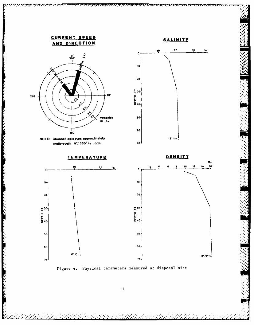
10. The highest current velocity measured during the fieldwork was a

single value of 1.4 fps just beneath the water surface. Sustained maximum

values in the upper third of the water column were more typically 0.4 to

0.8 fps. Sustained maximum values near the bottom were approximately 0.2 fps.

The recording current meters showed frequent periods during which current

velocities were less than the instrument threshold value of approximately

0.05 fps. Figure 4 presents a current rose representative of site conditions

at the actual time of the disposal.

- Background water quality

11. Ambient salinity, temperature, and density data are also presented

on Figure 4. Bulk samples of the water at both the dredge site and the dis-

posal site were obtained two days prior to the start of dredging for analysis

of background chemical constituents and for use in elutriate tests. Results

of these chemical analyses are shown in Table I as background values.

10

o 1k ..

%7Ti

CURRENT SPEED SALINITYAND DIRECTION

o10 2P 3pO %o

20

0* 4Z0 %

a.r0.0

60-

180

NOTE: Channel axis runs approximately 60 210%o.

north-south. 00/3600 is north. 70

TEMPERATURE DENSIT

10 2260 10 1? 14 16

10- 10

20 20

W. 30

0s40- 040

50- s0

601 60

(11,C) 15 5)70 70

Figure 4. Physical parameters measured at disposal site

Table 1

Chemical Analysis of Background Water Samples

TotalSuspended*

Sample Location Solids, mg/k Copper, mg/k Lead, mg/k Zinc, mg/.

Disposal site 5.2 0.015 0.012 0.090 '

Dredging site 10.7 0.014 0.005 0.480

Polychlorinated Biphenyls, mg/"'1016 1221 1232 1242 1248 1254 1260

(Detection Limits: 0.0005 0.0010 0.0005 0.0005 0.0001 0.0001 0.0001)

Disposal site ND ND ND ND ND ND ND

Dredging site ND ND ND ND ND ND ND

* Averages of several samples.

Description of Sediments

Physical

12. Initial sediment sampling was performed by NPS. The contaminated

sediment to be dredged from the shoal area consisted of a sandy, clayey silt

identified as MH under the Unified Soil Classification System. The physical

and engineering properties in the surface layer of the bottom material at the

disposal site were very similar to those of the shoal material. The uncon-

taminated material to be used for capping was a uniformly graded sand (SP).

Representative engineering properties of each of these materials prior to

dredging are summarized in Tables 2 and 3 based principally on analyses by the

NPS laboratory.

Chemical

13. Samples of the sediment to be dredged from the shoal area were also

analyzed by the NPS for chemical constituents. The results of this initial r----

analysis are shown in Table 4. Sumeri (1984) states that a subsequent series

of tests on similar samples from the shoal also revealed the presence of poly-

chlorinated biphenyls in low concentrations. Volatile solids ranged from 2 to

10 percent. -

12

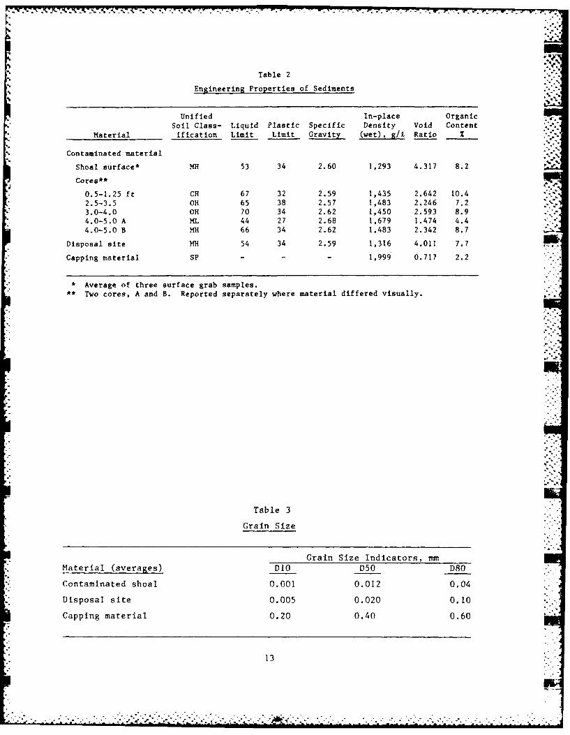
Table 2

Engineering Properties of Sediments

Unified In-place OrganicSoil Class- Liquid Plastic Specific Density Void Content

Material ification Limit Limit Gravity (wet), g/ Ratio I

Contaminated material

Shoal surface* MH 53 34 2.60 1,293 4.317 8.2

Cores**

0.5-1.25 ft CH 67 32 2.59 1,435 2.642 10.42.5-3.5 OH 65 38 2.57 1,483 2.246 7.23.0-4.0 OH 70 34 2.62 1,450 2.593 8.94.0-5.0 A ML 44 27 2.68 1,679 1.474 4.44.0-5.0 B NH 66 34 2.62 1,483 2.342 8.7

Disposal site MH 54 34 2.59 1,316 4.011 7.7

Capping material SP 1,999 0.717 2.2

* Average of three surface grab samples.

** Two cores, A and B. Reported separately where material differed visually.

Table 3

Grain Size

Grain Size Indicators, mm

Material (averages) DIO D50 D80

Contaminated shoal 0.001 0.012 0.04

Disposal site 0.005 0.020 0.10

Capping material 0.20 0.40 0.60

13

_ ..o . .J

Table 4

Bulk Sediment Analyses from the Contaminated Shoal to be Dredged

Concentration ConcentrationElement ppm, dry wt. Element ppb, dry wt.Beryllium 0.2 Acetone 494

Cadmium 1.4 Methylene chloride 805

Chromium 35 bis (2-ethylhexyl) phthalate trace

Copper 130 Di-n-octyl phthalate trace

Lead 190 Aldrin 180

Arsenic 22 Heptachlor 80

Mercury 0.31 4,4'-DDE 30

Nickel 20 4,4'-DDD 80

Selenium 0.4 Alpha endosulfan 30

Silver 1.5 Endrin aldehyde 30

Zinc 240

PCB - 1242 1.4

PCB - 1260 3.1

Dredging and Disposal Operations

14. The planning of the dredging operation represented a balance of

objectives. It was, of course, imperative that the shoal be removed to an

extent sufficient to satisfy navigation requirements. However, for the pur-

pose of the demonstration, it was desirable to limit the disposal to a single

barge load that could be placed in one instantaneous disposal operation.

Through the efforts of the District personnel, both objectives were met.

15. A conventional clamshell dredge was selected to remove the shoal

material. This type of equipment permits sediment to be removed at nearly in

situ densities, minimizes entrainment of site water, and allows a greater

degree of control in loading the transport barge. The intent was to begin the

disposal phase with the contaminated material in a dense, cohesive mass which

could be expected to descend into the depression quickly and with minimum dis-

persion. The transport barge was a split-hull, bottom dumping barge con-

trolled by a separate tug.

14

7,,... ***. *

16. Dredging took place on 26 March 1984. The conventional operation

of the dredge was modified in one respect to help achieve the intent of pro- L"%.

ducing a cohesive mass of material for disposal. Clamshell bucket loads of

sediment were carefully placed in the bottom of the barge rather than being

allowed to free-fall from above the barge as in a more typical casting cycle.

Subsequent estimates based on measurements of barge displacement and material '-u

characteristics indicated that approximately 1,100 cu yd of contaminated mate-

rial was dredged from the shoal area. In a further effort to increase the

cohesive strength, the material was allowed to consolidate in the barge over-

night before disposal. This also allowed the disposal sequence to be timed at

the most favorable point in the tidal cycle. The manner of handling the sedi-

ments described is certainly unique to the requirements of this demonstration

project and would result in some loss of production and increase in cost if

applied in a larger scale project. Note, however, that for any project

involving contaminated sediments, overflowing of the barges for economic pur-

poses is likely to be prohibited and a slower, more deliberate placement of

material in each barge will probably result as a matter of course.

17. The time selected for disposal was near low tide on the morning of

27 March. This higher of the day's two low tides produced a water surface

elevation approximately 6 ft above the datum (MLLW) and resulted in a maximum

depth at the disposal site of 70 ft. Currents were expected to be weak and

variable for at least 2 to 3 hr. The split-hull barge was initially maneu-

vered by the tug into an approximate location over the selected depression.

This was adjusted to a more precise posit'on using directions from District

survey personnel onshore with electronic-optical distance measuring equipment

and theodolites. Barge position adjustments continued to be made as necessary

during the disposal. Sumeri (1984) describes the positioning equipment and

procedures in greater detail.

18. On signal, the barge hull was opened and the mass of contaminated

material exited through the open hopper bottom in approximately 19 sec. The

descent was traced by surface observers and by side scan sonar. Indications

were that the material moved rapidly to the bottom as a well-defined, cohesive

mass.

19. Capping operations were not begun until the next day to allow time

to accomplish sampling and monitoring tasks following the disposal and to

again take advantage of lower tidal current velocities. The capping sand was

15

. * ...

V . - - - ~ - * .' . ra -- -7 ~--

not released as a single mass, but was to be "sprinkled" at a controlled rate

over the entire disposal area. It was expected that this method would reduce

the chance of displacing the soft shoal material and would provide better

overall cap coverage of the site. The sprinkling process was accomplished by

slowly opening the barge hull in small angular increments over a period of 45

to 60 min. A few short periods were observed during which the sand bridged in

the hopper, but in general the sprinkling process performed as expected.

Three barge loads totaling approximately 4,000 cu yd of sand were placed over

a period of 3 days. Hydrographic surveys on 25-ft centers were run across the

site after each capping operation to verify results and to allow for reposi-

tioning of subsequent loads as necessary to ensure complete coverage.

Scope of Sampling and Monitoring

20. Considerable effort and resources were devoted to sampling and mon-

* itoring throughout the dredging, disposal, and capping phases. A brief

description of the scope of these efforts follows. Greater detail on each

task will be presented with the results in subsequent parts of the report.

21. Discrete samples were taken in the water column for subsequent

chemical and physical analyses. These samples were taken during all opera-

tions at the dredging and disposal sites and at a reference site in the water-

way near the disposal area. In each case a number of sampling stations were

occupied before, during, and after each phase. Water samples were obtained by

several types of equipment, but typically were drawn from near-bottom, mid-

depth, and near-surface points at each station. Samples were analyzed for a

variety of chemical constituents as well as for total suspended solids. In

addition to the discrete samples taken for chemical analysis, nephelometry

equipment was employed to continuously monitor turbidity levels. Temperature,

salinity, and current measurements were also made from the sampling boats.

22. Side scan sonar was employed in several situations during the proj-

ect to evaluate its potential as a monitoring tool for such work and to pro-

vide verification of other methods. Sonar images were made of the bottom of

the shoal area before and after the dredging, of the actual descent of the

sediment from the barge to the disposal depression, and of the turbidity

plumes during both operations.

16

... .... . . . . * *.

23. Samples of sediment at each stage of the project were taken by grab ..

sampler and/or vibracore for physical and chemical testing. Multitiered set-.. ,t

tlement plates were fabricated and emplaced to measure volumetric changes in

the dredged material and cap at the completed disposal site. Divers assisted

in all operations and provided visual confirmation of conditions and

locations.

24. Throughout the entire project District personnel supported the mon-

itoring with survey and positioning expertise. Bottom profiles were provided

on 25-ft centers before and aftei disposal of the contaminated sediment and

after each capping sequence. Positions of water sampling station, settlement

plates, and cores were also verified.

--

. .. '

C..77i

PART III: CONFIGURATION OF COMPLETED MOUND AND CAP

Dredged Material Mound

25. The hydrographic surveys supplemented by side scan sonar and subse-

" quent diver observation were used to determine the accuracy of the material

placement in the depression. Successive overlays of bottom profiles (adjusted

"" to datum) before and after the disposal and after each capping increment pro-

vided a clear time sequence of the disposal site construction. Figure 5 shows

two examples of such profiles at different stations within the disposal area.

Note that the vertical scale is greatly exaggerated. Side slopes in the orig-

inal depression ranged from approximately IV to 5H to as steep as IV to 3H.

26. The profiles indicate that the dumping phase of the disposal was

- generally successful in accurately placing the contaminated sediment into the

selected depression. The material descended to the bottom as a relatively -

cohesive mass and struck the targeted portion of the site with little or no

deflection by currents. However, some profiles (e.g. Figure 5) show areas in

which a volume of sediment has been deposited on the waterway bottom outside

the depression. Two explanations seem plausible. Either the force of the

.- impact was such that a portion of the contaminated material surged up the side

-" slope (3-4 ft) and came to rest on the bottom adjacent to the depression; or,

". the impact displaced a volume of soft, surface sediment originally lining the

depression. Analysis of cores subsequently concentrated in this area should

*" establish which process occurred.

27. The profiles were used to produce contour overlays of the original

bathymetry showing the thickness of the contaminated material across the site

immediately following disposal (Figure 6). As shown, the center of mass of

the placed material is clearly within the confines of the disposal depression.

The deposited material was just over 3 ft thick at its thickest point. The

symmetry of the thickness contours and the steepness of the slopes within the

material as indicated in Figure 5 are likely due to the cohesive nature of the

descending mass. Even the portion of the load (or bottom sediment) that

surged out of the depression appeared to have detached itself as a well-

defined mass that came to rest intact rather than flowing in a dispersive,

*radial pattern.

18

" " '" " " '" " " ' " ' ' 'm -' ; ' ' : '' " ' -'""-' " ' '; " "' -' :" " " ..."" " ' • '" ' ' ' " " " " i T h"5:,:

ea -

62-

84 -

i STA 2+25

58 .

so LEGEND 'i

CONTAMINATED DREDGED

MATERIAL (MH) t lI-Jbi62

CAPPING MATERIAL (SP)

STA 1+25

I,, DISTANCE. FTFigure 5. Typical composite profiles through completed disposal mound

28. The dimensions of the hopper in the barge from which the disposal

was made were 128 ft long by 40 ft wide (Sumeri 1984). From Figure 6 it can

be seen that almost 40 percent of the total volume remained on the bottom in

an equivalent size area, never leaving the limits of the barge "footprint"

p during the exit, descent, and bottom collapse. A volume roughly equivalent to

20 to 25 percent of the original volume appears to be contained in the

detached portion of the mound.

Cap Placement

29. Similar procedures were used to sketch thickness contours of the

completed cap as shown in Figure 7. The central area represents a cap thick-

ness of at least 3 ft with the majority of the site having a cover of I to

2 ft of clean sand. The cap was placed in three successive,

19

S...- -

-1. D ...

LIIT OF UNELYN

Figure 6. Co Tso hicknes tus of tecominated mateiaive the disposal mound

20

F u -, 7-

parallel-positioned, overlapping operations. The pattern effects of the three

different disposals can be seen in Figure 7. The desired overlay and unifor-

mity of cap thickness over the entire site are clearly shown. The profiles

produced after the contaminated material was placed show the portion of the -

material that had surged out of the depression and the coverage of this area

achieved by the incremental capping technique.

30. Figures 4-6 also indicate that even though the combined thickness

of contaminated material and capping material approaches 7 ft at some points,

the elevation of the completed site is at or below surrounding bottom eleva-

tions. Continued mound consolidation will further ensure that the disposal

area remains essentially a concave feature with respect to adjacent bottom

topography. While this is not considered a requirement for successful CAD

design, it is felt to be a desirable condition where possible. Such a condi-

tion should reduce the effects of any currents present in the area. A highly

depressed cap surface with abrupt side slopes could be counterproductive by

inducing turbulence at the discontinuity.

7-

21

... - -. ..-- *. - . . .. . " .* ... *..-. ... .- i '. "-: " = " < : " . . ,

PART IV: VOLUME AND MASS BALANCE '-

Volumetric Considerations

General

31. Volumes of both the contaminated sediment and the capping material

in place after the disposal operation were calculated using the profiles pro-

vided by the NPS. The cross-sectional areas of each of the materials on the

profiles were computed using an electronic digitizer/planimeter. A number of

trials were averaged to improve accuracy. The total volume of cap and dredged

material was then calculated using the average end area method. The results

indicate that 975 cu yd of contaminated shoal material could be identified on

the profiles together with approximately 3,700 cu yd of capping sand. This

apparent "loss" in volume, from the 1,100 cu yd estimated in the barge led to

a more in-depth investigation of the processes and accuracy of calculating

such balances.

*' Error considerations

32. The calculation of volumes from average end areas of adjacent cross

sections requires the assumption that variations between profile stations are 5essentially linear. In the case of the Duwamish study, this assumption

appears reasonable because profiles were taken on 25-ft intervals and naviga-

tion references onshore were within a few hundred feet. Any errors in the

results should be directly related to accuracy of the depth measurement itself

or possibly to datum corrections. Variations in navigation position, the

assumption of linear changes between tracks, or long-term bias errors are not

likely to have significant effects in this study. This situation is quite

different than much of the previous work on mass (or volume) balances at sub-

aqueous disposal sites. In most open-water site investigations, intervals

between profile replicate tracks are more typically 25 m (82 ft), making the

assumption of linear variations much more questionable. Also, the survey

tracks frequently extend over lengths approaching 800 m (2,624 ft) and are at

sites several miles from navigation reference station. In such cases, a more

usual approach to volumetric calculations is to produce computer-aided plots

of bathymetric contours from the profiles. The volumes are then computed from

area measuremert within the plot and from the contour interval.

22

gP

,*. . **.. * **

33. Massey, Morton, and Paquette (1984) describe the details of a volu-

metric and mass calculation and offer a method for estimating associated ran-

dom errors. This method recognizes that, in general, random errors can arise

from both depth measurements and position inaccuracies along a profile track.

Further, all volumetric calculations rely on differences between two sets of . ... '

profile data, e.g. predisposal and postdisposal, and each survey has indepen-

dent associated error potential.

34. Appendix A presents a detailed application of this error analysis

to the Duwamish data. The results show that typical random errors in the sur-

vey process could result in errors in the volume calculation of 90 cu yd or

just over 8 percent of the estimated 1,100 cu yd placed. The volume calcu-

lated from the averaged profiles of 975 cu yd is outside this range and is

therefore statistically distinguishable from the original value. It must be

concluded that the contaminated material underwent a volumetric reduction

during the transport/placement processes.

35. It is worth noting that if any one of Lae error source estimates of

±10 cm described in Appendix A had been applied as a uniform bias over the

entire site, the resulting error would have been over 900 cu yd or 90 percent.

This points out the effect of the type of analysis used and the need for great

care in the calibration of instrumentation and in the adjustment of replicate

profiles to an accurate common datum. This analysis also reinforces the

potential pitfalls of accepting volumetric balances directly as mass balances.

A volumetric reduction does not directly imply that the entire amount of mate-

rial was actually lost from the area.

Mass Balance Considerations

Void ratio

36. A number of assumptions must be accepted in order to balance mate-

rial on a volumetric basis rather than a mass basis. Perhaps the fundamental

consideration Is that any changes in the void ratio of the material throughout

the dredging, transporting, placing, and capping operations are taken into

account. Void ratio is defined as the total volume of void or pore space in a

sample divided by the volume of the solids. If the time for the dredging

operation is short enough so that any volatile solids present are assumed to

not be lost, then the volume of the solid fraction can be taken as a constant.

23

Any changes in volume (other than true losses) must then be related to changes

in the volume of the voids in the material. However, these changes in void

space reflected by changes in the void ratio are usually not measured

directly, but are calculated from measured changes in water content of the

material. All calculations of void ratio are directly dependent on the accu-

racy of measuring water content changes and the degree to which the samples

represent the condition of the material.

37. Studies have shown that clamshell dredging tends to produce less

change in the in situ condition of the dredged material than other types of

dredging. However, there is still a slight addition of water to the load as

it is lifted through the water column. Some displacement, i.e. removal of

excess water, then takes place as additional buckets of material are stacked

in the barge. When the barge load of dredged material subsequently descends

through the water column during the placement operation, additional water may

be entrained in the mass. Finally, initial consolidation of the mound by

.- self-weight and by the placement of the capping layer causes a loss of water.

(Of course, consolidation continues for a considerable period of time and fur-

ther affects the water content and apparent volume of material.) In summary,

even during the relatively short time frame of the actual capping operation,

at least four opportunities exist for changes in the water content and void

ratio of the material that could cause errors in using a volumetric approach

to tracking the fate of the dredged material.

38. Table 2 showed that the contaminated shoal material had an in situ

void ratio ranging from 1.5 to 4.3. Specific gravity averaged 2.60. Moisture

contents (weight of water weight of solids) were also measured and ranged

from around 60 to 170 percent. Bulk density (wet) averaged 1,425 g/Z. The

ranges of void ratio and moisture content appear very wide. However, they

reflect the expected increase of sediment density with depth into the bottom.

It is difficult to establish a meaningful, representative single value since

dredging takes place through each depth/layer to different degrees.

39. Samples of the same material were taken directly from the disposal

barge the day after dredging was completed and subsequently analyzed at WES.

The average bulk density (wet) of the material in the barge was 1,464 g/k com-

pared with the average density in the shoal of 1,425 g/Z. Since no solids

were gained, the apparent increase in density must have been due to a decrease

in void ratio and a reduction in the moisture content from consolidation and

24

drainage in the barge. In fact, the moisture content of material in the barge

prior to disposal was measured to be 99 percent. The void ratio was then cal-

culated to be 2.6, confirming the reduction indicated. It should be noted

that some free water was observed on the surface of the material in the barge.

This was evidently water added by the bucket during dredging and the small

actual amount freed during the change in void ratio. It appears that any

water added by the bucket dredging process did not readily find its way into

the pore space of this soil and is an addition only in the sense of bulk vol-

ume. At the time of disposal the material was in a similar or slightly denser

state with greater internal strength than it was in situ. Figures 8 and 9

show the dredge placing material in the barge and the surface of the material

in the barge after loading had been completed.

Initial mass

40. Obviously, a mass balance must begin with the calculation or esti-

mation of some initial mass of material. Tavolaro (1983) provides one of the

few attempts at a mass balance calculation using data collected from several

projects in New York Harbor. In that study he approached the calculation of

the initial mass as follows. Cores of shoal material were obtained prior to

dredging and tested for in situ bulk (wet) density and water content. These

density values were converted to dry specific weight using relationships pro-

posed in previous work. The initial dry mass of material in situ was simply

this dry unit weight multiplied by the volume it occupied. However, to obtain

the volume, he compared bathymetric surveys of the sites before and after

dredging.

41. This method of calculating the initial mass is dependent on the

accuracy of the volume determination and the survey. With the exception of

the water depth, conditions and equipment used at the Duwamish dredging site

were very similar to those at the Duwamish disposal site. It is therefore

reasonable to assume that the error analysis earlier in this report for volu-

metric considerations at the disposal site would apply to calculation of the

excavation volume at the dredging site. This analysis indicated an error

range on the order of 8 percent. If the above approach were applied to the

Duwamish data, the resulting initial calculated mass would be accurate to not

better than ±8 percent.

42. If, on the other hand, the balance begins with the mass as measured

in the barge after dredging, the mass of the solids which were suspended

25::

Figure 8. Clamshell loading barge during dredging operation

Figure 9. Contaminated material in barge prior to disposal

26

during dredging and transported out of the area will not be counted in the

balance. (Those solids which are suspended but drop back to the bottom at the

site are not considered "lost.") However, in the New York Harbor work the

mass of solids which was indeed lost between the in situ condition and the -' [

loaded barge was reported as 2 to 3 percent of the total mass of material

(Tavolaro 1983). This level of loss could not be identified with confidence

using the standard bathymetric surveying techniques. Keeping in mind that the

primary objective of the WES involvement in the Duwamish project was to eval-

uate capping and that the placement/capping phase follows from the condition

of the material in the barge, the mass balance was started at that point as

well.

43. Bokuniewicz et al. (1978) presented a method for determining the

bulk density of materials in a hopper. The formulation uses differences in

the vessel's draft for various loadings and the total hopper volume and has

been applied with success by Tavolaro and others. The resulting bulk density

is then converted to dry density and multiplied by the hopper volume to pro-

duce a value for dry mass present. However, care must be used in its appli-

cation in that the assumption is made that the container, i.e. the hopper, is

loaded to the same internal level in preparing the capacity plan for the barge .'-

as when loaded with dredged material. This is accomplished in a practical

sense by placing material until the hopper is "full" (and usually deliberately

overflowing). In the Duwamish project the barge was not filled to its level

capacity and overflowing was not allowed. The bulk density cannot be calcu-

lated directly from the equation as given by Bokuuiewicz.

44. The mass of material in the barge can still be estimated by bypass-

ing the question of bulk density and calculating the weight of material pres-

ent directly from the drafts of the barge. Careful measurements of the barge

drafts at each of the four corners were made with the barge empty and with the

partial load of contaminated material. From a Properties of Form table pro-

vided by the contractor for the specific barge used, the weight of the mate-

rial in the hopper can be calculated from the displacement. This is, in

effect, the basis for the equation proposed by Bokuniewicz, but without the

hopper volume term simply yields the weight directly rather than density. The

wet weight of the material in the hopper was found to be approximately

1,366 tons. The dry weight can be calculated as follows using an average

moisture content in the material:

27

. . . . .-. .

* * w ,.,. .. ,.

o'

Ww

w mis(r1)ntn

D (I-+-W)

where

bgnW odry weight of materialD

W h= wet weight of materialw = moisture content

* The results using the measured moisture content of 99 percent indicate that

approximately 686 tons of solids (dry weight) were present in the barge at the

beginning of the disposal operation.

l~osses at disposal site

45. The time between dredging and placement of this material was so

short that potential losses due to oxidation of organics present were not

included in the balance. Therefore, the primary sources of material loss were

resuspension during descent and flow on impact. As described earlier, the WES

monitoring effort included extensive sampling to determine the load of sus-

pended solids in the water column. Samples were taken along three radials

extending from the barge at the point of disposal. Stations were occupied at

varying distances from the barge along the ralials. The closest station was

located approximately 50 ft from the center of the barge and the farthest sta-

tion was just over 800 ft from the site. At each station discrete samples of

water were taken at several depths in the water column as rapidly as the sam-

pler could be cycled through the depths. This provided a reasonably contin-

uous time series during the first 30 to 40 min after disposal. The sample

time intervals were increased thereafter to 5 min, then to 10 min, and finally

to 20 min for approximately 3 hr after disposal. Samples were returned to an

analytical laboratory and tested for total suspended solids (in addition to

other parameters).

46. One method which attempts to quantify the mass of sediment lost due

to resuspension takes a single average value for the suspended solids concen-

tration throughout an area and multiplies it by the volume of the water in the

area or basin. This approach essentially ignores (or considers only in the

averaging process) any variations in the concentration with time or depth.

Results are at best a very rough estimate. Hayes, McLellan, and Truitt (1985)

have suggested a method of analyzing suspended solids data that may provide a

28 A

.7- -

S . . -.

- - r rV% 7 7_77,,7. 77. - 7 7.---7

first level of refinement to such calculations. In this approach the values

of suspended solids concentration measured from discrete samples taken at

varying depths are assigned or averaged over only an increment of depth at

which they were taken. This replaces a single depth-averaged value with a

series of concentrations associated with a number of "slices" through the

water column. Further, as shown in Figure 10, the depth scale itself is nor-

malized by the total water depth at the station in order to present the values

as an incremental percentage of depth. This allows comparison of relative

concentrations at stations with different water depths.

II 68 ,

8 I ii iiIIIi~ l!I'II

7~!!i M ill

I I, I I II ',-

D 40 i% i'i I i, '-

P i

188 8 2 4 6 8 18 12 14 16 18 28

TOTAL SUSPENDED SOLIDS, xl0 g/L

Figure 10. Typical representation of total suspended solids

from single sampling event

47. In contrast to the dredging operation itself, the actual disposal

was a short-term event. The variation of solids concentration with time

during that period is an important factor. Figure 11 is a plot of total sus-

pended solids versus time after disposal at a representative station approxi-

mately 400 ft downcurrent from the disposal site. The three different curves

represent samples taken near surface, mid water column, and near bottom.

Background levels of solids at the time were measured as typically 5 mg/Z or

less and the values shown in the figure have not been adjusted. The rela-

tively rapid passage of a very distinct solids plume can clearly be seen.

48. For this study the following approach was used. A cylindrical

control volume in the water column is assumed at the point of disposal, the

29

* .. ;

ELAPSED TIME AFTER DISPOSAL STARTED - minute,

0 42 Is 2 0 24

Too

600

MEAfN BOTTOM SAMPLEIS

E 600

. .4

0

aooo ,

toot

o .

0

Figure 11. Time series of total suspended solids at typical

station following disposal

radius of which is nominally the dimension of the disposal depression itself.

This volume is taken as the source of solids leaving the site by both resus-

pension during descent and flow after collapse. The flux of suspended solids

passing through an appropriate portion of the surface area of this cylinder is

then the loss of mass from the site. It is recognized that particles will

settle out of suspension continuously as they progress radially from the dis-

posal point. However, the distribution of concentration with time or radial

distance is not necessary for mass balance. The mass that reaches the bottom

within the limits of the cylinder is not lost from the site. That mass which

passes through the surface area is lost from the site regardless of where it

ultimately comes to rest. This approach also requires a near-field viewpoint

of the transport process. The assumption is that advective transport domi-

nates over diffusive processes at least to the limits of the control volume.

Data from a station approximately 50 ft upcurrent from the disposal point

30

i '* * -.d.-

* *.. b ~ A ) 2 .1 ..-.

indicate that the concentration of solids in the mid and upper water column

did not increase above typical background levels. A peaked distribution sim-

ilar to that shown in Figure 11 was observed at the near-bottom sample series. -

This supports the assumption that advective processes, e.g. currents and

momentum driven flow, were the principal sources of transport within the lim-

its of the disposal site itself.

49. Using this approach, the mass of material lost from the site during

the disposal can be estimated as follows. A weighted, time-averaged value for

the solids concentration during the passage of the plume is computed for each

of the three sample depths at the representative stations. An effective

transport rate at the station can be estimated from calculating the velocity

of the solids plume using the time of arrival at the station. Again, this

velocity is computed separately for each of three depth increments and the

resulting transport rate is the velocity multiplied by the depth increment and

by a unit width or arc length along the control cylinder. The incremental

loss of mass is then simply the transport rates multiplied by the correspond-

ing time-averaged concentrations. This value still represents only the mass

lost per unit arc length and an appropriate length must be selected to calcu-

late the total mass leaving the site. The length selected is certainly some-

what subjective, but should at least consider factors such as the distance to

the solid bulkheads paralleling the site and the width of the flow projected

in the direction of the currents.

50. The result of the application of the above method indicated that

losses during the disposal operation were on the order of 50 to 100 tons of

solids. This is on the order of 7 to 15 percent of the total mass calculated

in the barge prior to placement. Note that using a nominal wet unit weight of

90 pcf, 50 tons of solids is actually only 41 cu yd of material or less than

4 percent of the original volume. The losses could not be distinguished

within the 8-percent error limits of the volume calculation.

Final mass

51. Paralleling the above discussion of the initial mass, the calcula-

tion of the final mass in the mound is also dependent on a volume computation.

The volume identified in the mound was 975 cu yd within an accuracy of 8 per-

cent. Vibracore samples were taken in the mound immediately after capping and

the sediment was tested for the same parameters as the shoal and barge

samples. The moisture content in the mound material was found to average

31

.- °

* r;r! dj.r :rVc r. . - .r -

86 percent and the bulk (wet) density averaged 1,509 g/t. After adjusting for

the moisture content and multiplying by the 975-cu-yd volume, the calculated

dry mass in place in the mound was estimated to be 666 tons.

Balance

52. A simplified mass balance can be stated using the above results.

The balance is simplified in the sense that the initial mass was taken as the

in-barge condition so that losses at the dredge are not included, nor are any

potential losses due to volatilization of solids. The balance is then,

/Dry Weight of.}.

Dry Mass - Solids Lost = Dry Mass in (2)(in Barge) (During Disposal (Disposal Mound

* and, substituting values from above including error limits,

686 tons - to 100 tons) (666 ± 53 tons)

or,

(636 to 586 tons 719 to 613 tons)

Clearly the ranges overlap and the mass does balance within the accuracy of Wthe measuring processes.

53. Sources for the differences in the terms could include nonrepre-

sentative material samples (especially effects of the vibracore), variations

in geotechnical testing procedures, or underestimation of any of the several

error sources identified in the survey/volume computation. In general, most

-- of these considerations would serve only to widen the error limits. The two

readily identifiable factors that would actually change the calculated masses

are densification of the samples by the vibracore, and any uniform bias in the

survey, e.g. datum adjustments, tides, etc, that would incorrectly estimate

the volume in place. Problems with both factors are possible and even likely.

However, the equipment, techniques, and expertise used in both procedures rep-

resent the accepted practice in the field and the resulting balance with an

uncertainty in the range of 8 to 10 percent may be the best available at this

* time and for this level of monitoring effort.

32

Mound Consolidation

54. In order to evaluate the long-term stability of the constructed

disposal mound it is necessary to distinguish changes in elevation (and vol-

ume) resulting from erosion and transport of material from the site and from

consolidation of the mound itself. Consolidation can occur in the cap mate-

rial, the contaminated dredged material, and in the underlying bottom

sediments. This portion of the WES study was directed toward careful evalua-

tion of consolidation from each of these sources and the development of infor-

mation that will lead to a better understanding of the consolidation process

in subaqueous dredged material deposits. -55. Settlement plates were placed at the site prior to disposal opera-

tions to facilitate monitoring of consolidation in the materials over time.

These plates were of tiered design so that changes in each of the materials

could be evaluated independently. A telescoping arrangement permitted place-

ment of the lower plates on the foundation soil prior to disposal, the second

tier on the surface of the dredged material, and the third tier of plates on

the surface of the cap (Figures 12 and 13). Plates were installed by divers

and initial readings of e:, ised riser lengths were noted. The lowest level of

plates was anchored to the bottom using helical earth anchors. In spite of

this anchoring arrangement, the impact of the dredged material on the bottom

after disposal was so violent that several of the plates were overturned and

lost. The presence of I to 2.5 ft of very soft organic silts (ML, MH)

overlying more sandy foundation materials is believed to be a major factor in

the instability of the settlement plates. Readings of the remaining usable

tiers were made after each phase of the disposal, after approximately 1 week,

and after 6 months. Analysis of the data is continuing, but readings indicate

that the original 24- to 36-in. thickness of deposited dredged material has

consolidated to 21 to 33 in. in the 6-month interval. The consolidation pro-

gressed rapidly with approximately 75 percent of the total settlement to date

occurring in the first week after placement. Little change has been noted in

the thickness of the sand cap.

33

_____.PIPE RISER

p 4-" ~ PIPE RISER

_____________________2' PIPE RISER

,,-:OVERLYING WATER

MARINE GRADE

PLYWOOD WITHSAND CAP STEEL BEARING PLATE-

ORIGINAL BOTTOM

Figure 12. Schematic of tiered settlement plates

Figre 3.View of settlement plates prior to placement

Figure 13

PART V: SIDE SCAN SONAR MONITORING

General

56. The WES Coastal Engineering Research Center provided side scan

sonar (SSS) monitoring of the dredged material disposal in the Duwamish Water-

way in Seattle in March and April 1984. The following sections from Clausner

(1984) describe the SSS phase of the Duwamish field project.

57. The primary mission in the monitoring operation was to use SSS to

measure the time for the initial mass of disposal material to reach the bot-

tom, a value needed for verification of a mathematical model. This was accom-

plished successfully. A secondary objective was to determine the extent of

the sand cap. This second objective was only partially successful primarily

due to environmental constraints. Also, SSS inspection of the actual dredging

operation was accomplished and proved to be successful in locating the sedi-

ment plume in the water column. Appendix B (Clausner 1984) provides a summary - -

of the background and principles of SSS operation for those readers not famil- --

iar with the equipment.

Operations

Initial observations

58. On 24 March 1984, the SSS and other water sampling equipment were

loaded aboard the WALTON, a 31-ft work boat. The SSS "fish" was deployed from

a wheel and pipe clamped to the stern of the boat. This method of deploying

the "fish" worked well throughout the operation.

59. The depression into which the dredged material would be dropped was

approximately 150 ft wide, 300 ft long, and 6 to 6.5 ft deep, with the long

axis of the hole positioned perpendicularly to the axis of the Duwamish Water-

way. Bottom surface sediments are uniformly solt silts, and the water depth

at the site was 55 to 65 ft deep.

60. The narrow waterway (approximately 750 ft wide) with its vertical

sides, heavy traffic, and industrial operations made producing good SSS images

of the area very difficult. In addition, a large container ship was contin-

uously tied up to the western bank, reducing the effective width of the

35

.. .. ....... "..".........."............. "."...."...... "....".... ".............'..'.'....".....".....'."...-. . - h*

waterway another 100 ft. Also, the area is heavily trafficked, with tugs

pushing barges through regularly.

61. The 100-kHz "fish" was used first. The hole was easily located,

showing up as a depression in the bottom trace. However, the soft material, .. *"

gentle slopes, and high level of background noise made topographical features

* of the hole impossible to distinguish on the record. Reference rods (2-in.

outside diameter steel pipes), plates, and subsurface buoys, placed by divers

in the depression prior to the SSS survey, were slightly visible on the

100-kHz record. Runs parallel to the long axis of the hole were very diffi-

cult. By the time the "fish" stabilized after making the turn, the boat was* already over the hole. As the "fish" was reaching the end of the hole, the

,- boat had to turn to avoid the dock or the moored ship. Also, the changes in

speed caused by the turn caused the "fish" to move up and down, making eval-

uat-ing the bottom elevation changes impossible.

62. A significant problem was experienced because of self-made and out-

side noise. This was particularly evident when operating the SSS and the sub-

bottom profiler simultaneously. It became very difficult to tune the side

* scan, and the quality of the subbottom record was reduced. The probable cause

is the narrow channel with its vertical sides. Instead of disappearing into

the distance, as is the usual case, the sound energy remains trapped, causing

interference and tuning problems. In addition, there were times when just

tuning the SSS was very difficult. Noise produced by the shipyards and fac-

tories may have been the reason. The interference pattern on the side scan

record made determining textural differences on the bottom impossible.

63. Residual air left in the water from the wake of the WALTON or other

boats distorted the records. After several passes, it became necessary to

stop and wait 10 to 15 min while the water acoustically cleared.

Reference sand disposal

64. One dav before the actual disposal of the contaminated sediments, a

practice or reference sand disposal was made. One purpose of the practice

*disposal was to allow all those participating in the monitoring operation an

. opportunity to become familiar with the procedures and equipment to be used in

the actual disposal. This practice disposal was most important for the SSS

portion of the monitoring effort since it had never been used in this kind of

operation before.

65. For the practice disposal, the SSS was suspended horizontally on

36

premeasured ropes 36 ft below the surface. The 500-kHz "fish" was used. It

was set on the 50-m range, and paper speed was 50 lines/cm. The WALTON was

tied to a tug positioned parallel to the barge at its midpoint (Figure 14).

The addition of the 20-ft beam of the tug caused the SSS "fish" to be 45 ft

from the centerline of the barge.

SPLIT-HULL BARGE

v- WALTON --"

TOP VIEW

SPLIT-HULL BARGE

WAL-TON- TU

SIDE VIEW

Figure 14. SSS positioning during dredged material disposal

66. When the drop started, the sand plume in the water column was such

a strong reflector that the sound signal saturated the record, making the

determination of the time for the material to reach the bottom impossible.

After that time, the SSS record showed that the sand did not drop at a steady

rate but instead came out in a series of concentrated masses. Six individual

masses could be seen, starting at 2, 6.5, 15, 21, 26, and 36 min, respec-

tively. There is a good possibility that the Individual masses seen on the

record may be due to the drifting of the barge which was eliminated on

37

subsequent disposals. Motion by the barge would cause the SSS "fish" to move.

Movement of the sonar beam in and out of the sand plume would cause the

appearance of a sand mass each time the beam swung back into the plume.

67. Post sand disposal inspection with the 100-kHz "fish" and subbottom

profiler set on a 50-m range, towed at a depth of 40 ft, did not reveal any

noticeable changes in the bottom topography.

Dredging operation inspection

68. After the reference disposal, the 500-kHz SSS "fish" was used to

monitor the dredging operation. This operation was very successful. The

Seattle District contract dredge, its spud, the barge, and the dredged area

are all clearly visible on the SSS record (Figure 15). Also, most impor- l

tantly, the dredge plume was visible on the record. The plume can be seen

clearly in the water column for a distance equal to approximately half the

length of the dredge. Analysis of the water samples taken for total suspended

solids confirmed the location of the solids plume at this point. However,

further examination of the records shows a dark area to the right (east and

north) of the dredge and extending at least 200 ft past the back of the

dredge. This dark area was originally postulated to be the water column plume

moving downstream, a concentrated sediment layer near the bottom, a tuning

anomaly, or a change in bottom material or slope. Subsequent review of the

suspended solids data does not support the presence of the plume at that loca-

tion. The channel slope does occur, however, in the same general area.

Contaminated material disposal

69. On the morning of 27 March 1984, SSS was used to time the fall of

the contaminated dredged sediments. The same configuration of the split-hull

barge, tug, and WALTON was used as for the reference disposal. Here, the

"fish" was at a depth of 54 ft (10 ft off the bottom). Based on the reference

disposal experience, SSS gain controls were tuned down so only strong reflec-

tors would produce an image. This was done by towing the "fish" next to the

docks prior to the drop and adjusting the gain controls to produce an image

from the piles but not from the bottom.

70. Fortunately, these settings proved to be correct, and the disposal

was clearly visible on the record (Figure 16). According to the barge opera-

tors, the material did not completely exit the barge until 20 sec after the

start of the disposal. This corresponds exactly with the SSS record (Fig-

ure 16). The material exited the barge at just over 20 sec and hit the bottom

38

P- 17 -7 F.1'

lip,

50'.

A--

Figure 15. SSS image of contaminated sediment dredging.A =dredge, B =dredge's spud, C =barge, D =dredged area,

E =dredge plume, F =dark area, and G log boom

39

-50-,

* SIGN4L DISAPPEARS

BOTTOM IMPACT

205 SEC

~BOTTOM 20iiJ

START, TIME ZERO

Figure 16. SSS image of contaminated sediment disposal

40

• %o

15 sec later. Twenty-one seconds after the material left the barge, the image

disappeared for 24 sec. It is possible that this disappearance was due to the

mud wave covering the "fish." After the image returned at 65 sec from the

start, there appeared to be a substantial amount of material in the water

column on both sides of the "fish." At 2 min 2 sec after the start, the

amount of sediment in the water column was greatly reduced but did not dis-

appear. This could be the result of a change in orientation of the SSS "fish"

due to barge maneuvering. However, the image was not smeared as it usually is

during maneuvering. This water column sediment reduction lasted for 50 addi-

tional seconds. After that point, the sediment content of the water column

increased to about its former level and remained there until approximately

10 min after the start. Past 10 min, maneuvering of the barge made good

observations of the sediment level determination impossible up to the time the

recorder was turned off at 15 min from the start of the disposal.

Inspection of the first sand cap disposal

71. The estimates of the extent of the sand cap in this section and in

the following section are somewhat subjective. Textural differences between

the native bottom clay sediments, the contaminated clay sediments, and the

sand cap were not particularly evident on the SSS record. The tuning problems

discussed previously also made precise interpretation difficult. Finally,

positioning was inaccurate. Not all the range marks were visible, and dis-

tances off the channel and hole center lines had to be visually estimated.

72. Using the 500-kHz "fish," an SSS inspection of the first sand cover

was made on 29 March 1984. After several passes, both parallel and perpendic-

ular to the channel, a fair estimate of the shape and extent of the sand cover

could be made. The shape was basically rectangular (Figure 17) with slight

indentations on the perpendicular axis. It appeared that the cover extended

65 ft north and 90 ft south of the cross channel center line and 70 ft on

either side of the channel center line. However, the dark event line on the

figure representing the center line of the hole is displaced by an estimated

10 to 20 ft to the north. It appears to be on the top of the edge of the

depression instead of in the center. After the event line is moved back to

the center of the hole, the revised estimate for the sand cover dimensions is

75 ft north and 75 ft south of the center line. These dimensions correspond

well to the contours produced from the hydrographic surveys shown in Figure 6.

41...

LI IT

.

J ....' LI...'"..

• NT RE h , l |APPROX I '%(P'

, .. :i..,

,, , .E.~ A S T- WE ST ,_ "'''

V.,

APP-OK 14O-

Figure 17. SSS image of the first sand cap

Inspection of the completed sand cap

73. On 2 April 1984, the 500-kHz "fish" was used to inspect the com-

pleted sand cap. A total of ten passes was made over the drop site. An

attempt was also made to determine the thickness of the sand cap using the

subbottcm profiler. The sound pollution created by using the SSS and subbot-

tom profiler simultaneously seriously degraded the topographic features and

sediment texture differences on the record while producing a poor estimate of

the cap thickness.

42

,T7 7- . .- , I.."

N

IW E ,

CHANNEL

A EDGE OF DARK AREARIDGE AND VALLEY A

9.0 .

- TARGETS

.TARGET

0 . -0

- - 1 - ss ,,+ 50-

DAKAREA

Figure 18. Completed sand cap coverage..

74. Although the quality of the records was too low for good reproduc- .''

*tion, it was possible to make an estimate of the extent of the sand cap. In :

*Figure 18, the outline of the depression is shown along with the tracks of the

*six best SSS passes. On the figure are four features which show the estimated".-".

*boundaries of the sand cap. A north-south running ridge and a valley are seen.-.

*at the western edge of the channel. Dark areas, presumed to be areas covered i

*by sand, are seen to the north, south, and east. Several targets are also i'!

*illustrated. They aided in determining location of the features. The north-

*emn boundary is 35 to 65 ft north of the long axis of the depression, and the "

southern boundary is approximately 100 ft south of the axis. The eastern and

western boundaries are 140 and 150 ft, respectively, from the center line of -.

the channel. It appears that the original depression was completely covered

by the sand cap.

75. As mentioned earlier, the subbottom profiler was used to make an

* estimate of the cap thickness. The quality of these data is not good, but a

rough estimate of the thickness using these data would be about 6 ft, compared,.

wihathickness of3 to 4ft etm edin PatII frmcomparison ofthe rep- -

licate survey profiles.

.9'.,,, .'.. -9-.. . +-...,*.*.*..*.. . ... ..... .. ..... . ,.. .. ... . . ... . .. + ° . . .- -. .. :.-

*q .. .. . , .. * * *. ** . * **~~~* *~ .* .* .- . ~ .. . **.. 00.

Summary

76. SSS was used successfully to monitor a dredged material disposal

operation in Seattle. Timing of the fall of the dredged material was com-

pletely successful once the proper methodology was determined. Monitoring of

the dredging operation provided an unexpected bonus when it was discovered

that the sediment plume in the water could be detected. The more conventional-7

use of SSS to determine the limits of the sand cap cover was successful,

although record quality was limited by channel dimensions and configuration

and noise pollution. Finally, the subbottom profiler was marginally success-

ful at determining the sand cap thickness.

77. The ability of SSS to determine cap coverage or disposal sediment

coverage is a function of grain-size difference between the two sediments.

The greater the difference, the more easily the boundary between the native

and the disposed sediments can be seen. The limiting factor in determining

boundary location is positioning. Even in a small area with many landmarks

and ranges like the Duwamish Waterway, visual estimation of location is dif-

ficult. To accurately locate features on an SSS record, a positioning system,

e.g., a miniranger, is necessary. 578. Determination of disposed material thickness or cap thickness is

possible with a subbottom profiler. For accurate results, a fairly sophisti-

cated unit is needed. However, in most instances, a standard hydrographic

survey depth sounder is still the best tool for determining sediment thickness

from replicate surveys. Only in areas without proper elevation reference

marks and tide data would a subbottom profiler be better for determining sedi-

ment thickness.

44

*[. . . .* . . . . *.

r--. , L

',

PART VI: CHEMICAL STUDIES

79. The portion of the work addressing the effectiveness of the cap in

isolating the chemical constituents in the shoal material from the water col-

umn will not be completed until longer term sampling has been accomplished and

the results analyzed. The following brief summary of preliminary results has

been provided by Dr. James M. Brannon of WES who is performing this work.

80. Sediment samples were analyzed for total concentrations of poly- .

chlorinated biphenyls (PCBs), copper (Cu), lead (Pb), and zinc (Zn) in core

samples from the Duwamish capping sites. This testing was conducted to deter-

mine if these contaminants, which were present in the dredged material but

absent or present in trace quantities in the caps, were migrating upward in

the cap material. Samples were taken within 2 weeks following capping opera-

tions and then 6 months after capping. An additional set of samples will be

taken 18 months after cap placement.

81. Samples were taken for chemical analysis from vibracores taken at

the Duwamish capping site and at an adjacent reference site (cap material

only). After the core had been opened with an electrical circular saw and any

plastic shavings on the sediment carefully removed, the sediment/cap interface

was identified. The interface was usually strikingly evident because of the

textural differences between the cap (sand) and the dredged material (mainly

silt). Ten samples were taken in the cap and seven samples were taken in the

dredged material at consecutive 4-cm intervals on either side of the dredged

material/cap interface. An additional sediment sample was also taken in each

core at various depths below the cap/dredged material interface to chemically

characterize unusual sediment layers.

82. Results of chemical analysis of initial core samples indicated that

the dredged and cap materials formed a sharp, relatively unmixed interface.

This is illustrated in Figure 19, which presents Pb and Arochlor 1242 PCB con-

centratlons in a core at the Duwamish capping site. Both Pb and PCBs were

initially either absent or present in low concentrations in the cap materials. '

Below the cap/dredged material interface, however, high concentrations of Pb

and PCB relative to those in the cap material were noted.

83. Water samples (four) were also taken I m above the sediment at the

capping demonstration site. For comparison purposes, water samples were also

taken either upstream or downstream of the demonstration site at each

45

* , 4 .*..ll l... . ..

48-52 48 5

44- 44

40-44 *40 41436-40 60.

I 336 -

E 30-36 E 326

U 28-31. U 2-32.

j 24 28j 242-

0t -4 1 -C 20-2+-

16320 cc 16-20LU

12-1 6 * 12-16"

-.12 a

Z 46 , 4.

SI- 4 CAP MATERIAL I- CAP MATERIAL* . -- _ __ __ _ a. _ _ _ _ _IL' 04 DREDGED MATERIAL W 044 DREDGED MATERIAL4-8

8' de

812 128-I2 .

12-16, 1216

4b 20 16 20

4-24' 20-24

24-28 " 24 28

0 0 20 30 0 2 4 6

pUg/ g pg/g

LEAD AROCHLOR 1242

Figure 19. Chemical profile through the cap

sampling; selection of the upstream or downstream sampling location depended

on the direction of tidal flux at the time of sampling. These water samples

allowed evaluation of any measurable impacts on water quality due to contami-

nants from the dredged material moving through the cap. Analysis of these

data continues and the final results of the chemical studies will be reported

" in a subsequent document.

46

.- **.** **. *.l* --. *~,-*.- - . *. . .. ,4

PART VII: SUMMARY

84. The Seattle District and the Waterways Experiment Station have

cooperated in a project in the Duwamish Waterway that successfully demon-

strated the engineering aspects of subaqueous disposal and capping of con-

taminated dredged material. Approximately 1,100 cu yd of silty, clayey shoal

material was removed by clamshell dredge, transported by barge, and bottom

dumped through 70 ft of water into an existing depression. The site was then

capped with successive loads of a clean sandy cover. All operational features .,

of the demonstration were completed successfully. This report has analyzed

the results of the initial field operations and the first (6-month) monitoring

effort.

85. The results of bathymetric surveys were reported showing that the

material formed an identifiable mass at the disposal site. The physical

impact of the descending material on the bottom was violent, but subsequent

surges were confined to the immediate vicinity. Approximately 40 percent of

the original volume could be identified in a bottom area equivalent in size to

the "footprint" of the discharging barge's hopper. Maximum thickness of the

mound of shoal material was measured to be 3 ft. The cap covered the disposal

site completely with a thickness ranging up to 3 ft. The ratio of the volume

of capping material required to the volume of contaminated material was

approximately 4 to 1.

86. Discussions of both volumetric and mass balances have been pre-

sented. A volume of material in the depression equal to that measured ini-

tially in the barge could be clearly identified on the surveys. An error

analysis is described suggesting that the accuracy of the volumetric computa-

tion is within approximately 8 percent. Suspended solids concentrations were saw

measured in the water column at both the dredging and disposal sites. Losses

during disposal were estimated to be on the order of 7 to 15 percent of the

initial dry mass. A subsequent mass balance was presented. Differences in

computed values were in the range of only 8 to 10 percent. Possible sources

of error in the balance were examined.

87. Side scan sonar was used in several ways during the dredging and

disposal and an analysis of its utility for such work was presented. A small

solids plume associated with the dredging could be see through the sonar

equipment and the descent of the material through the water column at the

47

disposal site was also monitored. The primary problem noted was the high

level of acoustic background "pollution" in the busy waterway which may make

the application of side scan sonar at such sites more difficult and

time-consuming.

88. Brief scopes have been included summarizing the fieldwork and

intent of associated monitoring of mound consolidation and chemical effective-

ness of the capping procedure. These studies are continuing and additional

sampling and testing will be completed at approximately 18 months following

the original disposal.

Nam-

48

'. m .

~ as, -

... . . . . ..'.. .- V.--

REFERENCES

Bokuniewicz, Henry J., et al. 1978. "Field Study of the Mechanics of thePlacement of Dredged Material at Open-Water Disposal Sites," TechnicalReport D-78-7, US Army Engineer Waterways Experiment Station, Vicksburg, Miss.

Broughton, Jerald D. 1977. "Investigation of Subaqueous Borrow Pits asPotential Sites for Dredged Material Disposal," Technical Report D-77-5,US Army Engineer Waterways Experiment Station, Vicksburg, Miss.

Clausner, James E. 1984. "Side-Scan Sonar Monitoring of Dredged MaterialDisposal in the Duwamish Waterway," Letter Report, US Army Engineer WaterwaysExperiment Station, Vicksburg, Miss.

Hayes, Donald F., McLellan, T. Neil, and Truitt, Clifford L. 1985. "A Tech-nique for the Analysis of Suspended Solids Data," Internal Working Document,US Army Engineer Waterways Experiment Station, Vicksburg, Miss.

Johanson, Edward E., Bowen, Stuart P., and Henry, George. 1976. "State-of-the-Art Survey and Evaluation of Open-Water Dredged Material Placement Method-ology," Contract Report D-76-3, prepared by JBF Scientific Corporation for theUS Army Engineer Waterways Experiment Station, Vicksburg, Miss.

Massey, Alan T., Morton, Robert W., and Paquette, Gary D. 1984. "Mass Bal-ance Calculation," Part IV of Volume IV, Summary of Program Results, DisposalArea Monitoring System (DAMOS), prepared by Science Applications InternationalCorporation for US Army Engineer Division, New England, Waltham, Mass.

Sumeri, Alex. 1984 (Nov). "Capped In-Water Disposal of Contaminated DredgedMaterial," Proceedings of the Conference Dredging '84, American Society ofCivil Engineers, Vol 2, pp 644-653.

Tavolaro, John F. 1983. "Sediment Budget Study for Clamshell Dredging andDisposal Activities," US Army Engineer District, New York, New York, N.Y.

49

................................................

'% -. 7-

APPENDIX A: ERROR ANALYSIS OF BATHYMETRY

1. The error analysis by Massey, Morton, and Paquette (1984)* is based

on weighted averages of depth readings and track errors across a grid square

or cell of arbitrary size. The standard deviation of the calculated value of

the volume is given by:

a =A r2a (Al)V

a s

c rr

where a c . c

and

a= standard deviation in volume calculatedv

A = area of total survey

ac standard deviation of the depth error in any given cellC

M = number of grid cells in the entire survey

a = standard deviation of all measurements of depth in a cellrN = number of individual depth measurements in a given cell

2. The error analysis can be extended to the Duwamish data by making

the following assumptions. An arbitrary grid system can be constructed over .

• the disposal site with the grid size equal to the width of one track interval

or 25 ft. This grid size would result in a 13 by 10 array totaling 130 cells.

The shallower water depths, closer proximity of navigation references, and

more sheltered hydrodynamic environment all suggest that the lower values in

the ranges given for each source of error are reasonable for the Duwamish

data. Fathometer error would then be estimated as ±10 cm. The cross-track

position error would produce errors in the depth measurement of no more than

±10 cm, and short-term fluctuations in the water surface elevation during the

actual survey (waves, tide, boat draft, etc.) could produce errors of ±10 cm

also. The root-mean-square for these three source errors would also be ±10 cm

. and is then the value of a in Equation Al. Using approximately 1.8 as ar

. typical value for N for a 25-ft square cell gives:

* * See Refeteres at the end of the main text.

Al

=r = 10= = 7.45 cm

*then-VM V 3 0

and a AJ~ V" A 2i (0.65) approximately 90 cu yd

A2

APPENDIX B: BACKGROUND AND PRINCIPLES OF SIDE SCAN SONAR OPERATION

How a Side Scan Sonar Works

1. Side scan sonar (SSS) is an outgrowth of the echo sounding depth

finders developed during World War II. It has been used to map the sea bottom

and to search for submerged objcts since the 1960s.

2. In SSS systems acoustic energy is projected laterally from a pair of

transducers mounted in a towed cylindrical body ("fish"). The horizontal beam

of energy is from 1-1/2* to 2.00 wide. Vertically the beam covers approxi-

mately 400, and it is usually aimed 10* below the horizontal.

3. Electrical energy applied to the piezoelectric transducers in the

"fish" causes them to vibrate, creating pressure waves which travel out

through the water. The energy is reflected and backscattered from the seabed .-'-

or structure and is finally picked up by the transducers and recorded on

continuous chart paper. The continuous paper image of the bottom or structure

produced by the recorder is referred to as a record or sonograph. Transducers

typically vibrate at frequencies from 50 to 500 kHz. The most commonly used

frequencies are 100 and 500 kHz. The 100-kHz frequency provides greater

range, up to 1,500 ft on either side, and is most often used for sea bottom

mapping and locating objects. A frequency of 500 kHz gives a shorter range,

up to 300 ft on either side, but provides greater detail. A Klein 500-kHz

unit was used in the Seattle operation.

How to Interpret a Sonograph

4. Before discussing the results of any SSS survey, a brief explanation

of how to interpret a sonograph is in order. SSS records are remotely similar

to low-level oblique aerial photographs. However, they can best be interpreted

by thinking of the SSS beam as showing what a flashlight would illuminate in a

darkened room.

5. Skilled interpretation of sonographs is as much an art as it is a

science. While the following discussion gives the basic knowledge needed to

read the record, the only way to become proficient is through experience.

6. The following discussion applies to Figure B1. The dark parallel

lines (A) running down the center of the sonograph are the starting points of

BI

* * . . -.* * *--.-.:*~ : s

A50Of

DIRECTION OF FISH MOVEMENT

Figure B1. Example SSS record

the pulses from the left and right channels. Line B is surface return, and

line C is the initial bottom return. Total depth can be calculated by adding

the distance (B and C). The regularly spaced parallel slant range lines (D)

are produced by the recorder to allow distance perpendicular to the line of

travel to be determined. The spacing in the figures in this report is 50 ft.

As the range (25 to 100 m per channel on 500-kHz SSS) changes, so does the

B2

*. . . . . . . . .. . . . .~ -**f.**°

1' . .. . . J W7 w.. ... . . . . . . . ..U II -H . . .

spacing of lines. To highlight a particular instant in time or object on the

record, an event mark (E) can be placed on the record.

7. The images produced, i.e., the varying shades made on the recording

paper, are functions of the intensity of the returning acoustic signal. The

stronger the returning signal the darker the image. A number of factors

affect the strength of the returning signal. Reflectivity of the target is

one. Steel has a higher reflectivity than stone or concrete, which has a

higher reflectivity than wood. The coarser the sediment, the higher the

reflectivity. Consequently, gravel produces a darker shade than sand, which

produces a darker shade than silt or clay.

8. The slope also affects the strength of the returning signal. As the

slope becomes more perpendicular to the incoming sound wave, the strength of

the reflected signal increases. Projections, such as armor stones sitting on

the bottom, will produce a dark image on the near side of the record, but they

will also produce a shadow on the far side of the record. The acoustic

shadow, where no signal is reflected, shows up as a white area on the sono-

graph. Also, the height of an object above the bottom can be determined from

the record if the length of the shadow and the height of the "fish" above the

bottom are known.

9. A subbottom profiler was used in Seattle also. It operates in the

same manner as SSS but uses a lower frequency acoustic pulse (3.5 kHz) that

penetrates the sediments on the bottom. The subbottom profiler is pointed

straight down and produces an image that shows the bottom and sediment layers

below the bottom.

B3

. S -.- ..

S. . . . . . . . . . .. . . . . . . . . . .

. . . . . . . . . . . . . . .... . . . . .S *~. . . . . . . . . . . . . . .

i-.- , * -:, -* * .--: -- -.- S Si- *-- - . ....-.i ? -- . . : . ?.- -i - -S- - -:. ., .. - . ., , ,.,

- i rj'. .r; ~ S. ~*~J( E.--sr-. ~ vI~~ - . .

Li

IIi.'- ~'

-

'.4.

.1~,* ,~*

'4-

I.

L'4.

'~ -4.. .

4- .*~4**4.*

*, ~ \ '1.

4.

J.

4-

' .-

-*~4

- ~~44.

-S

-4-

p *4.

- .. 4 4 4 .- 4 . . . . . . .~..-.4.-44c. * -.....

* *4444-**44~4..~. . . 4 4 4 -. 4 .4