of temperature survey s at a depth of 1 meter … · of temperature survey s at a depth of 1 meter...
TRANSCRIPT
of Temperature Survey s at a Depth of 1 Meter Geothermal Exploration in Nevada
GEOLOGICAL SURVEY PROFESSIONAL PAPER 1044-B

Use of Temperature Surveys at a Depth of 1 Meter
In Geothermal Exploration in NevadaBy F. H. OLMSTED
GEOHYDROLOGY OF GEOTHERMAL SYSTEMS
GEOLOGICAL SURVEY PROFESSIONAL PAPER 1044-B
UNITED STATES GOVERNMENT PRINTING OFFICE, WASHINGTON : 1977
UNITED STATES DEPARTMENT OF THE INTERIOR
CECIL D. ANDRUS, Secretary
GEOLOGICAL SURVEY
V. E. McKelvey, Director
Library of Congress Cataloging in Publication Data
Olmsted, Franklin Howard, 1921-Use of temperature surveys at a depth of 1 meter in geothermal exploration in Nevada.(Geohydrology of geothermal systems) (Geological Survey Professional Paper 1044-B)Bibliography: p. B-25Supt. of Docs. No.: 19.16.1044-B1. Geothermal engineering-Nevada. 2. Geothermal resources-Nevada. 3. Earth
temperature-Nevada. I. Title. II. Series. III. Series: Unites States.Geological Survey. Professional Paper 1044-B.
TJ280.7.045 551.1*4 77-608303
For sale by the Superintendent of Documents, U.S. Government Printing Office
Washington, D.C. 20402 Stock Number 024-001-030284
CONTENTSPage
Abstract ....................................................................................._^ BlIntroduction ................................................................................ 1Theoretical considerations ....................................................................................................................... 1Equipment and methodology ................................................................................................................. 5Field application in Soda Lakes area ................................................................................................. 5
Physical setting ................................................................................................................................... 5Temperature survey in vicinity of steam well ......................................................................... 8Temperature survey in November 1973 ..................................................................................... 8Relations of 1-m temperatures to snowmelt patterns ............................................................. 9Relations of 1-m temperatures to growth of Russian thistle ............................................... 12Temperature surveys in June and September 1974 ............................................................... 12Annual fluctuation in temperature at three sites ................................................................... 12Correlation of temperatures at depths of 1 m and 20 m ....................................................... 12
Field application in Upsal Hogback area ......................................................................................... 16Geology and topography ................................................................................................................. 16Depth to water and ground-water movement ........................................................................... 16Temperature survey on June 15, 1975 ......................................................................................... 16Temperature survey on October 29, 1975 ................................................................................... 16Temperature survey on December 2, 1975 ................................................................................. 16Temperature at a depth of 30 m, September 1975 ................................................................... 21Correlation of temperatures at depths of 1 m and 30 m ....................................................... 21
Conclusions ................................................................................................................................................... 21References cited ........................................................................................................................................... 25
ILLUSTRATIONS
Page
FIGURE 1. Difference in average annual temperature between land surface and a depth of 1 m in relation to thermal conductivityand geothermal heat flow .................................................................................................................................................................... B2
2. Idealized annual temperature fluctuations at land surface and a depth of 1 m for approximate conditions in westernCarson Desert area, Nevada .............................................................................................................................................................. 4
3. Topographic map of Soda Lakes-Upsal Hogback area showing temperatures at a depth of 30 m in shallow test wells,configuration of water table, and direction of shallow ground-water movement in July 1975 .................................. 6
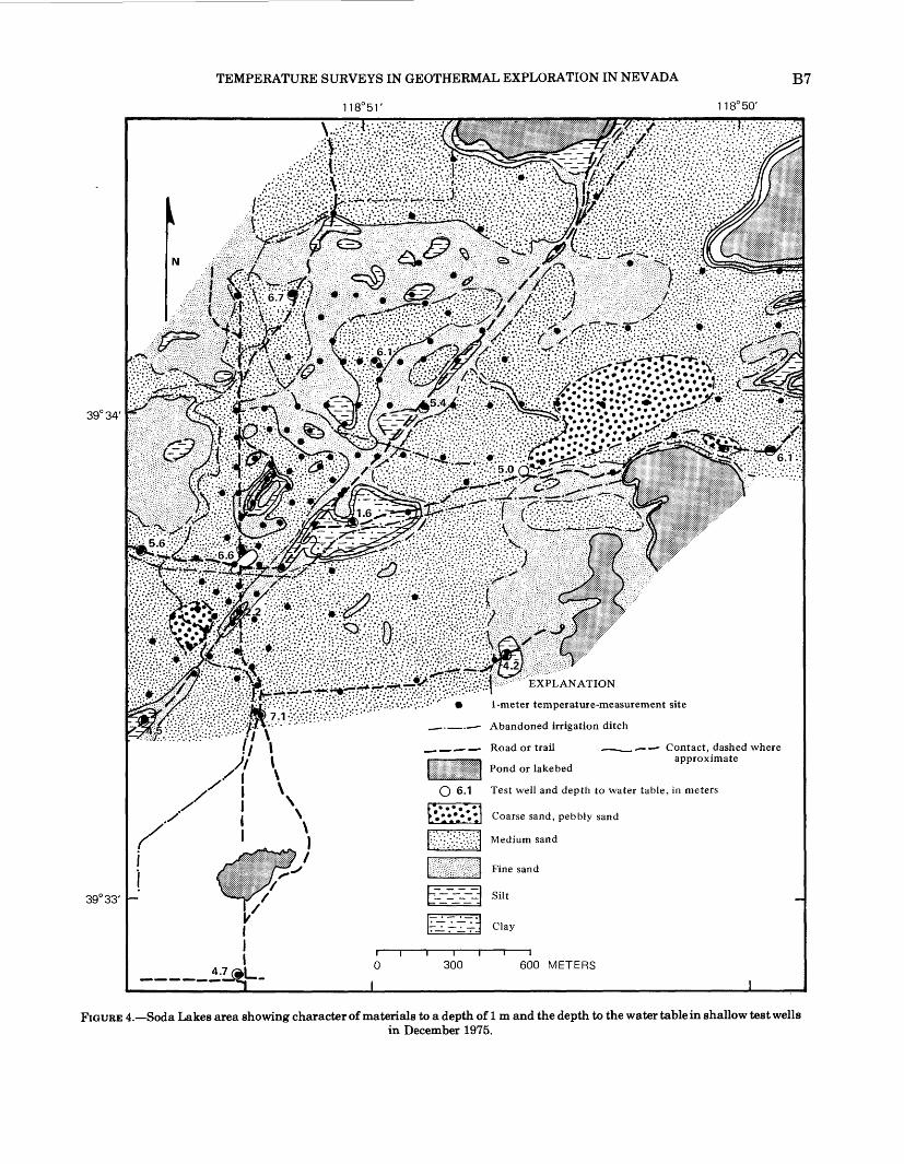
4. Map of Soda Lakes area showing character of materials to a depth of 1 m and the depth to the water table in shallowtest wells in December 1975 ..................................................................................................... . .... ....- ................................ 7
5. Map showing temperature at a depth of 1 m near steam well, November 23, 1973 .............................................................. 96. Map of Soda Lakes area showing temperature at a depth of 30 m, fall 1973 .......................................................................... 107. Map of Soda Lakes area showing temperature at a depth of 1 m on November 23,1973 and area of snowmelt in
January 1974 ..........................................................................._ 118. Map of Soda Lakes area showing density of Russian thistle on February 5, 1974 ................................................................ 139. Map of Soda Lakes area showing temperature at a depth of 1 m on June 15 and September 20,1974 .......................... 14
10. Fluctuations in temperature at a depth of 1 m at three sites in Soda Lakes area compared with fluctuations in airtemperature at Fallen Experiment Station during 1975 .......................................................................................................... 15
11. Correlation of temperatures at a depth of 20 m with temperatures at a depth of 1 m in Soda Lakes area,September 1974 ............................................................... 17
12. Topographic map of Upsal Hogback area showing depth to the water table in test wells, configuration of the watertable, and direction of shallow ground-water movement in July 1975 ................................................................................ 18
13. Map of Upsal Hogback area showing temperature at a depth of 1 m, June 1975 .................................................................. 1914. Map of Upsal Hogback area showing temperature at a depth of 1 m, October 29, 1975 ...................................................... 2015. Map of Upsal Hogback area showing temperature at a depth of 1 m, December 2, 1975 .................................................... 2216. Map of Upsal Hogback area showing temperature in test wells at a depth of 30 m, September 1975 ............................ 2317. Correlation of temperature at a depth of 30 m with temperature at a depth of 1 m in Upsal Hogback area,
December 1975 ............................................................. 24
III

IV CONTENTS
TABLEPage
TABLE 1. Characteristics of idealized temperature waves at a depth of 1 m in western Carson Desert ............................................ B3
GEOHYDROLOGY OF GEOTHERMAL SYSTEMS
USE OF TEMPERATURE SURVEYS AT A DEPTH OF 1 METER IN GEOTHERMAL EXPLORATION IN NEVADA
By F. H. OLMSTED
ABSTRACT
Temperature surveys at a depth of 1 m in the Soda Lakes and Upsal Hogback areas of the western Carson Desert, Nevada, had varying degrees of success in delineating temperature and heat- flow anomalies at greater depths. Optimum results were obtained in a detailed survey of a small area near a f umarole and an aban doned steam well in the Soda Lakes area. At this location steam occurs above the water table and the unconfined water is at the boiling temperature at depths of only a few meters; also tempera tures and heat flows are far above background values. Somewhat more equivocal results were obtained in surveys of a larger sur rounding area in which the temperature range at 1 m was smaller than immediately adjacent to the fumarole and steam well, and in which perturbing effects of geologic, topographic, hydrologic, and other factors not related directly to geothermal heat flow are locally significant. Poorest results were obtained in surveys of the Upsal Hogback area, where temperature of the thermal water leaking into shallow aquifers is much less than that in the Soda Lakes area, the range in temperature at a depth of 1 m is corres pondingly smaller, and the variability of the geology, topography, depth to the water table, and other perturbing factors is greater than that in the Soda Lakes area.
INTRODUCTION
In principle, temperature surveys at depths as shallow as 1 or 2 m could be used to delineate deeper thermal anomalies or areas of high geothermal heat flow, provided that temperature differences caused by extraneous factors were not so large as to mask the temperature differences caused by variations in heat flow. Some extraneous factors that affect shallow temperatures are local variations in the character and moisture content of the near-surface materials, topography, depth to the water table, vegetation, land use, and microclimate. The princi pal advantage of temperature measurements at such shallow depths in comparison with deeper meas urements is their relatively low cost in both time and money.
Earlier investigators have reported both failure and success using shallow temperature surveys in geothermal exploration. In reviewing evidence from
a study of shallow temperature gradients in relation to anomalously high heat flow caused by oxidizing ore bodies, Levering and Goode (1963, p. 39) concluded that temperature measurements at depths of only 1 or 2 m were useless in detecting abnormal geothermal gradients at greater depths. Kappel- meyer (1957, p. 248-254) reached similar conclusions about the use of such measurements to find buried horsts, salt domes, or local concentrations of radio active material, although he believed it possible in principle to outline areas underlain by fissures carrying thermal water upward into the shallow ground-water system. Kintzinger (1956), in fact, reported the successful use of 1-m temperature measurements in outlining an area near Lordsburg, N.M., underlain by hot ground water encountered in wells at depths of only 20-25 m.
The present paper (1) briefly reviews the theoretical difficulties and limitations of temperature measure ments at 1 m depth in determining geothermal heat flow; (2) presents the results of field tests of the method at two geothermal anomalies in west-central Nevada, where fairly abundant comparative tem perature data are available at depths below the zone affected by fluctuations in solar energy; and (3) evaluates the general applicability of the method in similar geologic, hydrologic, and climatic settings.
THEORETICAL CONSIDERATIONS
If it were possible to make sufficient measure ments to define average annual temperature at the land surface and at a depth of 1 m, the temperature at 1 m would be found to exceed that at the land surface, assuming the climate was not changing and heat transfer toward the surface was by conduction. The temperature difference in a horizontal uniform layer would be expressed as
10K
Bl
B2 GEOHYDROLOGY OF GEOTHERMAL SYSTEMS
10 20 30 40 50 6012
S 10 uV)UJ UJcc oUJQ
~ 8
O
o
O CCu.UJccD
< ocUJ0.2UJH
12
10
10 20 30 40
HEAT FLOW, IN HEAT-FLOW UNITS
50 60
K=Thermal conductivity,in millicalories per centimeter • degree • second
FIGURE 1. Difference in average annual temperature between land surface and a depth of 1 m in relation to thermal conductivity and geothermal heat flow.
where AT^-i is the temperature difference from land surface to a depth of 1 m, in degrees Celsius; Q is the geothermal heat flow (heat-flux density), in micro- calories per square centimeter per second (y cal»cnv2 s-1 ); and K is the thermal conductivity of the layer, in millicalories per centimeter per degree per second (mcal»cm1.°C'1»s-1 ). In an area of so-called "normal" geothermal heat flow about 1 ycal-cm.-2^ 1 or 1 HFU (heat-flow unit) the temperature difference in material having a thermal conductivity of 2 meal* cm- 1»°C- 1»s-1 would be only 0.05°C, which is barely within the range detectable by ordinary temperature- measuring equipment.
Temperature differences from land surface to a depth of 1 m for values of heat flow and thermal
conductivity representative of conditions in geo thermal areas in west-central Nevada are shown in figure 1. A K (thermal conductivity) of 0.5 mcakcnv1 °C'1»s-1 would be typical of dry silt or fine sand; a K of 4 mcal»cm -1»°C' 1»s-1 would be typical of wet coarse sand. Where the thermal conductivity is large, the temperature difference from 0 to 1 m is small, even for a heat flow of 100 times "normal." Low thermal conductivity, on the other hand, is associated with a large temperature difference (fig. 1).
For the simple case just described, if sufficient measurements could be made to define the average annual temperature at 1 m, the only problems in relating temperature at 1 m to geothermal heat flow would be variations in thermal conductivity with
TEMPERATURE SURVEYS IN GEOTHERMAL EXPLORATION IN NEVADA
TABLE 1. Characteristics of idealized temperature waves at a depth of 1 m in western Carson Desert
B3
Kind of wave
"Weather" ..............................Seasonal ..................................
Period(days)
1
10365
Amplitude at surface (°C)
15.0 4.0
15.0
Amplitude at 1 m depth (°C)
<x = 1.5 x lO^cm2^1
2.6 x 10⁻⁶ 0.029 6.65
a. = 6.0 x 10⁻³cm2s'1
6.2 x 10⁻³ 0.34 9.98
Timelag (days)
Oi = 1.5 x 10~3cm2 s~
2.467.8
47.4
1 a. = 6.0 x lO-ocmV 1
1.23 3.9
23.7
both place and time and variations with place in average annual temperature at the land surface. Variations in thermal conductivity are troublesome where the near-surface materials in the area of investigation are not uniform. Variations in average annual temperature are difficult to deal with where topography is irregular and vegetative cover is variable. As shown in figure 1, heat-flow differences of several tens of heat flow units could be masked completely by moderate variations in thermal conductivity or by differences in average annual temperature at the surface of only a few degrees Celsius. In spite of these potential problems, measurement of average annual temperatures at 1 m could be a powerful tool in geothermal prospecting if the area selected for study were fairly level and had uniform soils, vegetation, and land-use patterns.
The accurate determination of average annual temperatures at 1 m would require several sets of synoptic measurements during the year, such as at monthly intervals. However, because of this require ment, much of the advantage of 1-m temperature surveying over surveys at greater depth but at fewer sites is lost. Therefore, it is desirable to consider the advantages and disadvantages in using a single set of synoptic measurements at 1-m depth.
The principal advantages of a single set of measurements are the savings in time and expense and the prompt availability of the results for use in interpretation and decisionmaking in further ex ploration. The chief disadvantage is that, in dealing with a single set of synoptic measurements, another group of variables enters the problem: the areal variations in temperature related to differences in soil-temperature response to periodic and non- periodic fluctuations in solar-energy input.
Although diurnal temperature waves are damped to amplitudes too small to be measured at 1 m in most climatic and geologic environments, fluctuations having longer periods, including the annual tem perature wave, have significant amplitude at 1 m depth. In the simple case of a single homogeneous soil or rock layer of semi-infinite extent, the response at the base of the layer to harmonic fluctuations in temperature (sinusoidal waves) at the top surface or
land surface can be expressed by two equations:
(1)
(2)
where Ax is the amplitude of the temperature waveat the base of layer x (°C),
A 0 is the amplitude of the temperature waveat the land surface (°C),
x is the thickness of layer x (cm), a is the thermal diffusivity of layer x (cm2
s-1 ), P is the period of the temperature wave (s),
andtx - t0 is the time lag between the temperature
waves at the land surface and at the base of layer x (s).
As shown by equations (1) and (2), the amplitude of a temperature wave decreases exponentially with a linear increase in depth, but the timelag increases linearly with a linear increase in depth. The longer the period of the wave at the surface, the greater will be the amplitude of that wave at any given depth.
In general, temperature waves at the land surface, which are caused by fluctuations in solar-energy input, may be grouped in three categories on the basis of their periods: (1) diurnal, (2) "weather," and (3) annual (or seasonal) waves. The periods of the first and third categories are indicated by their names and are regular. Waves of the second category are irregular in period and are caused by the passage of air masses of different meteorological character istics.
Features typical of each of the three types of waves in the area of study, in west-central Nevada, are presented in table 1. The simple case of idealized harmonic temperature waves being damped con- ductively in a semi-infinite uniform medium is assumed. The two values of thermal diffusivity shown represent the approximate upper and lower limits found in the area of study. The periods and
B4 GEOHYDROLOGY OF GEOTHERMAL SYSTEMS
- -10
-15 -15JAN FEB MAR APR MAY JUN JUL AUG SEP OCT NOV DEC
©A ) Temperature at land surface. Wave amplitude=15°C
Temperature at 1 m, thermal diffusivity 6.0 x 10~ 3 cm 2 s" 1 . Wave amplitude=10.0°C, timelag=23.7 days
(CJ Temperature at 1 m, thermal diffusivity ^"^ 1.5 x IQr'cm^s" 1 . Wave amplitude2
6.6° C; time lag =47.4 days
FIGURE 2. Idealized annual temperature fluctuations at land surface and a depth of 1 m for approximate conditionswestern Carson Desert area, Nevada.
amplitudes of the waves at the land surface likewise are typical of conditions in west-central Nevada.
Stratification of near-surface materials produces effects on the temperature waves which may differ substantially from the effects in the uniform medium described above. Lachenbruch (1959) and Van Wijk and Derksen (1966, p. 177-180) have shown that the amplitude of a temperature wave at a given depth in a multilayered medium can range from several times smaller to somewhat larger than that in a single layer, depending.on the relative thermal properties, especially thermal inertia (contact coefficient), of the layers.
As stated earlier, the amplitude of the diurnal waves is too small to be measured in the range of conditions likely to be found in the study area. Although detectable with ordinary temperature- measuring equipment, the amplitude of the "weather" waves is not large enough to be a troublesome factor. The chief problems are associated with the long- period annual waves, where differences in thermal diffusivity can result in differences in phase-lag time of several weeks and differences in amplitude of
more than 2°C from place to place. (See table 1 and fig. 2.) Owing to the combined effects of the differences in amplitude and timelag, the variations in temperature at 1 m from place to place exceed 4°C in midwinter and midsummer (fig. 2). Stratification, described above, can cause even larger differences. As shown in figure 2, these differences could be minimized by making the temperature surveys in early April or early October.
Although the difficulties described above appear formidable, they are only part of the entire problem. Other significant factors causing variations in temperature at 1 m not related to geothermal heat flow include variations in convective heat transport by water, vapor, and air, and variations resulting from areal variations in the solar-air-earth heat budget, such as the effects of topography, albedo, surface emissivity, wind, and vegetation. These factors could cause perturbations as large as those caused by the areal variations in thermal diffusivity and stratification. Added to these difficulties are the variations in thermal diffusivity with time as the moisture content of the near-surface materials
TEMPERATURE SURVEYS IN GEOTHERMAL EXPLORATION IN NEVADA B5
changes in response to precipitation and other weather factors. Clearly, there are serious obstacles to the successful use of synoptic temperature surveys at 1 m depth to determine geothermal heat-flow or temperature anomalies at depths below the range of solar-energy fluctuations. In spite of these obstacles, however, a practical test of the technique was believed warranted.
EQUIPMENT AND METHODOLOGY
Temperature measurements were made with a two- bead thermistor mounted at the tip of an aluminum probe 1 m in length, connected by a 3-conductor cable to a solid-state Wheatstone bridge having a digital readout. Temperature was recorded to the nearest 0.01 °C. Frequent calibration checks with a mercury- glass thermometer indicated an accuracy of about ±0.3°C for individual measurements.
In soft coherent deposits, such as damp silt or clay, access holes were driven by hand with a light-weight steel driver. Most of the holes, in sandy deposits, were made with a soil auger 57 mm in diameter, lithologic character and moisture content of mate rials were recorded at each site.
After insertion of the temperature probe into the material at the bottom of the access hole, readings were made at regular time intervals and equilibrium temperature was computed by a method of extrapola tion to infinite time described by Parasnis (1971).
FIELD APPLICATION IN SODA LAKES AREA
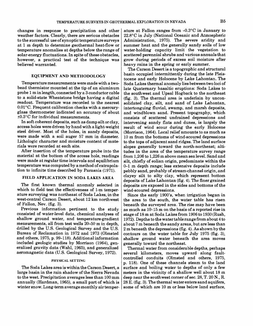
The first known thermal anomaly selected in which to field test the effectiveness of 1-m temper ature surveying was northeast of Soda Lakes, in the west-central Carson Desert, about 12 km northwest of Fallen, Nev. (fig. 3).
Previous information pertinent to the study consisted of water-level data, chemical analyses of shallow ground water, and temperature-gradient measurements, all from test wells 20-50 m in depth, drilled by the U.S. Geological Survey and the U.S. Bureau of Reclamation in 1972 and 1973 (Olmsted and others, 1975, p. 99-118). Additional information included geologic studies by Morrison (1964), gen eralized gravity data (Wahl, 1965), and generalized aeromagnetic data (U.S. Geological Survey, 1972).
PHYSICAL SETTING
The Soda Lakes area is within the Carson Desert, a large basin in the rain shadow of the Sierra Nevada to the west. Precipitation averages less than 100 mm annually (Hardman, 1965), a small part of which is winter snow. Long-term average monthly air temper
ature at Fallen ranges from -0.3° C in January to 22.8°C in July (National Oceanic and Atmospheric Administration, 1975). The severe aridity and summer heat and the generally sandy soils of low water-holding capacity limit the vegetation to scattered perennial shrubs and various annuals that grow during periods of excess soil moisture after heavy rains in the spring or early summer.
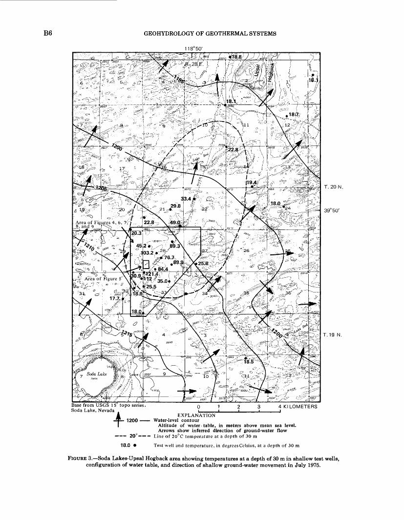
The Carson Desert is a topographic and structural basin occupied intermittently during the late Pleis tocene and early Holocene by Lake Lahontan. The Soda Lakes thermal anomaly lies between two loci of late Quaternary basaltic eruptions: Soda Lakes to the southwest and Upsal Hogback to the northeast (fig. 3). The thermal area is underlain by uncon- solidated clay, silt, and sand of Lake Lahontan, intertonguing fluvial, swamp, and marsh deposits, and windblown sand. Present topography, which consists of scattered undrained depressions and intervening sandy flats and dunes, is largely the result of wind scour during the early Holocene (Morrison, 1964). Local relief amounts to as much as 10 m from the bottoms of wind-scoured depressions to the tops of adjacent sand ridges. The land surface slopes generally toward the north-northeast; alti tudes in the area of the temperature survey range from 1,206 to 1,226 m above mean sea level. Sand and silt, chiefly of eolian origin, predominate within the 0-1 m depth range; less extensive deposits include pebbly sand, probably of stream-channel origin, and clayey silt to silty clay, which represent bottom deposits of Lake Lahontan (fig. 4). The finer grained deposits are exposed in the sides and bottoms of the wind-scoured depressions.
Since the early 1900's, when irrigation began in the area to the south, the water table has risen beneath the surveyed area. The rise may have been as much as 10-15 m on the basis of a reported rise in stage of 18 m at Soda Lakes from 1906 to 1930 (Rush, 1972). Depths to the water table range from about 4 to about 7 m beneath the sandy areas, but are less than 2 m beneath the depressions (fig. 4). As shown by the contours on the water table for July 1975 (fig. 3), shallow ground water beneath the area moves generally toward the northeast.
Thermal water from considerable depths, perhaps several kilometers, moves upward along fault- controlled conduits (Olmsted and others, 1975, p. 118). One of these channels steam to the land surface and boiling water to depths of only a few meters in the vicinity of a shallow well about 18 m deep near the southwest corner of sec. 28, T. 20 N., R. 28 E. (fig. 3). The thermal water enters sand aquifers, some of which are 10 m or less below land surface,
B6 GEOHYDROLOGY OF GEOTHERMAL SYSTEMS
118° 50'
T.20N.
39°50'
r- T.19 N.
Base from USGS 15 topo series. Soda Lake, Nevada
EXPLANATION 1200 —- Water-level contour
Altitude of water-table, in meters above mean sea level. Arrows show inferred direction of ground-water flow
•——— 20 —— — Line of 20° C temperature at a depth of 30 m
18.0 Test well and temperature, in degrees Celsius, at a depth of 30 m
FIGURE 3.—Soda Lakes-Upsal Hogback area showing temperatures at a depth of 30 m in shallow test wells, configuration of water table, and direction of shallow ground-water movement in July 1975.
TEMPERATURE SURVEYS IN GEOTHERMAL EXPLORATION IN NEVADA BY118° 50'
39°34'
^^^^^isSM^^^UK^^^^Mi^^^iM^i^K
39° 33'
^-— Contact, dashed where approximate
EXPLANATION
-meter temperature-measurement site
Abandoned irrigation ditch
_._—.—- Road or trail -
Pond or lakebed
Test well and depth to water table, in meters
Coarse sand, pebbly sand
Medium sand
Fine sand
>r-£i-r- SiltfZfZ4-i Clay
300 600 METERS
FIGURE 4.—Soda Lakes area showing character of materials to a depth of 1 m and the depth to the water table in shallow test wellsin December 1975.
B8 GEOHYDROLOGY OF GEOTHERMAL SYSTEMS
through which it moves laterally toward the north east. The temperature anomaly thus produced is strongly asymmetrical toward the northeast (fig 3).
TEMPERATURE SURVEY IN VICINITY OF STEAM WELL
The first temperature measurements at 1-m depth were made during November 1973 in the vicinity of an abandoned well, reported to have been originally about 18 m deep, near the southwest corner of sec. 28, T. 20 N., R. 28 E. (fig. 3). The site was selected because of suspected high near-surface temperatures. Evi dence for a shallow thermal anomaly consisted of hydrothermal alteration of the sandy eolian deposits to kaolinite and iron hydroxides and oxides, steam issuing from the old well and from a nearby fumarole, and observed rapid snowmelt in an area coextensive with the exposures of hydrothermally altered deposits. Lateral spacing of the temperature- measurement sites ranges from about 5 m in the zone of highest temperature near the fumarole and steam well to more than 100 m on the margins of the strongest thermal anomaly, where temperatures at 1 m were less than 30°C (fig. 5).
Temperature at 1 m ranged from less than 30°C to more than 90°C in a small linear band trending northeast and centered on the fumarole (fig. 5). Highest temperatures were associated with the area of most intense hydrothermal alteration and prob ably indicate the presence of steam near the surface. The temperature pattern suggests rising thermal water along a northeast-trending elongate or linear conduit, probably fault-controlled. Possible presence of a linear zone approximately perpendicular to the main zone is indicated by the temperature pattern 30- 50 m northeast of the steam well.
The high temperatures probably result in large part from heat transport by steam rising from a boiling water table rather than chiefly by heat conduction through the altered clayey sediments above the water table. Depth to the water table within the area shown in figure 5 has not been measured, but measurements in nearby test wells indicate probable depths of 5-7 m outside the hottest part of the thermal anomaly.
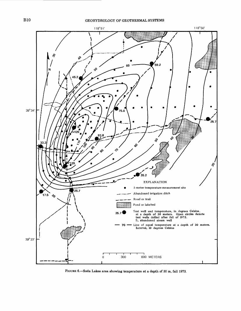
TEMPERATURE SURVEY IN NOVEMBER 1973
Concurrently with the temperature survey of the small area adjacent to the old steam well, measure ments were made in a much larger surrounding area. Earlier data from test wells ranging in depth from 9 to 44 m indicated an asymmetrical northeast- trending thermal anomaly centered approximately at the steam well (fig. 6). Temperature at a depth of 30
m below land surface ranged from an inferred temperature of more than 120°C near the steam well—boiling temperature at hydrostatic pressure— to less than 20°C on the margins of the anomaly. Lateral temperature gradient toward the southwest was greater than that toward the northeast, and gradients along the northwest margin were greater than those along the southeast margin.
With a range in temperature of more than 100° C at 30 m, it was anticipated that the temperature pattern at 1 m would reflect deeper temperatures and that, with much greater density of measurement sites, the temperature pattern at 1 m might reveal features not apparent from the data at 30 m shown in figure 6.
Because of concurrent other work, it was not possible to complete the measurements at about 100 sites within a few days, as would have been desir able. Instead, the survey required nearly a month, from November 11 to December 7, 1973. Because temperature at 1 m changed considerably during this period, the temperature at each site was adjusted to a midperiod date of November 23 on the basis of repeated measurements at several sites. A linear rate of change of temperature during the period of measurements was assumed, and the same rate of change was used for all sites. Analysis of air- temperature data for the nearby weather station atFallen suggests that the actual change in tempera ture in the ground probably was irregular, in response to antecedent "weather" cycles, as dis cussed previously. Moreover, variations probably existed in the rate of temperature change from place to place, owing to both areal and temporal variations in thermal diffusivity. However, the differences between the interpolated temperatures used and the actual values are believed to be small—on the order of a few tenths of a degree Celsius at most sites.
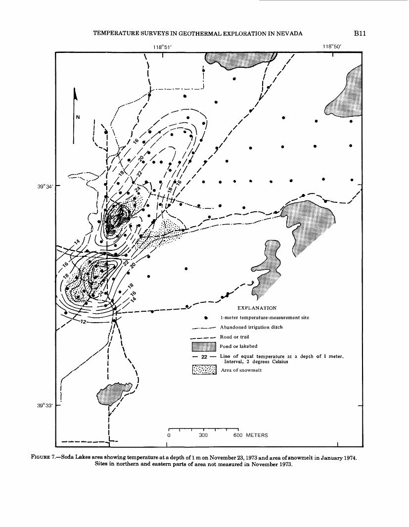
Results of the temperature survey are shown in figure 7. Temperature on the margins of the anomaly, presumably where the geothermal heat flow is normal or nearly normal, was about 12°C; temperature in the warmest parts of the anomaly exceeded 90° C near the steam well and 30° C at another thermal high about 500 m south of the steam well. The general northeasterly alinement of the long axis and the asymmetry of the anomaly are similar to the temperature pattern at 30 m (compare figs. 6 and 7). However, a significant difference is revealed by the greater density of the 1 m data: instead of one thermal maximum centered at the steam well, there were two en echelon elongate maxima, separated by a lower temperature trough, all oriented northeast. The zone of highest temperature northeast of the steam well, where the temperature exceeded 20°C,
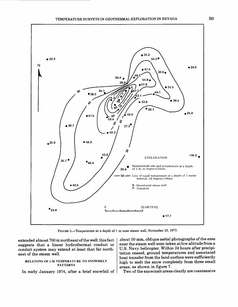
TEMPERATURE SURVEYS IN GEOTHERMAL EXPLORATION IN NEVADA B9
• 22.3
N • 26.9
• 24.6
,25.9
EXPLANATION>16.3
0 Measurement site and temperature at a depth 26.9 of 1 m, in degrees Celsius
50 Line of equal temperature at a depth of 1 meter Interval, 10 degrees Celsius
S: Abandoned steam well F: Fumarole
24.850 METERS
• 17.7
FIGURE 5.—Temperature at a depth of 1 m near steam well, November 23, 1973.
extended almost 700 m northeast of the well; this fact suggests that a linear hydrothermal conduit or conduit system may extend at least that far north east of the steam well.
RELATONS OF 1-M TEMPERATURE TO SNOWMELT PATTERNS
In early January 1974, after a brief snowfall of
about 50 mm, oblique aerial photographs of the area near the steam well were taken at low altitude from a U.S. Navy helicopter. Within 24 hours after precipi tation ceased, ground temperatures and associated heat transfer from the land surface were sufficiently high to melt the snow completely from three small areas, as shown in figure 7.
Two of the snowmelt areas clearly are coextensive
BIO GEOHYDROLOGY OF GEOTHERMAL SYSTEMS
118°5T118° 50'
39° 34'
39° 33'
EXPLANATION
• 1-meter temperature-measurement site
___.—.—- Abandoned irrigation ditch
__._ —. —- Road or trail
Pond or lakebed
25.7 (
70
Test well and temperature, in degrees Celsius, at a depth of 30 meters. Open circles denote test wells drilled after fall of 1973. S, abandoned steam well
Line of equal temperature at a depth of 30 meters. Interval, 10 degrees Celsius
300 600 METERS
FIGURE 6.—Soda Lakes area showing temperature at a depth of 30 m, fall 1973.
TEMPERATURE SURVEYS IN GEOTHERMAL EXPLORATION IN NEVADA Bll118° 50'
39°34'
39° 33'
7Y(l|f%fel^'
S EXPLANATION
• 1-meter temperature-measurement site
___.—.—- Abandoned irrigation ditch
_.._ —. —- Road or trail
Pond or lakebed
— 22 '— Line of equal temperature at a depth of I meterInterval, 2 degrees Celsius
Area of snowmelt
300 600 METERS
FIGURE 7.—Soda Lakes area showing temperature at a depth of 1 m on November 23,1973 and area of snowmelt in January 1974. Sites in northern and eastern parts of area not measured in November 1973.
B12 GEOHYDROLOGY OF GEOTHERMAL SYSTEMS
with thermal maxima at 1 m as shown by the November 23, 1973 data, but a third area, on the southeast flank of the principal thermal anomaly, seems not to be related directly to the temperature pattern. However, comparison with the near-surface lithology and the depth to water (fig. 4) suggests that the third snowmelt area indicates a heat sink coincident with a wind-scoured depression. The near- surface deposits in the depression are chiefly clay and silt of low thermal diffusivity in comparison with that of the damp sand of the surrounding area. Moreover, the depth to a warm water table is less than 2 m in the depression, as compared to a depth of more than 5 m in the surrounding higher, sandy area.
RELATIONS OF 1-M TEMPERATURES TO GROWTH OF RUSSIAN THISTLE
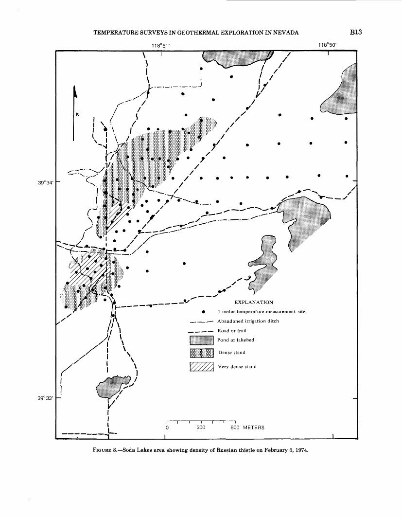
Color vertical aerial photographs taken in February 1974 revealed brown color patterns which were approximately coextensive with the areas of maximum temperature at 1 m depth in November 1973 (fig. 8). Later inspection on the ground indicated that the brown patterns were caused by dense stands of dried-up Russian thistle (Salsola Kali L. var. tenufolia Fausch). The thistle appears to thrive in sandy soil, and the density and vigor of the stands correlate directly with the ground temperature (fig- 8).
TEMPERATURE SURVEYS IN JUNE AND SEPTEMBER 1974
In order to determine whether the configuration and extent of the 1-m anomaly changes with time, a survey was made northeast of the steam well in June 1974, and areal coverage was extended beyond that of the November 1973 survey, mostly toward the east and northeast, in September 1974.
The June measurements indicated a pattern similar to that of the previous November, but with minor differences, probably related to areal varia tions in thermal diffusivity of the shallow materials. (Compare figs. 7 and 9.) The September 1974 measurements showed that the thermal anomaly at 1-m depth extended more than 2 km east and northeast of the center of the November 1973 anomaly. A similar pattern at 30 m was established on the basis of extrapolated temperature gradients from measurements in 20-m-deep test wells drilled in October 1974.ANNUAL FLUCTUATION IN TEMPERATURE AT THREE SITES
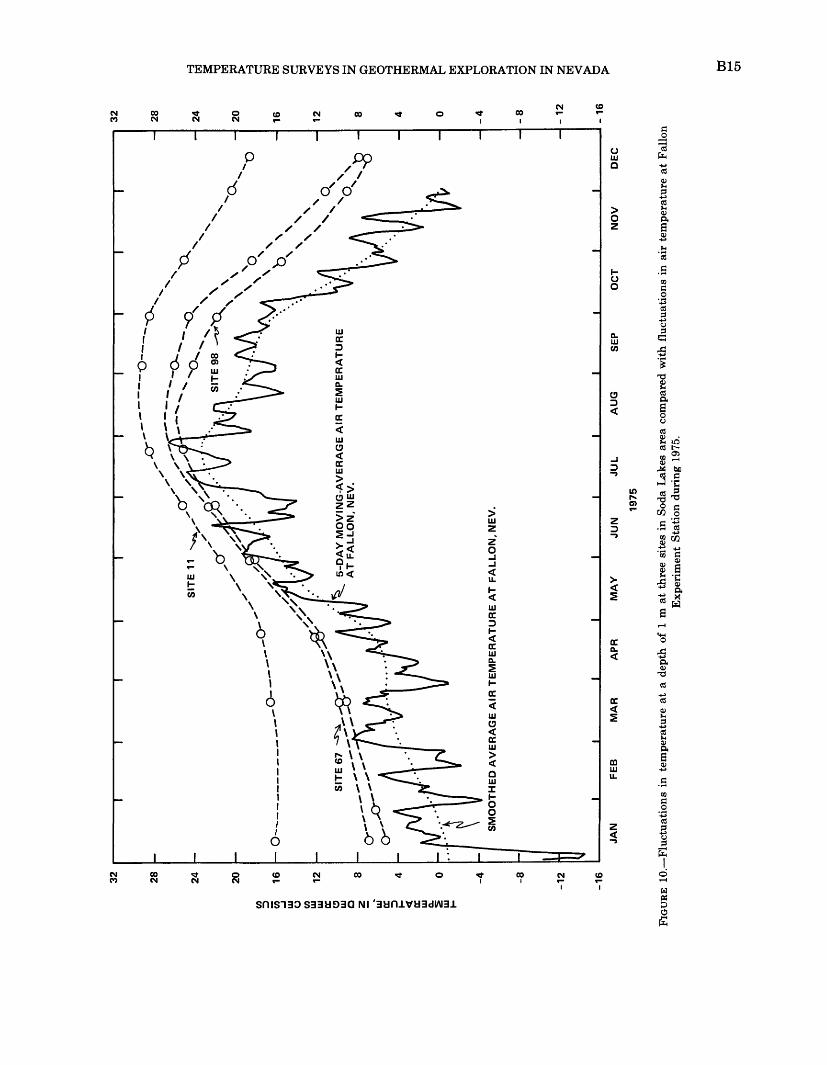
Monthly temperature measurements during 1975 were made at three sites in order to determine differences in the nature of the annual temperature
wave in three different lithologic and thermal environments. The sites (fig. 9) were selected to represent the approximate range of temperature fluctuations throughout the surveyed area. Site 98, south of the thermal anomaly, is in sand of chiefly eolian origin. Depth to the water table averaged about 4.7 m in 1975. Site 67, also in predominantly sandy deposits but containing slightly more clay and silt than at site 98, is on the northwest flank of the anomaly. Depth to water averaged about 6.7 m in 1975. Site 11, about 380 m southeast of the steam well, is near the north edge of the depression where snowmelt was observed in January 1974, as de scribed earlier. The deposits at site 11 are lacustrine clay and silt having a moisture content greater than that at the other two sites.
As shown in figure 10, temperature at all three sites was always higher than the smoothed-average air temperature at Fallon Experiment Station; the amplitude of the annual temperature fluctuations was less at the three sites than at Fallon; and the temperature waves at the three soil sites lagged the annual air temperature wave at Fallon, as would be expected from theoretical considerations.
Differences among the three sites are apparent in figure 10. The temperature at site 11, the hottest location, differs from that at site 98, the coldest location, by amounts ranging from 3°C in late spring to about 11°C in early winter. The temperature difference between sites 67 and 98 ranges from less than 0.5°C in the spring to about 3°C in the fall. These temperature differences are largely the result of differences in thermal diffusivity at the three sites but are also related to differences in surface conditions and to the effect of a shallow water table at site 11. During most of the year, the thermal diffusivity of the damp clay and silt at site 11 was less than that of the sandier materials at the other two sites; this relation accounts in part for the smaller amplitude of the annual temperature wave at site 11. The smaller amplitude at site 11 probably is also caused by stratification and heat-sink effects of a warm, shallow water table. The range in temperature differences among the three sites during the year illustrates the danger of using synoptic temperature measurements at only one time during the annual cycle in trying to discern patterns related to variations in geothermal heat flow.
CORRELATION OF TEMPERATURES AT DEPTHS OF 1 METER AND 20 METERS
The evidence discussed above suggests that, in the Soda Lakes area, a temperature survey at a depth of 1 m might provide a fairly reliable indication of the
TEMPERATURE SURVEYS IN GEOTHERMAL EXPLORATION IN NEVADA B13118° 50'
39°34'
39° 33'
EXPLANATION
1-meter temperature-measurement site
Abandoned irrigation ditch
_._—.—- Road or trail
Pond or lakebed
Dense stand
Very dense stand
300 600 METERS
FIGURE 8.—Soda Lakes area showing density of Russian thistle on February 5, 1974.

B14 GEOHYDROLOGY OF GEOTHERMAL SYSTEMS
118° 50'
39°34'
- --
39° 33'
EXPLANATION
• 1-meter temperature-measurement site
__-.——— Abandoned irrigation ditch
_. _ — —- Road or trail
Pond or lakebed
— 32 — Lines of equal temperature at a depth of I meter. Interval, 2 degrees Celsius. Solid lines represent
•••28 ••• temperature on September 20, 1974; dotted lines on June 15, 1974
O 98 Site of periodic temperature measurements at a depth of 1 meter during 1975
300 600 METERS
FIGURE 9.—Soda Lakes area showing temperature at a depth of 1 m on June 15 and September 20, 1974.
32 28 24 20
CO 33 16
ui u CO ui 12
QJ
It
cc u UI 0
-4 -8 -12
-16
- O
5-D
AY
MO
VIN
G-A
VE
RA
GE
AIR
TE
MP
ER
AT
UR
E
AT
FA
LL
ON
, N
EV
.
SM
OO
THE
D A
VE
RA
GE
AIR
TE
MP
ER
AT
UR
E A
T F
AL
LO
N, N
EV
.
I
32 28 24 20 16 12 -4 -8 -12
-16
a M I 03
i—i
SI
O w O H ffi X a O 2
JAN
FEB
M
AR
A
PR
M
AY
JUN
JU
L A
UG
1975
SEP
OC
T N
OV
D
EC
FIGU
RE 1
0.—
Fluc
tuat
ions
in
tem
pera
ture
at
a de
pth
of 1
m a
t th
ree
site
s in
Sod
a La
kes
area
com
pare
d w
ith f
luct
uatio
ns i
n ai
r te
mpe
ratu
re a
t Fa
llon
Exp
erim
ent
Stat
ion
duri
ng 1
975.
W
i—'
en
B16 GEOHYDROLOGY OF GEOTHERMAL SYSTEMS
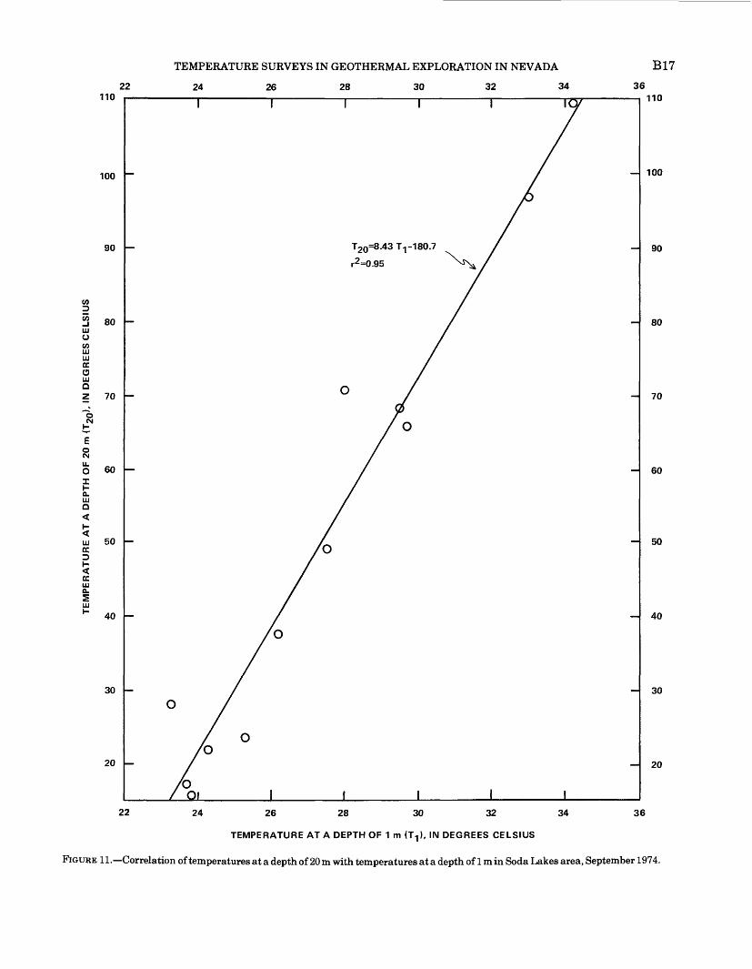
extent and configuration of a thermal anomaly at greater depths, below the range of influence of the annual weather cycle. A simple test of the reliability of a temperature survey at 1 m is a correlation of temperature at 1 m with temperature at 20 m at test- well sites where the deeper temperature data are available (fig. 11). The least-mean-squares linear- regression equation is
720 = 8.43 TI - 180.7where T2Q is temperature at 20 m and TI is temperature at 1 m in September 1974. The coefficient of determination, r 2 (a measure of variance), is 0.95, which indicates a fairly good fit to the least-mean-squares regression over a temper ature range of nearly 100°C at 20 m and 11°C at 1 m. However, at temperatures less than 40°C at 20 m, the scatter of the data indicates a much poorer corre lation in that temperature range.
FIELD APPLICATION IN UPSAL HOGBACK AREA
The second area studied was near Upsal Hogback, a group of low basalt cinder cones or tuff rings about 12-16 km north-northeast of Soda Lake.
Previous information for the Upsal Hogback area was similar to that for the Soda Lakes area, except that shallow test drilling near the Hogback began about the same time as the 1-m temperature survey instead of preceding it.
GEOLOGY AND TOPOGRAPHY
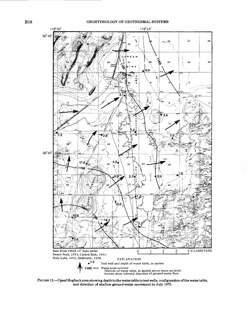
The basalt cones or tuff rings of the Upsal Hogback were formed by intermittent eruptions, chiefly during an interpluvial time in the late Pleistocene when Lake Lahontan either was dry or stood at a level below the site of the eruptions (Morrison, 1964, p. 100). The cones are probably along a concealed fault or fault system which also intersects the Soda Lakes to the south-southwest. Near the Hogback, the post-Lake Lahontan blanket of sandy deposits that characterizes much of the Soda Lakes area consists only of scattered dunes in the north-central and eastern parts of the area. In contrast, sands and clays of Lake Lahontan, now eroded by both wind and water, crop out on the flanks of the Hogback. The land surface is character ized by a large contrast in albedo, from dark surfaces with a lag of basalt gravel to light exposures of lacustrine clay and silt. The largely bare, flat surface of Carson Sink, the sump for all the drainage in the region, extends into the northeast part of the area. Land-surface altitudes range from 1,270 m at the top of a cone near the south end of the Hogback to 1,178 m in the Carson Sink (fig. 12).
DEPTH TO WATER AND GROUND-WATER MOVEMENT
Depth to the water table in July 1975 ranged from less than 1 m in the Carson Sink and adjacent low, flat areas to about 20 m on the margins of Upsal Hogback. The range in depth was considerably greater than that in the Soda Lakes area and, together with the greater topographic relief and the greater contrast in albedo, presented potential problems for the application of the 1-m temperature- survey method.
The general direction of ground-water movement, perpendicular to the water-table contours, is north ward to eastward, toward the Carson Sink (fig. 12). The vertical component of ground-water movement is generally upward; the upward gradient increases toward the Carson Sink. However, on the flanks of Upsal Hogback, the upward gradient is small to zero, and at one site on the southwest side of the Hogback, the gradient is downward.
TEMPERATURE SURVEY ON JUNE 15, 1975
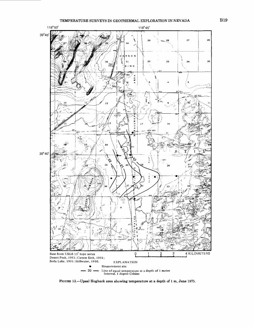
Temperature was measured at 1 m on June 15, 1975, at the time the drilling of several test wells 30-50 m deep was started north and east of the Hogback. One of the wells, about 2 km east of the northeast flank of the Hogback, had abnormally high temperatures and a temperature gradient of 200°-300°C per km. Data from the first eight 1-m temperature holes were too sparse to be conclusive, but they suggested even higher subsurface tempera ture and gradients west of the test well toward Upsal Hogback (fig. 13).
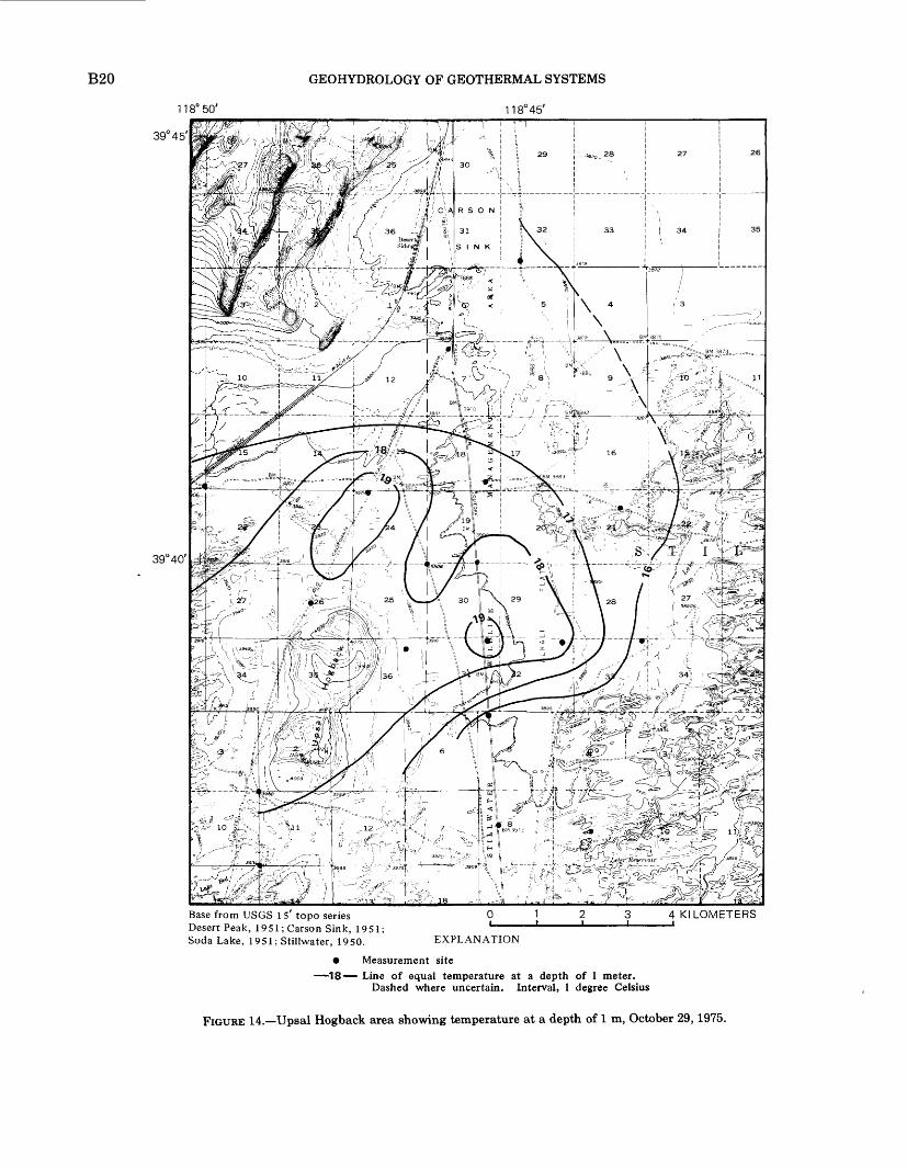
TEMPERATURE SURVEY ON OCTOBER 29, 1975
By late October 1975, 20 test wells and 18 1-m temperature holes had been completed. Sites of some of the test wells were selected on the basis of the 1-m survey in June. However, the pattern of the anomaly indicated by the 1-m survey on October 29,1975 was appreciably different from that indicated by the survey on June 15. Instead of an increase in temperature toward Upsal Hogback, two thermal maxima appeared in the October survey. The first maximum was centered at the test well mentioned above, and a second, somewhat broader, maximum was centered about 2 km north of the Hogback (fig. 14).
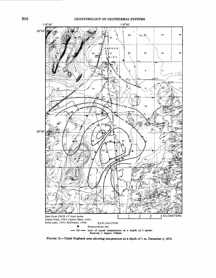
TEMPERATURE SURVEY ON DECEMBER 2, 1975
The final temperature measurements at 1-m depth near Upsal Hogback were made at 28 sites on December 2, 1975. The thermal anomaly defined by this survey was generally similar to that defined by
22110
100
90
80
70
60au. OIa. LU Q<
<ui 50CCD H < CCUJa.01H 40
30
20
22
TEMPERATURE SURVEYS IN GEOTHERMAL EXPLORATION IN NEVADA
24 26 28 30 32 34
B17
1
36
I
T20=8.43T 1 -180.7
r2=0.95
O
I
110
100
90
80
70
60
50
40
30
20
24 3626 28 30 32 34
TEMPERATURE AT A DEPTH OF 1 m (T.,), IN DEGREES CELSIUS
FIGURE 11.—Correlation of temperatures at a depth of 20 m with temperatures at a depth of 1 m in Soda Lakes area, September 1974.
B18 GEOHYDROLOGY OF GEOTHERMAL SYSTEMS118° 45'
39 40
Base from USGS 15' topo series Desert Peak, 1951; Carson Sink, 1951; Soda Lake, 1951; Stillwater, 1950.
.1.0
4 KILOMETERS
EXPLANATION Test well and depth of water table, in meters
1185 —— Water-level contourAltitude of water table, in meters above mean sea level. Arrows show inferred direction of ground-water flow
FIGURE 12.—Upsal Hogback area showing depth to the water table in test wells, configuration of the water table, and direction of shallow ground-water movement in July 1975.
TEMPERATURE SURVEYS IN GEOTHERMAL EXPLORATION IN NEVADA118° 50' 118°45'
B19
39°45'
39° 40'
Base from USGS 1S' topo seriesDesert Peak, 1951; Carson Sink, 1951; L~ Soda Lake, 1951; Stillwater, 1950. EXPLANATION
• Measurement site—— 20 ^— Line of equal temperature at a depth of 1 meter
Interval, 1 degree Celsius
FIGURE 13.—Upsal Hogback area showing temperature at a depth of 1 m, June 1975.
B20118° 50'
GEOHYDROLOGY OF GEOTHERMAL SYSTEMS
118° 45'
39° 45'
39° 40'
Base from USGS 15' topo series Desert Peak, 1951; Carson Sink, 1951; Soda Lake, 1951; Stillwater, 1950. EXPLANATION
• Measurement site—18-—• Line of equal temperature at a depth of 1 meter.
Dashed where uncertain. Interval, 1 degree Celsius
FIGURE 14.—Upsal Hogback area showing temperature at a depth of 1 m, October 29,1975.
TEMPERATURE SURVEYS IN GEOTHERMAL EXPLORATION IN NEVADA B21
the October 29 survey, but there were some differ ences in detail, owing in part to the greater number of measurement sites for the December survey (fig. 15). The center of the thermal maximum east of the Hogback was about 400 m west of where it had been in late October, and the thermal minimum between the two maxima had a greater amplitude than it did in October.
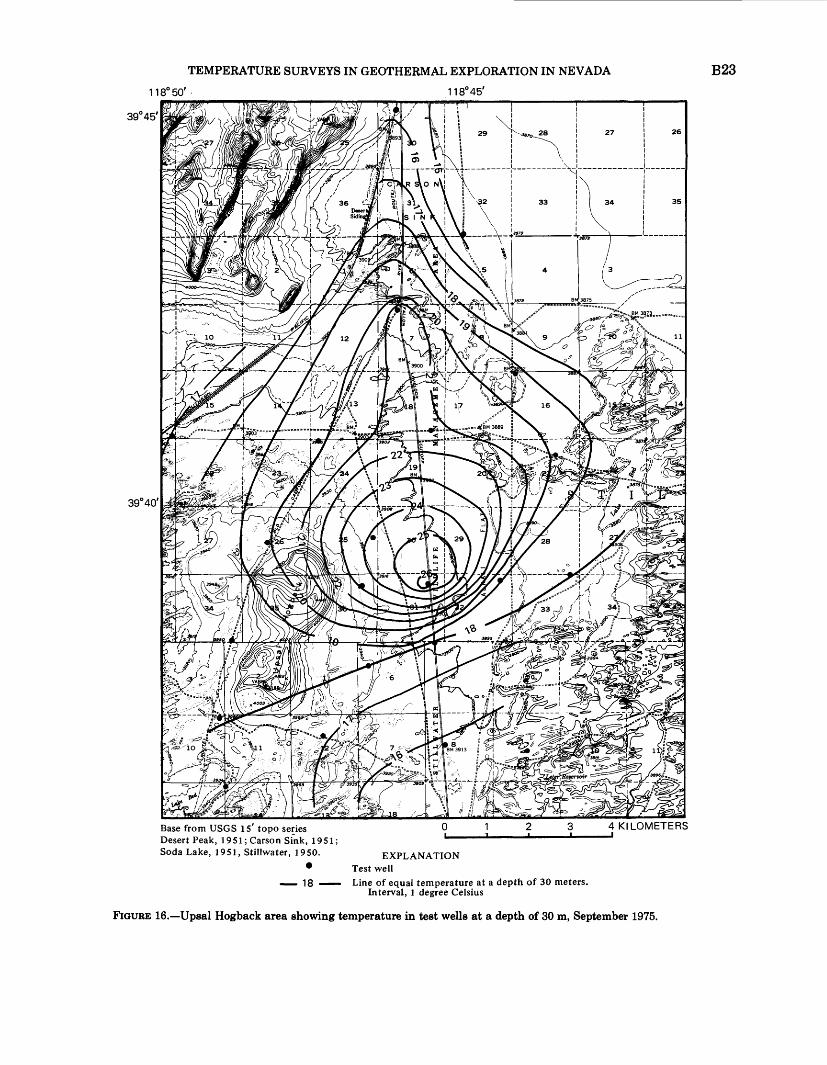
TEMPERATURE AT A DEPTH OF 30 M, SEPTEMBER 1975
By September 1975, temperatures in the 20 shallow test wells near Upsal Hogback had stabilized sufficiently so that temperatures and temperature gradients below the zone of measurable annual fluctuation could be determined with fair accuracy. As shown in figure 16, the temperature at a depth of 30 m defined a pattern that differed considerably in detail from the patterns indicated by three 1-m surveys from June to December 1975. The thermal maximum east of the Hogback, which was noted in the 1-m surveys for October and December, also was the maximum for the 30-m measurements in September. The amplitude of the anomaly at 30 m was about 12°C: temperature ranged from less than 15°C on the northeast edge to more than 26°C at the center, at the test well described earlier. The ampli tude of the equivalent anomaly at 1 m was about 3.3° -3.7°C in both the October and December surveys. In contrast to the fairly good agreement between 1-m and 30-m temperature anomalies east of the Hog back, the correlation between the patterns at the two depths appears to be rather poor in the rest of the Upsal Hogback area. The thermal maximum north of the Hogback delineated in both the October and December 1-m surveys did not appear as a separate maximum at 30 m: the minimum between the two maxima at 1 m was not present at 30 m.
CORRELATION OF TEMPERATURES AT DEPTHS OF 1 M AND 30 M
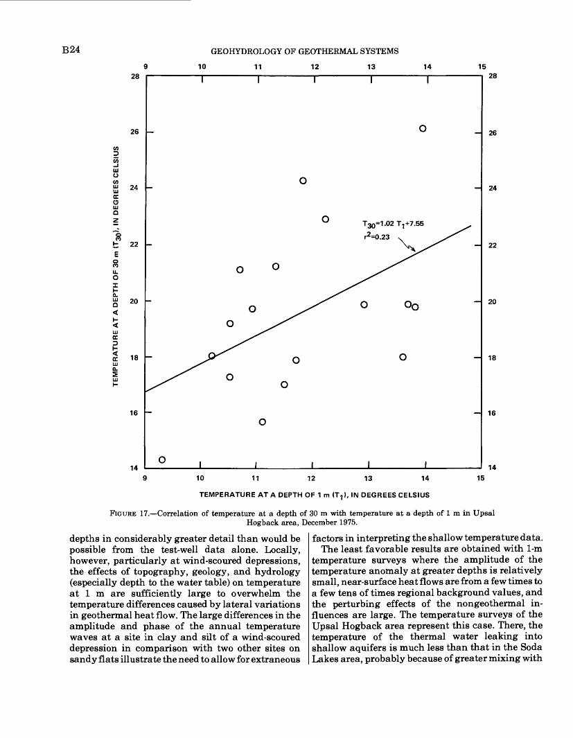
From the differences between the thermal anom alies at 30 m and 1 m described above, it might be inferred that the correlation of temperatures at the two depths also is poor. As shown in figure 17, this is indeed the case. The least-mean-squares linear regression of temperature at 30-m versus temper ature at 1-m for December 1975 is
T30 = 1.02 TI +7.55but r2 , the coefficient of determination, is only 0.23; this figure indicates a very poor correlation. Unlike the situation in the Soda Lakes area, where the amplitude of the thermal anomaly at 30 m exceeds 100°C, the amplitude of the anomaly northeast of
Upsal Hogback is only 12°C. This difference in large part accounts for the good correlation in the first area and the poor correlation in the second.
CONCLUSIONS
The results of this study confirm the general principle that the utility of temperature measure ments at a depth of 1 m in geothermal exploration is directly related to the magnitude of the temperature and heat-flow anomalies at greater depths and inversely related to the magnitude of perturbing influences such as local variations in the character and moisture content of the near-surface materials, topography, depth to the water table, vegetation, land use, and microclimate.
Temperature measurements at 1 m are most successful in delineating geothermal areas where lateral variations in temperature at greater depths are very large and where near-surface geothermal heat flows are thousands or tens of thousands times larger than background values. In the present study, the detailed survey of the small area surrounding the fumarole and abandoned steam well northeast of the Soda Lakes exemplifies the optimum case. There, the exceedingly high temperatures at 1 m, which exceed 90°C near the fumarole, almost certainly reflect heat transfer by ascending steam rather than by conduc tion. In such a situation, closely spaced temperature measurements at 1 m may be used to determine the nature and configuration of the near-surface hydrothermal-discharge system. The technique is especially applicable to the study of hot-spring areas where subsurface leakage of thermal water from the conduit system is suspected, or to areas like the one surrounding the steam well, where steam rather than thermal water is present near the surface.
Somewhat more equivocal results are obtained with 1-m temperature surveys where convective heat transport by rising steam or hot water does not extend to the land surface or where geologic, topographic, hydrologic, and other factors not related directly to geothermal heat flow are highly variable. The temperature surveys of the Soda Lakes area in November 1973 and in June and September 1974 are examples of this case. The general configuration of the thermal anomaly resulting from hydrothermal discharge into a shallow aquifer system had been established in that area on the basis of temperature surveys in test wells 20-50 m deep. Good correlation between temperature at 20 m and temperatures at 1 m at the test-well sites (fig. 11) suggested that the data for the 1-m surveys could be used with some assurance to infer the nature and configuration of the thermal anomaly at greater
B22118° 50'
GEOHYDROLOGY OF GEOTHERMAL SYSTEMS118°45'
39°45'
39°40
Base from USGS 1 s' topo series Desert Peak, 1951; Carson Sink, 19 51; ' Soda Lake, 1951; Stillwater, 1950 EXPLANATION
• Measurement site
0 4 KILOMETERS
—— 13 —— Line of equal temperature at a depth of 1 meter. Interval, 1 degree Celsius
FIGURE 15.—Upsal Hogback area showing temperature at a depth of 1 m, December 2, 1975.
TEMPERATURE SURVEYS IN GEOTHERMAL EXPLORATION IN NEVADA118°50' .118*45'
39°45'
B23
39°40'
0Base from USGS is' topo seriesDesert Peak, 1951; Carson Sink, 1951; ""—Soda Lake, 1951, Stillwater, 1950. EXPLANATION
• Test well —— 18 ——
4 KILOMETERS
Line of equal temperature at a depth of 30 meters. Interval, 1 degree Celsius
FIGURE 16.—Upsal Hogback area showing temperature in test wells at a depth of 30 m, September 1975.
B24 GEOHYDROLOGY OF GEOTHERMAL SYSTEMS
10 11 12 13 14 1528
26
24
8t 22E
20
18
16
14
T30=1.02T1 +7.55
r2=0.23 v
°0
28
26
24
22
20
18
16
1410 11 12 13 14 15
TEMPERATURE AT A DEPTH OF 1 m (T.,), IN DEGREES CELSIUS
FIGURE 17.- -Correlation of temperature at a depth of 30 m with temperature at a depth of 1 m in Upsal Hogback area, December 1975.
depths in considerably greater detail than would be possible from the test-well data alone. Locally, however, particularly at wind-scoured depressions, the effects of topography, geology, and hydrology (especially depth to the water table) on temperature at 1 m are sufficiently large to overwhelm the temperature differences caused by lateral variations in geothermal heat flow. The large differences in the amplitude and phase of the annual temperature waves at a site in clay and silt of a wind-scoured depression in comparison with two other sites on sandy flats illustrate the need to allow for extraneous
factors in interpreting the shallow temperature data. The least favorable results are obtained with 1-m
temperature surveys where the amplitude of the temperature anomaly at greater depths is relatively small, near-surface heat flows are from a few times to a few tens of times regional background values, and the perturbing effects of the nongeothermal in fluences are large. The temperature surveys of the Upsal Hogback area represent this case. There, the temperature of the thermal water leaking into shallow aquifers is much less than that in the Soda Lakes area, probably because of greater mixing with
REFERENCES CITED B25
shallow, cool ground water, and the range in depth to the water table, topographic relief, and variability of geologic materials are greater than in the Soda Lakes area. As a result, temperatures at a depth of 1 m have little or no correlation with temperatures at greater depths.
The serious risk that arises in attempts to use 1-m temperature surveys in places like the Upsal Hogback area is the identification of thermal anomalies that are actually unrelated to true geothermal anomalies at greater depth. This prob lem is highlighted by the reportedly successful use of shallow temperature surveys for a variety of purposes unrelated to geothermal investigations. Such uses include mapping of buried shallow glacial aquifers (Cartwright, 1966, 1968; Carr and Blakely, 1966; Parsons, 1970); correlation of shallow temper atures and temperature fluctuations with depth to water or depth to bedrock (Birman, 1969; Cartwright, 1974); analysis of the effects of vegetative cover on the thermal regime of soils and subsoils (Singer and Brown, 1956; Pluhowski and Kantrowitz, 1963; Kane and others, 1975); mapping of buried water-bearing joints, fissures, or caverns in bedrock (Ebaugh and others, 1974); determination of stream reaches receiving ground-water discharge (Hollyday and others, 1972); and determination of the effect of various soil-management procedures in altering the thermal regime of agricultural soils (Van Duin, 1963). All these uses have one principle in common: lateral variations in geothermal heat flow or in temperature below the depth of measurable annual temperature fluctuation are considered a perturbing influence and are treated in the analysis as "noise" in the data. Thus, to the extent that the types of studies listed above are successful, the use of shallow temperature measurements in geothermal studies would be unsuccessful, and vice versa.
REFERENCES CITEDBirman, J. H., 1969, Geothermal exploration for ground water:
Geol. Soc. America Bull., v. 80, p. 617-630.Carr, D. R., and Blakely, R. F., 1966, Temperature variation at a
depth of 30 cm in clay till and outwash sand and gravel, in Symposium on remote sensing of environment (ONR and AFCRL) 4th, 1966, Proceedings, University of Michigan, Willow Run Laboratories, Ann Arbor, Michigan, p. 203-214.
Cartwright, Keros, 1966, Thermal prospecting for shallow glacial and alluvial aquifers in Illinois [abs.]: Geol. Soc. America Abs. with Program, 1966 Annual Meeting, p. 36.
———1968, Temperature prospecting for shallow glacial and alluvial aquifers in Illinois: Illinois State Geological Survey Circ. 433, 41 p.
-1974, Tracing shallow groundwater systems by soil temperatures: Water Resources Research, v. 10, no. 4, p. 847-855.
Ebaugh, W. R., Greenfield, R. J., and Parizek, R. R., 1974, Tem perature patterns in soil above caves and fractures in bedrock [abs.]: Geol. Soc. America Abs. with Programs, Cordilleran
Section 70th Annual Meeting, v. 6, no. 3, p. 171.Hardman, George, 1965, Nevada precipitation map, adapted from
map prepared by George Hardman and others, 1936: Univer sity of Nevada, Agricultural Experimental Station Bull. 183, 57 p.
Hollyday, E. F., Scherer, L. R., and Hall, Thomas, 1972, Stream groundwater interface: Temperature gradients and ground- water discharge [abs.]: Geol. Soc. America Abs. with Pro grams, Annual Meetings, v. 4, no. 12, p. 541-542.
Kane, D. L., Luthin, J. N., and Taylor, G. S., 1975, Heat and mass transfer in cold region soils: Alaska University, College, Institute of Water Resources, Publication No. IWR-65, 50 p.
Kappelmeyer, O., 1957, The use of near-surface temperature measurements for discovering anomalies due to causes at depths: Geophysical Prospecting, v. 5, no. 3, p. 239-258.
Kintzinger, P. R., 1956, Geothermal survey of hot ground near Lordsburg, New Mexico: Science, v. 124, p. 629.
Lachenbruch, A. H., 1959, Periodic heat flow in a stratified medium with application to permafrost problems: U.S. Geo logical Survey Bull. 1083-A, 36 p.
Levering, T. S., and Goode, H. D., 1963, Measuring geothermal gradients in drill holes less than 60 feet deep, East Tintic district, Utah: U.S. Geological Survey Bull. 1172, 48 p.
Morrison, R. B., 1964, Lake Lahontan: geology of the southern Carson Desert, Nevada: U.S. Geological Survey Prof. Paper 401, 156 p.
National Oceanic and Atmospheric Administration, 1975, Clima- tological Data, Nevada, Annual Summary 1975: U.S. Depart ment of Commerce, NOAA (formerly U.S. Weather Bureau), v. 90, no. 13.
Olmsted, F. H., Glancy, P. A., Harrill, J. R., Rush, F. E., and Van Denburgh, A. S., 1975, Preliminary hydrogeologic appraisal of selected hydrothermal systems in northern and central Nevada: U.S. Geological Survey open-file report 75-56,267 p.
Parasnis, D. S., 1971, Temperature extrapolation in infinite time in geothermal measurements: Geophysical Prospecting, v. 19, p. 612-614.
Parsons, M. L., 1970, Ground-water thermal regime in a glacial complex: Water Resources Research, v. 6, no. 6, p. 1701-1720.
Pluhowski, E. J., and Kantrowitz, I. H., 1963, Influence of land- surface conditions on ground-water temperatures in south western Suffolk County, Long Island, New York, in Geo logical Survey research 1963: U.S. Geological Survey Prof. Paper 475-B, p. B186-B188.
Rush, F. E., 1972, Hydrologic reconnaissance of Big and Little Soda Lakes, Churchill County, Nevada: Nevada Department of Conservation and Water Resources, Water Resources In formation Service Report 11.
Singer, I. A., and Brown, R. M., 1956, The annual variation of sub-soil temperatures about a 600-foot diameter circle: Am. Geophys. Union Transactions, v. 37, p. 743.
U.S. Geological Survey, 1972, Aeromagnetic map of parts of the Lovelock, Reno, and Millet 1° by 2° quadrangles, Nevada: U.S. Geological Survey open-file report, scale 1:250,000.
Van Duin, R. H. A., 1963, The influence of soil management on the temperature wave near the surface: Instituut voor Cultuur Technick en Waterhuishouding, Wageningen, Tech. Bull. 29, 21 p.
Van Wijk, W. R., and Derksen, W. J., 1966, Sinusoidal temperature variation in a layered soil, ch. 6 in Van Wijk, W. R., ed., Physics of plant environment: Amsterdam, Holland, North Holland Publishing Company, p. 171-209.
Wahl, R. R., 1965, An intrepretation of gravity data from the Carson area, Nevada: Stanford University, Department of Geophysics, Student Report, Stanford University, California.
•3PO 789-090/49


