Off-Policy Evaluation via Off-Policy Classification

Alex Irpan1, Kanishka Rao1, Konstantinos Bousmalis2,Chris Harris1, Julian Ibarz1, Sergey Levine1,3

1Google Brain, Mountain View, USA2DeepMind, London, UK

3University of California Berkeley, Berkeley, USA

{alexirpan,kanishkarao,konstantinos,ckharris,julianibarz,slevine}@google.com

Abstract

In this work, we consider the problem of model selection for deep reinforcementlearning (RL) in real-world environments. Typically, the performance of deepRL algorithms is evaluated via on-policy interactions with the target environment.However, comparing models in a real-world environment for the purposes of earlystopping or hyperparameter tuning is costly and often practically infeasible. Thisleads us to examine off-policy policy evaluation (OPE) in such settings. We focuson OPE for value-based methods, which are of particular interest in deep RL,with applications like robotics, where off-policy algorithms based on Q-functionestimation can often attain better sample complexity than direct policy optimization.Existing OPE metrics either rely on a model of the environment, or the use ofimportance sampling (IS) to correct for the data being off-policy. However, forhigh-dimensional observations, such as images, models of the environment canbe difficult to fit and value-based methods can make IS hard to use or even ill-conditioned, especially when dealing with continuous action spaces. In this paper,we focus on the specific case of MDPs with continuous action spaces and sparsebinary rewards, which is representative of many important real-world applications.We propose an alternative metric that relies on neither models nor IS, by framingOPE as a positive-unlabeled (PU) classification problem with the Q-functionas the decision function. We experimentally show that this metric outperformsbaselines on a number of tasks. Most importantly, it can reliably predict the relativeperformance of different policies in a number of generalization scenarios, includingthe transfer to the real-world of policies trained in simulation for an image-basedrobotic manipulation task.

1 Introduction

Supervised learning has seen significant advances in recent years, in part due to the use of large,standardized datasets [6]. When researchers can evaluate real performance of their methods on thesame data via a standardized offline metric, the progress of the field can be rapid. Unfortunately,such metrics have been lacking in reinforcement learning (RL). Model selection and performanceevaluation in RL are typically done by estimating the average on-policy return of a method in thetarget environment. Although this is possible in most simulated environments [3, 4, 37], real-worldenvironments, like in robotics, make this difficult and expensive [36]. Off-policy evaluation (OPE)has the potential to change that: a robust off-policy metric could be used together with realistic andcomplex data to evaluate the expected performance of off-policy RL methods, which would enable

33rd Conference on Neural Information Processing Systems (NeurIPS 2019), Vancouver, Canada.

arX

iv:1

906.

0162

4v3

[cs

.LG

] 2

3 N

ov 2

019

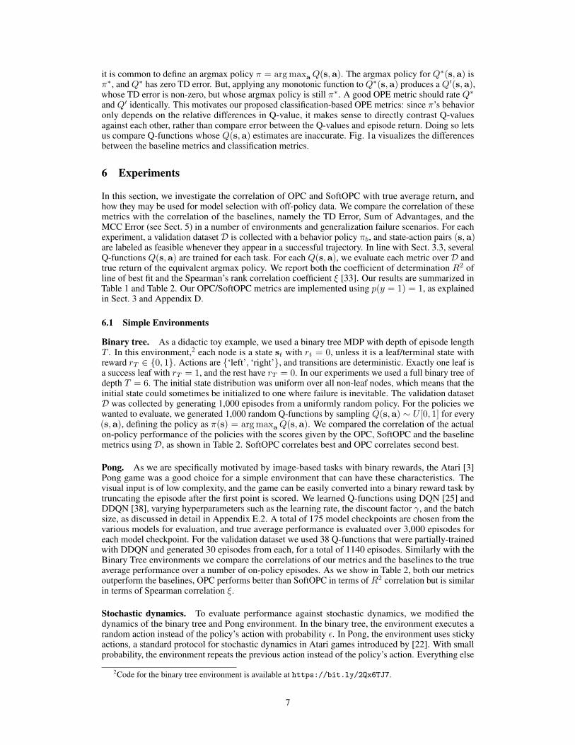
(a) Visual summary of off-policy metrics (b) Robotics grasping simulation-to-reality gap.

Figure 1: (a) Visual illustration of our method: We propose using classification-based approachesto do off-policy evaluation. Solid curves represent Q(s,a) over a positive and negative trajectory,with the dashed curve representing maxa′ Q(s,a′) along states the positive trajectory visits (thecorresponding negative curve is omitted for simplicity). Baseline approaches (blue, red) measure Q-function fit between Q(s,a) to maxa′ Q(s,a′). Our approach (purple) directly measures separationof Q(s,a) between positive and negative trajectories. (b) The visual “reality gap” of our mostchallenging task: off-policy evaluation of the generalization of image-based robotic agents trainedsolely in simulation (left) using historical data from the target real-world environment (right).

rapid progress on important real-world RL problems. Furthermore, it would greatly simplify transferlearning in RL, where OPE would enable model selection and algorithm design in simple domains(e.g., simulation) while evaluating the performance of these models and algorithms on complexdomains (e.g., using previously collected real-world data).

Previous approaches to off-policy evaluation [7, 13, 28, 35] generally use importance sampling (IS)or learned dynamics models. However, this makes them difficult to use with many modern deep RLalgorithms. First, OPE is most useful in the off-policy RL setting, where we expect to use real-worlddata as the “validation set”, but many of the most commonly used off-policy RL methods are based onvalue function estimation, produce deterministic policies [20, 38], and do not require any knowledgeof the policy that generated the real-world training data. This makes them difficult to use with IS.Furthermore, many of these methods might be used with high-dimensional observations, such asimages. Although there has been considerable progress in predicting future images [2, 19], learningsufficiently accurate models in image space for effective evaluation is still an open research problem.We therefore aim to develop an OPE method that requires neither IS nor models.

We observe that for model selection, it is sufficient to predict some statistic correlated with policyreturn, rather than directly predict policy return. We address the specific case of binary-reward MDPs:tasks where the agent receives a non-zero reward only once during an episode, at the final timestep(Sect. 2). These can be interpreted as tasks where the agent can either “succeed” or “fail” in each trial,and although they form a subset of all possible MDPs, this subset is quite representative of manyreal-world tasks, and is actively used e.g. in robotic manipulation [15, 31]. The novel contributionof our method (Sect. 3) is to frame OPE as a positive-unlabeled (PU) classification [16] problem,which provides for a way to derive OPE metrics that are both (a) fundamentally different from priormethods based on IS and model learning, and (b) perform well in practice on both simulated andreal-world tasks. Additionally, we identify and present (Sect. 4) a list of generalization scenariosin RL that we would want our metrics to be robust against. We experimentally show (Sect. 6) thatour suggested OPE metrics outperform a variety of baseline methods across all of the evaluationscenarios, including a simulation-to-reality transfer scenario for a vision-based robotic grasping task(see Fig. 1b).

2 Preliminaries

We focus on finite–horizon Markov decision processes (MDP). We define an MDP as(S,A,P,S0, r, γ). S is the state–space, A the action–space, and both can be continuous. P definestransitions to next states given the current state and action, S0 defines initial state distribution, r isthe reward function, and γ ∈ [0, 1] is the discount factor. Episodes are of finite length T : at a given

2

time-step t the agent is at state st ∈ S , samples an action at ∈ A from a policy π, receives a rewardrt = r(st,at), and observes the next state st+1 as determined by P .

The goal in RL is to learn a policy π(at|st) that maximizes the expected episode returnR(π) = Eπ[

∑Tt=0 γ

tr(st,at)]. A value of a policy for a given state st is defined as V π(st) =

Eπ[∑Tt′=t γ

t′−tr(st′ ,aπt′)] where aπt is the action π takes at state st and Eπ implies an expectation

over trajectories τ = (s1,a1, . . . , sT ,aT ) sampled from π. Given a policy π, the expected value of itsaction at at a state st is called the Q-value and is defined as Qπ(st,at) = Eπ[r(st,at) + V π(st+1)].

We assume the MDP is a binary reward MDP, which satisfies the following properties: γ = 1, thereward is rt = 0 at all intermediate steps, and the final reward rT is in {0, 1}, indicating whetherthe final state is a failure or a success. We learn Q-functions Q(s,a) and aim to evaluate policiesπ(s) = argmaxaQ(s,a).

2.1 Positive-unlabeled learning

Positive-unlabeled (PU) learning is a set of techniques for learning binary classification from partiallylabeled data, where we have many unlabeled points and some positively labeled points [16]. We willmake use of these ideas in developing our OPE metric. Positive-unlabeled data is sufficient to learn abinary classifier if the positive class prior p(y = 1) is known.

Let (X,Y ) be a labeled binary classification problem, where Y = {0, 1}. Let g : X → R be somedecision function, and let ` : R× {0, 1} → R be our loss function. Suppose we want to evaluate loss`(g(x), y) over negative examples (x, y = 0), but we only have unlabeled points x and positivelylabeled points (x, y = 1). The key insight of PU learning is that the loss over negatives can beindirectly estimated from p(y = 1). For any x ∈ X ,

p(x) = p(x|y = 1)p(y = 1) + p(x|y = 0)p(y = 0) (1)

It follows that for any f(x), EX,Y [f(x)] = p(y = 1)EX|Y=1 [f(x)] + p(y = 0)EX|Y=0 [f(x)],since by definition EX [f(x)] =

∫xp(x)f(x)dx. Letting f(x) = `(g(x), 0) and rearranging gives

p(y = 0)EX|Y=0 [`(g(x), 0)] = EX,Y [`(g(x), 0)]− p(y = 1)EX|Y=1 [`(g(x), 0)] (2)

In Sect. 3, we reduce off-policy evaluation of a policy π to a positive-unlabeled classification problem.We provide reasoning for how to estimate p(y = 1), apply PU learning to estimate classification errorwith Eqn. 2, then use the error to estimate a lower bound on return R(π) with Theorem 1.

3 Off-policy evaluation via state-action pair classification

A Q-function Q(s,a) predicts the expected return of each action a given state s. The policyπ(s) = argmaxaQ(s,a) can be viewed as a classifier that predicts the best action. We proposean off-policy evaluation method connecting off-policy evaluation to estimating validation error fora positive-unlabeled (PU) classification problem [16]. Our metric can be used with Q-functionestimation methods without requiring importance sampling, and can be readily applied in a scalableway to image-based deep RL tasks.

We present an analysis for binary reward MDPs, defined in Sec. 2. In binary reward MDPs, each(st,at) is either potentially effective, or guaranteed to lead to failure.

Definition 1. In a binary reward MDP, (st,at) is feasible if an optimal policy π∗ has non-zeroprobability of achieving success, i.e an episode return of 1, after taking at in st. A state-action pair(st,at) is catastrophic if even an optimal π∗ has zero probability of succeeding if at is taken. Astate st is feasible if there exists a feasible (st,at), and a state st is catastrophic if for all actions at,(st,at) is catastrophic.

Under this definition, the return of a trajectory τ is 1 only if all (st,at) in τ are feasible (seeAppendix A.1). This condition is necessary, but not sufficient, because success can depend on thestochastic dynamics. Since Definition 1 is defined by an optimal π∗, we can view feasible andcatastrophic as binary labels that are independent of the policy π we are evaluating. Viewing π as aclassifier, we relate the classification error of π to a lower bound for return R(π).

3

Theorem 1. Given a binary reward MDP and a policy π, let c(st,at) be the probability thatstochastic dynamics bring a feasible (st,at) to a catastrophic st+1, with c = maxs,a c(s,a). Let ρ+t,πdenote the state distribution at time t, given that π was followed, all its previous actions a1, · · · ,at−1were feasible, and st is feasible. Let A−(s) denote the set of catastrophic actions at state s, and let

εt = Eρ+t,π[∑

a∈A−(st) π(a|st)]

be the per-step expectation of π making its first mistake at time t,

with ε = 1T

∑Ti=1 εt being average error over all (st,at). Then R(π) ≥ 1− T (ε+ c).

See Appendix A.2 for the proof. For the deterministic case (c = 0), we can take inspiration fromimitation learning behavioral cloning bounds in Ross & Bagnell [32] to prove the same result. Thisalternate proof is in Appendix A.3.

A smaller error ε gives a higher lower bound on return, which implies a better π. This leavesestimating ε. The primary challenge with this approach is that we do not have negative labels – thatis, for trials that receive a return of 0 in the validation set, we do not know which (s,a) were in factcatastrophic, and which were recoverable. We discuss how we address this problem next.

3.1 Missing negative labels

Recall that (st,at) is feasible if π∗ has a chance of succeeding after action at. Since π∗ is at least asgood as πb, whenever πb succeeds, all tuples (st,at) in the trajectory τ must be feasible. However,the converse is not true, since failure could come from poor luck or suboptimal actions. Our keyinsight is that this is an instance of the positive-unlabeled (PU) learning problem from Sect. 2.1,where πb positively labels some (s,a) and the remaining are unlabeled. This lets us use ideas fromPU learning to estimate error.

In the RL setting, inputs (s,a) are from X = S × A, labels {0, 1} correspond to{catastrophic, feasible} labels, and a natural choice for the decision function g is g(s,a) =Q(s,a), since Q(s,a) should be high for feasible (s,a) and low for catastrophic (s,a). We aim toestimate ε, the probability that π takes a catastrophic action – i.e., that (s, π(s)) is a false positive.Note that if (s, π(s)) is predicted to be catastrophic, but is actually feasible, this false-negative doesnot impact future reward – since the action is feasible, there is still some chance of success. We wantjust the false-positive risk, ε = p(y = 0)EX|Y=0 [`(g(x), 0)]. This is the same as Eqn. 2, and usingg(s,a) = Q(s,a) gives

ε = E(s,a) [`(Q(s,a), 0)]− p(y = 1)E(s,a),y=1 [`(Q(s,a), 0)] . (3)

Eqn. 3 is the core of all our proposed metrics. While it might at first seem that the class prior p(y = 1)should be task-dependent, recall that the error εt is the expectation over the state distribution ρ+t,π,where the actions a1, · · · ,at−1 were all feasible. This is equivalent to following an optimal “expert”policy π∗, and although we are estimating εt from data generated by behavior policy πb, we shouldmatch the positive class prior p(y = 1) we would observe from expert π∗. Expert π∗ will alwayspick feasible actions. Therefore, although the validation dataset will likely have both successes andfailures, a prior of p(y = 1) = 1 is the ideal prior, and this holds independently of the environment.We illustrate this further with a didactic example in Sect. 6.1.

Theorem 1 relies on estimating ε over the distribution ρ+t,π, but our dataset D is generated by anunknown behavior policy πb. A natural approach here would be importance sampling (IS) [7],but: (a) we assume no knowledge of πb, and (b) IS is not well-defined for deterministic poli-cies π(s) = argmaxaQ(s,a). Another approach is to subsample D to transitions (s,a) wherea = π(s) [21]. This ensures an on-policy evaluation, but can encounter finite sample issues if πbdoes not sample π(s) frequently enough. Therefore, we assume classification error over D is a goodenough proxy that correlates well with classification error over ρ+t,π. This is admittedly a strongassumption, but empirical results in Sect. 6 show surprising robustness to distributional mismatch.This assumption is reasonable if D is broad (e.g., generated by a sufficiently random policy), but mayproduce pessimistic estimates when potential feasible actions in D are unlabeled.

3.2 Off-policy classification for OPE

Based off of the derivation from Sect. 3.1, our proposed off-policy classification (OPC) scoreis defined by the negative loss when ` in Eqn. 3 is the 0-1 loss. Let b be a threshold, with

4

`(Q(s,a), Y ) = 12 +

(12 − Y

)sign(Q(s,a)− b). This gives

OPC(Q) = p(y = 1)E(s,a),y=1

[1Q(s,a)>b

]− E(s,a)

[1Q(s,a)>b

]. (4)

To be fair to each Q(s,a), threshold b is set separately for each Q-function to maximize OPC(Q).Given N transitions and Q(s,a) for all (s,a) ∈ D, this can be done in O(N logN) time per Q-function (see Appendix B). This avoids favoring Q-functions that systematically overestimate orunderestimate the true value.

Alternatively, ` can be a soft loss function. We experimented with `(Q(s,a), Y ) = (1− 2Y )Q(s,a),which is minimized when Q(s,a) is large for Y = 1 and small for Y = 0. The negative of this lossis called the SoftOPC.

SoftOPC(Q) = p(y = 1)E(s,a),y=1 [Q(s,a)]− E(s,a) [Q(s,a)] . (5)

If episodes have different lengths, to avoid focusing on long episodes, transitions (s,a) from anepisode of length T are weighted by 1

T when estimating SoftOPC. Pseudocode is in Appendix B.

Although our derivation is for binary reward MDPs, both the OPC and SoftOPC are purely evaluationtime metrics, and can be applied to Q-functions trained with dense rewards or reward shaping, aslong as the final evaluation uses a sparse binary reward.

3.3 Evaluating OPE metrics

The standard evaluation method for OPE is to report MSE to the true episode return [21, 35]. However,our metrics do not estimate episode return directly. The OPC(Q)’s estimate of ε will differ from thetrue value, since it is estimated over our dataset D instead of over the distribution ρ+t,π. Meanwhile,SoftOPC(Q) does not estimate ε directly due to using a soft loss function. Despite this, the OPC andSoftOPC are still useful OPE metrics if they correlate well with ε or episode return R(π).

We propose an alternative evaluation method. Instead of reporting MSE, we train a large suiteof Q-functions Q(s,a) with different learning algorithms, evaluating true return of the equivalentargmax policy for each Q(s,a), then compare correlation of the metric to true return. We report twocorrelations, the coefficient of determination R2 of line of best fit, and the Spearman rank correlationξ [33].1 R2 measures confidence in how well our linear best fit will predict returns of new models,whereas ξ measures confidence that the metric ranks different policies correctly, without assuming alinear best fit.

4 Applications of OPE for transfer and generalization

Off-policy evaluation (OPE) has many applications. One is to use OPE as an early stopping ormodel selection criteria when training from off-policy data. Another is applying OPE to validationdata collected in another domain to measure generalization to new settings. Several papers [5, 27,30, 39, 40] have examined overfitting and memorization in deep RL, proposing explicit train-testenvironment splits as benchmarks for RL generalization. Often, these test environments are defined insimulation, where it is easy to evaluate the policy in the test environment. This is no longer sufficientfor real-world settings, where test environment evaluation can be expensive. In real-world problems,off-policy evaluation is an inescapable part of measuring generalization performance in an efficient,tractable way. To demonstrate this, we identify a few common generalization failure scenarios facedin reinforcement learning, applying OPE to each one. When there is insufficient off-policy trainingdata and new data is not collected online, models may memorize state-action pairs in the trainingdata. RL algorithms collect new on-policy data with high frequency. If training data is generatedin a systematically biased way, we have mismatched off-policy training data. The model fails togeneralize because systemic biases cause the model to miss parts of the target distribution. Finally,models trained in simulation usually do not generalize to the real-world, due to the training and testdomain gap: the differences in the input space (see Fig. 1b and Fig. 2) and the dynamics. All of thesescenarios are, in principle, identifiable by off-policy evaluation, as long as validation is done againstdata sampled from the final testing environment. We evaluate our proposed and baseline metricsacross all these scenarios.

1We slightly abuse notation here, and should clarify that R2 is used to symbolize the coefficient of determi-nation and should not be confused with R(π), the average return of a policy π.

5

(a) Simulated samples (b) Real samples

Figure 2: An example of a training and test domain gap. We display this with a robotic graspingtask. Left: Images used during training, from (a) simulated grasping over procedurally generatedobjects; and from (b) the real-world, with a varied collection of everyday physical objects.

5 Related work

Off-policy policy evaluation (OPE) predicts the return of a learned policy π from a fixed off-policydataset D, generated by one or more behavior policies πb. Prior works [7, 10, 13, 21, 28, 34] doso with importance sampling (IS) [11], MDP modeling, or both. Importance sampling requiresquerying π(a|s) and πb(a|s) for any s ∈ D, to correct for the shift in state-action distributions. InRL, the cumulative product of IS weights along τ is used to weight its contribution to π’s estimatedvalue [28]. Several variants have been proposed, such as step-wise IS and weighted IS [23]. InMDP modeling, a model is fitted to D, and π is rolled out in the learned model to estimate averagereturn [13, 24]. The performance of these approaches is worse if dynamics or reward are poorlyestimated, which tends to occur for image-based tasks. Improving these models is an active researchquestion [2, 19]. State of the art methods combine IS-based estimators and model-based estimatorsusing doubly robust estimation and ensembles to produce improved estimators with theoreticalguarantees [7, 8, 10, 13, 35].

These IS and model-based OPE approaches assume importance sampling or model learning arefeasible. This assumption often breaks down in modern deep RL approaches. When πb is unknown,πb(a|s) cannot be queried. When doing value-based RL with deterministic policies, π(a|s) isundefined for off-policy actions. When working with high-dimensional observations, model learningis often too difficult to learn a reliable model for evaluation.

Many recent papers [5, 27, 30, 39, 40] have defined train-test environment splits to evaluate RLgeneralization, but define test environments in simulation where there is no need for OPE. Wedemonstrate how OPE provides tools to evaluate RL generalization for real-world environments.While to our knowledge no prior work has proposed a classification-based OPE approach, severalprior works have used supervised classifiers to predict transfer performance from a few runs in thetest environment [17, 18]. To our knowledge, no other OPE papers have shown results for largeimage-based tasks where neither importance sampling nor model learning are viable options.

Baseline metrics Since we assume importance-sampling and model learning are infeasible, manycommon OPE baselines do not fit our problem setting. In their place, we use other Q-learning basedmetrics that also do not need importance sampling or model learning and only require a Q(s,a)estimate. The temporal-difference error (TD Error) is the standard Q-learning training loss, andFarahmand & Szepesvári [9] proposed a model selection algorithm based on minimizing TD error.The discounted sum of advantages (

∑t γ

tAπ) relates the difference in values V πb(s)− V π(s) to thesum of advantages

∑t γ

tAπ(s,a) over data from πb, and was proposed by Kakade & Langford [14]and Murphy [26]. Finally, the Monte Carlo corrected error (MCC Error) is derived by arranging thediscounted sum of advantages into a squared error, and was used as a training objective by Quillenet al. [29]. The exact expression of each of these metrics is in Appendix C.

Each of these baselines represents a different way to measure how well Q(s,a) fits the true return.However, it is possible to learn a good policy π even when Q(s,a) fits the data poorly. In Q-learning,

6

it is common to define an argmax policy π = argmaxaQ(s,a). The argmax policy for Q∗(s,a) isπ∗, and Q∗ has zero TD error. But, applying any monotonic function to Q∗(s,a) produces a Q′(s,a),whose TD error is non-zero, but whose argmax policy is still π∗. A good OPE metric should rate Q∗and Q′ identically. This motivates our proposed classification-based OPE metrics: since π’s behavioronly depends on the relative differences in Q-value, it makes sense to directly contrast Q-valuesagainst each other, rather than compare error between the Q-values and episode return. Doing so letsus compare Q-functions whose Q(s,a) estimates are inaccurate. Fig. 1a visualizes the differencesbetween the baseline metrics and classification metrics.

6 Experiments

In this section, we investigate the correlation of OPC and SoftOPC with true average return, andhow they may be used for model selection with off-policy data. We compare the correlation of thesemetrics with the correlation of the baselines, namely the TD Error, Sum of Advantages, and theMCC Error (see Sect. 5) in a number of environments and generalization failure scenarios. For eachexperiment, a validation dataset D is collected with a behavior policy πb, and state-action pairs (s,a)are labeled as feasible whenever they appear in a successful trajectory. In line with Sect. 3.3, severalQ-functions Q(s,a) are trained for each task. For each Q(s,a), we evaluate each metric over D andtrue return of the equivalent argmax policy. We report both the coefficient of determination R2 ofline of best fit and the Spearman’s rank correlation coefficient ξ [33]. Our results are summarized inTable 1 and Table 2. Our OPC/SoftOPC metrics are implemented using p(y = 1) = 1, as explainedin Sect. 3 and Appendix D.

6.1 Simple Environments

Binary tree. As a didactic toy example, we used a binary tree MDP with depth of episode lengthT . In this environment,2 each node is a state st with rt = 0, unless it is a leaf/terminal state withreward rT ∈ {0, 1}. Actions are {‘left’, ‘right’}, and transitions are deterministic. Exactly one leaf isa success leaf with rT = 1, and the rest have rT = 0. In our experiments we used a full binary tree ofdepth T = 6. The initial state distribution was uniform over all non-leaf nodes, which means that theinitial state could sometimes be initialized to one where failure is inevitable. The validation datasetD was collected by generating 1,000 episodes from a uniformly random policy. For the policies wewanted to evaluate, we generated 1,000 random Q-functions by sampling Q(s,a) ∼ U [0, 1] for every(s,a), defining the policy as π(s) = argmaxaQ(s,a). We compared the correlation of the actualon-policy performance of the policies with the scores given by the OPC, SoftOPC and the baselinemetrics using D, as shown in Table 2. SoftOPC correlates best and OPC correlates second best.

Pong. As we are specifically motivated by image-based tasks with binary rewards, the Atari [3]Pong game was a good choice for a simple environment that can have these characteristics. Thevisual input is of low complexity, and the game can be easily converted into a binary reward task bytruncating the episode after the first point is scored. We learned Q-functions using DQN [25] andDDQN [38], varying hyperparameters such as the learning rate, the discount factor γ, and the batchsize, as discussed in detail in Appendix E.2. A total of 175 model checkpoints are chosen from thevarious models for evaluation, and true average performance is evaluated over 3,000 episodes foreach model checkpoint. For the validation dataset we used 38 Q-functions that were partially-trainedwith DDQN and generated 30 episodes from each, for a total of 1140 episodes. Similarly with theBinary Tree environments we compare the correlations of our metrics and the baselines to the trueaverage performance over a number of on-policy episodes. As we show in Table 2, both our metricsoutperform the baselines, OPC performs better than SoftOPC in terms of R2 correlation but is similarin terms of Spearman correlation ξ.

Stochastic dynamics. To evaluate performance against stochastic dynamics, we modified thedynamics of the binary tree and Pong environment. In the binary tree, the environment executes arandom action instead of the policy’s action with probability ε. In Pong, the environment uses stickyactions, a standard protocol for stochastic dynamics in Atari games introduced by [22]. With smallprobability, the environment repeats the previous action instead of the policy’s action. Everything else

2Code for the binary tree environment is available at https://bit.ly/2Qx6TJ7.

7

is unchanged. Results in Table 1. In more stochastic environments, all metrics drop in performancesince Q(s, a) has less control over return, but OPC and SoftOPC consistently correlate better thanthe baselines.

Table 1: Results from stochastic dynamics experiments. For each metric (leftmost column), we reportR2 of line of best fit and Spearman rank correlation coefficient ξ for each environment (top row), overstochastic versions of the binary tree and Pong tasks from Sect. 6.1. Correlation drops as stochasticityincreases, but our proposed metrics (last two rows) consistently outperform baselines.

Stochastic Tree 1-Success Leaf Pong Sticky Actionsε = 0.4 ε = 0.6 ε = 0.8 Sticky 10% Sticky 25%R2 ξ R2 ξ R2 ξ R2 ξ R2 ξ

TD Err 0.01 -0.07 0.00 -0.05 0.00 -0.05 0.05 -0.16 0.07 -0.15∑γtAπ 0.00 0.01 0.01 -0.07 0.00 -0.02 0.04 -0.29 0.01 -0.22

MCC Err 0.07 -0.27 0.01 -0.06 0.01 -0.11 0.02 -0.32 0.00 -0.18OPC (Ours) 0.13 0.38 0.01 0.08 0.03 0.19 0.48 0.73 0.33 0.66SoftOPC (Ours) 0.14 0.39 0.03 0.18 0.04 0.20 0.33 0.67 0.16 0.58

6.2 Vision-based Robotic Grasping

Our main experimental results were on simulated and real versions of a robotic environment and avision-based grasping task, following the setup from Kalashnikov et al. [15], the details of whichwe briefly summarize. The observation at each time-step is a 472× 472 RGB image from a cameraplaced over the shoulder of a robotic arm, of the robot and a bin of objects, as shown in Fig. 1b. At thestart of an episode, objects are randomly dropped in a bin in front of the robot. The goal is to graspany of the objects in that bin. Actions include continuous Cartesian displacements of the gripper, andthe rotation of the gripper around the z-axis. The action space also includes three discrete commands:“open gripper”, “close gripper”, and “terminate episode”. Rewards are sparse, with r(sT ,aT ) = 1if any object is grasped and 0 otherwise. All models are trained with the fully off-policy QT-Optalgorithm as described in Kalashnikov et al. [15].

In simulation we define a training and a test environment by generating two distinct sets of 5 objectsthat are used for each, shown in Fig. 8. In order to capture the different possible generalization failurescenarios discussed in Sect. 4, we trained Q-functions in a fully off-policy fashion with data collectedby a hand-crafted policy with a 60% grasp success rate and ε-greedy exploration (with ε=0.1) withtwo different datasets both from the training environment. The first consists of 100, 000 episodes,with which we can show we have insufficient off-policy training data to perform well even in thetraining environment. The second consists of 900, 000 episodes, with which we can show we havesufficient data to perform well in the training environment, but due to mismatched off-policy trainingdata we can show that the policies do not generalize to the test environment (see Fig. 8 for objectsand Appendix E.3 for the analysis). We saved policies at different stages of training which resulted in452 policies for the former case and 391 for the latter. We evaluated the true return of these policieson 700 episodes on each environment and calculated the correlation with the scores assigned by theOPE metrics based on held-out validation sets of 50, 000 episodes from the training environment and10, 000 episodes from the test one, which we show in Table 2.

Table 2: Summarized results of Experiments section. For each metric (leftmost column), we reportR2

of line of best fit and Spearman rank correlation coefficient ξ for each environment (top row). Theseare: the binary tree and Pong tasks from Sect. 6.1, simulated grasping with train or test objects, andreal-world grasping from Sect. 6.2. Baseline metrics are discussed in Sect. 5, and our metrics (OPC,SoftOPC) are discussed in Sect. 3. Occasionally, some baselines correlate well, but our proposedmetrics (last two rows) are consistently among the best metrics for each environment.

Tree (1 Succ) Pong Sim Train Sim Test Real-WorldR2 ξ R2 ξ R2 ξ R2 ξ R2 ξ

TD Err 0.02 -0.15 0.05 -0.18 0.02 -0.37 0.10 -0.51 0.17 0.48∑γtAπ 0.00 0.00 0.09 -0.32 0.74 0.81 0.74 0.78 0.12 0.50

MCC Err 0.06 -0.26 0.04 -0.36 0.00 0.33 0.06 -0.44 0.01 -0.15OPC (Ours) 0.21 0.50 0.50 0.72 0.49 0.86 0.35 0.66 0.81 0.87SoftOPC (Ours) 0.19 0.51 0.36 0.75 0.55 0.76 0.48 0.77 0.91 0.94

The real-world version of the environment has objects that were never seen during training (seeFig. 1b and 9). We evaluated 15 different models, trained to have varying degrees of robustness to

8

the training and test domain gap, based on domain randomization and randomized–to-canonicaladaptation networks [12].3 Out of these, 7 were trained on-policy purely in simulation. True averagereturn was evaluated over 714 episodes with 7 different sets of objects, and true policy real-worldperformance ranged from 17% to 91%. The validation dataset consisted of 4, 000 real-world episodes,40% of which were successful grasps and the objects used for it were separate from the ones used forfinal evaluation used for the results in Table 2.

(a) SoftOPC and return in sim (b) Scatterplot for real-world grasping

Figure 3: (a): SoftOPC in simulated grasping. Overlay of SoftOPC (red) and return (blue) insimulation for model trained with 100k grasps. SoftOPC tracks episode return. (b): Scatterplots forOPE metrics and real-world grasp success. Scatterplots for

∑γt′Aπ(st′ ,at′) (left) and SoftOPC

(right) for the Real-World grasping task. Each point is a different grasping model. Shaded regionsare a 95% confidence interval.

∑γt′Aπ(st′ ,at′) works in simulation but fails on real data, whereas

SoftOPC works well in both.

6.3 Discussion

Table 2 shows R2 and ξ for each metric for the different environments we considered. Our proposedSoftOPC and OPC consistently outperformed the baselines, with the exception of the simulatedrobotic test environment, on which the SoftOPC performed almost as well as the discounted sumof advantages on the Spearman correlation (but worse on R2). However, we show that SoftOPCmore reliably ranks policies than the baselines for real-world performance without any real-worldinteraction, as one can also see in Fig. 3b. The same figure shows the sum of advantages metric thatworks well in simulation performs poorly in the real-world setting we care about. Appendix F includesadditional experiments showing correlation mostly unchanged on different validation datasets.

Furthermore, we demonstrate that SoftOPC can track the performance of a policy acting in thesimulated grasping environment, as it is training in Fig. 3a, which could potentially be useful forearly stopping. Finally, SoftOPC seems to be performing slightly better than OPC in most of theexperiments. We believe this occurs because the Q-functions compared in each experiment tend tohave similar magnitudes. Preliminary results in Appendix H suggest that when Q-functions havedifferent magnitudes, OPC might outperform SoftOPC.

7 Conclusion and future work

We proposed OPC and SoftOPC, classification-based off-policy evaluation metrics that can be usedtogether with Q-learning algorithms. Our metrics can be used with binary reward tasks: tasks whereeach episode results in either a failure (zero return) or success (a return of one). While this classof tasks is a substantial restriction, many practical tasks actually fall into this category, includingthe real-world robotics tasks in our experiments. The analysis of these metrics shows that it canapproximate the expected return in deterministic binary reward MDPs. Empirically, we find that OPCand the SoftOPC variant correlate well with performance across several environments, and predictgeneralization performance across several scenarios. including the simulation-to-reality scenario, acritical setting for robotics. Effective off-policy evaluation is critical for real-world reinforcementlearning, where it provides an alternative to expensive real-world evaluations during algorithmdevelopment. Promising directions for future work include developing a variant of our method that isnot restricted to binary reward tasks. We include some initial work in Appendix J. However, even inthe binary setting, we believe that methods such as ours can provide for a substantially more practicalpipeline for evaluating transfer learning and off-policy reinforcement learning algorithms.

3For full details of each of the models please see Appendix E.4.

9

Acknowledgements

We would like to thank Razvan Pascanu, Dale Schuurmans, George Tucker, and Paul Wohlhart forvaluable discussions.

References[1] Arjona-Medina, J. A., Gillhofer, M., Widrich, M., Unterthiner, T., Brandstetter, J., and Hochre-

iter, S. Rudder: Return decomposition for delayed rewards. arXiv preprint arXiv:1806.07857,2018.

[2] Babaeizadeh, M., Finn, C., Erhan, D., Campbell, R. H., and Levine, S. Stochastic variationalvideo prediction. In International Conference on Representation Learning, 2018.

[3] Bellemare, M. G., Naddaf, Y., Veness, J., and Bowling, M. The arcade learning environment:An evaluation platform for general agents. Journal of Artificial Intelligence Research, 47:253–279, 2013.

[4] Brockman, G., Cheung, V., Pettersson, L., Schneider, J., Schulman, J., Tang, J., and Zaremba,W. Openai gym. arXiv preprint arXiv:1606.01540, 2016.

[5] Cobbe, K., Klimov, O., Hesse, C., Kim, T., and Schulman, J. Quantifying generalization inreinforcement learning. arXiv preprint arXiv:1812.02341, 2018.

[6] Deng, J., Dong, W., Socher, R., Li, L.-J., Li, K., and Fei-Fei, L. ImageNet: A Large-ScaleHierarchical Image Database. In CVPR, 2009, 2009.

[7] Dudik, M., Langford, J., and Li, L. Doubly robust policy evaluation and learning. In ICML,March 2011.

[8] Dudík, M., Erhan, D., Langford, J., Li, L., et al. Doubly robust policy evaluation and optimiza-tion. Statistical Science, 29(4):485–511, 2014.

[9] Farahmand, A.-M. and Szepesvári, C. Model selection in reinforcement learning. Mach. Learn.,85(3):299–332, December 2011.

[10] Hanna, J. P., Stone, P., and Niekum, S. Bootstrapping with models: Confidence intervals forOff-Policy evaluation. In Proceedings of the 16th Conference on Autonomous Agents andMultiAgent Systems, AAMAS ’17, pp. 538–546, Richland, SC, 2017. International Foundationfor Autonomous Agents and Multiagent Systems.

[11] Horvitz, D. G. and Thompson, D. J. A generalization of sampling without replacement from afinite universe. Journal of the American statistical Association, 47(260):663–685, 1952.

[12] James, S., Wohlhart, P., Kalakrishnan, M., Kalashnikov, D., Irpan, A., Ibarz, J., Levine, S.,Hadsell, R., and Bousmalis, K. Sim-to-real via sim-to-sim: Data-efficient robotic grasping viarandomized-to-canonical adaptation networks. In IEEE Conference on Computer Vision andPattern Recognition, March 2019.

[13] Jiang, N. and Li, L. Doubly robust off-policy value evaluation for reinforcement learning.November 2015.

[14] Kakade, S. and Langford, J. Approximately optimal approximate reinforcement learning. InICML, 2002.

[15] Kalashnikov, D., Irpan, A., Pastor, P., Ibarz, J., Herzog, A., Jang, E., Quillen, D., Holly, E.,Kalakrishnan, M., Vanhoucke, V., et al. Qt-opt: Scalable deep reinforcement learning forvision-based robotic manipulation. arXiv preprint arXiv:1806.10293, 2018.

[16] Kiryo, R., Niu, G., du Plessis, M. C., and Sugiyama, M. Positive-unlabeled learning withnon-negative risk estimator. In NeurIPS, pp. 1675–1685, 2017.

[17] Koos, S., Mouret, J.-B., and Doncieux, S. Crossing the reality gap in evolutionary robotics bypromoting transferable controllers. In Proceedings of the 12th annual conference on Geneticand evolutionary computation, pp. 119–126. ACM, 2010.

10

[18] Koos, S., Mouret, J.-B., and Doncieux, S. The transferability approach: Crossing the realitygap in evolutionary robotics. IEEE Transactions on Evolutionary Computation, 17(1):122–145,2012.

[19] Lee, A. X., Zhang, R., Ebert, F., Abbeel, P., Finn, C., and Levine, S. Stochastic adversarialvideo prediction. arXiv preprint arXiv:1804.01523, 2018.

[20] Lillicrap, T. P., Hunt, J. J., Pritzel, A., Heess, N., Erez, T., Tassa, Y., Silver, D., and Wierstra, D.Continuous control with deep reinforcement learning. arXiv preprint arXiv:1509.02971, 2015.

[21] Liu, Y., Gottesman, O., Raghu, A., Komorowski, M., Faisal, A., Doshi-Velez, F., and Brunskill,E. Representation balancing mdps for off-policy policy evaluation. In NeurIPS, 2018.

[22] Machado, M. C., Bellemare, M. G., Talvitie, E., Veness, J., Hausknecht, M., and Bowling, M.Revisiting the arcade learning environment: Evaluation protocols and open problems for generalagents. Journal of Artificial Intelligence Research, 61:523–562, 2018.

[23] Mahmood, A. R., van Hasselt, H. P., and Sutton, R. S. Weighted importance sampling foroff-policy learning with linear function approximation. In Advances in Neural InformationProcessing Systems, pp. 3014–3022, 2014.

[24] Mannor, S., Simester, D., Sun, P., and Tsitsiklis, J. N. Bias and variance approximation in valuefunction estimates. Management Science, 53(2):308–322, 2007.

[25] Mnih, V., Kavukcuoglu, K., Silver, D., Rusu, A. A., Veness, J., Bellemare, M. G., Graves,A., Riedmiller, M., Fidjeland, A. K., Ostrovski, G., et al. Human-level control through deepreinforcement learning. Nature, 518(7540):529, 2015.

[26] Murphy, S. A. A generalization error for Q-Learning. J. Mach. Learn. Res., 6:1073–1097, July2005.

[27] Nichol, A., Pfau, V., Hesse, C., Klimov, O., and Schulman, J. Gotta learn fast: A new benchmarkfor generalization in rl. arXiv preprint arXiv:1804.03720, 2018.

[28] Precup, D., Sutton, R. S., and Singh, S. Eligibility traces for off-policy policy evaluation.In Proceedings of the Seventeenth International Conference on Machine Learning, 2000, pp.759–766. Morgan Kaufmann, 2000.

[29] Quillen, D., Jang, E., Nachum, O., Finn, C., Ibarz, J., and Levine, S. Deep reinforcementlearning for Vision-Based robotic grasping: A simulated comparative evaluation of Off-Policymethods. February 2018.

[30] Raghu, M., Irpan, A., Andreas, J., Kleinberg, R., Le, Q., and Kleinberg, J. Can deep reinforce-ment learning solve erdos-selfridge-spencer games? In International Conference on MachineLearning, pp. 4235–4243, 2018.

[31] Riedmiller, M., Hafner, R., Lampe, T., Neunert, M., Degrave, J., Van de Wiele, T., Mnih, V.,Heess, N., and Springenberg, J. T. Learning by playing-solving sparse reward tasks from scratch.In International Conference on Machine Learning, 2018.

[32] Ross, S. and Bagnell, D. Efficient reductions for imitation learning. In AISTATS, pp. 661–668,2010.

[33] S. Spearman, C. The proof and measurement of association between two things. The AmericanJournal of Psychology, 15:72–101, 01 1904. doi: 10.2307/1412159.

[34] Theocharous, G., Thomas, P. S., and Ghavamzadeh, M. Personalized ad recommendationsystems for life-time value optimization with guarantees. In IJCAI, pp. 1806–1812, 2015.

[35] Thomas, P. and Brunskill, E. Data-Efficient Off-Policy policy evaluation for reinforcementlearning. In International Conference on Machine Learning, pp. 2139–2148, June 2016.

[36] Thomas, P. S., Theocharous, G., and Ghavamzadeh, M. High-Confidence Off-Policy evaluation.AAAI, 2015.

11

[37] Todorov, E., Erez, T., and Tassa, Y. Mujoco: A physics engine for model-based control.In Intelligent Robots and Systems (IROS), 2012 IEEE/RSJ International Conference on, pp.5026–5033. IEEE, 2012.

[38] van Hasselt, H., Guez, A., and Silver, D. Deep reinforcement learning with double q-learning.In Thirtieth AAAI Conference on Artificial Intelligence, 2016.

[39] Zhang, A., Ballas, N., and Pineau, J. A dissection of overfitting and generalization in continuousreinforcement learning. June 2018.

[40] Zhang, C., Vinyals, O., Munos, R., and Bengio, S. A study on overfitting in deep reinforcementlearning. April 2018.

12

Appendix for Off-Policy Evaluation via Off-Policy Classification

A Classification error bound

A.1 Trajectory τ return 1⇒ all at feasible

Suppose this were not true. Then, there exists a time t where at is catastrophic. After executing saidat, it should be impossible for τ to end in a success state. However, we know τ ends in success. Bycontradiction, all (st,at) should be feasible.

A.2 Proof of Theorem 1

To bound R(π), it is easier to bound the failure rate 1 − R(π). Policy π succeeds if and only if atevery st, it selects a feasible at a feasible at, and dynamics do not take it to a catastrophic st+1. Thefailure rate is the total probability π makes its first mistake or is first brought to a catastrophic st+1,summed over all t.

The distribution ρ+t,π is defined such that ρ+t,π is the marginal state distribution at time t, conditionedon a1, · · · ,at−1 being feasible and st being feasible. This makes εt the expected probability πchoosing a catastrophic at at time t, given no mistakes earlier in the trajectory. Conditioned on this,the failure rate at time t is upper-bounded by εt + c.

1−R(π) ≤T∑t=1

p(π at feasible st) · (εt + c) (6)

≤T∑t=1

(εt + c) (7)

≤ T (ε+ c) (8)

This gives R(π) ≥ 1 − T (ε + c) as desired. This bound is tight when π is always at a feasible st,which occurs when c = 0, ε1 = ε2 = · · · = εT−1 = 0, and εT = Tε. When c > 0, this bound maybe improvable.

A.3 Alternate proof connecting to behavioral cloning in deterministic case

In a deterministic environment, we have c(s,a) = 0 for all (s,a), and a policy that only picks feasibleactions will always achieve the optimal return of 1. Any such policy can be considered an expertpolicy π∗. Since ε is defined as the 0-1 loss over states conditioned on not selecting a catastrophicaction, we can view ε as the 0-1 behavior cloning loss to an expert policy π∗. In this section, wepresent an alternate proof based on behavioral cloning bounds from Ross & Bagnell [32].

Theorem 2.1 of Ross & Bagnell [32] proves a O(T 2ε) cost bound for general MDPs. This differsfrom the O(Tε) cost derived above. The difference in bound comes because Ross & Bagnell [32]derive their proof in a general MDP, whose cost is upper bounded by 1 at every timestep. If π deviatesfrom the expert, it receives cost 1 several times, once for every future timestep. In binary rewardMDPs, we only receive this cost once, at the final timestep. Transforming the proof to incorporateour binary reward MDP assumptions lets us recover the O(Tε) upper bound from Appendix A.2. Webriefly explain the updated proof, using notation from [32] to make the connection more explicit.

Define εt as the expected 0-1 loss at time t for π under the state distribution of π∗. Since ρ+t,πcorresponds to states π visits conditioned on never picking a catastrophic action, this is the same asour definition of εt. The MDP is defined by cost instead of reward: cost C(s) of state s is 0 for alltimesteps except the final one, whereC(s) ∈ {0, 1}. Let pt be the probability π hasn’t made a mistake(w.r.t π∗) in the first t steps, dt be the state distribution conditioned on no mistakes in the first t− 1steps, and d′t be the state distribution conditioned on π making at least 1 mistake. In a general MDPwith 0 ≤ C(s) ≤ 1, total cost J(π) is bounded by J(π) ≤

∑Tt=1[pt−1Edt [Cπ(s)] + (1− pt−1)],

where the 1st term is cost while following the expert and the 2nd term is an upper bound of cost 1 if

13

outside of the expert distribution. In a binary reward MDP, since C(s) = 0 for all t except t = T , wecan ignore every term in the summation except the final one, giving

J(π) = pT−1EdT [Cπ(sT )] + (1− pT−1) (9)

Note EdT [Cπ(sT )] = εT , and as shown in the original proof, pt ≥ 1 −∑ti=1 εi. Since pT−1 is

a probability, we have pT−1EdT [Cπ(sT )] ≤ EdT [Cπ(sT )], which recovers the O(Tε) bound, andagain this is tight when ε1 = · · · = εT−1 = 0, εT = Tε.

J(π) ≤ EdT [Cπ(sT )] +

T−1∑t=1

εt =

T∑t=1

εT = Tε (10)

B Algorithm pseudocode

We first present pseudocode for SoftOPC.

SoftOPC(Q) = p(y = 1)E(s,a),y=1 [Q(s,a)]− E(s,a) [Q(s,a)] . (11)

Algorithm 1 Soft Off-Policy Classification (SoftOPC)

Require: Dataset D of trajectories τ = (s1,a1, . . . , sT ,aT ), learned Q-function Q(s,a), priorp(y = 1) (set to 1 for all experiments).

1: PositiveAverages← EMPTY _LIST2: AllAverages← EMPTY _LIST3: for (s1,a1, . . . , sT ,aT , rT ) ∈ D do4: Compute Q-values Q(s1,a1), . . . , Q(sT ,aT ).5: AverageQ← 1

T

∑tQ(st,at)

6: AllAverages.append(AverageQ)7: if rT = 1 then8: PositiveAverages.append(AverageQ)9: end if

10: end for11: return p(y = 1)AV ERAGE(PositiveAverages)−AV ERAGE(AllAverages)

Next, we present pseudocode for OPC.

OPC(Q) = p(y = 1)E(s,a),y=1

[1Q(s,a)>b

]− E(s,a)

[1Q(s,a)>b

](12)

Suppose we have N transitions, of which N+ of them have positive labels. Imagine placing eachQ(s,a) on the number line. Each Q(s,a) is annotated with a score, −1/N for unlabeled transitionsand p(y = 1)/N+ − 1/N for positive labeled transitions. Imagine sliding a line from b = −∞ tob = ∞. At b = −∞, the OPC score is p(y = 1) − 1. The OPC score only updates when this linepasses some Q(s,a) in our dataset, and is updated based on the score annotated at Q(s,a). Aftersorting by Q-value, we can find all possible OPC scores in O(N) time by moving b from −∞ to∞, noting the updated score after each Q(s,a) we pass. Given D, we sort the N transitions inO(N logN), annotate them appropriately, then compute the maximum over all OPC scores. Whendoing so, we must be careful to detect when the same Q(s,a) value appears multiple times, whichcan occur when (s,a) appears in multiple trajectories.

C Baseline metrics

We elaborate on the exact expressions used for the baseline metrics. In all baselines, aπt is theon-policy action argmaxaQ

π(st,a).

Temporal-difference error The TD error is the squared error between Q(s,a) and the 1-stepreturn estimate of the action’s value.

Est,at∼πb

[(Qπ(st,at)− (rt + γQπ(st+1,a

πt )))

2]

(13)

14

Algorithm 2 Off-Policy Classification (OPC)

Require: Dataset D of trajectories τ = (s1,a1, . . . , sT ,aT ), learned Q-function Q(s,a), priorp(y = 1) (set to 1 for all experiments).

1: N+ ← number of (s,a) ∈ D from trajectories where rT = 12: N ← number of (s,a) ∈ D3: Q-values← EMPTY _DICTIONARY4: for (s1,a1, . . . , sT ,aT , rT ) ∈ D do . Prepare annotated number line5: Compute Q-values Q(s1,a1), . . . , Q(sT ,aT ).6: for t = 1, 2, . . . , T do7: if Q(s,a) 6∈ Q-values.keys() then8: Q-values[Q(s,a)] = 09: end if

10: if rT = 1 then11: Q-values[Q(s,a)] += p(y = 1)/N+

12: else13: Q-values[Q(s,a)] += −1/N14: end if15: end for16: end for17: RunningTotal← p(y = 1)− 1 . OPC when b = −∞18: BestOPC← RunningTotal19: for b ∈Sorted(Q-values.keys()) do20: RunningTotal += Q-values[b]21: BestOPC← max(BestOPC, RunningTotal)22: end for23: return BestOPC

Discounted sum of advantages The difference of the value functions of two policies π and πb atstate st is given by the discounted sum of advantages [14, 26] of π on episodes induced by πb:

V πb(st)− V π(st) = Est,at∼πb

[T∑t′=t

γt′−tAπ(st′ ,at′)

], (14)

where γ is the discount factor and Aπ the advantage function for policy π, defined as Aπ(st,at) =Qπ(st,at)−Qπ(st,aπt ). Since V πb is fixed, estimating (14) is sufficient to compare π1 and π2. Theπ with smaller score is better.

Est,at∼πb

[T∑t′=t

γt′−tAπ(st′ ,at′)

]. (15)

Monte-Carlo estimate corrected with the discounted sum of advantages Estimating V πb(st) =Eπb [

∑t′ γ

t′−trt′ ] with the Monte-Carlo return, substituting into Eqn. (14), and rearranging gives

V π(st) = Est,at∼πb

[T∑t′=t

γt′−t (rt′ −Aπ(st′ ,at′))

](16)

With V π(st) + Aπ(st,at) = Qπ(st,at), we can obtain an approximate Q̃ estimate depending onthe whole episode:

Q̃MCC(st,at, π) = Est,at∼πb

[rt +

T∑t′=t+1

γt′−t(rt′ −Aπ(st′ ,at′))

](17)

The MCC Error is the squared error to this estimate.

Est,at∼πb

[(Qπ(st,at)− Q̃MCC(st,at, π)

)2](18)

15

Note that (18) was proposed before by Quillen et al. [29] as a training loss for a Q-learning variant,but not for the purpose of off-policy evaluation.

Eqn. (13) and Eqn. (17) share the same optimal Q-function, so assuming a perfect learning algorithm,there is no difference in information between these metrics. In practice, the Q-function will not beperfect due to errors in function approximation and optimization. Eqn. (17) is designed to rely on allfuture rewards from time t, rather than just rt. We theorized that using more of the “ground truth”from D could improve the metric’s performance in imperfect learning scenarios. This did not occurin our experiments - the MCC Error performed poorly.

D Argument for choosing p(y = 1) = 1

The positive class prior p(y = 1) should intuitively depend on the environment, since some environ-ments will have many more feasible (s,a) than others. However, recall how error ε is defined. Eachεt is defined as:

εt = Eρ+t,π

∑a∈A−(st)

π(a|st)

(19)

where state distribution ρ+t,π is defined such that a1, · · · ,at−1 were all feasible. This is equivalentto following an optimal “expert” policy π∗, and although we are estimating εt from data generatedby behavior policy πb, we should match the positive class prior p(y = 1) we would observe fromexpert π∗. Assuming the task is feasible, meaining the policy has feasible actions available fromthe start, we have R(π∗) = 1. Therefore, although the validation dataset will likely have bothsuccesses and failures, a prior of p(y = 1) = 1 is the ideal prior, and this holds independently ofthe environment. As a didactic toy example, we show this holds for a binary tree domain. In thisdomain, each node is a state, actions are {left, right}, and leaf nodes are terminal with reward 0or 1. We try p(y = 1) ∈ {0, 0.05, 0.1, · · · , 0.9, 0.95, 1} in two extremes: only 1 leaf fails, or only 1leaf succeeds. No stochasticity was added. Validation data is from the uniformly random policy. Thefrequency of feasible (s,a) varies a lot between the two extremes, but in both Spearman correlation ρmonotonically increases with p(y = 1) and was best with p(y = 1) = 1. Fig. 4 shows Spearmancorrelation of OPC and SoftOPC with respect to p(y = 1), when the tree is mostly success or failures.In both settings p(y = 1) = 1 has the best correlation.

Figure 4: Spearman correlation of SoftOPC, OPC, and baselines with varying p(y = 1). Baselinesdo not depend on p(y = 1). Correlations further from 0 are better.

From an implementation perspective, p(y = 1) = 1 is also the only choice that can be applied acrossarbitrary validation datasets. Suppose πb, the policy collecting our validation set, succeeds withprobability R(πb) = p. In the practical computation of OPC presented in Algorithm 2, we have Ntransitions, and pN of them have positive labels. Each Q(s,a) is annotated with a score: −1N forunlabeled transitions and p(y=1)

pN − 1N for positive labeled transitions. The maximal OPC score will

be the sum of all annotations within the interval [b,∞), and we maximize over b.

For unlabeled transitions, the annotation is −1/N , which is negative. Suppose the annotation forpositive transitions was negative as well. This occurs when p(y = 1)/(pN) − 1/N < 0. If every

16

annotation is negative, then the optimal choice for b is b = ∞, since the empty set has total 0 andevery non-empty subset has a negative total. This gives OPC(Q) = 0, no matter what Q(s,a) we areevaluating, which makes the OPC score entirely independent of episode return.

This degenerate case is undesirable, and happens when p(y = 1)/(pN) < 1/N , or equivalentlyp(y = 1) < p. To avoid this, we should have p(y = 1) ≥ p = R(πb). If we wish to pick a sin-gle p(y = 1) that can be applied to data from arbitrary behavior policies πb, then we shouldpick p(y = 1) ≥ R(π∗). In binary reward MDPs where π∗ can always succeed, this givesp(y = 1) ≥ R(π∗) = 1, and since the prior is a probability, it should satisfy 0 ≤ p(y = 1) ≤ 1,leaving p(y = 1) = 1 as the only option.

To complete the argument, we must handle the case where we have a binary reward MDP whereR(π∗) < 1. In a binary reward MDP, the only way to have R(π∗) < 1 is if the sampled initialstate s1 is one where (s1,a) is catastrophic for all a. From these s1, and all future st reachablefrom s1, the actions π chooses do not matter - the final return will always be 0. Since εt is definedconditioned on only executing feasible actions so far, it is reasonable to assume we only wish tocompute the expectation over states where our actions can impact reward. If we computed optimalpolicy return R(π∗) over just the initial states s1 where feasible actions exist, we have R(π∗) = 1,giving 1 ≤ p(y = 1) ≤ 1 once again.

E Experiment details

E.1 Binary tree environment details

The binary tree is a full binary tree with k = 6 levels. The initial state distribution is uni-form over all non-leaf nodes. Initial state may sometimes be initialized to one where failureis inevitable. The validation dataset is collected by generating 1,000 episodes from the uni-formly random policy. For Q-functions, we generate 1,000 random Q-functions by samplingQ(s,a) ∼ U [0, 1] for every (s,a), defining the policy as π(s) = argmaxaQ(s,a). We trypriors p(y = 1) ∈ {0, 0.05, 0.1, · · · , 0.9, 0.95, 1}. Code for this environment is available athttps://gist.github.com/alexirpan/54ac855db7e0d017656645ef1475ac08.

E.2 Pong details

Fig. 5 is a scatterplot of our Pong results. Each color represents a different hyperparameter setting, asexplained in the legend. From top to bottom, the abbreviations in the legend mean:

• DQN: trained with DQN

• DDQN: trained with Double DQN

• DQN_gamma9: trained with DQN, γ = 0.9 (default is 0.99).

• DQN2: trained with DQN, using a different random seed

• DDQN2: trained with Double DQN, using a different random seed

• DQN_lr1e4: trained with DQN, learning rate 10−4 (default is 2.5× 10−4).

• DQN_b64: trained with DQN, batch size 64 (default is 32).

• DQN_fixranddata: The replay buffer is filled entirely by a random policy, then a DQNmodel is trained against that buffer, without pushing any new experience into the buffer.

• DDQN_fixranddata: The replay buffer is filled entirely by a random policy, then a DoubleDQN model is trained against that buffer, without pushing new experience into the buffer.

In Fig. 5, models trained with γ = 0.9 are highlighted. We noticed that SoftOPC was worse atseparating these models than OPC, suggesting the 0-1 loss is preferable in some cases. This isdiscussed further in Appendix H.

In our implementation, all models were trained in the full version of the Pong game, where themaximum return possible is 21 points. However, to test our approach we create a binary version forevaluation. Episodes in the validation set were truncated after the first point was scored. Return of thepolicy was estimated similarly: the policy was executed until the first point is scored, and the average

17

return is computed over these episodes. Although the train time environment is slightly differentfrom the evaluation environment, this procedure is fine for our method, since our method can handleenvironment shift and we treat Q(s,a) as a black-box scoring function. OPC can be applied as longas the validation dataset matches the semantics of the test environment where we estimate the finalreturn.

Figure 5: Scatterplot of episode return (x-axis) of Pong models against metric (y-axis), for SoftOPC(left) and OPC (right). Each color is a set of model checkpoints from a different hyperparametersetting, with the legend explaining the mapping from color to hyperparameters. In each plot, pointstrained with DQN, γ = 0.9 are boxed with a red rectangle. We observed that the hard 0-1 loss inOPC does a better job separating these models than the soft loss in SoftOPC.

E.3 Simulated grasping details

The objects we use were generated randomly through procedural generation. The resulting objectsare highly irregular and are often non-convex. Some example objects are shown in Fig. 6a.

(a) Procedurally generated objects for simulation (b) Test objects for real-world evaluation

Figure 6: (a): Example objects from the procedural generation process used during training insimulation. (b): Real test objects used during evaluation on real robots.

Fig. 7 demonstrates two generalization problems from Sect. 4: insufficient off-policy training dataand mismatched off-policy training data. We trained two models with a limited 100k grasps datasetor a large 900k grasps dataset, then evaluated grasp success. The model with limited data fails toachieve stable grasp success due to overfitting to its limited dataset. Meanwhile, the model withabundant data learns to model the train objects, but fails to model the test objects, since they areunobserved at training time. The train and test objects used are show in Fig. 8.

E.4 Real-world grasping

Several visual differences between simulation and reality limit the real performance of model trainedin simulation (see Fig. 9) and motivate simulation-to-reality methods such as the Randomized-to-Canonical Adaptation Networks (RCANs), as proposed by James et al. [12]. The 15 real-worldgrasping models evaluated were trained using variants of RCAN. These networks train a generator to

18

Figure 7: Left: Grasp success curve of model trained with 900k or 100k grasps. The 100k graspsmodel oscillates in performance. Middle: We see why: holdout TD error (blue) of the 100k graspsmodel is increasing. Right: The TD Error for the 900k grasp model is the same for train and holdout,but is still larger for test data on unseen test objects.

(a) Train objects (b) Test objects

Figure 8: Example of mismatched off-policy training data. Train objects and test objects fromsimulated grasping task in Sect. 6.2. Given large amounts of data from train objects, models do notfully generalize to test objects.

transform randomized simulation images to a canonical simulated image. A policy is learned over thiscanonical simulated image. At test time, the generator transforms real images to the same canonicalsimulated image, facilitating zero-shot transfer. Optionally, the policy can be fine-tuned with real-world data, in this case the real-world training objects are distinct from the evaluation objects. TheSoftOPC and real-world grasp success of each model is listed in Table 3. From top-to-bottom, theabbreviations mean:

• Sim: A model trained only in simulation.

• Randomized Sim: A model trained only in simulation with the mild randomization schemefrom James et al. [12]: random tray texture, object texture and color, robot arm color, lightingdirection and brightness, and one of 6 background images consisting of 6 different imagesfrom the view of the real-world camera.

• Heavy Randomized Sim: A model trained only in simulation with the heavy randomiza-tion scheme from James et al. [12]: every randomization from Randomized Sim, as well asslight randomization of the position of the robot arm and tray, randomized position of thedivider within the tray (see Figure 1b in main text for a visual of the divider), and a morediverse set of background images.

• Randomized Sim + Real (2k): The Randomized Sim Model, after training on an ad-ditional 2k grasps collected on-policy on the real robot.

• Randomized Sim + Real (3k): The Randomized Sim Model, after training on an ad-ditional 3k grasps collected on-policy on the real robot.

• Randomized Sim + Real (4k): The Randomized Sim Model, after training on an ad-ditional 4k grasps collected on-policy on the real robot.

• Randomized Sim + Real (5k): The Randomized Sim Model, after training on an ad-ditional 5k grasps collected on-policy on the real robot.

• RCAN: The RCAN model, as described in [12], trained in simulation with a pixel leveladaptation model.

19

Figure 9: Visual differences for the robot grasping task between simulation (left) and reality (right).In simulation, models are trained to grasp procedurally generated shapes while in reality objects havemore complex shapes. The simulated robot arm does not have the same colors and textures as thereal robot and lacks the visible real cables. The tray in reality has a greater variation in appearancethan in the simulation.

• RCAN + Real (2k): The RCAN model, after training on an additional 2k grasps collectedon-policy on the real robot.

• RCAN + Real (3k): The RCAN model, after training on an additional 3k grasps collectedon-policy on the real robot.

• RCAN + Real (4k): The RCAN model, after training on an additional 4k grasps collectedon-policy on the real robot.

• RCAN + Real (5k): The RCAN model, after training on an additional 5k grasps collectedon-policy on the real robot.

• RCAN + Dropout: The RCAN model with dropout applied in the policy.

• RCAN + InputDropout: The RCAN model with dropout applied in the policy and RCANgenerator.

• RCAN + GradsToGenerator: The RCAN model where the policy and RCAN generator aretrained simultaneously, rather than training RCAN first and the policy second.

F SoftOPC performance on different validation datasets

For real grasp success we use 7 KUKA LBR IIWA robot arms to each make 102 grasp attempts from7 different bins with test objects (see Fig. 6b). Each grasp attempt is allowed up to 20 steps and anygrasped object is dropped back in the bin, a successful grasp is made if any of the test objects is heldin the gripper at the end of the episode.

For estimating SoftOPC, we use a validation dataset collected from two policies, a poor policy with asuccess of 28%, and a better policy with a success of 51%. We divided the validation dataset basedon the policy used, then evaluated SoftOPC on data from only the poor or good policy. Fig. 10 showsthe correlation on these subsets of the validation dataset. The correlation is slightly worse on the poordataset, but the relationship between SoftOPC and episode reward is still clear.

As an extreme test of robustness, we go back to the simulated grasping environment. We collecta new validation dataset, using the same human-designed policy with ε = 0.9 greedy explorationinstead. The resulting dataset is almost all failures, with only 1% of grasps succeeding. However,this dataset also covers a broad range of states, due to being very random. Fig. 11 shows the OPC

20

Model SoftOPC Real Grasp Success (%)Sim 0.056 16.67Randomized Sim 0.072 36.92Heavy Randomized Sim 0.040 34.90Randomized Sim + Real (2k) 0.129 72.14Randomized Sim + Real (3k) 0.141 73.65Randomized Sim + Real (4k) 0.149 82.92Randomized Sim + Real (5k) 0.152 84.38RCAN 0.113 65.69RCAN + Real (2k) 0.156 86.46RCAN + Real (3k) 0.166 88.34RCAN + Real (4k) 0.152 87.08RCAN + Real (5k) 0.159 90.71RCAN + Dropout 0.112 51.04RCAN + InputDropout 0.089 57.71RCAN + GradsToGenerator 0.094 58.75

Table 3: Real-world grasping models used for Sect. 6.2 simulation-to-reality experiments.

Figure 10: SoftOPC versus the real grasp success over different validation datasets for Real-World grasping. Left: SoftOPC over entire validation dataset. Middle: SoftOPC over validation datafrom only the poor policy (28% success rate). Right: SoftOPC over validation data from only thebetter policy (51% success). In each, a fitted regression line with its R2 and 95% confidence intervalis also shown.

and SoftOPC still perform reasonably well, despite having very few positive labels. From a practicalstandpoint, this suggests that OPC or SoftOPC have some robustness to the choice of generationprocess for the validation dataset.

Figure 11: SoftOPC and OPC over almost random validation data on test objects in simulatedgrasping. We generate a validation dataset from an ε-greedy policy where ε = 0.9, leading to avalidation dataset where only 1% of episodes succeed. Left: SoftOPC over the poor validation dataset.R2 = 0.83, ρ = 0.94. Right: OPC over the poor validation dataset. R2 = 0.83, ρ = 0.88.

21

G Plots of Q-value distributions

In Fig. 12, we plot the Q-values of two real-world grasping models. The first is trained only insimulation and has poor real-world grasp success. The second is trained with a mix of simulated andreal-world data. We plot a histogram of the average Q-value over each episode of validation set D.The better model has a wider separation between successful Q-values and failed Q-values.

Figure 12: Q-value distributions for successful and failed episodes. Left: Q-value distributionsover successful and failed episodes in an off-policy data-set according to a learned policy with a poorgrasp success rate of 36%. Right: The same distributions after the learned policy is improved by5,000 grasps of real robot data, achieving a 84% grasp success rate.

(a) Q(s,a) ∼ U [0, k] (b) Q(s,a) ∼ U [0, 1000]

Figure 13: Spearman correlation in binary tree with one success state for different Q-functiongeneration methods. Varying magnitudes between Q-functions causes the SoftOPC to perform worse.

H Comparison of OPC and SoftOPC

We elaborate on the argument presented in the main paper, that OPC performs better when Q(s,a)have different magnitudes, and otherwise SoftOPC does better. To do so, it is important to considerhow the Q-functions were trained. In the tree environments, Q(s,a) was sampled uniformly fromU [0, 1], so Q(s,a) ∈ [0, 1] by construction. In the grasping environments, the network architectureends in sigmoid(x), so Q(s,a) ∈ [0, 1]. In these experiments, SoftOPC did better. In Pong, Q(s,a)was not constrained in any way, and these were the only experiments where discount factor γ wasvaried between models. Here, OPC did better.

The hypothesis that Q-functions of varying magnitudes favor OPC can be validated in the treeenvironment. Again, we evaluate 1,000 Q-functions, but instead of sampling Q(s,a) ∼ U [0, 1],the kth Q-function is sampled from Q(s,a) ∼ U [0, k]. This produces 1,000 different magnitudesbetween the compared Q-functions. Fig. 13a demonstrates that when magnitudes are deliberatelychanged for each Q-function, the SoftOPC performs worse, whereas the non-parametric OPC is

22

unchanged. To demonstrate this is caused by a difference in magnitude, rather than large absolutemagnitude, OPC and SoftOPC are also evaluated over Q(s,a) ∼ U [0, 1000]. Every Q-function hashigh magnitude, but their magnitudes are consistently high. As seen in Fig. 13b, in this setting theSoftOPC goes back to outperforming OPC.

I Scatterplots of each metric

In Figure 14, we present scatterplots of each of the metrics in the simulated grasping environmentfrom Sect. 6.2. We trained two Q-functions in a fully off-policy fashion, one with a dataset of100, 000 episodes, and the other with a dataset of 900, 000 episodes. For every metric, we generate ascatterplot of all the model checkpoints. Each model checkpoint is color coded by whether it wastrained with 100, 000 episodes or 900, 000 episodes.

Figure 14: Scatterplots of each metric in simulated grasping over train objects. From left-to-right, top-to-bottom, we present scatterplots for: the TD error,

∑γt′Aπ(st′ ,at′), MCC error, OPC,

and SoftOPC.

J Extension to non-binary reward tasks

Here, we present a template for how we could potentially extend OPC to non-binary, dense rewards.

First, we reduce dense reward MDPs to a sparse reward MDP, by applying a return-equivalentreduction introduced by Arjona-Medina et al. [1]. Given two MDPs, the two are return-equivalent if

23

(i) they differ only in the reward distribution and (ii) they have the same expected return at t = 0 forevery policy π. We show all dense reward MDPs can be reduced to a return-equivalent sparse rewardMDP.

Given any MDP (S,A,P,S0, r, γ), we can augment the state space to create a return-equivalent MDP.First, augment state s to be (s, r), where r is an added feature for accumulating reward. At the initialstate, r = 0. At time t in the original MDP, whenever the policy would receive reward rt, insteadit receives no reward, but rt is added to the r feature. This gives (s1, 0), (s2, r1), (s3, r1 + r2), andso on. Adding r lets us maintain the Markov property, and at the final timestep, the policy receivesreward equal to accumulated reward r.

This MDP is return-equivalent and a sparse reward task. However, we do note that this requiresadding an additional feature to the state space. Q-functions Q(s,a) trained in the original MDP willnot be aware of r. To handle this, note that for Q(s,a), the equivalent Q-function Q′(s, r,a) in thenew MDP should satisfy Q′(s, r,a) = r+Q(s,a), since r is return so far and Q(s,a) is estimatedfuture return from the original MDP. At evaluation time, we can compute r at each t and adjustQ-values accordingly.

This reduction lets us consider just the sparse non-binary reward case. To do so, we first use awell-known lemma.Lemma 1. Let X be a discrete random variable over the real numbers with n outcomes, whereX ∈ {c1, c2, · · · , cn}, outcome ci occurs with probability pi, and without loss of generalizationc1 < c2 < · · · < cn. Then E [X] = c1 +

∑ni=2(ci − ci−1)P (X ≥ ci).

Proof. Consider the right hand side. Substituting 1 =∑i pi and expanding P (X ≥ ci) gives

c1

n∑j=1

pj +

n∑i=2

(ci − ci−1)n∑j=i

pj (20)

For each pj , the coefficient is c1 + (c2 − c1) + · · ·+ (cj − cj−1) = cj . The total sum is∑nj=1 cjpj ,

which matches the expectation E [X].

The return R(π) can be viewed as a random variable depending on π and the environment. We add asimplifying assumption: the environment has a finite number of return outcomes, all of which appearin dataset D. Letting those outcomes be c1, c2, · · · , cn, estimating P (R(π) ≥ ci) for each ci wouldbe sufficient to estimate expected return.

The key insight is that to estimate P (R(π) ≥ ci), we can define one more binary reward MDP. Inthis MDP, reward is sparse, and the final return is 1 if original return is ≥ ci, and 0 otherwise. Thereturn of π in this new MDP is exactly P (R(π) ≥ ci), and can be estimated with OPC. The finalpseudocode is provided below.

Algorithm 3 Thresholded Off-Policy Classification

Require: Dataset D of trajectories τ = (s1,a1, . . . , sT ,aT ), learned Q-function Q(s,a), returnthreshold ci

1: for τ ∈ D do . Generate Q-values and check threshold2: for t = 1, 2, . . . , T do3: rt ←

∑tt′=1 rt′

4: Compute Q′(st, r,at) = rt +Q(s,a)5: end for6: Save each Q′(st, r,at), as well as whether

∑Tt=1 rt exceeds ci.

7: end for8: return OPC for the computed Q′(s, r,a) and threshold ci.

24

Algorithm 4 Extended Off-Policy Classification

Require: Dataset D of trajectories τ = (s1,a1, . . . , sT ,aT ), learned Q-function Q(s,a).1: c1, · · · , cn ← The n distinct return outcomes within D, sorted2: total← c13: for i = 2, . . . , n do4: total += (ci − ci−1)ThresholdedOPC(Q(s,a),D, ci)5: end for6: return total

25